Developing O/E(Observed-to-Expected) Models for Assessing Biological Condition

Chuck HawkinsWestern Center for Monitoring and Assessment of

Freshwater EcosystemsUtah State University

11 May 2006National Water Quality Monitoring Council

5th National Monitoring Conference San Jose, California

Content of Short Course

• O/E as a concept.• E: simple idea, not so easy to estimate.• Sampling, probabilities of capture, and E.• E as a function of taxon-specific

probabilities of capture.• Predicting E: it only hurts for a while!• Errors, inferences, and two types of

assessments.• O/E and the WSA – understanding the

numbers.

What is O/E? O/E is a measure of the taxonomic

completeness of the biological community observed at a site

E = 8 taxa O = 3 taxa

O/E0.38

O/E Allows Comparison of“Apples” and “Oranges”

O/E is a Site-Specific, Standardized Measure of Biodiversity Loss

0.700.70

O = 7E = 10

O = 21E = 30

E: simple idea, not so easy to estimate:Accurately and precisely describing the biota

expected in different waterbodies.

Hypothetical Variation in Probabilities of Capture of Several

Taxa Along One Natural Environmental Gradient

TemperaturePro

babili

ty o

f C

aptu

re

The challenge is compounded because taxa pc’s are simultaneously controlled by several natural factors.

A Segue into the Messy Issue of Probabilities

• Sampling means uncertainty!

• Sampling error, probabilities of capture, and E.

Sampling Effort

Num

ber

of

Taxa

Field

Sam

ple

CompleteCensus

Lab s

ub

-sam

ple The actual composition

and number of taxa in any given sample will have a random component.

E as a function of taxon-specific probabilities of capture

Although E = 8 taxa is a true statement, the picture of distinct composition is misleading.

The real composition associated with E is actually a bit fuzzy.

PC = 1 PC = 0.8 PC = 0.5 PC = 0.2

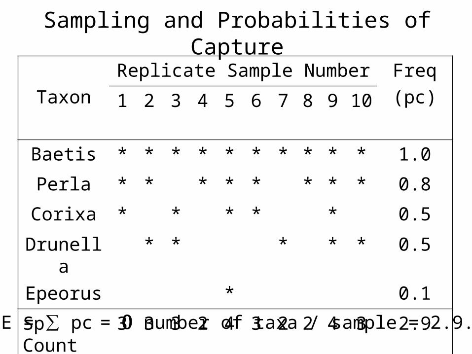
Sampling and Probabilities of Capture

Taxon

Replicate Sample Number Freq

(pc)1 2 3 4 5 6 7 8 9 10

Baetis * * * * * * * * * * 1.0

Perla * * * * * * * * 0.8

Corixa * * * * * 0.5

Drunella * * * * * 0.5

Epeorus * 0.1

Sp Count 3 3 3 2 4 3 2 2 4 3 2.9

E = ∑ pc = number of taxa / sample = 2.9.

Calculating O/E is simple…., if we can

estimate probabilities of capture.

How O/E is Calculated:

Sum of taxa pc’s estimates the number of taxa (E) that should be observed given standard sampling.

Taxon pc O

Atherix 0.92 ●

Baetis 0.86 ●

Caenis 0.70

Drunella 0.63

Epeorus 0.51 ●

Farula 0.32

Gyrinus 0.07

Hyalella 0.00

E 4.01 3

O/E = 3 / 4.01 = 0.75

O2 O3

●

●

● ●

● ●

●

3 3

Predicting E:it only hurts for a while!

• Two basic approaches:– Model many individual species (logistic

regression models) and then combine the many predictions.

– Model a few assemblage types and then ‘back out’ probabilities of capture for individual species.

– We do the latter.

Yes, explaining how E is predicted can be a little

complicated.

“In layman’s terms?

I’m afraid I don’t know any layman’s terms.”

Mc2 x R2

6.673×10-11 m3 kg-1 s-2E =

The basic approach to estimating pc’s from predictions of assemblage type was

worked out several years ago.

Moss, D., M. T. Furse, J. F. Wright, and P. D. Armitage. 1987. The prediction of the macro-invertebrate fauna of unpolluted running-water sites in Great Britain using environmental data. Freshwater Biology 17:41-52.

Empirical modeling that derives predictions of the probability of capturing a species at a new location from observations at ‘reference’ sites.

A primer is on our web page:www.cnr.usu.edu/wmc

Three Major Stepsin Estimating E

1. Classify reference sites based on their biological similarity.

2. Predict the class of a new site from environmental attributes with a discriminant functions model.

3. Weight frequencies of occurrences of taxa within classes by the site’s probabilities of class membership to estimate pc’s and then E.

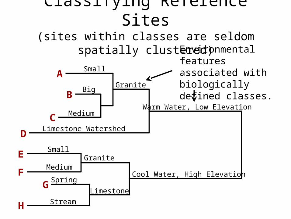
Classifying Reference Sites(sites within classes are seldom spatially clustered)

AZ_56_RefSites_logAbundance

Distance (Objective Function)

Information Remaining (%)

3.8E-02

100

2.7E+00

75

5.4E+00

50

8.1E+00

25

1.1E+01

0

R1R15R29R37R18R22R16R28R17R49R19R25R27R34R36R55R56R20R42R21R41R43R2R50R47R3R45R52R51R53R54R10R38R6R11R12R33R13R39R14R8R5R7R23R4R24R31R30R35R48R26R44R32R9R40R46

Cool Water, High Elevation

Warm Water, Low Elevation

Limestone Watershed

Granite

Granite

Limestone

Spring

Stream

Small

Medium

Small

Big

Medium

A

B

C

D

E

FG

H

Environmental features associated with biologically defined classes.

Hydropsyche 100%Caenis 95%Baetis 90%Tricorythodes 80%Drunella grandis 70%

Baetis 100%Drunella grandis 85%Arctopsyche 80%Neophylax 75%Optioservus 70%

Baetis 95%Epeorus 90%Simulium 90%Arctopsyche 75%Zapada 70%

We could use these numbers to estimate E at a new site belonging to one of these stream ‘types’, but…what if the site is ‘medium-big’, etc.?

A

B

C

Small

Big

Medium

Granite

Class A

Class B

Class C

Class D

DiscriminantAnalysis

Biologically DefinedReference Classes:

DiscriminantModel

Reference SitePredictor Variables:

Catchment AreaGeologyLatitute

LongitudeElevation

etc.

Discriminant Functions Models Classify New Sites in Terms of Their Probabilities

of Class Membership

DiscriminantModel

PredictorVariables

Values

A 0.5 0.6 0.30B 0.4 0.2 0.08C 0.1 0.0 0.00D 0.0 0.0 0.00Probability of Taxon Being in a Sampleif the Site is in Reference Condition =

0.38

Frequency

of Taxonin Class

Probability of Class

Membership

By Weighting Taxon Frequencies of Occurrence within a Class by the

Probabilities of Class Membership, We Can Estimate Individual Taxon

Probabilities of Capture

ClassContributio

nto PC

The model estimates the pc’s of every taxon (i.e., those observed in at least one reference site sample) at every assessed site, not just a few as shown here for illustration.

Also, if a taxon is predicted to have a pc of zero, it does not contribute to O!

O/E = 3 / 4.07 = 0.74

Taxon pc O

Atherix 0.70 *

Baetis 0.92 *

Caenis 0.86

Drunella 0.63

Epeorus 0.51 *

Farula 0.38

Gyrinus 0.07

Hyalella 0.00 *

E 4.07 3

Errors, inferences, and two types of assessments.

• Model error.

• Inferring site condition.

• Inferring regional conditions.

Need to Estimate Prediction Error for Site Assessments

Is a site with O/E = 0.8 impaired?

E

O

1

O/E

Statistical Issues Regarding Inferences of Impairment

(Single Samples)• Statistical Hypothesis: Is the observed

O/E value for a single sample from the same distribution of values estimated for reference sites, i.e., the site is either equivalent to reference or not.

We should ideally set a threshold value to balance Type I and II errors. Easy to set Type I error, but Type II errors are problematic. 10th and 90th percentiles of reference site values have been used.

How Good can a Model Be?• SD of O/E values calculated at reference

quality sites is a measure of overall model error.– Part sampling error– Part prediction error (random and systematic)

• A model can be no more precise than random sampling error.

• A model should be no worse than a null model – i.e., assume all sites have similar biota.

For Regional Assessments, We Want to Compare the Distribution of Observed O/E Values Among

Sites with the Expected Distribution

1

O/E

Expected if All Sites are in Reference Condition

ActualDistribution

35%

40%

25%

StreamMiles

Fair

PoorRef

Statistical Issues Regarding Inferences of Impairment

(Multiple Sites andReplicated Samples at a Site)

• Statistical Hypothesis: is the observed mean different from 1 (the reference mean)? This test allows us to ask questions regarding how impaired a site or population of sites is. Sensitivity of the test is a function of model precision and sample size. Methods for balancing Type I and II errors are well worked out. Replicate samples at a site allow estimation of confidence limits around estimates of O/E.

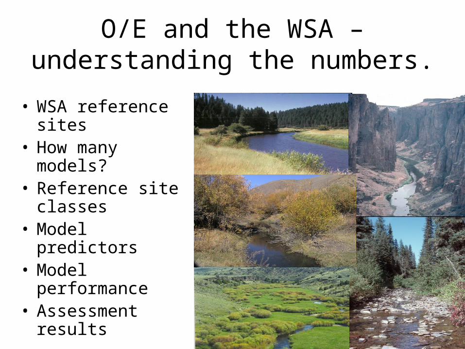
O/E and the WSA –understanding the numbers.

• WSA reference sites

• How many models?

• Reference site classes

• Model predictors• Model

performance• Assessment

results

1097 Reference Sites in ThreeSuper-Ecoregions

WEST

PLAINS EASTERNHIGHLANDS

Sample Sizes

WEST PLAINS EAST

Calibration 527 140 217

Validation 125 40 48

Great variability in geographic distribution of sites within classes.

Western Model used 30 classes of streams for

modeling

Graphic courtesy of Pete Ode.

Predictor Variables

West Plains E. Highlands

Longitude --- Longitude

Elevation Elevation ---

Day of Year Day of Year Day of Year

Basin Area Basin Area Basin Area

Stream Slope Stream Slope ---

Air Temperature Freeze-Free Days Air Temperature

Log Precipitation Log Precipitation Wet Days

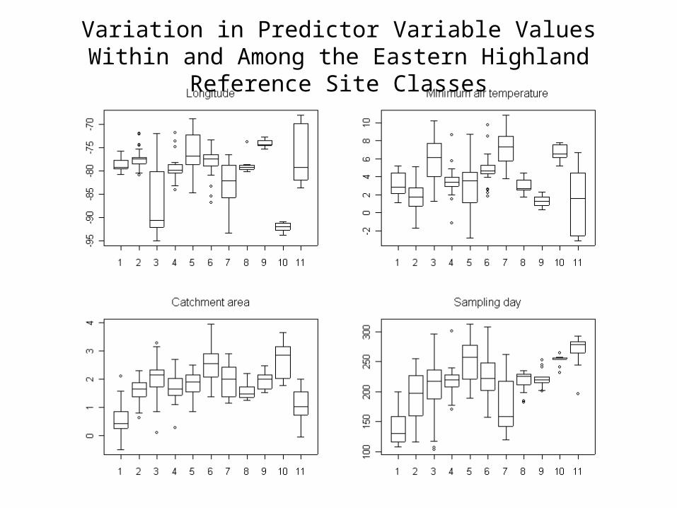
Variation in Predictor Variable Values Within and Among the Eastern Highland Reference Site Classes

Model Performance

Validation West Plains E. Highlands

Mean 0.99 0.95 0.99

SD (model) 0.20 0.24 0.18

SD (null) 0.26 0.30 0.22

Test Sites

Mean 0.84 0.86 0.81

Sites sampled for the Wadeable Streams Assessment by EPA Region.

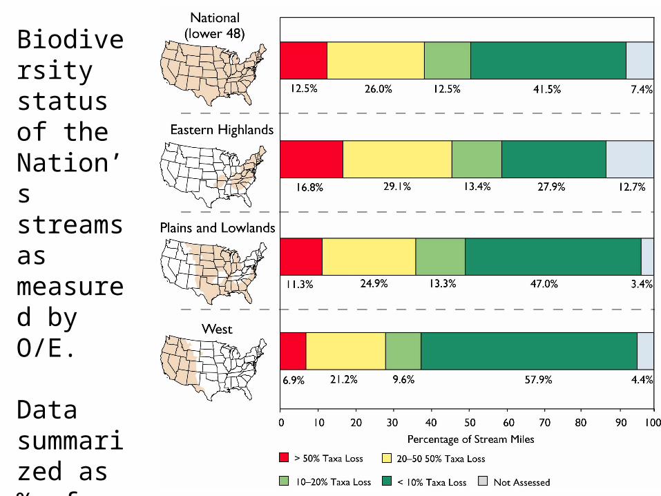
Biodiversity status of the Nation’s streams as measured by O/E.

Data summarized as % of stream miles in each of 4 O/E classes.

Concluding Remarks

• O/E has an intuitive biological meaning.

• It means the same thing everywhere.

• Its derivation and interpretation are independent of type and knowledge of stressors in the region.

• It is quantitative, but….

Our interpretations of assessments are still only as good as our understanding of aquatic ecosystems.