Developing a Numerical Model for the Design of Sheet Pile ... · Developing a Numerical Model for...

University of Southern Queensland

Faculty of Health, Engineering & Surveying

Developing a Numerical Model

for the Design of Sheet Pile Walls

A dissertation submitted by

Chane Brits

in fulfilment of the requirements of

ENG4111 and ENG4112 Research Project

towards the degree of

Bachelor of Civil Engineering (Honours)

Submitted: October 2014

ii

Abstract

This project involves the investigation, development and validation of cantilevered and

anchored sheet pile wall models. The effect of sheet pile construction penetrating a

sandy soil are investigated by analysing numerical outputs such as the wall deformation,

ground settlement and maximum bending moment. The numerical analysis is

completed using an industrially known computer software program: Fast Lagrangian

Analysis of Continua (FLAC).

The quality of the FLAC models used to obtain the numerical solutions was validated

for accuracy against available analytical solutions. The aims of this project were to gain

sufficient knowledge on sheet pile wall design methods, better known as the limit

equilibrium methods; develop an automatic Excel spreadsheet as a design tool for

solving any sheet pile wall design problem; and be able to easily validate the accuracy

of the obtained numerical solutions by comparing the numerical and analytical

solutions.

The main focus of the investigation was to develop new cantilever and anchored sheet

pile wall models for a specific geotechnical problem of a sheet pile penetrating a sandy

soil in the presence of a water table. This was done by validating the numerical models

and undertaking parametric studies varying specific parameters to investigate

thoroughly the behaviour of the sheet pile wall system.

This research concludes that the analytical methods provide a basic understanding of

the soil-wall system behaviour; however, the hypothesis on which these methods are

based makes them necessarily conservative, due to the number of assumptions required

to simplify the design procedure. Numerical modelling in FLAC produces more

accurate results and, by undertaking advanced parametric studies, indicates the actual

behaviour of the soil-wall system in the real world. The development of numerical

models, undertaking of parametric studies and validation of solutions by comparing

against analytical method solutions are areas deserving of further research, as this will

lead to more effective sheet pile wall designs in the engineering industry.

iii


Faculty of Health, Engineering and Sciences

ENG4111/ENG4112 Research Project

Limitations of Use

The Council of the University of Southern Queensland, its Faculty of Health,

Engineering & Sciences and the staff of the University of Southern Queensland, do not

accept any responsibility for the truth, accuracy or completeness of material contained

within or associated with this dissertation.

Persons using all or any part of this material do so at their own risk, and not at the risk

of the Council of the University of Southern Queensland, its Faculty of Health,

Engineering & Sciences or the staff of the University of Southern Queensland.

This dissertation reports an educational exercise and has no purpose or validity beyond

this exercise. The sole purpose of the course pair entitled ‘Research Project’ is to

contribute to the overall education within the student’s chosen degree program. This

document, the associated hardware, software, drawings and other material set out in the

associated appendices should not be used for any other purpose: if they are so used, it

is entirely at the risk of the user.

iv


Faculty of Health, Engineering and Sciences


Certification of Dissertation

I certify that the ideas, designs and experimental work, results, analysis and conclusions

set out in this dissertation are entirely of my own effort, except where otherwise

indicated and acknowledged.

I further certify that the work is original and has not been previously submitted for

assessment in any other course or institution, except where specifically stated.

Chane Brits

Student Number: 0061007950

Signature _____________________________

Date _____________________________

v

Acknowledgements

I would like to take this opportunity to give my full and sincere thanks to Dr Jim Shiau

for his continued guidance, enthusiasm and support throughout the duration of this

project. His experience and guidance on the subject has been extremely valuable and

has led to the possibility of achieving set goals to an extraordinary standard. I would

also like to thank my family for their constant support, encouragement and patience

throughout the past four years of my continuous studies. Finally, special thanks to my

fellow engineering friends Anthony Vadalma and Alejandro Aldana for all their

positive feedback and motivation during this year.

With appreciation

Chane Brits


October 2014

vi

Table of Contents

List of Figures ........................................................................................................... viii

List of Tables ................................................................................................................ x

Nomenclature .............................................................................................................. xi

Chapter 1: Introduction .............................................................................................. 1

1.1 Background .......................................................................................................... 1

1.2 Aims and Objectives ............................................................................................ 2

1.3 Overview of Chapters .......................................................................................... 3

1.4 Summary .............................................................................................................. 5

Chapter 2: Literature Review ..................................................................................... 6

2.1 Introduction .......................................................................................................... 6

2.2 Background Information ...................................................................................... 7

2.3 Classical Design Methods .................................................................................. 14

2.4 Numerical Analysis and Dissertations ............................................................... 26

2.5 Numerical Modelling Methods .......................................................................... 29

Chapter 3: Developing a Design Tool for Sheet Piles Walls .................................. 32

3.1 Introduction ........................................................................................................ 32

3.2 The Analytical Methods ..................................................................................... 33

3.3 Design Procedure for Cantilever Sheet Pile Wall .............................................. 34

3.4 Cantilever Sheet Pile Problem Description ........................................................ 38

3.5 Development of Excel Spread Sheet for the Cantilever Pile Problem ............... 39

3.6 Design Procedure for Anchor Walls .................................................................. 45

3.7 Anchored Sheet Pile Problem Description......................................................... 47

3.8 Development of Excel Spread Sheet for Anchor Wall Problem ........................ 48

3.9 Comparison between Cantilever and Anchored Pile Outputs ............................ 52

3.10 Conclusion ....................................................................................................... 53

Chapter 4: FLAC Overview ...................................................................................... 55

4.1 Introduction ........................................................................................................ 55

4.2 Major FLAC Features ........................................................................................ 56

4.3 FLAC Model Analysis ....................................................................................... 56

vii

4.4 Chapter Summary .............................................................................................. 59

Chapter 5: Numerical Analysis of Cantilever Sheet Pile Walls ............................. 60

5.1 Introduction ........................................................................................................ 60

5.2 Background Information .................................................................................... 60

5.3 Problem Description .......................................................................................... 62

5.4 Analysis using FLAC ......................................................................................... 62

Chapter 6: Numerical Analysis of Anchored Sheet Pile Walls ............................. 79

6.1 Introduction ........................................................................................................ 79

6.2 Background Information .................................................................................... 79

6.3 Problem Description .......................................................................................... 80

6.4 Analysis using FLAC ......................................................................................... 80

Chapter 7: Conclusions ............................................................................................. 92

7.1 Spread Sheet Development for Sheet Pile Wall Design .................................... 92

7.2 Cantilever Sheet Pile Wall ................................................................................. 92

7.3 Anchored Sheet Pile Wall .................................................................................. 93

7.4 Future Work ....................................................................................................... 94

7.5 Achievement of Objectives ................................................................................ 95

List of References ....................................................................................................... 97

Appendices ................................................................................................................ 101

Appendix A: Project Specification ........................................................................ 102

Appendix B: Cantilever Sheet Pile Wall-Limit State Method Calculations .......... 104

Appendix C: Anchored Sheet Pile Wall-Limit State Method Calculations ........... 111

viii

List of Figures

Figure 1-1: Retaining walls: (a) rigid wall, (b) flexible wall (Ramadan 2013) ............. 7

Figure 1-2: Cantilever Sheet Pile (Hauraki Pilling LTD) ............................................ 11

Figure 1-3: Macalloy Anchored Sheet Pile (Iceland, 2002) ........................................ 12

Figure 1-4: Failure modes for anchored sheet pile walls (Caltrans 2004) ................... 13

Figure 1-5: Failure modes for cantilevered sheet pile walls (Leila & Behzad 2011) .. 14

Figure 2-1: Full method (Padfield & Mair 1984) ........................................................ 15

Figure 2-2: Simplified method (Padfield & Mair 1984) .............................................. 16

Figure 2-3: Rectilinear Earth Pressure Distribution (Bowles 1988) ............................ 17

Figure 2-4: Case studies by Day (1999) ...................................................................... 18

Figure 2-5: Point of zero net earth pressure, presented by Day (1999) ....................... 19

Figure 2-6: Cantilever sheet pile penetrating sand (Das 1990) .................................... 20

Figure 2-7: Nature of variation of deflection and moment for anchored sheet piles:

(a) free earth support method; (b) fixed earth support method (Das

1990) ........................................................................................................... 21

Figure 2-8: Fixed Earth Support Method (Torrabadella 2013) .................................... 22

Figure 2-9: Free Earth Support Method (Torrabadella 2013) ...................................... 23

Figure 2-10: (a) Coulomb wedge analysis, (b) Rankine ‘state of stress’ analysis

(Keystone Retaining Wall Systems 2003) .................................................. 24

Figure 2-11: Blum’s equivalent beam for anchored sheet pile wall design

(Torrabadella 2013) .................................................................................... 25

Figure 3-1: Displacement of Sheet Pile Wall: (a) Cantilever (b) Anchored

(Yandzio 1998) ........................................................................................... 33

Figure 3-2: (a) Cantilever Pile Penetrating a Sandy Soil, (b) Active and Passive

Pressure Distribution (Das 1990) ................................................................ 34

Figure 3-3: Cantilever Sheet Pile Problem Definition (Das 2007) .............................. 39

Figure 3-4: Hydrostatic equilibrium of fluid motion (Szolga 2010) ............................ 43

Figure 3-5: System of forces and moments (Szolga 2010) .......................................... 44

Figure 3-6: Visual Diagrammatic Output Figures for a cantilever sheet pile .............. 45

Figure 3-7: Anchored sheet pile penetrating a sandy soil (Das 1990) ......................... 46

Figure 3-8: Anchored sheet pile problem definition (Das 2007) ................................. 48

Figure 3-9: Visual Diagrammatic Output Figures for an anchored sheet pile .............. 51

ix

Figure 5-1: (a) Cantilever Pile Penetrating a Sandy Soil, (b) Active and Passive

Pressure Distribution (Das 1990) ................................................................ 60

Figure 5-2: Cantilever Sheet Pile Penetrating Sand: (a) Net Pressure Variation

Diagram; (b) Moment Variation (Das 2007) .............................................. 61

Figure 5-3: Problem to be Investigated ........................................................................ 62

Figure 5-4: Assumed Course Mesh Grid ..................................................................... 63

Figure 5-5: Column Removed for Sheet Pile Construction ......................................... 65

Figure 5-6: Constructed Sheet Pile Wall Model .......................................................... 65

Figure 5-7: An Interface Represented by sides a, and b, connected by shear (ks)

and normal (kn) stiffness springs (FLAC 2D online manual 2009) ........... 66

Figure 5-8: FLAC Model Containing Course Mesh .................................................... 67

Figure 5-9: (a) Grid, (b) Failure Surface for initially assumed Model ........................ 68

Figure 5-10: (a) Grid, (b) Failure Surface for Fine Mesh Model with Horizontal

Increase ....................................................................................................... 69

Figure 5-11: (a) Maximum Bending Moment, (b) Maximum x-Displacement ........... 70

Figure 5-12: Plasticity Indicators for the Fine Mesh Model ........................................ 71

Figure 5-13: Visual Comparison of Maximum Bending Moment ............................... 72

Figure 6-1: Problem to be investigated ........................................................................ 80

Figure 6-2: Anchor Sheet Pile Wall Model ................................................................. 81

Figure 6-3: Node-to-node Anchors (Ramadan Amer 2013) ........................................ 82

Figure 6-4: Visual Comparison of Maximum Anchor Tie Rod Force ......................... 83

Figure 6-5: Visual Comparison of Maximum Bending Moment ................................. 84

Figure 6-6: Failure Surface Plots; for (a) Cantilever Pile, (b) Anchored Pile ............. 86

Figure 6-7: Plasticity Indicators; (a) Cantilever Model, (b) Anchor Model ................ 88

x

List of Tables

Table 3-1: Analytical Results for Cantilever Pile ........................................................ 38

Table 3-2: User Input Parameters ................................................................................ 39

Table 3-3: Designer Selection for Kp .......................................................................... 41

Table 3-4: Automatic Analysis of Analytical Equations ............................................. 41

Table 3-5: Effect of Kp Selection on Sheet Pile Wall Length ..................................... 42

Table 3-6: Important Theoretical Output Solutions ..................................................... 42

Table 3-7: Analytical Results for Anchored Pile ......................................................... 47

Table 3-8: User input data ............................................................................................ 49

Table 3-9: Automatic analysis of Analytical Equations .............................................. 49

Table 3-10: Effect of Kp Selection on Sheet Pile Wall Length ................................... 49

Table 3-11: Important Output Solutions ...................................................................... 50

Table 3-12: Comparison between Cantilever and Anchored Sheet Pile Wall ............. 52

Table 3-13: Comparison between Cantilever and Anchored Sheet Pile Wall ............. 53

Table 4-1: Grid Generation .......................................................................................... 58

Table 4-2: Soil Properties ............................................................................................ 58

Table 4-3: Pile Element Properties (ArcelorMittal 2013; Das 2007) .......................... 58

Table 4-4: Rod Anchor Properties (Ischebeck; FLAC 2D online manual 2009)......... 58

Table 4-5: Solving Analysis ......................................................................................... 58

Table 4-6: Output Variables ......................................................................................... 59

Table 5-1: Comparison of Maximum Bending Moment ............................................. 73

Table 5-2: Validation of FLAC Model ........................................................................ 73

Table 5-3: Convergence Study of Varying Mesh Fineness ......................................... 74

Table 5-4: Parametric Study of Soil Friction Angle .................................................... 75

Table 5-5: Parametric Study of Ground Water Table .................................................. 77

Table 6-1: Comparison of Maximum Bending Moment ............................................. 85

Table 6-2: Maximum Bending Moment, Maximum Wall Displacement,

Maximum Ground Settlement, and Anchor Forces with Increasing

Wall Penetration Depths ............................................................................. 89

xi

Nomenclature

The principal symbols used are presented in the following list. Locally used notation

and modifications, such as by addition of a subscript or superscript, and a symbol that

has different meanings in different contexts are defined where used.

Ka Rankine’s Active Pressure Coefficient

Kp Rankine’s Passive Pressure Coefficient

𝜙 Un-drained internal friction angle of the soil

∅′ Drained internal soil friction angle

𝜎′ Pressure at a particular depth

𝛾 ′ Effective Soil unit weight

𝛾 Soil unit weight

𝐿 Sheet Pile Length

𝛾𝑠𝑎𝑡 Saturated unit weight of the soil

𝛾𝑤 Unit weight of water

𝐷 Penetration depth of sheet pile

𝑃 Total active pressure behind sheet pile wall

𝑧 Depth below the ground surface

𝑧̅ Point of zero shear force below the ground surface

𝐴 Constant (in Chapter 3 section 3.5.3)

𝐹𝑂𝑆 Factor of safety

𝑐 ′ Drained soil cohesion

𝑀𝑚𝑎𝑥 Maximum bending moment exerted on sheet pile wall

𝐹 Anchor force

𝐷𝑡ℎ𝑒𝑜𝑟𝑒𝑡𝑖𝑐𝑎𝑙 Theoretical penetration depth of the sheet pile wall

𝐷𝑎𝑐𝑡𝑢𝑎𝑙 Actual penetration depth of the sheet pile wall

𝐴 Area (in Chapter 3 section 3.5.5)

𝑛 Number of elements

𝑃 Pressure applied over an area (in Chapter 3 section 3.5.5)

𝑑𝐴 Area differential

1

Chapter 1: Introduction

This project investigates the suitability of modelling various geotechnical sheet pile

wall problems using an explicit finite difference program, Fast Lagrangian Analysis of

Continua (FLAC). This project encompasses research into available classical theories,

current techniques of analysis and the creation of computer models. This research

discusses the geotechnical problems analysed and presents the results of an

investigation. The geotechnical problems to be investigated are:

Cantilever Sheet Pile Wall Penetrating a Sandy Soil

Anchored Sheet Pile Wall Penetrating a Sandy Soil.

1.1 Background

Geotechnical Stability

Ground stability must be assured prior to consideration of other foundation-related

items. Foundation problems involve the support of natural soil. Stability problems often

occur when building over soft, low strength soil. Problems with foundation stability can

be prevented by initial recognition of the problem and appropriate design.

The design of all structures demands ultimate and serviceability limit state requirements

to be satisfactory. Failure under ultimate limit state occurs when ‘a collapse mechanism

takes place in the ground or in some parts of the structure’ (Lancellotta 1995). The

failure mechanism can be divided into strength and stability components.

Choice of Models

The cantilever sheet pile wall was modelled as it represents further study into lateral

earth pressures acting on the sheet pile wall structure. The rotation effect of the sheet

pile wall at the bottom of the sheet pile tip results in much more complex lateral earth

pressures developing on the sheet pile wall, and hence in more complicated solutions,

only available when using numerical modelling.

2

The parametric study that will be conducted within this dissertation is a thorough study

that aims to evaluate the effect of changing certain parameters on the behaviour of the

pile-wall system. The parameters that will be investigated are:

mesh fineness

soil strength

water table effect

installation of anchor systems.

The anchored sheet pile wall model represents the possibility of decreasing the effect

of the lateral earth pressures developed on the sheet pile wall. This problem was

investigated to analyse the application of an anchor tie rod force on the behaviour of

the sheet pile wall. Knowledge of these effects will aid in future studies within the

area, as it is of upmost importance for a designer to analyse the sheet pile wall

deformation for serviceability purposes and the bending moment analyses for structural

design purposes. Due to its nature, FLAC has the potential to decrease the solution time

and increase the accuracy of the results. The outcome will be a greater understanding

of effective sheet pile wall design in the engineering industry.

Computational Analysis

Numerous methods have been developed to solve geotechnical stability problems by

hand calculations; however, modern graphical software tools have made it possible to

gain a much better understanding of the inner numerical details of soil-wall system

behaviour. Comparing the numerical solutions to the analytical solutions, it is clear that

more accurate solutions are now available by using modern computer software.

However, to obtain useful results from a computer program, it is necessary to have an

experienced user.

1.2 Aims and Objectives

The intended purpose of this dissertation is to understand the limit equilibrium methods

of analysis. The study will establish the relationship between the soil-pile system by

means of developing a numerical model and undertaking parametric studies using

FLAC. The numerical results obtained will be validated with analytical solutions to

3

evaluate the accuracy of FLAC and obtain more information and knowledge of the

system. This will lead to more effective sheet pile wall design in the engineering

industry.

The identification of appropriate milestones is an important part of reaching the major

objectives within a given timeframe. The sequence of the tasks is briefly described

below:

Research background information on the application of numerical analysis for

geotechnical design.

Create a spread sheet in Excel that will automatically solve for any sheet pile

wall design. Aim for this spread sheet to be useable in the engineering industry.

Gain sufficient knowledge of the software program FLAC, to enable the writing

of a script code using FLAC’s inner built-in coding language, FISH. This will

make it possible to create an anchored sheet pile wall model in FLAC.

Undertake parametric studies in FLAC by means of varying specific parameters

to determine the effect of the net pressure, shear forces and bending moments

applied on the sheet pile wall.

Compare the results obtained from the analytical methods with the results

gathered from the numerical applied analysis to verify the numerical methods.

1.3 Overview of Chapters

This chapter overview gives a brief introduction to the task, methodology and the

computer program to be utilised. Following this, each problem is investigated

separately, including validation and advanced parametric studies to analyse the

behaviour of the sheet pile wall. The dissertation concludes with an overall summary

and an outline of possible future work.

Chapter 1: Introduction

This chapter provides an outline of the study, as well as an introduction to the problem

and the essential background information. The chapter also discusses the project

objectives and main aim for the dissertation.

4

Chapter 2: Literature Review

This chapter presents a literature review of all the past studies for the design of

cantilevered and anchored sheet pile wall problems. Included within the literature

review are current available analytical methods for the design of sheet pile walls, as

well as findings and results from past dissertational FLAC modelling of sheet pile walls.

The previous work is used to determine why additional research is necessary and the

scope of the research required.

Chapter 3: Developing Tools for Sheet Pile Wall Design

In this chapter, the methodology for designing sheet pile walls is introduced. Indicated

in this chapter is the development of design tools such as an automated spread sheet

that can automatically solve any sheet pile wall problem, solving tedious analytical

equations within seconds by simply inputting known data specified by the user. The

generated design tools are then used as part of the validation process of the numerical

models.

Chapter 4: FLAC Overview

This chapter presents a short introduction to the FLAC software package, as well as an

overview of the FLAC script that was generated to model the geotechnical problem.

The methodology used for specifying the inputs required the development of a

numerical model that leads to the validation of the models and specific outputs obtained

from FLAC.

Chapter 5: FLAC Analysis of Cantilever Sheet Pile Wall

Presented in this chapter is the creation of a numerical cantilever sheet pile wall model

for a specific sheet pile wall problem. This chapter specifies the process required for

validating numerical model graphical outputs and obtaining qualitative results. Within

5

this chapter, advanced modelling by means of undertaking a parametric study has been

presented to illustrate the overall soil-pile system behaviour.

Chapter 6: FLAC Analysis of Anchored Sheet Pile Wall

Presented in this chapter is the creation of a cantilever sheet pile wall model for the

specific geotechnical sheet pile wall problem. This chapter presents the validation of

the numerical model, as well as advanced modelling of anchorage sheet pile wall

systems, to investigate specific parameters that have a ‘real life’ effect in the

engineering industry.

Chapter 7: Conclusions and Future Work Recommendations

This chapter presents the overall findings presented within Chapters 3–6. This chapter

presents a summary of the conclusion of the dissertation. Recommendations for further

work are discussed to ensure that this work is clearly defined.

1.4 Summary

The basic understanding of the studies to be undertaken was presented in this chapter

to give an overview of the chapters that follow. From this chapter, it is evident that

many aspects need to be considered throughout the duration of this project. Sheet pile

wall problems consist of a very complex soil-wall system and it is therefore important

that all aspects of the problem are covered. The following chapter presents a detailed

literature review of past studies relating to the investigations that have been conducted

within this dissertation.

6

Chapter 2: Literature Review

2.1 Introduction

There are several sheet pile walls design methods dating back to the first half of the

twentieth century. These original proposals have been continuously and may currently

be being reviewed (Torrabadella 2013). Analytical methods include ‘limit stage design

methods’ or ‘classical methods’ (King 1995). For establishing equilibrium of the

horizontal forces and moments developed along the wall and to define the failure state

point along the sheet pile and the embedment depth below the dredge line for either

cantilever or anchored sheet pile walls by means of undertaking geotechnical design,

calculations are required regardless of the method adopted.

The estimation of the limit equilibrium method depends on the limiting earth pressure

coefficients from plastic theories. The earth pressure forces on the wall are also

calculated with these plastic theory values. During the limit equilibrium condition, the

equilibrium equations are used to deduce the driven depth of the sheet pile wall. A

factor of safety is applied by an increase in sheet pile depth to limit the movement of

the wall and take into account any possible errors in the soil parameters and analysis.

The second approach, the finite element technique, first proposed by Morgenstern and

Eisentein (1970), often makes use of the finite element technique to solve the stiffness

equations. Satisfactory knowledge of the stress-strain behaviours of the soil and its

parameters is necessary, as this indicates the behaviour of the soil-structure system.

The limit equilibrium methods are based on the prediction of maximum excavation

height, for which static equilibrium will be maintained. This is known as the classical

design methods. The accuracy of the earth pressure evaluation acting on either side of

the wall in the condition of limit equilibrium is very important. The generated earth

pressure exerted on the sheet pile wall is due to the actual distribution and magnitude

of these pressures and is dependent on the complex soil-wall interaction.

7

Equilibrium for an anchored sheet pile wall with only a single row of anchors can be

achieved without taking into consideration the passive reaction at the bottom of the

back of the sheet pile wall. However, the design method used can change depending on

whether this reaction force is considered. When comparing the cantilevered and

anchored sheet pile walls, the main advantage found from the anchored sheet pile wall

is its ability to reduce the embedment depth of the sheet pile, thus increasing the

excavation depth, which has a profitable effect on the structure (Das 1990). It is

important to note that due to the anchor provided, the excavation depth can be

increased, but the structure behaves like a cantilever sheet pile only until the anchor is

placed (Torrabadella 2013).

2.2 Background Information

Retaining walls are used to hold back soil and maintain a difference in the elevation of

the ground surface. Retaining walls can be classified into two categories of structure:

rigid or flexible. A wall is considered rigid if it moves as a unit and does not produce

wall deformation. Most gravity walls such as masonry walls, simple concrete walls or

reinforced concrete walls can be considered rigid. Flexible walls, by contrast, undergo

wall deformations. The most common flexible sheet piles are steel sheet piles, due to

their tolerance of large deformation occurrences. Typical examples of these two types

of retaining wall are indicated in Figure 1-1.

Figure 1-1: Retaining walls: (a) rigid wall, (b) flexible wall (Ramadan 2013)

8

Sheet pile walls consist of driven, vibrated or pushed interlocking pile segments

embedded into soils to resist horizontal pressures. The sheet pile walls are constructed

by driving the sheet piles into a slope or excavation. They are considered most cost-

effective where retention of higher earth pressures of soft soils is required. Sheet piles

have a significant advantage in that they can be driven to depths below the excavation

bottom and so provide a control to heaving in soft clays or piping in saturated sand.

Sheet piles can function as temporary or permanent structures and are most often used

in excavation projects. Temporary sheet piling structures are used to control or exclude

earth or water and allow the continuation of permanent work. Permanent sheet piling is

commonly used as a retaining structure, and at times as part of the structure of

underground buildings (Paikowsky & Tan 2005).

When sheet pile walls are constructed, important design parameters are introduced that

are often difficult to evaluate, making the design process complex and protracted. The

generation of an automatic design tool in Excel to solve any sheet pile wall problem

would help to overcome these design difficulties and time issues; not only by leading

to easier evaluation, but also by making it possible to obtain results quickly for

undertaking the validation process.

Numerical modelling has evolved over the years. Research has found that these

numerical methods for the design of sheet pile walls are very useful and can be used to

obtain information that is unavailable when using analytical methods for the design of

sheet pile walls (Smith 2006; Bilgin 2010); that is, the wall deformation, ground

settlement and possible surface failures. This research uses FLAC to develop its

numerical model. FLAC is a popular industrially known design tool, used to solve

geotechnical problems.

Sheet Pile Wall Materials

Sheet pile walls are made of different kinds of materials such as wood, concrete, steel

or aluminium. The material selection depends on a number of factors, including

strength and environmental requirements. The designer must consider the possibility of

material deterioration and its effect on the structural integrity of the system. Most

9

enduring structures are constructed of steel or concrete. Concrete is capable of

providing a long service life under normal conditions, but has relatively high initial

costs when compared to steel sheet piling. Concrete piling is also more difficult to

install than steel piling. Long-term field observations indicate that steel sheet piling

provides a long service life when properly designed (Ramadan Amer 2013).

The steel sheet pile alternative is the most popular due to its strength, ease of handling

and construction. Steel sheet piles are available in various cross-section shapes. They

can have problems with corrosion that can be prevented by coating. They can be used

above or below water provided the required protection is applied (Bowles 1988).

Their advantages are:

resistant to high driving stresses

relatively lightweight

reusable

long service life

easy to increase length by welding

joints are less likely to deform

can produce a watertight wall.

Other materials such as vinyl, polyvinyl chloride and fiberglass are also available.

These pilings have very low structural capacities and function in tieback situations.

When compared to other materials, only short lengths of pile are available. The designer

for each sheet pile application when using one of the above-mentioned materials must

carefully evaluate the properties of the specific material obtained from the manufacturer

(Paikowsky & Tan 2005).

Steel is the most common material used for sheet pile walls and is thus considered as

the main sheet pile wall material in this dissertation.

10

Construction of Sheet Pile Walls

The construction of sheet pile walls may involve either excavation of soils in front or

backfilling of soils behind the wall; that is, fill construction or cut construction. Fill

wall construction refers to a wall system in which the wall is constructed from the base

of the wall up to the top: also called ‘bottom-up’ construction. Cut wall construction

refers to a wall system in which the wall is constructed from the top of the wall down

to the base, concurrent with excavation operations: known as ‘top down’ construction

(Zhou 2006). These construction procedures generate different loading conditions in

the soil and thus different wall behaviour should be expected (Das 1990).

Sheet pile walls are widely used in excavation support systems, cofferdams and cut-off

walls under dams, slope stabilisation, waterfront structures and floodwalls. Sheet pile

walls used to provide lateral earth support could be either cantilever or anchored

depending on the wall height. Recently, land owners have been seeking to maximise

the usage of their land by designing basements up to their land boundaries, with little

regard for the subsoil and site condition restraints. The result is that various deep

excavations are carried out in close proximity to existing buildings and infrastructures,

increasing the importance in design of considering the safety of neighbouring structures

(Kasim 2011).

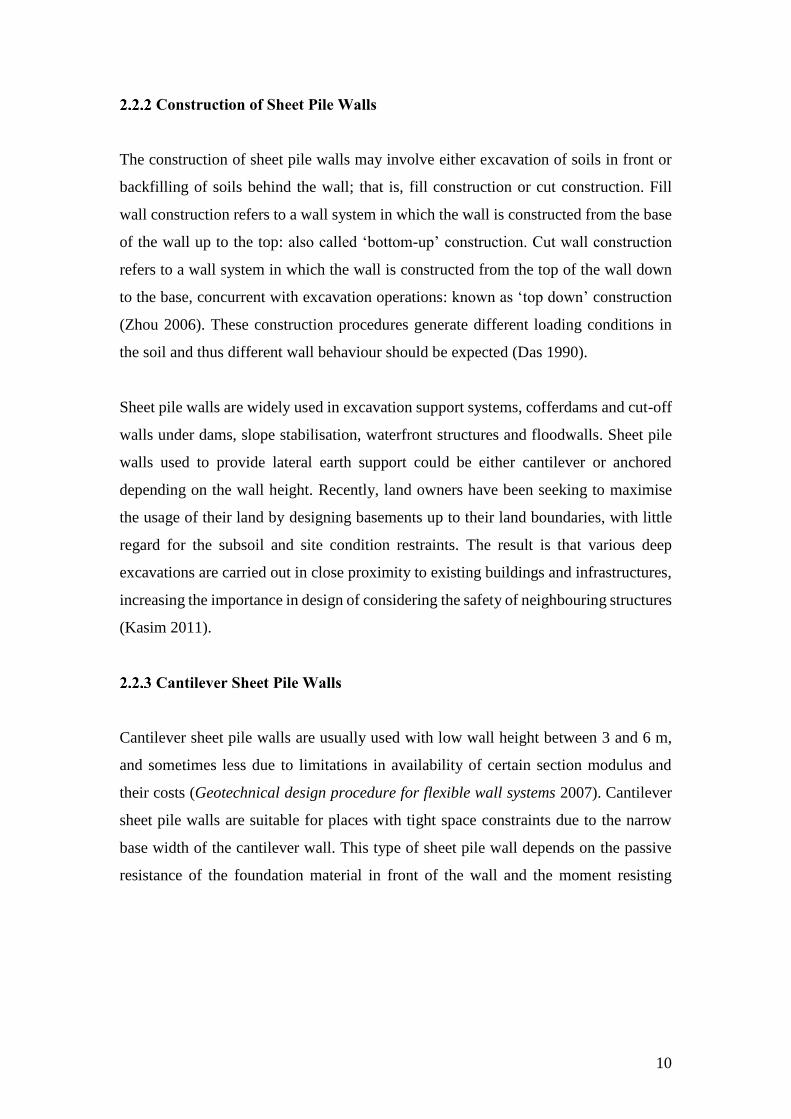
Cantilever Sheet Pile Walls

Cantilever sheet pile walls are usually used with low wall height between 3 and 6 m,

and sometimes less due to limitations in availability of certain section modulus and

their costs (Geotechnical design procedure for flexible wall systems 2007). Cantilever

sheet pile walls are suitable for places with tight space constraints due to the narrow

base width of the cantilever wall. This type of sheet pile wall depends on the passive

resistance of the foundation material in front of the wall and the moment resisting

11

capacity of the piles for stability (Figure 1-2). Therefore, it should not be used where

the foundation material may be removed during wall service life (Caltrans 2004).

Figure 1-2: Cantilever Sheet Pile (Hauraki Pilling LTD)

Anchored Sheet Pile Walls

Anchored sheet pile walls are required when the wall height exceeds 6 m or when the

lateral wall deflection is limited for design consideration (Leila & Behzad 2011).

Anchoring the sheet pile wall requires less penetration depth and also less moment to

the sheet pile because it will drive additional support by the passive pressure on the

front of the wall and the anchor tie rod. Anchored sheet pile walls are typically

constructed in cut situations, and may be used for fill situations with special design

considerations to protect the anchor from construction damage from fill placement or

fill settlement (Geotechnical design procedure for flexible wall systems 2007).

Several types of anchors can be used with sheet pile walls, such as dead-man and

grouted tiebacks. Temporary support can also be provided for the walls by making use

of struts, braces and rakers (Geotechnical design procedure for flexible wall systems

2007). The selection of the most suitable type of anchor generally depends on the soil

type, presence of groundwater and cost considerations (Elias & Juran 1991). For

situations in which one or more levels of anchor are required, it is most suitable to make

use of grouted tiebacks, whereas the suitability of tie dead-man anchors is typically

limited to situations requiring a single level of anchor (Caltrans 2004).

12

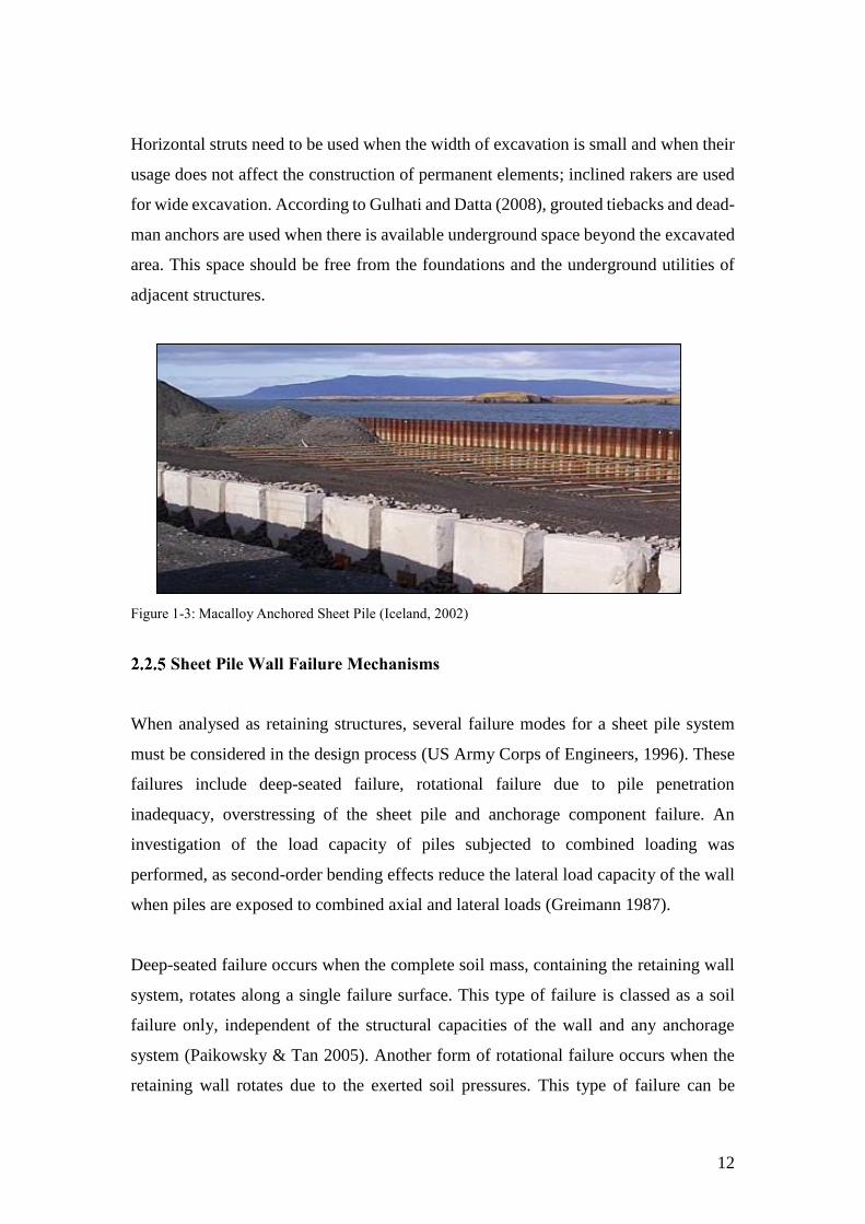
Horizontal struts need to be used when the width of excavation is small and when their

usage does not affect the construction of permanent elements; inclined rakers are used

for wide excavation. According to Gulhati and Datta (2008), grouted tiebacks and dead-

man anchors are used when there is available underground space beyond the excavated

area. This space should be free from the foundations and the underground utilities of

adjacent structures.

Figure 1-3: Macalloy Anchored Sheet Pile (Iceland, 2002)

Sheet Pile Wall Failure Mechanisms

When analysed as retaining structures, several failure modes for a sheet pile system

must be considered in the design process (US Army Corps of Engineers, 1996). These

failures include deep-seated failure, rotational failure due to pile penetration

inadequacy, overstressing of the sheet pile and anchorage component failure. An

investigation of the load capacity of piles subjected to combined loading was

performed, as second-order bending effects reduce the lateral load capacity of the wall

when piles are exposed to combined axial and lateral loads (Greimann 1987).

Deep-seated failure occurs when the complete soil mass, containing the retaining wall

system, rotates along a single failure surface. This type of failure is classed as a soil

failure only, independent of the structural capacities of the wall and any anchorage

system (Paikowsky & Tan 2005). Another form of rotational failure occurs when the

retaining wall rotates due to the exerted soil pressures. This type of failure can be

13

prevented by adequate wall penetration into the soil or by implementing an anchorage

system.

The other failures that may occur in retaining wall systems are sheet pile overstressing,

passive anchorage failure, tie rod failure and wale system failure (Figure 2-4). In the

case of pile overstressing due to both lateral and axial loads, a plastic hinge leading to

failure will develop.

When the anchor moves laterally within the soil due to the force exerted on it, a passive

anchorage failure will occur. The tie rod may fail if the required tensile capacity is not

adequate, and the wale system may undergo a bearing failure if the loads are not evenly

distributed (Evans 2010).

Figure 1-4: Failure modes for anchored sheet pile walls (Caltrans 2004)

14

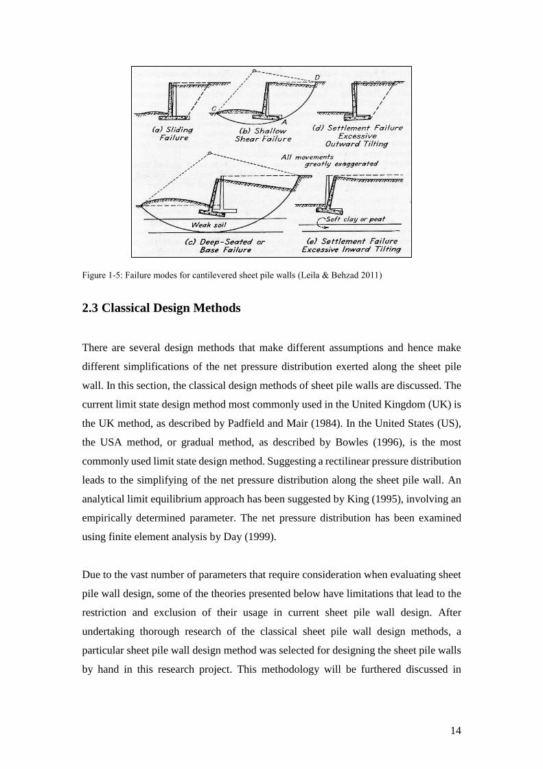
Figure 1-5: Failure modes for cantilevered sheet pile walls (Leila & Behzad 2011)

2.3 Classical Design Methods

There are several design methods that make different assumptions and hence make

different simplifications of the net pressure distribution exerted along the sheet pile

wall. In this section, the classical design methods of sheet pile walls are discussed. The

current limit state design method most commonly used in the United Kingdom (UK) is

the UK method, as described by Padfield and Mair (1984). In the United States (US),

the USA method, or gradual method, as described by Bowles (1996), is the most

commonly used limit state design method. Suggesting a rectilinear pressure distribution

leads to the simplifying of the net pressure distribution along the sheet pile wall. An

analytical limit equilibrium approach has been suggested by King (1995), involving an

empirically determined parameter. The net pressure distribution has been examined

using finite element analysis by Day (1999).

Due to the vast number of parameters that require consideration when evaluating sheet

pile wall design, some of the theories presented below have limitations that lead to the

restriction and exclusion of their usage in current sheet pile wall design. After

undertaking thorough research of the classical sheet pile wall design methods, a

particular sheet pile wall design method was selected for designing the sheet pile walls

by hand in this research project. This methodology will be furthered discussed in

15

Chapter 3. In addition, in Section 2.4, discussion is presented of some dissertations on

numerical sheet pile wall design (Smith 2006; Ramadan 2013; Torrabadella 2013).

Padfield and Mair (1984) Design of Retaining Walls in Stiff Clays

The full UK method gets its name in contrast to the simplified method, described below.

In the full method, the active limit state is assumed to be reached in the back of the wall

above the rotation point, and the passive limit state is assumed to be reached in front of

the wall between the dredge line and the rotation point. Supposedly, an overturn in the

normal pressure direction is to be produced at the rotation point, below which the full

passive pressure is moved behind the wall and the active to the front. This causes a

sudden jump in the earth pressure, which is needed to prescribe moment equilibrium.

Figure 2-1: Full method (Padfield & Mair 1984)

16

Due to the complexity of the full method, a simplification was recommended by

Padfield and Mair (1984). As shown in Figure 2-2, the earth pressure below the rotation

point can be replaced by an equivalent concentrated force acting on point O, represented

as the resultant force. The value for the depth d has been found to be considerably lower

than compared to the value calculated by the full method. Thus, the simplified method

is slightly more conservative than the full method, although it leads to appreciably

similar results.

Figure 2-2: Simplified method (Padfield & Mair 1984)

17

Bowles (1988) Foundation Analysis and Design

A rectilinear net earth pressure distribution was proposed by Bowles (1988) in which

the active earth pressure in the back of the wall above the dredge line and passive earth

pressure in front of the wall immediately below the dredge line were fully mobilised

even before failure. The design depth of penetration was calculated by finding the z in

Figure 2-3, corresponding to the maximum net earth pressure in front of the wall,

satisfying both equilibrium of horizontal forces and moments about the bottom of the

wall.

Figure 2-3: Rectilinear Earth Pressure Distribution (Bowles 1988)

A slightly different approach was later reviewed that does not involve the hypothesis

of a sudden change in the earth pressure distribution. The assumption made in this

method is to consider the transition zone at which the net earth pressure gradually

changes its direction from the front to the back of the wall. The rotation point is where

the transition occurs and is also assumed to be linear. This gradual method is also

known as the general rectilinear net pressure method or the USA method, as presented

by Skrabl (2006) and Day (1999).

18

Day (1999) Net Pressure Analysis of Cantilever Sheet Pile Walls

Day (1999) presented a finite element study in which the net earth pressure over the

sheet pile wall was examined. In the finite element study conducted by Day (1999), five

case studies were considered, consisting of wall heights of 10 m and soil friction angles

ranging between 20 and 50 degrees with variable excavation depths. The results

indicated that a dependent relationship exists between the point of zero net pressure and

the ratio between the active and passive pressure distributions (Figure 2-4).

Figure 2-4: Case studies by Day (1999)

19

Day proposed an equation to define the point of zero pressure (Figure 2-5). This

equation proposed a linear relation between the position of the point of zero pressure

and the ratio of Kp to Ka. The proposal by King (1995) that 𝜀′ = 0.35 is generally

conservative.

Figure 2-5: Point of zero net earth pressure, presented by Day (1999)

The rectilinear net pressure distribution and pressure coefficients predicted by Caquote

and Kerisel are more accurate than the existing design methods commonly used in the

UK and US. According to Day (1999), the predictions for both the critical retained

height and the bending moment distribution using the empirical equations agree

excellently when compared to the finite element numerical results for cantilever sheet

pile walls. The finite element results are in fact in better agreement with Caquote and

Kerisel’s results than the existing design analytical methods.

Das (1990) Principles of Foundation Engineering

Cantilever sheet pile walls are usually recommended for retaining walls of moderate

height (6 m or less, measured above the dredge line). According to Das (1990), such

piles act as wide cantilever beams. The basic principles proposed by Das (1990) are

explained in the figure on the following page, which indicates the nature of lateral

yielding of a cantilever wall penetrating a sand layer below the dredge line.

20

The wall rotates about a point O (Figure 2-6 [a]). The hydrostatic pressures on either

side of the sheet pile wall are assumed to cancel each other out; thus, only considering

the effective lateral soil pressure below the dredge line to act on the sheet pile was

assumed. In zone A, the lateral pressure is just the active pressure from the land side;

however, in zone B, there will be active pressure from the land side as well as passive

pressure from the water side due to the yielding occurrence of the wall. The condition

in zone C is reversed, which is below the point O. The actual net pressure distribution

on the wall is shown in Figure 2-6 (b), and a simplified version is illustrated in Figure

2-6 (c).

Figure 2-6: Cantilever sheet pile penetrating sand (Das 1990)

When the height of the backfill material behind a cantilever sheet pile wall exceeds 6

m, anchor sheet pile wall becomes more economical. According to Das (1990), this

type of construction is referred to as an anchored sheet pile wall or an anchored

bulkhead. Das specifies that the presence of anchors decreases the penetration depth of

the sheet pile and reduces the cross-sectional area and weight of the sheet piles.

However, Das (1990) suggests that the anchors be designed with care.

21

The two basic methods of designing anchored sheet pile walls are (a) the free earth

support method and (b) the fixed earth support method. According to Das (1990), the

free earth support method involves a minimum penetration depth to be obtained and the

absence of a pivot point for the static system (Figure 2-7).

Figure 2-7: Nature of variation of deflection and moment for anchored sheet piles: (a) free earth support

method; (b) fixed earth support method (Das 1990)

22

Fixed Earth Support Method for Anchored Piles

In the fixed earth support method, the sheet pile is embedded deeply in comparison with

the height above the dredge level in such a way as to ensure that the passive pressure in

front of the wall is no longer fully mobilised. An overturn in the normal earth pressure

is achieved by means of the increasing embedment depth. The earth pressure

distribution results is similar to that achieved for the cantilever sheet pile wall (Figure

2-8). The wall behaves as if partially built-in and being subjected to bending moments

(United States Steel 1975).

Figure 2-8: Fixed Earth Support Method (Torrabadella 2013)

Free Earth Support Method for Anchored Pile

The movement on the embedded zone of the wall has been assumed sufficient to

mobilise both the active and passive pressures behind and in front of the wall,

respectively. Thus, the method is based on the assumption to satisfy stability of the

sheet pile against lateral displacement by means of driving the sheet pile only deep

23

enough to withstand such pressures (Shanmugam 2004; Das 1990). The entire depth of

embedment mobilises the shear strength of the soil (Figure 2-9).

Proceeding then by means of summing the moments with respect to the point of applied

anchor force and equating the expression to zero, the minimum embedment depth is

calculated to provide equilibrium.

Figure 2-9: Free Earth Support Method (Torrabadella 2013)

The theory and assumptions made by Das (1990) for the development of the lateral

earth pressures exerted on the sheet pile wall are based on Rankine theory. There are

two commonly accepted methods for calculating simple earth pressure (Keystone

Retaining Wall Systems 2003): Coulomb and Rankine theory. The Coulomb theory was

developed in 1776, while the Rankine theory was developed in 1857. These theories,

which remain the basis for present-day earth pressures calculation, are based on the

fundamental assumptions that the retained soil is:

cohesionless

homogenous

isotropic

semi-finite

well drained.

24

The active earth pressure calculation requires that the wall structure rotates or yields

sufficiently to engage the entire shear strength of the soils involved to create the active

earth pressure state. The amount of movement highly depends on the soil that is

involved.

Both theories use identical parameters; however, Coulomb wedge theory calculates less

earth pressure than Rankine theory (Figure 2-10). This indicates that the results

obtained from the Rankine theory will be more conservative. Das (1990) made use of

these conservative methods for the design of sheet pile walls.

Figure 2-10: (a) Coulomb wedge analysis, (b) Rankine ‘state of stress’ analysis (Keystone Retaining Wall

Systems 2003)

Blum’s (1931) Equivalent Beam Method Theory for Anchored Piles

Blum’s equivalent beam method theory is used to find the embedment depth, by

analysing the sheet pile as a beam structure. The beam is divided into two sections: an

upper beam and a lower beam. In the upper beam, the net pressure acts against the back

of the wall; in the lower part of the beam, the net pressure action is placed in front of

the wall.

25

The moments are taken around the point in line with the anchor force for the upper part

of the beam to find the force Rb; in the lower beam, moments are taken at the bottom to

find the embedment depth (Figure 2-11). The embedment depth must be increased to

ensure that the reaction Rc can be engaged (Azizi 2000; Bowles 1996; Tsinker 1997).

Figure 2-11: Blum’s equivalent beam for anchored sheet pile wall design (Torrabadella 2013)

Conclusion of Classical Method Design

The comparison of the method proposed by Das (1990) with other currently used

methods has shown that the results obtained compare well with the numerical finite

element results provided by Day (1999) and Smith (2006). Using the analytical method

proposed by Das (1990) can thus be considered successful for validating numerical

solutions for cantilever sheet pile wall models against the analytical solutions. This

method is used in the relevant chapters that follow.

26

2.4 Numerical Analysis and Dissertations

Smith (2006), Development of Numerical Models for Geotechnical Design

Smith (2006) investigated a cantilever sheet pile wall penetrating sand in the absence

of a water table using the finite difference method software, FLAC. The numerical

results obtained from the numerical model developed in FLAC were then compared to

the analytical solutions and the advantages and disadvantages were discussed. The

depth of embedment was then varied to identify the effect exerted on the sheet pile wall

by analysing the bending moment, wall deflection and ground settlement. Smith’s

(2006) investigation demonstrated that FLAC produced similar results to the limit

equilibrium methods. The outputs obtained were also found to be more accurate when

compared to the limit equilibrium method solutions. Smith (2006) suggested the

possible future work of undertaking numerical parametric studies using the cantilevered

sheet pile wall model to develop an anchored sheet pile wall model. Performing

parametric studies was also deemed valuable for the advanced analysis of the behaviour

of the sheet pile walls.

Bilgin (2010), Numerical Studies of Anchored Sheet Pile Wall Behaviour

Constructed in Cut and Fill Conditions

Construction of sheet pile walls involves either excavation in front or backfilling of soil

behind the wall. Different loading conditions in the soil are generated due to the

construction procedures, generating different wall behaviours. The conventional

methods used in the design of anchored sheet pile walls, which are based on the limit

equilibrium approach, do not consider the method of construction. However, continuum

mechanics numerical methods, such as the finite element method, make it possible to

incorporate the construction method into the analysis and design of sheet pile walls.

This allows for the analysis of the soil-wall system, to obtain more viable and accurate

solutions. Bilgin (2010) investigated the effect of wall construction by varying soil

conditions and wall heights using finite element modelling. The construction method’s

influence on the wall behaviour in terms of wall deformation, wall bending moments

and anchor forces were investigated, with Bilgin (2010) concluding that construction

using backfilling produces significantly higher bending moments and wall

27

deformations. These findings indicate that there are limitations to be considered when

using the limit equilibrium methods, and that more information can be obtained by

undertaking numerical analysis (Bilgin 2010).

Bilgin (2012), Lateral Earth Pressure Coefficient for Anchored Piles

According to Bilgin (2012), the design of anchored sheet pile walls established by the

conventional methods is based on the lateral force and moment equilibrium of active

and passive earth pressure and anchor forces. Bilgin (2012) carried out a parametric

study using both conventional and numerical methods to investigate the behaviour of a

single-level anchored sheet pile wall. The effect on the wall lateral earth pressures, wall

moments and anchor forces was investigated. The results obtained indicated that the

free earth support method over-estimates the bending moments, whereas the anchor

forces were underestimated. Interestingly, new lateral earth pressure coefficients that

took the stress concentration around the anchor level into account were used in the

design, which led to more realistic earth pressure distributions acting on the wall, as

well as more accurate anchor sheet pile wall designs.

Ramadan (2013), Effect of Wall Penetration Depth on the Behaviour of

Sheet Pile Walls

The purpose of this dissertation was to analyse the wall penetration depth on sheet pile

wall behaviour. According to Ramadan (2013), important serviceability considerations

are not considered when using the limit equilibrium methods. This is because

information about the wall deformation cannot be obtained by these analytical methods.

Ramadan (2013) investigated wall behaviour by varying the soil conditions for both the

cantilever and anchored sheet pile walls. Finite element analysis was then used to

perform numerical modelling to analyse the behaviour of the walls and the structural

response. It was found that wall deformations reduce with increasing wall penetration

depth for both wall types and the bending moments significantly reduced with

increasing wall penetration depth.

28

Torrabadella (2013), Numerical Analysis of Cantilever and Anchored Sheet

Pile Walls at Failure and Comparison with Classical Methods

Torrabadella (2013) analysed the influence of the initial stress state condition on the

horizontal displacement of sheet pile walls. It was found that for K0 values between 0.7

and 0.9, minimum movement was registered at the top of the pile; however, the initial

stress state also depended on the soil friction angle. Depending on the initial stress state,

the wall movement was found potentially to change up to 40%. The influence of the

construction procedure also had a critical effect on the wall movement. For anchored

piles, it was found that when the anchors were pre-stressed, movement was absorbed,

limiting wall strains. In contrast to cantilever sheet pile walls, the maximum horizontal

displacement was found at a particular depth and not at the ground surface. A direct

effect between the anchor force and horizontal wall displacement was found.

Torrabadella (2013) also found that the limit equilibrium methods corresponded well

with the numerical methods for both cantilever and anchored sheet pile walls.

Zhai (2009), Comparison Study for the Seismic Evaluation of Anchored

Sheet Pile Walls

In Zhai’s (2009) study, the seismic stability and deformation of the channel bank and

the anchored sheet pile wall subjected to a design earthquake load were investigated by

analysing the results obtained from three different engineering approaches: the limit

equilibrium methods, the p-y method and the time history soil structure (SSI) analysis

method. It was found that the values obtained using FLAC (as the SSI method) for the

maximum bending moment and anchor rod force were about 55% and 73% of the

values obtained from the earth pressure method. For seismic stability, the system was

found to be unstable when using the earth pressure method, but stable when using the

SSI method (Zhai 2009).

29

2.5 Numerical Modelling Methods

Most engineering problems involve complex physical phenomena (Chaskalovic 2008).

To gain a good understanding of these phenomena, engineers normally make simplified

assumptions that allow the formulation of mathematical models (Pastor & Tamagnini

2004; Wood 2003).

Numerical analysis has evolved over the past few decades (Chaskalovic 2008),

followed by prompt advances and improvements in modern computer technology (Rao

2005; Zienkiewicz, Taylor & Zhu 2013; Desai and Christian 1977). This will lead to

the ability to undertake procedures, algorithms and other numerical techniques capable

of solving ever more complex engineering problems. However, it is important for an

engineer to know that with these numerical methods certain limitations, uncertainties

and approximations need to be considered (Wood 2003). This leads to more

computationally based studies being carried out in the geotechnical engineering

industry. It is important that the results obtained from the numerical methods are

validated against conventional or analytical methods (Pande & Pietruszczak 2004).

Industrially Commonly Known Numerical Analysis

The most common numerical techniques used currently in the geotechnical engineering

industry are the finite difference method (FLAC) and the finite element method

(PLAXIS). Finite difference methods were almost exclusively used in obtaining

numerical solutions for geotechnical problems prior to the establishment of the finite

element methods. The finite element method is considered one of the most important

developments in civil engineering of the twentieth century (Papadrakakis 2001).

Background of FLAC Software

FLAC is a two-dimensional (2D) explicit finite difference software program, developed

by Dr Peter Cundall in 1986 (FLAC 2D online manual 2009). This software makes it

possible to visualise the behaviour of the structure in the soil, rock or any other material

that may undergo plastic flow. A grid of the materials can be formed that represents

30

elements or zones that can be adjusted by the user. This explicit, Lagrangian calculation

scheme and the mix-discretisation zoning technique used in FLAC ensure the highly

accurate modelling of flow and plastic collapse. Large 2D calculations can be made

without the need for massive memory requirements due to no matrixes being formed.

FLAC was originally developed for geotechnical and mining engineers. This software

offers a wide range of capabilities, including for solving complex problems in

mechanics. The FLAC software has special built-in functions that make it unique. The

application range of FLAC is extensive because it is equipped with 11 built-in

constitutive models, five optional facilities and several kinds of structure elements as

well as a built-in coding language, FISH (Shen 2012).

Other element structures present in FLAC include beam, anchor, pile and shell

structures. These elements are used to create more realistic models of geotechnical

engineering problems in the software. It will be useful to design an anchored sheet pile

wall model in FLAC. The build-in coding language (FISH) can also be used to define

new functions and variables to meet user demands.

FLAC Software Advantages and Disadvantages

The FLAC software, used here to develop a numerical model for the design of sheet

pile walls, has several advantages over other methods (FLAC 2D online manual 2009):

The mix-discretisation zoning method is more accurate than the reduced

integration method generally used to simulate the plastic flow of materials.

The explicit methods used decrease the time needed to solve non-linear

equations.

The full dynamic equation of motion is used, making the software more suitable

to simulate problems involving vibration, failure and large deformations.

The element numbering is done in row and column formatting.

There are also some disadvantages when using FLAC that need to be considered (FLAC

2D online manual 2009):

More time is needed to reach convergence for a linear problem than when using

the finite element methods.

31

FLAC depends on the ratio of maximum and minimum natural periods of the

system for the convergence velocity.

Thorough research has shown that FLAC is an excellent software choice for modelling

any geotechnical engineering model. Therefore, FLAC is used to undertake the

numerical modelling in this dissertation.

32

Chapter 3: Developing a Design Tool for Sheet Piles Walls

3.1 Introduction

Nowadays, the engineering profession is discovering and using the computational

powers of computer spread sheets in practice. They are used in bid preparation,

budgeting, control, engineering design computation and many other areas. However,

the computational power of the computer spread sheet is only the beginning of what

can be accomplished. The success of geotechnical works relies on the proper planning,

analysis and design of sheet pile walls. The analytical methods normally consist of

many equations and may take a long time to solve by hand. This chapter gives an

overview of how the tedious equations obtained by the analytical methods for the design

of sheet pile walls are used to develop design tools in an Excel spread sheet that can

automatically solve any sheet pile wall design problem in a matter of seconds.

Presented within this chapter is an explanation of the analytical procedure necessary for

the design of sheet pile walls, as well as the advantages and disadvantages of these

analytical methods. The development of the sheet pile wall design tool is explained,

and different geotechnical problem examples and output solutions are given.

33

3.2 The Analytical Methods

A sheet pile wall is an alternative to using a gravity retaining wall to support retained

material. It consists of vertical structural elements implanted at adequate depth into the

soil beneath the specific granular material to be retained (Day 1999). Several sheet pile

walls design methods exist, dating back to the first half of the twentieth century. These

original proposals have been continuously and may currently be being reviewed. To

define the embedment depth below the dredge line for cantilever and anchored sheet

pile walls, geotechnical design calculations using analytical methods are used for

establishing equilibrium of the horizontal forces and moments developed along the wall

(Figure 3-1).

Figure 3-1: Displacement of Sheet Pile Wall: (a) Cantilever (b) Anchored (Yandzio 1998)

34

3.3 Design Procedure for Cantilever Sheet Pile Wall

Cantilever sheet pile walls are usually recommended for walls of moderate height (6 m

or less, measured above the dredge line). In such walls, the sheet piles act as a wide

cantilever beam above the dredge line. The net lateral pressure distribution on a

cantilever sheet pile wall can be explained by the basic principles of Das (1990), with

the aid of Figure 3-2 (a).

It has been assumed that the straight planes represent the ground and failure surfaces

and that the resultant force acting on the backfill slope is acting in a parallel direction.

Both active and passive pressure zones will develop on either side of the sheet pile wall,

as indicated in Figure 3-2 (b).

Figure 3-2: (a) Cantilever Pile Penetrating a Sandy Soil, (b) Active and Passive Pressure Distribution

(Das 1990)

35

Due to this development of both active and passive pressures, it is necessary to

determine the Rankine’s active and passive pressure coefficients:

Ka = tan2(45 − ϕ/2 ) (3-1)

Kp = tan2(45 + ϕ/2) (3-2)

Where

𝜙 - Angle of friction of sand

It is important to note that after conducting a geotechnical survey, the designer will

know certain input parameters. This is important information, as it gives knowledge

about the type of soil, the friction angle of the soil, the length above the dredge line and

the soil cohesion.

Knowing this input data, the active pressure on the right side of the sheet pile wall can

be determined:

σ1′ = γL1Ka (3-3)

σ2′ = (γL1 + γ′L1) Ka

(3-4)

Where

𝛾 - Unit weight of the soil above the water table

𝛾 ′ - Effective unit weight of the soil = 𝛾𝑠𝑎𝑡 − 𝛾𝑤

At the level of the dredge line, the hydrostatic pressure on both sides of the wall is equal

in magnitude and hence cancels out. As indicated in Figure 3-2 (a), the net pressure will

be equal to zero at the point E. Hence, using the ratio given as 1 vertical to γ′(Kp − Ka)

in the horizontal, the unknown length L3 can be determined:

L3 = σ2

;

γ′(Kp− Ka) (3-5)

The total pressure above the dredge line can now be determined by applying the area

of known pressure exerted on the sheet pile wall and summing all the forces in the

horizontal:

36

P = 0.5 σ1; L1 + σ1

; L2 + 0.5(σ2; − σ1

; )L2 + 0.5σ2; L3 (3-6)

Summing the moments of all the pressure forces exerted on the wall about point E and

dividing by the total pressure force P will provide the distance 𝑧̅ from E to the force P.

�̅� =

⌈⌈⌈⌈⌈⌈ 0.5σ1

; L1 ∗ (𝐿1

3+ 𝐿2 + 𝐿3) +

σ1; L2 ∗ (𝐿3 +

𝐿2

2) +

0.5(σ2; − σ1

; )L2 ∗ (𝐿3 +𝐿2

3) +

0.5σ2; L3 ∗

𝐿3

3 ⌉

⌉⌉⌉⌉⌉

𝑃⁄ (3-7)

Thus, the only unknown is the length of L4, which is determined by deriving four

equations containing the unknown length L4 by:

the formation of an equation for p3 using the given ratio of 1 vertical to γ′(Kp −

Ka) in the horizontal (3-8)

determining the net pressure p4 at the bottom of the sheet pile by subtracting

the total active pressure from the total passive pressure (3-9)

summing the moments about the point B at the bottom of the sheet pile (3-10)

deriving an equation for the length L5, which forms a part of the unknown length

L4 (3-11).

σ3; = 𝛾′L4(Kp − Ka) (3-8)

σ4; = σ5

; + 𝛾′L4(Kp − Ka) (3-9)

𝑃(𝐿4 + 𝑧̅) − (0.5𝐿4σ3; ) (

𝐿4

3) + 0.5𝐿5(σ3

; + σ4; )(

𝐿5

3) (3-10)

𝐿5 =σ3

; L4 − 2Pσ3

; + σ4;⁄ (3-11)

These four equations are then rearranged to determine L4, solving an equation to the

fourth power:

𝐿44 + 𝐴1𝐿4

3 − 𝐴2𝐿42 − 𝐴3𝐿4

1 − 𝐴4 = 0 (3-12)

37

Where A1, A2, A3 and A4 are given by Das (1990):

𝐴1 = σ5

;

𝛾′(𝐾𝑝−𝐾𝑎) (3-13)

𝐴2 = 8𝑃

𝛾′(𝐾𝑝−𝐾𝑎) (3-14)

𝐴3 = 6𝑃[2�̅�𝛾′(𝐾𝑝−𝐾𝑎)+𝑝5]

𝛾′ 2 (𝐾𝑝−𝐾𝑎)2 (3-15)

𝐴4 = 𝑃[6�̅�𝑝5+4𝑃]

𝛾′ 2 (𝐾𝑝−𝐾𝑎)2 (3-16)

Where p5 is the passive pressure applied above point E.

The decline in active pressure immediately above point E due to the large passive

pressure being exerted on the left side of the sheet pile wall is given by:

p5 = (γL1 + γ′L2)𝐾𝑝 + 𝛾′𝐿3(Kp− 𝐾𝑎) (3-17)

Knowing the length L4, the sheet pile penetrating depth is simply:

𝐷𝑡ℎ𝑒𝑜𝑟𝑒𝑡𝑖𝑐𝑎𝑙 = 𝐿3 + 𝐿4 (3-18)

It is important for designers to note that a certain factor of safety (FOS) has to be

satisfied to avoid any possibility of soil-system failure. It is at the discretion of the

designer to apply a FOS to the calculated sheet pile penetrating depth or to decrease the

overestimated Rankine’s passive pressure coefficient. According to Das (1990), it is

recommended to apply a FOS of between 1.5 and 2.

As already mentioned, it is important to determine the maximum bending moment

distributed on the sheet pile wall for design purposes. Thus, the sheet pile is analysed

as a normal beam to find the point of zero shear force:

Z′ = √2P

(Kp−Ka)γ′ (3-19)

38

Knowing the maximum bending moment will occur at this point, the moments about

the point of zero shear force are summed:

Mmax = P(𝑧̅ + 𝑍′) − [0.5𝛾′𝑍′2(Kp − Ka)]( 𝑍′

3) (3-20)

Table 3-1: Analytical Results for Cantilever Pile

Parameters Results

Length (m) L4 5.95

Theoretical Penetration Depth (m) Dt 6.51

Factor of Safety FOS 1.40

Actual Penetration Depth (m) Da 9.12

Total Wall Length (m) Ltot 18.12

Maximum Bending Moment (kN.m) Mmax 741

Obtaining these solutions using the tedious analytical equations to be solved by hand

takes a long time and is prone to human error. Thus, being able to solve many different

sheet pile wall problems in a matter of minutes would be useful for the engineering

industry.

3.4 Cantilever Sheet Pile Problem Description

The following example is solved analytically using the procedure detailed in Das

(1990). The example is then solved in an Excel spread sheet developed by this study so

that the relevance of developing design tools for cantilevered sheet pile walls can be

understood.

After conducting a geotechnical survey, certain input parameters will be known. These

input parameters give important information such as the length (L) above the dredge

line, the cohesion (c) of the soil, the friction angle 𝜙 and the unit weight 𝛾 of the soil.

39

For the example in Figure 3-3, the cantilever sheet pile wall is penetrating a sandy soil

and therefore has zero cohesion. The friction angle 𝜙 and unit weight 𝛾 of the sandy

soil were obtained from Das (1990). The solutions obtained for this example using the

analytical limit equilibrium methods are tabulated in Section 3.5.

Figure 3-3: Cantilever Sheet Pile Problem Definition (Das 2007)

3.5 Development of Excel Spread Sheet for the Cantilever Pile

Problem

The aim in developing the Excel spread sheet was that it could automatically solve

complex derived analytical equations by means of a user inputting known data (Table

3-2) into the spreadsheet.

Table 3-2: User Input Parameters

Parameters above the dredge line Parameters below the dredge line

Depth (m) L1 3 Depth (m) L2 6

Unit weight of soil (𝑘𝑁

𝑚3) 𝛾𝑑𝑟𝑦 18.85 Unit weight of soil (𝑘𝑁

𝑚3) 𝛾𝑠𝑎𝑡 20.33

Cohesion of soil (𝑘𝑁

𝑚2) c1 0 Cohesion of soil (𝑘𝑁

𝑚2) c2 0

Angle of Internal Friction (Degrees) ∅ 40 Angle of Internal Friction (Degrees)

∅ 40

Effective Unit weight of soil (𝑘𝑁

𝑚3) 𝛾′ 0 Effective Unit weight of soil (𝑘𝑁

𝑚3) 𝛾′ 10.52

𝐿1 = 3 𝑚

𝛾 = 18.85𝑘𝑁

𝑚3

𝑐′ = 0

∅′ = 40°

D

𝐿1 = 6 𝑚

𝛾𝑠𝑎𝑡 = 20.33𝑘𝑁

𝑚3

𝑐′ = 0

∅′ = 40°

Sheet Pile

Wall

Dredge

Line

40

Known Geotechnical Input Data

The input data give an outline of the design problem, such that the total depth above

the dredge line is the sum of length 1 and length 2, giving 9 m. Normally, cantilever

sheet pile walls are used for heights of less than 6 m (Das 1990), indicating that this

sheet pile wall is very long. The unit weight of the dry soil at a depth of 3 m from the

ground surface is 18.8 𝑘𝑁𝑚3⁄ and the unit weight of the saturated soil below the water

table is 20.33𝑘𝑁𝑚3⁄ . The effective unit weight of the soil is found by subtracting the

unit weight of water (9.81𝑘𝑁𝑚3⁄ ) from the saturated unit weight of the soil, which

gives 10.52𝑘𝑁𝑚3⁄ . The soil type is classified as a sandy type soil. Therefore, the

cohesion of the soil above and below the water table is equal to zero. The internal

friction angle of the sandy type soil is 40 degrees.

Designer Selection of Factor of Safety

As mentioned, when using the analytical methods, it is recommended to apply a FOS

either at the beginning of the problem or at a later stage by increasing the theoretical

penetrating depth of the sheet pile. This decision influences the final solutions obtained

for the total length of the sheet pile and the point on the structure at which zero shear

force occurs; hence, the maximum bending moment will also be affected.

The designer using the Excel spread sheet is given the option of inputting the FOS value

required and selecting one of two options, as follows:

(1) Kp (Rankine’s passive pressure coefficient) is used when the FOS should be

applied to the calculated theoretical penetration depth of the sheet pile. Then the

non-factorised passive pressure coefficient will be used (Kp).

Kp = 3.25 from (3-2)

(2) Kp design (Rankine’s passive pressure coefficient after an applied FOS). If

applying the FOS directly to the Rankine’s passive pressure coefficient, the

pressure coefficient will be reduced (Kp design).

41

Kp design = Kp/FOS (3-21)

= 2.5

Since the FOS was selected as 1.4 (Table 3-3), it was assumed that the output results

and solutions for using both cases of Rankine’s passive pressure coefficient would be

equal. However, after analysing the solutions, this was found not to be the case.

Table 3-3: Designer Selection for Kp

FOS Kp Kp design

1.4 4.6 3.29

Automatic Analytical Analysis

A separate section of automatic analysis was next derived in Excel to solve all the

analytical equations. This is identified in the Excel spread sheet under automatic

analysis:

Table 3-4: Automatic Analysis of Analytical Equations

Parameters Outputs

𝐾𝑎 0.22

𝐾𝑎 − 𝐾𝑝 4.38

𝜎1; 12.30

𝜎2; 26.02

L3 0.56

P1 18.45

P2 114.96

P3 7.35

P 140.75

𝑧̅ 3.62

𝜎5; 576.40

A1 12.51

A2 24.43

A3 361.77

A4 866.73

𝐿44 23.79

Y 0.00

𝜎3; 274.15

𝜎4; 850.55

L5 1.20

42

If a FOS is applied to Rankine’s passive pressure coefficient before the automatic

analysis commences, to reduce the passive pressure coefficient, the theoretical depth

obtained when using a factored passive coefficient is found to be 6.06% smaller than

an un-factored passive pressure coefficient (Table 3-5).

Table 3-5: Effect of Kp Selection on Sheet Pile Wall Length

Parameters Kp design Kp Percentage difference (%)

Total theoretical length 16.51 15.51 6.06

Total actual length 16.51 18.12 8.88

Point of zero shear force 2.95 2.47 16.27

The application for reducing the passive pressure coefficient compared to applying a

FOS to the theoretical penetration depth will lead to an 8.88% decrease for the actual

factored penetrating sheet pile wall length.

The point of zero shear force on the sheet pile wall will decrease by 16.27% when

applying a FOS during the automatic analysis. This affects theoretical penetration

depth.

An indirect relationship was found between the actual wall penetration depth and the

point of zero shear force on the pile. If the actual wall penetration depth increases, the

point of zero shear force decreases.

Important Output Values

The important output values such as length L4, theoretical depth Dt, actual depth Da and

maximum bending moment Mmax were next obtained (Table 3-6).

Table 3-6: Important Theoretical Output Solutions


Theoretical Penetration Depth 7.51 6.51 13.31

Actual Penetration Depth 7.51 9.12 17.65

Maximum Bending Moment 787 741 5.84

43

It can be seen that when a FOS is applied to the passive pressure coefficient compared

to applying the FOS to the theoretical pile penetration depth, the theoretical penetration

depth of the sheet pile increases by 13.31% with the reduction of Rankine’s passive

pressure coefficient. This causes the pile penetration depth to remain constant for both

theoretical and actual wall penetration depths.

Applying a FOS to the theoretical penetration depth will lead to an increase of 17.65%

to the actual penetration depth. The increase of the actual penetration depth reduces the

maximum bending moment by 5.84% for the un-factored passive pressure coefficient

compared to the factored passive pressure coefficient. This formulates an indirect

relation between the theoretical and actual penetration depths, as well as between the

actual penetration depth and the maximum bending moment obtained.

Graphical Visual Representation

As the analytical methods and calculations do not indicate the outputs graphically, a

simple table has been developed to give graphical visual outputs for the deformation,

shear force and bending moments distributed along the sheet pile wall.

The pressure diagram in Figure 3-4 was established by knowing the pressure at certain

points on the sheet pile wall as calculated using the analytical equations.

Figure 3-4: Hydrostatic equilibrium of fluid motion (Szolga 2010)

Where P is the pressure (𝒌𝑵𝒎𝟐⁄ )

F is the force (𝒌𝑵)

A the Area in (𝒎𝟐)

44

By interpolating between the known depths, it was possible to find the pressures

corresponding to the increasing depths. The shear force at known depths were

calculated for a 1m-wide strip using equation (3-22) and similarly interpolating between

two values and multiplying by a half to find the specific shear force at a particular depth.

The maximum bending moment was calculated using equation (3-23) for specific

depths and interpolating between values for increasing sheet pile depth.

Net ShearForce = pressure ∗ (length ∗ width) (3-22)

Net Bending Moment = force ∗ distance (3-23)

From the hydrostatic equilibrium of fluid motion, the force applied on an object is a

vector, while the pressure is a scalar. For a force produced by pressure, it is necessary

to consider a surface with a certain area and direction.

In statics, moments are effects (of a force) that cause rotation. When commuting

equilibrium, it is necessary to calculate the moment for every force that has been

generated on the object. The moment has a magnitude equal to the product of the force

magnitude F and the perpendicular distance from the point to the line of action of the

force (Figure 3-5).

Figure 3-5: System of forces and moments (Szolga 2010)

45

Figure 3-6: Visual Diagrammatic Output Figures for a cantilever sheet pile

3.6 Design Procedure for Anchor Walls

Anchored walls, also known as tieback walls, with a single row of anchors, are able to

achieve equilibrium without the necessity of considering the passive reaction at the

bottom of the back of the wall. Depending on the method of design, it may be required

to take the passive reaction force into account. The main advantage of an anchored sheet

pile when compared to the classical cantilever sheet pile is the ability of the anchor

force to reduce the embedment depth of the penetrating pile, thus increasing the

excavation depth, which in turn makes the structure more profitable. However, some

disadvantages have been found that need to be considered, such as that until the anchor

is placed, the structure behaves as a simple cantilever sheet pile wall.

All the equations as described for cantilevered analytical design are similarly used for

the anchored sheet pile wall design, up until the point of zero shear force and maximum

bending moment need to be calculated. This is because this sheet pile type has the extra

unknown anchor tie rod force, as well as the requirement to sum all the moments about

the point at which the anchor force is placed, instead of around the sheet pile tip.

0.00

2.00

4.00

6.00

8.00

10.00

12.00

14.00

16.00

18.00

20.00

-500 0 500 1000

NET PRESSURE

0.00

2.00

4.00

6.00

8.00

10.00

12.00

14.00

16.00

18.00

20.00

-1000 -500 0 500

NET SHEAR

0.00

2.00

4.00

6.00

8.00

10.00

12.00

14.00

16.00

18.00

20.00

-2000 -1000 0 1000

NET MOMENT

46

To obtain this force, it is necessary to sum all the forces in the horizontal direction and

equate that to zero. This is achieved by subtracting the pressure force exerted on the

sheet pile due to triangle EFB from the total force exerted on the sheet pile above the

point E, indicated by the force P, to establish the equation (3-24):

F = P – 0.5( 𝛾′ (𝐾𝑝 – 𝐾𝑎) ) 𝐿42 (3-24)

Then, instead of summing the moments about the pile tip to find the length L4, it is now

required to sum all the moments about the point O as shown in Figure 3-7, which is at

the point of the anchor tie rod force, to equate the equation (3-25), rearranging to solve

for the unknown length L4:

𝐿43 + 1.5𝐿4

2(𝑙2 + 𝐿2 + 𝐿3) − [3𝑃(𝐿1+𝐿2+𝐿3)

𝛾′𝐾𝑝−𝐾𝑎] (3-25)

Figure 3-7: Anchored sheet pile penetrating a sandy soil (Das 1990)

The theoretical penetration depth can now be added = L3 + L4

According to Das (1990), for anchored sheet pile wall models, it is recommended to

increase the theoretical depth by about 30–40%, to take the actual construction process

47

into consideration. Thus, the actual penetrating depth of the sheet pile = 1.3 or

1.4Dtheoretical.

If a FOS is applied to Kp at the beginning of the design procedure, then the increase in

theoretical depth is not required. According to Das (1990), the maximum theoretical

moment to which the sheet pile will be subjected occurs at a depth between z = L1 and

z = L1 + L2. The depth of zero shear force and hence maximum moment may be

calculated by making a cut on the structure, analysing the structure as a beam and

summing the moments around that point:

Point of zero shear = 0.5 × σ1; L1 − 𝐹 + σ1

; (z − L1) + 0.5 × 𝐾𝑎𝛾′(z − L1)

2 (3-26)

Thus, once the point of zero shear is determined, the maximum bending moment can

easily be found.

Mmax = −(0.5 × σ1; L1) × [𝑥 + (

L13

⁄ )] + 𝐹(𝑥 + 1) − σ1; x × (

𝑥

2) − 0.5𝐾𝑎𝛾

′(𝑥2)𝑥

3 (3-27)

The solutions obtained for this example when using the analytical limit equilibrium

methods are tabulated in Table 3-7.

Table 3-7: Analytical Results for Anchored Pile

Parameters Results

Length (m) L4 6.63

Theoretical Penetration Depth (m) Dt 2.22

Factor of Safety FOS 1.40

Actual Penetration Depth (m) Da 3.11

Total Wall Length (m) Ltot 12.11

Maximum Bending Moment (kN.m) Mmax 180

3.7 Anchored Sheet Pile Problem Description

The following example is solved analytically using the analytical design approach. The

example is then solved in an Excel spread sheet developed in the paper so that the

relevance of developing design tools for sheet pile walls can be understood.

After conducting a geotechnical survey, certain input parameters will be known. These

input parameters give important information such as the length (L) above the dredge

48

line, the cohesion of the soil, the friction angle 𝜙 and the unit weight 𝛾 of the soil. For

the example in Figure 3-8, the cantilever sheet pile wall is penetrating a sandy soil and

therefore has zero cohesion. The friction angle 𝜙 and unit weight 𝛾 of the sandy soil

were obtained from Das (1990).

Figure 3-8: Anchored sheet pile problem definition (Das 2007)

3.8 Development of Excel Spread Sheet for Anchor Wall Problem

The design of the Excel spread sheet was aimed at developing a tool to solve

automatically the complex derived analytical equations, by requiring a user to enter

known input data into clearly labelled cells.

Known Input Data

As the input data required were clearly explained for cantilevered sheet pile wall Excel

spread sheet development, this shall not be repeated here, as the only difference is that

the occurrence of a depth above (𝑙1) and below (𝑙2) the anchor tie rod force needs to be

specified by the user.

Table 3-8 gives the known data to be entered by the user.

Sheet Pile Wall

𝐿1 = 3 𝑚

𝛾 = 18.85𝑘𝑁

𝑚3

𝑐′ = 0

∅′ = 40°

D

𝐿2 = 6 𝑚


𝑚3

𝑐′ = 0

∅′ = 40°

Anchor Force 𝑙1 = 1.5 𝑚

𝑙2 = 1.5 𝑚

Dredge Line

49

Table 3-8: User input data

Parameters above the dredge line Parameters below the dredge line

Depth (m) L1 3 Depth (m) L2 6

Unit weight of soil (𝑘𝑁

𝑚3) 𝛾 18.85 Unit weight of soil 𝛾 20.33

Cohesion of soil (𝑘𝑁

𝑚2) c1 0 Cohesion of soil c2 0

Angle of Internal Friction (degrees) ∅ 40 Angle of Internal Friction ∅ 40

Effective Unit weight of soil (𝑘𝑁

𝑚3) 𝛾′ 0 Effective Unit weight of soil 𝛾′ 10.52

Length above and below anchor force (m)

𝑙1/2 1.5

Automatic Analytical Analysis

Tables 3-9 and 3-10 provide the data for automatic analytical analysis.

Table 3-9: Automatic analysis of Analytical Equations

Parameters Outputs

𝐾𝑎 0.217442832 𝐾𝑝 4.598909932

𝐾𝑝 − 𝐾𝑎 4.3814671

𝜎1; 12.29639215

𝜎2; 26.02138371

L3 0.564540485 P1 18.44458823 P2 114.9533276 P3 7.345062291 P 140.7429781 z 3.619987666 𝐿44 6.625354562

Y -6.98236E-05 L4 1.65633864 𝜎3

; 76.34567309 𝜎4

; 652.7186084 𝜎8

; -86.14711324

Table 3-10: Effect of Kp Selection on Sheet Pile Wall Length


Total theoretical length 11.74 11.22 4.43

Total actual length 11.74 12.11 3.06

Point of zero shear force 6.89 6.66 3.34

After making a comparison between the two different scenarios of Rankine’s applied

passive pressure coefficient, similar results were obtained to those from the cantilever

sheet pile wall analysis.

50

Applying a FOS to the Rankine’s passive pressure coefficient led to an increase of

theoretical wall penetration depth, giving a 4.43% difference between the different

applications of applied FOS.

The actual depth of the pile saw a 3.06% increase of wall depth after the FOS was

applied for both scenarios of varying passive pressure coefficients. This led to a 3.34%

reduced point of zero shear force and indicated an indirect relation between the actual

wall penetrating depth and the occurrence of the point of zero shear.

Important Output Values

The theoretical wall penetration depth decreased by 19% when a FOS value was applied

when determining the actual wall penetration depth, leading to the actual penetrating

depth of the sheet pile increasing by 11.9% (Table 3-11).

Table 3-11: Important Output Solutions

Parameters Kp design Kp Percentage difference %)

Theoretical Penetration Depth 2.74 2.22 19.0

Actual Penetration Depth 2.74 3.11 11.9

Anchor Tie Rod Force 83 78 6.0

Maximum Bending Moment 209 180 13.9

The increased actual wall penetrating depth led to an indirect relation with the anchor

tie rod force, resulting in a decrease of 6% for a FOS applied to the theoretical

penetration wall depth.

The maximum bending moment decreased with the original increase of the theoretical

penetration depth; whereas the maximum bending moment increased by 18% when the

FOS was applied to the passive pressure, thus decreasing the passive pressure effect

throughout all the calculations. This is a major effect, as it suggests that the passive

pressure has a dramatic effect on the maximum bending moment exerted on the sheet

pile. This leads to more conservative solutions, which is undesirable when considering

costings. Engineers should always undertake a cost analysis, optimising the cost benefit

analysis while providing quality designs that are safe and will not lead to failure.

51

Anchored Sheet Pile Wall Graphical Visual Representation

The visual diagrams of the pressure forces, shear forces and bending moment forces

exerted along the sheet pile wall depth were similarly established as previously

explained for the cantilever visual representation analysis. The only difference between

the cantilever and anchored visual diagrams was the presence of the anchor tie rod

force, as the applied shear force exerted on the sheet pile due to the anchor tie rod force

needs to be considered. If the pressure force is acting towards the sheet pile, it was taken

as a positive force. Thus, the anchor shear force due to the anchor tie rod force at 1.5 m

had to be subtracted, as it was acting away from the sheet pile wall, as indicated in

Figure 3-9, at the point of 1.5 m depth.

Figure 3-9: Visual Diagrammatic Output Figures for an anchored sheet pile

The visual outputs created in Excel for both the cantilevered and anchored sheet pile

wall bending moments diagrams are similar to those for bending moment occurrence

with increasing wall depth (Das 1990) Figure 6.7 (b) and Figure 6.15 (b). The visual

diagrams are thus found to be viable and capable of being used to give a basic

understanding of how the sheet pile wall will behave under pressure force distribution,

0.00

2.00

4.00

6.00

8.00

10.00

12.00

-100.00 -50.00 0.00 50.00

NET PRESSURE

0.00

2.00

4.00

6.00

8.00

10.00

12.00

-100.00 0.00 100.00

NET SHEAR

0.00

2.00

4.00

6.00

8.00

10.00

12.00

-300.00 -100.00 100.00

NET MOMENT

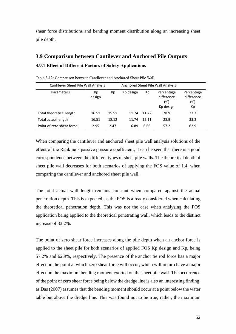
52

shear force distributions and bending moment distribution along an increasing sheet

pile depth.

3.9 Comparison between Cantilever and Anchored Pile Outputs

Effect of Different Factors of Safety Applications

Table 3-12: Comparison between Cantilever and Anchored Sheet Pile Wall

Cantilever Sheet Pile Wall Analysis Anchored Sheet Pile Wall Analysis

Parameters Kp design

Kp Kp design Kp Percentage difference

(%)

Percentage difference

(%) Kp design Kp

Total theoretical length 16.51 15.51 11.74 11.22 28.9 27.7

Total actual length 16.51 18.12 11.74 12.11 28.9 33.2

Point of zero shear force 2.95 2.47 6.89 6.66 57.2 62.9

When comparing the cantilever and anchored sheet pile wall analysis solutions of the

effect of the Rankine’s passive pressure coefficient, it can be seen that there is a good

correspondence between the different types of sheet pile walls. The theoretical depth of

sheet pile wall decreases for both scenarios of applying the FOS value of 1.4, when

comparing the cantilever and anchored sheet pile wall.

The total actual wall length remains constant when compared against the actual

penetration depth. This is expected, as the FOS is already considered when calculating

the theoretical penetration depth. This was not the case when analysing the FOS

application being applied to the theoretical penetrating wall, which leads to the distinct

increase of 33.2%.

The point of zero shear force increases along the pile depth when an anchor force is

applied to the sheet pile for both scenarios of applied FOS Kp design and Kp, being

57.2% and 62.9%, respectively. The presence of the anchor tie rod force has a major

effect on the point at which zero shear force will occur, which will in turn have a major

effect on the maximum bending moment exerted on the sheet pile wall. The occurrence

of the point of zero shear force being below the dredge line is also an interesting finding,

as Das (2007) assumes that the bending moment should occur at a point below the water

table but above the dredge line. This was found not to be true; rather, the maximum

53

bending moment for anchored sheet pile walls occurs at a point just below the dredge

line.

Effect of Different Factor of Safety Applications

The presence of the anchor tie rod force for anchored sheet pile walls decreases the

actual penetration depth below the dredge line dramatically. Applying the FOS to the

passive pressure coefficient results in a 63.52% decrease of actual penetration depth

below the dredge line, or a 65.89% decrease when the FOS is applied to the theoretical

penetrating depth below the dredge line (Table 3-13).

Table 3-13: Comparison between Cantilever and Anchored Sheet Pile Wall

Cantilever Sheet Pile Wall Analysis Anchored Sheet Pile Wall Analysis

Parameters Kp design

Kp Kp design

Kp Percentage difference

(%)

Percentage difference

(%) Kp design Kp

Actual Penetration Depth 7.51 9.12 2.74 3.11 63.52 65.89

Anchor Tie Rod Force - - 83.00 78.00 0.00 0.00

Maximum Bending Moment 787 741 209 180 73.43 75.72

Comparing the bending moment results for the cantilever sheet pile analysis with the

anchored sheet pile analysis results, it was found that the maximum bending moment

exerted on the sheet pile decreased substantially, with 73.43% for FOS applied to the

passive pressure and 75.72% for the FOS applied to the theoretical wall penetration

depth below the dredge line.

3.10 Conclusion

Designing sheet pile walls using the analytical methods is a very tedious and time-

consuming procedure. In the engineering industry, time is money, and a design tool that

could solve these equations automatically with the same accuracy and ability to create

visual solutions, all in a fraction of the time with only the necessity of inputting known

data, would be extremely valuable. The solutions obtained using the Excel spread sheet

are similar to those derived using the analytical methods. Thus, the Excel spread sheet

has been proven accurate and successful.

54

The analytical methods have been found to be conservative due to the necessity of

making several simplifications and assumptions. Important design information such as

ground settlement and possible surface failures cannot be obtained from the analytical

methods. It is thus proposed to use FLAC for future preferences to attain such critical

information to provide greater accuracy of results.

55

Chapter 4: FLAC Overview

4.1 Introduction

This chapter presents a short introduction to the FLAC software and explains the

necessary principles required for the use of this software. Several geotechnical

numerical modelling analyses were completed using FLAC. This chapter provides an

explanation of the FLAC program, highlighting its advantages and disadvantages for

undertaking the numerical analysis. This is important information for any designer

using numerical methods, as every software has its own limitations that need to be

recognised to enable a better understanding of particular outcomes.

FLAC is a 2D explicit finite difference program for engineering mechanics computation

(FLAC 2D online manual 2009). Explicit finite difference indicates the solution of the

problem being modelled by using a time-stepping procedure. FLAC contains a very

powerful built-in programming language called FISH (FLACish) that enables the user

to write single script files of code for increasing the usefulness and usability of this

software. The program simulates the behaviour of structures built of soil, rock or other

materials that may undergo plastic flow. These structures are described by the

behaviour of the elements according to a suggested linear or non-linear stress/strain

relationship (Das 1990).

Several different versions of FLAC are currently available, the most current of which

is version 6. For this dissertation, version 4 has been adopted due to its availability.

According to the establishment by Lyle (2009), there are only marginal differences

between the two versions, with the major difference being the speed improvements

obtained from FLAC version 6. This difference between the two versions would not

compromise the accuracy of the results. Thus, for the purpose of this dissertation, FLAC

2D was solely used to undertake the research. FLAC 2D indicates only two directions,

i and j, when undertaking the computations. Three-dimensional FLAC versions are

available; however, given the lack of time to learn a complex computer language, it was

decided to use the 2D version of FLAC.

56

4.2 Major FLAC Features

According to the FLAC manual, the FLAC software has a number of major features

(FLAC 2D online manual 2009):

Large strain simulations of continua, with optional interface that is able to

distinctively simulate planes along which slip and/or separation can occur.

Obtaining stable solutions from the provided explicit solution scheme when

compared to unstable physical processes.

Availability to model groundwater flow, with full coupling to mechanical

calculation (including negative pore pressure, unsaturated flow and phreatic

surface calculation).

Selection of multiple structural elements (including non-linear material

behaviour).

Full library of material models (e.g., elastic, Mohr-Coulomb plasticity,

ubiquitous joint, double-yield, strain-softening, modified Cam-Clay and Hoek-

Brown).

Statistical distribution of any property for generating plots of virtually any

problem variable with extensive facilitation.

Extra user-defined features such as the built-in language FISH (e.g., new

constitutive models, new variables or new commands).

To obtain a thorough understanding of FLAC programming, reasonable time and effort

is required. Experience is required to achieve accurate and effective results. Due to a

lack of experience using the program, it was necessary to carefully analyse all results

to ensure valid outputs. The results obtained from the FLAC software program will

therefore be validated as discussed in Chapter 5 to ensure quality solutions.

4.3 FLAC Model Analysis

The built-in programme language FISH gives the possibility to use the command-

driven software mode. Compared to the menu-driven mode in FLAC, the command-

driven mode was found to reduce the software’s performance of unnecessary repetitive

57

tasks, allowing for faster result assembly. The text file storing facility (known as a script

file) can be modified quickly and easily.

In the developed FLAC script based on the procedure outlined in Example 4.13 and

Installation of a Triple Anchored Excavation Wall in Sand (p 17-1) (FLAC 2D online

manual 2009), the basic steps undertaken to analyse cantilevered and anchored sheet

pile wall problems are as follows:

1. Create a mesh and define the various input variables for the mesh. Assume a

length for both horizontal and vertical direction. Define the number of blocks

per metre run. Specify the model Mohr of soil. (This model is the conventional

model used to represent shear failure in soils and rocks.) Input the soil properties.

2. Remove a complete column for the positioning of the sheet pile wall and shift

the right hand side block to the left with one single block difference to establish

a double coordinate system for creating an interface between the wall and the

soil.

3. Fix the boundary conditions to allow for possible horizontal collapse and

vertical displacement.

4. Specify the magnitude of gravity.

5. Insert the sheet pile wall and its specific properties.

6. Provide an interface between the pile and the soil on which sliding or separation

can occur. Attach the two sub grids created in step 2.

7. Set history to set small to avoid large settlement from occurring at the top of the

sheet pile. Solve the model elastically to reach equilibrium and save the current

state.

8. Reset all displacement back to zero before excavating the soil.

9. Excavate the soil on one side of the sheet pile, solve this process and save the

excavated state—hence the cantilever sheet pile wall model.

10. Install a cable structural element. Attach the cable element to the pile structure.

Specify the cable position and properties.

11. Solve the anchor sheet pile wall model and save the anchor model.

12. Save the graphical and numerical data produced during the solution phases of

FLAC into a specified folder.

58

FLAC Input Variables

Table 4-1: Grid Generation

X_Element size

Y_Element size

Grid size i,j

Table 4-2: Soil Properties

Bulk modulus (GPa) 3e9

Shear modulus (GPa) 1e9

Cohesion (𝑘𝑔/𝑚2) 0

Internal Friction Angle (degrees) 40

Dilation 0

Tension 0

Dry sand density (𝑘𝑔/𝑚3) 1922

Saturated sand density (𝑘𝑔/𝑚3) 2072

Effective sand density (𝑘𝑔/𝑚3) 1072

Table 4-3: Pile Element Properties (ArcelorMittal 2013; Das 2007)

Elastic Modulus of steel (GPa) 200

Area (𝑚2) 0.02

Second moment of inertia (𝑚4) 4.5e-6

Friction between Sand and Pile (degrees) 0

Penetration (D) depth of pile - cantilever (m) 9.12

Penetration (D) depth of pile – anchor (m) 3.11

Table 4-4: Rod Anchor Properties (Ischebeck; FLAC 2D online manual 2009)

Elastic modulus of steel (GPa) 200

Area (𝑚2) 0.0015

Yield strength (MPa) 1e10

Grout shear stiffness (MPa) 1e8

Intrinsic shear strength (MPa) 1e8

Friction between Tie Rod and Pile (degrees) 0

Tie rod length (m) 14

Tie rod element spacing (m) 1.2

Table 4-5: Solving Analysis

Solve elastic (obtain initial soil stresses)

Strain (set large or small)

Solve (before excavation)

Reset Displacement (y_disp = x_disp = 0)

Solve (after excavation)

Solve (after anchor installation)

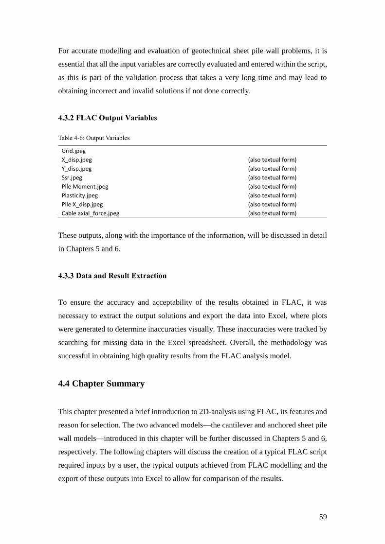
59

For accurate modelling and evaluation of geotechnical sheet pile wall problems, it is

essential that all the input variables are correctly evaluated and entered within the script,

as this is part of the validation process that takes a very long time and may lead to

obtaining incorrect and invalid solutions if not done correctly.

FLAC Output Variables

Table 4-6: Output Variables

Grid.jpeg

X_disp.jpeg (also textual form)

Y_disp.jpeg (also textual form)

Ssr.jpeg (also textual form)

Pile Moment.jpeg (also textual form)

Plasticity.jpeg (also textual form)

Pile X_disp.jpeg (also textual form)

Cable axial_force.jpeg (also textual form)

These outputs, along with the importance of the information, will be discussed in detail

in Chapters 5 and 6.

Data and Result Extraction

To ensure the accuracy and acceptability of the results obtained in FLAC, it was

necessary to extract the output solutions and export the data into Excel, where plots

were generated to determine inaccuracies visually. These inaccuracies were tracked by

searching for missing data in the Excel spreadsheet. Overall, the methodology was

successful in obtaining high quality results from the FLAC analysis model.

4.4 Chapter Summary

This chapter presented a brief introduction to 2D-analysis using FLAC, its features and

reason for selection. The two advanced models—the cantilever and anchored sheet pile

wall models—introduced in this chapter will be further discussed in Chapters 5 and 6,

respectively. The following chapters will discuss the creation of a typical FLAC script

required inputs by a user, the typical outputs achieved from FLAC modelling and the

export of these outputs into Excel to allow for comparison of the results.

60

Chapter 5: Numerical Analysis of Cantilever Sheet Pile Walls

5.1 Introduction

The objective of this chapter is to investigate the analysis of a cantilever sheet pile wall

penetrating a sandy type soil in the presence of a water table using the FLAC software.

The FLAC results will then be compared to the results from the Excel spread sheet

consisting of the analytical equations. The parameters that will be investigated within

the parametric study include:

fineness of mesh

effect of soil strength

effect of water table.

The variables such as the maximum bending moment, wall deflection and ground

settlement will be investigated.


Cantilever sheet pile walls are flexible structures. Due to the wall being flexible, when

the sheet pile wall moves away from the soil, it forms an active pressure zone; however,

when the wall moves into the soil, it forms a passive pressure zone (Figure 5.1). This

leads to the formation of pressure distributions on either side of the sheet pile wall.

Figure 5-1: (a) Cantilever Pile Penetrating a Sandy Soil, (b) Active and Passive Pressure Distribution

(Das 1990)

61

To obtain the total net pressure distribution exerted on the sheet pile wall, it is required

to add all the pressure distributions together.

For a design engineer, it is of upmost importance to determine the maximum bending

moment exerted on the sheet pile wall for structural design purposes and the net

pressure distribution exerted along the pile depth for stability purposes (Coduto 2001)

(Figure 5-2).

Figure 5-2: Cantilever Sheet Pile Penetrating Sand: (a) Net Pressure Variation Diagram; (b) Moment

Variation (Das 2007)

Based on the classical earth pressure theory, several methods commonly utilise the limit

state methodologies (e.g., the UK and USA methods) for analysing cantilever sheet pile

walls using the active and passive lateral pressures that act on the wall. The design

methods are based on the fact that force and moment equilibrium are required for

determining the minimum required wall penetration depth and the maximum bending

moment. A FOS should be applied to the passive pressures to take any uncertainties in

the soil condition, method of stability analysis and loading conditions into account, and

to restraint the soil movements to an acceptable level (Potts & Fourie 1984).

62

This dissertation’s investigations use FLAC software for undertaking a numerical

examination of cantilevered sheet pile walls as an alternative design analysis to the limit

equilibrium methods.

5.3 Problem Description

Figure 5-3 shows the problem to be investigated. The main parameters to be

investigated are the wall horizontal displacement, maximum bending moment and

ground settlement.

Figure 5-3: Problem to be Investigated

5.4 Analysis using FLAC

FLAC is a finite difference program and does not approach this problem in the same

way as the analytical methods. When using the limit equilibrium methods for solving

this problem, the penetration depth of the sheet pile is found to be below the dredge

line. Conversely, FLAC requires the penetration depth of the sheet pile to be entered

before it can be determined whether the system is stable. Thus, the overall soil/pile

system behaviour can be examined by varying several input parameters.

𝐿1 = 3 𝑚

𝛾 = 18.85𝑘𝑁

𝑚3

𝑐′ = 0

∅′ = 40°

D

𝐿1 = 6 𝑚


𝑚3

𝑐′ = 0

∅′ = 40°

Sheet Pile

Wall

Dredge Line

63

Creation of Model

The first step is to build the geometry of the problem, assuming an initial length in the

x and y directions. The soil layer boundaries and material properties are then defined.

Construction elements like walls and anchors are placed next. The soil/wall system is

then created using interface properties, which are then defined. Finally, the mesh is

generated. Over the years, several modes have been developed for representing the soil

behaviour. These include the linear elastic model, perfectly plastic model, hyperbolic

model and the Mohr-Coulomb model. Selecting the model to be used for modelling the

soil is extremely important and is dependent on several factors, as specified by

Ramadan (2013). Initially, a very course mesh was assumed to analyse the specific

problem (Figure 5-4). This was adjusted upon gaining a greater familiarity with the

FLAC software.

Figure 5-4: Assumed Course Mesh Grid

Soil Mass Properties

The soil acts as non-linear and irreversible when subjected to very high loads.

According to FLAC 2D online manual (2009), a number of constitutive models are

available, as FLAC is able to distinguish between several material models for soil,

interfaces, plates, anchors and geogrids. The numerical analysis that was performed

20 elements, 25 m

18 e

lem

ents

, 22

m

64

analysed the soil under drained soil conditions and suggested that pore water pressure

could be prevented from developing. Normally, this drainage type is used for dry soils

for accommodating full drainage due to high permeability. In FLAC, there are two

options for modelling the soil mass:

The initial stresses within the soil mass can be set. This initial stress condition

depends on the weight of the material and the history of the formation. The

stress state at that initial moment is characterised by a vertical effective stress

(𝜎𝑣′), whereas the horizontal earth pressure is determined by the lateral earth

pressure (or at rest) coefficient (𝐾0).

All of the above recommendations may be ignored if and only if the soil mass

is solved to reach equilibrium using the ‘solve elastic’ at the first instance, thus

automatically creating the initial stresses due to the weight of the soil mass.

Construction of Sheet Pile

The sheet pile was constructed by inserting a structural beam element into the mesh.

The surface of this sheet pile was modelled as perfectly smooth so as not to form any

friction between the soil and the sheet pile. This was done to ensure accuracy when

comparing the numerical results with the analytical solutions. (A frictionless effect

between the sheet pile wall and soils was originally assumed by Das [2007].) The sheet

pile wall properties were specified according to ArcelorMittal (2013) a leading steel

manufacturing company. These properties were specified in Chapter 4.

65

To create this interface between the pile and the grid, it was required to remove a

complete column (Figure 5-5) where the pile would be constructed using the ‘model

null’ command to generate a double coordinate system to which to attach the pile.

Figure 5-5: Column Removed for Sheet Pile Construction

The sub grid on the right then had to be incrementally moved to the left according to

the grid ratio as specified by the user. The sheet pile was then installed, as shown in

Figure 5-6.

Figure 5-6: Constructed Sheet Pile Wall Model

20 elements, 25 m

18 e

lem

ents

, 22

m

19 elements, 23.7 m

18 e

lem

ents

, 22

m

66

Interface Properties

According to the FLAC manual, an interface between the soil/wall systems is

represented as normal, and there is shear stiffness between the two planes (Figure 5-7).

For either side of the interface, FLAC uses contact logic similar to that used by the

finite element method.

Figure 5-7: An Interface Represented by sides a, and b, connected by shear (𝒌𝒔) and normal (𝒌𝒏) stiffness

springs (FLAC 2D online manual 2009)

The code keeps a list of the grid points (𝑖, 𝑗) that lie on each side of any particular

surface. Each point is then taken and checked for contact with its closest neighbouring

contact point on the opposite side of the interface. Referring to Figure 5-6 on the

segment M-P, the grid point marked N is checked for contact between the specified

segment. The length LN is defined for the contact of N between the segment M-P. The

length is equal to half the distance to the nearest grid point to the left of N, plus half the

distance to the nearest grid point to the right, irrespective of the side on which the

neighbouring grid point is located. This will ensure that the entire interface is divided

into contiguous segments, each controlled by a grid point. The interface was thus

successfully installed, creating a valid interface between sub grids and between the

element and the grid.

67

Soil Excavation

The required depth above the dredge line to the left of the sheet pile was then excavated

using the same ‘model null’ command.

Figure 5-8: FLAC Model Containing Course Mesh

After excavating the soil, the model was solved again using the ‘solve’ command to

investigate the effects and behaviour of the sheet pile wall by interpreting specific

FLAC outputs such as maximum bending moment, maximum wall horizontal

deformation and failure surface.

FLAC Results

Establishing whether the created model is correct forms part of the model validation

process. This process is time consuming for unexperienced FLAC users and might be

frustrating; however, being able finally to interpret correctly the outputs obtained from

FLAC is extremely rewarding.

19 elements, 23.7 m

18 e

lem

ents

, 22

m

9 m

9

.12 m

68

Failure Surface

Plotting the failure surface on a shear strain rate plot gives a good indication of whether

the grid size of the model is acceptable.

Figure 5-9 (a) is the initially assumed model grid. The failure surface in Figure 5-9 (b)

is not fully contained within the initially assumed grid. Thus, it was required to increase

the grid in the x-direction (that is, widen it in the horizontal direction).

Figure 5-9: (a) Grid, (b) Failure Surface for initially assumed Model

25 m 25 m

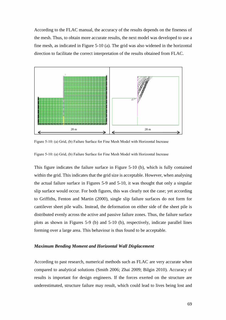
69

According to the FLAC manual, the accuracy of the results depends on the fineness of

the mesh. Thus, to obtain more accurate results, the next model was developed to use a

fine mesh, as indicated in Figure 5-10 (a). The grid was also widened in the horizontal

direction to facilitate the correct interpretation of the results obtained from FLAC.

Figure 5-10: (a) Grid, (b) Failure Surface for Fine Mesh Model with Horizontal Increase

Figure 5-10: (a) Grid, (b) Failure Surface for Fine Mesh Model with Horizontal Increase

This figure indicates the failure surface in Figure 5-10 (b), which is fully contained

within the grid. This indicates that the grid size is acceptable. However, when analysing

the actual failure surface in Figures 5-9 and 5-10, it was thought that only a singular

slip surface would occur. For both figures, this was clearly not the case; yet according

to Griffiths, Fenton and Martin (2000), single slip failure surfaces do not form for

cantilever sheet pile walls. Instead, the deformation on either side of the sheet pile is

distributed evenly across the active and passive failure zones. Thus, the failure surface

plots as shown in Figures 5-9 (b) and 5-10 (b), respectively, indicate parallel lines

forming over a large area. This behaviour is thus found to be acceptable.

Maximum Bending Moment and Horizontal Wall Displacement

According to past research, numerical methods such as FLAC are very accurate when

compared to analytical solutions (Smith 2006; Zhai 2009; Bilgin 2010). Accuracy of

results is important for design engineers. If the forces exerted on the structure are

underestimated, structure failure may result, which could lead to lives being lost and

28 m 28 m

70

the design engineer being held accountable. By analysing the cantilever sheet pile wall

behaviour in FLAC, it was possible to obtain the maximum bending moment exerted

on the sheet pile wall and the maximum horizontal wall displacement. As already

mentioned, these outputs are extremely important for stability and structural design

purposes (Figure 5-11).

Figure 5-11: (a) Maximum Bending Moment, (b) Maximum x-Displacement

Containing these visual outputs certainly gives a good indication of the soil-wall

system; however, determining the quality of the result outputs is what is important. This

validation is done by comparing the FLAC output of maximum bending moment with

the maximum bending moment obtained from the limit equilibrium methods as

established in Chapter 3. Unfortunately, the maximum wall horizontal deflection cannot

be validated, as this deflection cannot be obtained from the limit equilibrium methods.

This is a limitation of using the analytical methods.

610 𝑘𝑁.𝑚

449 𝑚𝑚

71

Soil Mass Failure

The failure of the soil mass can be examined by plotting the plasticity graph in FLAC

(Figure 5-12). This plot indicates which elements are at yield or have undergone plastic

deformation. The green elements indicate at yield elements undergoing elastic

deformation, while the red elements indicate elements undergoing plastic deformation.

Figure 5-12: Plasticity Indicators for the Fine Mesh Model

The overall purpose of analysing this plot is to determine whether the system fails. It is

thus crucial to examine the plot of plasticity indicators for each element prone to failure.

The soil mass is found to fail when the plasticity elements on one side of the sheet pile

connect the ground surface to the ground surface on the other side of the sheet pile via

extending around the sheet pile tip. Failure also occurs when the plastic elements extend

far beneath the sheet pile tip into the outer boundary of the plot.

By examining Figure 5-12, it is clear that this sort of behaviour is not occurring. Thus,

it is reasonable to conclude that the cantilever sheet pile wall penetrating 18.12 m of

sandy soil is safe, as failure is not occurring.

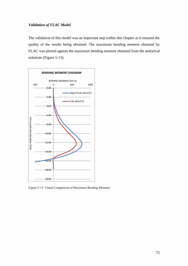
72

Validation of FLAC Model

The validation of this model was an important step within this chapter as it ensured the

quality of the results being obtained. The maximum bending moment obtained by

FLAC was plotted against the maximum bending moment obtained from the analytical

solutions (Figure 5-13).

Figure 5-13: Visual Comparison of Maximum Bending Moment

0.00

2.00

4.00

6.00

8.00

10.00

12.00

14.00

16.00

18.00

20.00

-500 0 500 1000

WA

LL P

ENET

RA

TIO

N D

EPTH

(m

)

BENDING MOMENT (kN.m)

BENDING MOMENT DIAGRAM

ANALYTICAL RESULTS

FLAC RESULTS

73

As shown in Table 5-1, the maximum bending moment obtained from FLAC sees only

a 17.67% reduction from the maximum bending moment obtained using the analytical

methods. This gives a 82.32% comparison between the obtained solutions.

Table 5-1: Comparison of Maximum Bending Moment

Wall total Analytical FLAC Solution Percentage

Depth (m) Solution Solution Reduction (%)

17.8 741 610 17.67

This close comparison indicates that the results compare very well, strongly suggesting

the validity of the results obtained from FLAC. The maximum bending moment

obtained from FLAC is also smaller than the value obtained when using the analytical

methods, indicating that the FLAC results are more accurate than are those obtained

using the analytical solutions. Thus, the assumptions made by the analytical methods

lead to the results being more conservative. To ensure complete validation of the model,

it was necessary to validate the wall horizontal deformation and the ground surface

settlement values obtained in FLAC against previously conducted work (Table 5-2).

Table 5-2: Validation of FLAC Model

Wall Penetration Depth D (m)

Maximum Wall Deflection (m)

Maximum Surface Settlement (m)

Percentage Correspondence (%)

6.88 0.984 1.65 59.63

7.57 0.780 1.23 63.41

8.08 0.667 1.00 66.70

8.60 0.545 0.812 67.11

9.12 0.459 0.662 69.33

Similar to previous research it was found that as the wall penetration depth increases

both the maximum wall deflection and the maximum surface settlement decreases thus

indicating a non-linear relation occurring. The percentage correspondence between the

maximum wall deflection and maximum surface settlement thus linearly increases due

to the non-linear relationship between the values as this is expected, since a closer

correspondence would occur when values become smaller leading to a smaller

difference and thus increasing the accuracy of the results.

This finding proves that this cantilever model is both valid and produces quality results.

74

Convergence Study

The parametric study focusses primarily on studying the effect of changing the mesh

fineness to investigate the effect on the model accuracy. Varying the friction angle of

the sandy soil to analyse how the soil strength affects the behaviour of the sheet pile

wall. Inspecting the water table effect with varying sheet pile wall depth analysing the

behaviour of the sheet pile by analysing the outputs such as the wall deformation,

bending moments and ground settlement computed in FLAC.

Effect of Mesh Fineness

According to the FLAC manual, the accuracy of the results depends on the fineness of

the mesh. Analysing a model containing a fine mesh will result in accurate solutions.

As can be seen from Table 5-3, this is definitely the case as the mesh was increased

from course to fine the maximum bending moment obtained for models containing

medium and fine meshes respectively was smaller than compared to the maximum

bending moment obtained by the analytical solutions.

Table 5-3: Convergence Study of Varying Mesh Fineness

Mesh fineness Maximum bending moment (kN.m)

Maximum wall deflection (m)

Maximum surface settlement (m)

Blocks per m run

Course 837 0.678 0.830 80

Analytical Solution 741 - - -

Medium 680 0.503 0.688 100

Fine 610 0.459 0.662 120

Analysing the maximum bending moment obtained from the model containing a course

mesh, a much larger value is obtained compared to analytical solutions. This indicating

that the results obtained from FLAC are more conservative than the analytical solutions.

This is quite strange and it might lead to the thought that the results are invalid. For

unexperienced FLAC users this might be the case. This indicates that using such course

meshes to model numerical geotechnical problems should be avoided as this may lead

to inaccurate solutions. It is best to undertake modelling using a medium mesh and

increasing the fineness from thereon. Therefore, the findings emphasise the importance

for the necessity of skilled FLAC users when undertaking numerical analysis

modelling.

75

Investigating the maximum wall deformation and maximum ground settlement only the

results obtained from the medium and fine mesh will be taken into consideration as we

have established the data from modelling with a course mesh may be misleading.

The maximum wall deformation increases with the increase of the mesh fineness,

indicating a direct relation occurring. As mentioned in previous chapters obtaining

accurate maximum wall deformation data is important for serviceability purposes as

this information is used by engineers to determine if the structure satisfies serviceability

requirements.

The maximum ground settlement increases with the increase of mesh fineness once

again leading to more accurate results. The accuracy of the maximum ground settlement

result is important as the ground settlement effects nearby structures. Normally, in

urban environments, excavation occurs nearby other structures. If the maximum ground

settlement effect has not been investigated, catastrophic building collapses may result.

Effect of Soil Friction Angle

An additional analysis was performed using relatively looser and denser sandy soils to

investigate the effect of soil strength on the sheet pile wall behaviour with increasing

wall penetration depth below the dredge line.

The analysis results, in terms of maximum wall displacement and maximum bending

moments, for a loose sandy soil (∅ = 35°), medium dense sandy soil (∅ = 40°) and a

very dense sandy soil (∅ = 45°) are given in Table 5-4.

Table 5-4: Parametric Study of Soil Friction Angle

FLAC Analysis Analytical Analysis

Soil Friction Angle (degrees)

Penetration Depth D (m)

Maximum Bending Moment (kN.m)

Maximum Wall Deflection (m)


35 10.68 935 0.825 1034

40 9.12 610 0.459 741

45 7.85 394 0.250 535

76

The reduction of the maximum bending moment obtained by FLAC is relative to the

conventional design method values. The maximum bending moment results obtained

from FLAC compared to the solutions obtained by the analytical solutions are smaller,

thus ensuring high quality results were obtained.

The cantilever sheet pile has less wall deformation for denser soils with decreasing

penetration depth below the dredge line. This is very interesting as earlier determined

for decreasing penetration depth the wall deformation increases, but increasing the soil

strength leads to the opposite behaviour occurring. As the penetration depth below the

dredge line decreases, the wall deflection also decreases with increasing soil strength

of the soil.

Effect of the Ground Water Table

Often, sheet pile structures are built-in connection with waterfront facilities. The effect

of hydrostatic pressure should be added to the earth pressure if the soil is not able to

drain the water from behind the sheet pile wall. If the water level varies on either side

of the sheet pile wall an unbalanced hydrostatic pressure is formed leading to increasing

lateral pressure that may cause the wall to be forced in an outward direction. In Figure

5-2, the water table on both sides of the sheet pile wall is presented at the same level as

suggested by Das (2007). This leads to the soil being fully submerged, causing the

hydrostatic pressures at any depth from both sides of the wall to cancel out, therefore

only considering the effective lateral soil pressures exerted on the wall below the water

table.

77

As shown in Table 5-5, the maximum bending moment for the cantilever sheet pile wall

model containing no water table is 23.29% larger than the maximum bending moment

obtained from the cantilever sheet pile wall model with a water table present. This was

expected due to the assumption made by Das.

Table 5-5: Parametric Study of Ground Water Table

No Water Table Model Water Table Model

Wall Penetration Depth D (m)



Percentage Decrease (%)

6.64 717.00 550.00 23.29

7.00 627.00 497.00 20.73

7.55 479.00 394.00 17.74

It was assumed that the hydrostatic pressures on either side of the wall cancelled each

other out, however the effective unit weight of a soil should be used in the presence of

a water table. Thus obtaining a much smaller effective unit weight of the soil when

compared to the normal unit weight of the soil, which was used for the model in the

absence of the water table. Decreasing bending moment occurs for the increase of

penetration depth below the dredge line, forming a direct relationship. It is completely

acceptable for the model in the absence of a water table to expect a larger maximum

bending moment exerted on the pile, due to the large soil force exerted on the pile.

Chapter Summary

The wall behaviour was investigated through the wall displacements, bending moments

and ground settlement. The finite difference method, FLAC was used to analyse this

sheet pile wall behaviour and to investigate the effect of a changing specific parameters

and undertaking a parametric study to investigate the behaviour of the pile.

It was obtained that using finer mesh grids led to more accurate results as well as being

able to obtain outputs that can easily be analysed thus leading to more qualitative

results. It is of upmost importance to have skilled FLAC user, model geotechnical

engineering problems to be able to understand the outputs obtained from FLAC as well

as validating the model. As validating the model is the most critical part of numerical

modelling, the results were validated by comparing the solutions to the obtained

analytical solutions. To find once again that the results obtained from FLAC are very

78

accurate when compared to the analytical solutions. This could have been expected as

many assumptions were made by Das to simplify the tedious analytical equations,

creating more conservative solutions.

For higher density sandy soils (that is, stronger soil), a reduction was found in the total

wall displacement, with decreasing wall penetration depth below the dredge line

leading to a dramatic reduction of the maximum bending moment.

The effect of the water table leads to decreasing maximum bending moment values

when compared to absent water table models. Due to the simplifications and

assumptions made by Das, the hydrostatic pressures on either side of the wall cancel

each other out. A larger soil mass with normal unit weight will produce larger lateral

forces exerted on the sheet pile wall than compared to a smaller soil mass only

containing an effective unit weight of the soil producing smaller pressures exerted on

the pile. Hence, the increase of maximum bending moment with reduced wall

penetration depth is completely acceptable.

79

Chapter 6: Numerical Analysis of Anchored

Sheet Pile Walls

6.1 Introduction

The objective of this section of the project is to use FLAC to investigate the complex

anchored sheet pile wall penetrating sand problem. The investigation includes a

parametric study to examine how certain parameters may have an influence in

producing more cost beneficial sheet pile walls in the engineering industry. The

parameters to be investigated include:

Adding an anchor to high cantilever sheet pile walls

Varying depth effect


There are several traditional design methods used to design anchored sheet pile walls

like the free earth and fixed earth support methods (Das 2007). For complicated

problems including the construction effect on the pile-soil system, computer programs

are used to analyse the behaviour of the sheet pile. Many researchers have shown over

the years that designing sheet pile walls when using the free earth support method

provide stable sheet pile walls with less wall penetration depth below the dredge line

required. Therefore, when using the fixed earth support methods lower wall deflections

are predicted for less stable piles when compared to the free earth support methods.

There are, however, multiple ways of reducing the large wall deformations obtained

when using the free earth support method stated by (Erten & Bilgin 2009) to make use

of multiple anchorage systems to be the most effective but also using larger pile profiles

than required by the analytical design methods can also be very effective.

80

6.3 Problem Description

The geotechnical problem specifies a sheet pile wall penetrating a sandy soil to a 3.11

m depth below the dredge line (Figure 6-1).

Figure 6-1: Problem to be investigated

The main parameters that will be investigated are the sheet pile wall horizontal

displacement, maximum bending moment exerted on the sheet pile wall and the ground

settlement.

6.4 Analysis using FLAC

The conventional analytical methods do not take into consideration the construction

effect when installing the structural elements such as the sheet pile and anchor tie rod.

The analytical design methods do not consider the properties of the structural elements.

This leads to the development of limitations being present when using these analytical

methods. To obtain more accurate sheet pile wall designs, numerical analysis in FLAC

is undertaken.

𝐿1 = 3 𝑚

𝛾 = 18.85𝑘𝑁

𝑚3

𝑐′ = 0

∅′ = 40°

D

𝐿2 = 6 𝑚


𝑚3

𝑐′ = 0

∅′ = 40°

Anchor Force 𝑙1 = 1.5 𝑚

𝑙2 = 1.5 𝑚

Dredge Line

Sheet Pile Wall

81

Model Creation

The boundary of the specific sheet pile wall problem has already been established and

validated in Chapter 5. Therefore, it was only necessary to install or construct the

grouted tie rod anchor element to create an anchor sheet pile model in FLAC using the

fine mesh grid (Figure 6-2).

Figure 6-2: Anchor Sheet Pile Wall Model

Modelling of Anchor Element

Cable elements are one-dimensional axial elements that may either be anchored at a

specific point in the grid (point anchored), or grouted so that the cable element develops

forces along its length as the grid deforms. Cable elements can yield in tension or

compression, but they cannot sustain a bending moment. If desired, cable elements may

be initially pre-tensioned. Cable elements are used to model a variety of supports,

including rock bolts, cable bolts and tiebacks.

28 m

9 m

3

.11 m

7.51 m

82

A node-to-node anchor system containing of a two-node elastic spring element with

constant spring stiffness (normal stiffness) is created to model typical anchor sheet pile

wall applications (Figure 6-3).

Figure 6-3: Node-to-node Anchors (Ramadan Amer 2013)

FLAC Results

Several output plots are investigated in this section. Outputs defined as the surface

failure, plastic-elastic deformation, maximum bending moment, structure horizontal

displacement and ground settlement will be inspected. Even though the cantilever

model responses have been discussed in detail in Chapter 5, a new cantilever model

was developed with the same penetration depth below the dredge line as required for

the anchor model for the ability to compare the anchored sheet pile model results with

the results obtained from the cantilever sheet pile wall model. This has been provided

to establish the differences and agreements between the two types of pile models.

6.4.3.1 FLAC Model Validation

In engineering design procedures information such as the bending moment distribution

exerted along the sheet pile wall is important information to consider for structural

design purposes. The developed anchor sheet pile wall model has to be validated before

further parametric studies can be done using this model. The anchor sheet pile wall

model was validated by comparing the FLAC results with analytical solutions and

observations from previous studies.

83

The design of anchored sheet pile walls in a sandy soil has to satisfy the following:

1. The sheet pile should be stable after the construction of the wall (ultimate limit

state).

2. The displacements and deformations of the sheet pile wall should be small so

that the sheet pile wall will function as intended in the design (serviceability

limit state).

3. Settlements and lateral displacements caused by the installation process of the

structural elements should be small so that adjacent buildings or other nearby

structures are not damaged.

To validate the anchor sheet pile wall model created in the FLAC software program, it

was necessary to compare the solutions obtained from the numerical modelling with

the analytical solutions found from using the limit equilibrium methods (Figure 6-4).

Firstly, the maximum axial anchor tie rod force between the numerical and analytical

methods was distinguished.

Figure 6-4: Visual Comparison of Maximum Anchor Tie Rod Force

Both the analytical and numerical data for the axial anchor tie rod force increases

gradually until a maximum is reached then the force strength decreases slowly. It has

been found that the maximum axial force obtained when using the numerical methods

is 14.37% smaller when compared to the analytical solution for the anchor tie rod force.

This indicates that the results obtained from FLAC, where the structural properties has

been considered give a more realistic and accurate indication of the anchor tie rod force

behaviour along the specified length.

0

10

20

30

40

50

60

70

80

90

0 1 2 3 4 5 6 7 8

AN

CH

OR

FO

RC

E (

kN

)

ANCHOR ROD LENGTH (m)

MAXIMUM AXIAL ANCHOR FORCE

FLAC DATA

ANALYTICAL DATA

84

Similarly, the bending moment distribution along the sheet pile wall for both analytical

and numerical analysis has been plotted along the increasing sheet pile wall depth

(Figure 6-5).

Figure 6-5: Visual Comparison of Maximum Bending Moment

After analysing the cantilever sheet pile solutions, it was assumed that similar results

would be obtained for the anchor sheet pile. The visual representation gives a good

understanding of how the analytical methods exaggerate the solutions when compared

to the numerical solutions. This visual representation of the analytical plot of maximum

bending moment is misleading as the anchor sheet pile will not necessarily behave in

such a way in a ‘real life’ situation. Figure 6-5 indicates a reduced comparison between

the analytical and numerical solutions.

0

2

4

6

8

10

12

14

-200 -100 0 100

WA

LL

PE

NE

TR

AT

ION

DE

PT

H (

m)

BENDING MOMENT (kN.m)

MAXIMUM BENDING MOMENT DIAGRAM

FLAC RESULTS

ANALYTICAL RESULTS

85

The numerical solutions indicate that the analytical methods are very conservative when

compared to the numerical solutions. FLAC is able to produce more accurate results of

the soil-structure system behaviour, ensuring more accurate sheet pile wall designs in

the engineering industry (Table 6-1).

Table 6-1: Comparison of Maximum Bending Moment

Wall Total Depth (m)

Cantilever Sheet Pile Anchored Sheet Pile Percentage

Numerical Solution Analytical Solution

Numerical Solution

Reduction (%) Numerical

Reduction (%) Design Methods

12.11 45.16 174.26 29.36 34.98 83.15

The discovery in Chapter 5 provided the maximum bending moment obtained from the

numerical methods to be very accurate compared to the analytical methods. In order to

be able to compare solutions between cantilever and anchor models, it was necessary

to create a cantilever model with the same penetrating depth below the dredge line as

for the established anchor model to establish the effect of the installation of an anchor

to a cantilever sheet pile.

It was found that the maximum bending moment decreased with 76.48% after the

installation of the anchor tie rod to the cantilever sheet pile wall. The presence of the

anchor force as also changed the effect of the bending moment on the sheet pile for a

depth of 1.5 m below the surface from a negative to a positive bending moment,

showing a decrease of 34.98% at 1.5 m. The installation of anchors proves to have

sufficient effect on the structural integrity of the sheet pile wall system.

Comparing the maximum bending moment solution obtained from the analytical

methods with the numerical FLAC software, the maximum bending moment decreases

83.15%. This is a very large decrease, which indicates that the results obtained do not

compare well with each other. This is due to the assumption that no pivot point exists

for the static system when using the free earth support method (Das 1990). The results

indicate that assumption have major impacts on the outputs and solutions. The

assumption of the absence of the pivot point was not considered when analysing the

maximum bending moment exerted on the anchored sheet pile in FLAC.

86

FLAC, however, analyses the anchor sheet pile problem as a ‘real life’ situation, where

different lateral soil pressures may lead to the existence of a pivot point on the sheet

pile. Although the analytical and numerical results do not compare well, the net bending

moment behaviour along the sheet pile is proven acceptable by comparing the

numerical results obtained in FLAC, with finite element analysis results (Woods 2003).

Failure Surface

The failure surface will be analysed more in depth for this particular chapter as the basic

understanding of obtaining and examining the failure surface plots has been established

in Chapter 5 for a cantilever sheet pile wall problem. Due to specimen weakness or

imperfect boundary conditions, inhomogeneous deformations occur and strains thus

become concentrated into narrow zones, also known as ‘shear bands’.

Figure 6-6: Failure Surface Plots; for (a) Cantilever Pile, (b) Anchored Pile

The failure surface within the soil mass for both cantilever and anchored sheet pile wall

models similarly consists of distinct parallel slip surfaces. However, there is a slight

change between these two figures. The shear bands obtained from the cantilever sheet

pile model indicates one directional shear plane behaviour, whereas the anchor sheet

pile model obtains multidirectional shear band occurrence. The occurrence of these

shear bands consisting of thin multilayers are bounded by two material discontinuity

surfaces of a velocity gradient.

12.1

1 m

12.1

1 m

87

This is due to the Mohr-Coulomb criterion that indicates the friction angle of the soil

defines the maximum ratio of the shear stress to normal stress than can be mobilised in

cohesion less soil (Sadrekarimi & Olson 2010). A specific shear band will form in the

direction of the plane on which this friction angle is mobilised. At failure, this plane is

inclined at an angle of (45 −∅

2 ) with respect to the direction of 𝜎1 and is termed the

Coulomb rapture plane (Sadrekarimi & Olson 2010).

The shear bands specified for both the cantilever and anchored sheet pile wall models

are much larger than the failure point of 25°, thus the shear bands do not represent

failure of occurring for the above-developed models. The cantilever sheet pile wall

surface failure plot contains shear bands with smaller band thickness.

The reason for this occurrence is due to the large soil mass acting laterally towards the

cantilever sheet pile, whereas this action is counter balanced by the anchor force in the

anchor sheet pile wall failure surface plot, resulting in the thicker shear bands. It was

found that the width of the shear bands is not affected by any geometrical dimensions

of a soil body other than its grain size (Vardoulakis 1987). This is an important

phenomenon when analysing the progressive failure in granular soils.

Soil Mass Failure

As mentioned briefly in Section 5.4.6 FLAC Results, the failure of the soil mass can be

examined by plotting the elastic-plastic deformation plot. The fundamental assumption

of the Elastic-Plastic Soil Mechanism is that strains can be separated into two main

components, a recoverable elastic strain component and an irrecoverable plastic strain

component. In notation form this is written as 𝜀𝑣 = 𝜀𝑣𝑒 + 𝜀𝑣

𝑝 for volume strain and,

similarly, for shear strain as 𝜀𝑠 = 𝜀𝑠𝑒 + 𝜀𝑠

𝑝.

88

Comparing the elastic-plastic plots for cantilevered sheet pile walls with the anchored

sheet pile wall model, it can be seen that the red elements, which indicate elements

undergoing plastic deformation is connecting the ground surface on one side of the

sheet pile wall to the ground surface on the other side of the sheet pile wall (Figure 6-

7). This indicates that the soil mass is failing due to the mechanism called shallow shear

failure.

Figure 6-7: Plasticity Indicators; (a) Cantilever Model, (b) Anchor Model

Similarly, the same is occurring for the anchored sheet pile wall model; however the

failure incident is due to possible rotational failure. The combination of both plastic and

elastic elements occurring at the same time indicates that the applied stress is greater

than the current yielding surface, predicted that the strains will have both elastic and

plastic components. When a combination of stresses greater than the yield surface is

applied, plastic strains develop in response to this stress and enlarge the yield surface

to include the current stress state. The strength law describes this scenario as the stress

state where the material fails. The reason for this failure occurring is assumed to be due

to the very small penetration depth of the sheet piles beneath the dredge line. It was

therefore found interesting to undertake a parametric study of varying the depth of the

sheet pile below the dredge line, to establish whether this was the main cause of failure.

It can also be noted when comparing the size of the surface area existing of the

plastically deformed elements for the cantilever and anchor elastic-plastic plots that a

larger plastically deformed surface area is obtained for the cantilever sheet pile wall

89

than for the anchored sheet pile wall model. This indicates that the anchor tie rod force

has decreased the surface area of the plasticity, thus reducing the stress.

It is important to note for both sheet pile models that there is no indication of plastically

deformed elements extending far below the tip of the sheet pile. Thus the sheet pile wall

is not undergoing structural failure (Jardine et al. 1986).

Parametric Study

A large number of factors affect the behaviour of anchored sheet pile walls. In this

dissertation, experience with sheet pile walls primarily penetrating sandy soil have been

reviewed. FLAC has been used to determine the stability of an anchored sheet pile wall

under large excavation. The sheet pile penetration depth will be increased four times to

analyse the effect on the sheet pile response and determine methods for increasing the

stability of anchored sheet pile walls undergoing large excavations.

The parametric study results were performed to investigate the effect of increasing the

wall penetration depth on the anchored sheet pile wall behaviour in a sandy soil. The

analysis results in terms of maximum total wall displacement, maximum bending

moment, maximum ground settlement and anchor forces with increasing wall depth

(Table 6-2).

Table 6-2: Maximum Bending Moment, Maximum Wall Displacement, Maximum Ground Settlement,

and Anchor Forces with Increasing Wall Penetration Depths

Normalised Penetration Depth (D/H)

Wall Penetration

Depth, D (m)

Maximum Wall Displacement

(m)

Maximum Ground Settlement (m)

Maximum Wall Bending

Moment (kN.m)

Anchor Tie Rod Force (kN)

0.34 3.11 0.297 0.500 38.26 64.57

0.44 4.00 0.235 0.386 37.56 64.36

0.56 5.00 0.226 0.321 36.97 64.25

0.67 6.00 0.188 0.305 32.54 64.18

0.77 7.00 0.173 0.289 29.95 63.82

The results indicate that as the penetration depth of the sheet pile wall below the dredge

line increases the maximum horizontal wall displacement decreases. There is a very

good relation between the values of maximum wall displacement. This can be expected,

90

as the position of the anchor tie rod force did not change. The ground settlement also

indicated an indirect behaviour of decrease with increasing pile penetration depth.

These results are similar when compared to the solutions obtained from the cantilever

sheet pile wall models.

The maximum bending moment for the anchored sheet pile wall, decrease with an

increase of sheet pile penetration depth. This indicated that the system became more

stable as the penetration depth increased. Therefore, the initial assumption of both the

cantilever and anchor sheet piles undergoing material failure as indicated on the

plasticity plots was due to the insufficient sheet pile wall penetration depth. The anchor

axial force results indicate a slight decrease of anchor force with respect to an increasing

penetration depth. The direct relationship between the decreasing maximum bending

moment and anchor force is expected, as the position of the anchor force was not

altered.

Chapter Summary

The effect of increasing the wall penetration depth showed a significant effect on the

behaviour of the anchor sheet pile wall maximum bending moment and the failure of

the entire pile-soil system. However increasing the sheet pile penetrating depth will

increase the cost of installing sheet pile walls.

To conclude this chapter it was found that the anchor sheet pile required a sheet pile

wall length increase beneath the dredge line in order to obtain a safe pile-soil system.

Unfortunately, due to time constraints, further parametric studies analysing the effect

of placing the anchors at an inclined angle and varying the depth of the anchor force

placement position to find a cost-effective solution for sheet pile wall designs in the

industry could not be undertaken.

However, the anchor sheet pile wall model that has been created in this dissertation

proves sufficient due to delivering accurate results when compared to the analytical

method and cantilever sheet pile wall model solutions, as fewer assumptions were made

when undertaking the numerical anchored sheet pile problem. The numerical model

91

developed in FLAC was validated by comparing the sheet pile wall behaviour with

solutions obtained by (Woods 2003).

92

Chapter 7: Conclusions

This chapter summarises the outcomes of this research project and discusses the

achievements of the project and recommendations for areas of future work.

7.1 Spread Sheet Development for Sheet Pile Wall Design

Designing sheet pile walls using the limit equilibrium methods and finding solutions

by means of hand calculations is time consuming and prone to human error. In the

engineering industry, time is money, so the development of an automatic sheet pile

design tool that could solve the tedious analytical equations accurately and create visual

solutions, all in a fraction of the time and with only the necessity of inputting known

data, would be highly valuable.

The solutions obtained using the Excel spread sheet are similar to the solutions derived

from the analytical methods. Thus, the Excel spread sheet has proven both accurate and

successful.

However, these analytical methods of design have been found very conservative due to

making several simplifications and assumptions. For example, important information

such as ground settlement and possible surface failures cannot be obtained from the

analytical methods. Thus, it is proposed to use available industrial software such as

FLAC to attain critical information and provide greater accuracy of results.

7.2 Cantilever Sheet Pile Wall

The cantilever sheet pile wall was successfully researched, including methods of

solution and design. The wall behaviour was investigated through the wall

displacements, bending moments and ground settlement. FLAC was used to analyse

this sheet pile wall behaviour, investigate the effect of changing specific parameters

and undertake a parametric study to investigate the behaviour of the pile in certain

situations.

93

Many valuable conclusions have been drawn. For example, using a very fine mesh

when examining the numerical models leads to very accurate results. Examining the

results correctly when modelling geotechnical problems in FLAC using course mesh

grids is quite challenging, as the results may be misleading. Therefore, numerical

models using course mesh grids should be avoided. This emphasises the importance of

having a skilled FLAC user undertake the numerical modelling and evaluate the outputs.

A parametric study was implemented to investigate the effect of a change in soil density

and the presence of a water table below the ground surface. Such parametric studies

illustrate possible ‘real life’ situations. Testing models in this way indicates the

possibility of using these numerical models in the engineering industry to find optimum

designs and save engineering companies unnecessary expense by providing an

alternative to the design of conservative sheet pile walls.

7.3 Anchored Sheet Pile Wall

The anchored sheet pile wall was successfully researched, designed and analysed

according to design requirements. However, as no information was obtained for

previous numerical design analysis in FLAC of this topic, very good background

knowledge was required for this design analysis to quantify the results. Firstly,

comparing the solutions to analytical solutions validated the anchored sheet pile wall

model created in FLAC. Comparing the solutions for the anchored sheet pile wall to

the cantilevered sheet pile wall indicated that applying an anchor tie rod force leads to

a decrease in the maximum bending moment exerted on the sheet pile wall, maximum

wall deflection and ground settlement.

The system was initially found to be unstable due to the lack of sheet pile wall

penetration depth below the dredge line and the occurrence of a very large excavation.

Several methods can be suggested to increase the stability of high-excavated sheet pile

walls. These include increasing the sheet pile penetration depth below the dredge line,

varying the placement of the anchor tie rod force and applying the anchor tie rod force

at an angle with respect to the sheet pile wall.

94

After undertaking a parametric study to evaluate the effect of increasing the penetration

depth of the wall below the dredge line, the system was found to be stable and the

results acceptable. However, increasing the sheet pile penetrating depth will increase

the cost of installing the sheet pile wall, which is unfavourable in the engineering

industry, as cost should always be optimised provided structural stability is maintained.

Due to time constraints, it was not possible to undertake further parametric studies to

analyse the effect of placing the anchors at an inclined angle and varying the depth of

the anchor force placement position to find a cost-effective solution for sheet pile wall

designs in the industry.

The models created confirm that FLAC is a valuable tool for analysing the behaviour

of sheet pile walls. While the limit equilibrium methods are limited to the calculation

of the required depth of embedment and the maximum bending moment exerted on the

sheet pile wall, FLAC could be used to study the maximum wall deformation, ground

settlement, bending distribution and possible failure surfaces.

While the limit equilibrium methods certainly provided a basic understanding of the

wall-soil system, the hypothesis on which these methods are based is very conservative.

The development of numerical models, undertaking of parametric studies and

validation of the solutions obtained with analytical methods are definitely topics worth

pursuing, as they will lead to more effective sheet pile wall designs in the engineering

industry.

7.4 Future Work

This project is very broad, leading to the identification of many areas of future work.

In regard to the automated design tool developed in Excel, it is recommended to

implement multiple sheet pile wall designs in one spread sheet. Specific code should

also be written in Excel, making use of ‘for loops’ to solve the tedious analytical

equations in a back program rather than in a specific cell.

95

Areas of additional work on the cantilever sheet pile wall model problem include an

investigation into the behaviour of cohesive soils, applying the ground water table at

different levels behind the sheet pile wall to analyse the effect of hydrostatic pressure

development on the sheet pile wall, investigating the performance of a rough sheet pile

wall, and undertaking parametric studies focussing on varying the section properties of

the sheet pile wall material and soil properties.

Further work on the anchored sheet pile wall problem could be undertaken through

investigating the influence of different placements of the anchor tie rod force to

investigate the possibility of improved structural stability. A parametric study applying

the anchor tie rod force connecting at an inclined angle would also be useful. This could

lead to a reduction of the required length of the anchor tie rod. Further work could also

investigate even more advanced numerical models to develop a script to facilitate the

study of installing multiple anchors by increasing the efficiency.

In addition, feasibility studies would be very useful to perform comparisons between

the cost of increasing wall penetration depth with the benefits resulting from this

increase and the long-term effect on the structure. It would also be valuable to perform

some field monitoring to accompany this study and confirm some of the findings of this

research.

7.5 Achievement of Objectives

The aims and objectives as specified in Appendix A for this particular research project

were:

1. Research and understand background information on the design procedures,

construction considerations and methodologies for sheet pile walls.

Previous research completed.

Available analytical methods were identified.

The effects of construction considerations were closely examined.

Available solutions were obtained.

2. Use the developed knowledge of designing cantilever sheet pile walls to design

more advanced anchored sheet pile walls.

96

Designed cantilevered and anchored sheet pile walls using the limit

equilibrium methods to obtain hand calculation solutions.

Developed a design tool in Excel that can automatically solve any sheet

pile wall problems.

Simplified the iterative hand calculations.

Used this to validate numerical model solutions.

3. Prepare advanced numerical models using FLAC.

Gained sufficient knowledge of the program to create the necessary

models.

Developed a cantilever sheet pile wall model.

Completed a detailed parametric study to examine the behaviour on the

sheet pile wall.

Developed an anchor sheet pile wall model.

Analysed the effect of increasing wall penetration depth on the stability

of the system.

4. Evaluate, compare and discuss the results and findings for both theoretical and

numerical solutions.

Verified both numerical models through critical examination and

comparison to available analytical solutions.

97

List of References

ArcelorMittal 2013, Steel foundation solutions for projects.

Azizi, F 2000, Applied analysis in geotechnics, E & FN Spon, New York.

Bilgin, O 2010, 'Numerical studies of anchored sheet pile wall behaviour constructed

in cut and fill conditions', Computers and Geotechnics, vol. 37, no. 3, pp. 399–407.

Bilgin, O 2012, 'Lateral earth pressure coefficinet for anchored sheet pile walls',

International Journal of Geomechanics, vol. 12, pp. 584–95.

Bowles, JE 1988, Foundation analysis and design, McGraw-Hill, New York.

Bowles, JE 1996, Foundation analysis and design, McGraw-Hill, New York.

Caltrans 2004, Bridge design specifications: section 5—retaining walls. California

Department of Transportation.

Chaskalovic, J 2008, Finite element methods for engineering sciences, Springer.

Coduto, DP 2001, Foundation design: principles and practices, 2nd edn, Prentice Hall,

Upper Saddle River NJ.

Das, BM 1990, Principles of foundation engineering, PWS-KENT Publishing

Company, Boston.

Das, BM 2007, Principles of foundation engineering, 6th edn, Thomson/Brooks/Cole,

Pacific Grove CA.

Day, RA 1999, 'Net pressure analysis of cantilever sheet pile walls', Geotechnique, vol.

49, no. 2, pp. 231–45.

Desai, CS & Christian, JT 1977, Numerical methods in geotechnical enigneering,

McGraw-Hill Book Company.

Elias, V & Juran, I 1991, Foundation engineering, Kluwer Academic Publishers,

Boston.

Erten, MB & Bilgin, Ö 2009, 'Analysis of anchored sheet pile wall deformations', in

Contemporary topics in ground modification, problem soils, and geo-support, pp. 137–

44.

Evans, RR 2010, Modified sheet pile abutments for low volume road bridges, Digital

Repository @ Iowa State University.

FLAC 2D online manual, 2009, Itasca publications.

98

Geotechnical design procedure for flexible wall systems, 2007, New York State

Department of Transportation.

Greimann, LF 1987, Pile design and test for integral abutment bridges, Engineering

Research Institute.

Griffiths, DV, Fenton, GA & Martin TR 2000, Proceedings: slope stability 2000,

American Society Of Civil Engineers.

Gulhati, SK & Datta, M 2008, Geotechnical engineering, Tata Mcgraw Hill Education

Private Limited.

Jardine, RJ, Potts, DM, Fourie, AB & Burland, JB 1986, 'Studies of the influence of

non-linear stress strain characteristics in soil-structure interaction', Geotechnique, vol.

36, no. 3, pp. 377–396.

Kasim, PF 2011, Lateral earth pressure on anchored sheet pile adjacent to existing

building.

Keystone Retaining Wall Systems 2003, Coulomb/rankine earth pressure.

King 1995, 'Analysis of cantilever sheet-pile walls in cohesionless soil', Journal of

Geotechnical Engineering, vol. 121, no. 9.

Lancellotta, R 1995, 'Geotechnical engineering', International Journal of Rock

Mechanics and Mining Sciences and Geomechanics Abstracts, vol. 33, no. 4, p. 149.

Leila , E & Behzad, K 2011, 'Basic types of sheet pile walls and their application in the

construction industry—a review', Electronic Journal of Geotechnical Engineering, vol.

16, Bundle L.

Lyle, NR 2009, 'Comprehensive design charts for the footing on slope problem', USQ,

University of Southern Queensland.

Morgenstern, NR & Eisentein, Z 1970, Methods of estimating lateral loads and

deformations, PSC, ASCE.

Padfield & Mair 1984, Design of retaining walls embedded in stiff clays, London.

Paikowsky, SG & Tan, Y 2005, Sheet pile wall design and performance in peat,

Geotechnical Engineering Research Laboratory.

Pande, GN & Pietruszczak, S 2004, Numerical models in geomechanics, Taylor and

Francis Group, London.

Papadrakakis, M 2001, Finite element analysis of structures, Papasotiriou Publics,

Greek,<.

Pastor, M & Tamagnini, C 2004, Numerical modelling in geomechanics, Kogan Page

Science.

99

Potts, DM & Fourie, AB 1984, 'The behaviour of a propped retaining wall: results of

a numerical experiment', Geotechnique, vol. 34, pp. 383–404,

<http://www.icevirtuallibrary.com/content/article/10.1680/geot.1984.34.3.383>

Ramadan, AHA 2013, Effect of wall penetration depth on the behaviour of sheet pile

walls, University of Dayton, Dayton, Ohio.

Rao, SS 2005, The finite element method in engineering, Butterworth-Heinemann.

Sadrekarimi, A & Olson, SM 2010, 'Shear band formation observed in ring shear test

on sandy soils', Journal of Geotechnical and Geoenvironmental Engineering, p. 372.

Shanmugam, J 2004, Moment capcity and deflection behaviour of pultruded FRP

composite sheet piles, Published Heritage Branch.

Shen, H 2012, Non-deterministic analysis of slope stability based on numerical

simulation, Bergakademie Freiberg.

Skrabl, S 2006, Interactional approach of cantilever pile walls analysis, Smetanova

ulica.

Smith, CA 2006, Development of numerical models for geotechnical design, USQ.

Szolga, V 2010, Theoretical mechanics.

Torrabadella, AG 2013, Numerical analysis of cantilever and anchored sheet pile walls

at failures and comparison with classical methods, Escola de Camins.

Tsinker, GP 1997, Handbook of port and harbour engineering, Chapman & Hall, New

York.

United States Steel 1975, Steel sheet piling design manual, USS.

US Army Corps of Engineers, 1996, Design of sheet pile walls, Technical engineering

and design guides as adapted from the US Army Corps of Engineers, no. 15.

Vardoulakis, HBMI 1987, 'The thickness of shear bands in granular material',

Geotechnique, vol. 37, no. 3, pp. 271–83.

Wood, DM 2003, Geotechnical modelling, vol. 1, CRC Press.

Woods, RI 2003, The application of finite element analysis to the design of embedded

retaining walls, University of Surrey.

Yandzio, E 1998, Design guide for steel sheet pile bridge abutments, vol. 187, Steel

Construction Institute Publication, Berkshire.

Zhai, E 2009, A comparison study of engineering approaches for seismic evaluation of

anchored sheet pile walls, American Society Of Civil Engineers.

http://www.icevirtuallibrary.com/content/article/10.1680/geot.1984.34.3.383

100

Zhou, Y 2006, Soils and foundations, National Highway Institute.

Zienkiewicz, OC, Taylor, RL& Zhu, JZ 2013, The finite element method, Elsevier

Science & Technology.

101

Appendices

102

Appendix A: Project Specification

103


Faculty of Health, Engineering & Sciences


Project Specification

For: Chane Brits

Topic: Developing a Numerical Model for the Design of Sheet Pile Walls

Supervisor: Dr Jim Shiau

Project Aim: To develop numerical models in FLAC to analyse various geotechnical

problems. The investigation will higlight modelling techniques that can

be used to enable predicting engineerings to model real structures more

accurately.

Programme: Issue A, 17th March 2014

1. Reseach backround information on the application of analyitcal and numerical

analysis for geotechnical design.

2. Using the analytical methods to develop an excel spreadsheet that aids as a

design tool for sheet pile walls.

3. Gain sufficient knowledge of the program FLAC to create the necessary models

by writing a script code.

4. Prepare an advanced numerical models using the computer software FLAC that

represents ‘real life’ problems including cantilever and anchored sheet piles.

5. Verifying the models through critical examination and comparison to available

solutions.

Agreed:

Student Name: Chane Brits

Supervisor Name: Dr Jim Shiau

Examiner: Chris Snook

Date: 17th March 2014

104

Appendix B: Cantilever Sheet Pile Wall-Limit State Method

Calculations

105

The calculations to determine the depth of embedment and maximum bending moment

with reference made to Figure B1.

Figure B1: Cantilever sheet pile wall in sand; (a) Net pressure, (b) Moment diagram (Das 1990)

Step 1: Calculate Ka and Kp

Ka = tan2 (45 − ∅2⁄ )

= tan2(45 − 402⁄ )

= 0.217

Kp = tan2 (45 + ∅2⁄ )

= tan2(45 + 402⁄ )

= 4.598

106

Step 2: Calculate σ1; and σ2

;

σ1; = γL1Ka

= 18.85 × 3 × 0.217

= 12.27 KPa

σ2; = (γL1+𝛾′L2) × Ka

= [(18.85 × 3 + (20.33 − 9.81) × 6]0.217

= 25.96 KPa

Step 3: Calculate L3, where the net pressure is zero

L3 = σ2

;

γ′(Kp− Ka)

= 25.96

9.81(4.598−0.217)

= 0.604 m

Step 4: Calculate P, by summing all the horizontal forces

P = 0.5 σ1; L1 + σ1

; L2 + 0.5(σ2; − σ1

; )L2 + 0.5σ2; L3

= (0.5 × 12.27 × 3) + (12.27 × 6) + 0.5(25.96 − 12.27)6 + (0.5 × 25.96 ×

0.604)

= (18.405) + (73.62) + 40.26 + (7.83992)

= 140.12 𝑘𝑁/𝑚

107

Step 5: Calculate z̅, i.e., the centre of the pressure for the area ACDE by taking the

moments about point E

�̅� =

⌈⌈⌈⌈⌈⌈ 0.5σ1

; L1 ∗ (𝐿1

3+ 𝐿2 + 𝐿3) +

σ1; L2 ∗ (𝐿3 +

𝐿2

2) +

0.5(σ2; − σ1

; )L2 ∗ (𝐿3 +𝐿2

3) +

0.5σ2; L3 ∗

𝐿3

3 ⌉

⌉⌉⌉⌉⌉

𝑃⁄

�̅� =

⌈⌈⌈⌈⌈⌈ (0.5 × 12.27 × 3) × (

3

3+ 6 + 0.604) +

(12.27 × 6) × (0.604 +6

2) +

0.5(25.96 − 12.27)6 × (0.604 +6

3) +

0.5 × 25.96 × 0.604 ∗0.604

3 ⌉

⌉⌉⌉⌉⌉

140.12⁄

�̅� = 3.66 𝑚

Step 6: Calculate σ5;, the net lateral pressure at the bottom of the sheet pile on the left

hand side.

σ5; = (γL1+𝛾′L2) × Kp + 𝛾′L3(Kp − Ka)

σ5; = (18.85 × 3 + 10.52 × 6) × 4.598 + 10.52 × 0.604(4.598 − 0.217)

σ5; = 578.0 𝐾𝑃𝑎

Step 7: Calculate the constants A1, A2, A3 and A4 according to given equations as

follows:

𝐴1 = σ5

;

𝛾′(𝐾𝑝−𝐾𝑎)

𝐴1 = 578.0

10.52×(4.598−0.217)

𝐴1 = 12.54

108

𝐴2 = 8𝑃

𝛾′(𝐾𝑝−𝐾𝑎)

𝐴2 = 8×(140.12)

10.52(4.598−0.217)

𝐴2 = 24.32

𝐴3 = 6𝑃[2�̅�𝛾′(𝐾𝑝−𝐾𝑎)+𝑝5]

𝛾′ 2 (𝐾𝑝−𝐾𝑎)2

𝐴3 = 6×140.12[2×3.66×10.52×(4.598−0.217)+578.0]

10.52 2 (4.598−0.217)2

𝐴3 = 362.29

𝐴4 = 𝑃[6�̅�𝑝5+4𝑃]

𝛾′ 2 (𝐾𝑝−𝐾𝑎)2

𝐴4 = 140.12[6×3.66×578+4×140.12]

10.52 2 (4.598−0.217)2

𝐴4 = 874.27

Step 8: Calculate unknown length L4 by using a trial and error method to solve the 4th

exponential equation.

𝐿44 + 𝐴1𝐿4

3 − 𝐴2𝐿42 − 𝐴3𝐿4

1 − 𝐴4 = 0 Substitute 𝐿4 = 5.945

5.9454 + 12.54 × 5.9453 − 24.32 × 5.9452 − 5.9451 − 874.27 = 0

𝐿4 = 5.945 𝑚

109

Step 9: Calculate σ4; the net pressure at the bottom of the sheet pile on the right side of

the pile:

σ4; = σ5

; + 𝛾′L4(Kp − Ka)

σ4; = 578 + 10.52 × 5.945(4.598 − 0.217)

σ4; = 578 + 10.52 × 5.945(4.598 − 0.217)

σ4; = 851.99 KPa

Step 10: Calculate σ3; in relation to the length L4

σ3; = 𝛾′L4(Kp − Ka)

σ3; = 10.52 × 5.945(4.598 − 0.217)

σ3; = 273.99 KPa

Step 11: Obtain L5,

𝐿5 =σ3

; L4 − 2Pσ3

; + σ4;⁄

𝐿5 = 273.99 × 5.945 − 2 × 140.12273.99 + 851.99⁄

𝐿5 = 1.2 𝑚

Step 12: Obtain the theoretical depth of penetration as L3 + L4.

𝐷𝑡ℎ𝑒𝑜𝑟𝑒𝑡𝑖𝑐𝑎𝑙 = 𝐿3 + 𝐿4

𝐷𝑡ℎ𝑒𝑜𝑟𝑒𝑡𝑖𝑐𝑎𝑙 = 0.604 + 5.945

𝐷𝑡ℎ𝑒𝑜𝑟𝑒𝑡𝑖𝑐𝑎𝑙 = 6.549 𝑚

110

Step 13: Increase the theoretical depth with a factor of safety of 1.4

𝐷𝑎𝑐𝑡𝑢𝑎𝑙 = 𝐷𝑡ℎ𝑒𝑜𝑟𝑒𝑡𝑖𝑐𝑎𝑙 × 1.4

𝐷𝑎𝑐𝑡𝑢𝑎𝑙 = 6.549 × 1.4

𝐷𝑎𝑐𝑡𝑢𝑎𝑙 = 9.17 𝑚

Step 14: Calculate the point where maximum shear force occurs by making a cut on the

beam and summing the moments about that specific point, z′

z′ = √2P

(Kp−Ka)γ′

z′ = √2×140.12

(4.598−0.217)10.52

z′ = 2.47 m

Step 15: Determine the maximum bending moment by summing all the moments about

the point where zero shear force occurs:

Mmax = P(𝑧̅ + 𝑧′) − [0.5𝛾′𝑧′2(Kp − Ka)]( 𝑍′

3)

Mmax = 140.12(3.66 + 2.47) − [0.5 × 10.52 × 2.472(4.598 − 0.217)]( 2.47

3)

Mmax = 743.18 kN.m

111

Appendix C: Anchored Sheet Pile Wall-Limit State Method

Calculations

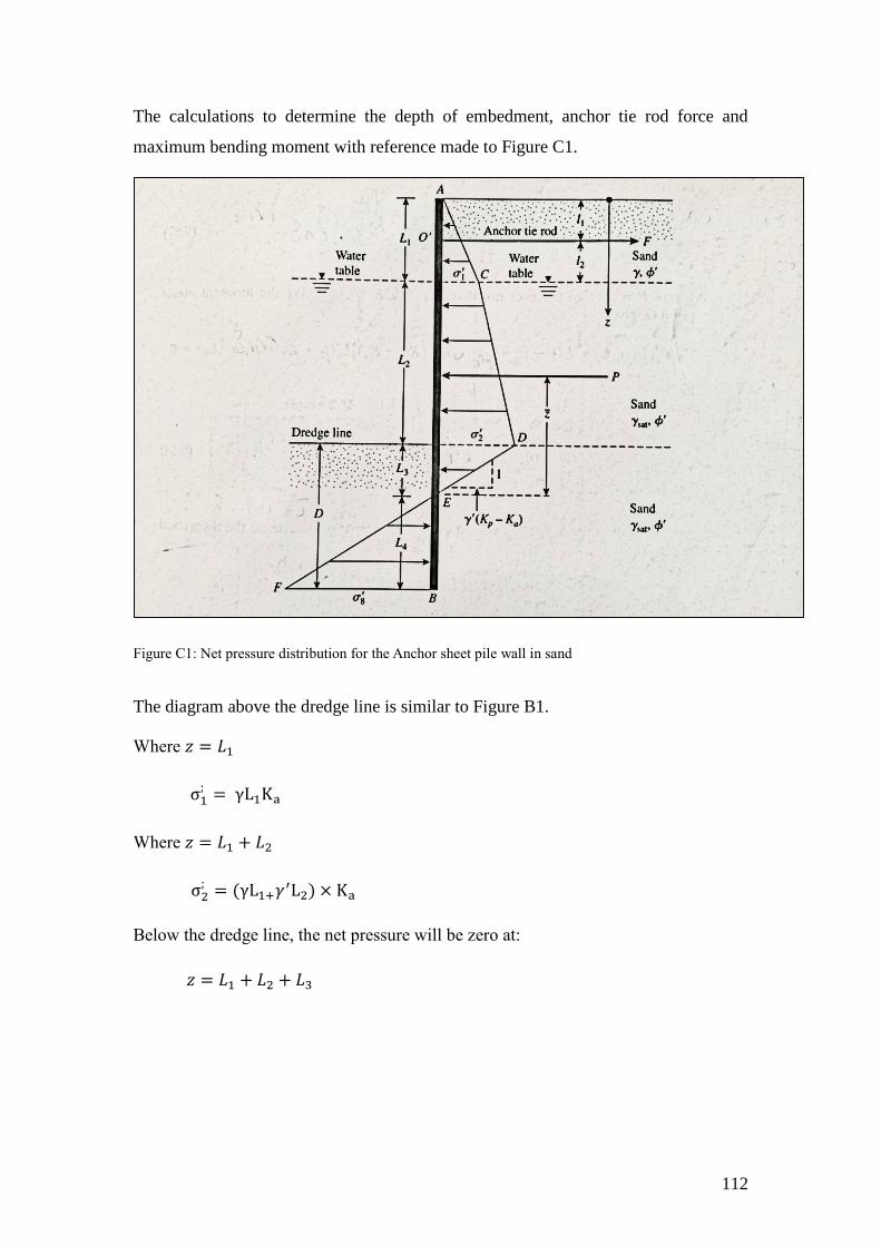
112

The calculations to determine the depth of embedment, anchor tie rod force and

maximum bending moment with reference made to Figure C1.

Figure C1: Net pressure distribution for the Anchor sheet pile wall in sand

The diagram above the dredge line is similar to Figure B1.

Where 𝑧 = 𝐿1

σ1; = γL1Ka

Where 𝑧 = 𝐿1 + 𝐿2

σ2; = (γL1+𝛾′L2) × Ka

Below the dredge line, the net pressure will be zero at:

𝑧 = 𝐿1 + 𝐿2 + 𝐿3

113

Step 1: Calculate Ka and Kp

Ka = tan2 (45 − ∅2⁄ )

= tan2(45 − 402⁄ )

= 0.217

Kp = tan2 (45 + ∅2⁄ )

= tan2(45 + 402⁄ )

= 4.598

Step 2: Calculate σ1; and σ2

;

σ1; = γL1Ka

= 18.85 × 3 × 0.217

= 12.27 KPa

σ2; = (γL1+𝛾′L2) × Ka

= [(18.85 × 3 + (20.33 − 9.81) × 6]0.217

= 25.96 KPa

Step 3: Determine L3, by using the relation given of 1 vertical to 𝛾′(𝐾𝑝 − 𝐾𝑎) in the

horizontal

L3 =σ2

;

𝛾′(𝐾𝑝 − 𝐾𝑎)⁄

L3 = 25.9610.52(4.598 − 0.217)⁄

L3 = 0.563 m

Step 4: Calculate P, by summing all the horizontal forces

P = 0.5 σ1; L1 + σ1

; L2 + 0.5(σ2; − σ1

; )L2 + 0.5σ2; L3

= (0.5 × 12.27 × 3) + (12.27 × 6) + 0.5(25.96 − 12.27)6 + (0.5 × 25.96 ×

0.604)

= (18.405) + (73.62) + 40.26 + (7.83992)

114

= 140.12 𝑘𝑁/𝑚

Step 5: Calculate z̅, i.e., the centre of the pressure for the area ACDE by taking the

moments about point E

�̅� =

⌈⌈⌈⌈⌈⌈ 0.5p1L1 ∗ (

𝐿1

3+ 𝐿2 + 𝐿3) +

p1L2 ∗ (𝐿3 +𝐿2

2) +

0.5(p2 − p1)L2 ∗ (𝐿3 +𝐿2

3) +

0.5p2L3 ∗𝐿3

3 ⌉

⌉⌉⌉⌉⌉

𝑃⁄

�̅� =

⌈⌈⌈⌈⌈⌈ (0.5 × 12.27 × 3) × (

3

3+ 6 + 0.604) +

(12.27 × 6) × (0.604 +6

2) +

0.5(25.96 − 12.27)6 × (0.604 +6

3) +

0.5 × 25.96 × 0.604 ∗0.604

3 ⌉

⌉⌉⌉⌉⌉

140.12⁄

�̅� = 3.66 𝑚

Step 6: Calculate the unknown length L4 by means of trial and error:

L34 + 1.5 × L4

2(l2 + L2 + L3) −3P[(L1+L2+L3)−(z̅+l1)]

𝛾′(𝐾𝑝−𝐾𝑎)= 0 Substitute 𝐿4 =

1.66

0.5634 + 1.5 × 1.662(1.5 + 6 + 3) −3×140.12[(3+6+0.563)−(3.66+1.5)]

10.52(4.598−0.217)= 0

𝐿4 = 1.66 m

Step 7: Obtain the theoretical depth of penetration as L3 + L4.

𝐷𝑡ℎ𝑒𝑜𝑟𝑒𝑡𝑖𝑐𝑎𝑙 = 𝐿3 + 𝐿4

𝐷𝑡ℎ𝑒𝑜𝑟𝑒𝑡𝑖𝑐𝑎𝑙 = 0.563 + 1.66

𝐷𝑡ℎ𝑒𝑜𝑟𝑒𝑡𝑖𝑐𝑎𝑙 = 2.22 𝑚

115

Step 8: Increase the theoretical depth with a factor of safety of 1.4

𝐷𝑎𝑐𝑡𝑢𝑎𝑙 = 𝐷𝑡ℎ𝑒𝑜𝑟𝑒𝑡𝑖𝑐𝑎𝑙 × 1.4

𝐷𝑎𝑐𝑡𝑢𝑎𝑙 = 2.22 × 1.4

𝐷𝑎𝑐𝑡𝑢𝑎𝑙 = 3.11 𝑚

Step 9: Determine the anchor force F, by summing all the horizontal forces,

F = P − 0.5 × [𝛾′(𝐾𝑝 − 𝐾𝑎)] × 𝐿42

F = 140.12 − 0.5 × [10.52 × (4.598 − 0.217)] × 1.662

F = 76.62 kN

Step 10: Calculate the point where maximum shear force occurs by making a cut on the

beam and summing the moments about that specific point z, it has been assumed that

this point of zero shear will occur where:

𝐿1 + 𝐿2 < z < 𝐿1

Therefore obtaining the following equation after summing the forces around the point

where the cut was made on the beam:

0.5 × σ1; L1 − 𝐹 + σ1

; (z − L1) + 0.5 × 𝐾𝑎𝛾′(z − L1)

2 Substitute 𝑧 =

6.599

0.5 × 12.27 × 3 − 76.62 + 12.27(5.77 − 3) + 0.5 × 0.217 × 10.52(5.77 − 3)2

z = 6.599 𝑚

And to make calculations simpler:

x = 6.599 − 3

x = 3.599 𝑚

116

Step 11: Determine the maximum bending moment by summing all the moments about

the point where zero shear force occurs:

Mmax = −(0.5 × σ1; L1) × [𝑥 + (

L13

⁄ )] + 𝐹(𝑥 + 1) − σ1; x × (

𝑥

2) − 0.5𝐾𝑎𝛾

′(𝑥2)𝑥

3

Mmax = −(0.5 × 12.27 × 3) × [3.599 + (3 3⁄ )] + 76.62(3.599 + 1) − 12.27 × 3.599 ×

(3.599

2) − 0.5 × 0.217 × 10.52(3.5992)

3.599

3

Mmax = 174.26 kN.m

Developing a Numerical Model for the Design of Sheet Pile ... · Developing a Numerical Model for...

Documents

Transcript of Developing a Numerical Model for the Design of Sheet Pile ... · Developing a Numerical Model for...