Developed by Dr. Jingxuan Li, Dong Yang, Charles Luzzato ...

1Jingxuan LIDepartment of Aeronautics

Open Source Combustion Instability Low Order Open Source Combustion Instability Low Order Simulator for Longitudinal ModesSimulator for Longitudinal Modes

(OSCILOS_long)User guide for version 1.4

Developed by Dr. Jingxuan Li, Dong Yang, Charles Luzzato and Dr. Aimee S. Morgans*

Published under the BSD Open Source license Programmed with MATLAB 2014a

First released on April 23, 2014Website: http://www.oscilos.com/

Contact: [email protected] and [email protected]


What is OSCILOS?What is OSCILOS? The open source combustion instability low-order simulator (OSCILOS) is an open

source code for simulating combustion instability. It is written in Matlab ®/ Simulink® and is very straightforward to run and edit.

It can simulate both longitudinal and annular combustor geometries. It represents a combustor as a network of connected modules.

The acoustic waves are modeled as either 1-D plane waves (longitudinal combustors) or 2-D plane/circumferential waves (annular combustors).

A variety of inlet and exit acoustic boundary conditions are possible, including open, closed, choked and user defined boundary conditions.

The response of the flame to acoustic waves is captured via a flame model; flame models ranging from linear n- τ models to non-linear flame describing functions, either defined analytically or loaded from experimental / CFD data, can be prescribed.

The mean flow is calculated simply by assuming 1-D flow conditions, with changes only across module interfaces or flames.

This current version is for longitudinal modes. This assumes a longitudinal/cannular/can combustor geometry, or an annular geometry but where only plane acoustic waves are known to be of interest.


Who is developing OSCILOS?Who is developing OSCILOS? OSCILOS is being developed by Dr Aimee Morgans, Dr. Jingxuan Li, Dong Yang and

co-workers in the Department of Aeronautics, Imperial College London, UK. More details about the development team are available on the website:

http://www.oscilos.com/http://www.oscilos.com/ Current team members: Dr. Aimee S. Morgans (project lead)Dr. Jingxuan LiDong YangCharles Luzzato Dr. Xingsi Han The latest version of OSCILOS is available from our Github repository: https://github.com/MorgansLab/ https://github.com/MorgansLab/ Contributions are welcome and can be submitted with GitHub pull request. These will be

reviewed and accepted by the team.


Required Matlab toolboxesRequired Matlab toolboxes

Control System Toolbox Matlab Optimization Toolbox Robust Control Toolbox Simulink Symbolic Math Toolbox


Main consoleMain console

1. Menu Bar1. Menu BarThe menu bar organizes the GUI menu hierarchy using a set of pull-down menus.A pull-down menu contains items that perform executed actions. 2. Information window2. Information windowKey information from the program run is printed in the information window.

2

1


Menu BarMenu Bar FileFile

New case Load… Save…

InitializationInitialization Chamber dimensions Thermal properties Flame model Boundary conditions

Frequency domain analysisFrequency domain analysis Eigenmode calculation

Time domain simulationTime domain simulation Examination of the Green's function Parameter configuration simulation Results output and plot

HelpHelp About User guide


New case: This menu option is used to clear current results and create a new calculation.Load...: This menu option is used to load data from existing Mat file. The current calculation results will be deleted once the user clicks Yes.Save...: This menu option is used to save the current calculation results as a Mat file.

FileFile


Initialization / Chamber dimensionsInitialization / Chamber dimensions

This menu option is used to set the geometric dimensions of the combustor.

(a) Interface for Rijke tube (b) Combustor geometry is loaded from external txt file



The length and radius of the combustor can be quickly configured for the case of a Rijke tube. For complicated combustor geometries, users can load the information from an external txt file by

clicking load. It is better to create the txt file as the form of CD_example.txt in the subProgram folder. The format of data is shown in the following table:

where, x means axial position of each sectional interface; r indicates the radius of each section; Interface index represents the type of interface between modules: '0': a simple area change; '10': with heat addition and without heat perturbation; '11': with heat perturbations. Module index indicates the type of tube between this and the following interface: '0': straight constant area duct; '1': duct with linearly changing radius. The schematic of the combustor can be previewed by clicking Plot.The current configuration is saved by clicking OK. The key information will be printed in the information window.



OSCILOS can account for cases of multiple heat sources (multi-flames), by setting the section indices to '10' or '11' for the desired interfaces. The following figure shows the schematic view of an example with two flames, in which the red lines are used to represent the unsteady heat sources (flames).



OSCILOS can account for geometry modules whose sectional radius gradually changes with axial location.

For example, the following table shows the combustor dimensions of the key interfaces. The module index at interface 2 is “1”, meaning that the radius of the section between interfaces 2 and 3 changes linearly with axial position.

This kind of module is split into equally spaced segments for numerical treatment. The number of splits or segments can be set in a jumped window as shown in the top right figure.

The schematic view of the above combustor is shown in the bottom right figure.


InitializationInitialization // PassivePassive damper(s) damper(s)

• Helmholtz resonators (HRs) and perforated liners can be added to the combustor system by choosing to use passive damper(s) after setting up the combustor dimensions.

• For the “ Damper type ” , if the “ Helmholtz resonator ” is chosen, users need to• set its “ Location ” , “ Neck length ”,

“Neck area” , “Cavity volume” and “Cavity Temperature”,

• choose either a “ Linear ” or “Nonlinear” HR model. • If “Linear” is chosen, a “Mean

hole Mach no. ” for the neck should be given,

• If “ Nonlinear ” is chosen, the “ Discharge coefficient ” must be set.


• If “Perforated liner” is chosen for the “Damper type”, users need to

• set its “ Start location ” , “ Length ” and “Liner temperature”,

• If “Single Liner” is chosen, four parameters ( “ Hole radius ”, “ Hole distance ” , “ Hole mean Mach no. ” and “ Thickness ”) need to be set,

• If “ Double liner ” is chosen, another four parameters (“Hole radius ” , “ Hole distance ”, “Layer radius” and “Thickness” for the second perforated layer) need also to be set.

• choose either a “ Single liner ” or “Double liner” type,

• choose either a “ Large cavity ” or “Rigid wall” outside boundary type for the outer liner. “ Wall radius ” should be set if the “Rigid wall ” is chosen.

InitializationInitialization // PassivePassive damper(s) damper(s)


Initialization / Thermal propertiesInitialization / Thermal properties

This menu is used to set the inlet mean flow properties and the mean heat addition.

2

1

3

1. Plot panel1. Plot panelThis panel is used to plot the distribution of mean velocity and mean temperature with axial position.2. Mean flow properties panel 2. Mean flow properties panel The inlet mean pressure, temperature and flow velocity/Mach number are set in this panel.3. Mean heat addition panel3. Mean heat addition panelThis panel is used to configure the heat addition, once there is (are) heat source(s) inside the combustor.


Initialization / Thermal propertiesInitialization / Thermal properties The mean flow and thermal properties within each combustor module are considered uniform for constant

sectional area modules.

Modules with varying sectional radius are split into equally spaced segments for numerical treatment. The mean flow and thermal properties are considered uniform in each segment.

Users can choose a model for the (mean) heat addition from the drop-down menu.

Heat from a heating grid (Tb/Tu is given), where Tu represents the temperature upstream of the grid, and Tb downstream of the grid. This is often used in the case of a Rijke tube.

Heat from fuel combustion.

1. Users can choose the fuel from the pop-up menu, including CH4, C2H4, C2H6, C3H8, C4H8, C4H10 (n-butane), C4H10 (isobutane) and C12H23 (Jet-A).

2. Users can also set: (a)Equivalence ratio

(b)Combustion efficiency

(c) Dilution ratio, which is used when a bias flow is accounted for.

The mean properties in different modules can be calculated by clicking "Calculate" once all the inputs have been completed.

For multiple flames cases, users need to set the parameters for each heat source. The corresponding heat release rate for each heat source is shown in the text box after calculation.

The distribution of mean temperature and mean flow velocity can be previewed by clicking "Plot figure".

The current configuration is saved by clicking "OK". The key information will be printed in the information window.


Initialization / Flame modelInitialization / Flame model This panel is used to choose (flame) model for each unsteady heat source.

The (flame) model describes how the (normalized) unsteady heat release rate of the unsteady heat source (flame) responds to (normalized) velocity fluctuations.

Four choices can be prescribed: A linear (flame) transfer function model; A simple nonlinear (flame) describing function model,

which is assumed can be decoupled as a nonlinear saturation model and a linear (flame) transfer function (FTF) model. Experimental/CFD (flame) transfer functions (loaded

from an external mat file) for different velocity perturbations upstream of the flame. The FTF data are fitted within OSCILOS with state-space models. The fully non-linear G-Equation model (Williams

1988). When users choose a heat source and a (flame) model from the drop pop-up menus and click

Edit, a corresponding window appears for detailed configuration. The button OK will be enable once the flame models for all unsteady heat sources have been

configured.


Initialization / Flame model / Linear FTFInitialization / Flame model / Linear FTFThis panel appears once users choose linear FTF model.

1

2

1. Parameters configuration panel1. Parameters configuration panelThis panel is used to configure the parameters of the flame model. Users can choose the linear FTF from the drop-down menu. The left figure shows the n-tau model configuration panel. Panels corresponding to the other 3 choices are shown in the 3 bottom figures. 2. Plot panel2. Plot panelThe evolutions of gain and phase lag of the FTF with frequency are plotted once users click Plot figure.

(a) 1st order low pass filter model (b) 2nd order low pass filter model (c) polynomial transfer function


Flame transfer functionFlame transfer function


Initialization / Flame model /Nonlinear FDF model (1)Initialization / Flame model /Nonlinear FDF model (1)

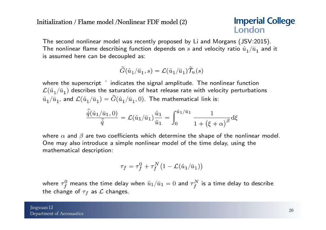
Two kinds of nonlinear flame describing functions can be prescribed. The first is an abrupt heat release rate ratio saturation model proposed by Dowling (JFM:1997), which can be mathematically expressed as:

Where α is a constant associated with the saturation (0≤α≤1) and denotes the heat release rate ratio for weak perturbations, which can be calculated from the linear flame transfer function.


Initialization / Flame model /Nonlinear FDF model (2)Initialization / Flame model /Nonlinear FDF model (2)


Initialization / Flame model /Nonlinear FDF modelInitialization / Flame model /Nonlinear FDF model

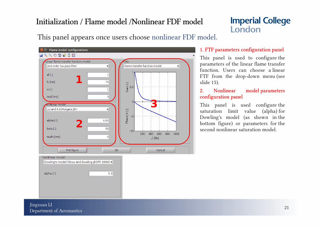
This panel appears once users choose nonlinear FDF model.

1

23

1. FTF parameters configuration panel1. FTF parameters configuration panelThis panel is used to configure the parameters of the linear flame transfer function. Users can choose a linear FTF from the drop-down menu (see slide 15). 2. Nonlinear model parameters 2. Nonlinear model parameters configuration panelconfiguration panelThis panel is used configure the saturation limit value (alpha) for Dowling's model (as shown in the bottom figure) or parameters for the second nonlinear saturation model.


Initialization / Flame model /Nonlinear FDF modelInitialization / Flame model /Nonlinear FDF model3. Plot panel3. Plot panelThree kinds of plots can be prescribed:(1) Flame transfer function(2) Nonlinear saturation model(3) Flame describing function

(a) Flame transfer function (b) Nonlinear saturation model (c) Flame describing function


Initialization /Initialization /Flame model /Loaded and Flame model /Loaded and fitted FDF from experiment or CFD datafitted FDF from experiment or CFD data

This panel appears once users choose Experimental/CFD fitted FDF.

1 2

1. FDF editing panel 1. FDF editing panel Users can add, edit or remove the flame transfer functions for different flame velocity perturbation levels obtained from experiment or CFD simulation. 2. Plot panel2. Plot panelThe original data and fitted FDF can be viewed from this plot.


Initialization /Initialization /Flame model /Loaded and Flame model /Loaded and fitted FDF from experiment or CFD datafitted FDF from experiment or CFD data

Once the button Add FTF for a new velocity ratio is clicked, a window for displaying the experimental/CFD FTF and fitting will appear.

1. Data import panel 1. Data import panel Users can set the velocity ratio and then import

experimental/CFD FTF from an external Mat file. (It is better to save the data in a Mat file prior to running OSCILOS. The data format is for example shown in the right bottom figure).

2. Fitting parameters configuration panel 2. Fitting parameters configuration panel Users need to set the fitting frequency range, time

delay correction, fitting order and relative degree of denominator compared to numerator, which are used for fitting, via the Matlab command “fitfrd”.

3. Plot panel3. Plot panelThe original data (markers) and fitted FTF (solid

line) can be viewed from this plot. The fitting process is operated upon clicking Fit

and plot. The original FTF data and fitting parameters are

saved by clicking save fitting.

1

32

The first column is the frequency and the second one is the corresponding gain or phase lag (in rad).


Initialization / Flame model / G-EQuationInitialization / Flame model / G-EQuationThis panel appears once users choose the G-Equation model.

1. Flame properties panel1. Flame properties panelThis panel is used to set the flame properties for the G-Equation. The user can set the laminar flame velocity (which should be smaller than incoming mean flow), the number of points used to discretize the flame, the flame holder radius and the flame time delay factor.2. Steady flame shapes panel2. Steady flame shapes panelWhen the user clicks Plot figure, the steady flame shape and the flame holder are plotted for the selected heat source location.


Initialization/Boundary conditionsInitialization/Boundary conditions

This menu is used to set the inlet and outlet boundary conditions. Six kinds of boundary conditions are provided: Open end (R = -1). Closed end (R = 1). Choked end. User defined (Amplitude and time delay)... User defined (Amplitude and phase)... User-defined model using a polynomial transfer function by inputting the numerator coefficients b and denominator coefficients a. The order of the numerator should not be larger than that of denominator n ≤ m.


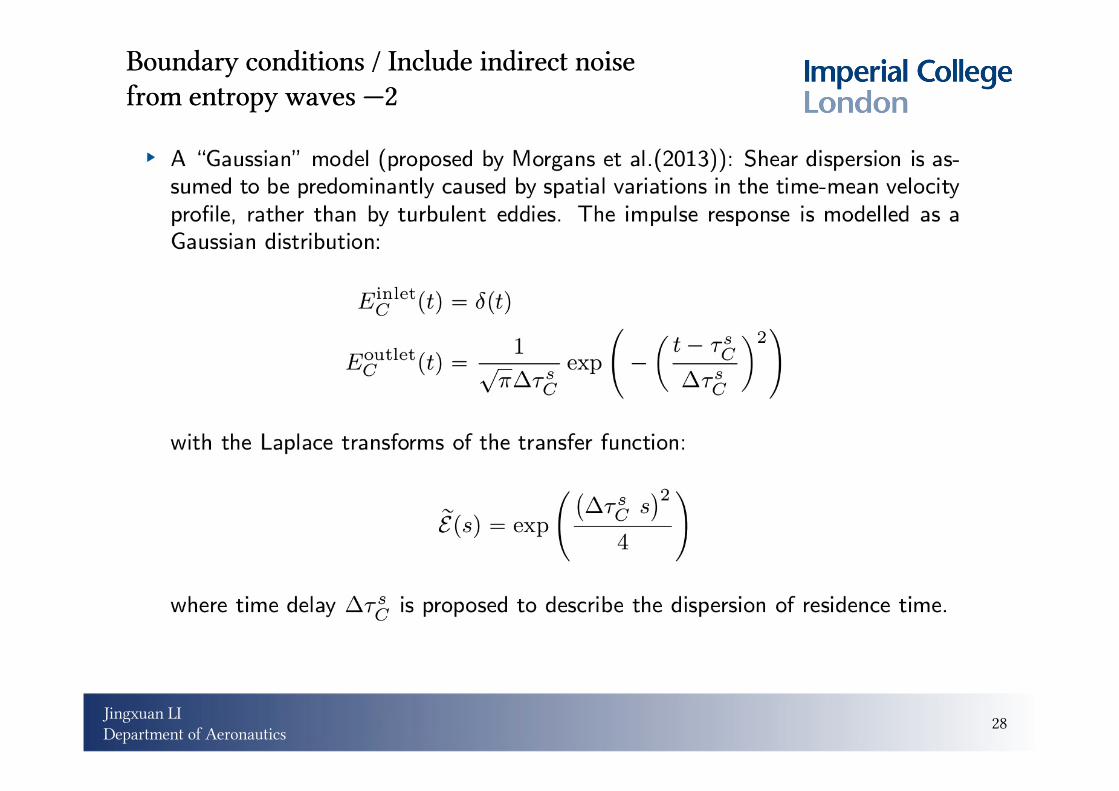
Boundary conditions / Include indirect noiseBoundary conditions / Include indirect noisefrom entropy waves from entropy waves ——11


Boundary conditions / Include indirect noiseBoundary conditions / Include indirect noisefrom entropy waves from entropy waves ——22


Freq. domain analysis / Eigenmode calculationFreq. domain analysis / Eigenmode calculation

Once all initializations are complete, the user can then progress to the “Eigenmode calculation” panel.

1

23



1. Velocity ratios and eigenmode scan domain configuration panel1. Velocity ratios and eigenmode scan domain configuration panel

Users need to set the minimum and maximum velocity ratios before the flame if the nonlinear flame describing function model has been chosen (as shown in first figure). The number of velocity ratio samples is also needed to equally space the velocity ratio range.

In the case that the flame describing function was provided by experimental or CFD data, these “edit” boxes are not enabled -- their values are automatically assigned (as shown in second figure).

In the case that linear flame transfer function model was chosen or there is no flame or unsteady heat source inside the combustor, the “edit” boxes are not visible (as shown in the third figure).

Users need to define a scan range (including frequency and growth rate) to search for eigenvalues within this range, as shown in the right bottom figure. This can be done by clicking “Set scan range”.

When all the setting has been completed, users can calculate the eigenvalues for a set of velocity ratios (or an arbitrary velocity ratio for linear FTF or no flame case).



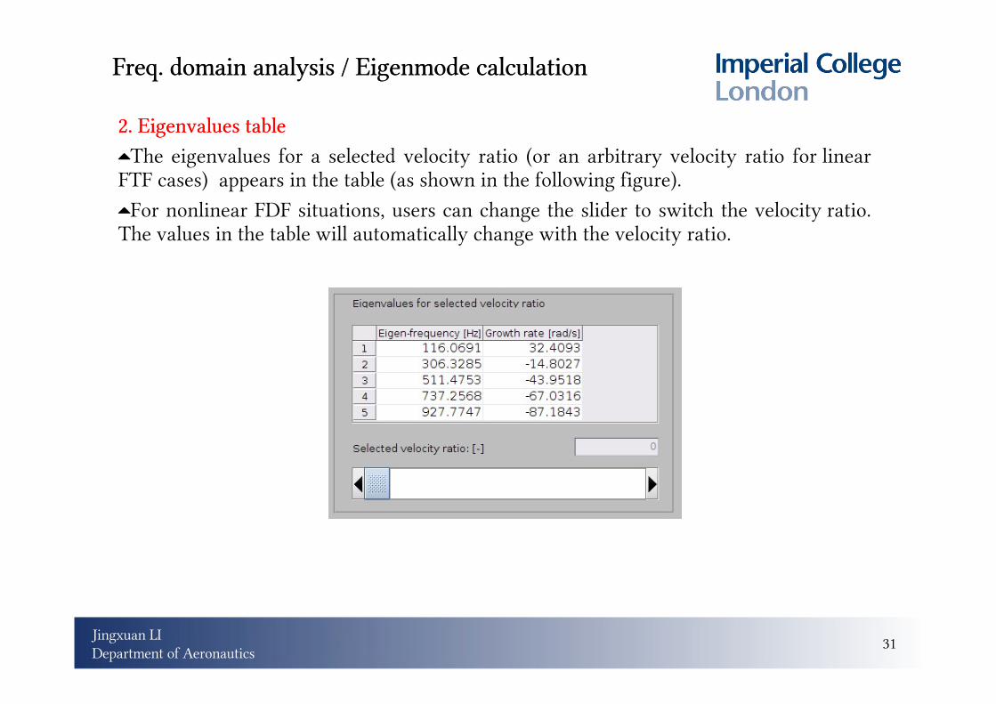
2. Eigenvalues table 2. Eigenvalues table The eigenvalues for a selected velocity ratio (or an arbitrary velocity ratio for linear FTF cases) appears in the table (as shown in the following figure).For nonlinear FDF situations, users can change the slider to switch the velocity ratio. The values in the table will automatically change with the velocity ratio.



3. Plot panel3. Plot panel Users can plot three kinds of figures from the choices of the pop-up menu:1.A contour map showing the eigenvalue locations (growth rate and frequency).2.The mode shape (velocity perturbation amplitude (top figure) and pressure disturbance amplitude (bottom figure) distributions along the axial position).3.The evolution of growth rate (top figure) and eigen-frequency (bottom figure) with increasing velocity ratio for a selected mode. This plot is not available for linear FTF cases.

(a) contour map (b) mode shape (c) evolution of eigenvalues


Time domain simulation /Time domain simulation /Examination of the Green's functionExamination of the Green's function

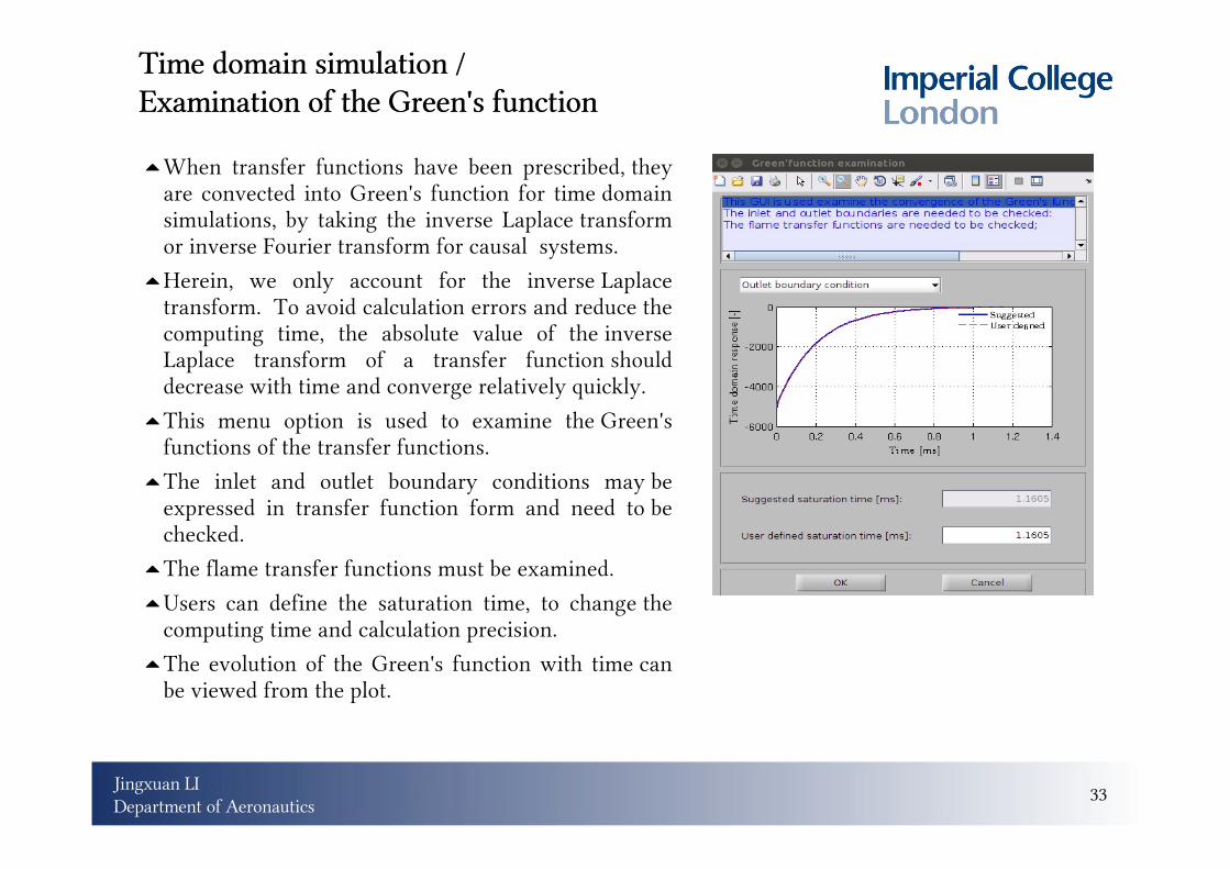
When transfer functions have been prescribed, they are convected into Green's function for time domain simulations, by taking the inverse Laplace transform or inverse Fourier transform for causal systems.

Herein, we only account for the inverse Laplace transform. To avoid calculation errors and reduce the computing time, the absolute value of the inverse Laplace transform of a transfer function should decrease with time and converge relatively quickly.

This menu option is used to examine the Green's functions of the transfer functions.

The inlet and outlet boundary conditions may be expressed in transfer function form and need to be checked.

The flame transfer functions must be examined.Users can define the saturation time, to change the

computing time and calculation precision. The evolution of the Green's function with time can

be viewed from the plot.


Time domain simulation /Time domain simulation /Parameters configurationParameters configuration

1

2

3

4

1. Simulation time and time step1. Simulation time and time stepThis panel is used to configure the simulation stop time and time step. The minimum time delay is provided and the time step should be smaller than this value. 2. Simulation samples per loop2. Simulation samples per loopFor linear or weakly nonlinear system, the computing speed can be accelerated by increasing the number of time steps in one calculation loop. The maximum number of steps per loop is provided and users can define the number of time steps per loop in the text box. If this box is not active, that means the computing cannot be accelerated and the default value is 1. 3. Velocity ratio upper limit3. Velocity ratio upper limitTo avoid signals increasing towards infinity for unstable systems, users need to define an upper limit. 4. Background noise4. Background noiseThe background noise information can be defined in this panel. These noises can be used to stimulate any instabilities within the combustor.


Time domain simulation /Simulation...Time domain simulation /Simulation...

Once all initializations are complete, the user can then progress to the “simulation...” panel.

For linear systems or nonlinear systems with an abrupt saturation limit (Dowling's model), the calculation is simpler and a wait-bar box appears to show the computing progress.

The calculation becomes more complicated when users

have chosen flame describing function models (such as our model). The transfer function changes with velocity ratio and the Green's function should be updated every time step based on the velocity ratio at the corresponding time step. However, calculating the velocity ratio needs knowledge of the Green's function.

The calculation method can then be summarized using the flow chart on the right.


Time domain simulation /Simulation...Time domain simulation /Simulation...

When users have chosen a flame describing function model (such as our model), a calculation monitor window, as shown in the right figure, appears to show the calculation progress.

The evolution of velocity ratio before the flame is plotted in the figure.

The calculation error is also shown.


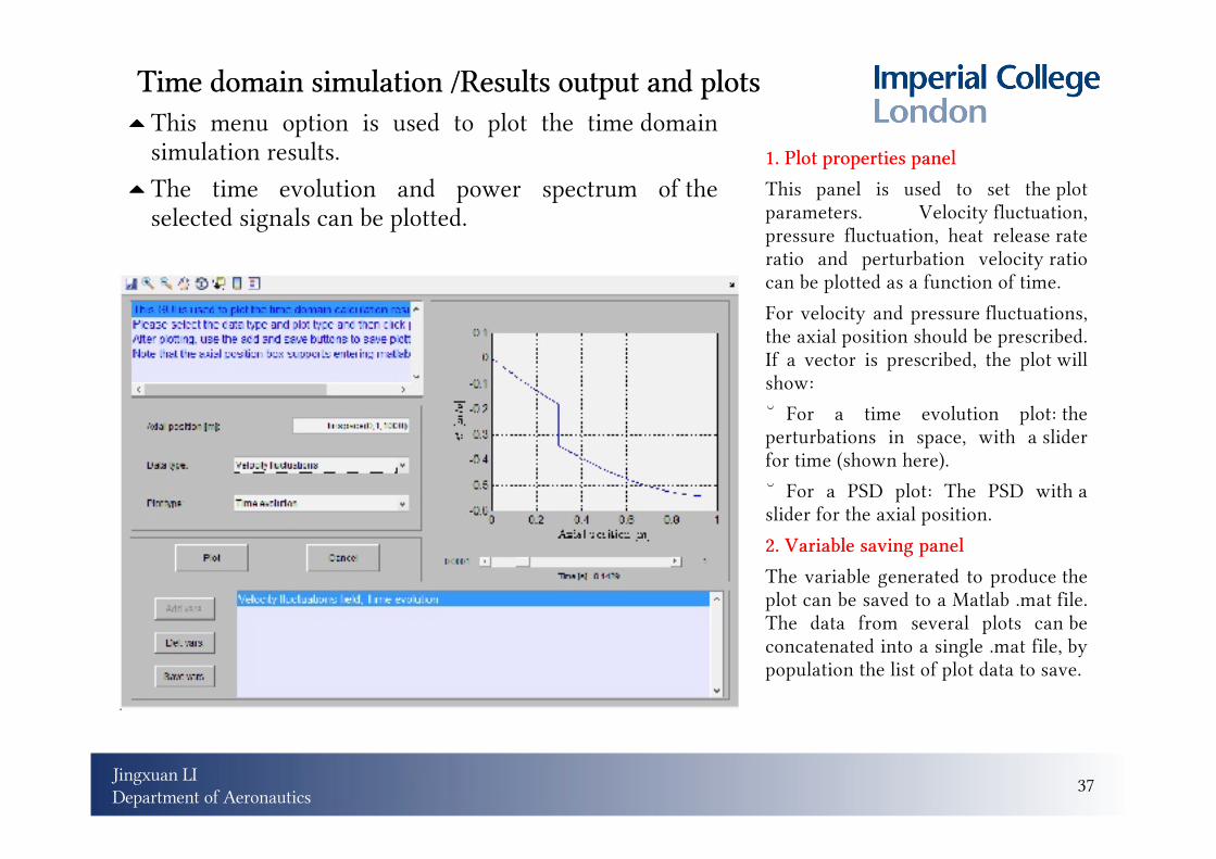
Time domain simulation /Results output and plotsTime domain simulation /Results output and plots This menu option is used to plot the time domain

simulation results. The time evolution and power spectrum of the

selected signals can be plotted.

1. Plot properties panel1. Plot properties panelThis panel is used to set the plot parameters. Velocity fluctuation, pressure fluctuation, heat release rate ratio and perturbation velocity ratio can be plotted as a function of time. For velocity and pressure fluctuations, the axial position should be prescribed. If a vector is prescribed, the plot will show: For a time evolution plot: the perturbations in space, with a slider for time (shown here). For a PSD plot: The PSD with a slider for the axial position.2. Variable saving panel2. Variable saving panelThe variable generated to produce the plot can be saved to a Matlab .mat file. The data from several plots can be concatenated into a single .mat file, by population the list of plot data to save.


Time domain simulation /Results output and plotsTime domain simulation /Results output and plots

This menu option is used to plot the time domain simulation results. The time evolution and power spectrum of the selected signals can be plotted.


Example 1 Example 1 A cold open tubeA cold open tube

Users can directly load the file “Case_A_cold_open_tube.mat” from the “cases” folder to see the detailed configuration and results.

1. Combustor dimensions1. Combustor dimensionsThe combustor type is set to Rijke tube.The dimensions are shown in the right figure.There is no heat addition in the tube.

2. Mean flow and thermal properties configuration2. Mean flow and thermal properties configurationSince there is no heat addition, the panel for heat addition configuration is not visible. The mean flow properties at the inlet are shown in the following figure.

3. Boundary conditions3. Boundary conditionsSince there is no heat perturbation, the user directly progresses to the boundary conditions configuration panel. The inlet and outlet are set to open and the pressure reflection coefficients are set to negative constant values, as shown in the right figures.



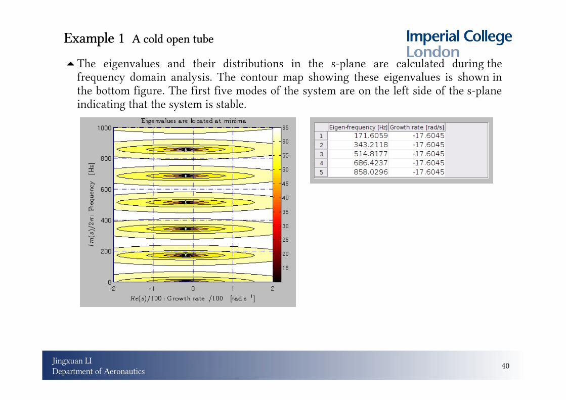
The eigenvalues and their distributions in the s-plane are calculated during the frequency domain analysis. The contour map showing these eigenvalues is shown in the bottom figure. The first five modes of the system are on the left side of the s-plane indicating that the system is stable.



We now progress to time domain simulations. The background noise configuration is shown in the following figure.

The white noise has a power of 10 dB and stops at t = 0.5 s.

The time evolution and power spectrum of the pressure perturbations at the axial position x = 0.6 m are shown in the following figures. In the presence of additional white noise, all of the excited modes are stable and disturbances are attenuated. As shown in the PSD figure, the frequencies of the peaks are the same as those predicted with the frequency domain analysis.

(a) time evolution (b) PSD


Users can directly load the file “Case_Hot_tube.mat” from the “cases” folder to see the detailed configuration and results.

1. Combustor dimensions1. Combustor dimensionsThe combustor type is set to Rijke tube.The dimensions are shown in the right figure.

2. Mean flow and thermal properties configuration2. Mean flow and thermal properties configurationThe mean flow properties at the inlet are shown in the following figure. Heat is from a heat grid and the temperature ratio is set to 2. The mean heat release rate is calculated as 9.7201 kW.

Example 2 Hot combustorExample 2 Hot combustor



4. Boundary conditions4. Boundary conditionsThe inlet is set to closed and the outlet is set to open. The reflection coefficient is expressed as a transfer function as shown in the bottom figure.

3. Flame model3. Flame modelOur nonlinear flame describing function is chosen as the flame model.The parameters configuration for the flame transfer function and the nonlinear saturation model are shown in the right figure.



The right figure shows the evolution of growth rate and resonant frequency of the first mode with velocity ratio before the flame. With increasing normalized velocity perturbations, the growth rate decreases and a limit cycle is finally established when the velocity ratio equals to 0.3.

This has been validated in the time domain simulation results. The figures at the bottom show the evolution of velocity ratio with time.


Example 3: A laboratory combustor rigExample 3: A laboratory combustor rig The experiments were carried out by Palies and co-workers in

Laboratory EM2C. The combustor includes a plenum, an injection unit and a combustion chamber terminated by an open end. The compact flame is stabilized at the beginning of the combustion chamber.

OSCILOS can account for this complicated combustor shape and the combustor shape can be viewed from the following figure.

Experiments were carried out with the plenum and chamber comprising varying lengths to change the eigenvalues of the combustor. Herein, we only take one unstable case for the comparison between the calculation results from OSCILOS and the experimental results.


Example 3: A laboratory combustor rigExample 3: A laboratory combustor rig

Mean flow and thermal properties: methane is used as the fuel and the equivalence ratio is 0.7. The measured mean temperature of the burned gases is 1600 K. So that the calculated mean temperature matches the experimental result, the combustion efficiency is set equal to 0.825.

Flame model: the experimental flame describing functions (markers) and their fitted results (solid lines) are shown in the right figure.

Boundary conditions: the inlet boundary condition is set to closed with a reflection coefficient of 0.96, and the outlet is set to open.


Example 3: a laboratory combustor rig Example 3: a laboratory combustor rig

The distribution of eigenvalues are shown in the following contour maps for two velocity ratios. The main unstable modes are highlighted by the white stars.

With increasing flow velocity, the growth rate of the unstable mode decreases to zero and a limit cycle is established. The predicted resonant frequency and velocity ratio before the flame when the limit cycle is established are 126 Hz and 0.683, respectively. In the experiment, the resonant frequency and velocity ratio before the flame when the limit cycle is established are 126 Hz and 0.68, respectively.

The prediction matches well the experimental results.

Developed by Dr. Jingxuan Li, Dong Yang, Charles Luzzato ...

Documents

Transcript of Developed by Dr. Jingxuan Li, Dong Yang, Charles Luzzato ...