Develop and Implement a Freeze Thaw Model Based Seasonal ...
140
Develop and Implement a Freeze Thaw Model Based Seasonal Load Restriction Decision Support Tool Final Report Report Number: OR16-009 Michigan Department of Transportation Office of Research Administration 8885 Ricks Road Lansing, MI 48909 By Zhen (Leo) Liu, Ting Bao, Michael Billmire, Stanley Vitton, John Bland, and Min Wang Michigan Technological University 1400 Townsend Drive Houghton, MI 49931 August 2019
Transcript of Develop and Implement a Freeze Thaw Model Based Seasonal ...

Develop and Implement a Freeze Thaw Model Based Seasonal Load
Restriction Decision Support Tool
Final Report
Report Number: OR16-009
Michigan Department of Transportation
Office of Research Administration
8885 Ricks Road
Lansing, MI 48909
By
Zhen (Leo) Liu, Ting Bao, Michael Billmire, Stanley Vitton, John Bland, and Min Wang
Michigan Technological University
1400 Townsend Drive
Houghton, MI 49931
August 2019

ii
Technical Report Documentation Page
1. Report No.
OR16-009 2. Government Accession No.
N/A 3. MDOT Project Manager
Melissa Longworth
4. Title and Subtitle
Develop and Implement a Freeze Thaw Model Based Seasonal Load
Restriction Decision Support Tool
5. Report Date
August 2019
6. Performing Organization Code
N/A
7. Author(s)
Zhen (Leo) Liu, Stanley Vitton, Michael Billmire, and Min Wang
8. Performing Org. Report No.
N/A
9. Performing Organization Name and Address
Michigan Technological University
1400 Townsend Drive
Houghton, MI 49931
10. Work Unit No. (TRAIS)
N/A
11. Contract No.
2016-0067
11(a). Authorization No.
Z9
12. Sponsoring Agency Name and Address
Michigan Department of Transportation Research Administration
8885 Ricks Rd.
P.O. Box 30049
Lansing MI 48909
13. Type of Report & Period Covered
Final Report
5/01/2017 to
3/1/2020 14. Sponsoring Agency Code
N/A
15. Supplementary Notes
16. Abstract
This report summaries a study on the development and implementation of a freeze thaw model based
Seasonal Load Restriction (SLR) decision support tool. A multivariable prediction approach for freezing and
thawing depths were proposed. The approach was implemented with input from weather data and Road
Weather Information System (RWIS) data, leading to statistical models for site-specific predictions.
Predictions made with the approach were validated against freezing and thawing depths calculated with
subsurface temperatures measured by temperature sensors at the MDOT RWIS sites. A detailed procedure
was proposed for predicting the start and end dates of the SLR policy, and this procedure was evaluated and
validated with frost tube measurements and recorded SLR dates. The above freezing and thawing depth
predictions and SLR date predictions were automated in a web-based app, i.e., www.mdotslr.org, which is
available to the public. For app, weather and RWIS data starting from 2013 and Geographic Information
System (GIS) data covering Michigan were imported and managed as local databases on the backend server.
In addition, daily weather and RWIS data including weather 5-day forecast were imported via APIs in real
time for real-time for predictions of freezing and thawing depths and SLR dates. The app provides functions
for predicting and visualizing temperature, freezing/thawing indices, degree of SLR, and SLR dates in terms
of curves and contour maps. Maximum freezing depth contours can also be generated for any given period
of time for pavement design and other purposes. All the data is available via the data portal of the app and
can be downloaded. The study provides high-accuracy methods for predicting freezing and thawing depths
and SLR dates and a convenient web-based tool for road engineers and users.
17. Key Words
Freeze-Thaw, Spring Load Restriction, Freezing Index,
Frost Depth, Thawing Index, Thawing Depth, Road Weather
Information System, Web-Based App
18. Distribution Statement
No restrictions. This document is available to
the public through the Michigan Department
of Transportation.
19. Security Classification - report
Unclassified 20. Security Classification - page
Unclassified 21. No. of Pages 22. Price
N/A

iii

iv
Acknowledgment
The authors like to thank the Michigan Department of Transportation (MDOT) for the financial
support and the MDOT staff for their cooperation and for offering training, data, access to MDSS,
feedback on preliminary results. In addition, the authors gratefully acknowledge the Minnesota
Department of Transportation (MNDOT) for providing the MnROAD and SLR data and for its
assistance. The authors want to extend their appreciation to the Transportation Research Board
technical committee AFP50 Seasonal and Climatic Effects on Transportation Infrastructure for
the feedback and technical support.
Research Report Disclaimer
“This publication is disseminated in the interest of information exchange. The Michigan
Department of Transportation (hereinafter referred to as MDOT) expressly disclaims any
liability, of any kind, or for any reason, that might otherwise arise out of any use of this
publication or the information or data provided in the publication. MDOT further disclaims any
responsibility for typographical errors or accuracy of the information provided or contained
within this information. MDOT makes no warranties or representations whatsoever regarding
the quality, content, completeness, suitability, adequacy, sequence, accuracy or timeliness of the
information and data provided, or that the contents represent standards, specifications, or
regulations.”
App Disclaimer
“This website is a prototype application under development to evaluate various seasonal load
restriction models for Michigan roadways. It is a product of an ongoing joint research project
between the Michigan Department of Transportation (MDOT) and Michigan Technological
University. This is an evolving prototype and is not used for the placement and removal of seasonal
load restrictions.”

v
Executive Summary
This report summaries a study on the development and implementation of a freeze thaw model
based Seasonal Load Restriction (SLR) decision support tool. A multivariable prediction
approach for freezing and thawing depths were proposed. The approach was implemented with
input from weather data and Road Weather Information System (RWIS) data, leading to statistical
models for site-specific predictions. Predictions made with the approach were validated against
freezing and thawing depths calculated with subsurface temperatures measured by temperature
sensors at the MDOT RWIS sites. A detailed procedure was proposed for predicting the start and
end dates of the SLR policy, and this procedure was evaluated and validated with frost tube
measurements and recorded SLR dates. The above freezing and thawing depth predictions and
SLR date predictions were automated in a web-based app, i.e., www.mdotslr.org, which is
available to the public. For app, weather and RWIS data starting from 2013 and Geographic
Information System (GIS) data covering Michigan were imported and managed as local databases
on the backend server. In addition, daily weather and RWIS data including weather 5-day forecast
were imported via APIs in real time for real-time for predictions of freezing and thawing depths
and SLR dates. The app provides functions for predicting and visualizing temperature,
freezing/thawing indices, degree of SLR, and SLR dates in terms of curves and contour maps.
Maximum freezing depth contours can also be generated for any given period of time for
pavement design and other purposes. All the data is available via the data portal of the app and
can be downloaded. The study provides high-accuracy methods for predicting freezing and
thawing depths and SLR dates and a convenient web-based tool for road engineers and users.

vi
Table of Contents
Technical Report Documentation Page ......................................................................................... ii
Acknowledgment.................................................................................................................................. iv
Research Report Disclaimer............................................................................................................. iv
App Disclaimer ...................................................................................................................................... iv
Executive Summary ............................................................................................................................... v
List of Figures ........................................................................................................................................ ix
List of Tables ........................................................................................................................................ xiii
Chapter 1 Introduction .................................................................................................................... 14
1.1 Statement of the Problem .............................................................................................. 14
1.2 Objectives of the Study ................................................................................................. 16
1.3 Research Plan ................................................................................................................ 17
1.4 Organization of This Report ......................................................................................... 21
Chapter 2 Literature Review .......................................................................................................... 25
2.1 Overview of SLR Practice ............................................................................................ 25
2.2 Relationship between SLR Practice and Freezing/Thawing ......................................... 28
2.3 Prediction of Freezing and Thawing Depths ................................................................ 31
2.4 Popular SLR Procedures based on Simple Weather Data ............................................ 34
2.4.1 FHWA-WSDOT ....................................................................................................... 34
2.4.2 MnDOT ..................................................................................................................... 35
2.4.3 MIT ........................................................................................................................... 37
2.4.4 SDDOT ..................................................................................................................... 38
2.4.5 USDA/FS-NHDOT ................................................................................................... 39
Chapter 3 Acquisition, Processing, and Evaluation of Data ................................................ 42
3.1 Data Acquisition ........................................................................................................... 42
3.1.1 Weather Data ............................................................................................................ 42
3.1.2 Acquisition of RWIS Data ........................................................................................ 44
3.1.3 Integration of GIS and Soil Data .............................................................................. 46
3.2 Data Processing ............................................................................................................. 49
3.2.1 Air and Pavement Surface Temperatures ................................................................. 49

vii
3.2.2 Subsurface Temperatures .......................................................................................... 51
3.2.3 Freezing and Thawing Depths .................................................................................. 52
3.2.4 Freezing and Thawing Indices .................................................................................. 55
3.3 Data Evaluation ............................................................................................................. 58
3.3.1 Issues in the RWIS Data ........................................................................................... 58
3.3.2 Data Mapping (vRWIS) for Site-Specific Predictions.............................................. 60
3.3.3 Data Selection via Correlation Analysis ................................................................... 61
Chapter 4 Multivariate Freezing-Thawing Depth Prediction Model ............................... 64
4.1 Overview ....................................................................................................................... 64
4.2 Field Measurements ...................................................................................................... 64
4.3 A New Freezing-Thawing Depth Prediction Model ..................................................... 66
4.4 Prediction and Evaluation of Freezing-Thawing Depth Model .................................... 70
4.5 Discussions ................................................................................................................... 76
4.5.1 Calculations of FI and TI via Surface Temperature Rather than Air Temperature .. 76
4.5.2 Prediction Improvement............................................................................................ 78
4.6 Conclusions ................................................................................................................... 80
Chapter 5 Freezing-Thawing Depth Prediction with Constrained Optimization for
Applications of Spring Load Restriction ..................................................................................... 81
5.1 Overview ....................................................................................................................... 81
5.2 Introduction ................................................................................................................... 81
5.3 Theory and Method ....................................................................................................... 83
5.3.1 Field Measurements and SLR Determination Method ............................................. 83
5.3.2 Freeze-Thaw Depth Prediction Model with Constrained Optimization ................... 86
5.4 Results ........................................................................................................................... 89
5.4.1 Site Measurements .................................................................................................... 89
5.4.2 Application of Constrained Optimization for FD/TD Predictions ............................ 94
5.5 Discussions ................................................................................................................... 98
5.5.1 Advantages of Using Constrained Optimization for FD/TD Predictions ................. 98
5.5.2 Feasibility of Using Year Cycle 1 Fitting Constants to Predict Year Cycle 2 FD/TD
99

viii
5.5.3 FD/TD Prediction Models are Better than a TI/FI Ratio for SLR Decision-Making
100
5.6 Conclusions ................................................................................................................. 102
Chapter 6 Development of Web-Based Spring Load Restriction Decision Support Tool
104
6.1 Abstract ....................................................................................................................... 104
6.2 Goals for the App Development ................................................................................. 105
6.2.1 Objectives ............................................................................................................... 105
6.2.2 Features and Benefits .............................................................................................. 105
6.3 Models and Data ......................................................................................................... 107
6.3.1 Models..................................................................................................................... 107
6.3.2 Composite Data Mapping Service .......................................................................... 109
6.3.3 Optimization of MongoDB Queries........................................................................ 110
6.4 Functions and Organization of the APP...................................................................... 110
6.5 Construction of the App .............................................................................................. 115
6.5.1 Data Transfer and Workflow .................................................................................. 115
6.5.2 Development of the Web-Based App ..................................................................... 116
6.5.3 Freezing/Thawing Index Acquisition on Backend ................................................. 117
6.5.4 Freezing/Thawing Depth Acquisition on Backend ................................................. 119
6.5.5 Refactoring .............................................................................................................. 122
6.5.6 Map Binary Search ................................................................................................. 124
6.6 Conclusions ................................................................................................................. 126
References .......................................................................................................................................... 135

ix
List of Figures
Figure 1.1 Major components of the planned research product.................................................... 22
Figure 2.1 SLR practices in the U.S. and Canada ......................................................................... 26
Figure 2.2 SLR decisions based on freezing/thawing depth predictions (modified after (Baïz et al.
2008)) ............................................................................................................................................ 28
Figure 2.3 Maximum predicted TDs vs measured TDs from measurement sites in Michigan (data
is from (Baladi and Rajaei 2015)) ................................................................................................. 30
Figure 2.4 Statistical models for data from MDOT Project RC1609 ........................................... 33
Figure 3.1 Average air temperatures and pavement surface temperatures for the five selected sites
....................................................................................................................................................... 50
Figure 3.2 Pavement base temperatures for the five selected sites ............................................... 52
Figure 3.3 Calculation of freezing and thawing depths based on subsurface temperature
measurements ................................................................................................................................ 53
Figure 3.4 Calculations of measured FDs and TDs for the five selected sites ............................. 55
Figure 3.5 Calculation of freezing and thaw indices .................................................................... 56
Figure 3.6 FI/TI calculated with the pavement surface temperature: (a) Harvey and (b)
Michigamme ................................................................................................................................. 57
Figure 3.7 Pavement temperature calculation with measurements from nearby RWIS sites ....... 60
Figure 3.8 Correlation analysis for data selection in predictions of freezing and thawing depths and
SLR dates (Site Fife Lake) ............................................................................................................ 62
Figure 3.9 Correlation analysis for data selection in predictions of freezing and thawing depths and
SLR dates (Site Eastport) .............................................................................................................. 63

x
Figure 3.10 Correlation analysis for data selection in predictions of freezing and thawing depths
and SLR dates (Site Cadillac South) ............................................................................................. 63
Figure 4.1 Overview of monitored sites with ESSs in Michigan ................................................. 65
Figure 4.2 Field measurement results of TI-FD relationships from ten sites in Michigan ........... 67
Figure 4.3 Schematic of 3D model and its project on the FD planeError! Bookmark not
defined.
Figure 4.4 Schematic of 3D model and its project on the TD planeError! Bookmark not
defined.
Figure 4.5 Fitting surfaces for Harvey: (a) FD fitting, (b) TD fitting with the whole TD data, (c)
TD fitting with the thawing cycle data .......................................... Error! Bookmark not defined.
Figure 4.6 Fitting surfaces for FD and TD: (a) Michigamme, (b) Seney, (c) Charlevoix, and (d)
Glennie ........................................................................................... Error! Bookmark not defined.
Figure 4.7 Locations of additional sites in Michigan ................................................................... 75
Figure 4.8 Comparisons of FI/TI calculated with the pavement surface temperature and the average
air temperature: (a) Harvey and (b) Michigamme ........................................................................ 77
Figure 4.9 Fitting lines for Harvey: (a) FD fitting, (b) TD fitting with the thawing cycle data ... 78
Figure 4.10 Comparison of the maximum measured TDs and predicted TDs ............................. 79
Figure 5.1 Measured vs predicted data for FD and TD [data is from (Baïz et al. 2008)]. Note that
predicted TD and FD trends are obtained using the thawing season fitting constants. ................ 82
Figure 5.2 Monitoring sites in Michigan and selected sites location for analyses. Data is from the
Michigan SLR website (https://mdotslr.org) ................................................................................ 84
Figure 5.3 Schematic of a test road pavement cross section ......................................................... 85
Figure 5.4 SLR decision-making based on the theory proposed by (Baïz et al. 2008) ................ 85
Figure 5.5 Conceptual flowchart of the FD/TD prediction model implementation for SLR ....... 86

xi
Figure 5.6 Measured air and pavement surface temperatures for Year Cycle 2017-2018 ........... 90
Figure 5.7 Measured air and pavement surface temperatures for Year Cycle 2018-2019 ........... 91
Figure 5.8 Measured FDs and TDs with FI/TI calculated using the pavement surface temperature
for Year Cycle 2017-2018. Data within circles will be excluded in the fitting analysis .............. 92
Figure 5.9 Measured FDs and TDs with FI/TI calculated using the pavement surface temperature
for Year Cycle 2018-2019. Data within circles will be excluded in the fitting analysis .............. 93
Figure 5.10 Predictions of FD and TD with the measured data for Year Cycle 2017-2018. Circled
data Fig. 7 are excluded ................................................................................................................ 94
Figure 5.11 Predictions of FD and TD with the measured data for Year Cycle 2018-2019. Circled
data Fig. 8 are excluded ................................................................................................................ 95
Figure 5.12 Comparison of FD/TD predictions with non-constrained and constrained optimization
for Seney during 2017-2018 ......................................................................................................... 98
Figure 5.13 Comparison of FD/TD predictions with non-constrained and constrained optimization
in Michigamme and Seney for Year Cycle 2017-2018 .............................................................. 100
Figure 6.1 SLR decisions with freezing/thawing depth predictions (Baïz et al. 2008) .............. 108
Figure 6.2 Homepage of MDOT SLR App ................................................................................ 111
Figure 6.3 Page of temperature, F/T indices & SLR prediction ................................................. 111
Figure 6.4 Maps of freezing indices (a), thawing indices (b), and RWIS stations (c) ................ 112
Figure 6.5 SSURGO soil data of the selected station (a) and daily weather data of the selected
station (b) .................................................................................................................................... 114
Figure 6.6 Predicted variation of freezing/thawing depth .......................................................... 114
Figure 6.7 Measured variation of freezing/thawing depth .......................................................... 115
Figure 6.8 The calculation framework of the web-based tool .................................................... 116

xii
Figure 6.9 Variation of freezing and thawing depth with time ................................................... 122
Figure 6.10 The first picture shows the re-factored code, it is all on one indent and uses await calls
instead of callbacks ..................................................................................................................... 124
Figure 6.11 Schematic of map binary search: original map ....................................................... 124
Figure 6.12 Schematic of map binary search: one box ............................................................... 125
Figure 6.13 Schematic of map binary search: refined boxes ...................................................... 125

xiii
List of Tables
Table 1.1 Relationship between research tasks, chapters, and research products ........................ 23
Table 2.1 Critical thawing index for SLR placement in SDDOT procedure ................................ 39
Table 2.2 Critical thawing index for SLR placement in SDDOT procedure ................................ 39
Table 3.1 Part of the historical data at RWIS Site Seney ............................................................. 58
Table 3.2 Gaps in the historical data at RWIS Site Trout Creek Ess............................................ 59
Table 4.1 Needed parameters for analyses ................................................................................... 66
Table 4.2 Fitting results for the five selected sites........................................................................ 74
Table 4.3 Prediction results for additional sites ............................................................................ 75
Table 5.1 Fitting results for FD and TD ....................................................................................... 96
Table 5.2 Site SLR determination ................................................................................................. 96
Table 5.3 Ratios between TI and FI on the SLR removal date ................................................... 101
Table 5.4 SLR removal dates at three additional sites in the Superior region in Michigan ....... 101

14
Chapter 1 Introduction
1.1 Statement of the Problem
Spring (or Seasonal) Load Restriction (SLR) policies that limit the axle loads of trucks have been
implemented in many states of the United States and other countries to minimize costly roadway
damage that occurs in seasonally frozen areas during the annual spring thaw and strength recovery
period (Zarrillo et al. 2012). This is because concrete and asphalt, though look indestructible, can
actually be quite fragile in late winter as frost comes out of the ground (CRAM 2019). The frost
accumulates during the freezing season (Baïz et al. 2008) due to the sub-freezing air temperatures
leads to accumulated ice in the pavement structure and subgrade soils (Liu et al. 2012; Liu and Yu
2011). This ice results from the phase change of both the in-situ pore water and that sucked from
deeper locations such as the phreatic zone below the groundwater table, depending on the frost
susceptibility of the soils (Baladi and Rajaei 2015; Konrad and Morgenstern 1982; Konrad and
Shen 1996). In the following thawing stage in spring, i.e., March, April, and May in Michigan
(michigan.gov), thawing starts from both above and below the frozen layer. The resultant liquid
water on the top of the frozen layer may not efficiently drain out of the soil, as the surrounding
soil remains frozen and impermeable (C-SHRP 2000). The soil then becomes temporarily saturated
with water, appears “spongy”, and loses its strength to support the above pavement, leading to
thaw-weakening. Paved roads with thin overlays may lose more than 50 percent of their bearing
capacity in spring whereas a gravel road, built without sufficient base course thickness, may lose
70 percent (Isotalo 1993). When trucks and heavy equipment travel over a layer of concrete or
asphalt that is not well supported from beneath due to this thawing weakening, lots of permanent
cracks can occur and water pumping through cracks in the roadway can be observed (Marquis
2008). Therefore, the SLR and the associated pavement issues are closely related to the freeze-
thaw cycles and the status of the pavement and subgrade soils. Such issues are especially obvious
in secondary (low volume) roads, e.g., county roads, city streets, and farm-to-market roads, the
majority of which are not designed with layer thicknesses to provide adequate protection against
freezing as those in interstate and primary roads (Baladi and Rajaei 2015).
Road commissions such as DOTs and local road agencies use SLR policies to preserve the public’s
investment in the existing pavement structure by both reducing the costs of road repair for damages

15
occurring in the spring thaw season (Isotalo 1993) and elongating the service life of the roads (C-
SHRP 2000). However, the SLR policy needs to be applied by striking a balance between
“business as usual” and protecting the roads (CRAM 2019). The SLR usually involves mandatory
reductions in the maximum axle load and in the maximum travel speeds for certain vehicles. When
an SLR sign is active in a specific area, taking Michigan for example, the maximum axle load
allowable on concrete pavements or pavements with a concrete base is reduced by 25% from the
maximum axle load, and the maximum axle loads allowable on all other types of roads are reduced
by 35% from the maximum, except as provided in several other conditions
(http://www.legislature.mi.gov, Section 257.722(8)).
Such SLR policies, which can effectively protect the roads, however, can increase the cost to the
industry due to the increasing truckling costs of hauling multiple, lighter loads on the highway
system, or delaying delivery until the movement of oversize/overweight goods are allowed. A
report published by the World Bank (Ray et al. 1992) established that the estimated savings
associated with the implementation of SLRs are substantial, ranging from 40% up to 92%, with an
average of 79% for the countries analyzed. The United States Federal Highway Administration
(FHWA) also investigated the benefits of SLRs in 1990. The results indicated that SLRs can
significantly extend the useful pavement life, e.g., a 20% and 50% of pavement load reduction
lead to 62% and 95% of pavement life increase, respectively (FHWA 1990). The cost of SLRs
includes direct costs to road users due to reductions of speeds and increases in traveling distance
and indirect costs to the economy due to lower utilization of vehicle capacity and disturbed
business, both of which are hard to quantify. An economic study sponsored by MnDOT
(Smalkoski and Levinson 2003) reported an increase of 30.4%, 30.9%, and 6.3% in truck distance
traveled in Lyon, Olmsted, and Clay counties, respectively, if SLR is implemented strictly on all
5, 7, and 9-ton roads.
Regardless of the benefits and costs of the SLR policy, one key to the success of the SLR placement
is accurate timing for setting and removing the SLR to maximize industry’s time to prepare for the
restrictions and minimize the time to lift the restrictions. This study is proposed to provide an SLR
decision support tool for MDOT and local road agencies. The tool is developed based on the
existing SLR practices in other states, a scientific understanding of the physical processes, existing
models for freezing/thawing depth predictions, and available criteria and protocols for placing and

16
lifting SLRs. All of these are detailed in the following chapter for literature review. The proposed
work will also be built on the PI team’ expertise (frozen soil, MDOT pavement work, statistics,
and software development), existing resources of MDOT (RWIS information, MDOT Report
RC1619, experience of MDOT engineers and local experts), and other significant Weather and
GIS data resources (NOAA, AccuWeather; MDEQ GeoWebFace, USDA Web Soil Survey).
1.2 Objectives of the Study
The overall objective of the project is to establish a thawing model and a process for setting and
removing SLRs in a manner that will give industry the most amount of time to prepare for the
restrictions and minimize the time to lift the restrictions based on the MDOT Project RC 1619.
The overall objective will be accomplished through a series of objectives and tasks leveraging
existing research, technology, and resources that MDOT already has in place. The objectives of
this research proposal matching MDOT’s priorities as stated in the request for proposal are as
follows.
1. Evaluate existing thawing/freezing depth prediction models, practice for SLR in state DOTs and
MDOT’s needs and available resources, and based on that, determine if existing thawing depth
models suffice for application as a decision support tool for Michigan or if a refined model
would be prudent. (Task 1)
2. Identify the type, sources, and format of the soil and weather information used for analysis by
the decision support tool. (Task 2)
3. Building on this project and the research of RC 1619, develop a thawing depth prediction model
that utilizes the existing data sources in Objective 2. (Task 3)
4. Explore and evaluate the data from the Road Weather Information System (RWIS) sites of the
Michigan Department of Transportation with virtual Road Weather Information System
(RWIS) sites. (Tasks 6)

17
5. Develop a user-friendly decision support tool that could be easily utilized by public and private
sector in estimating potential thaw conditions and setting of SLRs for any location on the
MDOT road network. (Task 5)
6. Recommend processes for predicting the time to post and remove SLR signs to protect the
pavement structures from excessive damage during the spring thaw season. (Tasks 4)
7. Identify opportunities to collect, present, and apply data to help refine pavement designs in
Michigan. (Task 6)
8. Develop professional training materials and course for training MDOT staff in the use of the
decision support tool. (Task 7)
The above eight objectives will be achieved via seven tasks, which are marked accordingly in the
parentheses after each objective.
1.3 Research Plan
This section outlines the research tasks and the major objectives and action items for each task.
Task 1 A Comprehensive Survey on Thaw Depth Predictions, DOT SLR Practices, and
MDOT’s Needs and Resources
The objective of the first task is threefold.
❖ Conduct a detailed review of existing freezing/thawing depth prediction models: origin,
way of application, and performance especially in pavement applications to better guide
the later statistical model development
❖ Obtain a detailed documentation and comparison of DOT SLR practices in the U.S. and
Canada: theory, procedure, technical difficulties, usefulness and acceptance in local
agencies, land users and field engineers, plans for further improvement will be collected
via communications with these DOTs (Kestler et al. 1998)

18
❖ Acquire a clear understanding of the MDOT’s needs and resources via commutations with
MDOT officials, field engineers, and county road commission engineers
Task 2 Data Type Selection for the Freeze/Thaw Depth Prediction Model
Task 2 is proposed to find out 1) what will be the input for the freeze/thaw prediction models, and
2) what will be the sources and formats of such input data.
❖ The task is conducted on the basis of the widely-adopted air-temperature-based practices
for freezing/thawing depth and SLR date predictions including MDOT project RC 1619.
❖ Three categories of data are considered:
1. Weather: air temperature (1), wind speed (2), and solar irradiation (3);
2. Soil: thermal diffusivity (4), hydraulic conductivity, saturation (5), susceptibility, water
table;
3. Pavement: type (6), layers, thickness (7), snow coverage, surface (absorptivity,
convective heat transfer).
Items 1, 2 and 3 will come from weather websites; Items 4 and 5 will be estimated with soil types
and groundwater information from GIS sites; Items 6 and 7 will come from MDOT, local agencies
or the users.
❖ The data evaluation and selection are carried out with the automatic data acquisition by
means of Application Programming Interfaces (APIs) in Task 6.
Task 3 Development and Validation of the Freeze/Thaw Depth Prediction Model
❖ The development of models will be performed based on the major conclusions of MDOT
Project RC 1619: statistical models are preferred over mechanistic models

19
❖ Data in Task 2 will be split into two parts: training and validation. Employ cross-validation
study to quantitatively measure the accuracy of the model with the selected important
predictors.
❖ Site-specific models are attempted. The models are created for MDOT RWIS sites where
valid data is available for more accurate predictions at different geographic locations.
Task 4 Development and Validation of SLR Decision Procedure
❖ The establishment of the procedure will start from existing models: Mahoney et al. (1986)
model for WSDOT and FHWA, the Berg model (Berg et al. 2006), and (Kestler et al. 2007)
for the US Forest Service which was initially used by the NH DOT, the MnDOT Models
(Van Deusen et al. 1998), and the MIT method (Bradley et al. 2012).
❖ The proposed procedure is evaluated against available Michigan data
▪ If yes, choose the best model
▪ If no, adjust the model(s) with Michigan-specific data
❖ Validate the suggested model against independent data: historical data, field data from
other sources and additional frost tube data (if needed) for specific locations
Task 5 Development of a Web-Based SLR Decision Support Tool
A web-based tool will be developed based on the above model for assisting SLR decisions to allow
MDOT, local road agencies, and road users to better predict the dates for SLR placement and
lifting. The tool will be developed as a web-based app that will be accessible from any electronic
device with Internet access and a web browser.
❖ Front-end: Write web pages using HTML5 and CSS3. The adaptive web design approach
for all major types of electronic devices, i.e., desktops, tablets, and mobile phones. JQuery,

20
a JavaScript library, will be used to enhance the functionality and user-friendliness of the
front-end webpages.
❖ Front-end Back-end Communication: Data transfer between the front-end and the server
will be conducted via JSON. Node.js and Python are used to manage the data retrieval from
weather and GIS sites.
❖ Back-end: The calculation process will be programmed on the server side using Python to
shorten the development cycle. Weather and GIS information is obtained via the APIs and
stored as local databases.
❖ The calculation results are shown as charts and tables on the webpages using open-source
third-party JavaScript libraries such as JFreeChart or D3.js.
Task 6 Potential RWIS Sites and Pavement Design
❖ Evaluate the current RWIS data based on predictions of freezing and thawing depths and
SLR dates. Identify a way to make site-specific predictions via the concept of virtual RWIS
(vRWIS).
❖ The maximum historical freezing depth is one of the most critical parameters for pavement
design in seasonal-frozen areas such as Michigan. This task aims to find a way to calculate
and illustrate the maximum freezing depth in Michigan over a given period of time.
Task 7 Final Report and Training Materials
The final task is for writing the final report and preparing the training materials for MDOT.
❖ Final report
▪ Takes 6 to 8 weeks
❖ Training Materials

21
▪ Take 4-6 weeks
▪ For a half-day event
▪ Part 1: a general introduction to freezing/thawing depth predictions and SLR and
the project work; Part 2: a demonstration session for the web-based tool in various
typical scenarios using different electronic devices; Part 3: several practice cases;
Part 4: suggestions for vRWIS sites and better pavement design.
1.4 Organization of This Report
This report is organized into 6 chapters and an appendix. The contents of each chapter can be seen
in the Table of Contents. The titles of the chapters are listed below.
Chapter 1 Introduction
Chapter 2 Literature Review
Chapter 3 Acquisition, Processing, and Evaluation of Data
Chapter 4 Multivariate Freezing-Thawing Depth Prediction Model
Chapter 5 Freezing-Thawing Depth Prediction with Constrained Optimization for Applications of
Spring Load Restriction
Chapter 6 Development of Web-Based Spring Load Restriction Decision Support Tool
The major objective of the project is to develop a web-based app to assist MDOT engineers and
road users in SLR decisions. Therefore, the app is a major research product. To produce a
functional and useful tool, the app needs to be running on models that guide the predictions of SLR
dates in a convenient and accurate way. As the SLR dates rely on the freezing and thawing depths,
models for the accurate predictions of freezing and thawing depths are also needed. Due to this
reason, models including those for both freezing and thawing depths and SLR dates are sought to
support the establishment and operation of the app. Data are needed for the development of the
models. Hence, data should be another significant component of the planned research. Especially,

22
we will need to collect the data to be used, process the data for the model development and
validation, evaluate the data for possible issues, and select appropriate data types for creating and
running implementable models. In summary, as shown in Figure 1.1, the major research products
consist of three components: app, data, and models. By analogy, the app is the body, by which an
intelligent creature interacts with the environment and realizes its major functions; models are the
brain, which determines how the body (app) interact with the environment; data are the food, which
helps build up the brain (models). The app can become more and more robust as models are
improved with more and more data, and the data can be obtained, processed, and managed by the
app, leading to a closed loop and a healthy research and development ecosystem.
Figure 1.1 Major components of the planned research product
There are also clear relationships between the research tasks, chapters, and the above major
components of the research products. A clear mapping as illustrated as Table 1.1 can be used to
understand these relationships. Chapter 1 offers an overview of the whole project, laying down the
statement of the problem, objectives of the study, research plan with detailed research tasks, and
organization of the report. The effort made in Task 1 is detailed in Chapter 2, leading to a literature
review on SLR practices, the relationship between SLR practice and freezing and thawing depths,
predictions of the depths, and popular SLR procedures based on simple weather data. The data
work in Task 3, including acquisition, preprocessing, evaluation, and selection, is detailed in
Chapter 3. The data work in Task 2 (Chapter 3) includes both data analysis research associated
with model development and data operations associated with app development, so it is entangled

23
with model development work in Chapter 4 and Chapter 5 and app development work in Chapter
6. Chapter 4 and Chapter 5 presents the research for developing the models for the predictions of
freezing and thawing depths and SLR dates. While Chapter 4 discusses a basic model for freezing
and thawing depth predictions, Chapter 5 introduces how to advance the basic model in Chapter 4
and apply this model for the prediction of SLR dates. The app uses the models in Chapter 5, though
Chapter 4 is needed to understand these models. Finally, the development of the app is introduced
in Chapter 6. Task 7 is about the development of reports and training materials.
Table 1.1 Relationship between research tasks, chapters, and research products
Task Chapter Major Products
Task 1 Chapter 2 Preparation
Task 2 Chapter 3 Data
Task 3 Chapters 4&5 Models
Task 4 Chapters 4&5 Models
Task 5 Chapter 6 App
Task 6 Chapters 3,4&5,6 Models & App
Task 7
As can be seen, different tasks do not take equal space in this report. This is due to the following
reasons.
❖ Some tasks are more labor-intensive and less intellectually challenging and thus demands
less explanation such as Task 2 and Task 6, while some others require more original
research work but requires less labor such as Task 3 and Task 4 and consequently take
more space for their explanations.
❖ Tasks are not totally independent of each other. For example, the development of
freezing/thawing depth prediction models and SLR date predictions models are closely
related. Therefore, introductions to the research work for Task 4 and Task 5 are housed in
both Chapter 4 and Chapter 5.
❖ Tasks may not correspond to an independent piece of work. For example, Task 6 includes
vRWIS data mapping and work for pavement design and these correspond to multiple

24
pieces of work that are needed for the work introduced in Chapters 3-6 and they do not
need a lot of effort to explain. Therefore, these pieces of work are introduced in these
chapters instead of as an independent chapter.

25
Chapter 2 Literature Review
2.1 Overview of SLR Practice
The use of SLR has a long history, for example, the SLR policy in Minnesota was enacted in 1937
(Minnesota Statute 169.87) and has been periodically updated. Traditional methods count on
engineers’ experience and visual observations in situ. For example, the SLRs in Maine were placed
based on visual observations such as water pumping from cracks or roadway frost deformation
(Marquis 2008). As summarized in the classic report of Mahoney et al. (1987), agencies initiated
limits based on judgments, which could range from evidence of water at the surface (indicating a
saturated base) to signs of cracking (which is too late) or simply relied on an established date. SLR
is needed because thawing weakening can cause more than
❖ 50% loss in the bearing capacity for normal roads
❖ 70% loss for gravel roads (without sufficient base course thickness) (Isotalo 1993)
❖ more obvious in secondary roads
On the contrary, an unnecessarily long period for SLR will also cause an economic loss due to
non-usage of the roads.
A survey (Kestler et al. 2007; Kestler et al. 1998) of the practices of 45 state DOTs and 3 forest
service regional offices, as shown in Figure 2.1, revealed that 24% of the agencies used quantitative
methods (FWD, frost tubes or thaw index) to impose SLR, while 45% of agencies used inspection
and observation. The remaining 25% relied on a fixed date method. The removal of the SLR was
made quantitatively in 14% of the agencies, 57% by inspection and observation and 29% by date.
In Michigan, as described on the CRA website, the road commissions employ licensed
Professional Engineers to make these decisions and also consult neighboring road agencies.

26
Figure 2.1 SLR practices in the U.S. and Canada
Despite the historical statistics, more and more agencies are switching to or plan to switch to
quantitative SLR decision algorithms. Several agencies in the United States and Canada have
performed research which addresses the question of monitoring roadways and posting SLRs
(Eaton et al. 2009; Eaton et al. 2009; Embacher 2006; Hanek et al. 2001; Kestler et al. 2007;
Marquis 2008; McBane and Hanek 1986; Ovik et al. 2000; Yesiller et al. 1996).
Typical approaches for determining SLR dates can be summarized as the following categories
(Kestler et al. 2007; Kestler et al. 1998):
❖ Fixed dates
❖ Observations such as water seeping out of cracks (usually too late)
❖ Frost tube monitoring-SLR is set on and off according to critical depths
❖ Temperature measurement with thermistors/thermocouples: freezing and thawing depths
can be inferred from the measurements and SLR dates can be determined similar to the
methods using frost tubes.
❖ Moisture measurement: status of the pavement and subgrade is analyzed with
measurements from Time Domain Reflectometry (TDR) or Frequency Domain (FD)
sensors for the determination of SLR dates

27
❖ Deflection: stiffness of the pavement and subgrade is measured with Falling Weight
Deflectometer (FWD) or Light Weight Deflectometer (LWD) for the determination of SLR
dates
❖ Freezing/Thawing Index or other weather data: simple meteorological/weather data, e.g.,
air/pavement temperature or freezing/thawing indices calculated with the temperature, was
used to analyze the accumulation of freezing or thawing in the pavement and subgrade for
the determination of SLR dates
❖ Mechanistic Model such as MEPDG (Kestler et al. 2007), CHEVRON (Everseries suite)-
USDA/FS , UNSAT-H (RC1619), ECIM/Clarus Initiative (Cluett et al. 2011): the behavior
of pavement (and subgrade) is analyzed to obtain the SLR dates.
Among the above categories of methods, the existing efforts have produced several popular
methods for the determination of the placement and removal dates or the duration of the SLR. The
category is based on simple meteorological/weather data, especially air/pavement temperature or
freezing/thawing indices calculated with the temperature, and has been adopted by many state
transportation agencies and county engineers. The popularity of this category of methods is
attributed to the simplicity and relatively good performance of such approaches. Many agencies in
the U.S. and Canada are trying to adopt quantitative SLR decision algorithms using the Freezing
Depth (FD) and the Thawing Depth (TD) predicted based on the Freezing Index (FI) and/or the
Thawing Index (TI).
These include the method proposed by (Rutherford et al. 1985) and (Mahoney et al. 1987) for the
State of Washington Department of Transportation and the Federal Highway Administration
(FHWA), which was the first widely accepted analytical method. The method involved freezing
and thawing index and set up a paradigm for following methods. (Berg et al. 2006) and (Kestler et
al. 2007) described the procedure originally developed for the US Forest Service and initially used
by the NHDOT. It was similar to the WSDOT and FHWA method, where SLR application and
removal dates are determined using air freezing and thawing indices. (Van Deusen et al. 1998)
revised the FHWA procedure to better apply to Minnesota conditions. MnDOT recommended
applying the SLR based upon a cumulative thawing index (CTI) threshold of 25°F-days, which is
calculated by following a specific calculation procedure. Manitoba Department of Infrastructure

28
and Transportation (MIT) in Canada recommended applying the SLR at a CTI threshold value of
27°F-days and they computed the CTI (°F-days) by taking into account the influence of pavement
surface temperatures. MIT recommended an ending threshold set to the sooner of 56 days (8
weeks) from start of the SLR or when CTI reaches 630 °F-days. Further method and procedure
details will be discussed in Task 4.
2.2 Relationship between SLR Practice and Freezing/Thawing
In order to determine the placement and removal dates of SLR, accurate predictions of FD and
TD, especially the latter one, are essential to prevent the extensive damage to the pavement due to
the late placement or early removal of SLR. As explained by Baïz et al. (2008), the SLR placement
corresponds to the time when the continuous thawing starts in the subgrade soils, as illustrated by
the yellow square in Figure 2.2. The SLR removal should take place after TD meets FD in the
thawing season, i.e., the green square in Figure 2.2, which was also adopted by Chapin et al.
(2012).
Figure 2.2 SLR decisions based on freezing/thawing depth predictions (modified after (Baïz et
al. 2008))
For FD predictions, three major types of prediction models were widely utilized in the U.S. and
Canada: the mechanistic model, the classic physico-empirical model, and the empirical model. The
mechanistic models (Cluett et al. 2011; Fayer and Jones 1990) were usually developed based on

29
the physical process from a continuum mechanics perspective by considering heat transfer
(Fourier’s equation) and water movement (modified Richards’ equation) in soils. The physico-
empirical models, e.g., the Neumann’ empirical model (Jiji and Ganatos 2009), the Stefan’s
equation (Jiji and Ganatos 2009), and the Modified Berggren equation (ACE-US 1984; Aldrich
and Paynter 1953), were developed from the solution to a simplified case of the mechanistic model,
in which FD is a function of the square root of FI and soil properties. The empirical models (Baïz
et al. 2008; Tighe et al. 2007) further reduced the constraints by using FI only and lumping all the
other terms in the physico-empirical models with suitable fitting constants.
For TD predictions, Chapin et al. (2012) demonstrated a prediction model based on the nonlinear
regression analysis of field measurements, in which TD is a power function of TI. This power
model, however, overlooked the physical process from a continuum mechanics perspective. Baïz
et al. (2008) considered the physical process and predicted TD using exactly the same
mathematical function (i.e., square root) and fitting constant numbers as those of FD based on TI
and FI, in which two different TD models were developed, one for the freezing season and the
other one for the thawing season. Efforts have also been made for predicting the maximum TD for
the sites in Michigan using Stefan’s equation (Baladi and Rajaei 2015). This Stefan’s equation
formulated TD as a square root of thermal properties of a pavement and its base/subbase soils,
which thus shares the same mechanism when TD is a square root of TI. The maximum TD is very
helpful to determine the removal of SLR (see Figure 2.2). However, it is seen in Figure 2.3 that
the predicted maximum TDs in the existing study are significantly underestimated when compared
to the measured TDs.

30
Figure 2.3 Maximum predicted TDs vs measured TDs from measurement sites in Michigan
(data is from (Baladi and Rajaei 2015))
Despite the above progress, three key questions for predicting FD and TD still need to be
addressed. First, most existing prediction models for TD use exactly the same mathematical
formulation as that of FD. This, however, is site dependent and is not suitable for every case. The
results in Fig. 2 clearly shows the large deviations of TD predictions for roadways in Michigan the
same mathematical formulation for TD as that of FD is applied. Thus, a new TD prediction model
is urgently needed to improve the TD prediction accuracy. Second, most existing prediction
models, e.g., Chapin et al. (2012) and Baladi and Rajaei (2015), assume that FD can be predicted
based on FI only (i.e., 2-dimensional line). In fact, FD is also highly correlated to TI (i.e., 3-
dimensional surface) because intermittent thawing periods always exist in the freezing season.
Baïz et al. (2008) included TI for predicting FD; however, FD in the freezing and thawing seasons
is predicted separately using a piecewise function, which is inconvenient in practice. Therefore,
no integrated FD and TD prediction model involving both FI and TI in the whole freeze-thaw cycle
is available. Third, most existing prediction models, e.g., Baïz et al. (2008) and Chapin et al.
(2012), are developed and validated against field data from only one or two sites due to the
monetary and time constraints. Plenty of field data from 104 sites in Michigan alone are available,
which have not yet been used. More discussions on the theory and conclusions from existing
studies will be presented in the next section.

31
2.3 Prediction of Freezing and Thawing Depths
The key scientific and engineering question in determining the placement and removal dates of
SLR is the predictions of freeze and thawing depths, especially the latter one. This is because the
depth and thickness of the frost in the pavement determine the seasonal fluctuations in the bearing
capacity of the road as explained in Section 1.1. Inaccurate predictions of these depths will lead to
either extensive damage to the pavement due to late placement or early removal of the SLR, or
economic loss of road users due to an unnecessarily long period for SLR. Accurate SLR decisions
depending on the predictions of freezing/thawing depths are highly desirable because most
agencies are required to notify the public of SLR postings at least 3 to 5 days in advance.
The MDOT Project RC 1619 provided a relatively comprehensive review on the prediction models
for the freezing depth. The review gave detailed descriptions for one mechanistic model, i.e.,
UNSAT-H Modeler (Fayer 2000), three classic semi-empirical models, i.e., Neumann’ empirical
model (Jiji and Ganatos 2009), Stefan’s equation (Jiji and Ganatos 2009) and the Modified
Berggren equation (Aldrich and Paynter 1953), and empirical models including the models
developed by Chisholm and Phang (1983) and Tighe et al. (2007).
In fact, there are much more mechanistic models. One significant effort was the freeze/thaw
prediction using the Enhanced Integrated Climatic Model (EICM) funded under the FHWA Clarus
initiative, which recently underwent a regional demonstration in Montana and North Dakota
(Cluett et al. 2011). The mechanistic models were developed based on a comprehensive description
of the physical process from a continuum mechanics perspective, for which the PI, Dr. Liu, has
published many similar but more complicated works (Liu et al. 2012; Liu and Yu 2011; Liu et al.
2012; Liu et al. 2012; Liu et al. 2013). This type of model usually involves two governing equations
for heat transfer (Fourier’s equation) and water movement (modified Richards’ equation) in soils.
More about such models and the behavior of frozen soils can be found in the review paper
published by Dr. Liu in the Soil Society of America Journal (Liu et al. 2012).
The semi-empirical models were developed from the solution to a simplified case of the
mechanistic model. Models of this type share a common form of Aldrich and Paynter (1953),

32
𝐹𝐷 = 𝑎√48𝜆⋅𝑛⋅𝐹𝐼
𝐿 Eq. 2.1
where 𝐹𝐷 is the freezing depth, 𝜆 is the thermal conductivity of the soil, 𝑎 is a dimensionless
correction factor considering initial freezing depression (Berg et al. 2006), 𝑛 is a dimensionless
parameter converting air index to surface index, 𝐹𝐼 is the freezing index (or called Cumulative
Freezing Degree Days, CFDD), 𝐿 is the latent heat of water freezing. Different models may define
the freezing index differently and add or drop constants for soil properties or other factors.
The empirical models further loosen the constraints by only keeping one term, 𝐹𝐼, and lumping all
the other terms with a physical meaning into two fitting constants. The fitting constants can be
obtained by linear regression with measured data. Therefore, the empirical models are also
statistical models. One major conclusion of MDOT project RC1619 is that statistical/empirical
models are preferred over mechanical models for practical purposes. In detail, the mechanistic
models tested in the study require materials properties that are hard to determine in field
applications and the accuracy of the predictions made by the mechanistic models are not as
compromising the statistical model proposed in RC1619.
One major feature of these statistical models is the linear relationship between the freezing depth
and the square root of freezing index (Baïz et al. 2008; Miller et al. 2012):
𝐹𝐷 = 𝑎 + √𝑏 ⋅ 𝐹𝐼 (or equivalently, 𝐹𝐷 = 𝑎 + (𝑏 ⋅ 𝐹𝐼)0.5) Eq. 2.2
In RC 1619, the above constraints were further loosened by removing the square root linearity:
𝐹𝐷 = 𝑎 ⋅ 𝐹𝐼𝑏 Eq. 2.3
As shown in Figure 2.4, both of the above two functions will yield very good curve fitting to the
measured data used in RC 1619. However, we think Equation (2) makes more sense as it was
proposed based on physical laws instead of random guesses. We thus will start from this one.

33
Figure 2.4 Statistical models for data from MDOT Project RC1609
One another thing that has been repeatedly proven in previous studies and needs clarification
here is that freezing and thawing are two very similar processes. If the hysteresis is overlooked,
they can be thought to be reverse processes. This is possibly why in many previous studies, the
statistical relationship between the freezing depth and freezing index and that between the
thawing depth and thawing index take exactly the same mathematical function ( Eq. 2.4 and Eq.
2.2 are similar):
𝑇𝐷 = 𝑐 + √𝑑 ⋅ 𝑇𝐼 Eq. 2.4
where 𝑐 and 𝑑 are fitting constants and 𝑇𝐼 is the (cumulative) thawing index. This viewpoint and
method were tactically adopted in the majority of the previous freezing/thawing depth and SLR
studies (Asefzadeh et al. 2016; Baïz et al. 2008; Marquis 2008; Miller et al. 2013). Therefore, in
this project, we start from this mainstream viewpoint and discuss freezing and thawing depths

34
simultaneously by hypothesizing that they can have similar or at least related mathematical forms
while the major differences between them are the fitting constants (i.e., a, b, c, and d in Equations
(2) & (4)). RC 1619 only tested one semi-empirical model (Nixon and McRoberts) for the thawing
depth, which yielded unsatisfactory results. This is not surprising as mechanistic models can hardly
provide satisfactory results, let alone semi-empirical models, which adopt further simplifications.
Statistical models incorporating information from measurements, as proven in RC 1619, should
present much better predictions in the geological locations where the measurements were taken.
Unfortunately, empirical/statistical methods were not tried in RC 1619 for thawing depths. Based
on the results of RC 1619, it seems that predictions using statistical models for thawing depth using
either Eq. 2.3 or Eq. 2.4 can present comparable results or much worse results than that in freezing
depth predictions in a few cases; while in most cases, a statistical model cannot be obtained
because the TD curves are usually much further from a monotonic curve than the FD curves. The
TD curves usually have many different peaks as the thawing front moves up and down due to the
micro freeze-thaw cycles.
2.4 Popular SLR Procedures based on Simple Weather Data
2.4.1 FHWA-WSDOT
The FHWA-WSDOT SLR procedure was built on the use of the freezing and thawing indices. In
this report, we will the freezing index and thawing index to refer to the cumulative indices if not
otherwise specified. If needed, the daily index will be used to represent the increment gained over
a day in a freezing or thawing index. In the FHWA-WSDOT SLR procedure, the freezing and
thawing indices are defined using the following equations.
𝐹𝐼 = ∑ (0 − 𝑇𝑖)𝑁𝑖=1 Eq. 2.5
𝑇𝐼 = ∑ (𝑇𝑖 − 𝑇ref)𝑁𝑖=1 Eq. 2.6
where 𝑇ref = −1.67 ∘𝐶 .

35
Though different definitions of FI and TI can also be found in some later literature, the above is
still one of the most popular definitions for FI and TI.
The following rules were adopted as the criteria for the SLR placement:
Thin 5.6 ∘C-days (10 ∘F-days) 13.9 ∘C-days (40 ∘F-days)
Thick 22.2 ∘C-days (25 ∘F-days) 22.2 ∘C-days (25 ∘F-days)
The following rules were proposed to determine the date for the SLR removal:
𝐷 = 25 + 0.018 ⋅ 𝐹𝐼 (days and ℃-days) or 𝑇𝐼 = 4.154 + 0.256 ⋅ 𝐹𝐼 or 𝑇𝐼 = 0.3 ⋅ 𝐹𝐼
In theory, the “should date correlated to when the thaw front reaches the bottom of the base layer
and the “must” date correlate to when the thaw front reaches 4” below the bottom of the base.
Pavement is considered thin if the bituminous wearing surface is 2” or less and the base course is
6” or less. Pavements are considered thick if the wearing surface and base course are over 2” and
6”, respectively. The range of data for obtaining the above relationships is 204-1093 ∘C-days.
2.4.2 MnDOT
The Minnesota Department of Transportation (MnDOT) developed their SLR procedure based on
the local weather conditions. This MnDOT procedure was updated multiples as it was applied to
the field. These major versions are the 1998 version based on Van Deusen et al. (1998), 2000
version (MnDOT final report 2000-18), and 2004 version (MnDOT SLR memorandum).
In all the versions, the following are the basic rules:
❖ 25 ∘F-days is the criterion for SLR Placement.
❖ The whole state is divided into five different geographic zones. But 8 weeks is the
maximum SLR duration for all frost zones when determining the SLR Removal date.

36
The following are the major points in the 2000 version.
❖ The range of data for obtaining the above relationships is 900-2100 ∘C-days.
❖ It is evident that the thaw in the pavement sections with sandy subgrades was out sooner
than those with clay subgrades.
❖ The reference temperature in the FHWA model was revised to allow for the fact that the
air temperature required for thawing actually decreases from January to March due to the
declination of the sun during the spring. Based on historical data (1994-1997), references
temperature for Jan., Feb., and Mar. are -0.9, -2.3, and -4.3 The range of data for obtaining
the above relationships is 204-1093 ∘C-days.
❖ Criteria for SLR date determination
▪ SLR Placement
15 ∘C-days for 30 ∘C-days different pavement types.
▪ SLR Removal
𝐷 = 0.15 + 0.01 ⋅ 𝐹𝐼 + 19.1 ⋅ 𝐹𝐷 − 12090 ⋅𝐹𝐷
𝐹𝐼 Eq. 2.7
𝐹𝐷 = −0.328 + 0.0578√𝐹𝐼 (Chisholm and Phang, 1977, TRB) Eq. 2.8
when measurements are not available.
The above removal criterion was proposed based on the evaluation of the following
two FHWA criteria, 𝐷 = 25 + 0.018 ⋅ 𝐹𝐼 and 𝑇𝐼 = 0.3 ⋅ 𝐹𝐼
In the 2004 version, a major update is the adoption of a new method for calculating FI and TI,
which is much more complicated than the FWHA model.
❖ New FI
{
𝑇𝑖 > 𝑇ref 𝑇𝐼𝑖 = 𝑇𝐼𝑖−1 + (𝑇𝑖 − 𝑇ref) (The pavement is thawing)
𝑇𝑖 < 𝑇ref {𝑇𝐼𝑖−1 ≤ 0.5 ⋅ (32∘𝐹 − 𝑇𝑖) 𝑇𝐼𝑖 = 𝑇𝐼𝑖−1 & 𝐹𝐼𝑖 = 0 (Significant thawing has not occurred)
𝑇𝐼𝑖−1 > 0.5 ⋅ (32∘𝐹 − 𝑇𝑖) 𝑇𝐼𝑖 = 𝑇𝐼𝑖−1 − 0.5 ⋅ (32∘𝐹 − 𝑇𝑖) & 𝐹𝐼𝑖 = 32∘𝐹 − 𝑇𝑖 (Refreezing)

37
𝑇ref is 32 ℉ in January, then starting from February, it decreases from 29.3℉ at a rate of 0.9 ℉ per
week until 14.9 ℉ in the last week of May.
❖ SLR Placement
25 ∘F-days
❖ SLR Removal
𝐷 = 0.15 + 0.01 ⋅ 𝐹𝐼 + 19.1 ⋅ 𝐹𝐷 − 12090 ⋅𝐹𝐷
𝐹𝐼Eq. 2.9
𝐹𝐷 = −0.328 + 0.0578√𝐹𝐼 Eq. 2.10
The detailed equation for SLR removal is unclear. According to MnDOT, the end date of the SLR
period for each frost zone is determined using measured frost depths, forecast daily air temperature,
and other key indicators at several locations within each frost zone. The SLR restrictions last no
more than 8 weeks. 𝑇𝐼 is set to 0 when turns negative.
𝑇𝐼 resents to zero on January 1. MnDOT does not provide a definitive suggestion for determining
the end of SLR (Asefzadeh et al. 2016). The changes to the FI and TI calculations were proposed
to 1) better eliminate the micro freeze-thaw cycles in the early freeze-thaw season, and 2) better
consideration the influence of solar irradiation on the pavement surface temperature.
2.4.3 MIT
The MIT procedure proposed by the Manitoba Department of Infrastructure and Transportation,
(Bradley et al. 2012) was also derived from the FHWA model. This procedure is based on 𝑇𝐼
only. 𝑇𝐼 follows the FHWA definition, but a varying 𝑇ref is used.
𝑇𝐼 = 𝑇𝐼𝑖−1 + (𝑇𝑖 − 𝑇ref) Eq. 2.11
If 𝑇𝑖<32 ℉, then 𝑇𝐼 = 𝑇𝐼𝑖−1 + 0.5 ⋅ (𝑇𝑖 − 𝑇ref) Eq. 2.12

38
𝑇ref increases from 29 ℉ on March 1 and increases by 0.1 ℉ per day until May 31 and equals 32
℉ in the rest of the year. As can be seen, 𝑇ref varies in a way that is similar to the MnDOT
procedure.
The following threshold TI values are adopted as the criteria for determining the SLR dates.
❖ SLR Placement
𝑇𝐼 =27 ℉-days Eq. 2.13
❖ SLR Removal
𝑇𝐼 =630 ℉-days Eq. 2.14
It is also worthwhile to mention that the SLR duration cannot exceed 8 weeks. In addition, 𝑇𝐼 is
set to 0 when turns negative.
2.4.4 SDDOT
The procedure developed by the South Dakota Department of Transportation (
https://sddot.clearpathweather.com/public/freztrax/help.html) represents another significant
deviation from the FHWA model. 𝐹𝐼 and 𝑇𝐼 use the original FHWA definitions, in which 𝑇ref is
29 ℉
The South Dakota Department of Transportation uses FrezTrax to determine the timing and
duration of SLR. Instead of varying the thaw index equation as MnDOT does, SDDOT varies the
threshold (critical) indices for the start and end of SLR. Both indices are dependent on the amount
of precipitation from August to November of the previous year.
The critical values are expressed as a percentage of the maximum accumulated freeze index that
occurs during the course of the winter. Once the thawing index at a given location reaches its
critical percentage of the maximum accumulated freeze index at that location, restrictions can be
removed.
For the SLR placement,

39
❖ Table 2.1 is used to determine the critical thawing index.
Table 2.1 Critical thawing index for SLR placement in SDDOT procedure
Aug-Nov Precipitation Critical Thawing Index
7.75" 35
6.25" 40
5.50" 45
4.75" 50
❖ For the SLR removal, Table 2.2 is used to determine the critical thawing index.
Table 2.2 Critical thawing index for SLR placement in SDDOT procedure
Aug-Nov Precipitation Removal Thawing Index (%)
7.75" 40
7.00" 35
6.25" 30
4.75" 25
The following is an example. Suppose you live in the Pierre area and you want to determine when
you should implement and remove spring road restrictions. For the sake of discussion, let's assume
that Pierre observed exactly 4.75" of fall precipitation and accumulated a maximum freeze index
of 1000 during the winter. Based upon the tables above, restrictions should be implemented at
Pierre when the accumulated thaw index reaches 50. Restrictions should be lifted when the thawing
index reaches 25% of the maximum freeze index, or 250 (25% of 1000).
2.4.5 USDA/FS-NHDOT
The procedure adopted by the United States Department of Agriculture Forest Services and the
New Hampshire Department of Transportation (USDA/FS-NHDOT) is a modification of the
FHWA model. A major modification is the extra steps explained in the following for calculating
the reference temperature by finding the difference between air temperature and asphalt pavement
temperature.

40
1. Obtain the sinusoidal fit to the monthly air temperatures.
𝑇 = 𝑇𝑀 + 𝑇𝐴* 𝑠𝑖𝑛 [2𝜋
365(𝑡 − 𝐿)] Eq. 2.15
where 𝑇𝑀 and 𝑇𝐴 are the mean annual temperature and amplitude of temperature sinusoid,
respectively; 𝑡 is time (Julian days), 𝐿 is the time lag (number of days) of the temperature sinusoid.
2. Obtain freezing and thawing index using a reference temperature of 32 ℉. Then obtain the
freezing and thawing of asphalt temperature based on the N factors of 0.5 and 1.7 for
freezing and thawing, respectively.
𝐹𝐼 ⋅ 𝑁𝑓 = 𝐴𝐹𝐼 Eq. 2.16
𝐹𝐼 ⋅ 𝑁𝑡 = 𝐴𝑇𝐼 Eq. 2.17
where 𝑁𝑓 and 𝐴𝐹𝐼 are the freezing N-factor and freezing index of asphalt, respectively; and
𝑁𝑡 𝐴𝑇𝐼 are the thawing N-factor and thawing index of asphalt, respectively.
3. Then using the following two relationships obtain the amplitude, 𝑇A,as, and mean annual
temperatures, 𝑇M,as
𝑇M,as =−𝐴𝐹𝐼+𝐴𝑇𝐼
365 in ℃; Eq. 2.18
𝑇M,as =−𝐴𝐹𝐼+𝐴𝑇𝐼
365+ 32 in ℉ Eq. 2.19
𝜋⋅|𝐹𝐼|
365= √𝑇A,as
2 − 𝑇M,as2 − 𝑇M,as ⋅ 𝑎𝑟𝑐𝑐𝑜𝑠 (
𝑇M,as
𝑇A,as), in ℃; Eq. 2.20
𝜋⋅|𝐹𝐼|
365= √𝑇A,as
2 − (𝑇M,as − 32)2− (𝑇M,as − 32) ⋅ 𝑎𝑟𝑐𝑐𝑜𝑠 (
𝑇M,as−32
𝑇A,as), if in ℉ Eq. 2.21
4. Plot both the sinusoidal variation of air and asphalt temperature and obtain the temperature
difference for each day.

41
𝑇 = 𝑇M,as + 𝑇A,as* 𝑠𝑖𝑛 [2𝜋
365(𝑡 − 𝐿)] Eq. 2.22

42
Chapter 3 Acquisition, Processing, and Evaluation of Data
This chapter is devoted to the acquisition, processing, evaluation, and selection of for the
development of the development and implementation of the freeze thaw model based SLR decision
support tool. The data work in Task 2 (Chapter 3) includes both data analysis research associated
with model development and data operations associated with app development, so this chapter is
closely related to Chapter 4 and Chapter 5 for the model development and Chapter 6 for the app
development. First, this chapter introduces the way to acquire data, i.e., weather, RWIS, and GIS
data, that are possibly needed for developing the models and the app and their improved
successors. Next, several key operations which are needed for processing the data for later model
and app work are introduced. Followed are the evaluation of the data, including experience and
issues collected when dealing with the data and knowledge gained in the selection of the data for
the model development work to be discussed in the following chapter.
3.1 Data Acquisition
The target app, MDOTSLR (www.mdotslr.org) is developed based on the existing SLR practices
in other states, a scientific understanding of the physical processes, existing models for
freezing/thawing depth predictions, and available criteria and protocols for placing and lifting
SLR. RWIS, significant Weather and GIS data are being collected by this web-based tool to make
SLR decisions. As of now weather and RWIS data have been partially implemented with data
going back to 2013 while GIS soil data has been fully implemented.
3.1.1 Weather Data
Accurate air temperatures, both existing weather data and forecasts can be obtained from various
websites for free, though historical weather data can be hard to find at best and unreliable at worst.
We created the initial weather database with the weather API from APIXU
(https://www.apixu.com/) for data going back to 2016 considering the low cost, good coverage,
and excellent data integrity (no missing dates or regions). Other data APIs including those from

43
NOAA were also tested at the beginning of the project. Most of these APIs exhibit issues in the
above three aspects to our intended research tasks. For data before 2016, we are import data via
the utilization of https://mesowest.org/api/ since it is available for free and has a longer date range
available but lacks complete coverage. The following is the sample code for fetching the data using
JavaScript code.
// get the weather data stored in the database, handle any errors
[err, zipCode] = await to(
ZipCode.findOne({
zip: zip
},'forecastDays'
).lean().populate('forecastDays.id', 'date day.avgtemp_c').exec());
if ( err ) throw {
status: 500,
error: err };
if ( !zipCode ) throw {
status: 404,
error: {
message: 'ZIP code ${zip} not found'
}
};
For forecast data, the wunderground weather API at https://www.wunderground.com/weather/api/
is .used for its free ten-day forecast. Forecast extends over a longer period of time such as thirty
days are also possible with APIs such as the one from http://www.accuweather.com/. However,
long-range forecasts beyond one week a very questionable due to significantly reduced accuracy.
In the latest version of the API, an API provided by Iteris (https://www.iteris.com/), who is the
contractor for the MDOT MDSS system, is used to replace APIXU weather data acquisition. The
following is the sample code for getting the weather forecast data using JavaScript code.
// put the weather data into the averages variable

44
zipCode.forecastDays.forEach( function( day ) {
if ( day.id && day.id.day && day.id.day.avgtemp_c ) {
averages[ day.id.date ] = Number(day.id.day.avgtemp_c.toFixed(1));
} else if ( day.id ) {
averages[ day.id.date ] = null;
}
} );
if ( testing ) return averages;
3.1.2 Acquisition of RWIS Data
In the early version of the app, RWIS data are acquired via an API provided by the Vaisala
corporation, the RWIS contractor of MDOT from December 2016 to June 2019. The main area of
interest in the data they had to provide was in the base temperatures, temperatures below ground,
up to seventy-two inches for certain sensors. The main use of this data is the ability to directly
measure freezing and thawing depths with a properly implemented algorithm, though the algorithm
we have setup may still have some issues. The data provided by Vaisala’s API is expressed in
fifteen-minute intervals and only provides data going back two days. This presents two problems
as we are interested in looking at the entire day in aggregate, not just in 15-minute snapshots, and
we want a long date range of data, not just three days. To solve these problems, a script is run at 1
a.m. every morning to capture and save the data from the API for the previous day into the
MongoDB database. The script looks at all fifteen minute periods over the past twenty-four hours,
organizes all values into arrays that are representative of each data field and each sensor. These
arrays then have their values averaged and that average is stored in the database as the value for
that sensor on that day. One issue early on was an assignment error for base temperature probes
that weren’t reporting all their sensors every single time. Normally the probe used to record base
temperature has either eight or sixteen sensors at various depths but some stations do not record
every sensor value every time, resulting in a total number of sensors greater than eight but less
than sixteen. As a result, the import script would treat the probe like an eight-sensor array but in
actuality it was a sixteen sensor array. Stopping the problem was as simple as changing “sensor

45
length == 16” to “sensor length > 8”. The real problem was that the data already stored in the
database was wrong and did not have the correct depth labels on the values. To fix this another
script was used to find dates that lacked depth values, sort them by value and assign the depths
based on this order. There are a number of problems with this, while the main one is that the sensor
values may not have been linear. The values may have increased and decreased spontaneously.
This may mean that certain dates towards the beginning of recording have incorrect depth and
temperature values but the problem is at least stopped. The other source of RWIS data was
historical data provided by Vaisala as csv and rpt files. The csv data has been fully imported to the
MongoDB database in a fashion similar to the one described for the API. The rpt files unfortunately
are proprietary and will require some extra time to turn into csvs that can be imported.
RWIS data come from MDOT RWIS sites, i.e., 104 RWIS sites distributed in different regions of
data collect typical weather data and subsurface information. More sites will be built up in the
field, whose data will be added via the API. As mentioned, an API prepared by Vaisala was
adopted for real-time RWIS data import. As MDOT switched the RWIS contractor in July 2019,
a TerraFormManager (TFM) API provided by Mixonhill (www.mixonhill.com) was adopted to
replace the Vaisala API. The historical data are stored in our local database as well to ensure fast
load times. The following sample code can be used to obtain the weather data.
// get the STATION at the id and fill its rwisDays, mukey and zipCode
[err, station] = await to(
Station.findOne(
{
id: id },
'rwisDays.id mukey zipCode'
).populate( 'rwisDays.id' ).lean().exec() );
if ( err ) throw {
status: 500,
error: err };
if ( !station ) throw { status: 404, error: {
message: 'RWIS station (' + id + ') not found'
}};

46
// add query data to the result object's rwisData field
station.rwisDays.forEach( function( day ) {
// reduce decimal precision of outputs, to reduce size of return
// to client
Object.keys(day.id).forEach(function(key) {
if (day.id[key].constructor === Array) {
day.id[key].forEach(function(st,i) {
var v = day.id[key][i].value;
delete day.id[key][i]._id; // delete unnecessary id while at it
if (typeof(v) == 'number') {
day.id[key][i].value = Number(v.toFixed(2));
}
});
}
});
result.rwisData.push( day.id );
} );
3.1.3 Integration of GIS and Soil Data
GIS soil data is available for free from the USDA’s soil mart database
(https://websoilsurvey.sc.egov.usda.gov/App/HomePage.htm). Typical material properties for the
two soil layers, i.e., six feet, can be obtained via the websoilsurvey API. All needed GIS data have
been imported from the GIS site using an API. The data are indexed using the RWIS sites and zip
codes and are stored in a local database. The soil data is available via the data portal module of the
app to be introduced in Chapter 6. However, it is worthwhile to mention that, the soil data is
included in the current information to assist the model development but is not used in the operation
of the models in the app. This is because most of the state highways managed by MDOT was built

47
with excavation to depth more than six feet. That means, the base and subgrade material can be
different from that marked in the GIS for the same location. Therefore, the GIS soil information
was just for reference when developing the models. But we also want to point out that such GIS
information may still be very useful for low volume and unpaved roads, which are laid over the
natural soil. The GIS data can be utilized for more accurate site-specific models.
The soil mart database is an enormous collection of soil data all throughout the world. Our interest
is confined to Michigan, specifically the water content of the soil, the clay, silt and sand content
of the soil and the depth to the water table. The soil data system uses relational databases, so some
consideration had to be made when trying to find the data we wanted. The water and soil content
data was found in the horizon table which, though it does not state this in the documentation, we
believe, means the component horizon since each record relates back to one item in the components
table. The problem is that the components do not have any geographical mapping but they do relate
to a map unit which does have a geographical mapping. The issue with that is that the relationship
is many components to one map unit. Thus, the data from the components are averaged and we
use those averages to represent the values of the map unit which we can then represent
geographically. One challenge in the geographical mapping is that each map unit has multiple
polygons that represent it. If you look at mdotslr.org/services/gis-test, you can see that each map
unit is represented by many polygons that look like a grouping of islands. Our best guess for this
is that each polygon is actually one component, though we would need to test this to confirm. This
raises the question of “if each polygon does represent a component, why don’t they just relate to
the components and not the map units?” Even if the polygons do represent a component, we do
not see a way to figure out which polygon matches which component so it would not do us any
good in any way. Getting back on track, in this way any geographical point that is within one of
these map unit polygons, and the polygons seem to cover the whole state, can be linked to its
proper soil data. The following is some sample for fetching typical soil data from the remote GIS
system.
// get the soil TYPE content data for the station'ss mukey from the
// soil mart database
[err, body] = await to(
request.post({
48
url: 'https://sdmdataaccess.sc.egov.usda.gov/Tabular/post.rest',
form: {
query:
`SELECT co.cokey,
ch.hzname,
ch.sandtotal_l, ch.sandtotal_h,
ch.silttotal_l, ch.silttotal_h,
ch.claytotal_l, ch.claytotal_h,
ch.wsatiated_l, ch.wsatiated_h
FROM chorizon ch
INNER JOIN component co ON ch.cokey = co.cokey
AND co.mukey = '${station.mukey
}'
WHERE ch.sandtotal_l IS NOT NULL
OR ch.sandtotal_h IS NOT NULL
OR ch.silttotal_l IS NOT NULL
OR ch.silttotal_h IS NOT NULL
OR ch.claytotal_l IS NOT NULL
OR ch.claytotal_h IS NOT NULL
OR ch.wsatiated_l IS NOT NULL
OR ch.wsatiated_h IS NOT NULL
ORDER BY co.cokey, ch.hzname;`,
format: 'JSON'
},
json: true
})
);
if ( err ) throw {
status: 500,
error: { message: 'Soil Data Server Error'
}

49
};
soilContent = {
};
3.2 Data Processing
The raw data acquired from the remote data sources need to be processed before it can used for
developing the prediction models of the freezing and thawing depths and SLR dates as well as the
supporting many functions of the app. This sections several most significant data processing
operations in this project: air and surface temperatures, base (subsurface) temperatures, freezing
and thawing depths, and freezing and thawing indices.
3.2.1 Air and Pavement Surface Temperatures
The daily average temperature and daily pavement temperature are two major data types used in
the model and app developments. In the app, such data can be fetched and visualized in the app
for any given time period. But for the model development, we usually selected the data that cover
a full freeze-thaw season. In the model development practice to be introduced in the following two
chapters, we usually process the data for one or multiple freeze-thaw seasons for selected sites.
The daily average air temperature and daily pavement surface temperature for five selected sites
are presented in Figure 3.1, which shows the measurements from August 1st 2017 to June 1st 2018
covering the entire freeze-thaw cycle. The pavement surface temperature in general is greater than
the average air temperature, in particular, for the periods before October 2017 and after April 2018.
It is also seen that the pavement surface temperature tends to be below 0 °C starting from the
middle of November 2017 for all the sites, while it tends to be above 0 °C starting from March
2018. This indicates that freezing likely starts in the pavement layers from the middle of November
2017 and thawing likely begins occurring from March 2018 for all the selected sites. In Figure

50
3.1c, the data for the site Seney is missing from September 26th 2017 to November 14th 2017,
probably due to the lost connection between the sensors and the ESS at the site during the data
transmission. However, the missing data have a negligible effect because the complete freeze-thaw
cycle is included in the collected data in Figure 3.1c. All the data can be obtained at the data portal
of the app easily, so here we only show typical data in Figure 3.1.
Figure 3.1 Average air temperatures and pavement surface temperatures for the five selected
sites

51
3.2.2 Subsurface Temperatures
The subsurface temperatures (or called based temperatures) reflect the freezing and thawing
penetration of the base and is used to determine FD and TD in the pavement layers. Figure 3.2
shows the measured base temperatures for all 15 locations from 0 to 72 inches (0-1.83 m) in Table
1. Similar to the air temperature and the pavement surface temperature in Fig. 6c, the base
temperature data collected at the site Seney are not available from September 26th, 2017 to
November 14th, 2017. It can be clearly seen in Figure 3.2 that from the middle of November 2017
to March 2018, the temperature measured in the base layer at different depths increases as the
depth increases for all the sites. Among them, the measured temperatures at the bases, whose
depths are less than 24 inches (60.96 cm), are below 0 °C. Starting from March 2018, the reverse
temperature trend is observed, especially after April 2018, where the measured temperature
decreases as the depth increases. These observations further confirm that for these sites, the
thawing period starts around the beginning of March 2018. The freezing period is from the middle
of November 2017 to the end of February 2018.

52
Figure 3.2 Pavement base temperatures for the five selected sites
3.2.3 Freezing and Thawing Depths
Freezing Depth (FD) and Thawing Depth (TD) are two of the most significant types of data that
are needed for the development and validation of models. Such data can be measured using frost
tubes or other similar devices directly. However, frost tube measurements are not available at
MDOT RWIS sites, which is possibly very common in most RWIS systems. Frost tube
measurements are only available for some sites at locations different from the RWIS sites.
Considering the situation, an effort was made to obtain FD and TD based on subsurface
temperatures. The limited frost tube data is excluded in the current app and only used for the
development and validation of DLR date prediction models.

53
To exhibit the way to calculate the FD and TD from subsurface temperatures, the subsurface
temperatures in Figure 3.2 are used to compute the variations of FD and TD at the selected sites.
As shown in Figure 3.3, the rightmost curve represents a typical temperature distribution when the
temperature at all the depth within the base and subgrade layers are above zero, e.g., a constant
positive value. In early winter, the temperature decrease starts from the top, leading to the leftmost
curve. The point of intersection between this curve and the freezing point curve corresponds to the
freezing front. The depth of this point is the freezing depth. In spring, warm air temperatures trigger
thawing from the top, which will bend the temperature curve into something like the middle curve.
This curve intersects with the freezing point curve at two points. While the lower intersection point
corresponds to the freezing depth, the upper intersection points represent the thawing depth.
During calculation, these two curves can be differentiated by the change in the sign when passing
the intersection point from top to bottom: a switch from the positive sign to the negative indicates
the thawing depth whereas one from the negative to positive indicates the freezing point.
Figure 3.3 Calculation of freezing and thawing depths based on subsurface temperature
measurements
For this purpose, two adjacent base temperatures from 0 to 72 inches (0-1.83 m) were compared.
FD occurs if the previous base temperature is negative and the next one is positive, while TD
appears if the previous base temperature is positive and the next one is negative. To calculate FD

54
and TD, linear interpolation was used and the base surface (i.e., base depth=0) was assumed as a
datum. All calculated FDs and TDs below the datum are positive.
The measured FDs and TDs for the five selected sites are presented in Figure 3.4. We can see that
FD occurs around the middle of November 2017 and starts decreasing significantly at the
beginning of March 2018, which corresponds to the freezing and thawing starting dates seen in
Figure 3.2. During the freezing period, FD decreases somewhat, especially at the beginning of the
freezing period. This is because there were several warm days to thaw the pavement base, leading
to a decrease in FD.
For all the sites, TD increases starting from March 2018, which agrees well with Figure 3.2.
However, there are a few TD points before March 2018, e.g., Point A in Figure 3.4a. This could
be because of some warm days during the freezing period. For some sites, as shown in Figure 3.4b
and Figure 3.4c, there are also a few TD points when one freeze-thaw cycle is complete, where
FD meets TD. This is again due to some warm days after the freeze-thaw cycle ends.

55
Figure 3.4 Calculations of measured FDs and TDs for the five selected sites
3.2.4 Freezing and Thawing Indices
As introduced in Section 2.4, there many different ways for calculating the Freezing Index (FI)
and Thawing Index (TI), represented by the original way in the FHWA procedure and following
deviations in the MnDOT procedure and MIT procedure. In fact, we can understand FI and TI as
one way to process the temperature data, usually daily average air temperature, for understanding
and predicting the amount of freezing and thawing. A simple way to understand the FI and TI is
illustrated in Figure 3.5: FI and TI can be understood as the areas above and below a reference
temperature. A straightforward choice of the reference temperature is the freezing point of bulk
water, i.e., 0 oC or 32 oF, which separate freezing temperatures from thawing temperatures.
However, reference temperature other than the freezing point is more frequently used due to a
variety of considerations. Among them, the difference between the air temperature and the
pavement surface temperature is the most common one. Such consideration can also be affected
by other factors such as solar irradiation, location, pavement and soil conditions, and so on. Other
considerations can also come into play to process the temperature data so that the data can better
serve for the purpose of developing and running better freezing and thawing depth and SLR date
prediction models.

56
Figure 3.5 Calculation of freezing and thaw indices
In this project, the FD and TD are calculated in the way similar to the original FHWA model for
simplicity. The cumulative freezing index is calculated based on 𝑇0 = 0 ∘𝐶 during a given period
by the following expression
{𝐹𝐼 = ∑(𝑇0 − 𝑇𝑠)𝑇0 − 𝑇𝑠 < 0 ⇒ 𝑇0 − 𝑇𝑠 = 0
Eq. 3.1
where 𝑇𝑠 is the pavement surface temperature. The cumulative thawing index is computed by
{𝑇𝐼 = ∑(𝑇𝑠 − 𝑇𝑟𝑒𝑓)
𝑇𝑠 − 𝑇𝑟𝑒𝑓 < 0 ⇒ 𝑇𝑠 − 𝑇𝑟𝑒𝑓 = 0 Eq. 3.2 where 𝑇ref is the reference temperature to consider the
amount of solar radiation and thermal properties of pavement materials. 𝑇𝑟𝑒𝑓 = −1.67 ∘𝐶 is often
utilized according to the guideline in Mahoney et al. (1987).
One major difference from the FHWA model is that the FI and TI used in the later model and app
development are calculated with the pavement surface temperature instead of the air temperature
for more accurate FD, TD and SLR date predictions. That is also the reason that complicated FI

57
and TI calculations adopted in MnDOT and MIT procedures are not needed in this study. The
reason for using the pavement surface temperature will be discussed in detail in Section 4.5.1.
Taking the Harvey and Michigamme sites for example, Fig. 9 shows the variations of FI and TI
for these two sites, in which the corresponding FD and TD are also plotted. FI and TI were
calculated starting from the first FD and ending by the last FD or TD. The rest of the FI and TI
were treated as zero.
Figure 3.6 FI/TI calculated with the pavement surface temperature: (a) Harvey and (b)
Michigamme
Another major difference is the introduction of one extra index called Freezing Index after Thaw
starts (FIT). FIT is the FI cumulation after the first thaw temperature appears. FIT can be
calculated using Eq. 3.1 starting from the date when the first TD data point occurs in the thawing
season only.

58
3.3 Data Evaluation
3.3.1 Issues in the RWIS Data
It requires a lot of effort to understand the structure of the data, find the most efficient way to deal
with the data, and remove issues in the data. Among the three major categories of data, the weather
data from external sources such as APIXU and Iteris are usually well managed, as a result, the data
has seldom generated issues. In earlier attempts, weather data obtained using free APIs such as
that from NOAA exhibit missing data for some zip codes. However, APIXU data and API are very
reliable. The switch to Iteris app gave out a few problems at the beginning and soon become
reliable. For the GIS data, as mentioned, the data is acquired and stored as local databases and can
be accessed by MDOTSLR users via the data portal. However, the GIS data is excluded from the
models. Due to this reason, the GIS data does not cause issues. Instead, the mapping the GIS data
to the zip code, county, and RWIS sites, by the weather and RWIS data is indexed, poses a
technical challenge, which will be discussed in Section 6.5.6.
The data from MDOT RWIS generated a lot of issues. First, the sensors and communication
equipment of RWIS can easily generate problematic data if any of them malfunction. RWIS sites
are usually installed below or not far from the shoulders at locations that are far from populated
areas. Due to the reason, environmental factors such as aging caused by sun and rainwater,
disturbance from traffic, limited attendance, and unreliable power source can more frequently
cause issues. Such issues usually cannot be easily identified because they can only be manually
identified by human users. One major issue in the MDOT RWIS data for our model and app
developments reside in the historical RWIS data, i.e., data before December 2016. In detail, most
subsurface temperature measurements do not appear meaningful. Taking the data for Site Seney
for example, the subsurface temperatures at different depth did not change with time as shown in
Table 3.1. Therefore, it is clear that the data are wrong. The same issue observed on the historical
data for most of the RWIS sites.
Table 3.1 Part of the historical data at RWIS Site Seney
Stationid DisplayName DtTM SubSurfT SubSurfT2 Depth2 SubSurfT3 Depth3 SubSurfT4 Depth4 SubSurfT5 Depth5
MX0858
MI-01
SENEY
(705005)
2013-01-24
03:35:00.000 NULL 3.2 9.62 3.9 17.24 4.5 24.86 4.8 32.48

59
MX0858
MI-01
SENEY
(705005)
2013-01-25
00:00:00.000 -13.1 3.2 9.62 3.9 17.24 4.5 24.86 4.8 32.48
MX0858
MI-01
SENEY
(705005)
2013-01-26
00:00:00.000 -8.1 3.2 9.62 3.9 17.24 4.5 24.86 4.8 32.48
MX0858
MI-01
SENEY
(705005)
2013-01-27
00:00:00.000 -7.5 3.2 9.62 3.9 17.24 4.5 24.86 4.8 32.48
MX0858
MI-01
SENEY
(705005)
2013-01-28
00:00:00.000 -2 3.2 9.62 3.9 17.24 4.5 24.86 4.8 32.48
MX0858
MI-01
SENEY
(705005)
2013-01-29
00:00:00.000 -1.9 3.2 9.62 3.9 17.24 4.5 24.86 4.8 32.48
MX0858
MI-01
SENEY
(705005)
2013-01-30
00:00:00.000 0.1 3.2 9.62 3.9 17.24 4.5 24.86 4.8 32.48
MX0858
MI-01
SENEY
(705005)
2013-01-30
00:05:00.000 0.1 3.2 9.62 3.9 17.24 4.5 24.86 4.8 32.48
MX0858
MI-01
SENEY
(705005)
2013-01-30
00:10:00.000 0.1 3.2 9.62 3.9 17.24 4.5 24.86 4.8 32.48
Another issue is caused by the contractors of the RWIS contractors. In Michigan, MDOT changed
the RWIS contractors from time to time. This introduced gaps in the data and incompatibility
between the RWIS data managed by different RWIS data contractors. For example, there is a gap
between the historical RWIS and the RWIS data managed by Vaisala in December 2016. The
historical RWIS data that we received from MDOT ends on December 1st, 2016 while the new
RWIS data that we get from Vaisala starts on January 1st, 2017. The heterogeneity in the RWIS
data such as those in Table 3.2 induced many issues to both the development of the models and
the app.
Table 3.2 Gaps in the historical data at RWIS Site Trout Creek Ess
12/4/2016 87 3 10 17 3 -2 0 0 0 0 -4 976 0 85 0 0 -1 12/3/2016 88 2 10 17 2 -1 0 0 0 0 -3 982 0 91 0 0 0 12/2/2016 88 0 10 21 1 -1 0 0 0 0 -1 980 0 96 0 0 1
12/1/2016 91 4 7.4 25 8 8 6 6 7 8 8 8
11/30/2016 81 5 9.3 15 2 8 6 6 7 8 8 8
11/29/2016 80 7 8.8 23 4 8 6 6 7 8 8 8
11/28/2016 88 9 8.1 35 8 8 6 6 7 8 8 8
11/27/2016 92 5 8 23 0 8 6 6 7 8 8 8

60
3.3.2 Data Mapping (vRWIS) for Site-Specific Predictions
The project aims to make site-specific predictions. Therefore, the success of this project relies on
accurate information from RWIS sites; therefore, the insufficient physical RWIS infrastructure
could be an obstacle. To clear this obstacle and also to improve the current MDOT RWIS, we will
test the concept of virtual RWIS (vRWIS) with the freeze thaw model based SLR decision
application and recommend a methodology for obtaining weather and pavement conditions at the
vRWIS sites, and based on that, identify locations for potential vRWIS sites. A vRWIS will consist
of both weather and pavement temperature information. However, this GIS information is
excluded in the model development, the mapping the pavement data to any point of interest is not
discussed. For weather, multiple techniques exist for extrapolating weather conditions from known
locations to “virtual” sites: interpolation, climatological extrapolation, two-dimensional field
analyses, and three-dimensional field analyses. This project adopts the interpolation technique. As
shown in Figure 3.7, the data at any given point can be obtained by interpolating the data at the
three nearest sites with known data. This interpolation is conducted based on the geographic
locations of the sites. For the purpose, the latitudes and longitudes of the sites will be used to
calculate the distance between any two sites.
Figure 3.7 Pavement temperature calculation with measurements from nearby RWIS sites
In addition to vRWIS, another type of mapping is introduced to enable site-specific predictions for
not only any RWIS site, but also any county and zip code. In the app, the data can be indexed by
RWIS site, county, or zip code. That is, the data for any location associated with one type of index
can be converted to any of the other indices. The conversion can be done with the mappings. In
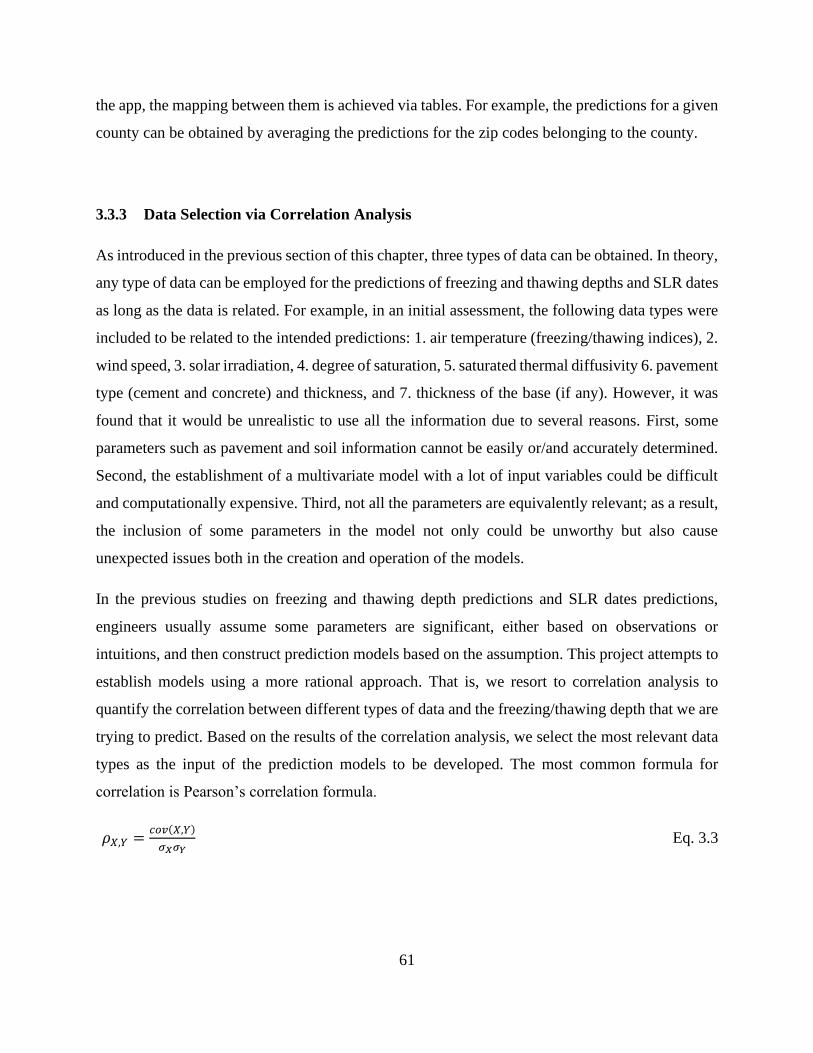
61
the app, the mapping between them is achieved via tables. For example, the predictions for a given
county can be obtained by averaging the predictions for the zip codes belonging to the county.
3.3.3 Data Selection via Correlation Analysis
As introduced in the previous section of this chapter, three types of data can be obtained. In theory,
any type of data can be employed for the predictions of freezing and thawing depths and SLR dates
as long as the data is related. For example, in an initial assessment, the following data types were
included to be related to the intended predictions: 1. air temperature (freezing/thawing indices), 2.
wind speed, 3. solar irradiation, 4. degree of saturation, 5. saturated thermal diffusivity 6. pavement
type (cement and concrete) and thickness, and 7. thickness of the base (if any). However, it was
found that it would be unrealistic to use all the information due to several reasons. First, some
parameters such as pavement and soil information cannot be easily or/and accurately determined.
Second, the establishment of a multivariate model with a lot of input variables could be difficult
and computationally expensive. Third, not all the parameters are equivalently relevant; as a result,
the inclusion of some parameters in the model not only could be unworthy but also cause
unexpected issues both in the creation and operation of the models.
In the previous studies on freezing and thawing depth predictions and SLR dates predictions,
engineers usually assume some parameters are significant, either based on observations or
intuitions, and then construct prediction models based on the assumption. This project attempts to
establish models using a more rational approach. That is, we resort to correlation analysis to
quantify the correlation between different types of data and the freezing/thawing depth that we are
trying to predict. Based on the results of the correlation analysis, we select the most relevant data
types as the input of the prediction models to be developed. The most common formula for
correlation is Pearson’s correlation formula.
𝜌𝑋,𝑌 =𝑐𝑜𝑣(𝑋,𝑌)
𝜎𝑋𝜎𝑌 Eq. 3.3

62
where 𝑋 and 𝑌 are the two variables whose correlation is computed, 𝑐𝑜𝑣(𝑋, 𝑌) is the covariance
of 𝑋 and 𝑌, 𝜎𝑋 is the standard deviation of 𝑋, 𝜎𝑌 is the standard deviation of 𝑌. The covariance is
calculated using the following equation:
𝑐𝑜𝑣(𝑋, 𝑌) = Ε[(𝑋 − 𝜇𝑋)(𝑌 − 𝜇𝑌)] Eq. 3.4
where Ε is the expectation, 𝜇𝑋 is the mean of 𝑋, and 𝜇𝑌 is the mean of 𝑌.
Shown in Figure 3.8 to Figure 3.10 are the correlation analysis results for selected data types at
typical RWIS sites. As can be seen, the correlation coefficient between any variable and itself is
one. The correlation coefficients of interest are the correlation coefficients between the FD/TD and
other data types. It is not difficult the conclude that the pavement temperature has the highest
correlation coefficient with both FD and TD in most cases, followed by the air temperature,
freezing index, and thawing index. Due to this fact, the prediction models for freezing and thawing
depth and SLR dates are built with freezing and thawing indices calculated with the pavement
surface temperature, which is available as an RWIS data type.
1.00
0.08
0.17
NaN
-0.04
0.20
-0.31
0.62
0.34
0.03
-0.32
-0.03
0.15
-0.08
-0.03
0.04
0.04
0.08
1.00
0.96
NaN
-0.10
-0.20
-0.22
-0.05
-0.07
0.97
0.33
-0.15
-0.21
-0.61
-0.10
-0.59
-0.62
0.17
0.96
1.00
NaN
-0.07
-0.21
-0.31
0.04
0.21
0.91
0.22
-0.13
-0.22
-0.57
-0.13
-0.60
-0.63
NaN
NaN
NaN
NaN
NaN
NaN
NaN
NaN
NaN
NaN
NaN
NaN
NaN
NaN
NaN
NaN
NaN
-0.04
-0.10
-0.07
NaN
1.00
0.21
-0.26
0.12
0.05
-0.12
0.16
0.98
0.11
0.04
-0.08
-0.01
0.01
0.20
-0.20
-0.21
NaN
0.21
1.00
-0.37
0.20
-0.06
-0.28
-0.39
0.23
0.97
0.24
0.08
0.23
0.24
-0.31
-0.22
-0.31
NaN
-0.26
-0.37
1.00
-0.34
-0.34
-0.12
0.24
-0.24
-0.33
0.17
0.04
0.09
0.06
0.62
-0.05
0.04
NaN
0.12
0.20
-0.34
1.00
0.35
-0.10
-0.40
0.14
0.13
-0.03
-0.01
-0.01
0.01
0.34
-0.07
0.21
NaN
0.05
-0.06
-0.34
0.35
1.00
-0.15
-0.42
0.04
-0.07
0.06
-0.12
-0.12
-0.10
0.03
0.97
0.91
NaN
-0.12
-0.28
-0.12
-0.10
-0.15
1.00
0.38
-0.17
-0.29
-0.63
-0.12
-0.57
-0.60
-0.32
0.33
0.22
NaN
0.16
-0.39
0.24
-0.40
-0.42
0.38
1.00
0.14
-0.43
-0.24
0.06
-0.12
-0.13
-0.03
-0.15
-0.13
NaN
0.98
0.23
-0.24
0.14
0.04
-0.17
0.14
1.00
0.13
0.09
-0.06
0.03
0.04
0.15
-0.21
-0.22
NaN
0.11
0.97
-0.33
0.13
-0.07
-0.29
-0.43
0.13
1.00
0.25
0.06
0.21
0.22
-0.08
-0.61
-0.57
NaN
0.04
0.24
0.17
-0.03
0.06
-0.63
-0.24
0.09
0.25
1.00
0.42
0.60
0.54
-0.03
-0.10
-0.13
NaN
-0.08
0.08
0.04
-0.01
-0.12
-0.12
0.06
-0.06
0.06
0.42
1.00
0.34
0.31
0.04
-0.59
-0.60
NaN
-0.01
0.23
0.09
-0.01
-0.12
-0.57
-0.12
0.03
0.21
0.60
0.34
1.00
0.99
0.04
-0.62
-0.63
NaN
0.01
0.24
0.06
0.01
-0.10
-0.60
-0.13
0.04
0.22
0.54
0.31
0.99
1.00
Total P
recipita
tion(
mm
)
AirT
emp(C
elsius)
(no:
1)
Dew
Point
Tem
p(Cels
ius) (n
o:1)
Freeze
Tem
p(Celsius
) (no
:1)
Max
Win
d Dire
ction(M
agne
tic D
egre
es) (n
o:1)
Max
Wind S
peed(m
s) (n
o:1)
Press
ure(h
pa) (n
o:1)
Rain In
tensi
ty(m
mh)
(no:
1)
Relat
ive
Hum
idity
(%) (
no:1)
Surface
Tem
p(Cels
ius)
(no:
1)
Visibility(m
) (no
:1)
Wind
Dire
ction(
Mag
netic D
egrees
) (no
:1)
Win
d Spee
d(ms)
(no:1
)
Freez
ing
Dept
h (In
ch)
Thawing D
epth
(Inch
)
Freezi
ng In
dex (°
C d
ays)
Thawing
Inde
x (°C d
ays)
Total Precipitation(mm)AirTemp(Celsius) (no:1)
Dew Point Temp(Celsius) (no:1)Freeze Temp(Celsius) (no:1)
Max Wind Direction(Magnetic Degrees) (no:1)Max Wind Speed(ms) (no:1)
Pressure(hpa) (no:1)Rain Intensity(mmh) (no:1)
Relative Humidity(%) (no:1)Surface Temp(Celsius) (no:1)
Visibility(m) (no:1)Wind Direction(Magnetic Degrees) (no:1)
Wind Speed(ms) (no:1)Freezing Depth (Inch)Thawing Depth (Inch)
Freezing Index (°C days)Thawing Index (°C days) -0.50
0.00
0.50
1.00
-0.50
0.00
0.50
1.00
-0.50
Figure 3.8 Correlation analysis for data selection in predictions of freezing and thawing depths
and SLR dates (Site Fife Lake)

63
1.00
0.01
0.10
NaN
-0.11
0.12
-0.32
0.72
-0.23
0.00
-0.27
-0.11
0.06
-0.04
0.02
0.04
0.04
0.01
1.00
0.96
NaN
-0.02
-0.33
-0.25
-0.04
-0.37
0.95
-0.19
-0.10
-0.31
-0.58
-0.05
-0.60
-0.64
0.10
0.96
1.00
NaN
-0.03
-0.33
-0.33
0.06
-0.39
0.90
-0.29
-0.11
-0.31
-0.53
-0.03
-0.60
-0.63
NaN
NaN
NaN
NaN
NaN
NaN
NaN
NaN
NaN
NaN
NaN
NaN
NaN
NaN
NaN
NaN
NaN
-0.11
-0.02
-0.03
NaN
1.00
0.45
-0.19
0.04
0.08
0.01
0.05
0.97
0.49
-0.07
-0.07
-0.05
-0.05
0.12
-0.33
-0.33
NaN
0.45
1.00
-0.35
0.24
0.35
-0.44
0.04
0.48
0.98
0.22
0.06
0.08
0.12
-0.32
-0.25
-0.33
NaN
-0.19
-0.35
1.00
-0.33
0.09
-0.16
0.17
-0.16
-0.35
0.16
-0.12
0.16
0.13
0.72
-0.04
0.06
NaN
0.04
0.24
-0.33
1.00
-0.16
-0.06
-0.29
0.04
0.18
-0.07
-0.04
-0.03
-0.01
-0.23
-0.37
-0.39
NaN
0.08
0.35
0.09
-0.16
1.00
-0.47
0.14
0.12
0.33
0.34
0.07
0.21
0.23
0.00
0.95
0.90
NaN
0.01
-0.44
-0.16
-0.06
-0.47
1.00
-0.17
-0.07
-0.42
-0.62
-0.09
-0.56
-0.60
-0.27
-0.19
-0.29
NaN
0.05
0.04
0.17
-0.29
0.14
-0.17
1.00
0.09
0.06
-0.11
-0.18
-0.01
0.01
-0.11
-0.10
-0.11
NaN
0.97
0.48
-0.16
0.04
0.12
-0.07
0.09
1.00
0.53
-0.01
-0.06
-0.03
-0.02
0.06
-0.31
-0.31
NaN
0.49
0.98
-0.35
0.18
0.33
-0.42
0.06
0.53
1.00
0.23
0.07
0.07
0.10
-0.04
-0.58
-0.53
NaN
-0.07
0.22
0.16
-0.07
0.34
-0.62
-0.11
-0.01
0.23
1.00
0.33
0.41
0.38
0.02
-0.05
-0.03
NaN
-0.07
0.06
-0.12
-0.04
0.07
-0.09
-0.18
-0.06
0.07
0.33
1.00
0.23
0.19
0.04
-0.60
-0.60
NaN
-0.05
0.08
0.16
-0.03
0.21
-0.56
-0.01
-0.03
0.07
0.41
0.23
1.00
0.99
0.04
-0.64
-0.63
NaN
-0.05
0.12
0.13
-0.01
0.23
-0.60
0.01
-0.02
0.10
0.38
0.19
0.99
1.00
Total P
recipita
tion(
mm
)
AirT
emp(C
elsius)
(no:
1)
Dew
Point
Tem
p(Cels
ius) (n
o:1)
Freeze
Tem
p(Celsius
) (no
:1)
Max
Win
d Dire
ction(M
agne
tic D
egre
es) (n
o:1)
Max
Wind S
peed(m
s) (n
o:1)
Press
ure(h
pa) (n
o:1)
Rain In
tensi
ty(m
mh)
(no:
1)
Relat
ive
Hum
idity
(%) (
no:1)
Surface
Tem
p(Cels
ius)
(no:
1)
Visibility(m
) (no
:1)
Wind
Dire
ction(
Mag
netic D
egrees
) (no
:1)
Win
d Spee
d(ms)
(no:1
)
Freez
ing
Dept
h (In
ch)
Thawing D
epth
(Inch
)
Freezi
ng In
dex (°
C d
ays)
Thawing
Inde
x (°C d
ays)
Total Precipitation(mm)AirTemp(Celsius) (no:1)
Dew Point Temp(Celsius) (no:1)Freeze Temp(Celsius) (no:1)
Max Wind Direction(Magnetic Degrees) (no:1)Max Wind Speed(ms) (no:1)
Pressure(hpa) (no:1)Rain Intensity(mmh) (no:1)
Relative Humidity(%) (no:1)Surface Temp(Celsius) (no:1)
Visibility(m) (no:1)Wind Direction(Magnetic Degrees) (no:1)
Wind Speed(ms) (no:1)Freezing Depth (Inch)Thawing Depth (Inch)
Freezing Index (°C days)Thawing Index (°C days) -0.50
0.00
0.50
1.00
-0.50
0.00
0.50
1.00
-0.50
Figure 3.9 Correlation analysis for data selection in predictions of freezing and thawing depths
and SLR dates (Site Eastport)
1.00
0.09
0.16
-0.07
-0.01
0.29
-0.06
0.44
0.22
0.03
0.17
0.02
0.28
-0.06
-0.07
-0.06
-0.06
0.09
1.00
0.96
0.43
-0.45
-0.31
-0.00
0.04
-0.05
0.98
-0.54
-0.44
-0.28
-0.53
-0.39
-0.45
-0.39
0.16
0.96
1.00
0.38
-0.48
-0.34
-0.06
0.11
0.11
0.92
-0.54
-0.46
-0.31
-0.52
-0.41
-0.46
-0.41
-0.07
0.43
0.38
1.00
-0.23
-0.25
-0.16
0.02
-0.30
0.44
-0.35
-0.22
-0.23
-0.27
-0.16
-0.21
-0.17
-0.01
-0.45
-0.48
-0.23
1.00
0.62
0.26
0.09
0.12
-0.45
0.74
0.98
0.58
0.28
0.23
0.27
0.25
0.29
-0.31
-0.34
-0.25
0.62
1.00
0.23
0.16
0.08
-0.37
0.71
0.64
0.98
0.24
0.21
0.22
0.21
-0.06
-0.00
-0.06
-0.16
0.26
0.23
1.00
0.04
0.62
0.04
0.31
0.24
0.22
0.10
0.08
0.09
0.08
0.44
0.04
0.11
0.02
0.09
0.16
0.04
1.00
0.27
-0.01
0.21
0.11
0.15
-0.15
-0.12
-0.15
-0.14
0.22
-0.05
0.11
-0.30
0.12
0.08
0.62
0.27
1.00
-0.08
0.26
0.11
0.06
0.07
-0.02
0.01
-0.02
0.03
0.98
0.92
0.44
-0.45
-0.37
0.04
-0.01
-0.08
1.00
-0.59
-0.44
-0.34
-0.54
-0.39
-0.46
-0.40
0.17
-0.54
-0.54
-0.35
0.74
0.71
0.31
0.21
0.26
-0.59
1.00
0.71
0.67
0.30
0.23
0.26
0.23
0.02
-0.44
-0.46
-0.22
0.98
0.64
0.24
0.11
0.11
-0.44
0.71
1.00
0.60
0.28
0.25
0.28
0.27
0.28
-0.28
-0.31
-0.23
0.58
0.98
0.22
0.15
0.06
-0.34
0.67
0.60
1.00
0.25
0.20
0.23
0.21
-0.06
-0.53
-0.52
-0.27
0.28
0.24
0.10
-0.15
0.07
-0.54
0.30
0.28
0.25
1.00
0.78
0.95
0.88
-0.07
-0.39
-0.41
-0.16
0.23
0.21
0.08
-0.12
-0.02
-0.39
0.23
0.25
0.20
0.78
1.00
0.84
0.87
-0.06
-0.45
-0.46
-0.21
0.27
0.22
0.09
-0.15
0.01
-0.46
0.26
0.28
0.23
0.95
0.84
1.00
0.98
-0.06
-0.39
-0.41
-0.17
0.25
0.21
0.08
-0.14
-0.02
-0.40
0.23
0.27
0.21
0.88
0.87
0.98
1.00
Total P
recipita
tion(
mm
)
AirT
emp(C
elsius)
(no:
1)
Dew
Point
Tem
p(Cels
ius) (n
o:1)
Freeze
Tem
p(Celsius
) (no
:1)
Max
Win
d Dire
ction(M
agne
tic D
egre
es) (n
o:1)
Max
Wind S
peed(m
s) (n
o:1)
Press
ure(h
pa) (n
o:1)
Rain In
tensi
ty(m
mh)
(no:
1)
Relat
ive
Hum
idity
(%) (
no:1)
Surface
Tem
p(Cels
ius)
(no:
1)
Visibility(m
) (no
:1)
Wind
Dire
ction(
Mag
netic D
egrees
) (no
:1)
Win
d Spee
d(ms)
(no:1
)
Freez
ing
Dept
h (In
ch)
Thawing D
epth
(Inch
)
Freezi
ng In
dex (°
C d
ays)
Thawing
Inde
x (°C d
ays)
Total Precipitation(mm)AirTemp(Celsius) (no:1)
Dew Point Temp(Celsius) (no:1)Freeze Temp(Celsius) (no:1)
Max Wind Direction(Magnetic Degrees) (no:1)Max Wind Speed(ms) (no:1)
Pressure(hpa) (no:1)Rain Intensity(mmh) (no:1)
Relative Humidity(%) (no:1)Surface Temp(Celsius) (no:1)
Visibility(m) (no:1)Wind Direction(Magnetic Degrees) (no:1)
Wind Speed(ms) (no:1)Freezing Depth (Inch)Thawing Depth (Inch)
Freezing Index (°C days)Thawing Index (°C days)
-0.50
0.00
0.50
1.00
Figure 3.10 Correlation analysis for data selection in predictions of freezing and thawing depths
and SLR dates (Site Cadillac South)

64
Chapter 4 Multivariate Freezing-Thawing Depth Prediction Model
4.1 Overview
Road damages induced by heavily loaded truck traffic during the spring thaw are major road
distress in cold regions. To minimize these damages, Spring Load Restriction (SLR) is widely
applied in the U.S., Canada, and other countries during the early thawing season by controlling the
movement of freight-carrying trucks and heavy equipment travel until the thawing ends. Most SLR
policies rely on the Freezing Depth (FD) and Thawing Depth (TD), especially the latter one.
Therefore, accurate predictions of FD and TD are important to prevent both the extensive damage
to the pavement due to the late placement or early removal of SLR and the economic loss of road
users due to an unnecessarily long SLR period. Here, we propose a new multivariate model for
predicting FD and TD in support of SLR decision-making. The model gives a curving surface of
FD and TD in a 3-dimensional space, instead of 2-dimensional in traditional methods, by
considering both the freezing and thawing indices in the entire freeze-thaw cycle. For model
evaluations, yearly field data measured at five typical sites from 104 sites in Michigan were
adopted. The evaluation results showed that the proposed model is accurate in predicting FD and
TD for most sites. Compared to the previous TD predictions in the existing study, the TD
predictions with the proposed model have been significantly improved. In addition, this study
provides field data that have not been reported earlier in the literature and that can be used for
validating other prediction models. The reported work is ready for practice for roadways in cold
regions to support SLR decision-making.
In this chapter, we propose a new multivariate FD/TD prediction model, which is easily
implementable for supporting SLR decision-making. The proposed model is primarily evaluated
using field data measured at five typical sites in Michigan. The evaluation results for FD and TD
based on both FI and TI in a 3-dimensional space are presented and discussed.
4.2 Field Measurements
Michigan Department of Transportation (MDOT) deployed a Road Weather Information System
(RWIS) to measure road and weather conditions on highways and communicate this information

65
to users in a maintenance facility. Through a series of strategically placed Environmental Sensor
Stations (ESSs) in the RWIS, key road and weather conditions (e.g., humidity, wind speed, average
air temperature, and temperatures of the pavement surface and subsurface) are measured in real-
time. To share yearly RWIS data in public, we developed the MDOT SLR website
(https://mdotslr.org/). As of now, there are 104 sites implemented with ESSs in Michigan as shown
in Figure 4.1. The RWIS data for these sites can be freely downloaded from the MDOT SLR
website.
In this study, we primarily selected five typical sites for analyses, three from the Upper Peninsula
and two in the Lower Peninsula.
Figure 4.1 Overview of monitored sites with ESSs in Michigan
The pavement structure of the five selected sites primarily consists of an asphalt/concrete surface,
a granular base, and a soil sub-base. Details of the pavement structure, soil types, and properties
can be found in Baladi and Rajaei (2015). Table 4.1 shows all the measured temperatures needed
for this study. The air temperature was measured by the air temperature sensor, while the pavement

66
surface and base temperatures were measured by surface and subsurface sensors, respectively. For
base temperatures, 15 subsurface sensors were used to measure the temperatures from the base
surface to a depth of 72 inches (1.83 m), which can be used to calculate FD and TD.
Table 4.1 Needed parameters for analyses
Material Measured temperature
Air Average temperature (°C)
Pavement
Surface temperature (°C)
Base
temperature
(°C)
Depth from base surface (inch)
0 3 6 9 12 18 24 30 36 42 48 54 60 66 72
Note: 1 inch=2.54 cm
4.3 A New Freezing-Thawing Depth Prediction Model
Calculations of FD and TD are related to the solution to a phase-change (ice-liquid) problem of
heat transfer. In a pioneering study, Neumman solved FD by analyzing the 1D heat transfer in a
semi-infinite soil (Jiji and Ganatos 2009). FD in the Neumman’s equation is a function of the
surface temperature, time, and thermal conductivities of both the frozen and unfrozen soils (see
details in Baladi and Rajaei (2015)). A special case of the Neumman’s equation was further solved
by assuming no heat transfer in the liquid (Baladi and Rajaei 2015), in which FD is formulated by
𝐹𝐷 = √2𝜆𝑓
𝜌𝑙(𝑇0 − 𝑇𝑠,𝑠)𝑡 Eq. 4.1
where 𝜆𝑓 is the thermal conductivity of a frozen soil (W/(m oC)), 𝜌 is the soil density (kg/m3), 𝑙 is
the latent heat of fusion (J/kg), 𝑇0 is the freezing point of bulk water (=0 oC), 𝑇𝑠,𝑠 is the soil surface
temperature, and 𝑡 is the time (day). Based on Eq. 4.1, many physico-empirical models were
further developed. These physico-empirical models share a common form of Eq. 4.2 to calculate
FD (Aldrich and Paynter 1953)

67
𝐹𝐷 = 𝑎𝑜√48𝜆𝑓𝑛𝐹𝐼
𝐿 Eq. 4.2
where 𝐿 is the volumetric latent heat of fusion (J/m3), 𝑛 is a dimensionless parameter converting
the air temperature index to the surface temperature index, 𝑎𝑜 is a dimensionless correction factor
considering the initial freezing depression (Berg et al. 2006).
The recent physico-empirical models (Asefzadeh et al. 2016; Baïz et al. 2008; Marquis
2008; Miller et al. 2012) further loosened the constraints in Eq. 4.2 by only keeping FI and lumping
all the other terms with physical meanings into one or two fitting constants. The fitting constants
can be obtained by linear regression with measured data. Therefore, physico-empirical models are
also statistical models. One major feature of these physico-empirical models is the linear
relationship between FD and the square root of FI. The above existing studies have proved that
satisfactory predictions for FD can be made using the square root of FI. This study also uses this
method for the FD prediction with the square root of FI. In addition, results from the field
measurements for the five selected sites and additional sites, shown in Fig. 4, clearly indicate that
FD follows a square root function decay as TI increases.
Figure 4.2 Field measurement results of TI-FD relationships from ten sites in Michigan
Considering the above facts, the following model is proposed for FD involving both FI and TI

68
𝐹𝐷 = 𝑎√𝐹𝐼 + √𝑐 − 𝑏𝑇𝐼 + 𝑑 Eq. 4.3
where a, b, c, and d are fitting constants, the first three always positive. It is known that freezing
and thawing processes are similar (Konrad 1989); as a result, the mathematical formulations for
TD and FD are similar
𝑇𝐷 = −𝑒√𝐹𝐼𝑇 − √𝑔 − 𝑓𝑇𝐼 + ℎ Eq. 4.4
where e, g, f, and h are fitting constants, the first three always positive. FIT is the cumulative
freezing index in the thawing period only. FI is not adopted here for TD, as FI mainly represents
the cumulative frost in the pavement base during the freezing period, which in fact is irrelevant to
TD. Therefore, FIT is adopted, which can appropriately consider the cumulative freezing index
when the thawing starts. The fitting constants for FD and TD reflect the real situation for the depth
and duration of the freeze and/or thaw penetration in the pavement base. The fitting constants can
be obtained using the nonlinear least-squares method on each site. It is noted that 𝑐 − 𝑏𝑇𝐼 > 0 and
𝑔 − 𝑓𝑇𝐼 > 0 should be ensured (i.e., the principal square root of a positive number) in the
nonlinear regression analysis.
The cumulative freezing index during the freezing period can be calculated based on 𝑇0 = 0 ∘𝐶
over a given period
{𝐹𝐼 = ∑(𝑇0 − 𝑇𝑠)𝑇0 − 𝑇𝑠 < 0 ⇒ 𝑇0 − 𝑇𝑠 = 0
Eq. 4.5
where 𝑇𝑠 is the pavement surface temperature. Similarly, FIT can be calculated using Eq. 4.5
starting from the date when the first TD occurs in the thawing period. The cumulative thawing
index is computed by
{𝑇𝐼 = ∑(𝑇𝑠 − 𝑇𝑟𝑒𝑓)
𝑇𝑠 − 𝑇𝑟𝑒𝑓 < 0 ⇒ 𝑇𝑠 − 𝑇𝑟𝑒𝑓 = 0 Eq. 4.6

69
where 𝑇ref is the reference temperature to account for the amount of solar radiation and thermal
properties of the pavement material. In this study, 𝑇𝑟𝑒𝑓 = −1.67 ∘𝐶 was used according to the
guideline of FHWA-WSDOT (Mahoney et al. 1987). Eq. 4.5 and Eq. 4.6 use the pavement surface
temperature instead of the average air temperature. This is due to the fact that FI and TI calculated
with the average air temperature failed to correlate FD and TD in the freeze-thaw cycle (see Error!
Reference source not found.), which will be discussed later in detail.
Figure 4.3 Schematic of 3D model and its project on the FD plane

70
Figure 4.4 Schematic of 3D model and its project on the TD plane
4.4 Prediction and Evaluation of Freezing-Thawing Depth Model
FDs and TDs presented in Figure 3.4 for all the selected sites were used for the statistical analyses
based on the proposed model using FI and TI values calculated with the pavement surface
temperature. Error! Reference source not found.a shows the fitting result of FD for Harvey. A
curving surface for predicted FD is exhibited, in which FD increases as FI increases and decreases
as TI increases. The maximum FD could be obtained when FI almost remains unchanged and TI
significantly increases. The predicted FD surface is in good agreement with the measured FDs and
the coefficient of determination is found to be 0.94. Therefore, the proposed FD model performs
well in predicting FD with high accuracy.
Fig. 10b presents the surface fitting result of TD formulated by TI and FIT for Harvey. We can
clearly see that the predicted TD surface is very close to the measured TDs. TD increases with an
increase in TI. However, it is difficult to observe how TD changes with FIT from Error!
Reference source not found.b, as Point A does not belong to TD data in the thawing period. This
point appears before February 2018 due to the occurrence of some warm days in the freezing
period (see Figure 3.4a). As our goal is to predict TD in the thawing period for applying SLR,
Point A beyond the thawing cycle in Figure 3.4a can be removed. It can be seen in Error!
Reference source not found.c that TD decreases as FIT increases when Point A is excluded. The
predicted TD surface fitted to the measured TDs in the thawing cycle becomes more accurate and
the coefficient of determination increases from 0.83 to 0.90 accordingly.

71
Figure 4.5 Fitting surfaces for Harvey: (a) FD fitting, (b) TD fitting with the whole TD data, (c)
TD fitting with the thawing cycle data.
For the other four sites, Error! Reference source not found. presents the 3-dimensional fitting
surfaces of FD and TD. The TD data in the thawing cycle in Fig. 8 were used for fitting TD for
each site. It can be seen that the predicted FD surfaces for these sites match well with the
measured FDs. The coefficient of determination for most sites is found to be as high as 0.93. For
TD predictions, the predicted TD surfaces for Michigamme and Glennie are in good agreement
with the measured TDs (see Error! Reference source not found.a and Error! Reference
source not found.d). The predicted TD surfaces for the other two sites are not as good as those

72
for Harvey and Michigamme, as shown in Error! Reference source not found.b and Error!
Reference source not found.c. The reason is that the measured TDs do not increase
continuously, but rather, go up and down, for example, Charlevoix in Figure 3.4c. This makes it
difficult to fit a 3-dimensional surface in the nonlinear regression analysis. However, the
predicted TD surfaces for these two sites capture the key mechanism of the TD-TI-FIT
relationship, i.e., TD nonlinearly increases with an increase in TI and a decrease in FIT. Also,
from the fitting constants tabulated in Figure 4.6 Fitting surfaces for FD and TD: (a)
Michigamme, (b) Seney, (c) Charlevoix, and (d) Glennie
, each fitting constant has the same sign for all the selected sites, regardless of FD and TD
predictions. This implies that the FD-FI-TI relationship for all the five selected sites has the same
trend, so is that of the TD-TI-FIT relationship. The proposed model was further assessed by
additional sites shown in Figure 4.3. The 3-dimensional fitting surfaces for these additional sites
are very similar to those in Error! Reference source not found.. The fitting results for these
additional sites are tabulated in Table 3. It is seen that the coefficient of determination for FD and
TD for most sites is higher than 0.8, which further confirms that the proposed model is adaptable
to other sites. The above evaluation results clearly show the key varying mechanisms of both the
FD-FI-TI relationship and the TD-TI-FIT relationship, and also demonstrate the high accuracy of
the proposed model for predicting FD and TD for most sites. Comprehensive lists of the fitting
constants for the RWIS sites, which are termed as FD/TD prediction models for these sites, were
obtained based on the RWIS data in Year 2017-2018 and Year 2018-2019, and the lists are
provided in the Appendix.

73

74
Figure 4.6 Fitting surfaces for FD and TD: (a) Michigamme, (b) Seney, (c) Charlevoix, and (d)
Glennie
Table 4.2 Fitting results for the five selected sites
Site Variable prediction Fitting constant
unit: inch oC-day-0.5 inch2 oC-day-1 inch2 inch
Harvey
FD a b c d R2
4.03 69.24 14574 -109.5 0.94
TD e f g h R2
TD with whole data 0.17 56.59 1717.91 71.9 0.83
TD with thawing cycle 5.11 120.3 18422.1 94.93 0.9
Michigamme
FD
a b c d R2
2.56 36.84 6913.6 -78.34 0.93
TD with thawing cycle e f g h R2
6.31 229.7 19071 100.1 0.92
Seney
FD a b c d R2
2.67 29.06 8028.8 -78.81 0.78
TD with thawing cycle e f g h R2
8.16 50.8 5410.8 42.27 0.54
Charlevoix FD a b c d R2
3.15 17.09 528.36 -65.47 0.93

75
TD with thawing cycle e f g h R2
5.43 29.03 1126.04 69.2 0.51
Glennie
FD a b c d R2
3.60 39.78 215.31 -64.56 0.87
TD with thawing cycle e f g h R2
11.90 35.69 688.92 51.99 0.87
Note that 1 inch=2.54 cm
ennie
Seney
Michigamme
arvey
Char evoi
Rudard
Au Train
Cadi ac South
astport
Fife a e
Figure 4.3 Locations of additional sites in Michigan
Table 4.2 Prediction results for additional sites
Site Variable prediction Fitting constant
unit: inch oC-day-0.5 inch2 oC-day-1 inch2 inch
Rudyard
FD a b c d R2
2.36 7.08 2790.05 -69.93 0.96
TD with thawing cycle e f g h R2
1.19 20.30 2033.04 83.42 0.83
Eastport FD a b c d R2

76
3.37 13.39 460.14 -65.84 0.83
TD with thawing cycle e f g h R2
0.56 70.37 1339.69 68.11 0.80
Au Train
FD a b c d R2
3.16 51.25 427.50 -76.16 0.84
TD with thawing cycle e f g h R2
2.70 11.11 204.37 36.92 0.54
Cadillac South
FD a b c d R2
0.83 0.91 233.98 -13.39 0.87
TD with thawing cycle e f g h R2
0.32 1.70 210.58 22.88 0.85
Fife Lake
FD a b c d R2
3.80 27.25 383.19 -90.74 0.92
TD with thawing cycle e f g h R2
11.00 23.10 388.24 58.94 0.84
1 inch=2.54 cm
4.5 Discussions
4.5.1 Calculations of FI and TI via Surface Temperature Rather than Air Temperature
Calculations of FI and TI are needed to accurately predict FD and TD. To obtain appropriate FI
and TI, the pavement surface temperature was used in this study. This is different from most
existing models (e.g., Baïz et al. (2008) and Chapin et al. (2012)) that adopt the average air
temperature to calculate FI and TI. To illustrate the advantage of using the pavement surface
temperature, Figure 4.4 shows the comparisons of FI and TI calculated with the pavement surface
temperature and those calculated with the average air temperature for Harvey and Michigamme,
in which the corresponding FD and TD are also plotted.
It is clearly seen in Figure 4.4 that when the thawing starts from March 2018, FI calculated with
the average air temperature (dashed blue line) still increases. At the same time, FD significantly
decreases and TD continuously increases. Starting from March 2018, it is also seen that TI
calculated with the air temperature (dashed red line) almost remains unchanged, which does not

77
appear reasonable. When the thawing starts, TI should increase accordingly and FI should
decrease, as the increase in TD is mainly attributed to the continuous thaw penetration in the
pavement base. This causes the accumulated frost in the base to thaw and accordingly, FD should
decrease significantly. FI and TI calculated with the air temperature, however, fail to match the
changes in TD and FD in a realistic way. When the pavement surface temperature is applied, as
shown in Figure 4.4, FI (solid blue line) almost remains unchanged and TI (solid red line) increases
starting from March 2018, which matches very well with the corresponding changes in TD and
FD. In addition to the above two sites, FI and TI calculated with the pavement surface temperature
for the rest of the three sites also match quite well with the trends of FD and TD. Therefore, the
pavement surface temperature is more suitable to calculate FI and TI for predicting FD and TD
than the average air temperature.
Figure 4.4 Comparisons of FI/TI calculated with the pavement surface temperature and the
average air temperature: (a) Harvey and (b) Michigamme

78
4.5.2 Prediction Improvement
Good predictions for both FD and TD, especially the latter one, can be obtained with the proposed
model. The 3D fitted surfaces hide the underneath measured data, causing a difficulty in visually
evaluating the prediction accuracy. To clearly see the predictions, taking the Harvey site for
example, Figure 4.5 shows the fitted line instead of fitted surfaces for both FD and TD. We can
see in Figure 4.5 that the fitted line for FD agrees well with the measured FDs in a 3D space. The
fitted line for TD in Fig. 14b is also very close to the measured TDs, in which the “staircase shape”
is observed. This is due to the fact that TI keeps unchanged and in the meantime FIT increases if
there have a few freezing days during the thawing period, and vice versa.
Figure 4.5 Fitting lines for Harvey: (a) FD fitting, (b) TD fitting with the thawing cycle data
The good predictions with the proposed model are primarily attributable to three reasons. First, the
pavement surface temperature is used to reflect more realistic pavement thermal conditions than
the air temperature, as explained in Section 4.5.1. Second, the proposed model adopts the
mathematical form of −√𝑔 − 𝑓𝑇𝐼 for TD predictions rather than the general form of 𝑓√𝑇𝐼 used
in the existing studies (e.g., Baïz et al. (2008)). The latter one may be only suitable for a specific
site, while the former one has been confirmed by many different sites shown in Figure 4.3. Third,
the proposed model adopts FIT rather than FI for predicting TD. The selection of FIT is more
reasonable because the value of FI also determines the TD prediction accuracy in addition to its

79
mathematical form (i.e., square root). Therefore, FIT is better than FI for the TD prediction by
appropriately considering the cumulative freezing index when the thawing starts.
Though the FD and TD predictions are promising for most sites in this study, there are still
deviations for a few sites, e.g., Seney in Error! Reference source not found.b. The possible
reason is that factors, such as solar radiation and thermal properties of pavement materials, are not
considered directly, but instead, considered via a constant 𝑇ref. The effect of the solar radiation is
believed to be significant as the solar radiation can significantly change both the pavement surface
and air temperatures. However, the proposed model can predict both FD and TD with high
accuracy for most sites even using a constant 𝑇ref. Fig. 15 presents the comparison between the
previous TD predictions (Baladi and Rajaei 2015) in Michigan and those with the proposed model.
In addition to the selected five typical sites, three additional sites were also analyzed to evaluate
the predicted maximum TDs. We can clearly see that the TD predictions in this study are very
close to the measured TDs and much better than the previous TD predictions (Baladi and Rajaei
2015). Therefore, the TD predictions have been significantly improved.
Figure 4.6 Comparison of the maximum measured TDs and predicted TDs

80
4.6 Conclusions
This study proposes a new multivariate model for predicting FD and TD to support SLR decision-
making. The model can give a curving surface of FD and TD in a 3-dimensional space by
considering both the freezing and thawing indices. For the model evaluation, yearly field data
measured at five typical sites from 104 sites in Michigan were used. The results indicated that the
use of the pavement surface temperature gives reasonable FI and TI and better results than the
average air temperature. FI and TI calculated with the pavement surface temperature match well
with the corresponding changes in FD and TD with time. Therefore, the pavement surface
temperature is more appropriate to calculate FI and TI for FD and TD predictions.
Evaluation of the results from the proposed model revealed that FD can be predicted with high
accuracy for all the selected sites. For the FD-FI-TI relationship, the 3-dimensional surface clearly
demonstrated that FD increases as FI increases and decreases as TI increases in the freeze-thaw
cycle. The predicted TDs for three selected sites are very close to the measured TDs. There are
deviations in the TD predictions for the other two sites, which is possibly due to the fact that
factors, e.g., solar radiation and thermal properties of pavement materials, are not considered
directly during the thawing period. However, the TD predictions have been significantly improved
when compared to the previous TD predictions. Therefore, the proposed model is a capable tool
for practice for roadways in cold regions in support of SLR decision-making. In addition, the
present study provides field data that have not been reported earlier in the literature and that can
be used for validating other prediction models.

81
Chapter 5 Freezing-Thawing Depth Prediction with Constrained
Optimization for Applications of Spring Load Restriction
5.1 Overview
Spring Load Restriction (SLR) has been widely implemented in many countries to reduce the cost
of road repair for freeze-thaw induced damages in cold regions occurring in the spring thawing
season. In most SLR policies, accurate predictions of the Freezing Depth (FD) and Thawing Depth
(TD) are very critical because both FD and TD directly determine the dates for the SLR placement
and removal. In this study, we propose a new constrained optimization approach to predict FD and
TD and evaluate this approach for making SLR decisions with field measurements collected at
four sites during two adjacent year cycles. The evaluation results showed that constrained
optimization can not only accurately predict FD and TD with the determination coefficient of
higher than 0.91 for most sites, but enable FD to meet TD in the thawing season for accurate SLR-
decision making, which, however, cannot be achieved using non-constrained optimization widely
adopted in the literature. We also discuss the accuracy of using a Thawing Index (TI)/Freezing
Index (FI) ratio of 0.3 that still has been used by several agencies in the U.S. to determine the
removal date of SLR. Our results indicated that on the true dates of the SLR removal, a TI/FI ratio
is not equal even close to 0.3 for most sites. By comparison, a TI/FI ratio of 0.3 will be less accurate
than the FD and TD prediction model for SLR decision-making. The methodology reported in this
study is easy to use and implement for road engineers and the insights will help make accurate
SLR decisions to prevent roads in cold regions from freeze-thaw induced damages.
5.2 Introduction
Many FD and TD prediction models have been proposed in the literature based on 1D heat transfer
in a semi-infinite soil. The typical one is the Neumann’ empirical model (Jiji and Ganatos 2009),
where FD is predicted in terms of the square root of FI and soil properties (e.g., thermal
conductivity). The following models make some modifications by only keeping FI and lumping
all the other terms for soil properties into one or two fitting constants (Asefzadeh et al. 2016; Baïz
et al. 2008; Marquis 2008; Miller et al. 2012). To obtain these fitting constants, nonlinear

82
regression of the measured data is usually employed. For TD predictions, two major types of
prediction models are available in the literature, but each contains 2-4 fitting constants that need
to be determined by nonlinear regression as well. The first type is to predict TD via TI only using
a power function. Chapin et al. (2012), for instance, used this type to predict TD with the measured
data, where the obtained determination coefficient was 0.59-0.83. For the second type, TD is
assumed to share the same mathematical function as that of FD, i.e., the square root of both FI and
TI (see Figure 5.1). In comparison, the determination coefficient obtained based upon the second
type (Baïz et al. 2008) is higher than of the first type and about 0.99. However, Baïz et al. (2008)
predicted TD in the freezing and thawing seasons separately using a piecewise function, which is
inconvenient in practice. Bao et al. (2019) thus suggested using an integrated approach to predict
TD in the whole freeze-thaw cycle using a multivariate model (i.e., a variation of the second type),
in which the obtained determination coefficient is in a range of 0.8-0.94 and the pavement surface
temperature is confirmed to be better than the air temperature for calculating FI and TI.
Figure 5.1 Measured vs predicted data for FD and TD [data is from (Baïz et al. 2008)]. Note
that predicted TD and FD trends are obtained using the thawing season fitting constants.
Though either TI or an FD/TD prediction model has been extensively applied for SLR decision-
making, two issues are still unclear. Firstly, several agencies in the U.S. still use a ratio of 0.3
between TI and FI proposed by Mahoney et al. (1987) to determine the removal date of SLR

83
because of its simplicity. However, it is still uncertain how accurately the TI/FI ratio method
performs for SLR decision-making when compared to an FD/TD prediction model. Secondly, the
essential step in SLR decision-making with an FD/TD prediction model is to determine a date for
the SLR removal when FD meets TD (see Fig. 4 for details) in the thawing season (Baïz et al.
2008). However, FD and TD predicted via the existing model (Baïz et al. 2008) cannot meet with
each other, as shown in Figure 5.1, which hinders the application of the FD and TD prediction
model in practice for SLR decision-making. In addition, when both FI and TI are equal to zero,
FD and TD in the thawing season in Figure 5.1 are 145 and -848 cm, respectively (22.1 and 0.494
cm in the freezing season). These numbers, in fact, should be identical and have the physical
meaning that is related to the pavement surface thickness (see details in Section 5.3.2). Therefore,
the fitting constants in Baïz et al. (2008) are only statistical numbers without clarifying their
physical meaning, which fail to reflect realistic pavement FD and TD conditions.
In this study, we address the above issues using the multivariate FD/TD prediction model adopted
from our previous study (Bao et al. 2019). Though the prediction model used in this study is the
same as that of Bao et al. (2019), there are two distinct differences in the model application. First,
we clearly clarify the physical meaning of all fitting constants in the prediction model. Second, we
propose a new constrained optimization approach for obtaining fitting constants to reflect realistic
pavement FD and TD conditions. We evaluate FD and TD predictions with constrained
optimization via site measurements collected during two adjacent year cycles in Michigan.
Discussion is also made to shed light on the advantages of constrained optimization newly
proposed in this study and how accurate the FD/TD prediction model or a TI/FI ratio is for SLR
decision-making.
5.3 Theory and Method
5.3.1 Field Measurements and SLR Determination Method
Field measurements for road pavements in Michigan are adopted in this study. A Road Weather
Information System (RWIS) deployed in Michigan measures and transmits weather and road
conditions in real-time via various sensors (Figure 5.2). Meteorological sensors record weather

84
conditions, e.g., air temperature, relative humidity, and precipitation. Pavement sensors measure
road conditions, e.g., pavement surface and subsurface temperatures. There are 105 sites in total
and we adopt four typical sites of Michigamme and Seney in the Upper Peninsula and Eastport
and Fife Lake in the Lower Peninsula for analyses.
Figure 5.2 Monitoring sites in Michigan and selected sites location for analyses. Data is from
the Michigan SLR website (https://mdotslr.org)
Figure 5.3 shows the cross-section of the test road pavements. The asphalt/concrete pavement
surface has a thickness of about 25 cm, which is the same as that of roads in Asefzadeh et al.
(2016). Base and subgrade soils are beneath the surface, where the base thickness is about 17 cm.
The major soil type in the four sites is different, i.e., clayey soils in Eastport and Fife Lake and
sandy soils in Michigamme and Seney. FD and TD are not measured directly, but rather calculated
based on the measured subsurface temperatures starting from the base surface to subgrade soils.
The measured locations are 0, 3 (7.62), 6 (15.24), 9 (22.86), 12 (30.48), 18 (45.72), 24 (60.96), 30
(76.2), 36 (91.44), 42 (106.68), 48 (121.92), 54 (137.16), 60 (152.4), 66 (167.64), and 72 inches
(182.88 cm). To calculate FD and TD, two adjacent measured temperatures are compared and the
linear interpolation is used. The base surface in Figure 5.3 is assumed as a datum, below which
FD and TD are positive.

85
Figure 5.3 Schematic of a test road pavement cross section
The placement and removal of SLR are determined according to the suggested theory by Baïz et
al. (2008) and Chapin et al. (2012). As shown in Figure 5.4, the SLR placement takes place if there
are continuous TDs (red square); SLR ends after TD meets FD (purple square). At this time, a
yearly freeze-thaw cycle can be assumed to be complete.
Figure 5.4 SLR decision-making based on the theory proposed by (Baïz et al. 2008)
In general, agencies require a notice at least 5 days prior to the placement and removal of SLR. To
apply the FD/TD prediction model to practical SLR decision-making, Figure 5.5 presents a brief
flowchart suggesting how this could be done. Based on the real-time field data, FD and TD can be
calculated. When the thawing starts and TD continuously increases to a predefined threshold, SLR

86
can be set. SLR will be removed when FD meets TD or reaches other pre-specified thresholds.
The decision to remove SLR can be easily made by observing the FD and TD graphs obtained by
the prediction model. At each site, SLR decisions can be made based on the present FD/TD
prediction models.
Figure 5.5 Conceptual flowchart of the FD/TD prediction model implementation for SLR
5.3.2 Freeze-Thaw Depth Prediction Model with Constrained Optimization
Accurate predictions of FD and TD are very significant for SLR decision-making to notify the
public of SLR postings at least 3 to 5 days in advance for avoiding the economic loss of road users
due to an unnecessarily long SLR period. In this chapter, we adopt the multivariate FD/TD
prediction model that presents high-accuracy predictions of FD and TD explained in the previous
chapter (Bao et al. 2019). This model assumes that FD is a function of the square root of both FI
and TI as
𝐹𝐷 = 𝑎√𝐹𝐼 + √𝑐 − 𝑏𝑇𝐼 − 𝑑 Eq. 5.1

87
where a, b, c, and d are fitting constants, all are always positive. The mathematical formulation for
TD uses the square root function using the following expression by assuming that freezing and
thawing processes in soils are similar (Konrad 1989)
𝑇𝐷 = −𝑒√𝐹𝐼𝑇 − √𝑔 − 𝑓𝑇𝐼 + ℎ Eq. 5.2
where e, g, f, and h are fitting constants, all are always positive. FIT is the cumulative freezing
index in the thawing period only, which is calculated starting from the first TD data point. Detailed
calculations of FI, FIT, and TI can be found in Section 3.2.4.
Each of Eq. 5.1 and Eq. 5.2 has four fitting constants. For FD, a and b are the lumped parameters
in the freezing and thawing seasons, respectively, to consider the volumetric latent heat of fusion,
the conversion from the air temperature to the surface temperature, and the initial freezing
depression (Aldrich and Paynter 1953; Berg et al. 2006). These two lumped fitting constants reflect
the real situation for the depth and duration of the freeze and thaw penetration in the base and
subgrade soils. Similarly, e and f for TD are also the lumped parameters that have a similar physical
meaning to that of a and b.
The physical meaning of c and d in Eq. 5.1 is related to the pavement surface thickness. Before
the freezing season starts, it is known that both FI and TI are equal to zero. Eq. 5.1 thus can be
rewritten as
𝐹𝐷𝑖𝑛𝑖 = √𝑐 − 𝑑 Eq. 5.3
where 𝐹𝐷𝑖𝑛𝑖 the initial freezing depth to represent the pavement surface thickness. In Figure 5.3,
the base surface is the datum. FD starts from zero in the early freezing stage when FI is slightly
greater than zero and TI is equal to zero. FD only occurs in base and subgrade soils beneath the
pavement surface (Figure 5.3). Under the condition of FI=TI=0, 𝐹𝐷𝑖𝑛𝑖 needs to be equal to 25 cm
such that realistic pavement structure conditions can be physically described using Eq. 5.1.
Similarly, Eq. 5.2 for TD can be written as
𝑇𝐷𝑖𝑛𝑖 = −√𝑔 + ℎ Eq. 5.4

88
Because of the same pavement road, 𝐹𝐷𝑖𝑛𝑖 = 𝑇𝐷𝑖𝑛𝑖 is required. The above explanations give the
physical meaning of all the fitting constants in Eq. 5.1 and Eq. 5.2 in the multivariate FD/TD
model. This is different from the existing prediction models that conduct regression analyses
directly to have fitting constants that are far from realistic conditions (e.g., Baïz et al. (2008) and
Chapin et al. (2012), see an example in Figure 5.1).
Non-constrained nonlinear regression of measured data is widely used to find fitting constants in
the FD/TD prediction models (Asefzadeh et al. 2016; Baïz et al. 2008; Marquis 2008; Miller et al.
2012). However, non-constrained nonlinear regression cannot satisfy the requirements of Eq. 5.3
and Eq. 5.4 in this study. We thus propose a new constrained optimization approach to satisfy such
requirements. In theory, the minimum of a nonlinear multivariable function 𝑓(𝐱) can be expressed
as (Bertsekas 2014)
𝑚𝑖𝑛𝐱
𝑓(𝐱) such that {𝐱 ≥ 0𝑐𝑒𝑞(𝐱) = 0
Eq. 5.5
where 𝐱 is the fitting constant vector and 𝑐𝑒𝑞(𝐱) is the equality constraints that need to be
satisfied. Take FD for example, 𝐱 contains a, b, c, and d. 𝑓(𝐱) and 𝑐𝑒𝑞(𝐱) can be expressed as
{𝑓(𝐱) = 𝐹𝐷(𝐱) − 𝑔(𝐱)
𝑐𝑒𝑞(𝐱) = √𝑐 − 𝑑 − 𝐹𝐷𝑖𝑛𝑖 Eq. 5.6
where 𝑔(𝐱) is the measured data vector. In this study, 𝐹𝐷𝑖𝑛𝑖 = 𝑇𝐷𝑖𝑛𝑖 = −25 is used (Figure 5.3).
We utilize the negative sign here because the base surface is the datum. The sequential quadratic
programming method (Gill and Wong 2012) is adopted for constrained nonlinear optimization.
The randomly generated 𝐱 is used to start the optimization process and the termination tolerance
is 10-12.

89
5.4 Results
5.4.1 Site Measurements
Two year-cycle field data for the four sites are available to evaluate the FD/TD model performance
with constrained optimization. Figure 5.6 and Figure 5.7 show the daily average air and pavement
surface temperatures collected from August 1st, 2017 to June 1st, 2018 for the first year cycle and
August 1st, 2018 to April 1st, 2019 for the second year cycle. The second year cycle has less data
than the first year cycle primarily due to problems caused by the data transmission. In general, the
surface temperature is slightly higher than the air temperature. Also, the temperature range for the
two year cycles is almost the same from -20 oC to 40 oC. In Figure 5.6b and Figure 5.7c, some data
are missing in a short period probably because of the sensor connection and data transmission
problems. This, however, does not affect TD predictions and may only slightly affect FD
predictions in the early stage. We can see the continuous data after about November 15th, 2017.
Thus, TD predictions are negligibly affected by those missing data for SLR decision-making.

90
Figure 5.6 Measured air and pavement surface temperatures for Year Cycle 2017-2018
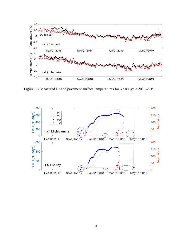
91
Figure 5.7 Measured air and pavement surface temperatures for Year Cycle 2018-2019

92
Figure 5.8 Measured FDs and TDs with FI/TI calculated using the pavement surface
temperature for Year Cycle 2017-2018. Data within circles will be excluded in the fitting
analysis
The measured FDs and TDs for the four sites for the two year cycles are shown in Figure 5.8
and Figure 5.9. FI and TI are also plotted, which are calculated starting from the first FD data
point with the pavement surface temperature using Eq. 3.1 and Eq. 3.2. At all the sites, FD takes
places around November 15th for each year cycle. The thawing season for the first year cycle is
earlier than that of the second year cycle. Because we can see that FD starts decreasing around
the beginning of March in Figure 5.8 but around the middle of March in Figure 5.9. This can also
be supported by TD prediction trends. TD continuously increases around the beginning of March
for the first year cycle but around the middle of March for the second year cycle. For all the sites
in Figure 5.8 and Figure 5.9, there are some data points marked with circles. This can be
explained in terms of two seasons. In the freezing season, several warm days may occur to thaw
the base and subgrade soils, as a result, FD decreases somewhat, especially at the beginning of
the freezing season. In the thawing season after the freeze-thaw cycle ends where FD meets TD,
there have some cold days to freeze the soils close to the base surface, leading to some FDs after
the freeze-thaw cycle ends.

93
Figure 5.9 Measured FDs and TDs with FI/TI calculated using the pavement surface temperature for
Year Cycle 2018-2019. Data within circles will be excluded in the fitting analysis

94
5.4.2 Application of Constrained Optimization for FD/TD Predictions
Predictions of FD and TD via constrained optimization for the two year cycles are shown in Figure
5.10 and Figure 5.11. In this constrained optimization, the circled data marked in Figure 5.8 and
Figure 5.9 are excluded. The major consideration is that these circled data appear either at the
beginning of the freezing season or after the thawing season due to the occurrence of some warm
and/or cold days. The primary aim of this study is to predict TD and FD trends in the thawing
season for accurately making SLR decisions. It is thus reasonable to exclude the circled data for
statistical analyses to obtain high prediction accuracy in the thawing season.
Figure 5.10 Predictions of FD and TD with the measured data for Year Cycle 2017-2018.
Circled data Fig. 7 are excluded

95
Figure 5.11 Predictions of FD and TD with the measured data for Year Cycle 2018-2019.
Circled data Fig. 8 are excluded
We can see in Figure 5.10 and Figure 5.11 that the predicted data for both FD and TD are in good
agreement with the measured data. In general, the predicted FD trends match well with the
measured FD trends, where FD increases in the freezing season and decreases when thawing starts.
Slight deviations for FD can be observed in Figure 5.11 in a few days at the beginning of the
freezing season because of the occurrence of some warm and/or cold days. This, however, has a
negligible effect because the predicted FDs in the thawing season, which are key for determining
the removal of SLR, are very close to the measured FDs. It is also seen that FD and/or TD is a
horizontal line after FD meets TD because imaginary numbers are obtained using Eq. 5.1 and Eq.
5.2. This, however, is not an issue because the freeze-thaw cycle ends already, thus, these FD
and/or TD values have no meaning.

96
Table 5.1 Fitting results for FD and TD
Site Year cycle Fitting constant for FD
a (cm oC-day-0.5) b (cm2 oC-day-1) c (cm2) d (cm) R2
Michigamme 2017-2018 7.9288 441.6752 43671.3354 233.9769 0.9454
2018-2019 7.3565 37.6986 5942.0144 102.1103 0.9826
Seney 2017-2018 9.5470 1129212.3434 55527423258.9767 235667.5752 0.9175
2018-2019 8.9973 66.8873 10452.0518 127.2441 0.9667
Eastport 2017-2018 12.2351 765988.3734 77196409094.8204 277867.4177 0.9695
2018-2019 10.5288 64.5584 14750.2992 146.4523 0.9738
Fife Lake 2017-2018 10.5395 77.0313 8406.6067 116.6875 0.9460
2018-2019 10.7898 35597.0232 23217827654.8394 152398.9745 0.9764
Fitting constant for TD
e (cm oC-day-0.5) f (cm2 oC-day-1) g (cm2) h (cm) R2
Michigamme 2017-2018 16.0829 1289.2506 63770.7833 227.5288 0.9337
2018-2019 0.0005 2234315.8950 448425887174.6080 669621.0911 0.9601
Seney 2017-2018 0.0000 437.2053 18992.6215 112.8137 0.9160
2018-2019 5.0099 583.8922 51533.6769 202.0103 0.9745
Eastport 2017-2018 10.7031 299.1526 19229.1109 113.6691 0.8085
2018-2019 0.6620 182.2324 25366.3592 134.2682 0.9651
Fife Lake 2017-2018 2.7082 1714226.7505 671747443635.2280 819577.0032 0.9212
2018-2019 5.0651 160.1695 26692.4104 138.3781 0.9777
The fitting constants for TD and FD are tabulated in Table 5.1. All the fitting constants are positive,
which satisfy the requirement of constrained optimization in Eq. 5.5. The determination coefficient
for almost all the predictions is found to be higher than 0.91, which further confirms the high
accuracy of predicting both FD and TD with constrained optimization. In Figure 5.10 and Figure
5.11, we also can see FD and TD are overlapped and equal to -25cm in the early freezing season
when no measured FD data point appears. This satisfies Eq. 5.6 for the physical meaning of the
fitting constants to reflect the pavement surface thickness. At the late stage of the thawing season,
FD meets TD in the predictions for all the sites, except Fife Lake in the second year cycle because
no more data is available after April 1st. However, it is expected that FD will meet TD later
according to their current prediction trends in Figure 5.11d.
Table 5.2 Site SLR determination

97
Site Year cycle Model determined date Suggested date
SLR on SLR off Duration (days) SLR off Duration (days)
Michigamme 2017-2018 2/27/2018 3/20/2018 22 4/2/2018 35
2018-2019 3/13/2019 4/1/2019 20 4/1/2019 20
Seney 2017-2018 2/24/2018 3/9/2018 17 3/16/2018 24
2018-2019 3/13/2019 3/25/2019 13 3/25/2019 13
Eastport 2017-2018 2/19/2018 3/1/2018 10 3/1/2018 10
2018-2019 3/15/2019 3/25/2019 11 3/25/2019 11
Fife Lake 2017-2018 2/19/2018 3/20/2018 29 4/8/2019 48
2018-2019 3/13/2019 - - - -
The FD/TD predictions in Figure 5.10 and Figure 5.11 can be used to determine the placement and
removal of SLR according to the suggested theory by Baïz et al. (2008) (see Figure 5.4). As shown
in Table 5.2, all the sites in the first year cycle have an earlier date for the SLR placement and a
later date for the SLR removal than the second year cycle. This is because the thawing season of
the first year cycle came earlier (see Figure 5.8 and Figure 5.9). The FD/TD model suggests that
the duration for SLR in Michigamme is 22 days for the first year cycle and 20 days for the second
year cycle, where these two numbers are very close. For the other three sites, the SLR duration of
the first year cycle is also close to that of the second year cycle. This implies that the SLR duration
in different years at the same site seems similar. Considering that there are a few warms and/or
cold days after FD meets TD when the freeze-thaw cycle ends (Figure 5.8), it is also suggested
that the removal of SLR can take place when no more TD data point appears to eliminate any
potential of thaw-weakening induced road damages. Such suggested dates for the SLR removal
are shown in Table 5.2 and we can see that the SLR duration of the first year cycle increases over
one or two weeks in Michigamme, Seney, and Fife Lake, while the SLR duration in Eastport keeps
unchanged.

98
5.5 Discussions
5.5.1 Advantages of Using Constrained Optimization for FD/TD Predictions
Constrained optimization has two major advantages that make it more advanced than non-
constrained optimization used in existing studies (Baïz et al. 2008; Bao et al. 2019) for statistical
analyses of the measured data. First, as clearly shown in Figure 5.10 and Figure 5.11, constrained
optimization can enable FD to meet TD in the thawing season. This can be further illustrated by
comparing FD and TD predictions with non-constrained and constrained optimizations. Figure
5.12 shows such a comparison for the statistical analyses of the data collected during 2017-2018
in Seney. We can see that FD cannot meet TD in the thawing season if non-constrained
optimization is employed, which has the same issue pointed out in Figure 5.1. However,
constrained optimization can resolve this issue to enable the prediction model to work in practice
in support of SLR decision-making.
Figure 5.12 Comparison of FD/TD predictions with non-constrained and constrained
optimization for Seney during 2017-2018
Second, when FI=TI=0 in the early freezing season, non-constrained optimization yields about -5
cm and 25 cm (Figure 5.12) for TD and FD, respectively. The two numbers are different and also
have a different sign simply resulting from the statistical analyses. They, however, cannot reflect

99
the realistic pavement FD and TD conditions. As explained in Section 5.3.2, these two number
should be equal because they represent the pavement surface thickness. It is clearly seen in Figure
5.12 that FD is equal to TD when constrained optimization is used. Therefore, constrained
optimization can yield not only satisfactory but more realistic results than those obtained with non-
constrained optimization.
5.5.2 Feasibility of Using Year Cycle 1 Fitting Constants to Predict Year Cycle 2 FD/TD
The FD/TD prediction model with constrained optimization can accurately predict the FD/TD
trends for applying SLR in each year cycle. It is also very interesting to explore the feasibility of
predicting the FD and TD trends in the current year cycle by directly employing the fitting
constants from the previous year cycle at the same site. This feasibility can further facilitate the
application of the prediction model in practice because it makes the model application more
convenient for road engineers for making SLR decisions without needing further measurements in
later year cycles.
To examine this feasibility, we predict the FD and TD trends during 2018-2019 in Michigamme
and Seney, respectively, using the fitting constants obtained during 2017-2018 from Table 5.1. As
shown in Figure 5.13, the predictions for both FD and TD lag behind and do not match the
measured data. The removal of SLR for Michigamme is determined on 3/21/2019, which is earlier
than the correct date of 4/1/2019. The SLR removal for Seney is also earlier and incorrect. The
major reason for causing the earlier predictions is that the thawing season during 2017-2018 is
earlier than that during 2018-2019 (see Figure 5.8 and Figure 5.9). Therefore, it is not feasible to
predict the FD and TD trends in the current year cycle using the fitting constants from the previous
year cycle. Though at the same site, the accuracy of the TD and FD predictions is also time-
dependent and significantly influenced by FI and TI accumulated during each year cycle.

100
Figure 5.13 Comparison of FD/TD predictions with non-constrained and constrained
optimization in Michigamme and Seney for Year Cycle 2017-2018
5.5.3 FD/TD Prediction Models are Better than a TI/FI Ratio for SLR Decision-Making
As mentioned in the introduction, a TI/FI ratio of 0.3 proposed by Mahoney et al. (1987) is still
used by several agencies in the U.S. to determine the removal date of SLR, e.g., those in
Washington (Mahoney et al. 1987; McBane and Hanek 1986). In this section, we evaluate the
accuracy of using this TI/FI ratio for SLR decision-making.
Table 5.3 shows TI/FI ratios calculated by TI and FI obtained on the SLR removal dates. The
removal dates are determined based upon the measured data in Figure 5.10 and Figure 5.11 when
FD either already or nearly meets TD. These dates can be considered as the true solutions for
removing SLR because the field measurements directly reflect pavement freezing and thawing
conditions. TI/FI ratios for Eastport and Fife Lake are not either fully or partially shown in Table
5.3. The reason is that the last FD and TD data points at these two sites in Figure 5.10 and Figure
5.11 are still far from each other; therefore, it is difficult to determine the correct SLR removal

101
dates. The SLR removal dates determined by the FD/TD prediction model are also presented for
comparison. We can see in Table 5.3 that the TI/FI ratios are not equal and/or very close to 0.3.
Even at the same site, the ratio is obviously different in two year cycles. This might be caused by
two possible reasons. First, FI and TI in Table 5.3 are calculated in terms of the pavement surface
temperature. This differs from the air temperature used in Mahoney et al. (1987) for obtaining a
TI/FI ratio of 0.3. Second, Mahoney et al. (1987) used “oF” for the temperature unit while “oC” is
utilized here.
Table 5.3 Ratios between TI and FI on the SLR removal date
Site Year circle FI (oC-day) TI (oC-day) TI/FI ratio SLR off
Measurement FD/TD model
Michigamme 2017-2018 737.68 47.64 0.06 3/19/2018 3/20/2018
2018-2019 843.32 106.13 0.13 4/1/2019 4/1/2019
Seney 2017-2018 561.87 43.46 0.08 3/6/2018 3/9/2018
2018-2019 638.67 87.14 0.14 3/25/2019 3/25/2019
Eastport 2017-2018 334.25 65.38 0.20 2/28/2018 3/1/2018
2018-2019 - - - - 3/25/2019
Fife Lake 2017-2018 - - - - 3/20/2018
2018-2019 - - - - -
To further examine the accuracy of using the TI/FI ratio, we calculate the TI/FI ratios for three
additional sites of Mackinac Bridge, US-10, and US-12 in the Superior region in Michigan (see
Figure 5.2). In the calculation, we adopt the air temperature to compute FI and TI using both “oF”
and “oC” temperature units. The removal dates of SLR are determined based upon the field
measurements when FD meets TD. It is clearly seen in Figure 5.4 that the TI/FI ratio is not equal
to 0.3, no matter “oF” or “oC” is utilized. The TI/FI ratio is in a range of 0.26-2.37 when “oF” is
used.
Table 5.4 SLR removal dates at three additional sites in the Superior region in Michigan
Site Year Date SLR off FI TI TI/FI ratio
oF-day oC-day oF-day oC-day if oF if oC
Mackinac Bridge 2017 4/5/2017 694.00 477.22 362.00 201.33 0.52 0.42
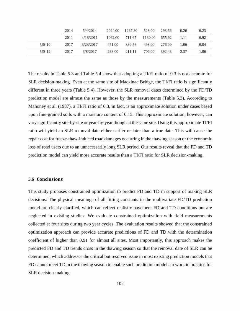
102
2014 5/4/2014 2024.00 1267.80 528.00 293.56 0.26 0.23
2011 4/18/2011 1062.00 711.67 1180.00 655.92 1.11 0.92
US-10 2017 3/23/2017 471.00 330.56 498.00 276.90 1.06 0.84
US-12 2017 3/8/2017 298.00 211.11 706.00 392.48 2.37 1.86
The results in Table 5.3 and Table 5.4 show that adopting a TI/FI ratio of 0.3 is not accurate for
SLR decision-making. Even at the same site of Mackinac Bridge, the TI/FI ratio is significantly
different in three years (Table 5.4). However, the SLR removal dates determined by the FD/TD
prediction model are almost the same as those by the measurements (Table 5.3). According to
Mahoney et al. (1987), a TI/FI ratio of 0.3, in fact, is an approximate solution under cases based
upon fine-grained soils with a moisture content of 0.15. This approximate solution, however, can
vary significantly site-by-site or year-by-year though at the same site. Using this approximate TI/FI
ratio will yield an SLR removal date either earlier or later than a true date. This will cause the
repair cost for freeze-thaw-induced road damages occurring in the thawing season or the economic
loss of road users due to an unnecessarily long SLR period. Our results reveal that the FD and TD
prediction model can yield more accurate results than a TI/FI ratio for SLR decision-making.
5.6 Conclusions
This study proposes constrained optimization to predict FD and TD in support of making SLR
decisions. The physical meanings of all fitting constants in the multivariate FD/TD prediction
model are clearly clarified, which can reflect realistic pavement FD and TD conditions but are
neglected in existing studies. We evaluate constrained optimization with field measurements
collected at four sites during two year cycles. The evaluation results showed that the constrained
optimization approach can provide accurate predictions of FD and TD with the determination
coefficient of higher than 0.91 for almost all sites. Most importantly, this approach makes the
predicted FD and TD trends cross in the thawing season so that the removal date of SLR can be
determined, which addresses the critical but resolved issue in most existing prediction models that
FD cannot meet TD in the thawing season to enable such prediction models to work in practice for
SLR decision-making.

103
From the discussion, we confirmed that it is not feasible to predict the FD and TD trends in the
current year cycle by directly employing the fitting constants from the previous year cycle at the
same site. Our results also revealed that the FD and TD prediction model is more accurate for SLR
decision-making than a TI/FI ratio of 0.3 that still has been used in several agencies in the U.S.
The TI/FI ratio can vary significantly site-by-site or year-by-year though at the same site.
Therefore, the FD and TD prediction model with constrained optimization reported in this study
is reliable and highly recommended for making SLR decisions for roadways in cold regions.

104
Chapter 6 Development of Web-Based Spring Load Restriction Decision
Support Tool
6.1 Abstract
Thaw-weakening is a major cause of pavement damage in seasonally-frozen areas covering half
of the U.S., leading to huge financial costs for taxpayers. In recent years, the damage has lessened
due to improving practice with Spring Load Restriction (SLR) policies. However, even the most
advanced SLR date prediction methods/tools are still primitive from the perspective of information
technology. Such methods/tools are obtained and/or implemented manually with a small amount
of data or even directly based on experience. The chapter reports what has been learned from an
ongoing project supported by the Michigan Department of Transportation for the development of
a web-based SLR decision support tool, i.e., a web-based app called MDOTSLR. MDOTSLR
provides the access to much more data with little latency and automates data acquisition,
processing, and decision making. In this chapter, the models and data supporting the functions of
the tool will be first introduced. Next, the major functions (or services) of the app will be detailed.
Followed will be the software engineering details for the development of the app. Compared with
traditional tools without web delivery, this web-based tool automates the acquisition and
processing of weather data, GIS data, and road weather information in real time and thus enables
more accurate and convenient SLR predictions. In the accomplished automatic mode, no labor is
required to keep the data up to date. The tool can be easily extended or modified for most state
DOTs for immediate financial savings in road maintenance and less disturbance to the local
economy.
The main purpose of this chapter is to detail the development of a web-based tool that uses the
freeze-thaw model for assisting in SLR decision making to allow MDOT, local road agencies, and
road users to better predict the dates for SLR placement and lifting. The web-based tool we are
developing is accessible from any electronic device with Internet access and a web browser, which
will be more convenient for users. Compared with traditional tools without web-based delivery the
web-based tool we are developing can collect the data more timely and more comprehensively, as
it can always acquire the latest data, including the weather data, Geographic Information System
(GIS) data, and Road Weather Information Station (RWIS) data.

105
The remainder of the chapter is arranged as follows. First, an overview of the development goals
for the web-based tool is presented. Then, the models and data employed for the web-based tool
are introduced. This is followed by an explanation of the organization and functionality of the web-
based SLR decision support tool that we have already developed. Next, software engineering
details, especially the two major services in the app, will be given. Finally, conclusions are drawn
as a summary of the whole chapter.
6.2 Goals for the App Development
6.2.1 Objectives
The objective of the project MDOT OR 16-009 is to establish how the web-based tool for setting
and removing Seasonal Load Restrictions (SLR) will be set up as its development continues. The
desired end state is a tool which will give industries the most amount of time to prepare for the
restrictions and minimize the time to lift the restrictions. To be specific, recommendations will be
made for the users of the tool to predict the accurate time to post and remove SLR signs so that the
pavement structures can be protected from excessive damage during the spring thaw season and
hauling industries can minimize losses. In addition, a user-friendly decision support tool is being
developed, which will provide all the relevant data used by the recommendation algorithm to the
user. This way the data could be easily utilized by the public and private sector in estimating
potential thaw conditions using their own methods and in developing their own models for SLR.
The work that has been accomplished has produced a tool called MDOTSLR at mdotslr.org.
6.2.2 Features and Benefits
This tool can not only be applied in Michigan but also other states in the U.S. Minnesota DOT
(MnDOT) once published a web-based tool similar to ours. However, MnDOT’s tool divides
Minnesota into only 4 parts to help make the SLR decision, which is far less precise than the web-
based tool that we are developing. Also, MnDOT’s tool mostly relies on air temperature for
predictions while there is not GIS and RWIS data for predictions or validations.

106
In our web-based tool, the users can retrieve the information of every specific district by inputting
a zip code. For instance, if a user enters a zip code of 49931, then all the information for Houghton,
MI, will be presented to the user. In addition to Michigan zip codes, the tool also supports
Wisconsin and Minnesota zip codes. Furthermore, MDOTSLR will be able to provide a prolonged
prediction, i.e., one month, which is much longer than that can be offered in the other existing
tools, though as of now it only supports ten-day predictions. This will give users more time to
prepare, with the caveat that weather forecasts are always associated with uncertainties that
increase with time; a prediction for a time far from now is associated with more uncertainties. In
addition, many more services are provided in the web-based tool we are developing than the one
developed by MnDOT. Finally, MDOTSLR uses a variety of data types rather than merely air
temperature. Function details in methods, data, and functions will be provided in later sections.
Compared with traditional non-web SLR decision support tools, the web-based tool we are
developing has a series of benefits:
❖ A powerful tool for SLR practice is provided for the MDOT, local road agencies, and
public road users in Michigan, currently based on freezing/thawing index values.
❖ MDOT and local road agencies can better determine the dates for placing the removing the
SLR with this tool. The tool can provide the users with a much more accurate, convenient, and
automated SLR decisions, which can effectively save the investment in repairing the road damage
induced during the spring thaw season and effectively prolong the service life of the pavement.
❖ Since this process is automated, less labor would be required for determining SLR since
all a road engineer has to do is quickly validate the data instead of doing all the calculations
themselves.
❖ The road users, especially those seriously affected by the SLR policy, such as trucking
companies and industries that rely on hauling services will also benefit from this tool. More time,
in fact, much more than other states, i.e. one month instead of several days, will be given by the
tool, once the forecast range is increased, for the users to prepare for the SLR placement or
removal. Both the road users and the economy of Michigan will benefit a lot from this tool.
❖ The tool will change the current practice in Michigan and make the SLR practice better
guided by scientific and engineering principles and benefit from the digital infrastructure, which
will enhance the current web services provided by MDOT.

107
❖ This tool will also provide suggestions and information for future RWIS sites and help
refine the pavement design so that it can better consider frost effects.
❖ This tool can be easily extended or modified for most states in the U.S. as well as other
places around the world. Its use could lead to an incalculable save in the budget of state DOTs,
local road agencies, and road users.
6.3 Models and Data
6.3.1 Models
Seasonal Load Restrictions have been used for a long time. In the past, traditional methods usually
rely on engineers’ experience and visual observations in situ. For example, in Michigan, as
described on the CRA website, the road commissions employ licensed Professional Engineers to
make these decisions and also consult neighboring road agencies.
Despite the historical statistics, more and more agencies are turning to use quantitative SLR
decision algorithms. After a lot of efforts, several popular methods have been produced to
determine the placement and removal dates or the duration of the SLR.
Previous analytical models often use the parameters including air freezing, thawing indices and
cumulative thawing index (CTI) and so on, to determine the SLR application and removal dates.
The current version of the tool uses these models to recommend SLR. However, it has been found
that the predictions of freezing and thawing depths, especially the latter one, are the key to better
determine the placement and removal dates of SLR, as the depth and thickness of the frost in the
pavement determine the seasonal fluctuations in the bearing capacity of the road.

108
Figure 6.1 SLR decisions with freezing/thawing depth predictions (Baïz et al. 2008)
The correlation between freezing/thawing depths and the spring thaw period has been studied. As
illustrated in Figure 6.1, the time for SLR placement corresponds to the time when the continuous
thawing starts in the subgrade soils. After the thawing depth (moving downward) meets the frost
depth (moving upward) in the thaw season, SLR should be removed.
Accurate SLR decisions made using the predictions of freezing/thawing depths are highly
desirable. This is because most agencies are required to notify the public of SLR postings at least
3 to 5 days in advance. Therefore, the freezing/thawing depth predictions already available in the
depth-curve service will be implemented in the SLR recommendation service which will allow for
this advanced notice. Note that either extensive damage to the pavement owing to late placement
or early removal of the SLR, or economic loss of road users due to an unnecessarily long period
for SLR will be caused by the inaccurate predictions of these depths.
There are several different types of procedures (methods or criteria) for SLR decision making
based on freezing/thawing depth predictions. These include the Mahoney et al. (1986) model
(Mahoney et al. 1987) for WSDOT and FHWA, the Berg model (Berg et al. 2006) for the US
Forest Service which was initially used by the NH DOT, the MnDOT Models (Van Deusen et al.
1998), and the MIT method (Manitoba Department of Infrastructure and Transportation, (Bradley
et al. 2012)). Although these models were developed based on field experience and long-term
observations and have been tested by for years, they cannot be directly applied to Michigan due to

109
different weather, soil, and pavement conditions. Therefore, new models which have been adjusted
with Michigan-specific data are used in this web-based tool. The models are generated with RWIS-
site-specific data via multivariate statistical analysis using the following two equations. For the
predictions of SLR dates, we currently adopted the FHWA model. However, we will make the
predictions site-specific in the next stage.
𝐹𝐷 = 𝑎√𝐹𝐼 + √𝑐 − 𝑏𝑇𝐼 + 𝑑 Eq. 6.1
where a, b, c, and d are fitting constants, the first three always positive. Mainstream viewpoint is
that freezing and thawing have similar processes, thus the mathematical formulation for TD and
FD are similar:
𝑇𝐷 = −𝑒√𝐹𝐼𝑇 − √𝑔 − 𝑓𝑇𝐼 + ℎ Eq. 6.2
where e, g, f, and h are fitting constants, in which the first three always positive. 𝐹𝐼𝑇 is the
cumulative freezing index in the thawing period only.
6.3.2 Composite Data Mapping Service
Composite data refers to all three categories of data being displayed for one geographical area, in
the case of mdotslr.org/services/data-map points are used. The purpose of this service is to provide
the composite data of each RWIS station, that is RWIS, soil and weather data at the geographical
coordinates of each station. The current limitation of the RWIS data is a small number of data
points. Without interpolation, we only have one hundred and five data points to work with whereas
the weather and soil data span the state. Until a good method of interpolation is put into place we
are limited to these points. The method used to map the RWIS stations to a zip code and map unit
is as follows: make a call to the google maps API to get the zip code and county for the station.
Since we have the zip code right off the bat that mapping is done. As for the county, each legend
area, larger areas that contain individual map units, happens to be broken down by county with a
few exceptions that were controlled for. We take the county name and make a call to the soil
database for all map units and their geographical polygons in that legend area and then check each
polygon using a point in polygon algorithm, provided by the turf.js library, to find which map unit

110
the station is in. We then save the map unit and zip code as properties of the station in the database
so we do not have to do another time-consuming search for it when we actually pull the data. This
process worked for all but two of the RWIS stations. Further investigation would be needed to
figure out why but it would be much faster to find these two stations map units visually, show the
stations and show the possible map units on an actual map and then pick and save the correct map
unit. This is on the to-do list. Since each RWIS station is mapped to a map unit and a zip code all
we have to do is make calls for their data and we can quickly provide the composite data to the
users of the website. The front end formatting of the table is somewhat trivial, though time-
consuming to set up, and to some extent arbitrary so we will omit that part of the service.
6.3.3 Optimization of MongoDB Queries
The MongoDB queries were sped up using the standard practice of only selecting relevant data
from the database. This seems obvious since we do not want to waste time pulling information
from the database we do not need but it was not intuitive. By default, when you make a MongoDB
query it pulls the entire object of each record but you can select just the fields you want by passing
the names of these fields to the query call. It gets slightly more complicated when dealing with
relational information but for the most part uses the same process. We had not learned about this
method until recently since all our previous projects were small proof of concept stuff that did not
deal with huge amounts of data but at least we are now running at the proper speed. Extra care
should be taken in the future by anyone contributing to the project to read and understand how to
make these selective queries in order to keep all future services running fast.
6.4 Functions and Organization of the APP
The tool aims to provide two modes for users: automatic and manual. In the automatic mode, the
users do not need to provide input and they can receive an estimate based on the default values. In
the manual mode, users can input site-specific information such as the pavement type for a better
prediction. As of now, the automatic mode has been finished while the manual mode is still under
development.

111
As shown in Figure 6.2, our web-based tool has four main services, including 1. Temperature, F/T
indices & SLR prediction, 2. Map of freezing/thawing indices & RWIS station, 3.
Freezing/thawing depth by ZIP code, and 4. Freezing/thawing depth by RWIS station.
Figure 6.2 Homepage of MDOT SLR App
Figure 6.3 Page of temperature, F/T indices & SLR prediction
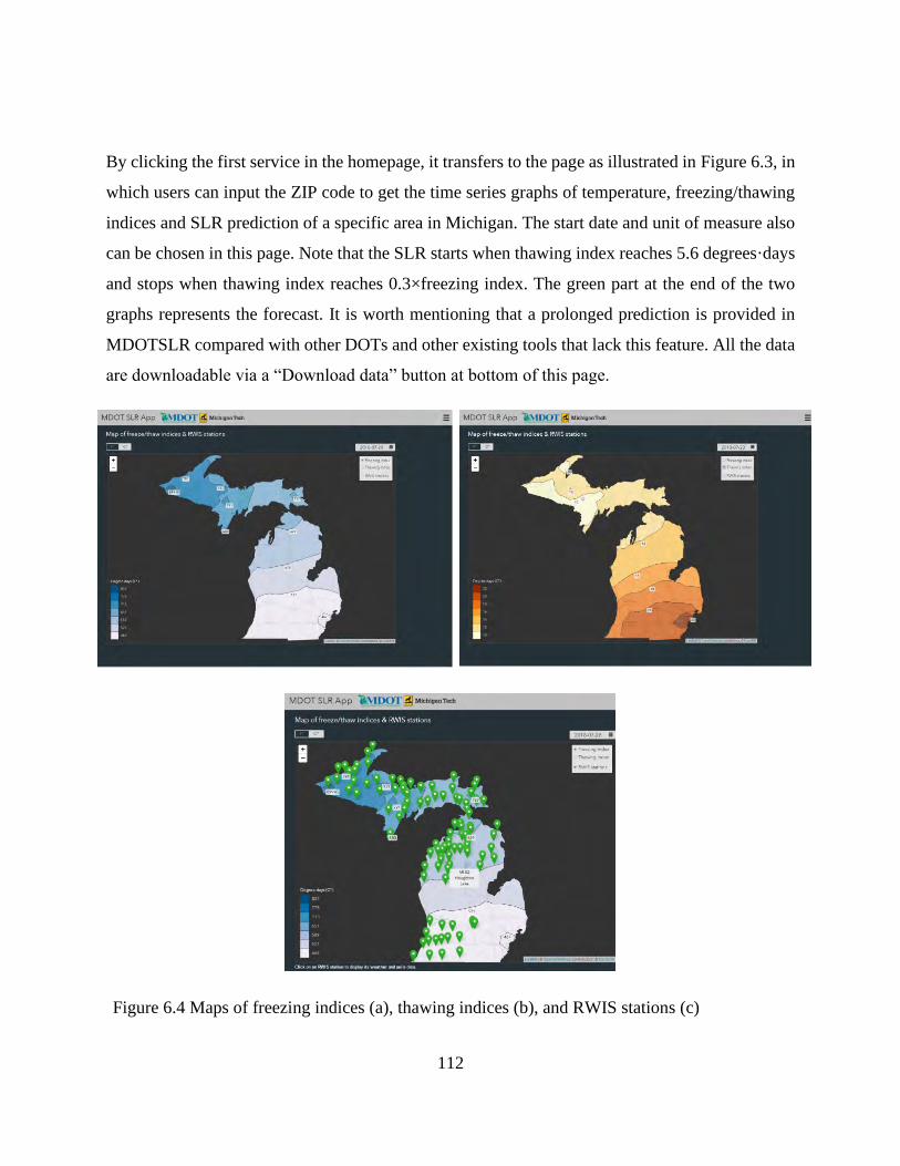
112
By clicking the first service in the homepage, it transfers to the page as illustrated in Figure 6.3, in
which users can input the ZIP code to get the time series graphs of temperature, freezing/thawing
indices and SLR prediction of a specific area in Michigan. The start date and unit of measure also
can be chosen in this page. Note that the SLR starts when thawing index reaches 5.6 degrees·days
and stops when thawing index reaches 0.3×freezing index. The green part at the end of the two
graphs represents the forecast. It is worth mentioning that a prolonged prediction is provided in
MDOTSLR compared with other DOTs and other existing tools that lack this feature. All the data
are downloadable via a “Download data” button at bottom of this page.
Figure 6.4 Maps of freezing indices (a), thawing indices (b), and RWIS stations (c)

113
In the second service, a map of freezing/thawing indices and all three categories of data, i.e.,
weather, GIS, and RWIS, which are indexed using RWIS sites, are provided. Users can choose to
see the freezing/thawing index contour lines intuitively from this map (Figure 6.4a and Figure
6.4b). Additionally, all the RWIS stations for Michigan are presented in the map (Figure 6.4c),
thus the users can view the soil data and daily weather data of each station by clicking a green
marker which represents a station on the map.

114
Figure 6.5 SSURGO soil data of the selected station (a) and daily weather data of the selected
station (b)
For example, if the user clicks the green marker which represents the MI-02 Houghton Lake as
shown in Figure 6.4c, the information of this station will be displayed as shown in Figure 6.5.
Figure 6.5a shows a table of SSURGO soil data including the layer, clay total, sand total, silt total
and water content. Users can also find a table of daily weather and RWIS data as shown in Figure
6.5b, which includes the parameters of average humidity, average temperature, average visibility,
max wind speed, total precipitation, maximum air temperature, minimum air temperature, base
temperatures at different depths, and chemical factor and so on.
Figure 6.6 Predicted variation of freezing/thawing depth
The third main function of MDOTSLR (Figure 6.6) is that the users can view the time series graph
of freezing/thawing depths of a specific area once they select a ZIP code. The start date and units
can be assigned as well.

115
Figure 6.7 Measured variation of freezing/thawing depth
In the last service, users can view the time series graph of freezing/thawing depth for a selected
RWIS station (see Figure 6.7). Note that the same depth calculations are used in this part as for the
ZIP code-based depth, however, the underground RWIS sensors are used to calculate the depth
rather than the surface air temperatures. As mentioned before, there is a difference between the air
temperature and the pavement surface temperature, so that they are taken into consideration
respectively.
6.5 Construction of the App
6.5.1 Data Transfer and Workflow
In the default automatic mode, the users just need to enter the zip code for the area of interest to
obtain the temperature and SLR predictions, freezing/thawing depth predictions, and measured
freezing/thawing depth. With further development, the users will also be able to draw a line (either
straight line or polyline) or click one point in a map on a web page to select a road or road segment

116
that he/she is interested in. As shown in Figure 6.8, the request from the user is be sent to the server
and translated into accurate location information. The main program on the server will then request
weather and GIS information from NOAA/Accuweather and WebSoilSurvey/GeoWebFace. This
information will be used to calculate the freezing/thawing depth as well as the SLR
recommendations. Both the freezing/thawing depths and SLR recommendations will be sent back
to the front-end, that is, the user’s electronic device. The web browser on the user’s side will
process the data and show predicted freezing and thawing depths vs. location lines for the next 30
days. A potential SLR placing or lifting sign will be shown if it is predicted as possible (should or
must level) during the time range. Given the current progress made, once extrapolation of the
RWIS data has been completed, this functionality will be easy to implement since we already have
the work for setting up and taking input from the map taken care of.
Figure 6.8 The calculation framework of the web-based tool
6.5.2 Development of the Web-Based App
The web-based app is essentially a dynamic website. For the front-end design, the web pages are
written using HTML5 and CSS3 compiled from SASS. The responsive web design approach is
adopted to make sure the website can be optimally accessed with all major types of electronic
devices, i.e., desktops, tablets, and mobile phones. jQuery, a JavaScript library, is used to enhance
the functionality and user-friendliness of the front-end pages. The mapping and location fetching
are achieved with OpenStreetMap and Leaflet.js. Data transfer between the front-end and the
server is conducted via JSON. Nodejs (a JavaScript-based programming platform) is used to

117
manage the retrieval of data from the weather and RWIS sites while MongoDB (a noSQL database
technology) is used to store the data locally. Though SQL has traditionally been used as the go-to
database for web app’s, MongoDB was used for its high speed and ease of use. Even though
MongoDB is not fully atomic, meaning all documents are protected in case one query fails, this is
not an issue since queries are almost always read-only, with the exception of the automatic data
retrieval that occurs once a day. For serving the app, Express, a Node.js website framework, is
used to deliver HTML documents and the actual data earlier detailed. The calculation process is
programmed on the server side using Node.js to shorten the development cycle, though the
calculations were developed using separate technologies. Weather and GIS information is obtained
via APIs made available from the sources listed previously. The calculation results are shown as
charts and tables on the web pages. This plotting functionality is developed using the free software
charting library, Chart.js.
6.5.3 Freezing/Thawing Index Acquisition on Backend
Every service of the app uses a number of different data sources from the database, each doing
their assigned job but the easiest place to start in this process would be the data routes as that is
where the data is pulled in from MongoDB, processed and then sent off to the client. All data
served by the app is served from a subroute of https://mdotslr.org/data, though only its subroutes
actually serve data, i.e., https://mdotslr.org/data/tempCurve/49931, serves the temperature and
freezing/thawing index data for Houghton. Though the data is only one portion of the app, it serves
as a good starting point as each data sub route relates directly to one of the services.
The temperature curve data route, https://mdotslr.org/data/tempCurve/, is the first sub route and
serves data to the first service developed last quarter (https://mdotslr.org/services/temp-curve),
though many changes have been made this quarter including the addition of two new states weather
data, Minnesota and Wisconsin. The route takes a zip code in a GET request and returns the
temperature, freezing/thawing index and SLR recommendations in JSON format. Thus, for the
link https://mdotslr.org/data/tempCurve/49931, the zip code we are selecting is 49931 and the data
returned will be for that zip code.

118
The first step is to retrieve the past and forecasted average temperature from MongoDB and the
wunderground API respectively. This is done through a query to the database which returns the
past data and another HTTP GET request made by the server to the wunderground API which
returns the forecasted data. Both of these requests are handled asynchronously meaning we make
a request for this data without blocking the thread our server runs on. This is the default behavior
of Node.js and this non-blocking paradigm allows us to handle multiple requests and calculations
pseudo-concurrently as opposed to sequentially, which makes serving data to multiple users at the
same time much faster.
The data is stored on the server in a JSON-like format, which makes it very straightforward for
Node.js to handle and for express to send to the client. The JSON format is predefined in a model
so we know exactly what fields we have to work with, in this case, we are just using the average
temperature of each day but other data fields are available. The data that comes in from the
wunderground API is also in JSON format and is organized very similarly to our data, so joining
the two together is simple.
With that, we have all the past weather data and the next 10 days forecast. Originally the plan was
to also store the 10-day forecast into the database but since the forecast is likely to change it was
changed to make live API calls at each request. With that, we have all of our average temperature
data that would be returned to the client. Returning the data to the client is handled by Express
which simply takes our JSON and sends it off.
However, before the request is returned we must use the temperature data to calculate our freezing
and thawing indices and include that in our response to the client.
In short, the function that calculates the freezing index follows this equation:
Eq. 6.3
and the thawing index is calculated using the following equation:
Eq. 6.4

119
With the difference being the app does this all in JavaScript as opposed to mathematical notation
so the actual code and process are slightly different.
For these equations, i represents the current day in the sigma equation, or in JavaScript the current
iteration of the loop that processes each day, and N is the total number of days in the collection. Ti
is the average temperature of the current day being iterated through, and Tref is the offset used to
account for the temperature difference between the pavement in the air, though it is not 100%
successful and this discrepancy is the main flaw in this model. Using these equations, the freezing
and thawing indices are calculated, and each step of the summation is also saved so we can show
the changes over time where:
FIi = ∑ (0 − 𝑇𝑗)𝑖𝑗=1 Eq. 6.5
and
TIi=∑ (𝑇𝑗 − 𝑇𝑟𝑒𝑓)𝑖𝑗=1 Eq. 6.6
which gives us the indices for each day as well as the final day.
During this summation, or looping through the data, we also mark which dates, or which i, should
be the start and end of SLR. If TIi > 5.6, we mark i as an SLR start date or if SLRs have already
started, a continuation of the SLR period. If TIi >= 0.3 * FIi, we mark i as and SLR end date. In
addition to these calculations, there are also some simple fuzzy rules for determining when the
freeze-thaw cycle is and when to reset the values for a new freeze-thaw cycle. Since we’re using
a programming language and not just doing each of these calculations separately, all of these
calculations and the SLR classification can be done in O(N) operations, N being our total number
of days in the collection. With the calculations are finished, the data is sent off to the front end by
Express to be graphed by the client.
6.5.4 Freezing/Thawing Depth Acquisition on Backend
The other main service of the app is the RWIS based freezing and thawing depth calculator, found
at https://mdotslr.org/services/road-depth-curve. It uses RWIS data provided by the Vaisala API

120
to calculate the freezing and thawing depth using underground temperature sensors. The
temperature data is reported from several RWIS stations set up throughout Michigan that have
these sensors installed. Just like with the last service, the data returned from this API is stored
locally in MongoDB, organized by each station's unique id in the database. Getting back to the sub
route itself, this service starts at the https://mdotslr.org/data/stations data route. Unlike the freezing
and thawing indices service, this service uses a drop-down menu to select the station you want to
see the data for. When you select a station from the drop down, an addition GET request is made
via jQuery’s ajax function to our sub route, i.e., https://mdotslr.org/data/roadIndices/11760 where
11760 is a unique station id.
Once the data request has been made to the server, Node.js retrieves the underground temperature
data for every day recorded from MongoDB. Each day returned follows a set format, just like with
the weather data, where the multiple sensors that each RWIS station reports are organized in JSON
format. This data route is only concerned with the underground temperature data for each day since
we are trying to determine the freezing/thawing depth, so that is the only field retrieved from
MongoDB.
With the temperature data retrieved, we use it to determine the freezing and thawing depth either
by direct observation or by interpolation. We are essentially working with a tuple of tuples that
hold depth, temperature pairs:
[[D1,T1], [D2,T2], … [DN,TN]]
where N is the total number of sensors. Each sensor is ordered by the depth, so the interpolation is
fairly straightforward. We just need to iterate over each sensor and apply the following rules:
if Ti = 0
if F is not set, F = Di
else, T = F and F = Di
else if 0 is between Ti and Ti - 1
if F is not set, F = interpolated depth between Di and Di - 1

121
else, T = F and F = interpolated depth between Di and Di – 1
where,
Di = current iteration depth
Di - 1 = last iteration depth
Ti = current iteration temperature
Ti - 1 = last iteration temperature
F = freezing depth
T = thawing depth
Using these rules as we iterate through each tuple, we are looking for the freezing point, or where
the sensors report 0 degrees Celsius. This depth is either a freezing depth or a thawing depth. If
the sensors don’t directly report where 0 is, we need to use linear interpolation to determine where
0 lies between two sensors. This interpolation is done using the following equation:
Dint = ( 0 - Ti - 1 )×( Di - Di - 1 ) / ( Ti - Ti - 1 ) + Di - 1 (7)
The above equation is just a standard linear interpolation. The reason we set F and then switch it
out if a new 0 point is found is that we assume that for two 0 points, the one occurring higher in
the soil, or for lower Di values, is the thawing depth since thawing occurs faster from the surface
downwards than from the subgrade upwards.

122
Figure 6.9 Variation of freezing and thawing depth with time
As shown in Figure 6.9, this same process is repeated for every day in our collection of days and
the freezing/thawing depths are stored in their own collection of days which we return to the client
using Express where it is graphed. For one station the calculation process takes O(D*N) where D
is the number of days in the collection and N is the number of depth sensors the station has.
6.5.5 Refactoring
In early versions of the app, the entire project was written using callback functions. Callback
functions refer to the fact that certain resources, pulling data from a website or making a database
call, don’t take a predictable amount of time. We call this asynchronous programming, async for
short, were not all of the code is run in the order written. One way to deal with this is to pass
callback functions to the resource you’re pulling from. When the resource is ready it fills your
callback function with the data you requested and execution of the script can continue. The only
problem with this is that every time you write a function you have to indent the file and after
passing upwards of 3 callback functions the code starts to get hard to follow and code that’s hard
to follow is hard to maintain. To combat this problem, Javascript has special functions called async
functions that return a Promise object. Async functions have special rules that let them pause
execution to wait for a resource using the await keyword. This means async code can be written

123
all within the same indent making everything look nice and easy to understand. With all that in
mind, we recently went back and refactored much of the code to implement async functions. The
hope is that since the code isn’t a huge indented mess anymore it will be easier to work on and
updates can be made faster.

124
Figure 6.10 The first picture shows the re-factored code, it is all on one indent and uses await
calls instead of callbacks
6.5.6 Map Binary Search
This section presents the effort that we made to address the challenge to map the GIS data from
the websoilsurvey to any location associated with a zip code, county, or RWIS site. To start we
have a map full of zip codes and map units, for the sake of this example we have only illustrated
one of each but in reality there would be many.
Figure 6.11 Schematic of map binary search: original map
We start with a box around the entirety of Michigan, working with one peninsula at a time. We
then divide the box in two over and over until the box is small enough to only be in one map unit
and one zip code.

125
Figure 6.12 Schematic of map binary search: one box
We have only illustrated one divide but in reality every box would continue to make divides until
they are in the same state as the one illustrated. This chain of divides is saved to the database. Now
when we have a point we want to find:
Figure 6.13 Schematic of map binary search: refined boxes
We can keep track of the divides we made and use that to identify which box the point belongs in
and in turn which map unit and zip code the point has. There will be an enormous number of divide

126
chains saved to the database but they can be encoded very efficiently as binary data. We can
represent each new box as either a one or a zero, zero for the first box made by the divide and one
for the other. This binary data will be very small so storage shouldn’t get too large. Another
advantage of this method is that the point in polygon algorithm is extremely efficient for rectangles.
So the loading time, in theory, should be short.
6.6 Conclusions
The development progress and future development plans for the MDOT web-based SLR prediction
tool, i.e., MDOTSLR, have been detailed in this chapter. This tool is for the benefit of MDOT,
road agencies, and road users since they will be able to make better decisions about when SLR
should be started and ended. Freezing/thawing depth prediction models, which are considered a
key factor to the prediction of SLR, will be used by this tool to provide more accurate results and
will replace the current freezing/thawing indices model in place now. RWIS information,
significant Weather, and GIS soil data are automatically collected by MDOTSLR to make SLR
decisions with plans to expand the current database to include solar radiation data and a longer
date range of all data types.
To conclude, the web-based tool we developed has functions and advantages as follow:
❖ Automatic SLR prediction accompanied by the data used to predict SLR so users may
calculate it manually with a different model or develop their own models from the data.
❖ Searching by ZIP code, the users can get the time series graphs of average temperature,
freezing/thawing index and SLR prediction.
❖ Users can view freezing/thawing index contour lines for any date as well as RWIS stations
on the map of Michigan. By clicking on an RWIS station, the users can get the information
of soils and daily weather. (https://mdotslr.org/services/map)
❖ Both searching by the ZIP code and RWIS station, the users can get the time series graphs
of the freezing/thawing depth. Note that the freezing/thawing depth by ZIP code is
calculated by the air temperature (https://mdotslr.org/services/depth-curve) while the
freezing/thawing depth by RWIS station is calculated by the pavement surface temperature
(https://mdotslr.org/services/road-depth-curve).

127
❖ Compared with other existing tools, the web-based tool we developed is more accurate,
convenient, user-friendly, automatic and feature rich. With the implementation of a longer
forecast, it will provide a much longer prediction than other tools.
❖ The tool will significantly enhance the current web services provided by MDOT. Studies
that use the tool as a resource will help refine the pavement design to better consider frost
effects and provide suggestions and information for future RWIS sites.

128
Appendix
FD/TD Prediction Models Obtained with RWIS Data 2017-2018
Important
Notes
Note A
Fitting function for
FD: FD=a*FI^0.2+(c-b*TI)^0.5-d
Fitting function for
TD: TD=-e*FIT^0.5-(g-f*TI)^0.5+h
Fitting constraints FD: c^0.5-d=0.25 TD: -g^0.5+h=0.25
Measured situation 1: depth=[0;3;6;9;12;18;24;30;36;42;48;54;60;66;72]
Measured
situation 1
Site Fitting parameter Fitting constant
FD a (TD
e) FD b (TD f) FD c (TD g) FD d (TD h) r^2
Charlevoix FD with freezing cycle 10.46 3398479.01 8329021367327.90 2886029.39 0.96
TD with thawing cycle 12.62 6729249.71 9098417670462.76 3016333.35 0.46
Glennie FD with freezing cycle 9.01 1049235.17 1027864588018.50 1013861.57 0.76
TD with thawing cycle 38.93 1798820.29 239192937999.03 489048.55 0.86
Cadillac South FD with freezing cycle 4.29 28087.87 5140425402.13 71721.76 0.86
TD with thawing cycle 0.00 349807.28 239137715029.24 488992.09 0.66
Eastport FD with freezing cycle 12.16 521.44 44940.40 236.99 0.97
TD with thawing cycle 10.70 299.15 19229.11 113.67 0.81
Fife Lake FD with freezing cycle 10.79 1511.04 1309376.37 1169.29 0.93
TD with thawing cycle 36.87 6831142.56 5351199864511.11 2313241.07 0.57
Wolverine FD with freezing cycle 12.74 1927272.28 147084221172.63 383540.61 0.43
TD with thawing cycle 27.06 606.17 40378.04 175.94 0.72
Williamsburg FD with freezing cycle 5.02 75.74 4706.63 93.60 0.74
TD with thawing cycle Only 1 data point
West Branch FD with freezing cycle 8.91 2302.26 318871.91 589.69 0.96
TD with thawing cycle 0.32 349.50 13208.83 89.93 0.96
Wellston FD with freezing cycle Need TD data to calcualte TI

129
TD with thawing cycle No data point
Waters FD with freezing cycle 8.26 38.59 5909.32 101.87 0.96
TD with thawing cycle 2.62E+00 16841557.51 214932656724285.00 14660561.84 0.51
Walloon Lake FD with freezing cycle 5.65 91241.80 24908181751.87 157848.26 0.89
TD with thawing cycle 0.00 242716.56 146353610036.38 382536.90 0.50
Sherman FD with freezing cycle 5.73 458458.28 274551215053.46 524001.35 0.92
TD with thawing cycle 0.13 1428859.23 1159236899600.87 1076653.64 0.70
Rose City FD with freezing cycle 5.45 175708.69 50301126130.76 224304.13 0.32
TD with thawing cycle 0.00E+00 8.03E+04 13470726159.78 116038.46
2.60E-
02
Presque Isle FD with freezing cycle 8.59 530014.81 27174946019.24 164873.25 0.82
TD with thawing cycle 41.34 16601697.27 16311015628135.30 4038664.84 0.89
Maple City FD with freezing cycle 10.31 254.09 25259.46 183.93 0.88
TD with thawing cycle 20.21 870.41 223043.28 447.27 0.93
Manistee FD with freezing cycle 10.29 774763.65 25058961907.79 158325.23 0.91
TD with thawing cycle 9.70E-01 2.42E+06 182412237151.44 427072.46
4.88E-
01
Mackinaw City FD with freezing cycle 8.17 2239190.08 3949456590587.00 1987348.98 0.91
TD with thawing cycle 2.73E-04 15704549.20 49406917740286.80 7028980.46 0.22
Ludington FD with freezing cycle 7.99 0.00 2554.67 75.54 0.39
TD with thawing cycle 3.58 58.60 12047.32 84.76 0.12
Levering FD with freezing cycle 4.77 5832.42 72445319.14 8536.48 0.89
TD with thawing cycle 0.62 295993.52 138794422057.67 372528.50 0.39
Lachine FD with freezing cycle No data point
TD with thawing cycle No data point
Kalkaska FD with freezing cycle 8.37 930237.04 451357885129.89 671856.74 0.95
TD with thawing cycle 0.00 161400.15 265135410339.95 514888.01 0.00
Houghton Lake FD with freezing cycle 5.83 10.21 1408.29 62.53 0.90
TD with thawing cycle 10.90 316.75 85594.22 267.56 0.53
Grayling FD with freezing cycle 6.47 23.31 2896.22 78.82 0.94

130
TD with thawing cycle Only 1 data point
Elmira ESS FD with freezing cycle 8.35 176.71 54000.19 257.38 0.90
TD with thawing cycle Only 1 data point
Curran ESS FD with freezing cycle 7.83 702276.14 1046257704357.73 1022892.39 0.77
TD with thawing cycle 0.003 2018631.55 1124988234451.56 1060629.63 0.84
Benzonia FD with freezing cycle 6.20E+00 97192.55 602132303625.07 775996.85 0.06
TD with thawing cycle 0.000 376.62 25317.30 134.11 0.26
Measured situation 2: depth=[6;12;18;24;36;48;60;72]
Measured
situation 2
South Haven FD with freezing cycle No data point
TD with thawing cycle No data point
Marshall FD with freezing cycle No data point
TD with thawing cycle No data point
Paw Paw FD with freezing cycle 7.62 390066.96 129978156086.85 360549.83 0.29
TD with thawing cycle Only 1 data point
Kalamazoo FD with freezing cycle 7.01 64037.48 11528602715.76 107396.33 0.14
TD with thawing cycle Only 1 data point
Hartford FD with freezing cycle No data point
TD with thawing cycle No data point
Galesburg FD with freezing cycle No data point
TD with thawing cycle No data point
Edwardsburg FD with freezing cycle No data point
TD with thawing cycle No data point
Coldwater FD with freezing cycle 6.82 86508.98 13112721800.46 114535.79 0.18
TD with thawing cycle Only 1 data point
Benton Harbor FD with freezing cycle No data point
TD with thawing cycle No data point
New Buffalo FD with freezing cycle Need TD data to calcualte TI
TD with thawing cycle No data point
Wayland FD with freezing cycle No data point

131
TD with thawing cycle No data point
Holland FD with freezing cycle No data point
TD with thawing cycle No data point
Hastings FD with freezing cycle 7.56 0.00 3297.11 82.42 0.81
TD with thawing cycle Only 1 data point
Constantine FD with freezing cycle 7.36 152450.12 77429790971.16 278287.09 0.32
TD with thawing cycle 0.002 813705.78 286888814597.40 535595.03 0.06
The following sites have various data problems
Problem sites
Site Problem detail
Cadillac
No RWIS data
I75BL_M93_M72_Lake
I75MM2638
Mesick
US31_Ames-Dexter
US31_M37_Beitner
US31_M72_3 Mile
US131_US31_Charlevoix
Charles Brink
No sub-surface temperature
Gaylord North
I75_Trowbridge
Interlochen
Kalkaska East
M32_Hallock
Reed City
Dunckel Rd
I96 E at US127
Okemos Rd
Trowbridge Rd
Lachine No freezing depth

132
FD/TD Prediction Models Obtained with RWIS Data 2018-2019
Important
Notes
Note A Fitting function for
FD: FD=a*FI^0.2+(c-b*TI)^0.5+d
Fitting function for
TD: TD=-e*FIT^0.5-(g-f*TI)^0.5+h
Fitting constraints FD: c^0.5-d=0.25 TD: -g^0.5+h=0.25
Measured situation 1: depth=[3;6;9;12;18;24;30;36;42;48;54;60;66;72]
Measured
situation 1
Site Fitting parameter Fitting constant
FD a (TD
e) FD b (TD f) FD c (TD g) FD d (TD h) r^2
Michigamme FD with freezing cycle 7.31 8.40 875.78 54.59 0.99
TD with thawing cycle 0.0016 81698974.2360 599403088830328.0000 24482684.9977 0.9601
Seney FD with freezing cycle 8.94 35.64 4052.38 88.66 0.97
TD with thawing cycle 5.01 583.89 51533.67 202.01 0.97
Rudyard FD with freezing cycle 8.52 82067.02 90801819794.21 301358.40 0.99
TD with thawing cycle 0.00 1981514.47 3113369394659.51 1764449.25 0.77
Au Train FD with freezing cycle 9.70 7.48 667.51 50.84 0.97
TD with thawing cycle 0.68 340.36 42067.95 180.10 0.73
Twin Lakes FD with freezing cycle 4.85 6.70E+02 1144874.32 1094.99 0.70
TD with thawing cycle Only 2 data points
St. Ignace FD with freezing cycle 5.65 16.54 2372.56 73.71 0.88
TD with thawing cycle Only 2 data points
Gwin FD with freezing cycle Straight line for FD data
TD with thawing cycle Straight line for FD data
Engadine FD with freezing cycle 8.16 15.31 8107.48 115.05 0.98
TD with thawing cycle 1.88E-14 557.31 111666.64 309.17 0.92
Cooks FD with freezing cycle 8.35 62.31 5891.30 101.75 0.04
TD with thawing cycle 0.00 1609144.64 742156590242.99 861460.11 0.03
Brevort FD with freezing cycle 2.39 0.06 7.28 27.70 0.47
TD with thawing cycle 0.00 1128752.03 2460335715843.00 1568520.73 0.00

133
Measured situation 2: depth=[6;12;18;24;36;48;60;72]
Measured
situation 2
Arnheim FD with freezing cycle 5.00 0.71 68.65 33.30 0.96
TD with thawing cycle 6.89E-01 605279.73 118839710281.94 344706.36 0.93
Dafter FD with freezing cycle 0.08 0.00 36707788.96 5959.09 0.85
TD with thawing cycle 0.15 1607.78 473442576.81 21733.74 0.03
Detour FD with freezing cycle 7.9241276 2.557680113 357.5769635 43.93543195 0.991099
TD with thawing cycle 0.1066528 147.2217094 21724.35322 122.3918357 0.930869
Golden Lake FD with freezing cycle 4.69 0.08 72.43 33.51 0.84
TD with thawing cycle Four equal TD data (Straight line)
Hermansville FD with freezing cycle 7.16 4.31 741.00 52.22 0.96
TD with thawing cycle 0.18 370.31 116442.69 316.24 0.85
Ontonagon FD with freezing cycle 5.96 0.00 72.23 33.50 0.97
TD with thawing cycle Only 1 data point
Republic FD with freezing cycle 9.05 326910.07 17701784967.06 133073.06 0.47
TD with thawing cycle 5.13E-05 41653997.54 271802057354251.00 16486395.39 0.78
Sundell FD with freezing cycle 5.79 20059.25 7957372391.35 89229.11 0.93
TD with thawing cycle 5.90E-04 4753832.17 4966095969833.44 2228448.91 0.91
Trenary FD with freezing cycle 0.34 0.00 9923301420136.17 3149964.41 0.82
TD with thawing cycle Straight line for TD data
Trout Creek FD with freezing cycle 6.88 206.39 97452.53 337.17 0.85
TD with thawing cycle 9.78E-16 3025553.71 871775274788.18 933664.07 0.64
Wakefield FD with freezing cycle 6.93 247.16 23800.50 179.27 0.45
TD with thawing cycle 180.55 1280345.78 357204545157.36 597640.92 0.12
Paradise FD with freezing cycle No TD data point caused problems
TD with thawing cycle No TD data point
Nisula FD with freezing cycle Straight line for FD data
TD with thawing cycle Straight line for TD data
Measured situation 3: depth=[18;24;36;48;60;72]
Cedar River FD with freezing cycle Up and down FD data

134
Measured
situation 3
TD with thawing cycle Up and down TD data
Calumet FD with freezing cycle 7.88 54.90 18480.32 160.95 0.90
TD with thawing cycle 0.73 850.89 82291.55 261.87 0.86
The following sites have various data problems
Problem
sites
Site Problem detail
Sault_Ste._Marie
No RWIS data
Menominee
Manistique
Negaunee
Escanaba
Blaney_Park
No sub-surface temperature
Covington
Cut_River_Bridge
Escanaba
Rapid_River
Silver_City
Harvey
No surface temperature Kiva
Merriweather
Rockland
Cedarville
No air temperature
Newberry
Phoenix
Shingleton
Watersmeet
135
References
ACE-US (1984). "Pavement criteria for seasonal frost conditions." Department of the Army
Technical Manual, U.S. Army Corps of Engineers.
Aldrich, H. P. J., and Paynter, H. M. (1953). "Analytical studies of freezing and thawing of soils."
Arctic Construction and Frost Effects Lab, Boston, MA.
Asefzadeh, A., Hashemian, L., Haghi, N. T., and Bayat, A. (2016). "Evaluation of spring load
restrictions and winter weight premium duration prediction methods in cold regions according
to field data." Canadian Journal of Civil Engineering, 43(7), 667-674.
Asefzadeh, A., Hashemian, L., Tavafzadeh Haghi, N., and Bayat, A. (2016). "Evaluation of Spring
Load Restrictions and Winter Weight Premium Duration Prediction Methods in Cold Regions
according to Field Data." Canadian Journal of Civil Engineering(ja).
Baïz, S., Tighe, S., Haas, C., Mills, B., and Perchanok, M. "Development and Calibration of Frost
and Thaw Depth Predictors for Use in Variable Load Restrictions Decision-Making On
Flexible Low Volume Roads." Proc., Transportation Research Board Annual Meeting,
Washington, DC.
Baïz, S., Tighe, S., Haas, C., Mills, B., and Perchanok, M. (2008). "Development of frost and thaw
depth predictors for decision making about variable load restrictions." Transportation
Research Record: Journal of the Transportation Research Board(2053), 1-8.
Baladi, G. Y., and Rajaei, P. (2015). "Predictive modeling of freezing and thawing of frost-
susceptible soils." Michigan State University, Department of Civil & Environmental
Engineering, Lansing, MI.
Bao, T., Bland, J., and Liu, Z. (2019). "A multivariate freezing-thawing depth prediction model for
spring load restriction." Cold Regions Science and Technology.
Berg, R. L., Kestler, M. A., Eaton, R. A., and Benda, C. C. "Estimating when to apply and remove
spring load restrictions." Proc., Current Practices in Cold Regions Engineering, American
Society of Civil Engineers, 1-11.

136
Bertsekas, D. P. (2014). Constrained optimization and Lagrange multiplier methods, Academic
press.
Bradley, A., Ahammed, M., Hilderman, S., and Kass, S. (2012). "Responding to climate change
with rational approaches for managing seasonal weight programs in Manitoba." Cold Regions
Engineering 2012: Sustainable Infrastructure Development in a Changing Cold Environment,
391-401.
C-SHRP (2000). "seasonal load restrictions in canada and around the world." C_SHRP Technical
Brief #21.
Chapin, J., Kjartanson, B. H., and Pernia, J. (2012). "Comparison of two methods for applying
spring load restrictions on low volume roads." Canadian Journal of Civil Engineering, 39(6),
599-609.
Chisholm, R., and Phang, W. (1983). "Measurement and Prediction of Frost Penetration in
highways." Transportation Research Record(918).
Cluett, C., Gopalakrishna, D., and Middleton, D. (2011). "Clarus Multi-State Regional
Demonstrations, Evaluation of Use Case# 2: Seasonal Load Restriction Tool."
CRAM (2019). "County Road Association of Michigan." <http://micountyroads.org/Doing-
Business/Seasonal-Weight-Restriction>.
Eaton, R., Hanscom, A., Kestler, M., Hall, A., and Berg, R. (2009). "Spring Thaw Predictor and
Development of Real Time Spring Load Restrictions."
Eaton, R. A., Berg, R. L., Hall, A., Miller, H. J., and Kestler, M. A. "Initial Analysis of the New
Hampshire Spring Load Restriction Procedure." Proc., Proceedings of the American Society of
Civil Engineers 14th International Conference on Cold Regions Engineering, Duluth, MN.
Embacher, R. (2006). "Duration of spring thaw recovery for aggregate-surfaced roads."
Transportation Research Record: Journal of the Transportation Research Board(1967), 27-35.
Fayer, M. J. (2000). "UNSAT-H version 3.0: Unsaturated soil water and heat flow model. Theory,

137
user manual, and examples." Pacific Northwest National Laboratory, 13249.
Fayer, M. J., and Jones, T. (1990). "UNSAT-H Version 2. 0: unsaturated soil water and heat flow
model." Pacific Northwest Lab., Richland, WA (USA), Richiland, Washington.
FHWA (1990). "Pavement Newsletter No. 17." FHWA, US Department of Transportation.
Gill, P. E., and Wong, E. (2012). "Sequential quadratic programming methods." Mixed integer
nonlinear programming, Springer, 147-224.
Hanek, G. L., Truebe, M. A., and Kestler, M. A. (2001). Using Time Domain Reflectometry (TDR)
and Radio Frequency (RF) Devices to Monitor Seasonal Moisture Variation in Forest Road
Subgrade and Base Materials, Technology & Development Program.
Isotalo, J. (1993). "Seasonal Truck-Load Restrictions and Road Maintenance in Countries with
Cold Climate." Infrastructure Notes: Transportation, Water and Urban Development
Department.
Jiji, L. M., and Ganatos, P. (2009). "Approximate analytical solution for one-dimensional tissue
freezing around cylindrical cryoprobes." International Journal of Thermal Sciences, 48(3),
547-553.
Kestler, M., Berg, R., Steinert, B., Hanek, G., Truebe, M., and Humphrey, D. (2007). "Determining
when to place and remove spring load restrictions on low-volume roads: Three low-cost
techniques." Transportation Research Record: Journal of the Transportation Research
Board(1989), 219-229.
Kestler, M. A., Knight, T., and Krat, A. "Thaw weakening on low volume roads and load restriction
practices." Proc., Transportation Research Board Conference Proceedings.
Konrad, J.-M. (1989). "Physical processes during freeze-thaw cycles in clayey silts." Cold Regions
Science and Technology, 16(3), 291-303.
Konrad, J.-M., and Morgenstern, N. (1982). "Prediction of frost heave in the laboratory during
transient freezing." Canadian Geotechnical Journal, 19(3), 250-259.

138
Konrad, J.-M., and Shen, M. (1996). "2-D frost action modeling using the segregation potential of
soils." Cold regions science and technology, 24(3), 263-278.
Liu, Z., Sun, Y., and Yu, X. B. (2012). "Theoretical basis for modeling porous geomaterials under
frost actions: A review." Soil Science Society of America Journal, 76(2), 313-330.
Liu, Z., and Yu, X. (2011). "Coupled thermo-hydro-mechanical model for porous materials under
frost action: theory and implementation." Acta Geotechnica, 6(2), 51-65.
Liu, Z., Yu, X., Sun, Y., and Zhang, B. (2012). "Formulation and characterization of freezing
saturated soils." Journal of Cold Regions Engineering, 27(2), 94-107.
Liu, Z., Yu, X. B., Tao, J.-l., and Sun, Y. (2012). "Multiphysics extension to physically based
analyses of pipes with emphasis on frost actions." Journal of Zhejiang University SCIENCE A,
13(11), 877-887.
Liu, Z., Zhang, B., Yu, X., Tao, J., Sun, Y., and Gao, Q. (2013). "Thermally induced water flux in
soils." Transportation Research Record: Journal of the Transportation Research Board(2349),
63-71.
Mahoney, J., Rutherford, M., and Hicks, R. (1987). "Guidelines for spring highway use
restrictions."
Mahoney, J., Rutherford, M., and Hicks, R. (1987). "Guidelines for spring highway use
restrictions." Federal Highway Administration, 1-15.
Marquis, B. (2008). "Mechanistic Approach to Determine Spring Load Restrictions in Maine."
Technical Report.
McBane, J. A., and Hanek, G. (1986). Determination of the critical thaw-weakened period in
asphalt pavement structures.
michigan.gov "Michigan Legislature Section 257.722."
<http://www.legislature.mi.gov/(S(wneqcopxuijfkjhkwkvw42nt))/mileg.aspx?page=GetObje
ct&objectname=mcl-257-722>.

139
Miller, H., Cabral, C., Kestler, M., Berg, R., and Eaton, R. (2012). "Calibration of a Freeze-Thaw
Prediction Model for Spring Load Restriction Timing in Northern New England." Cold
Regions Engineering 2012: Sustainable Infrastructure Development in a Changing Cold
Environment, ASCE Publications, 369-379.
Miller, H., Cabral, C., Kestler, M., Berg, R., and Eaton, R. "Comparative Analyses of Methods for
Posting Spring Load Restrictions." Proc., Proceedings of the 10th International Symposium on
Cold Regions Development, Anchorage, Alaska June, 2-5.
Ovik, J. M., Siekmeier, J. A., and Van Deusen, D. A. (2000). "Improved Spring Load Restriction
Guidelines Using Mechanistic Analysis."
Ray, M., Thriscutt, S., Guerin, M., and Mason, M. (1992). "Road rehabilitation and maintenance
in Central and Eastern Europe."
Rutherford, M. S., Mahoney, J. P., and Hicks, R. G. (1985). Guidelines for spring highway use
restrictions, Washington State Department of Transportation, Planning, Research and Public
Transportation Division.
Smalkoski, B., and Levinson, D. M. (2003). "Value of time for commercial vehicle operators in
Minnesota." Available at SSRN 1091828.
Tighe, S. L., Mills, B., Haas, C. T., and Baiz, S. (2007). "Using Road Weather Information Systems
(RWIS) to control load restrictions on gravel and surface-treated highways." Ontario Ministry
of Transportation, Downsview, Ontario Canada.
Tighe, S. L., Mills, B., Haas, C. T., and Baiz, S. (2007). "Using Road Weather Information Systems
(RWIS) to control load restrictions on gravel and surface-treated highways."
Van Deusen, D., Schrader, C., Bullock, D., and Worel, B. (1998). "Springtime thaw weakening
and load restrictions in Minnesota." Transportation Research Record: Journal of the
Transportation Research Board(1615), 21-28.
Yesiller, N., Benson, C. H., and Bosscher, P. J. (1996). "Comparison of load restriction timings
determined using FHwA guidelines and frost tubes." Journal of cold regions engineering,

140
10(1), 6-24.
Zarrillo, M., Miller, H., Balasubramanian, R., Wang, H., Berg, R., Eaton, R., and Kestler, M.
(2012). "Preliminary Development of a Real Time Seasonal Load Restriction System for
Remote Sites." Cold Regions Engineering 2012: Sustainable Infrastructure Development in a
Changing Cold Environment, ASCE Publications, 380-390.