
Deutsches Zentrum fur Luft- und Raumfahrt¨ e.V.
82
Deutsches Zentrum f¨ ur Luft- und Raumfahrt e.V. Final Report IB554-06/02 Cooling System for a Ka Band Transmit Antenna Array Bj ¨ orn J. D ¨ oring Institute of Communications and Navigation Oberpfaffenhofen
Transcript of Deutsches Zentrum fur Luft- und Raumfahrt¨ e.V.

Deutsches Zentrumfur Luft- und Raumfahrt e.V.
Final Report IB554-06/02
Cooling System for a Ka BandTransmit Antenna Array
Bjorn J. Doring
Institute of Communications andNavigationOberpfaffenhofen


Cooling System for a Ka BandTransmit Antenna Array
Bjorn J. Doring
Institute of Communications andNavigationOberpfaffenhofen
70 Seiten28 Bilder
5 Tabellen57 Literaturstellen


Cooling System for a Ka Band TransmitAntenna Array
Deutsches Zentrumfür Luft- und Raumfahrt e.V.

This work was submitted as a diploma thesis at the Technical University Berlin onDecember 19, 2005.

Abstract
Active antenna arrays working at higher frequencies result in higher packaging den-sities. The antenna array under consideration operates at about 30 GHz and will beinstalled in an aircraft. Commercially available power amplifiers at these frequencieshave an efficiency of typically 20 %, which results in high amounts of dissipated heatfor the required high radiated power. The dissipated power, up to 9.5 kW as a worstcase for a 50 × 50 element array, has to be transfered from the antenna to a heat ex-changer or to the ambient air. Several cooling techniques including forced air andliquid cooling as well as heat pipes will be presented in this work, always consideringthe packaging density and the little space available. Simulations based on the softwareFlotherm led to the result that a liquid cooled cold plate is the most feasible approachwhile meeting all requirements. Experiments on a simplified model and comparisonwith simulations confirmed the results. Additionally, a forced air convection fin heatsink based on standard components was proposed, which can be used for an antennademonstration model with 4 × 4 elements.


Zusammenfassung
Aktive Antennenarrays, die bei höheren Frequenzen betrieben werden, ziehen einehöhere Bauteildichte nach sich. Das zu untersuchende Array arbeitet bei rund 30 GHzund wird in Flugzeugen installiert werden. Kommerziell verfügbare Leistungsver-stärker aber haben in diesem Frequenzbereich nur einen Wirkungsgrad von typischer-weise 20 %. Dies bewirkt eine hohe Verlustleistung nicht zuletzt aufgrund der ho-hen benötigten Sendeleistung. Die Verlustleistung, die im ungünstigsten Fall 9,5 kWfür ein Array mit 50 × 50 Elementen betragen kann, muss vom Inneren der Antennezu einem Wärmetauscher oder an die Umgebungsluft abgeführt werden. MehrereKühlmethoden inklusive der erzwungenen Luft- und Wasserkühlung sowie die Küh-lung mit Wärmerohren werden im Rahmen dieser Arbeit vorgestellt, wobei die hoheBauteildichte und der geringe zur Verfügung stehende Platz berücksichtigt wird. Sim-ulationen, die mit der Software Flotherm durchgeführt wurden, ergaben, dass einwassergekühltes System die am besten praktikable Lösung unter Beachtung der Rand-bedingungen ist. Messungen an einem verkleinerten Modell und der Abgleich mitSimulationsergebnissen haben dies bestätigt. Zusätzlich wurde ein aus Standardele-menten aufgebautes Lüfter-Kühlsystem untersucht, das für ein Demonstrations-Arraymit 4 × 4 Elementen genutzt werden kann.


Contents
1 Symbols 1
2 Introduction 3
3 Project constraints 53.1 Assembly constraints . . . . . . . . . . . . . . . . . . . . . . . . . . . . . . 5
3.2 Environmental conditions . . . . . . . . . . . . . . . . . . . . . . . . . . . 7
3.2.1 Temperature . . . . . . . . . . . . . . . . . . . . . . . . . . . . . . . 7
3.2.2 Air pressure and density . . . . . . . . . . . . . . . . . . . . . . . . 8
3.2.3 Humidity . . . . . . . . . . . . . . . . . . . . . . . . . . . . . . . . 9
3.2.4 Mechanical conditions . . . . . . . . . . . . . . . . . . . . . . . . . 9
3.3 Amplifier . . . . . . . . . . . . . . . . . . . . . . . . . . . . . . . . . . . . . 9
3.4 Heat spreader and heat sink materials . . . . . . . . . . . . . . . . . . . . 11
4 Heat transfer theory 154.1 Heat conduction . . . . . . . . . . . . . . . . . . . . . . . . . . . . . . . . . 15
4.2 Convection . . . . . . . . . . . . . . . . . . . . . . . . . . . . . . . . . . . . 17
4.2.1 Dynamical similarity and dimensionless numbers. . . . . . . . . . 17
4.2.2 Natural convection . . . . . . . . . . . . . . . . . . . . . . . . . . . 19
4.2.3 Forced convection . . . . . . . . . . . . . . . . . . . . . . . . . . . 19
4.3 Thermal radiation . . . . . . . . . . . . . . . . . . . . . . . . . . . . . . . . 22
5 Software 235.1 Thermal Desktop . . . . . . . . . . . . . . . . . . . . . . . . . . . . . . . . 23
5.2 Flotherm . . . . . . . . . . . . . . . . . . . . . . . . . . . . . . . . . . . . . 24
6 Cooling techniques 256.1 Natural convection air cooling . . . . . . . . . . . . . . . . . . . . . . . . . 25
6.2 Forced air cooling . . . . . . . . . . . . . . . . . . . . . . . . . . . . . . . . 26
6.2.1 Influence of altitude . . . . . . . . . . . . . . . . . . . . . . . . . . 29
6.2.2 Possible designs and simulations . . . . . . . . . . . . . . . . . . . 33
6.3 Forced liquid cooling – Cold plates . . . . . . . . . . . . . . . . . . . . . . 38
6.3.1 Design considerations . . . . . . . . . . . . . . . . . . . . . . . . . 40
ix

6.3.2 Design for 50 × 50 elements . . . . . . . . . . . . . . . . . . . . . . 41
6.3.3 Coolants . . . . . . . . . . . . . . . . . . . . . . . . . . . . . . . . . 42
6.3.4 Simulation . . . . . . . . . . . . . . . . . . . . . . . . . . . . . . . . 43
6.3.5 Perspective . . . . . . . . . . . . . . . . . . . . . . . . . . . . . . . 44
6.4 Peltier coolers . . . . . . . . . . . . . . . . . . . . . . . . . . . . . . . . . . 44
6.5 Heat pipes . . . . . . . . . . . . . . . . . . . . . . . . . . . . . . . . . . . . 44
6.5.1 Micro heat pipes . . . . . . . . . . . . . . . . . . . . . . . . . . . . 46
6.5.2 Conlusion . . . . . . . . . . . . . . . . . . . . . . . . . . . . . . . . 46
6.6 Other cooling techniques . . . . . . . . . . . . . . . . . . . . . . . . . . . . 47
7 Experiments 497.1 Design . . . . . . . . . . . . . . . . . . . . . . . . . . . . . . . . . . . . . . 49
7.2 Thermometer . . . . . . . . . . . . . . . . . . . . . . . . . . . . . . . . . . 50
7.3 Experimental setup and execution . . . . . . . . . . . . . . . . . . . . . . 51
7.4 Simulation . . . . . . . . . . . . . . . . . . . . . . . . . . . . . . . . . . . . 52
7.5 Sources of error . . . . . . . . . . . . . . . . . . . . . . . . . . . . . . . . . 54
7.6 Results and discussion . . . . . . . . . . . . . . . . . . . . . . . . . . . . . 55
7.7 Improvements . . . . . . . . . . . . . . . . . . . . . . . . . . . . . . . . . . 56
8 Heat exchanger 57
9 Conclusion 59
A Detailed drawings and pictures of cold plate 61
Bibliography 67

1 Symbols
Symbol Name SI unit
A Surface m2
G Volumetric flow rate m3 s−1
L Length mNu Nusselt number 1P Power WPr Prandtl number 1Q Heat flux WR Gas constant for specific gas J K−1 kg−1
Rth Thermal resistance K W−1
Ra Rayleigh number 1Re Reynolds number 1T Temperature KU Wetted perimeter m
a Thermal diffusivity m2 s−1
c Specific heat J kg−1 K−1
d Diameter mh Heat transfer coefficient W m−1 K−1
l Length mm Mass flow rate kg s−1
p Pressure Paq Heat flux density W m−2
v Fluid velocity m s−1
xe Entrance region m
δ Fluid flow boundary layer thickness mδT Temperature layer thickness mη Dynamic viscosity kg m−1 s−1
λ Thermal conductivity W m−1 K−1
ν Kinematic viscosity m2 s−1
ρ Density kg m−3
ω Angular speed rad s−1
1

2 Introduction
This diploma thesis is aimed at developing a cooling system for an active Ka bandtransmit antenna array.
There is an increasing demand for in-flight aircraft broadband multimedia and com-munication services. In order to provide global coverage, satellite based solutions arenecessary. Although commercial systems are already available, several drawbacks ex-ist. Major disadvantages are the limited bandwidth of the utilized L and Ku bandchannels and mechanical beam steering. The ATENAA project, as explained below, fo-cuses on the higher frequency Ka band (20/30 GHz) with a mechanically fixed (andtherefore maintenance free and fast steering) flat active antenna array to overcomeboth disadvantages.
Microwave power amplifiers are necessary to reach the required radiated power lev-els. Typical efficiencies are as low as 20 %, which result in high dissipated powerlevels. This combined with high packing densities due to the small wavelengths andan avionics environment poses special challenges for a cooling system.
The central and not previously answered question was if cooling of the antenna arrayis generally possible despite the high packing density. Several cooling techniques wereconsidered, and it showed that a liquid cooled system is the most promising approach.In the course of the project, development was based on numerical simulations. Thesimulations for a liquid cooled system were experimentally verified on a simplifiedmodel.
This work is part of the Advanced Technologies for Networking in Avionic Applica-tions (ATENAA) project.1 ATENAA is part of the sixth framework program of theEuropean Union. Its main research interests are mobile ad-hoc networks, in- and out-side optical communication links, and Ka band communication systems. The antennagroup of the German Aerospace Center (Deutsches Zentrum für Luft- und Raumfahrt– DLR) focuses on the development of a test bed for mobile broadband satellite com-munications for both transmission and reception.
Due to the investigative nature of the ATENAA project, the focus of development wasthe cooling of the antenna array and not the complete cooling system. This meansthat the integration of the system into the aircraft structure and an additional heat ex-changer (which is necessary for a coolant loop) are beyond the scope of this document.Nevertheless, basic ideas on heat exchangers for a liquid cooled system are presentedin Chapter 8.
1http://www.atenna.org
3


3 Project constraints
3.1 Assembly constraints
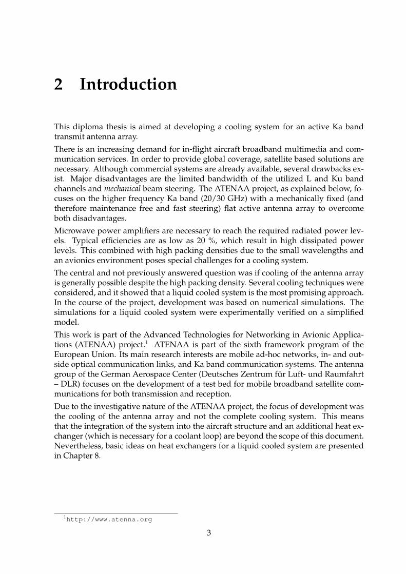
The transmit antenna array operates at about 30 GHz. The radiating elements, patches,are positioned on a flat surface each one half of a free-space wavelength or 5 mm [1] ascan be seen in Fig. 3.1. The elements are arranged in a square. The more patches, thebetter is the antenna performance in terms of directivity. Although different numbersof elements are possible, an array with 50 × 50 elements (and therefore a base plate di-mension of 25× 25 cm2) seems to be the most likely choice at this stage of the ATENAAproject. An array with up to 100 × 100 elements is possible as well.
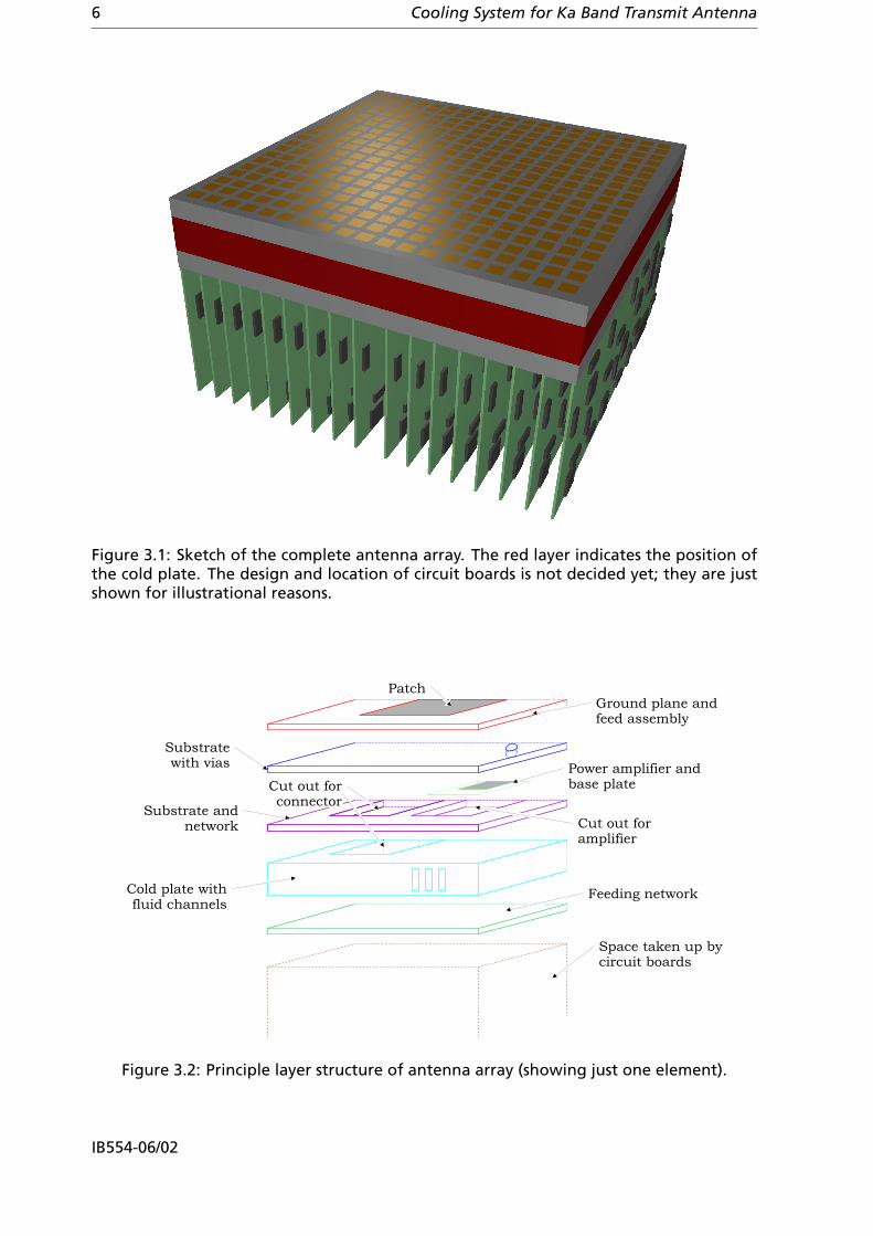
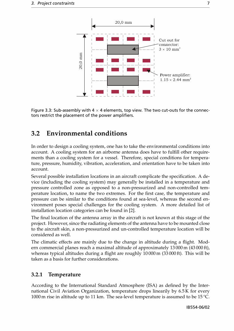
Due to the small wavelength and a resulting high packaging density, integration of allrequired parts including the cooling system is a major problem. Figure 3.2 outlines theprinciple layer structure of the antenna array. The topmost layer (neglecting a possibleradom) is the substrate with the radiating patch. It is connected by vias or by meansof aperture coupling to a layer featuring a network and the power amplifiers. Thepower amplifiers are directly mounted on a yet to be specified cold plate. The poweramplifiers are connected to the feeding network using connectors. Therefore, the coldplate has to incorporate cut outs which will feature the connectors. Although their finaldimensions might still change during the course of the project, they are assumed to be3 mm wide and 10 mm long. Furthermore, the connectors are assumed to be able tobridge a cold-plate thickness of maximal 5 mm. Two connectors will be necessary for asub-assembly of 4 × 4 radiating elements as shown in Fig. 3.3. The cut outs diminishthe available surface area, and therefore the amplifiers have to be placed closer to eachother. Furthermore, the cut outs limit the available locations for fluid channels throughthe cold plate.
No cooling system elements can be placed in the direction in which the antenna radi-ates since the antenna pattern would be significantly influenced. The same is true forthe bottom side since all space is taken up by electronics as indicated in Figs. 3.1 and3.2. Therefore, heat has to be transfered to the sides of the array where it can finallybe dissipated. This and a maximal cold plate thickness of 5 mm are the main factorswhich govern the final cold plate design.
An apparent disadvantage of these constraints is that no heat can be extracted fromseveral spots in the middle of the array. This increases the temperature differenceacross the array which can produce phase errors. This is due to the amplifiers whoseoperating points are affected by temperature. Temperature differences across the arraycan nevertheless be compensated to some degree by calibration of the array.
5
6 Cooling System for Ka Band Transmit Antenna
Figure 3.1: Sketch of the complete antenna array. The red layer indicates the position ofthe cold plate. The design and location of circuit boards is not decided yet; they are justshown for illustrational reasons.
PatchGround plane andfeed assembly
Substratewith vias Power amplifier and
base plate
Substrate andnetwork
Cut out forconnector
Cut out foramplifier
Cold plate withfluid channels
Feeding network
Space taken up bycircuit boards
Figure 3.2: Principle layer structure of antenna array (showing just one element).
IB554-06/02
3. Project constraints 7
Figure 3.3: Sub-assembly with 4 × 4 elements, top view. The two cut-outs for the connec-tors restrict the placement of the power amplifiers.
3.2 Environmental conditions
In order to design a cooling system, one has to take the environmental conditions intoaccount. A cooling system for an airborne antenna does have to fulfill other require-ments than a cooling system for a vessel. Therefore, special conditions for tempera-ture, pressure, humidity, vibration, acceleration, and orientation have to be taken intoaccount.
Several possible installation locations in an aircraft complicate the specification. A de-vice (including the cooling system) may generally be installed in a temperature andpressure controlled zone as opposed to a non-pressurized and non-controlled tem-perature location, to name the two extremes. For the first case, the temperature andpressure can be similar to the conditions found at sea-level, whereas the second en-vironment poses special challenges for the cooling system. A more detailed list ofinstallation location categories can be found in [2].
The final location of the antenna array in the aircraft is not known at this stage of theproject. However, since the radiating elements of the antenna have to be mounted closeto the aircraft skin, a non-pressurized and un-controlled temperature location will beconsidered as well.
The climatic effects are mainly due to the change in altitude during a flight. Mod-ern commercial planes reach a maximal altitude of approximately 13 000 m (43 000 ft),whereas typical altitudes during a flight are roughly 10 000 m (33 000 ft). This will betaken as a basis for further considerations.
3.2.1 Temperature
According to the International Standard Atmosphere (ISA) as defined by the Inter-national Civil Aviation Organization, temperature drops linearily by 6.5 K for every1000 m rise in altitude up to 11 km. The sea-level temperature is assumed to be 15 °C.
IB554-06/02
8 Cooling System for Ka Band Transmit Antenna
0 2.5 5 7.5 10 12.5 15Altitude (in km)
-80
-60
-40
-20
0
20
40
Tem
pera
ture
(in
deg
C)
Standard
Warm climate
Cold climate
(a) Standard (ISA) and other realistic tempera-tures over altitude.
0 2.5 5 7.5 10 12.5 15Altitude (in km)
0
200
400
600
800
1000
Pres
sure
(in
hPa
)
(b) Variation of atmospheric pressure with alti-tude (average sea level pressure is 1013,25 hPa).
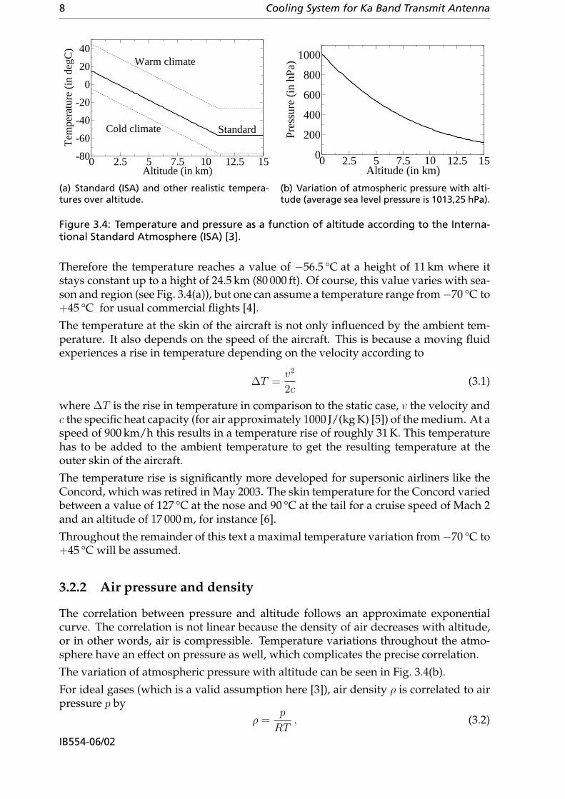
Figure 3.4: Temperature and pressure as a function of altitude according to the Interna-tional Standard Atmosphere (ISA) [3].
Therefore the temperature reaches a value of −56.5 °C at a height of 11 km where itstays constant up to a hight of 24.5 km (80 000 ft). Of course, this value varies with sea-son and region (see Fig. 3.4(a)), but one can assume a temperature range from−70 °C to+45 °C for usual commercial flights [4].
The temperature at the skin of the aircraft is not only influenced by the ambient tem-perature. It also depends on the speed of the aircraft. This is because a moving fluidexperiences a rise in temperature depending on the velocity according to
∆T =v2
2c(3.1)
where ∆T is the rise in temperature in comparison to the static case, v the velocity andc the specific heat capacity (for air approximately 1000 J/(kg K) [5]) of the medium. At aspeed of 900 km/h this results in a temperature rise of roughly 31 K. This temperaturehas to be added to the ambient temperature to get the resulting temperature at theouter skin of the aircraft.
The temperature rise is significantly more developed for supersonic airliners like theConcord, which was retired in May 2003. The skin temperature for the Concord variedbetween a value of 127 °C at the nose and 90 °C at the tail for a cruise speed of Mach 2and an altitude of 17 000 m, for instance [6].
Throughout the remainder of this text a maximal temperature variation from−70 °C to+45 °C will be assumed.
3.2.2 Air pressure and density
The correlation between pressure and altitude follows an approximate exponentialcurve. The correlation is not linear because the density of air decreases with altitude,or in other words, air is compressible. Temperature variations throughout the atmo-sphere have an effect on pressure as well, which complicates the precise correlation.
The variation of atmospheric pressure with altitude can be seen in Fig. 3.4(b).
For ideal gases (which is a valid assumption here [3]), air density ρ is correlated to airpressure p by
ρ =p
RT, (3.2)
IB554-06/02
3. Project constraints 9
where R is the gas constant for a specific gas.1 Therefore, air density and pressure areproportional if the temperature variation over altitude is neglected.
3.2.3 Humidity
The ability of the atmosphere to absorb water depends on the temperature and baro-metric pressure. If either of them is lowered for a saturated atmosphere, the surpluswater condenses out as mist.
As an aircraft is exposed to constantly varying relative humidity, temperature, andbarometric pressure one has to expect water to condense on components and surfacesin open, unpressurized areas. Appropriate steps (like prohibiting the cooling air to bein direct contact with the electronics) have to be taken to avoid corrosion and leakagecurrents.
3.2.4 Mechanical conditions
The cooling system of the antenna has not only to operate properly in harsh climaticconditions but also has to withstand mechanical stresses. Vibrations in an aircraft canbe significantly higher than for a vessel, and comparatively high acceleration and re-tardation takes place. Furthermore, the orientation of the antenna with respect to grav-itation might influence the cooling system performance as well.
These factors have to be considered and can uniquely determine which cooling systemwill be used in the final setup. Orientation and acceleration especially effect heat pipes,which are describe in more detail in Sec. 6.5.
3.3 Amplifier
The antenna array consists of many radiating patches, each of which will be fed by apower amplifier operating at a frequency of about 30 GHz. Choosing an appropriateamplifier depends mostly on the following characteristics: operating frequency range,output power, gain, size, and price. TriQuint’s gallium arsenide monolithic microwaveintegrated circuit (GaAs MMIC) power amplifier TGA4509-EPU [7] seems to be thebest compromise between all characteristics at this stage of the project.
The characteristics which are important for the thermal management are
• chip dimension (length × width × height): 2.44 mm × 1.15 mm × 0.1 mm,
• worst case power dissipation: 3.8 W.
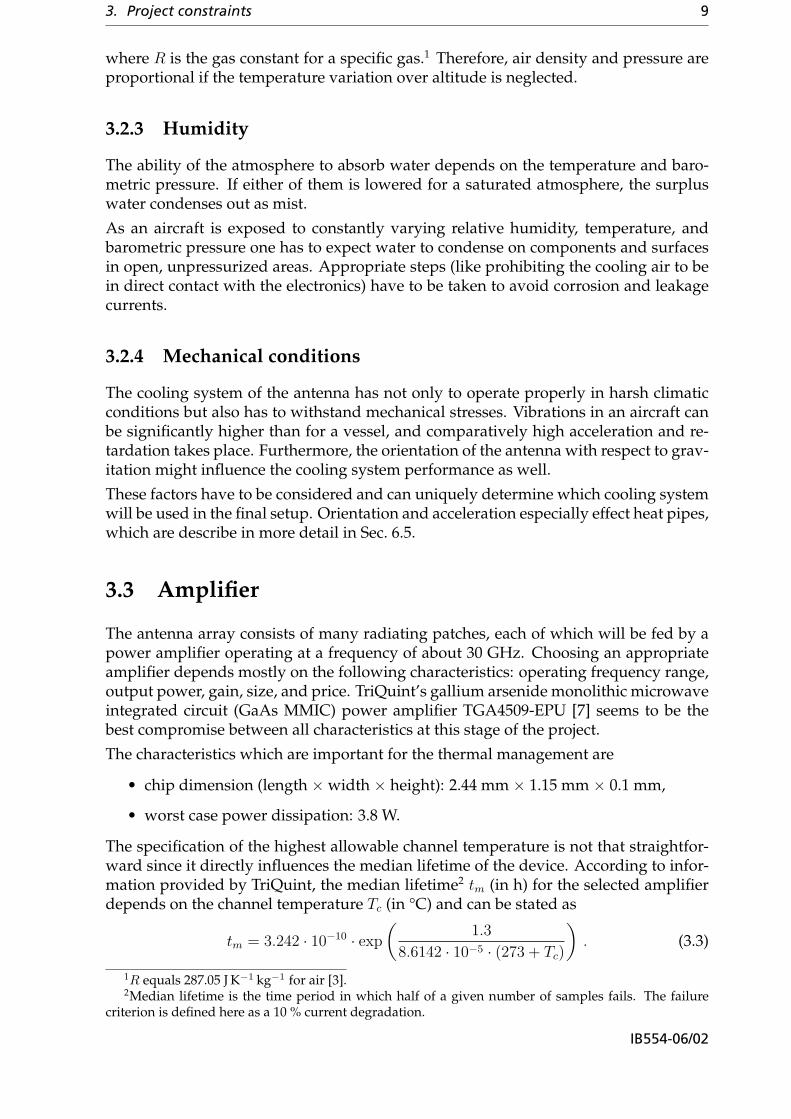
The specification of the highest allowable channel temperature is not that straightfor-ward since it directly influences the median lifetime of the device. According to infor-mation provided by TriQuint, the median lifetime2 tm (in h) for the selected amplifierdepends on the channel temperature Tc (in °C) and can be stated as
tm = 3.242 · 10−10 · exp
(1.3
8.6142 · 10−5 · (273 + Tc)
). (3.3)
1R equals 287.05 J K−1 kg−1 for air [3].2Median lifetime is the time period in which half of a given number of samples fails. The failure
criterion is defined here as a 10 % current degradation.
IB554-06/02
10 Cooling System for Ka Band Transmit Antenna
50 100 150 200 250Channel temperature (in deg C)
1
100
10000
1e+06
1e+08
Med
ian
life
time
(in
year
s)
Figure 3.5: Median lifetime of power amplifier TGA4509-EPU depending on channel tem-perature (see Eq. (3.3)).
The general form of this equation is known as the Arrhenius equation, which describesthe rate at which many chemical processes take place. A graphical representation ofEq. (3.3) can be seen in Fig. 3.5. If a maximal channel temperature of 150 °C is assumed,the median lifetime is 115 years. A channel temperature rise of 5 °C results in a medianlifetime of 76 years.
The conclusion from Eq. (3.3) is that the highest allowable channel temperature is not afixed value, and that lower channel temperatures lead to longer median lifetimes. Al-though a maximal channel temperature of 150 °C is desirable, the amplifier is operatedby TriQuint at channel temperatures up to 275 °C for reliability testings.
The amplifier will be used in an active antenna array. If different amplifiers in the ar-ray work at different operating points, the resulting antenna beam might be negativelyinfluenced. The operating point depends among other things on the operating tem-perature. The temperature coefficient of the proposed amplifier is 0.0135 dB/K at the1 dB compression point for a nominal temperature range of −40 to +85 °C. Hence, atemperature difference of 10 K for two given amplifiers results in 0.135 dB (or 3.2 %)difference in gain. This difference is acceptable since it can be compensated by cali-bration, and a maximal temperature difference between two amplifiers of 10 K will bepart of the specification.
Mounting. TriQuint, the amplifier manufacturer, recommends to solder the ampli-fier to a 0.5 mm thick CuMo (15 %/85 %) base plate to match coefficients of thermalexpansion (also see Sec. 3.4). The die should be soldered using an AuSn (80 %/20 %)eutectic solder preform, which has a melting point of 280 °C3 and provides for goodjoint strengths [8]. A solder preform is a geometrically well defined piece of soldershaped accordingly to the die dimensions. The MMIC is heated until the solder meltsand bonds it to the base plate.
TriQuint’s further recommendation is to attach this sub-assembly by means of epoxyor a lower temperature solder to the module floor or housing. Since many amplifierswill be placed closely next to each other, a heat sink will take the place of the hous-ing. TriQuint states that this attachment method leads to an overall thermal resistance
3The 30 second mounting temperature of the power amplifier is 320 °C.
IB554-06/02

3. Project constraints 11
Material 200 K 250 K 300 K 350 K
Aluminum 20.0 21.9 23.2 24.1 [9]Copper 15.1 16.1 16.8 17.3 [9]GaAs 5.0 5.5 5.8 6.0 [10]Iron 10.0 11.0 11.7 12.1 [9]Kovar 5.0 5.0 [9]Silver 17.7 18.6 19.2 19.6 [9]
AlSiC (60 % v/v SiC) @ 300 to 450 K: 6.5 to 9.0 [11]Brass @ 300 to 400 K: 16.9 to 19.7 [9]CuMo @ 300 to 450 K: 7.0 to 8.0 [12]CuW @ 300 to 450 K: 6.5 to 8.3 [12]
Table 3.1: Coefficient of thermal expansion α at different temperatures in 10-6K-1.
of 22.4 K/W between the channel and the housing. Taking the worst case power dis-sipation of 3.8 W and a median lifetime of 115 years into account, the housing (andtherefore the heat sink) temperature should not exceed 65 °C.
3.4 Heat spreader and heat sink materials
Heat dissipating dice are often not directly mounted to the heat sink but first to a heatspreader. Usually one thinks of a head spreader as of a flat plate of material which hasideally a higher thermal conductivity than the material used for the heat sink. The headspreader ensures a more uniform temperature distribution along the die back. Even ifthe thermal conductivity is not too high, it can become necessary to mount the die notdirectly to the heat sink. This is due to different coefficients of thermal expansion (CTE)for the semiconductor and the heat sink. Mechanical stresses caused by temperaturevariations can lead to device failures. Ideally the CTEs of the semiconductor and theheat spreader (or base plate) should be matched to avoid mechanical stresses aftermounting. Table 3.1 lists the CTEs of some materials.
Investigations have shown that for GaAs dice AuSn soldered to a heat spreader tensilestresses are much more severe than compressive stresses [13]. Therefore, mountinga GaAs component on Kovar (which has a slightly lower CTE than GaAs) results infailures after several thermal cycles. Soldering the GaAs device on CuMo, AlSiC, andCuW (and therefore on materials with a CTE of up to 10.5 · 10−6 K−1) did not lead toany failures. The same investigation confirmed that mounting GaAs devices directlyon copper (which has a conveniently high thermal conductivity) leads to failures.
According to the manufacturer, a direct adhesive attach of the GaAs MMIC as de-scribed in Sec. 3.3 is possible but not recommended. Generally, a thicker adhesivelayer will reduce mechanical stresses on the die since it can better counterbalance thedifferent CTEs. On the other hand, one has to consider that from the thermal pointof view the adhesive layer should be as thin as possible to reduce thermal resistance.Additionally, thermal resistance of the adhesive is not independent of the number ofthermal cycles [14]. Increasing numbers of thermal cycles lead to an increased thermalresistance. While this effect highly depends on the specific adhesive in use, the effectshould be taken into account. It is most pronounced for large differences in CTEs ofthe die and the base plate.
IB554-06/02

12 Cooling System for Ka Band Transmit Antenna
Material 273 K 373 K
Aluminum 238 230 [9]AlSiC (60 % v/v SiC) 200 160 [11]Brass 120 [9]Copper 400 380 [9]Iron 82 69 [9]Silver 418 417 [9]
CuMo @ 300 K: 160 to 170 [12]CuW @ 300 K: 180 to 200 [12]GaAs @ 300 K: 54 [15]Kovar @ 300 K: 11 to 17 [12]
Table 3.2: Thermal conductivity λ in W/(m·K) depending on temperature.
Material Density in g/cm3
Aluminum 2.70 [16]AlSiC (60 % v/v SiC) 3.0 [11]Brass (30 % Zn) 8.55 [17]Copper 8.96 [16]CuMo 10 [12]CuW 15.7 to 17.0 [12]GaAs 5.32 [18]Iron 7.87 [16]Kovar 8.1 [12]Silver 10.45 [16]
Table 3.3: Densities.
Having discussed the coefficient of thermal expansion, another important factor de-termining the appropriate material is the thermal conductivity λ, which should be ashigh as possible. The thermal conductivities of some materials are given in Tab. 3.2.As mentioned before, the die can be mounted to the heat sink in two fashions: withor without a base plate (head spreader). As described in more detail in Sec. 4.1, thecorrelation between plate thickness and thermal resistance is linear. If the thickness ofthe base plate is small (and values down to 0.1 mm are feasible), the overall thermalresistance can still be small despite lower values of thermal conductivity. The influenceof a thin base plate on the overall thermal performance is limited. Since heat sinks arerather large and thick, thermal conductivity becomes a more important factor to reducethe spreading resistance.
Overall weight is important for aerospace applications. Weight can be lessened byreducing system size and by choosing low density materials. The densities of somematerials are listed in Tab. 3.3.
Conclusion. If the amplifier is mounted according to the manufacturer’s recommen-dation (as described in Sec. 3.3, also see [19]), the base plate material does not have tomatch the coefficients of thermal expansion. This allows for discarding special com-pounds like CuW and CuMo. Thermal conductivity, weight, ease of machining, andprice are the remaining major factors.
IB554-06/02

3. Project constraints 13
Copper is the material which has the second highest thermal conductivity (after silver)of all metals. A very good thermal performance can be expected. The only drawbackof copper is its high density. Aluminum, whose density is about 30 % of the density ofcopper, is a good alternative although its thermal conductivity is reduced by 40 % asopposed to copper. Another advantage of aluminum over copper is that it is easier tomachine.
Considering the size of the cold plate, it will make up a major part of the antenna. Bothcopper and aluminum allow mounting of components to the cold plate, which can actas a strong mechanical support.
Copper was chosen to build up a demonstration model, which is described in Sec. 7.1.
IB554-06/02


4 Heat transfer theory
There are three heat transfer mechanisms to be distinguished: heat conduction, con-vection, and radiation. Usually more than one mechanism becomes effective at thesame time, but it is convenient to analyze and describe each of them separately.
4.1 Heat conduction
Thermal conduction works without the transport of a medium by means of atomicand molecular interaction. Heat conduction occurs in solid, liquid, and gaseous mediawhenever a temperature gradient occurs. The correlation between the heat flux densityvector q and the temperature gradient was stated by Fourier as [20]
q = −λ∇T , (4.1)
where λ is the thermal conductivity and T the temperature. The negative sign inEq. (4.1) states that heat always flows from hot to cold regions. The thermal conduc-tivity λ depends on temperature and pressure. Anisotropic media (e. g. wood) exist,but for all materials which are being considered throughout this text λ is a scalar sincethese materials are isotropic.
For most cases Eq. (4.1) cannot be solved directly because the temperature distributionchanges due to heat transfer. Heat conduction can generally be described by Fourier’spartial differential equation
∂T
∂t= a∇2T , (4.2)
where t is the time and a the thermal diffusivity [20]. The thermal diffusivity dependsuniquely on material properties and is given as
a =λ
ρc, (4.3)
where λ is the thermal conductivity, ρ the density, and c the specific heat capacity.
In the special static case the temperature gradients do not depend upon time. Theantenna array will be used in an aircraft, where ambient temperature changes at allmoments can be assumed to be slow as opposed to the reaction time of the system.Then for each moment the system can be said to be in a static (or quasi-static) state,and Eq. (4.2) simplifies to
0 = ∇2T . (4.4)
If the temperature distribution just depends on one variable (which is the case for aplane wall), namely x, Eq. (4.4) can be further simplified to
0 =d2T
dx2. (4.5)
15
16 Cooling System for Ka Band Transmit Antenna
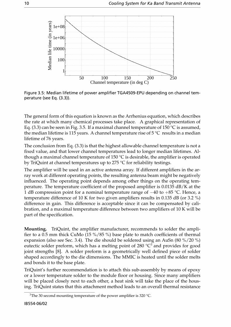
(a) Plane wall with thickness l. (b) Equivalent circuit ac-cording to Eq. (4.7).
Figure 4.1: Steady state thermal conduction.
The last equation can be solved by integration and it results in
T (x) = c1x + c2 . (4.6)
If the temperatures at the wall boundaries are given as T1 = T (x = 0) and T2 = T (x =l) as shown in Fig. 4.1(a), Eq. (4.1) can be rewritten as
Q = λA
l(T1 − T2) =
T1 − T2
Rth
, (4.7)
where Q is the heat flux. This equation is known as the equation of static heat conduc-tion. The thermal resistance Rth for a plane wall is given as
Rth =l
λA. (4.8)
In analogy to steady currents in electrodynamics, statical thermal problems can nowbe depicted and analyzed with the same tools and techniques which are common inelectrical engineering. Ohm’s law in electrodynamics corresponds to Eq. (4.7) in ther-modynamics; the electrical current corresponds to the thermal current Q, the potentialdifference to the temperature difference T1 − T2, and the electrical resistance to thethermal resistance Rth. Figure 4.1(b) shows the equivalent thermal circuit of the afore-mentioned steady case. Using Kirchhoff’s laws, equivalent thermal resistances can befound for more complicated problems consisting of several plates. The configurationcan be depicted in schematic diagrams which are often used in electrical engineering.
The thermal conductivity λ of metals is due to two approximately independent factors:lattice vibrations and movement of electrons. This can be summarized as [21]
λ = λe + λl . (4.9)
Thermal conductivity due to electron movements λe dominates for metals and corre-lates to electrical conductivity by
λe = LcσT , (4.10)
where σ is the electrical conductivity and Lc is the Lorenz constant given as 2.45 ·10−8 V2K−2 [21].
IB554-06/02

4. Heat transfer theory 17
4.2 Convection
As opposed to heat conduction, convective heat transfer is due to a moving fluid, i. e.gas or liquid. Generally, one distinguishes between natural and forced convection. Thefluid moves without any additionally applied force for natural convection, and fluidflow is imposed by by a pump, fan, or other machinery for forced convection. In thefollowing section the special case of heat transfer between a solid and a fluid will bepresented.
The mathematical analysis of convective heat transfer involves the solution of a cou-pled set of partial differential equations to describe the temperature, velocity, and pres-sure fields. The vector velocity field results from the Navier-Stokes equations, whichstates the balance of forces for an infinitesimal element of an uncompressible fluid [22].A general analytical solution has not been found and analytical solutions only exist forspecial cases. Numerical simulations can be used to approximate a solution.
The convective heat transfer between an isothermal surface and a fluid is empiricallydescribed in Newton’s law of cooling
q = h(Tw − T∞) , (4.11)
where Tw is the plate temperature and T∞ the homogeneous temperature of the sur-rounding fluid. The heat transfer coefficient h describes the interface between the sur-face and the fluid. It depends on the heat sink geometry as well as on fluid and flowproperties. The thermal resistance is given as [5]
Rth =1
hA. (4.12)
If the fluid temperature is assumed to vary along the surface A, which is the case forheat exchangers, the temperature difference in Eq. (4.11) has to be replaced by a loga-rithmic temperature difference [23]
∆Tlog =To − Ti
ln Tw−Ti
Tw−To
, (4.13)
where Ti and To are the fluid inlet and outlet temperatures, respectively.
Usually two fluid flows are distinguished: laminar and turbulent. Turbulent flow dif-fers from laminar flow as fluid movement in each point is not along one direction.In the eyes of an observer, turbulent flow is complicated and random. Heat transferdepends on the flow type.
4.2.1 Dynamical similarity and dimensionless numbers.
Fluid flow and convective heat transfer are often described by means of dimensionlessnumbers in order to generalize once found results and correlations. The approach isto assert the similarity of two different flows or heat transfer situations. Two differentflows are called similar if there is a constant ratio between geometrical and physicalproperties for every two congruent points.
Some of these numbers are introduced in the following paragraphs.
IB554-06/02

18 Cooling System for Ka Band Transmit Antenna
Reynolds number. The dimensionless Reynolds number characterizes the flow con-dition. For low Reynolds numbers laminar flow results whereas for numbers abovea critical value turbulent flow exists. For circular pipes, the Reynolds number Re isgiven as
Re =vd
ν(4.14)
where v is the fluid velocity, d the pipe diameter, and ν the fuild’s kinematic viscosity.The Reynolds number can also be interpreted as the ratio
Re =Inertia forcesViscous forces
.
Inertia forces describe the fluid’s natural resistance to acceleration whereas viscousforces are due to internal friction of the fluid.
The kinematic viscosity ν is a function of density ρ and dynamic viscosity η,
ν =η
ρ. (4.15)
The critical Reynolds number for pipes below which laminar flow exists is 2300 [23].For 2300 < Re < 104, the flow is considered to be unstable. Fully turbulent flow isassumed for Reynolds numbers above 104.
Non-circular pipe geometries can be calculated by using the hydraulic diameter dh
instead of the circular diameter in Eq. (4.14). The hydraulic diameter is given as
dh = 4A
U, (4.16)
where A is the cross-sectional area and U the wetted perimeter [24]. It is apparent thatthe hydraulic diameter for pipes with quadratic cross sections equals the side length.
Nusselt number. The dimensionless Nusselt1 number describes the improved heattransfer from a surface to a fluid due to convection in contrast to the heat transferbased solely on conduction. It is also called the dimensionless heat transfer coefficientand is given as
Nu =hL
λ, (4.17)
where h is the heat transfer coefficient, L a characteristic length, and λ the thermalconductivity of the fluid. The characteristic length for a flat wall is the distance fromthe wall edge; the characteristic length of a pipe is the hydraulic pipe diameter.
Prandtl number. The Prandtl number is uniquely based on material properties andequals the ratio of the fluid viscosity and thermal diffusivity
Pr =ν
a. (4.18)
Low numbers indicate that heat transfer is dominated by conduction while convectiveheat transfer is described by high numbers.
The Prandtl number of dry air for temperatures from 0 °C to 100 °C is roughly 0.71;for water at 98,1 kPa it ranges from 13.67 at 0 °C over 5.43 at 30 °C down to 1.75 at100 °C [23].
1Wilhelm Nusselt was a German engineer who graduated 1904 from the Technical University Berlin.Later on he worked as a professor at the universities in Karlsruhe and Munich [25].
IB554-06/02

4. Heat transfer theory 19
4.2.2 Natural convection
Natural (or free) convection is caused by buoyancy of a fluid in the earth’s gravitationalfield. The buoyancy is caused by pressure differences, which are due to temperaturegradients.
Heat transfer by free convection (especially with air as the working fluid) would beoften desirable since no additional appliance has to be installed and maintained. How-ever, heat transfer by means of free convection can usually be just considered for smallamounts of dissipated heat. Since gravitation plays an important role in free convec-tion heat sinks, the orientation of the heat sink becomes important as well.
If a natural convection heat sink is operated in an unpressurized area in an aircraft,pressure and temperature changes due to altitude variations during the flight have tobe taken into account.
Empirical solutions based on dimensionless numbers for heat transfer by natural con-vection have been presented in the literature [20, 23, 26]. As an example, results for ahorizontal flat isothermal plate will be presented in Sec. 6.1.
4.2.3 Forced convection
Fluid flow for forced convection is initiated by some kind of machinery like a pump,fan, or blower to name a few. Natural convection can be neglected in most cases whenanalysing forced convection fluid flow.
Although different schemes for heat transfer by means of forced convection are con-ceivable, the focus will be on heat transfer from a solid wall (like a pipe wall) to a fluid.The most simple case is a flow parallel to a flat wall. The flow will be influenced bythe wall due to the fluid friction, which is described by fluid viscosity. Directly at theboundary, the velocity decreases to zero. The flow velocity approaches the initial ve-locity (which occurred before the plate was entered) a certain distance away from theboundary, see Fig. 4.2(a). This boundary layer thickness is denoted δ. If the wall has adifferent temperature than the fluid, a temperature boundary layer with thickness δT
exists. For liquids (Pr > 1), it yields that δT < δ [23].
If one simplifying assumes that the heat transfer in the temperature boundary layer issolely based on conduction, Eqs. (4.7) and (4.11) lead to
h =λ
δT
. (4.19)
Therefore, in order to assess the heat transfer from a surface, one has to know the fluid’sthermal conductivity and the thermal boundary layer thickness. The Nusselt numberin Eq. (4.15) can now be expressed as
Nu =L
δT
. (4.20)
Boundary layers exist as well in pipe flow, which is more relevant in this context thanflow along a wall. Pipe flow occurs in liquid cold plates, for instance. It will be de-scribed in more detail in the following paragraphs.
Laminar pipe flow. The velocity and temperature profiles for laminar pipe flow areparabolic [23]. They are exemplary shown in Fig. 4.2(b). The Nusselt number (and
IB554-06/02

20 Cooling System for Ka Band Transmit Antenna
v
v = 0
T
Tw
v T
v T
(a) Flow along wall, fluid is a liquid (δT <δ), after [23].
v
v = 0
T
Tw
v T
v T
(b) Laminar flow through pipe, af-ter [23].
v
v = 0
T
Tw
v T
v T
(c) Turbulent flow through pipe, af-ter [27, 24].
Figure 4.2: Velocity and temperature profiles for fully developed flows. The wall temper-ature is higher than the fluid temperature.
therefore the heat transfer coefficient h) can be analytically found. It is given as [28]
Nu =
4.36 for constant heat flux density along the wall3.66 for constant temperature along the wall. (4.21)
It has to be noted that the heat transfer coefficient does not depend on fluid velocityfor laminar flow. Wall roughness has no influence on heat transfer.
Turbulent pipe flow. As opposed to laminar flow, turbulent flow cannot be analyt-ically described. Equations are therefore based on experiments, and stated functionsdiffer in literature.
The velocity and temperature profiles of fully-developed turbulent flow are shown inFig. 4.2(c). It can be seen that both the velocity and the temperature are nearly constantin the center of the pipe. In the region close to the walls, laminar flow exists. Thisexplains the higher temperature difference close to the walls.
For fully-developed turbulent flow in a circular duct, the Nusselt number can be ap-proximated as [23]
Nu ≈ 0.0235 · Re0.8 · Pr 0.48 (4.22)
for 104 < Re < 106 and 0.6 < Pr < 50. Wall roughness (as described by the dragcoefficient) influences heat transfer; the rougher the wall, the better the heat transfer.Equation (4.22) is valid for smooth walls and defines a lower boundary for the Nusseltnumber.
IB554-06/02
4. Heat transfer theory 21
v
v = 0
T
Tw
v T
v T
v
xe
Laminar Transition Turbulent
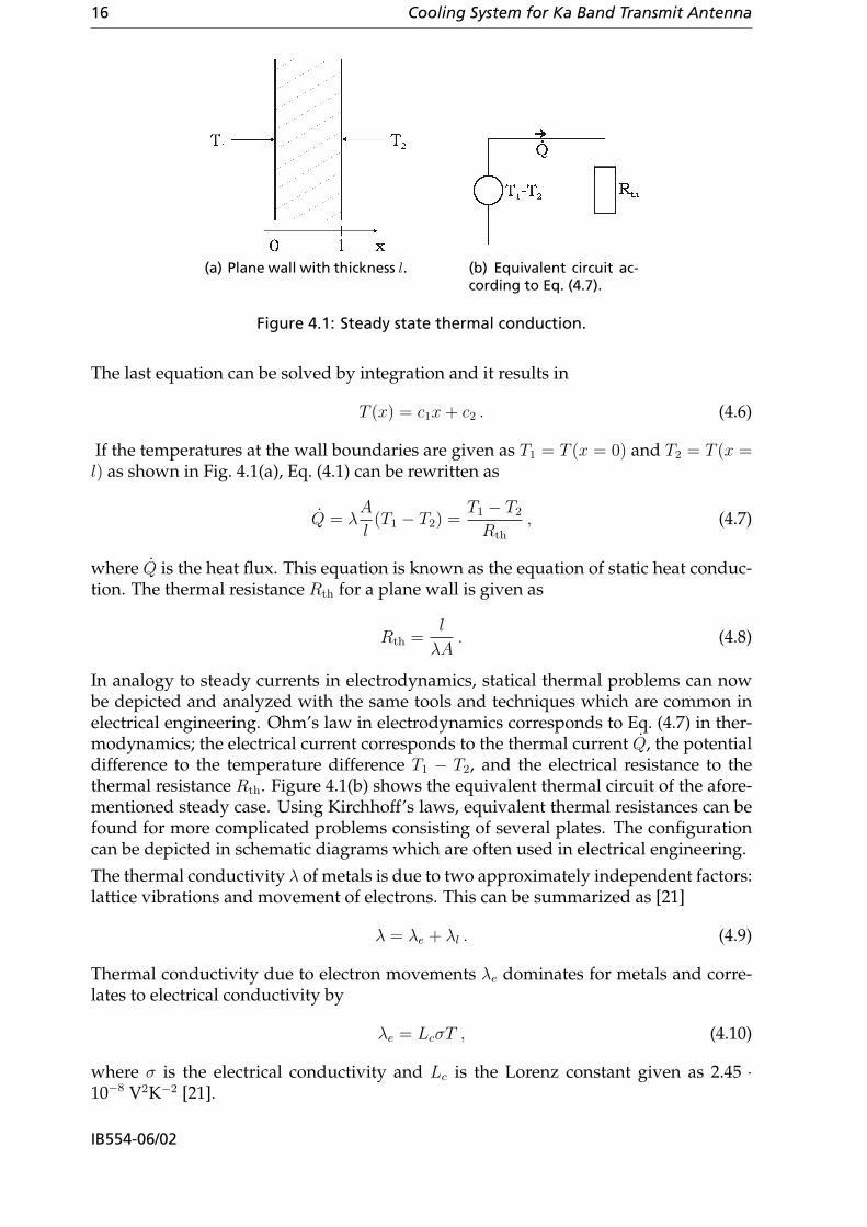
Figure 4.3: Entrance region for turbulent flow, after [23].
Heat transfer is immensely improved for turbulent flow as opposed to the laminarflow case. A simple numerical example for water shows this. Fully turbulent flow isassumed to occur for Reynolds numbers above 104. The Prandlt number for water at50 °C is 3.57 [23]. It follows after Eq. (4.22) that Nu = 84 for turbulent flow, whereas theNusselt number for laminar flow as given in Eq. (4.21) is significantly lower. Therefore,turbulent flow is the preferred flow type for heat exchangers, which comes at a cost ofa higher flow resistance so that more powerful pumps have to be utilized.
Entrance region. If a fluid enters a heated pipe, it takes a certain distance until thevelocity profiles (as shown in Figs. 4.2(b) and 4.2(c)) are fully developed. This regionis called the hydrodynamic entrance region, and its length is denoted as xe. For flowsapproaching both the laminar and turbulent case, the flow near the walls after theentrance is laminar. For turbulent flow, turbulent components first occur after a certainlength as shown in Fig. 4.3. This transitional region is followed by the region of fully-developed turbulent flow.
For laminar flow, the hydrodynamic entrance region xe is given as [28]
xe = 0.056 · Re · d . (4.23)
For non-circular pipes, the pipe diameter d has to be substituted with the hydraulicdiameter according to Eq. (4.16).
The entrance region for turbulent flow is short in comparison to the laminar flow casedue to the better mixing of the fluid. It is given as [28]
10 ≤ xe
d< 60 . (4.24)
Since turbulent flow is desirable for most heat exchanger configurations, one can con-sider to increase the pipe length at the entrance by xe. This would result in an alreadydeveloped turbulent velocity profile when the flow reaches the heated region. Thiswould mean that a high heat transfer is ensured for the whole heated pipe surface.
Fin efficiency. Fins are often used to increase the convective heat transfer by increas-ing the contact area between the solid and the fluid. The heat transfer does not increaseproportionally with the contact area since the temperature from the base to the tip of
IB554-06/02
22 Cooling System for Ka Band Transmit Antenna
the fin decreases due to the limited thermal conductivity of the material. The fin effi-ciency factor describes the heat flow of an actual fin to the theoretical heat flow of anisothermal fin.
4.3 Thermal radiation
As opposed to heat conductance and convection, no additional medium is necessaryfor heat transfer by means of electromagnetic radiation. Although every object witha temperature above absolute zero emits thermal radiation, the spectrum and powerdepends on the object’s properties and its absolute temperature. Even slight changes inthe surface properties of an object can highly influence the thermal radiation. In orderto simplify the analysis, one consideres a special kind of radiating object, a blackbody.
A blackbody is a hypothetical object which is able to absorb all incident radiation.Since Kirchoff’s law of radiation states that the emissivity of an object is equal to its ab-sorbance at the same temperature, a blackbody also emits maximal thermal radiation.The power P emitted by a blackbody is given by the Stefan-Boltzmann law
P = σAT 4 , (4.25)
where σ is the Stefan-Boltzmann constant given as 5.67 · 10−8 Js−1m−2K−4, A the totalradiating area, and T the absolute temperature.
Example. The maximal possible radiated energy from an antenna element can be as-sessed even if no specific surface shall be assumed at this point. This is possible if oneassumes the antenna element to be a blackbody.
The antenna element under consideration consists of a quadratic ground plate with anedge length of 5 mm. Mounted on one side of the ground plate is the heat dissipatingamplifier. Since many antenna elements will be mounted directly next to each other, noradiation can occur to the sides of most of the antenna elements. Therefore, radiationto the sides will be neglected here. Two radiating surfaces per element are remaining,the top and bottom surfaces.
If one assumes that the amplifier has a temperature of 100 °C and using Eq. (4.25), each(blackbody) surface radiates a power of 27.5 mW. This totals to 1.45 % of the formerlyassumed 3.8 W maximal power dissipated by the amplifier.
Considering that a real body with a less than ideal surface will radiate even less energy,it becomes apparent that the heat dissipated by the amplifier cannot be transfered bymeans of radiation.
Due to the small portion of power which is being radiated as opposed to the powerbeing dissipated by the amplifier, thermal radiation will be neglected in the remainderof this text.
IB554-06/02

5 Software
Numerical simulations are one possibility to approach problems in thermal and fluiddynamics. Several advantages and shortcomings arise.
The governing equations of thermodynamics, as described in Sec. 4, cannot generallybe solved. While empirical equations exist to describe certain simple geometries, andanalytical solutions were found for special cases [22], numerical simulations offer ageneralized approach to approximate solutions for any given geometry. Numericalsimulations are advantageous when numerical models can be build with less practicaland financial strains than real-world prototypes. This is especially true for environ-ments in which prototypes cannot easily be examined, namely low or high temper-atures and altitudes. Furthermore, numerical models can usually be modified withrelative ease and allow for a quick optimization. Early rough numerical models canhighlight future problematic aspects of a design and can speed up the optimizationprocess.
On the other hand, numerical simulations are always based on certain assumptionsconcerning boundary conditions and material properties. Wrong or imprecise assump-tions can easily lead to erroneous solutions, and great care has to be taken at this stageof the simulation. Although measurement uncertainties do not exist in numerical sim-ulations, the overall solution is just an approximation of the real world situation. Thisis due to the fact that the solution domain is somehow discretized, and the solutiondepends on the discretization. While finer grids can introduce new problems, theyusually lead to more precise solutions. The drawback is an increase in computer andtime resources. Therefore, a compromise has to be found.
In the following two sections, the commercial software packages Flotherm1 and Ther-mal Desktop2 (utilizing Sinda/Fluint) will be presented. It will be highlighted whyFlotherm was chosen to conduct numerical simulations for this project.
5.1 Thermal Desktop
Thermal Desktop is a CAD based thermal modeling software [29]. The software de-scribes a given geometry as a network of lumps and solves it using the thermal andfluid network solver Sinda/Fluint. For the one-dimensional steady state case, the net-work representation would look similar to Fig. 4.1(b) on p. 16. In order to simulatetransient cases, further elements, which would be called capacitors in the electrody-namics equivalent, are added.
Convective heat transfer and fluid flows are treated empirically. The software makes
1FLOTHERM® is a registered trademark of Flomerics Ltd.2Thermal Desktop® is a registered trademark of Cullimore & Ring Technologies, Inc.
23
24 Cooling System for Ka Band Transmit Antenna
use of the dimensionless numbers as described in Sec. 4.2.1. This approach leads to fastresults as opposed to computational fluid dynamics (CFD) calculations [30]. However,the empirical approach is its major drawback since assumptions have to be made to beable to apply the empirical formulas. For instance, convection is limited to cases withvertically or horizontally aligned walls, and flows are assumed to be fully developed.
A thermal network representation is well suited to one-dimensional problems. A pip-ing loop is one example, or geometries with thin walls. Thin means in this case that thewall can be assumed isothermal. Whenever thermal distributions inside a wall becomeimportant, as it is the case for heat spreaders, a full discretization of the solution do-main is better suited. The same is true for arbitrary flows, which cannot be describedempirically.
5.2 Flotherm
Flotherm [31] is based on computational fluid dynamics to compute heat transfer forheat conduction, forced, and free convection, and radiation. Its main advantage is thepossibility to predict fluid flows, both laminar and turbulent. As opposed to ThermalDesktop, splitting flows as well as flows around obstacles like fins can be modeled.This comes at a cost of an increased demand for time and computer resources.
Instead of representing a geometry as a thermal network, the whole solution domain isbeing discretized on a Cartesian mesh. The governing differential equations, which arepartly described in Sec. 4, are being solved directly. No additional assumptions haveto be made in order to get an approximate solution.
Several sources of error in modeling a given geometry exist. Since a Cartesian grid isused, only rectangular geometries can be modeled precisely. Oblique, bent, and curvedsurfaces have to be approximated by many cubes or prisms, for instance. Although ma-terial properties can be accurately specified, they are often not exactly known. Initialassumptions can often be rough, which is another reason for an imprecise solution.
Defining an appropriate grid is one of the main challenges in using the software.Whereas a rough grid leads to fast computations, a fine grid is necessary to modelareas with high temperature, pressure, and velocity gradients. Generally, a finer gridleads to better accuracy. The grid does not have to be uniform, and several tools existto simplify grid definition. For instance, the grid can be refined just locally in areaswhich are assumed to contain high gradients or which are of special importance. Theoverall accuracy in comparison to a non-localized grid is being preserved [32]. Cellswith large aspect ratios and large changes in cell dimensions of adjacent cells shouldbe avoided. Smoothing algorithms help to achieve this.
It became apparent that Flotherm should be chosen for this project. This allows arbi-trary fluid flows to be calculated, which occurred at the fluid inlets, for instance.
IB554-06/02

6 Cooling techniques
Several cooling techniques are available. Some cooling techniques, ordered roughly byincreasing cooling effectiveness and complexity, are:
1. Natural convection air cooling
2. Forced convection air cooling
3. Cooling utilizing heat pipes
4. Liquid cold plates
5. Micro-channel liquid cold plates
Each technique offers advantages and disadvantages, which define the final choice.Often more than one choice is feasible, but for most commercial cases the least complexsolution is used since it usually involves the lowest costs. Deviation from this ruleoccurs when costs play a minor role. Weight and reliability, for instance, are importantfor space- and airborne applications.
6.1 Natural convection air cooling
The following two examples will demonstrate that a heat sink based on natural convec-tion does not provide the necessary cooling effectiveness for the antenna array underconsideration.
Empirical formulas will be used, which limit the analysis to some specific geometries.Here, a horizontal flat isothermal plate will be taken as the heat source. The coefficientwhich has to be determined is the heat transfer coefficient h. Once it has been obtained,the convective heat flux density q can be determined by Eq. (4.11). The heat transfercoefficient can be determined by finding the dimensionless Nusselt number accordingto Eq. (4.17),
Nu =hL
λ, (6.1)
where L is the heated plate area divided by the plate circumference and λ the thermalconductivity of the fluid. For a horizontal, flat plate the Nusselt number is also givenas [20]
Nu =
0.766[Raf(Pr)]1/5 for Raf(Pr) < 7 · 104 (laminar flow)0.15[Raf(Pr)]1/3 for Raf(Pr) > 7 · 104 (turbulent flow) (6.2)
withf(Pr) = [1 + (0.322/Pr)11/20]−20/11 , (6.3)
25
26 Cooling System for Ka Band Transmit Antenna
where Ra and Pr are the dimensionless Rayleigh and Prandtl numbers, respectively.
For the first example, an array of 100 × 100 array elements is assumed. Each squareelement has a side length of 5 mm and dissipates 3.8 W. This results in an antennaarray size of 0.25 m2 and the worst case dissipated power totals to 38 kW. The ambientair is assumed to be at T∞ = 20 °C. If the maximal plate temperature is taken as Tw =70 °C, allowing for a temperature difference of 50 °C, the flow is turbulent and the heattransfer coefficient is h = 4.75 Wm−2K−1. According to Eq. (4.11) the total heat flux isonly 60 W, which is about 0.16 % of the total dissipated power in the antenna. Thisresult underlines that cooling by means of natural convection in air is not sufficient,and it does not even add significantly to the overall required heat flux.
In the second numerical example an array size of four by four elements (4 cm2) will beassumed. This conforms to a configuration which might be build as a demonstrationmodel later on in the ATENAA project. The cooling would be improved by simplyincreasing the size of the horizontal base plate, which will be assumed to be isothermalhere (neglecting the finite thermal conductivity of the plate). In order to transfer 42 ·3.8 W of dissipated power, the square plate would have to have a size of 0.256 m2 or aside length of 50.6 cm.
The results of the second example were verified by numerical simulations utilizingFlotherm. A 1 cm thick copper plate was used as the heat spreader, and the assumptionof a nearly isothermal surface was confirmed.
Conclusion. Simple numerical examples showed that cooling based on natural con-vection is not feasible for the antenna array. Choosing a cooling technique other thannatural convection helps to avoid the following problems as well: The heat wouldhave had to be transferred to the sides of the array first since a fin heat sink cannotbe directly implemented where power is dissipated due to assembly constraints as de-scribed in Sec. 3.1. Furthermore, the performance of a possible fin heat sink dependson air density as well as on orientation with respect to the gravitational field. The sys-tem would have had to be designed for the worst case, which would further increaseoverall weight and size.
6.2 Forced air cooling
Air cooling by means of forced convection is realized by air moving devices like fansand blowers. Forced air cooling is a very common choice for many applications sincea cooling system is often low-cost and can comparably easily be build. In an aircraft,basically two environments for forced air cooling are conceivable: the pressurized andcontrolled temperature zone and the non-pressurized and non-controlled temperaturezone. Altitude significantly affects the second environment. The first scenario, a tem-perature and pressure controlled location for the heat sink, simplifies overall designsince different ambient conditions do not have to be taken into account. Since the finallocation of the heat sink in the aircraft has not been decided yet at this stage of theproject, the more general second scenario will be characterized in the following.
The cooling air from outside the aircraft is often conditioned before it is passed fur-ther on to the cooling system. This step is necessary to filter out humidity, dust, andgrease particles. Although this greatly reduces the amount of humidity, humiditymight nevertheless pass on and accumulate on electronic equipment. The humidity
IB554-06/02
6. Cooling techniques 27
can lead to failures, and therefore direct contact of cooling air with electronics shouldbe avoided [26]. This greatly influences the basic design of the cooling system.
One way of collecting fresh air can be by means of an inlet in the outer skin of theaircraft. This ram air can actually be a heat source rather than a coolant. Referringto Sec. 3.2.1, the ambient temperature on a warm day can be 45 °C. The temperatureincrease for a typical cruise speed (900 km/h) is approximately 31 K, according toEq. (3.1). Adding these two numbers up (and neglecting that the cruise speed does notoccur at ground-level) leads to an inlet temperature of 76 °C, which is already abovethe maximal heat sink temperature of 65 °C for the amplifier under consideration (seeSec. 3.3). Therefore, the air pre-conditioning has to include cooling. Different sec-tions of the airplane (passenger cabin, electronics) require different temperatures andpressures. The system regulating the on-board climate is often referred to as the en-vironmental control system (ECS). The air source is often bleed air from the aircraft’sengine compressor stage at a temperature of 300 °C. Air temperatures below 0 °C arenevertheless available [33]. A simple cooling system based on evaporating a controlledamount of water shortly after the ram air intake is presented in [34], which can be usedfor pods being not connected to the ECS, for instance.
The interesting figure in determining the performance of an air cooling system is thetemperature difference between the air inlet and the heat sink hot spot. The tempera-ture rise is due to two factors:
• ∆TA describes the temperature rise of the cooling air as it passes through the heatsink.
• ∆TB is due to the thermal resistance described by the heat transfer coefficientbetween the surface and the moving fluid.
Therefore, the hot spot surface temperature Ts is given as [26]
Ts = Tin + ∆TA + ∆TB , (6.4)
where Tin is the air inlet temperature.
Summand ∆TA. First, the temperature rise ∆TA will be discussed; a good introduc-tion to fan heat sinks is given in [26, 35]. The first step in determining a fan for aforced air cooling is to assess the required volumetric fluid flow rate. It depends onthe specific heat of the fluid. Specific heat c, which is also called specific heat capacity,is the amount of heat required to change one kilogram of a substance by one kelvin.This quantity becomes important if one wants to assess the amount of fluid requiredto ensure a defined maximal temperature difference between the fluid inlet and outlet,here denoted as ∆TA. The following equation results from taking the derivative withrespect to time of the defining equation for specific heat
Q = cm∆TA , (6.5)
where Q is the heat flux, c the specific heat capacity, m the mass flow rate, and ∆TA
the temperature difference between the outlet and inlet. The mass flow rate can beexpressed as
m = ρG , (6.6)
IB554-06/02

28 Cooling System for Ka Band Transmit Antenna
Figure 6.1: Typical fan performance curve. The intersection between the system resistancecurve (dashed) and the fan performance curve defines the operating point.
where G is the volumetric flow rate. Therefore, the mass flow rate is directly propor-tional to density. Now the required volumetric flow rate for a given heat flux andmaximal temperature difference is given as
G =Q
cρ∆T. (6.7)
The volumetric flow rate is not the only characteristic property of fans. A fan canonly provide a certain pressure drop between the inlet and outlet side of the fan. Afan’s performance can be depicted in a fan performance curve, which correlates thevolumetric flow rate and the pressure drop. A typical fan performance curve can beseen in Fig. 6.1. It states that a fan can deliver a high volume flow rate if the airflow isnot obstructed. The airflow can shut off for high flow resistances.
The flow resistance is determined by the system, since the air will have to flow aroundand through components including heat sinks and filters. The system resistance is ameasure of required pressure drop for a given volumetric flow rate. The pressure dropas a function of volumetric flow rate can be expressed as [36]
∆p = klG for laminar flow,∆p = ktρG2 for turbulent flow, (6.8)
where kl and kt are system specific constants for the laminar and turbulent case, re-spectively. The operating point of the fan is determined by the intersection of the fanperformance and system resistance curve (as shown in Fig. 6.1). Once the resistancecurve is known, an appropriate fan can be chosen.
The resistance curve can be derived by
• using empirical formulas (for rather simple geometries),
• measurement of the real system, or
• simulation of the given geometry based on computational fluid dynamics.
The last approach will be used in Sec. 6.2.2.
IB554-06/02
6. Cooling techniques 29
Air filters are often necessary to clear the cooling air from dust particles and other im-purities. A filter can significantly increase the system resistance. In order to minimizethe pressure drop across the filter, the filter surface area should be as large as possible.
Summand ∆TB. The second characteristic number in Eq. (6.4), ∆TB, is governedby Eq. (4.11). The heat transfer coefficient can be determined by empirical formulasfor specific geometries involving dimensionless numbers as defined in Sec. 4.2.1. As-sumptions about flow conditions (e. g. fully developed flow) and a limited amount ofavailable formulas in the literature for different geometries restrict this approach. Forarbitrary geometries and different flow conditions, numerical simulations are used todetermine ∆TB.
6.2.1 Influence of altitude
The influence of altitude on air cooling has been presented in [26, 36, 37].
Influcence on ∆TA. Since the mass of air and not the volume governs the cooling (seeEq. (6.5)), the air density decrease with altitude (as described in Sec. 3.2.2) reduces thecooling effectiveness. In other words, the temperature difference between fluid inletand fluid outlet increases according to
∆Ta =ρ0
ρa
∆T0 , (6.9)
where index 0 indicates the nominal condition at sea level and a the altitude condition.Therefore, the temperature rise is inversely proportional to the air density.
In order to describe the fan performance depending on altitude, so-called fan laws canbe used. They assume constant fan efficiency1 at all operating points and altitudes andcan be stated as [36]
Ga = G0 ·ωa
ω0
(6.10)
∆pa = ∆p0 ·(
ωa
ω0
)2
· ρa
ρo
(6.11)
Pa = P0 ·(
ωa
ω0
)3
· ρa
ρo
(6.12)
where:G volumetric flow rate (m3/s);∆p pressure drop (N/m2);P fan power (W);ω revolutions per minute;ρ density of air (kg/m3);♦a index for condition at specific altitude;♦0 index for nominal condition.
It can be seen that the volumetric flow rate G is independent of air density, whereasthe pressure drop and fan input power are directly proportional to density.
1Fan efficiency is defined as the ratio between useful output power (moving air) and fan input power.
IB554-06/02
30 Cooling System for Ka Band Transmit Antenna
(a) Constant speed fan for turbulent flow.
(b) Altitude compensating fan and turbulentflow.
(c) Altitude compensating fan and laminar flow.The system resistance curve is independent of al-titude for laminar flow.
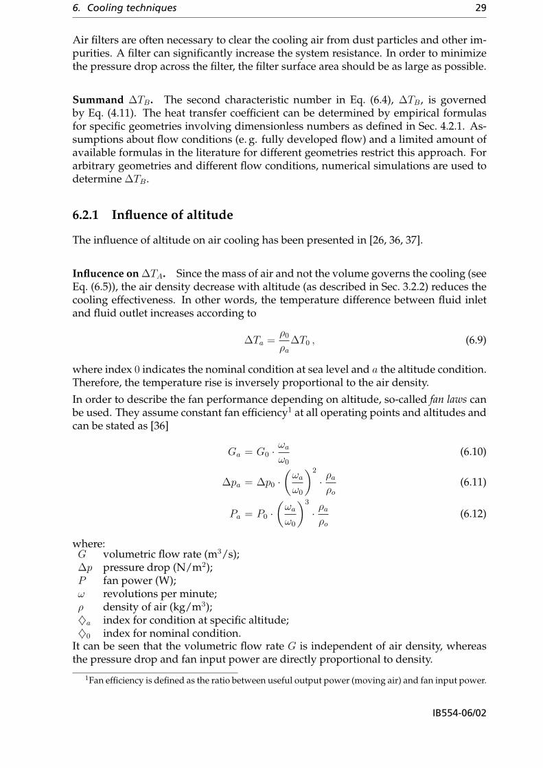
Figure 6.2: Dependence of operating point for the two different fan types. For this ex-ample, the altitude compensating fan is assumed to run at a 30 % increased speed at analtitude of 10 km. System resistance curves are depicted in dashed lines.
There are two different kinds of fans: constant speed fans (also called conventional fans)and altitude compensating fans (also called slip fans). Conventional fans always run atthe same speed, which results in constant volumetric flow rates according to Eq. (6.10).Slip fans partly compensate the decreased density and therefore reduced cooling effec-tiveness at higher altitudes by increasing their speed due to the decreased load on thefan.
While dimensioning the cooling system with a conventional fan for the worst case athigh altitudes is possible, the cooling system would have excess performance at sealevels. This shows in unnecessarily high power consumptions. Depending on the fan,the fan motor’s waste heat is often dissipated by the same fluid flow. Hence, higherpower consumptions lead to higher fluid inlet temperatures. Further disadvantages ofa conventional fan at lower altitude are increased noise and, more important, mechan-ical stresses and wear, which lead to a shorter lifetime. An altitude compensating fan,on the other hand, provides a higher volume flow rate just for lower densities.
Figure 6.2 shows the dependance of the operating point on altitude. As an examplescenario for a conventional fan (Fig. 6.2(a)), the density ratio ρa/ρ0 is about 0.34 foran altitude of 10 km according to the International Standard Atmosphere [3]. This isexactly the ratio by which the pressure difference ∆p and the system resistance for tur-bulent flow will be decreased, according to Eq. (6.11) and (6.8), respectively. Therefore,volumetric flow rate does not depend on altitude for turbulent flow. It has to be noted
IB554-06/02

6. Cooling techniques 31
that the mass flow rate, which is the relevant factor for the cooling effectiveness, isdecreased to the same 34 % according to Eq. (6.6).
An altitude compensating fan behaves differently. The fan speed increases with alti-tude, which is assumed to be 30 % at an altitude of 10 km for this example. The vol-umetric flow rate increases by the same amount, according to Eq. (6.10). The pressuredrop is both affected by speed and density. It decreases by 43 % according to Eq. (6.11).This defines the fan performance curves at 10 km in Fig. 6.2(b) and 6.2(c).
The system resistance curve depends on density and therefore altitude just for turbu-lent flow. The resulting operating points are highlighted in Fig. 6.2(b). The volumetricflow rate increased with altitude, which is an improvement in comparison to the con-stant speed fan.
For laminar flow, the linear system resistance curve does not depend on density asshown in Fig. 6.2(c). Despite the altitude compensating fan, the volumetric flow de-creases for higher altitudes (as opposed to the constant flow rate for a conventionalfan and turbulent flow). This is the reason why a turbulent flow heat sink should beconsidered for unpressurized locations in aircrafts.
Closed-loop controls. An altitude compensating fan runs at different speeds for dif-ferent altitudes, but it does not necessarily completely compensate for the lower den-sity at higher altitudes, depending on system design and fan specifications. An alterna-tive is a conventional fan whose speed is controlled by a closed loop system. Althoughthe overall system still has to be designed for the worst case, the fan does not have tooperate at its maximum for many scenarios.
The feedback circuit is based on one or several sensor outputs, which typically mea-sures the temperature at critical spots in the design. This information can also be usedin order to monitor system performance and to set off an alarm in case of a failure. Asimpler fan-speed sensor could not detect failures in the flow pass, e. g. blocked filters.
The disadvantage of this approach are the increased complexity as another electric cir-cuit is needed. As for any closed loop system, it has to be ensured that the system doesnot oscillate. This should not pose a major challenge due to the rather slow responsesof thermal systems.
Influence of altitude on heat transfer coefficient and therefore ∆TB. The heat trans-fer coefficient h is directly proportional to the Nusselt number, see Eq. (4.17). The Nus-selt number for fully-developed turbulent flow in circular pipes is given in Eq. (4.22).Taking Eq. (4.14) and (4.15) into account and combining constants to C, the heat trans-fer coefficient as a function of density (and therefore altitude) and volumetric flow rateis
h = Cρ0.8G0.8 . (6.13)
It follows that∆TB ∼
1
ρ0.8G0.8. (6.14)
For constant speed fans, the volumetric flow rate does not depend on altitude.
Hot spot surface temperature TS depending on altitude. Cooling effectiveness de-creases with increasing altitude due to a lower air density at higher elevations. Thiseffect is somewhat compensated by a reduced ambient temperature at higher altitudes.
IB554-06/02
32 Cooling System for Ka Band Transmit Antenna
-75
-50
-25
0
25
50
75
100
125
150
175
200
0 2.5 5 7.5 10 12.5 15
Altitude in km
Tem
pera
ture
in °
C
Air inlet temperature
Highest cabinet temperature
Heat sink temperature (turbulent flow)
Critical heat sink temperature (65 °C)
T in,0
∆ T B ,0
∆ T A ,0
(a) Tin,0 = 15 °C, ∆TA,0 = 10 K, ∆TB,0 = 40 K. Heat sink temperature is already exceedingrequirements at about an altitude of 8 km.
-50
-25
0
25
50
75
100
0 2.5 5 7.5 10 12.5 15
Altitude in km
Tem
pera
ture
in °
C
Air inlet temperature
Highest cabinet temperature
Heat sink temperature (turbulent flow)
Critical heat sink temperature (65 °C)
T in,0
∆ T B ,0
∆ T A ,0
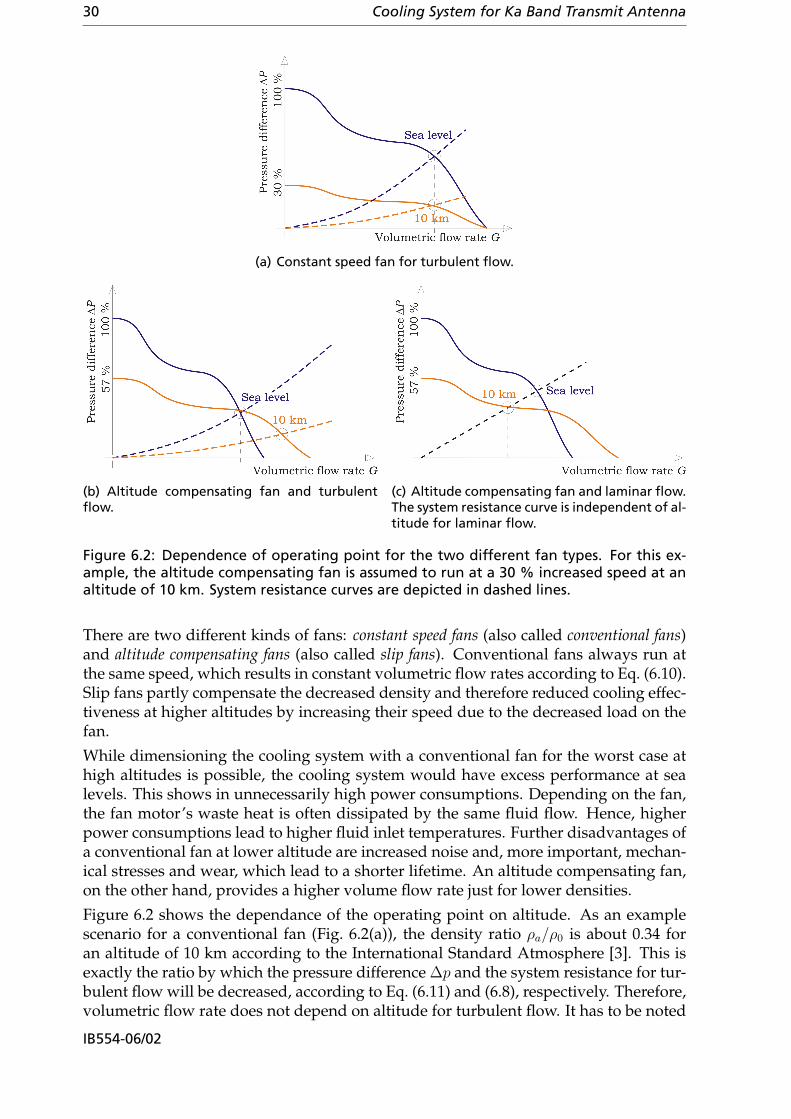
(b) Tin,0 = 40 °C, ∆TA,0 = 5 K, ∆TB,0 = 20 K. Heat sink temperature does not exceedtemperature requirements for altitudes below 14 km.
Figure 6.3: Exemplary dependence of heat sink temperature from altitude for the turbu-lent flow case utilizing a constant speed fan. Two different sets of inlet temperatures Tin
and temperature differences ∆TA,0 and ∆TB,0 at sea-level are assumed.
IB554-06/02

6. Cooling techniques 33
In order to find out if the maximal heat sink temperature of 65 °C (see Sec. 3.3) is ex-ceeded for higher altitudes, the temperature differences ∆TA,0 and ∆TB,0 at sea-levelhave to be known.
Figure 6.3 shows an exemplary correlation for an non-pressurized area. Since ∆TA de-pends on the volumetric flow rate and, simply spoken, therefore on the size of the fan,the figure is chosen to be small. Generally, a larger fan is always an option. ∆TB, on theother hand, depends on the heat sink geometry, which is constricted by assembly con-straints (no direct contact of air with electronics, maximum thickness of 5 mm). Hence,the number was chosen to be large as opposed to ∆TA. As discussed before, the inletair cannot be directly taken from the outside. The preconditioned air is assumed tohave a temperature of 15 °C and 40 °C at sea-levels for Fig. 6.3(a) and 6.3(b), respec-tively. It is assumed that the preconditioning system maintains a fixed temperaturedifference between the outside air inlet and the air which is supplied to the fan inlet.
Figure 6.3(a) shows that the heat sink temperature exceeds the requirements for analtitude above 8 km. The decreasing outside temperature does not compensate thedecreasing air density as is the case for the second example depicted in Fig. 6.3(b).It can be concluded that the influence of altitude can be both positive and negative,depending on the specific system design.
6.2.2 Possible designs and simulations
Heat sinks are usually build out of a material with high thermal conductivity like cop-per or aluminum. They are based on the principle that an increased contact surface forthe fluid increases cooling effectiveness. This is not true by itself as flow resistance andfin efficiency influence the overall performance as well.
Commercially built fin heat sinks belong most often to one of the following categories:
• Extruded heat sinks are made out of a single piece of metal. They are usually low-priced, made out of aluminum, and the most common choice for a variety ofapplications.
• The fins of a folded fin heat sink are made out of a single sheet of material in awavelike manner bonded (solder, braze, or epoxy) to one or two solid plateswhich act as a heat spreader and/or direct the fluid flow. The main advantageare thin fins and the possibility to combine two materials for fins and baseplates.Thin fins are beneficial for thin heat sinks since they allow for a better air flowand reduced weight. For thicker heat sinks, the reduced fin efficiency of thin finsbecomes a disadvantage.
• Bonded heat sink are very similar to folded heat sinks. The difference is that the finsare made out of several plates which are separately bonded to the base plate. Thecritical point of the design is the quality of the joint since it can greatly increasethe thermal resistance.
• Die cast heat sinks, which are mostly made out of aluminum (although copper isanother possible material), can be mass-produced in more complex shapes than itis possible for the other methods mentioned before. The fins cannot be producedas thin as for folded fin heat sinks, for example.
• To overcome the disadvantage of die cast heat sinks, cold forged heat sinks weredeveloped. Thin and high fins can be fabricated.
IB554-06/02

34 Cooling System for Ka Band Transmit Antenna
Figure 6.4: Design 1. The three fluid channels are 1 mm wide and 3 mm high. The coppercold plate is 20 mm long.
• Milled heat sinks are usually expensive, but special geometries made out of a va-riety of materials can be realized.
The fins can be shaped and arranged in many different ways. Often used forms in-clude plate fins and pin fins with square or circular cross-sections arranged in-line orstaggered. The surface is often treated. A black surface increases thermal radiation,which can especially improve cooling efficiency for natural convection heat sinks. Forforced convection heat sinks, this improvement is secondary.
Design 1: Based on liquid cold plate
The first design was numerically simulated in order to verify the basic principles inforced air convection and to get an insight about the accuracy of Flotherm. The utilizedgeometry is the same as the one described in more detail in Sec. 6.3.2 for liquid cooling.The practical thought behind this approach was that the liquid cold plate could beutilized in a forced air cooling system for a smaller demonstration model (like 4 × 4elements instead of 50 × 50 elements) and thereby abandoning the need to install amore complex liquid cooling system.
The ambient air was set to a temperature of 20 °C at sea-level. Many antenna elementswill be placed next to each other in the final design. Due to the repetitive pattern ofthe overall antenna array, only a small stripe (2 elements wide) is necessary for thenumerical model to assess the overall performance while neglecting side effects andassigning symmetry boundaries at the appropriate walls of the computational domain(see Fig. 6.4). Flow restricting walls had to be added to the numerical model in orderto force the air flow through the channels.
Allowing for a maximum temperature difference between inlet and outlet of 10 K, thevolumetric flow rate of the fan was set to 2.83·10−3 m3/s (6 cfm).
In a first run, the volumetric flow rate was set to be constant, neglecting the fan curveand assuming that the fan could provide any amount of pressure difference. The result-ing outflow temperature agreed within 1 K with the expected temperature difference;the heat sink hot spot temperature was 34 °C. Although these results sound promising,
IB554-06/02

6. Cooling techniques 35
the pressure difference required to force the flow through the channels has to be con-sidered as it is substantial. The pressure drop was 60 kPa (0.6 bar), resulting in a flowspeed of 275 m/s inside the channels. This value is beyond any practical application.As a comparison, an exemplary commercial fan with a size of 120 × 112 × 30 mm3 isable to provide a maximum pressure difference of 470 Pa [38].
The fan curve of the previously mentioned commercial fan was taken into account ina second run, which lead to realistic pressure drops across the air inlets and outlets ofthe cold plate. Now the fluid velocity inside the channels is 26 m/s and the outflowtemperature rises to 100 °C. The heat sink hot spot temperature is 205 °C and thereforefar exceeding the cooling requirements for the amplifier.
Design 2: Ideal fin spacing
The previous design was easy to fabricate due to the rather thick fins and fluid chan-nels. Anyway, from the thermal point of view, the design was not ideal. For the seconddesign, the thermal characteristics were improved to answer the question if a forcedconvection air cooling for the given thermal problem is possible at all.
The geometry was simplified in order to improve the cooling effectiveness. The con-nectors were removed and it was assumed that no holes for connectors were neces-sary, leading to an increased width for possible fluid channels. The requirements ofa maximum cold plate height of 5 mm and no direct air contact with electronics weremaintained. The fin width was chosen to be as small as possible. Commercially avail-able folded fin heat sinks use fin widths down to 0.2 mm, and this value was taken.Otherwise, the overall design was identical with the one shown in Fig. 6.4, where 8amplifier dissipating 3.8 W each (totalling to 30.4 W) were included. The inlet tem-perature was once again set to 20 °C. It was assumed that the heat sink was fabricatedout of one piece, and therefore thermal resistances which would otherwise occur dueto bonding the fins to the base plates were neglected. The approximated fin curve ofthe previously mentioned blower [38] was included in the simulation. The fan’s dissi-pated power (19.7 W, which would add 65 % to the overall dissipated power) was notincluded at this stage.
Increasing the number of fins increases the area exposed to the fluid flow, but it alsoincreases the flow resistance. An ideal fin spacing exists, and it was found numericallyusing Flotherm to be 0.51 mm for this geometry and blower. The maximum temper-ature was 115 °C, exceeding the requirements even for this simplified case of only 4amplifiers along the direction of the fluid channels (instead of up to 50 for the com-plete antenna array). A cross-sectional view of the geometry showing the temperaturedistribution can be seen in Fig. 6.5. The temperature along the fins is practically con-stant (the fin efficiency is close to 1), which justifies choosing thin fins.
Further analysis on the model with ideal fin spacing confirmed the assumption thatthe hot spot temperature is a linear function of input power. The hot spot temperature,for the case of only four amplifiers along the direction of the fluid flow, decreased to65 °C for an input power of 1.8 W per amplifier (instead of 3.8 W). Extrapolating thisresult to an array with 50 × 50 elements would allow a maximum dissipated powerof 144 mW per amplifier. Once again, this result is just valid for the simplified model,i. e. no wholes for connectors are included in the cold plate, which would decrease theavailable space for fluid channels and diminish the cooling effectiveness.
IB554-06/02
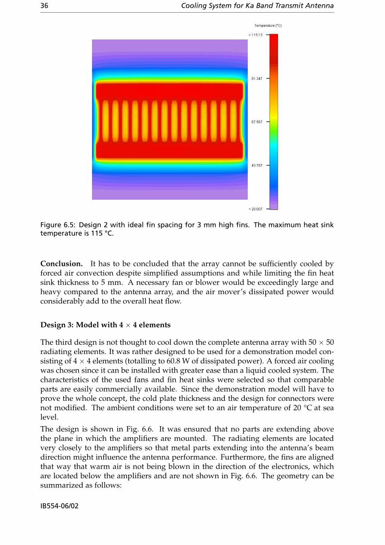
36 Cooling System for Ka Band Transmit Antenna
Figure 6.5: Design 2 with ideal fin spacing for 3 mm high fins. The maximum heat sinktemperature is 115 °C.
Conclusion. It has to be concluded that the array cannot be sufficiently cooled byforced air convection despite simplified assumptions and while limiting the fin heatsink thickness to 5 mm. A necessary fan or blower would be exceedingly large andheavy compared to the antenna array, and the air mover’s dissipated power wouldconsiderably add to the overall heat flow.
Design 3: Model with 4 × 4 elements
The third design is not thought to cool down the complete antenna array with 50 × 50radiating elements. It was rather designed to be used for a demonstration model con-sisting of 4 × 4 elements (totalling to 60.8 W of dissipated power). A forced air coolingwas chosen since it can be installed with greater ease than a liquid cooled system. Thecharacteristics of the used fans and fin heat sinks were selected so that comparableparts are easily commercially available. Since the demonstration model will have toprove the whole concept, the cold plate thickness and the design for connectors werenot modified. The ambient conditions were set to an air temperature of 20 °C at sealevel.
The design is shown in Fig. 6.6. It was ensured that no parts are extending abovethe plane in which the amplifiers are mounted. The radiating elements are locatedvery closely to the amplifiers so that metal parts extending into the antenna’s beamdirection might influence the antenna performance. Furthermore, the fins are alignedthat way that warm air is not being blown in the direction of the electronics, whichare located below the amplifiers and are not shown in Fig. 6.6. The geometry can besummarized as follows:
IB554-06/02

6. Cooling techniques 37
Figure 6.6: Design 3 for 4 × 4 elements. The fans have a side length of 50 mm each, theheat sink is 40 mm high.
Cold plate: The copper cold plate is 5 mm thick, 50 mm wide and 120 mm long. Thesquare part in the middle, on which the amplifiers are mounted, has a side lengthof 20 mm. The amplifiers and cut outs are positioned as shown in Fig. 3.3.
Extruded fin heat sink: The heat sinks are made out of aluminum and are 40 mm high.The fins are 38 mm long and 1 mm thick. The spacing between the fins equals2 mm.
Fan: The fan’s outer diameter is 50 mm, the hub diameter is 22 mm.2 The fans runat 5000 rounds per minute in a counter-clockwise direction as seen from above.They blow the air towards the heat sink and dissipate 2.52 W each (which wasincluded in the numerical simulation). The linearized version of the fan curvewith a free flow rate of 7.32 · 10−3 m3/s and a pressure drop at stagnation of18.9 Pa was taken into account.
Adhesive: The adhesive layer was assumed to be 0.25 mm thick. The thermal conduc-tivity was set to 1.05 W/(m K).3
The temperature distributions for two cross-sectional views are shown in Fig. 6.7. Thegeometries symmetry was exploited for the simulations to decrease computationaltime. This is why temperature distributions are not shown for the whole design. The
2The fan’s characteristics are based on the model F-520H12 S/C/B2 [39], which is available fromCofanUSA. Similar fans should lead to similar results.
3This data was based on the commercially available adhesive Elecolit® 6601 [40], distributed byPanacol-Elosol. The company could not provide data with respect to deterioration of thermal conduc-tivity over time.
IB554-06/02
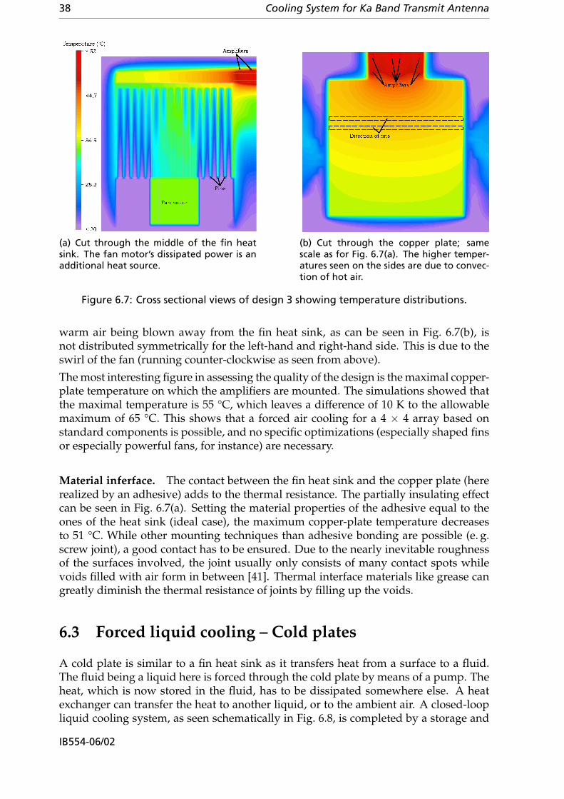
38 Cooling System for Ka Band Transmit Antenna
(a) Cut through the middle of the fin heatsink. The fan motor’s dissipated power is anadditional heat source.
(b) Cut through the copper plate; samescale as for Fig. 6.7(a). The higher temper-atures seen on the sides are due to convec-tion of hot air.
Figure 6.7: Cross sectional views of design 3 showing temperature distributions.
warm air being blown away from the fin heat sink, as can be seen in Fig. 6.7(b), isnot distributed symmetrically for the left-hand and right-hand side. This is due to theswirl of the fan (running counter-clockwise as seen from above).
The most interesting figure in assessing the quality of the design is the maximal copper-plate temperature on which the amplifiers are mounted. The simulations showed thatthe maximal temperature is 55 °C, which leaves a difference of 10 K to the allowablemaximum of 65 °C. This shows that a forced air cooling for a 4 × 4 array based onstandard components is possible, and no specific optimizations (especially shaped finsor especially powerful fans, for instance) are necessary.
Material inferface. The contact between the fin heat sink and the copper plate (hererealized by an adhesive) adds to the thermal resistance. The partially insulating effectcan be seen in Fig. 6.7(a). Setting the material properties of the adhesive equal to theones of the heat sink (ideal case), the maximum copper-plate temperature decreasesto 51 °C. While other mounting techniques than adhesive bonding are possible (e. g.screw joint), a good contact has to be ensured. Due to the nearly inevitable roughnessof the surfaces involved, the joint usually only consists of many contact spots whilevoids filled with air form in between [41]. Thermal interface materials like grease cangreatly diminish the thermal resistance of joints by filling up the voids.
6.3 Forced liquid cooling – Cold plates
A cold plate is similar to a fin heat sink as it transfers heat from a surface to a fluid.The fluid being a liquid here is forced through the cold plate by means of a pump. Theheat, which is now stored in the fluid, has to be dissipated somewhere else. A heatexchanger can transfer the heat to another liquid, or to the ambient air. A closed-loopliquid cooling system, as seen schematically in Fig. 6.8, is completed by a storage and
IB554-06/02

6. Cooling techniques 39
Expansion andstorage tank
Heat exchanger
Pump
Cold plate
Figure 6.8: Basic liquid cooling system.
expansion tank. Its purpose is to protect the system from increasing pressures due tothe expansion of the heated fluid, and to supply sufficient amounts of fluid to the loopat all times.
The general similarity to fin heat sinks is also expressed in the same equations, whichwere presented in Sec. 6.2. The basic improvement upon forced air cooling is the in-creased specific heat and thermal conductivity of liquid coolants as opposed to air. Thefluid flow rate and system size can be considerably reduced. Often, a liquid cooled sys-tem is less heavy and smaller than a comparable forced air cooling system despite theadded weight of pipes and coolant.
The main disadvantage of a liquid cooling system is the increased system complexity.Building a system which is sealed in all situations is more complicated (and expensive)than a forced air cooling system. Once fluid leaks out of the system, electronics can beelectrically (shorts), chemically (aggressive fluids), and thermally (hot fluid) destroyed.In the context of avionics, more effort is necessary to comply with security specifica-tions. This is certainly one reason why most avionics cooling systems are forced aircooling systems.
Another disadvantage of a liquid cold plate is that the array cannot be build modularwithout changing assembly constraints as indicated in Sec. 3.1. By modular, an arrayout of several sub-assemblies with, for instance, 4 × 4 elements is thought of. Thisis due to the fact that no feeding pipes can be mounted on the reverse side of thearray because of space considerations, and a sealed system would be very difficultto obtain for channels going through different sub-assemblies. A modular approachwould allow to individually fabricate and test sub-assemblies. In case of failure duringlater operation, not the whole array needed to be replaced. A modular approach wouldbecome possible by deviating from the assembly constraints. If components on thereverse side of the array could be arranged in a manner which allowed tube fittings, amodular approach might become possible.
A pump has to overcome flow resistance much the same way as fans have to workagainst the system resistance. The lower the flow resistance, the less pressure the pumphas to supply. This results in a smaller pump and therefore less dissipated pump power(which adds to the overall heat load). The causes for pressure drops in a liquid cooledsystem are:
• friction (depending on surface roughness and liquid velocity),
• elevation (if the liquid has to be pumped against gravity), and
• losses due to liquid guiding (elbows, transitions, etc.).
IB554-06/02

40 Cooling System for Ka Band Transmit Antenna
The third factor dominates for most systems. Pressure losses due to typical bends andtransitions are known; the same is true for various pipe entrances, where a roundedoff entry results in less pressure drop than a square edge entry, for instance [26].
Since an array size of 50 × 50 elements seems to be most likely at this stage of theproject, the development of a cold plate will be focused on this array size. Due to therepetitive structure of the array, similar results could be easily yielded in an analogousmanner for larger or smaller arrays.
6.3.1 Design considerations
Keeping in mind that the cold plate thickness is not to exceed 5 mm (see Sec. 3.1),it becomes apparent that liquid channels have to be oriented in parallel to the layercontaining the patches as shown in Fig. 3.2 on page 6.
The thermal resistance of the cold plate can be decreased by decreasing ∆TA and ∆TB
according to Eq. (6.4). Equation (6.5) indicates that ∆TA can be reduced by increasingthe mass flow rate m and by choosing a liquid with a high specific heat c. This sum-mand is correlated to the cold plate design by the flow resistance since a higher flowresistance yields a lower mass flow rate for a given pump.
The second summand, ∆TB, is described by Eq. (4.11). Therefore, the surface A and theheat transfer coefficient h should be as large as possible. The surface can be increasedby increasing the number of channels. This results in thinner channel walls and smallerchannel cross-sectional areas since the overall width of the array cannot be modified.This approach is limited by two factors: the wall width (since thin walls are morecomplicated to manufacture and are less mechanically stable), and the increased flowresistance (influencing ∆TA).
It is advantageous to build the cold plate out of one block of material since every mate-rial interface introduces another additional thermal resistance. Analogous to a foldedfin heat sinks for forced air cooling, the channels of the cold plate could be build out ofa folded thin layer of material. This would simplify machining as opposed to millingsuch a heat sink. The flow would be restricted by two cover plates, which are bondedto the channel structure.
The second factor determining ∆TB, the heat transfer coefficient h, is described by theNusselt number. Higher Nusselt numbers yield better heat transfer. As described inSec. 4.2.3, turbulent flow is therefore desired. Turbulent flow is more likely to occur forlarger channel diameters, higher fluid velocities, and lower kinematic viscosities (seeSec. 4.2.1). Assuming turbulent flow and combining Eqs. (4.3), (4.14), (4.17), (4.18),and (4.22), one yields the following function for the heat transfer coefficient:
h = 0.0235 · λ0.52(ρc)0.48
ν0.32· v0.8
d0.2. (6.15)
Therefore, the heat transfer coefficient increases for increasing
• thermal conductivity (fluid),
• density (fluid)
• specific heat (fluid),
• fluid flow velocity,
IB554-06/02
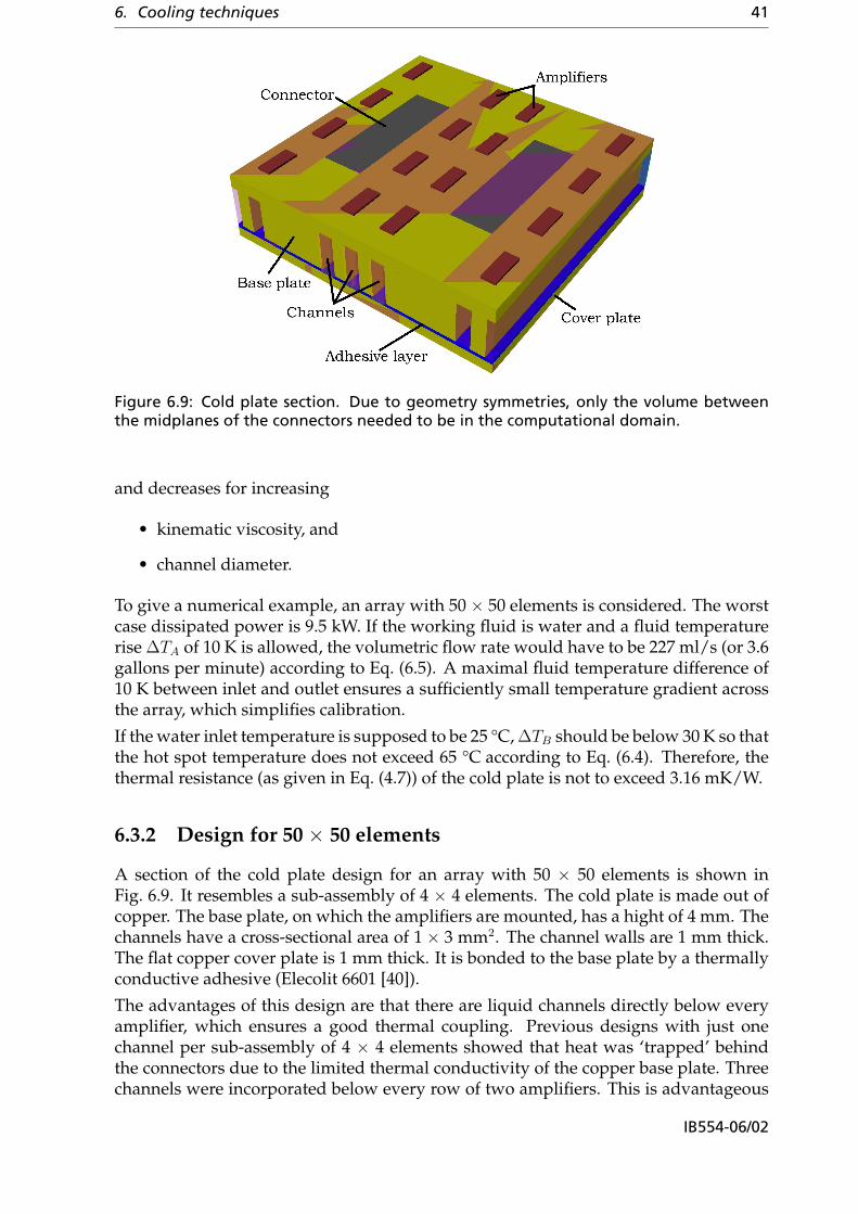
6. Cooling techniques 41
Figure 6.9: Cold plate section. Due to geometry symmetries, only the volume betweenthe midplanes of the connectors needed to be in the computational domain.
and decreases for increasing
• kinematic viscosity, and
• channel diameter.
To give a numerical example, an array with 50 × 50 elements is considered. The worstcase dissipated power is 9.5 kW. If the working fluid is water and a fluid temperaturerise ∆TA of 10 K is allowed, the volumetric flow rate would have to be 227 ml/s (or 3.6gallons per minute) according to Eq. (6.5). A maximal fluid temperature difference of10 K between inlet and outlet ensures a sufficiently small temperature gradient acrossthe array, which simplifies calibration.
If the water inlet temperature is supposed to be 25 °C, ∆TB should be below 30 K so thatthe hot spot temperature does not exceed 65 °C according to Eq. (6.4). Therefore, thethermal resistance (as given in Eq. (4.7)) of the cold plate is not to exceed 3.16 mK/W.
6.3.2 Design for 50 × 50 elements
A section of the cold plate design for an array with 50 × 50 elements is shown inFig. 6.9. It resembles a sub-assembly of 4 × 4 elements. The cold plate is made out ofcopper. The base plate, on which the amplifiers are mounted, has a hight of 4 mm. Thechannels have a cross-sectional area of 1 × 3 mm2. The channel walls are 1 mm thick.The flat copper cover plate is 1 mm thick. It is bonded to the base plate by a thermallyconductive adhesive (Elecolit 6601 [40]).
The advantages of this design are that there are liquid channels directly below everyamplifier, which ensures a good thermal coupling. Previous designs with just onechannel per sub-assembly of 4 × 4 elements showed that heat was ‘trapped’ behindthe connectors due to the limited thermal conductivity of the copper base plate. Threechannels were incorporated below every row of two amplifiers. This is advantageous
IB554-06/02
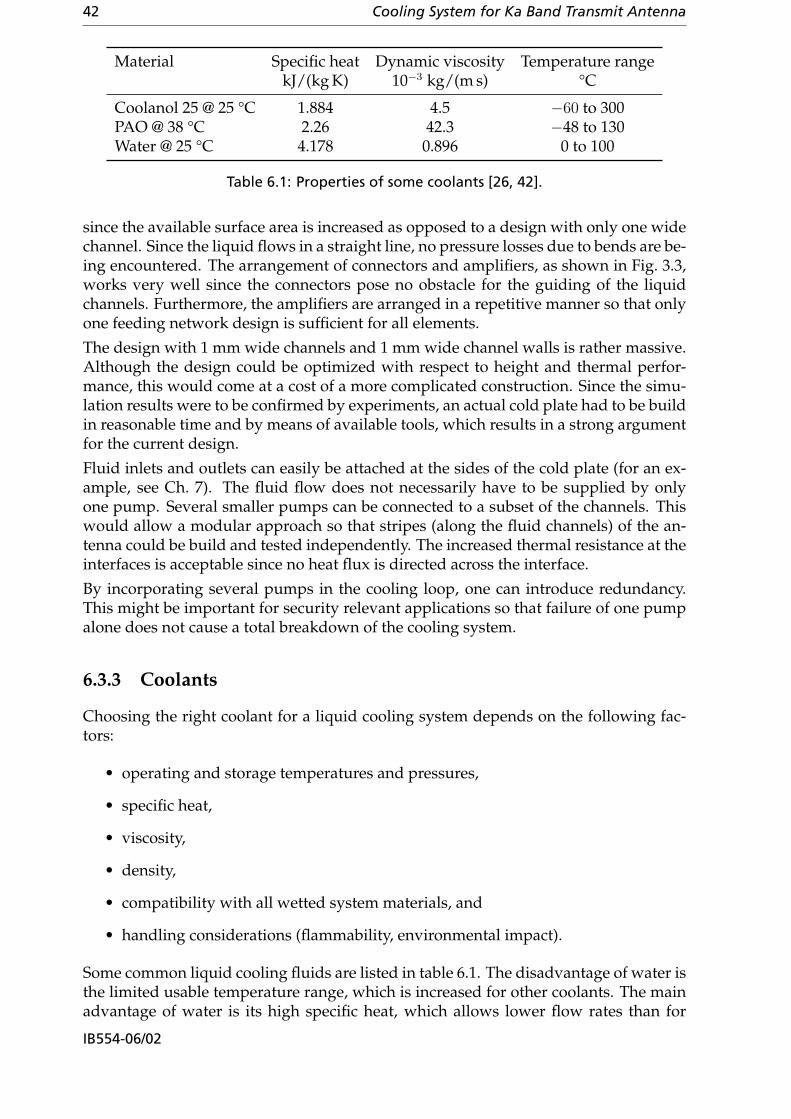
42 Cooling System for Ka Band Transmit Antenna
Material Specific heat Dynamic viscosity Temperature rangekJ/(kg K) 10−3 kg/(m s) °C
Coolanol 25 @ 25 °C 1.884 4.5 −60 to 300PAO @ 38 °C 2.26 42.3 −48 to 130Water @ 25 °C 4.178 0.896 0 to 100
Table 6.1: Properties of some coolants [26, 42].
since the available surface area is increased as opposed to a design with only one widechannel. Since the liquid flows in a straight line, no pressure losses due to bends are be-ing encountered. The arrangement of connectors and amplifiers, as shown in Fig. 3.3,works very well since the connectors pose no obstacle for the guiding of the liquidchannels. Furthermore, the amplifiers are arranged in a repetitive manner so that onlyone feeding network design is sufficient for all elements.
The design with 1 mm wide channels and 1 mm wide channel walls is rather massive.Although the design could be optimized with respect to height and thermal perfor-mance, this would come at a cost of a more complicated construction. Since the simu-lation results were to be confirmed by experiments, an actual cold plate had to be buildin reasonable time and by means of available tools, which results in a strong argumentfor the current design.
Fluid inlets and outlets can easily be attached at the sides of the cold plate (for an ex-ample, see Ch. 7). The fluid flow does not necessarily have to be supplied by onlyone pump. Several smaller pumps can be connected to a subset of the channels. Thiswould allow a modular approach so that stripes (along the fluid channels) of the an-tenna could be build and tested independently. The increased thermal resistance at theinterfaces is acceptable since no heat flux is directed across the interface.
By incorporating several pumps in the cooling loop, one can introduce redundancy.This might be important for security relevant applications so that failure of one pumpalone does not cause a total breakdown of the cooling system.
6.3.3 Coolants
Choosing the right coolant for a liquid cooling system depends on the following fac-tors:
• operating and storage temperatures and pressures,
• specific heat,
• viscosity,
• density,
• compatibility with all wetted system materials, and
• handling considerations (flammability, environmental impact).
Some common liquid cooling fluids are listed in table 6.1. The disadvantage of water isthe limited usable temperature range, which is increased for other coolants. The mainadvantage of water is its high specific heat, which allows lower flow rates than for
IB554-06/02
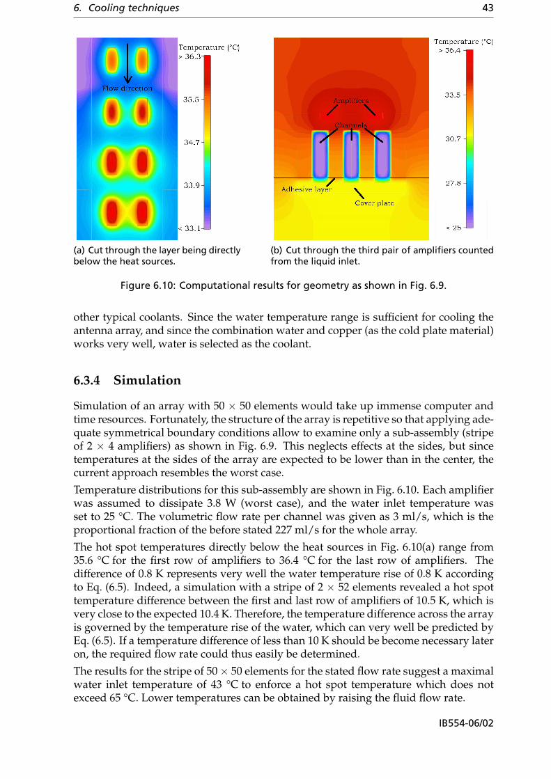
6. Cooling techniques 43
(a) Cut through the layer being directlybelow the heat sources.
(b) Cut through the third pair of amplifiers countedfrom the liquid inlet.
Figure 6.10: Computational results for geometry as shown in Fig. 6.9.
other typical coolants. Since the water temperature range is sufficient for cooling theantenna array, and since the combination water and copper (as the cold plate material)works very well, water is selected as the coolant.
6.3.4 Simulation
Simulation of an array with 50 × 50 elements would take up immense computer andtime resources. Fortunately, the structure of the array is repetitive so that applying ade-quate symmetrical boundary conditions allow to examine only a sub-assembly (stripeof 2 × 4 amplifiers) as shown in Fig. 6.9. This neglects effects at the sides, but sincetemperatures at the sides of the array are expected to be lower than in the center, thecurrent approach resembles the worst case.
Temperature distributions for this sub-assembly are shown in Fig. 6.10. Each amplifierwas assumed to dissipate 3.8 W (worst case), and the water inlet temperature wasset to 25 °C. The volumetric flow rate per channel was given as 3 ml/s, which is theproportional fraction of the before stated 227 ml/s for the whole array.
The hot spot temperatures directly below the heat sources in Fig. 6.10(a) range from35.6 °C for the first row of amplifiers to 36.4 °C for the last row of amplifiers. Thedifference of 0.8 K represents very well the water temperature rise of 0.8 K accordingto Eq. (6.5). Indeed, a simulation with a stripe of 2 × 52 elements revealed a hot spottemperature difference between the first and last row of amplifiers of 10.5 K, which isvery close to the expected 10.4 K. Therefore, the temperature difference across the arrayis governed by the temperature rise of the water, which can very well be predicted byEq. (6.5). If a temperature difference of less than 10 K should be become necessary lateron, the required flow rate could thus easily be determined.
The results for the stripe of 50× 50 elements for the stated flow rate suggest a maximalwater inlet temperature of 43 °C to enforce a hot spot temperature which does notexceed 65 °C. Lower temperatures can be obtained by raising the fluid flow rate.
IB554-06/02

44 Cooling System for Ka Band Transmit Antenna
To conclude, the presented cold plate meeting the dimension constraints is very wellable to cool down the antenna array. A total water flow rate of 227 ml/s at an inletwater temperature of about 25 °C for a 50 × 50 element array ensures a maximal tem-perature difference of 10 K across the array while keeping the hot spot temperature farbelow 65 °C.
6.3.5 Perspective
Improvements with respect to size and weight are possible, but they come at a cost ofa more complex design. A commercially available copper cold plate from Lytron, typeCP40 [43], features a plate thickness of 2.5 mm. Cut outs (for mounting components)are incorporated in the design, showing that they are generally possible. The coldplate contains crossed micro-channels. The advantage is turbulent liquid flow (betterheat transfer), but on the other hand, a resulting higher pressure drop requires a morepowerful pump.
6.4 Peltier coolers
A Peltier element (also called a thermoelectric converter or TEC) is a heat pump basedon the Peltier effect. By applying an electric current, one side heats up while the othercools down. Its main advantage is to be able to cool down a surface below ambienttemperature. As a cooling device, the cold side is attached to the heat source while thewarm side is connected to a heat sink (which is often a forced convection fin heat sink,but other heat sinks are possible as well). It’s main disadvantage is that the electriccurrent adds to the total heat load so that the heat sink has to dissipate more powerthan without a Peltier module. Depending on the specific characteristics of a design,a heat sink coupled to a Peltier element can therefore result in higher component tem-peratures than the heat sink by itself.
Geometrically, Peltier modules are flat plates where the two large surfaces heat up orcool down, respectively. If the cold plate in Fig. 3.2 were replaced by a Peltier element,the heat sink would have to be mounted where the circuit boards are placed. Thisrenders the elements unfit to cool down the antenna array since heat has to be removedto the sides.
6.5 Heat pipes
A heat pipe is able to transfer large amounts of heat in a two-phase flow system noise-less with no outside power at a very low temperature difference. A typical heat pipeconsists of a hollow, sealed metallic cylinder whose inner walls are covered with acapillary structure (called wick) as shown in Fig. 6.11. The tube is partly filled with aworking fluid. If the one end is heated up, the liquid evaporates and the vapor driftsdue to the pressure difference to the cold end. This condenser zone is connected to aheat sink by means of thermal conduction. The vapor condenses at the walls and trav-els back completing the circle to the heat source through the wick by means of capillaryaction.
Five limits exist which restrict the performance (power rating) of a heat pipe:
IB554-06/02
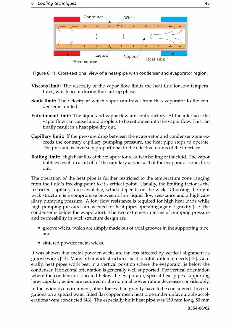
6. Cooling techniques 45
Heat sourceHeat sink
Wick
Liquid Vapour
Container
Figure 6.11: Cross-sectional view of a heat-pipe with condenser and evaporator region.
Viscous limit: The viscosity of the vapor flow limits the heat flux for low tempera-tures, which occur during the start-up phase.
Sonic limit: The velocity at which vapor can travel from the evaporator to the con-denser is limited.
Entrainment limit: The liquid and vapor flow are contradictory. At the interface, thevapor flow can cause liquid droplets to be entrained into the vapor flow. This canfinally result in a heat pipe dry out.
Capillary limit: If the pressure drop between the evaporator and condenser zone ex-ceeds the contrary capillary pumping pressure, the heat pipe stops to operate.The pressure is inversely proportional to the effective radius of the interface.
Boiling limit: High heat flux at the evaporator results in boiling of the fluid. The vaporbubbles result in a cut off of the capillary action so that the evaporator zone driesout.
The operation of the heat pipe is further restricted to the temperature zone rangingfrom the fluid’s freezing point to it’s critical point. Usually, the limiting factor is therestricted capillary force available, which depends on the wick. Choosing the rightwick structure is a compromise between a low liquid flow resistance and a high cap-illary pumping pressure. A low flow resistance is required for high heat loads whilehigh pumping pressures are needed for heat pipes operating against gravity (i. e. thecondenser is below the evaporator). The two extremes in terms of pumping pressureand permeability in wick structure design are
• groove wicks, which are simply made out of axial grooves in the supporting tube,and
• sintered powder metal wicks.
It was shown that metal powder wicks are far less affected by vertical alignment asgroove wicks [44]. Many other wick structures exist to fulfill different needs [45]. Gen-erally, heat pipes work best in a vertical position where the evaporator is below thecondenser. Horizontal orientation is generally well supported. For vertical orientationwhere the condenser is located below the evaporator, special heat pipes supportinglarge capillary action are required or the nominal power rating decreases considerably.
In the avionics environment, other forces than gravity have to be considered. Investi-gations on a special water filled flat copper mesh heat pipe under unfavourable accel-erations were conducted [46]. The especially built heat pipe was 150 mm long, 50 mm
IB554-06/02
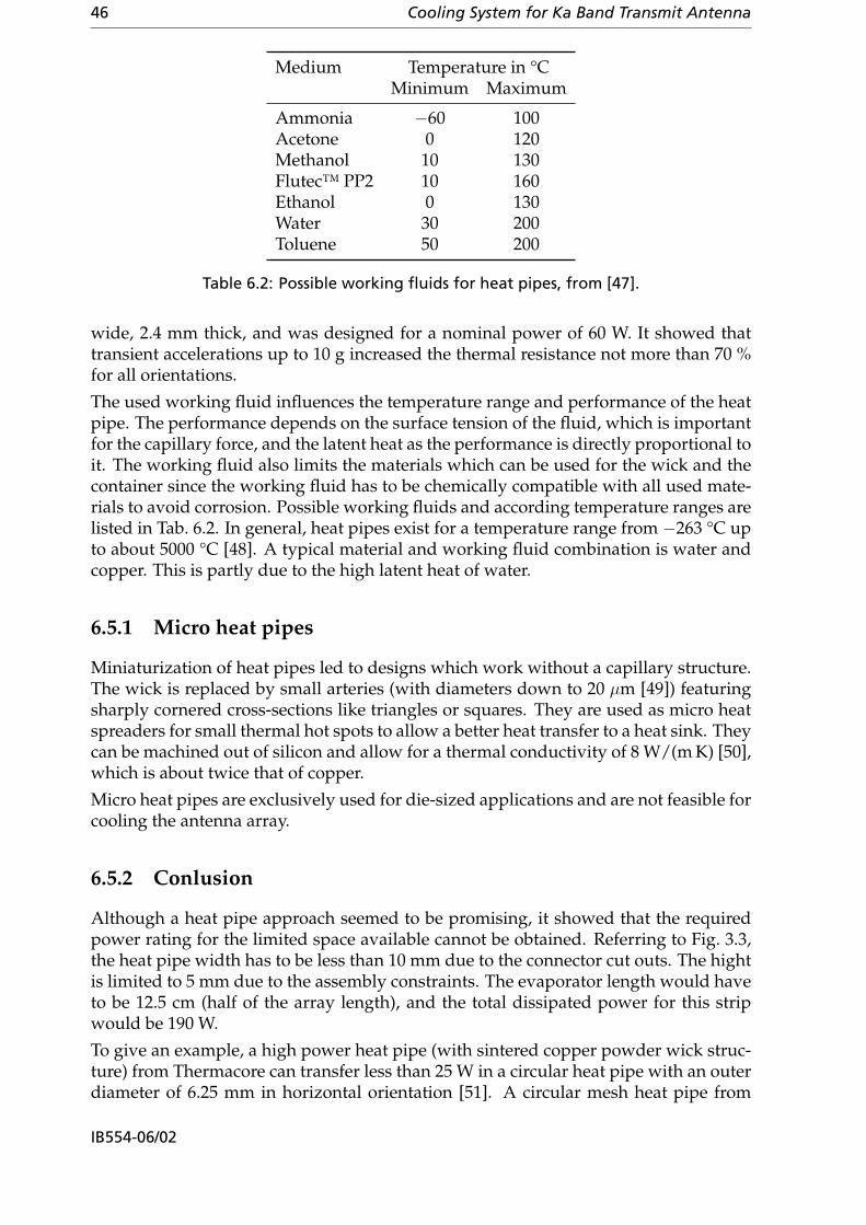
46 Cooling System for Ka Band Transmit Antenna
Medium Temperature in °CMinimum Maximum
Ammonia −60 100Acetone 0 120Methanol 10 130Flutec™ PP2 10 160Ethanol 0 130Water 30 200Toluene 50 200
Table 6.2: Possible working fluids for heat pipes, from [47].
wide, 2.4 mm thick, and was designed for a nominal power of 60 W. It showed thattransient accelerations up to 10 g increased the thermal resistance not more than 70 %for all orientations.
The used working fluid influences the temperature range and performance of the heatpipe. The performance depends on the surface tension of the fluid, which is importantfor the capillary force, and the latent heat as the performance is directly proportional toit. The working fluid also limits the materials which can be used for the wick and thecontainer since the working fluid has to be chemically compatible with all used mate-rials to avoid corrosion. Possible working fluids and according temperature ranges arelisted in Tab. 6.2. In general, heat pipes exist for a temperature range from −263 °C upto about 5000 °C [48]. A typical material and working fluid combination is water andcopper. This is partly due to the high latent heat of water.
6.5.1 Micro heat pipes
Miniaturization of heat pipes led to designs which work without a capillary structure.The wick is replaced by small arteries (with diameters down to 20 µm [49]) featuringsharply cornered cross-sections like triangles or squares. They are used as micro heatspreaders for small thermal hot spots to allow a better heat transfer to a heat sink. Theycan be machined out of silicon and allow for a thermal conductivity of 8 W/(m K) [50],which is about twice that of copper.
Micro heat pipes are exclusively used for die-sized applications and are not feasible forcooling the antenna array.
6.5.2 Conlusion
Although a heat pipe approach seemed to be promising, it showed that the requiredpower rating for the limited space available cannot be obtained. Referring to Fig. 3.3,the heat pipe width has to be less than 10 mm due to the connector cut outs. The hightis limited to 5 mm due to the assembly constraints. The evaporator length would haveto be 12.5 cm (half of the array length), and the total dissipated power for this stripwould be 190 W.
To give an example, a high power heat pipe (with sintered copper powder wick struc-ture) from Thermacore can transfer less than 25 W in a circular heat pipe with an outerdiameter of 6.25 mm in horizontal orientation [51]. A circular mesh heat pipe from
IB554-06/02
6. Cooling techniques 47
Quick-Ohm with an outer diameter of 6 mm is capable of transferring about 45 W [52].An inquiry at Atherm (a French company) confirmed that even a tailored heat pipeheat sink would not fulfill the required power rating.
6.6 Other cooling techniques
Expendable liquid systems. Expendable liquid systems are capable of dissipatinglarge heat loads. As an example it has been reported that the entire 23 kW heat loadin an aircraft was dissipated by means of an expendable liquid system [53]. The obvi-ous disadvantages of such a system are that refrigerants have to be refilled regularly.Therefore, they are not being considered for the given problem.
Micro-channel integrated heat sinks. Micro-channel heat sinks are cold plates fea-turing channels with a width in the micrometer range. Immense heat transfer ratescan be obtained; a reported heat flux of 790 W/cm2 for channel widths of 50 µm hasbeen dissipated for a total square area of 1 cm2 [54], to give an example. While thistechnology seems to be promising for modern high speed electronic circuits, where alarge amount of heat is dissipated locally, it is not suited for the given cooling problemof a distributed heat source with dimensions around 25 × 25 cm2.
Direct immersion cooling. Direct immersion cooling is principally very similar toair cooling. Now, the surrounding fluid, air, has been replaced by a liquid, which isoften a dielectric fluid. As for air cooling, several cooling methods can be consideredincluding natural and forced convection. See [55] for an overview. In addition to aircooling systems, two-phase flow can occur and heat transfer can be further increased.
Although this approach would allow to cool both the high frequency amplifiers andall other electronics by one cooling system, the technical challenge of building a sealedsystem and conditioning the fluid is far superior to a rather simple liquid cooled coldplate. Therefore, this approach is not being considered.
IB554-06/02


7 Experiments
The background behind conducting experiments was to verify the accuracy of simu-lation results especially with respect to the liquid cold plate as proposed in Sec. 6.3.2.Furthermore, it was thought to prove the feasibility of the before mentioned design,and to gain practical experience with liquid cold plates in general.
7.1 Design
The performance of the cold plate as described in Sec. 6.3.2 was to be confirmed byexperiments. Therefore, a simplified and downsized (less elements) model of the coldplate resembling the general geometry was built. This modified geometry, as shown inFig. 7.1, was simulated with Flotherm as well to allow a direct comparison of temper-ature values gained through experiments and simulations.
The built cold plate is shown in Fig. 7.1; detailed dimensions and pictures are givenin the Appendix in Fig. A.1 and A.2. The dimensions resemble an array with 12 ×10 elements. Three liquid channels with a cross-sectional area of 3 × 1 mm2 each arepositioned between each row of cut outs as well as to their sides (see Fig. A.2(a) fordetails). The connectors are realized as cut outs in the cold plate. Since tubes had tobe connected to the inlet and outlet of the cold plate, the cold plate was extended tosupport an adapter region. This was thought to provide better stability than two sepa-rate adapter regions, which would have to be connected to the middle block, althoughthe dimensions of the extensions are as large as the resembled array itself. The utilizedtubes had an inner diameter of 9.5 mm (3/8′′), which resulted in a rather large tubefitting. Comparing the cross-sectional areas of the tube (70.9 mm2) and the total cross-sectional area of all 15 channels (45 mm2), it becomes apparent that the cold plate actsas a flow resistance. The tube fitting was connected to the cold plate by means of ascrew joint, which was detachably sealed by an adhesive.
The actual cold plate (with thickness 4 mm) featuring the milled channels was madeout of copper. The cover plate (with thickness 1 mm) was instead made out of brassdue to better machining properties of this material. The cover plate and the aluminumscrew nut blocks were permanently attached to the copper base plate by means of athermally conductive adhesive (Elecolit 6601).
Resistors as heat sources. The main heat sources for the antenna array are the am-plifiers. They were replaced by (cheap) SMD resistors. The amplifiers have a maxi-mal power dissipation of 3.8 W, and their size is 2.44 × 1.15 mm2. There are no SMDresistors commercially available which could cope with such a high power rating fea-turing such a small footprint. A compromise had to be found, and chip resistors (typePWC) from Welwyn were finally selected [56]. They feature a power rating of 1.5 W at
49

50 Cooling System for Ka Band Transmit Antenna
Figure 7.1: Built cold plate; the heat sources are located on the reverse side. It consistsof four parts: copper base plate, brass cover plate, and two aluminum blocks featuringscrew threads for the tube fittings. Dimensions are shown in Fig. A.1 in the Appendix.
70 °C base plate temperature, occupying a footprint area of 6.5 × 3.2 mm2.
One resistor alone already exceeds the area available for one element (of 5 × 5 mm2).Since additional space was needed for circuit paths, one resistor finally representedfour amplifiers. In total, 30 resistors, with a resistance of 220 Ω (2 %) each, representedtherefore 120 amplifiers. One terminal of each resistor was soldered to a printed circuitboard (0.2 mm thick, material: FR-4). The other terminal was directly soldered to thecopper cold plate, which was utilized as ground. The solder (λ ≈ 50 W/(m K)) wasthought to provide good thermal coupling to the cold plate.
The positions of the resistors and the layout of the printed circuit board can be see inFig. A.3 in the Appendix. The circuit board was bonded to the copper cold plate bymeans of a thermally conductive adhesive (Elecolit 6601). The same adhesive was usedto attach the resistors to the circuit board prior to soldering.
7.2 Thermometer
The used thermometer is the DTM 3080 from LKM electronic [57]. It allows for tem-perature measurements in the range from −200 . . . 820 °C with an accuracy of 0.1 °C.The utilized temperature sensor is the WTF30 spring loaded tip surface probe from thesame company. The approximately circular surface area has a diameter of 2.5 mm. Itis a class A Pt100 sensor according to DIN EN 60751, which allows for an accuracy ofat least 0.5 K in the interesting temperature range (0 . . . 150 °C). The sensor operatingrange is −50 . . . 400 °C.
A resistance temperature detector (RTD) based thermometer was chosen as opposedto a thermocouple based one due to the higher accuracy achievable. The accuracy ofthermocouples is usually not better than 0.75 % of the temperature for the complete
IB554-06/02

7. Experiments 51
Inlet Outlet1 2
34 5
67 8
Circuit pathResistor PCB
Copper
Figure 7.2: Location of measurement points; view from above.
temperature range. RTDs suffer from a slower response time as opposed to thermo-couple probes, which is not of major concern for static measurements.
Practical experience. It showed that surface measurements are difficult to performsince the surface probe is not immersed into the object. The flat probe tip had to be verywell aligned with the (equally flat) surface under consideration. Very slight changes inalignment resulted in supposedly random temperature steps up to 10 K for measure-ments at around 70 °C. Reproducible results were not obtainable on uneven surfaceslike soldering joints. The use of thermal grease did not improve the predictability ofresults.
Therefore, a supporting stand for the probe was manufactured in order to enforce aprecisely upright orientation of the probe. It was made out of a 50 mm thick plasticblock, in which several drilled holes defined the positions of the probe. The so definedpositions are indicated in Fig. 7.2. This new approach worked very well for all pointsexcept number 4 and 5 (measurement directly at the surface of a resistor). For these twopoints, by merely turning the probe slightly around its axis, temperature differences ofup to 10 K were obtained. This was attributed to two factors: First, the flat area atthe probe tip is not exactly orthogonally aligned with respect to the probe axis. Thisslight misalignment results in a thermal interface which is based on a few contact spotsonly. The second factor is the high temperature gradient across the resistor surface. Byturning the probe, the contact spot was moved along the surface which explains theunreproducible temperature values. Therefore, the temperature values from the spotsnumber 4 and 5 were left out in the discussion of results.
7.3 Experimental setup and execution
Fluid flow. Distilled water was used as the coolant. It was chosen due to its goodavailability and high specific heat.
The hot spot temperature of the cold plate depends on the liquid flow rate, which hadto be measured. Since no flowmeter was available, the volumetric flow rate was gainedby measuring the liquid volume which flowed through the cold plate in a certain time.For that, the closed-loop system as shown in Fig. 6.8 was transferred to an open loopsystem.
A constant flow rate was necessary to perform the temperature measurements for thevarious measurement spots. The first approach utilized a direct current pump (type
IB554-06/02
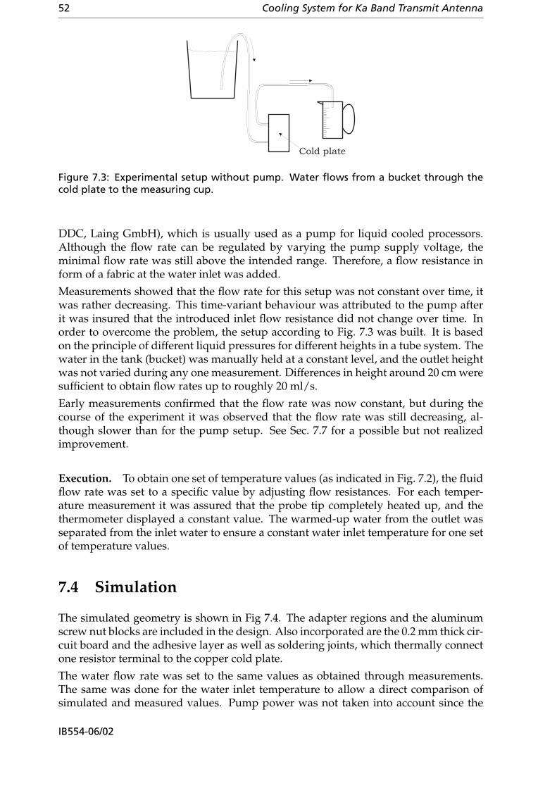
52 Cooling System for Ka Band Transmit Antenna
Cold plate
Figure 7.3: Experimental setup without pump. Water flows from a bucket through thecold plate to the measuring cup.
DDC, Laing GmbH), which is usually used as a pump for liquid cooled processors.Although the flow rate can be regulated by varying the pump supply voltage, theminimal flow rate was still above the intended range. Therefore, a flow resistance inform of a fabric at the water inlet was added.
Measurements showed that the flow rate for this setup was not constant over time, itwas rather decreasing. This time-variant behaviour was attributed to the pump afterit was insured that the introduced inlet flow resistance did not change over time. Inorder to overcome the problem, the setup according to Fig. 7.3 was built. It is basedon the principle of different liquid pressures for different heights in a tube system. Thewater in the tank (bucket) was manually held at a constant level, and the outlet heightwas not varied during any one measurement. Differences in height around 20 cm weresufficient to obtain flow rates up to roughly 20 ml/s.
Early measurements confirmed that the flow rate was now constant, but during thecourse of the experiment it was observed that the flow rate was still decreasing, al-though slower than for the pump setup. See Sec. 7.7 for a possible but not realizedimprovement.
Execution. To obtain one set of temperature values (as indicated in Fig. 7.2), the fluidflow rate was set to a specific value by adjusting flow resistances. For each temper-ature measurement it was assured that the probe tip completely heated up, and thethermometer displayed a constant value. The warmed-up water from the outlet wasseparated from the inlet water to ensure a constant water inlet temperature for one setof temperature values.
7.4 Simulation
The simulated geometry is shown in Fig 7.4. The adapter regions and the aluminumscrew nut blocks are included in the design. Also incorporated are the 0.2 mm thick cir-cuit board and the adhesive layer as well as soldering joints, which thermally connectone resistor terminal to the copper cold plate.
The water flow rate was set to the same values as obtained through measurements.The same was done for the water inlet temperature to allow a direct comparison ofsimulated and measured values. Pump power was not taken into account since the
IB554-06/02
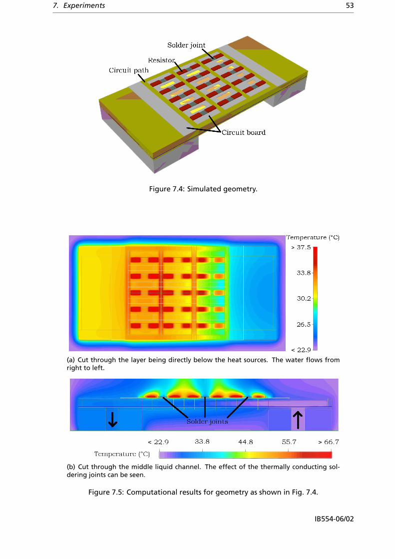
7. Experiments 53
Figure 7.4: Simulated geometry.
(a) Cut through the layer being directly below the heat sources. The water flows fromright to left.
(b) Cut through the middle liquid channel. The effect of the thermally conducting sol-dering joints can be seen.
Figure 7.5: Computational results for geometry as shown in Fig. 7.4.
IB554-06/02
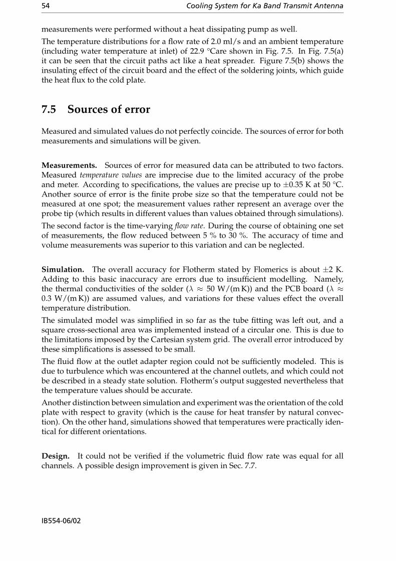
54 Cooling System for Ka Band Transmit Antenna
measurements were performed without a heat dissipating pump as well.
The temperature distributions for a flow rate of 2.0 ml/s and an ambient temperature(including water temperature at inlet) of 22.9 °Care shown in Fig. 7.5. In Fig. 7.5(a)it can be seen that the circuit paths act like a heat spreader. Figure 7.5(b) shows theinsulating effect of the circuit board and the effect of the soldering joints, which guidethe heat flux to the cold plate.
7.5 Sources of error
Measured and simulated values do not perfectly coincide. The sources of error for bothmeasurements and simulations will be given.
Measurements. Sources of error for measured data can be attributed to two factors.Measured temperature values are imprecise due to the limited accuracy of the probeand meter. According to specifications, the values are precise up to ±0.35 K at 50 °C.Another source of error is the finite probe size so that the temperature could not bemeasured at one spot; the measurement values rather represent an average over theprobe tip (which results in different values than values obtained through simulations).
The second factor is the time-varying flow rate. During the course of obtaining one setof measurements, the flow reduced between 5 % to 30 %. The accuracy of time andvolume measurements was superior to this variation and can be neglected.
Simulation. The overall accuracy for Flotherm stated by Flomerics is about ±2 K.Adding to this basic inaccuracy are errors due to insufficient modelling. Namely,the thermal conductivities of the solder (λ ≈ 50 W/(m K)) and the PCB board (λ ≈0.3 W/(m K)) are assumed values, and variations for these values effect the overalltemperature distribution.
The simulated model was simplified in so far as the tube fitting was left out, and asquare cross-sectional area was implemented instead of a circular one. This is due tothe limitations imposed by the Cartesian system grid. The overall error introduced bythese simplifications is assessed to be small.
The fluid flow at the outlet adapter region could not be sufficiently modeled. This isdue to turbulence which was encountered at the channel outlets, and which could notbe described in a steady state solution. Flotherm’s output suggested nevertheless thatthe temperature values should be accurate.
Another distinction between simulation and experiment was the orientation of the coldplate with respect to gravity (which is the cause for heat transfer by natural convec-tion). On the other hand, simulations showed that temperatures were practically iden-tical for different orientations.
Design. It could not be verified if the volumetric fluid flow rate was equal for allchannels. A possible design improvement is given in Sec. 7.7.
IB554-06/02

7. Experiments 55
252627282930313233
0 2 4 6 8Volumetric flow rate (in ml/s)
Tem
pera
ture
(in
°C
) MeasurementSimulation
(a) Measuring point 3 (circuit path, inlet).
2728293031323334353637
0 2 4 6 8Volumetric flow rate (in ml/s)
Tem
pera
ture
(in
°C
) MeasurementSimulation
(b) Measuring point 6 (circuit path, outlet).
20
21
22
23
24
25
26
27
0 2 4 6 8Volumetric flow rate (in ml/s)
Tem
pera
ture
(in
°C
) MeasurementSimulation
(c) Measuring point 2 (PCB, inlet).
2122232425262728293031
0 2 4 6 8Volumetric flow rate (in ml/s)
Tem
pera
ture
(in
°C
) MeasurementSimulation
(d) Measuring point 7 (PCB, outlet).
Figure 7.6: Comparison of experimental and simulation results; numbering according toFig. 7.2. Error bars represent Flotherm’s accuracy of ±2 K.
7.6 Results and discussion
Since the water inlet temperature was not the same for all measurements, all valueswere shifted to reflect a constant water inlet temperature of 20 °C. This allows for directcomparison of all temperature values.
The comparison between measurement and simulation are shown in Fig. 7.6 for mea-suring points 2, 3, 6, and 7. The values for measuring points 4 and 5 (directly on theresistors) were discarded due to effects described in Sec. 7.2. The graphs include errorbars (±2 K), which indicate the accuracy of Flotherm. It can be seen that except forone value in Fig. 7.6(b) all measured temperature values lie within this accuracy. Ifone would indicate the error bars for the measurement values as well (at least ±0.35 Kdue to the thermometer accuracy neglecting other effects), it becomes apparent thatcoherent results were obtained for all values.
The shape of the curves complies with theory. For flow rates from 2 ml/s to 6.85 ml/s,the Reynolds number ranges from 74 to 255, assuming the same volumetric flow ratesthrough each channel. This indicates laminar flow. For laminar flow, the heat transferdoes not depend on the flow rate, which would influence ∆TB in Eq. (6.4). On theother hand, ∆TA according to the same equation is inversely proportional to the massflow rate, explaining the hyperbolic shape.
It can be concluded that the accuracy of Flotherm for this computational model is atleast ±2 K. This supports the choice of Flotherm as the computational tool. Since the
IB554-06/02

56 Cooling System for Ka Band Transmit Antenna
geometry resembles quite closely the one of the proposed cold plate for an array with50 × 50 elements (see Sec. 6.3.2), it can be justifiably assumed that these simulationresults are accurate up to ±2 K as well.
Practical experience. The practical experience with the liquid cold plate was positivethroughout the project. It could be manufactured without special tools in a reasonabletime. No liquid leakage occurred whatsoever. The cold plate made a very robust im-pression which allows the cold plate to be used as a mechanical support for the antennaarray as well.
7.7 Improvements
Although the definite cause for the decreasing liquid flow rate could not be found, itseems to be possible that the (slow) liquid flow was obstructed by accumulated airin the system and especially by air bubbles in the small liquid channels. This couldexplain the gradual decrease of the flow rate and the increase after the system hadbeen at rest for a while.
To prove this point, a transparent cover plate (e. g. glass, acrylic glass) could replace thebrass plate to allow observation of the liquid flow. By this approach and using coloredwater, it could be as well examined if the fluid velocity in the channels is uniform forall channels (as is suggested by simulations). Since the brass plate was permanentlyattached (by means of adhesive) to the cold plate, this approach could not be followedduring the course of this project.
IB554-06/02
8 Heat exchanger
At this stage of the ATENAA project investigations have been directed towards show-ing that an Ka band antenna array could generally be build. Detailed analysis of a laterinstallation was excluded so far, and that is why the development of the cooling sys-tem concentrated simply on heat extraction rather than the development of a completecooling loop as shown in Fig 6.8. Nevertheless, the heat exchanger is an important partof a closed loop liquid cooling system as proposed in Sec. 6.3 so that general ideas willbe presented here.
The heat exchanger has to ensure that the warm water is sufficiently cooled down be-fore it enters the cold plate again. A typical approach of dissipating heat in aviationelectronics is by means of air cooling. Cool air is supplied by the aircraft’s environmen-tal control system (ECS). The worst-case total dissipated power of all power amplifiers(not including other electronics) for a 50× 50 element array is 9.5 kW, which adds con-siderable to the heat load for the ECS. If an air-cooled heat exchanger is used, it has tobe ensured that the ECS can cope with the added head load.
To give an idea of the required heat exchanger size, a commercially available air cooledheat exchanger was selected as an example. The selection was based on the followingassumptions:
• maximum heat load of 9.5 kW,
• air inlet temperature of 20 °C,
• fluid is water,
• water inlet temperature of 55 °C, and
• water flow rate of 0.125 l/s.
A heat exchanger from Lytron, type 6340, meets the requirements [43]. The thermal re-sistance is 280.5 W/K at a liquid flow rate of 0.125 l/s. The outer dimensions (excludingfans) are 630 × 564 × 89 mm3. The recommended fan type (four fans are needed forthis heat exchanger) is from Comair Rotron, type Caravel, which adds another 89 mm(totalling to 178 mm) to the overall height of the complete heat sink. This simple exam-ple shows that heat exchanger dimensions are still reasonable considering the cabinetsize constraint of 2 × 1 × 0.3 m2 as defined by the ATENAA project. Nevertheless, theheat exchanger takes up valuable space.
An advantage of a liquid cooled system is that heat (i. e. the warm liquid) can easily betransfered over a longer distance. It would be possible to exclude the heat sink fromthe cabinet in which the complete antenna module is mounted.
Another approach to heat rejection than air cooling is to transfer heat to the aircraftfuel [34]. This cooling method and its correlated problems are very specific to theactual aicraft and beyond the scope of this work.
57

58 Cooling System for Ka Band Transmit Antenna
In order to lower the heat load on the environmental control system, a heat sink basedon expendable coolants could be used [34]. The principle is that a high amount of heatcan be dissipated due to the latent heat of a coolant. The evaporated medium is thendisposed to the outside of the aircraft. The disadvantages are that additional mass hasto be transported, and that the cooling system has to be regularly refilled. Therefore,this scheme is not likely to be incorporated into commercial aircrafts.
IB554-06/02

9 Conclusion
The question under consideration was if a cooling system for an active antenna arrayin the Ka band could be developed. Several cooling technologies including forced airand liquid cooling as well as heat pipe cold plates were examined.
Forced air cooling systems are not able to cope with the high heat load of a full-sizedantenna array given the assembly constraints. Nevertheless, a forced convection finheat sink based on standard components was proposed for an array of 4 × 4 elements(see Sec. 6.2.2). This can be used as a cooling system for an antenna demonstrationmodel.
Although heat pipes are a promising approach for many applications due to their highheat transfer capabilities and a passive, sealed system, the required heat loads couldnot be transfered (see Sec. 6.5). This resulted from assembly constraints which limitedthe highest possible cross-sectional area of the heat pipes.
Simulations using Flotherm showed that a liquid cold plate is very well suited to ful-fill all requirements (see Sec. 6.3). A worst case heat load of 9.5 kW for an array of50 × 50 elements can be dissipated. Experiments on a simplified (i. e. smaller) modelconfirmed the practical feasibility of the cold plate (see Ch. 7). Comparison of mea-surements and simulations showed good agreement between both, which reinforcedthe decision to use the stated software.
59


A Detailed drawings and pictures ofcold plate
On the following pages, detailed drawings and pictures of the built cold plate areshown.
61
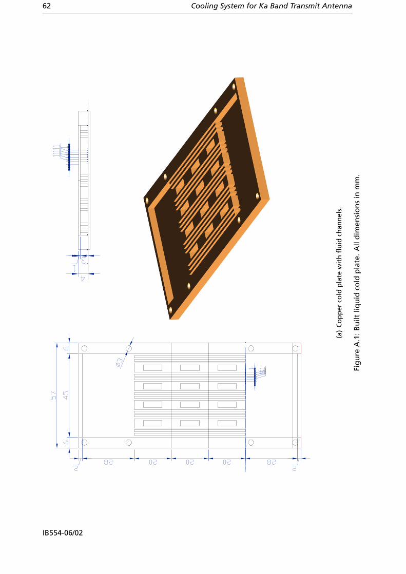
62 Cooling System for Ka Band Transmit Antenna
(a)
Co
pp
erco
ldp
late
wit
hfl
uid
chan
nel
s.
Fig
ure
A.1
:B
uilt
liqu
idco
ldp
late
.A
lld
imen
sio
ns
inm
m.
IB554-06/02

A. Detailed drawings and pictures of cold plate 63
(b)
Bra
ssco
ver
pla
te.
Fig
ure
A.1
:B
uilt
liqu
idco
ldp
late
.
IB554-06/02
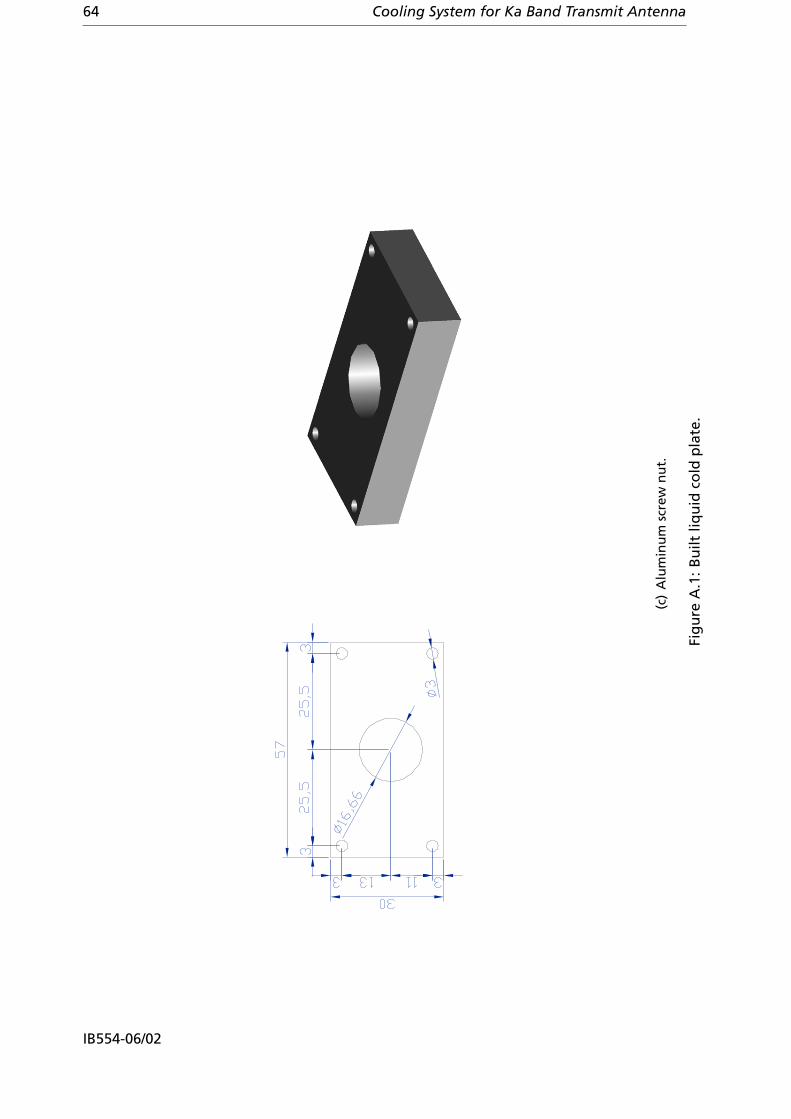
64 Cooling System for Ka Band Transmit Antenna
(c)
Alu
min
um
scre
wn
ut.
Fig
ure
A.1
:B
uilt
liqu
idco
ldp
late
.
IB554-06/02

A. Detailed drawings and pictures of cold plate 65
(a) Copper base plate featuring channels.
(b) Complete cold plate including inlet and outlet. The heat sources (resistors) are locatedon the reverse side.
Figure A.2: Picture of the build cold plate. The cut outs resemble the positions of theconnectors.
IB554-06/02

66 Cooling System for Ka Band Transmit Antenna
10,0
0
10,0
63,0
10,0
3,0
7,0
10,06,2
13,8
18,4
44,5
6,2
Fräsvorlage (2:1)14. November 2005
5,7
57,00
Alle Längen in mm
Milled out region
Circuit path
Resistor
Figure A.3: Circuit board for built liquid cold plate. The 0.2 mm thick substrate was milledto allow one terminal of each resistor to be soldered directly to the copper base plate.
IB554-06/02

Bibliography
[1] Christian Hunscher, Michael Thiel, Achim Dreher, Sybille Holzwarth, Leif C.Stange, Holger Pawlak, Alexander Molke, and Arne F. Jacob. SANTANA – Smartantenna terminal, final report. Technical report, EADS Astrium, DLR, IMSTGmbH, and TU Braunschweig, 2004.
[2] RTCA, Inc., Washington, DC. RTCA/DO-160D. Environmental Conditions and TestProcedures for Airborne Equipment, July 1997.
[3] Normenstelle Luftfahrt im DIN Deutsches Insitut für Normung e. V. DIN ISO2533: Normatmosphäre, December 1979.
[4] H. Zeffert. Principles and Practice of Aircraft Electrical Engineering. George NewnesLimited, London, 1960.
[5] Maximilian Wutz. Wärmeabfuhr in der Elektronik. Vieweg, 1991.
[6] Joe Yoon. Concorde history II. Retrieved September 29, 2005 from the World WideWeb: http://www.aerospaceweb.org/question/planes/q0199.shtml,2004.
[7] TriQuint Semiconductor 27–31 GHz 1 W power amplifier TGA4509-EPU datasheet, January 2005.
[8] Iridium Corporation of America. Eutectic Gold/Tin Solder. Product Data Sheet, 2005.
[9] Dwight E. Gray, editor. American Institute of Physics Handbook. McGraw-Hill, sec-ond edition, 1963.
[10] S. I. Novikova. Investigation of thermal expansion of GaAs and ZnSe. In John S.Blakemore, editor, Gallium Arsenide. American Insitute of Physics, Original articlesubmitted June 13, 1960. Reprinted from Soviet Physics – Solid State, vol. 3, (1961).
[11] Mark Occhionero, Richard Adams, and Kevin Fennessy. A new substrate for elec-tronic packaging: Aluminum-silicon carbide (AlSiC) composites. In Proceedingsof the Forth Annual Portable by Design Conference, Electronics Design, pages 398–403,March 1997.
[12] David L. Saums. Developments in selective high thermal conductivity orientationin CTE-compatible substrate and package component materials. In SemiconductorThermal Measurement and Management Symposium, March 2004.
[13] Jeanne Pavio and Don Hyde. Effects of coefficient of thermal expansion mismatchon solder attached GaAs MMICs. In IEEE Microwave Symposium Digest, volume 3,June 1991.
67

68 Cooling System for Ka Band Transmit Antenna
[14] Tom Tuhus and Are Bjorneklett. Thermal cycling reliability of die bonding adhe-sives. In International Reliability Physics Symposium, March 1993.
[15] Horst Stöcker, editor. Taschenbuch der Physik. Verlag Harri Deutsch, Thun andFrankfurt am Main, third edition, 1998.
[16] Wolfgang Beitz and Karl-Heinz Küttner, editors. Taschenbuch fü den Maschinenbau/ Dubbel. Springer, 17th edition, 1990.
[17] Massachuchetts Institute of Technology OpenCourseWare. Retrievedfrom the World Wide Web November 2, 2005: http://ocw.mit.edu/NR/rdonlyres/Materials-Science-and-Engineering/3-11Mechanics-of-MaterialsFall1999/698ECA59-8F00-46CC-96A1-B9365CBD63E3/0/props.pdf, 1999.
[18] Collaboration. Authors and Editors of the LB Volumes III/17A-22A-41A1b. Gal-lium arsenide (GaAs), Debye temperature, density, heat capacity, melting point, vol-ume 41. Subvolume A1A/2001 of Landolt-Börnstein - Group III Condensed Matter.Springer-Verlag GmbH, January 2001.
[19] GaAs MMIC ESD, Die Attach and Bonding Guidelines, May 2000. Agilent Technolo-gies, Application Note no. 54 – Rev. A.
[20] Klaus Langenheinecke, editor. Thermodynamik für Ingenieure. Viewegs Fachbücherder Technik, 1993.
[21] Ulrich Grigull and Heinrich Sandner. Wärmeleitung. Springer-Verlag, Berlin, 1979.
[22] Klaus Gersten. Einführung in die Strömungsmechanik. Verlag Vieweg, sixth edition,1991.
[23] Walter Wagner. Wärmeübertragung. Kamprath-Reihe. Vogel Buchverlag, third edi-tion, 1991.
[24] Erich Truckenbrodt. Lehrbuch der angewandten Fluidmechanik. Springer-Verlag,1983.
[25] U. Grigull, H. Sandner, J. Straub, and H. Winkler. Origins of dimensionless groupsof heat and mass transfer. Retrieved from the World Wide Web on December9, 2005: http://www.ichmt.org/dimensionless/dimensionless.html,1982. On the occasion of the 7th interational Heat Transfer Conference, München.
[26] Dave S. Steinberg. Cooling Techniques for Electronic Equipment. A Wiley-IntersciencePublication. John Wiley & Sons, 1980.
[27] McCarthy. Convective heat transfer example. Retrieved from the World WideWeb December 9, 2005: http://granular.che.pitt.edu/~mccarthy/che1011/Intro/Conv/conv_a.html.
[28] Hans Dieter Baehr and Karl Stephan. Wärme- und Stoffübertragung. Springer-Verlag, 1994.
[29] User’s Manual. Thermal Desktop – A CAD based system for Thermal analysis and De-sign. Version 4.7, Patch 3., October 2004.
IB554-06/02

BIBLIOGRAPHY 69
[30] David A. Johnson, Mark J. Welch, and Brent A. Cullimore. Novel simulation tech-niques for design of air-cooled electronics. In Proceedings of InterPack ’01, July2001.
[31] Flomerics Limited, Surrey, England. Getting Started with FLOTHERM – For softwareversion 5.1.
[32] Robin Bornoff. Validation of localized grid in version 4.2. Technical report, Flom-erics Ltd., November 2003.
[33] Christopher Hess. Technology for the good climate on board. Flug Review, October1999.
[34] P. W. Smith, editor. Avionic Cooling and Power Supplies for Advanced Aircraft. NorthAltantic Treaty Organization. Advisory Group for Aerospace Research and Devel-opment, June 1976.
[35] Maik Turner. All you need to know about fans. Electronics Cooling, 2(2), May 1996.
[36] C. L. Belady. Design considerations for air cooling electronic systems in high al-titude conditions. IEEE Transactions on Components, Packaging, and ManufacturingTechnology, 19(4), 1996.
[37] James Edwin Marthinuss Jr. and George Thomas Hall. Cooling electronics at highaltitudes made easy. Electronics Cooling, 4(3), 1998.
[38] PTI Pelonis Technologies, Inc. DC Blower 1230, 2005.
[39] CofanUSA, Fremont, CA. DC Brushless Fan Motor – 50 * 50 * 20 mm. Retrievedfrom the WWW on November 20, 2005: http://www.cofan-usa.com/New/fans/dc_fans/50x20/50x20.PDF.
[40] Panacol-Elosol GmbH. Elecolit® 6601. Technisches Datenblatt.
[41] L. S. Fletcher. A review of thermal enhancement techniques for electronic systems.In InterSociety Conference on Thermal Phenomena in Electronic Systems, May 1990.
[42] Rf dummy loads, calorimeters and cooling equipment for electronics, catalog2000.
[43] Lytron. Lytron – Total Thermal Solutions, 2004 Catalog, 2004.
[44] C. K. Loh, Enisa Harris, and D. J. Chou. Comparative study of heat pipes per-formances in different orientations. In Semiconductor Thermal Measurement andManagement Symposium, pages 191–195. IEEE, March 2005.
[45] Adrian Bejan and Allan D. Kraus. Heat Transfer Handbook. John Wiley & Sons, Inc.,2003.
[46] Mohamed Chaker Zaghdoudi, Christian Tantolin, and Claude Godet. Flat heatpipes thermal performance in body force environment. In Inter Society Conferenceon Thermal Phenomena, 2000.
[47] Shankara Narayanan K.R. What is a heat pipe. Retrieved from the WorldWide Web November 28, 2005: http://www.cheresources.com/htpipes.shtml.
IB554-06/02

70 Cooling System for Ka Band Transmit Antenna
[48] Beate Unger. 10 wichtige regeln für die verwendung von heatpipes. Retrievedfrom the World Wide Web November 30, 2005: http://www.quick-cool-waermetransfer.de/heatpipe/download/10-Regeln_Heatpipe.pdf.
[49] C. B. Sobhan. Miniaturization: Modern trends in heat pipe technology. Retrievedfrom the World Wide Web November 26, 2005: file:///H:/docs/cooling-techniques/heat-pipes/Miniaturization%20Modern%20Trends%20in%20Heat%20Pipe%20Technology.htm.
[50] D. A. Benson, R. T. Mitchell, M. R. Tuck, D. R. Adkins, and D. W. Palmer. Micro-machined heat pipes in silicon mcm substrates. In Multi-Chip Module Conference.IEEE, February 1996.
[51] Thermacore International, Inc. HP-1 Heat Pipe, 2000.
[52] Standard-heatpipe mesh rund. Retrieved from the World Wide Web Decem-ber 10, 2005: http://www.quick-cool-waermetransfer.de/heatpipe/heatpipe-mesh/heatpipe-mesh.html.
[53] Donald C. Price. A review of selected thermal management solutions for militaryelectronic systems. In IEEE Transactions on Components and Packaging Technologies,volume 26, March 2003.
[54] D. B. Tuckerman and R. F. W. Pease. High-performance heat sinking for VLSI. InIEEE Electron Device Letters, volume EDL-2, May 1981.
[55] Issam Mudawar. Direct-immersion cooling for high power electronic chips. InInterSociety Conference on Thermal Phenomena. IEEE, 1992.
[56] TT electronics – Welwyn Components, UK. Pulse Withstanding Chip Resistors, Oc-tober 2005.
[57] LKM electronic GmbH. DTM3000 für Pt100/Pt1000, June 2005. Identical in con-struction to DTM3080.
IB554-06/02


![REFERENCIAS BIBLIOGRÁFICAS...215 [35] LUPFERT, E. et al.; Concentrator Testing; DLR Deutsches Zentrum fur Luft- und Raumfahrt e.V., NREL Trough Workshop; Golden Denver, 2007 [36]](https://static.fdocuments.us/doc/165x107/60d49e51fe53cb2713273fd9/referencias-bibliogr-215-35-lupfert-e-et-al-concentrator-testing-dlr.jpg)
