Deterministic Quantum Annealing

Expectation-Maximization Algorithm

Hideyuki Miyahara

E-mail: hideyuki miyahara@mist.i.u-tokyo.ac.jp

Graduate School of Information Science and Technology, The University of Tokyo,

7-3-1 Hongosanchome Bunkyo-ku Tokyo 113-8656, Japan

Koji Tsumura

Graduate School of Information Science and Technology, The University of Tokyo,

7-3-1 Hongosanchome Bunkyo-ku Tokyo 113-8656, Japan

Yuki Sughiyama

Institute of Industrial Science, The University of Tokyo, 4-6-1, Komaba, Meguro-ku,

Tokyo 153-8505, Japan

Abstract. Maximum likelihood estimation (MLE) is one of the most important

methods in machine learning, and the expectation-maximization (EM) algorithm is

often used to obtain maximum likelihood estimates. However, EM heavily depends

on initial configurations and fails to find the global optimum. On the other hand, in

the field of physics, quantum annealing (QA) was proposed as a novel optimization

approach. Motivated by QA, we propose a quantum annealing extension of EM, which

we call the deterministic quantum annealing expectation-maximization (DQAEM)

algorithm. We also discuss its advantage in terms of the path integral formulation.

Furthermore, by employing numerical simulations, we illustrate how it works in MLE

and show that DQAEM outperforms EM.

PACS numbers: 03.67.-a, 03.67.Ac, 89.90.+n, 89.70.-a, 89.20.-aarX

iv:1

704.

0582

2v1

[st

at.M

L]

19

Apr

201

7

Deterministic Quantum Annealing Expectation-Maximization Algorithm 2

1. Introduction

Machine learning gathers considerable attention in a wide range of fields [1, 2]. In

unsupervised learning, which is a major branch of machine learning, maximum likelihood

estimation (MLE) plays an important role to characterize a given data set. One of the

most common and practical approaches for MLE is the expectation-maximization (EM)

algorithm. Although EM is widely used [3], it is also known to be trapped in local optima

depending on initial configurations due to non-convexity of log-likelihood functions.

One of the breakthroughs for non-convex optimization is simulated annealing (SA),

proposed by Kirkpatrick et al. [4, 5]. In SA, a random variable, which mimics thermal

fluctuations, is added during the optimization process to overcome potential barriers in

non-convex optimization. Moreover, the global convergence of SA is guaranteed when

the annealing process is infinitely long [6]. Motivated by SA and its variant [7, 8], Ueda

and Nakano developed a deterministic simulated annealing expectation-maximization

(DSAEM) algorithm ‡ by introducing thermal fluctuations into EM [9]. This approach

succeeded in improving the performance of EM without the increase of numerical costs.

However, problems caused by non-convexity are still remaining.

Another approach for non-convex optimization is quantum annealing (QA), which

was proposed in Refs. [10, 11, 12], and it has been intensively studied by many

physicists [13, 14, 15, 16, 17, 18, 19, 20, 21]. One of the reasons why QA attracts

great interest is that, in some cases, it outperforms SA [16]. Another reason is that

QA can be directly implemented on a quantum computer, and much effort is devoted

to realize one via many approaches [22, 23, 24, 25]. Moreover, quantum algorithms for

machine learning are extensively studied [26, 27, 28].

In this study, to improve the performances of EM and DSAEM, by employing

QA we propose a new algorithm, which we call the deterministic quantum annealing

expectation-maximization (DQAEM) algorithm. To be more precise, by quantizing

hidden variables in EM and adding a non-commutative term, we extend classical

algorithms: EM and DSAEM. Then, we discuss the mechanism of DQAEM from the

viewpoint of the path integral formulation. Through this discussion, we elucidate how

DQAEM overcomes the problem of local optima. Furthermore, as applications, we focus

on clustering problems with Gaussian mixture models (GMMs). Here, it is confirmed

that DQAEM outperforms EM and DSAEM through numerical simulations.

This paper is organized as follows. In Sec. 2, we review MLE and EM to prepare for

DQAEM. In Sec. 3, which is the main section of this paper, we present the formulation

of DQAEM. Next, we give an interpretation of DQAEM and show its advantage over

EM and DSAEM from the viewpoint of the path integral formulation in Sec. 4. Then,

in Sec. 5, we introduce GMMs and demonstrate numerical simulations. Here, it is found

that DQAEM is superior to EM and DSAEM. Finally, Sec. 6 conclude this paper.

‡ This algorithm is originally called the deterministic annealing expectation-maximization algorithm

in Ref. [9]. However, to distinguish our and their approaches, we refer to it as DSAEM in this paper.

Deterministic Quantum Annealing Expectation-Maximization Algorithm 3

2. Maximum likelihood estimation and expectation-maximization algorithm

To make this paper self-contained, we review MLE and EM. Suppose that we have N

data points Yobs = {y1, y2, . . . , yN}, which are independent and identically distributed,

and let {σ1, σ2, . . . , σN} be a set of hidden variables. In this paper, we denote the joint

probability density function on yi and σi with a parameter θ as f(yi, σi; θ).

Using these definitions, the log-likelihood function of Yobs is represented by

K(θ) :=N∑i=1

ln∑σi∈Sσ

f(yi, σi; θ), (1)

where Sσ represents a discrete configuration set of σi; that is, Sσ = {1, 2, . . . , K}. In

MLE, we estimate the parameter θ by maximizing the log-likelihood function, Eq. (1).

However, it is difficult to maximize Eq. (1), because K(θ) is analytically unsolvable and

primitive methods, such as Newton’s method, are known to be less effective [29]. We

therefore often use EM for practical applications [1, 2].

EM consists of two steps. To introduce them, we decompose K(θ) into two parts:

K(θ) = L(θ) + KL

(N∏i=1

q(σi)

∥∥∥∥∥N∏i=1

f(yi, σi; θ)∑σi∈Sσ f(yi, σi; θ)

), (2)

where

L(θ) :=N∑i=1

∑σi∈Sσ

q(σi) ln

(f(yi, σi; θ)

1

q(σi)

), (3)

KL

(N∏i=1

q(σi)

∥∥∥∥∥N∏i=1

f(yi, σi; θ)∑σi∈Sσ f(yi, σi; θ)

)

:= −N∑i=1

∑σi∈Sσ

q(σi) ln

(f(yi, σi; θ)∑

σi∈Sσ f(yi, σi; θ)

1

q(σi)

). (4)

Here, we use an arbitrary probability function q(σi) that satisfies∑

σi∈Sσ q(σi) = 1.

Note that KL(·‖·) is the Kullback-Leibler divergence [30, 31]. On the basis of this

decomposition, EM is composed of the following two steps, which are called the E and

M steps. In the E step, we minimize the KL divergence, Eq (4), with respect to q(σi)

under a fixed θ′. Then we obtain

q(σi) =f(yi, σi; θ

′)∑σi∈Sσ f(yi, σi; θ′)

. (5)

Next, by substituting Eq. (5) into Eq. (3), we obtain

L(θ) = Q(θ, θ′)−N∑i=1

∑σi∈Sσ

f(yi, σi; θ′)∑

σi∈Sσ f(yi, σi; θ′)ln

f(yi, σi; θ′)∑

σi∈Sσ f(yi, σi; θ′), (6)

Deterministic Quantum Annealing Expectation-Maximization Algorithm 4

ALGORITHM 1: Expectation-maximization (EM) algorithm

1: set t← 0 and initialize θ0

2: while convergence criterion is satisfied do

3: (E step) calculate q(σi) in Eq. (5) with θ = θt for i = 1, 2, . . . , N

4: (M step) calculate θt+1 with Eq. (8)

5: end while

where

Q(θ, θ′) :=N∑i=1

∑σi∈Sσ

f(yi, σi; θ′)∑

σi∈Sσ f(yi, σi; θ′)ln f(yi, σi; θ). (7)

In the M step, we maximize L(θ) instead of K(θ) with respect to θ; that is, we maximize

Q(θ, θ′) under the fixed θ′. In EM, we iterate these two steps. Thus, assuming that θtbe a tentative estimated parameter at the t-th iteration, the new estimated parameter

θt+1 is determined by

θt+1 = arg maxθ

Q(θ; θt). (8)

This procedure is summarized in Algo. 1 with pseudo-code. Despite the success of EM,

it is known that EM sometimes trapped in local optima and fails to estimate the optimal

parameter [1, 2]. To relax these problems, we improve EM by employing methods in

quantum mechanics.

3. Deterministic quantum annealing expectation-maximization algorithm

This section is the main part of this paper. We formulate DQAEM by quantizing the

hidden variables {σi}Ni=1 in EM and employing the annealing technique. In the previous

section, we denoted by σi and Sσ the hidden variable for each data point i and the set

of its possible values, respectively. Corresponding to the classical setup, we introduce a

quantum one as follows. We define an operator σi and a ket vector |σi = k〉 (k ∈ Sσ) so

that they satisfy

σi |σi = k〉 = k |σi = k〉 . (9)

Here we note that the eigenvalues of σi correspond to the possible values of the hidden

variable σi in the classical setup. In addition, we introduce a bra vector corresponding

to |σi = k〉 as 〈σi = l| (l ∈ Sσ) so that it satisfies

〈σi = k |σi = l〉 =

{1 (k = l)

0 (k 6= l). (10)

Deterministic Quantum Annealing Expectation-Maximization Algorithm 5

Moreover, we denote the trace on σi by Trσi [·]; using the ket vector |σi = k〉 and the bra

vector 〈σi = k|, it is represented by Trσi [·] =∑K

k=1 〈σi = k | · |σi = k〉. To simplify the

notation, we sometimes use |σi〉 and 〈σi| for |σi = k〉 and 〈σi = k|, respectively, and the

trace on σi is also represented by Trσi [·] =∑

σi∈Sσ 〈σi | · |σi〉.Next, we define the negative free energy function as

Gβ,Γ(θ) :=1

βlnZβ,Γ(θ), (11)

where Zβ,Γ(θ) denotes the partition function that is given by

Zβ,Γ(θ) :=N∏i=1

Z(i)β,Γ(θ), (12)

Z(i)β,Γ(θ) := Trσi [fβ,Γ(yi, σi; θ)] . (13)

Here, fβ,Γ(yi, σi; θ) is the exponential weight with a non-commutative term Hnc:

fβ,Γ(yi, σi; θ) := exp (−β{H +Hnc}) , (14)

H(yi, σi; θ) := − ln f(yi, σi; θ), (15)

Hnc := Γσnc, (16)

where the non-commutative relation [σi, σnc] 6= 0 is imposed, and β and Γ represent

parameters for simulated and quantum annealing, respectivlely. If we set Γ = 0 and

β = 1, the negative free energy function, Eq. (11), reduces to the log-likelihood function,

Eq. (1):

Gβ=1,Γ=0(θ) = K(θ). (17)

Therefore, in annealing processes, Γ and β are changed from appropriate initial values to

0 and 1, respectively. Corresponding to EM in the previous section, we construct the E

and M steps in DQAEM. Using an arbitrary density matrix ρi that satisfies Trσi [ρi] = 1,

we divide the negative free energy function, Eq. (11), into two parts as

βGβ,Γ(θ) = Fβ,Γ(θ) + KL

(ρi

∥∥∥∥ fβ,Γ(yi, σi; θ)

Trσi [fβ,Γ(yi, σi; θ)]

), (18)

where

Fβ,Γ(θ) :=N∑i=1

Trσi [ρi {ln fβ,Γ(yi, σi; θ)− ln ρi}] , (19)

KL

(ρi

∥∥∥∥ fβ,Γ(yi, σi; θ)

Trσi [fβ,Γ(yi, σi; θ)]

):= −

N∑i=1

Trσi

[ρi

{ln

fβ,Γ(yi, σi; θ)

Trσi [fβ,Γ(yi, σi; θ)]− ln ρi

}]. (20)

Deterministic Quantum Annealing Expectation-Maximization Algorithm 6

ALGORITHM 2: Deterministic quantum annealing expectation-maximization (DQAEM)

algorithm

1: set t← 0 and initialize θ0

2: set β ← β0 (0 < β0 ≤ 1) and Γ← Γ0 (Γ0 ≥ 0)

3: while convergence criteria is satisfied do

4: (E step) calculate ρi in Eq. (21) with θ = θt for i = 1, 2, . . . , N

5: (M step) calculate θt+1 with Eq. (24)

6: increase β and decrease Γ

7: end while

Here, KL(ρ1‖ρ2) = Tr[ρ1(ln ρ1 − ln ρ2)] is a quantum extension of the Kullback-Leibler

divergence between density matrices ρ1 and ρ2 [32].

In the E step of DQAEM, Eq. (20) under a fixed θ is minimized; then we obtain

ρi =fβ,Γ(yi, σi; θ)

Trσi [fβ,Γ(yi, σi; θ)], (21)

which is a quantum extension of Eq. (5). Note that, to calculate fβ,Γ(yi, σi; θ), we need

to use the Suzuki-Trotter expansion [33], the Taylor expansion, the Pade approximation

or the technique proposed in Ref. [34], because fβ,Γ(yi, σi; θ′) has the non-commutative

term Hnc.

On the other hand, in the M step of DQAEM, the parameter θ is determined

by maximizing Eq. (19). Following the method in the previous section, we substitute

Eq. (21) into Eq. (19); then we have

Fβ,Γ(θ) = Uβ,Γ(θ; θ′)−N∑i=1

Trσi

[fβ,Γ(yi, σi; θ

′)

Trσifβ,Γ(yi, σi; θ′)ln

fβ,Γ(yi, σi; θ′)

Trσifβ,Γ(yi, σi; θ′)

], (22)

where

Uβ,Γ(θ; θ′) :=N∑i=1

Trσi

[fβ,Γ(yi, σi; θ

′)

Trσi [fβ,Γ(yi, σi; θ′)]ln fβ,Γ(yi, σi; θ)

]. (23)

Note that Uβ,Γ(θ; θ′) represents the quantum extension of Q(θ, θ′), Eq. (7). Thus, the

computation of the M step of DQAEM is written as

θt+1 = arg maxθ

Uβ,Γ(θ, θt). (24)

During iterations, the annealing parameter Γ, which controls the strength of quantum

fluctuations, is changed from the initial value Γ0 (Γ0 ≥ 0) to 0, and the other parameter

β, which controls the strength of thermal fluctuations, is changed from the initial value

β0 (0 < β0 ≤ 1) to 1. We summarize DQAEM in Algo. 2.

Finally, we mention that the free energy function, Eq. (11), increases monotonically

when the parameter θt is updated by DQAEM. The proof is given in Appendix A.

Deterministic Quantum Annealing Expectation-Maximization Algorithm 7

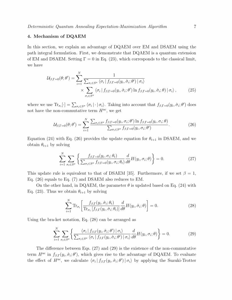
4. Mechanism of DQAEM

In this section, we explain an advantage of DQAEM over EM and DSAEM using the

path integral formulation. First, we demonstrate that DQAEM is a quantum extension

of EM and DSAEM. Setting Γ = 0 in Eq. (23), which corresponds to the classical limit,

we have

Uβ,Γ=0(θ; θ′) =N∑i=1

1∑σi∈Sσ 〈σi | fβ,Γ=0(yi, σi; θ′) |σi〉

×∑σi∈Sσ

〈σi | fβ,Γ=0(yi, σi; θ′) ln fβ,Γ=0(yi, σi; θ) |σi〉 , (25)

where we use Trσi [·] =∑

σi∈Sσ 〈σi | · |σi〉. Taking into account that fβ,Γ=0(yi, σi; θ′) does

not have the non-commutative term Hnc, we get

Uβ,Γ=0(θ; θ′) =N∑i=1

∑σi∈Sσ fβ,Γ=0(yi, σi; θ

′) ln fβ,Γ=0(yi, σi; θ)∑σi∈Sσ fβ,Γ=0(yi, σi; θ′)

. (26)

Equation (24) with Eq. (26) provides the update equation for θt+1 in DSAEM, and we

obtain θt+1 by solving

N∑i=1

∑σi∈Sσ

{fβ,Γ=0(yi, σi; θt)∑

σi∈Sσ fβ,Γ=0(yi, σi; θt)

d

dθH(yi, σi; θ)

}= 0. (27)

This update rule is equivalent to that of DSAEM [35]. Furthermore, if we set β = 1,

Eq. (26) equals to Eq. (7) and DSAEM also reduces to EM.

On the other hand, in DQAEM, the parameter θ is updated based on Eq. (24) with

Eq. (23). Thus we obtain θt+1 by solving

N∑i=1

Trσi

[fβ,Γ(yi, σi; θt)

Trσi [fβ,Γ(yi, σi; θt)]

d

dθH(yi, σi; θ)

]= 0. (28)

Using the bra-ket notation, Eq. (28) can be arranged as

N∑i=1

∑σi∈Sσ

{ 〈σi | fβ,Γ(yi, σi; θ′) |σi〉∑

σi∈Sσ 〈σi | fβ,Γ(yi, σi; θ′) |σi〉d

dθH(yi, σi; θ)

}= 0. (29)

The difference between Eqs. (27) and (29) is the existence of the non-commutative

term Hnc in fβ,Γ(yi, σi; θ′), which gives rise to the advantage of DQAEM. To evaluate

the effect of Hnc, we calculate 〈σi | fβ,Γ(yi, σi; θ′) |σi〉 by applying the Suzuki-Trotter

Deterministic Quantum Annealing Expectation-Maximization Algorithm 8

expansion [33]. Then we obtain

〈σi | fβ,Γ(yi, σi; θ′) |σi〉

= limM→∞

∑σ′i,1,σi,1,...,σi,M−1,σ

′i,M∈Sσ

M∏j=1

⟨σi,j

∣∣∣ e− βMH(yi,σi;θ

′)∣∣∣σ′i,j⟩⟨σ′i,j ∣∣∣ e− β

MHnc∣∣∣σi,j−1

⟩,

(30)

= limM→∞

∑σi,1,σi,2,...,σi,M−1∈Sσ

M∏j=1

⟨σi,j

∣∣∣ e− βMH(yi,σi;θ

′)∣∣∣σi,j⟩⟨σi,j ∣∣∣ e− β

MHnc∣∣∣σi,j−1

⟩, (31)

with the boundary conditions |σi,0〉 = |σi,M〉 = |σi〉 and 〈σi,0| = 〈σi,M | = 〈σi|. In

Eq. (31), the quantum effect comes from⟨σi,j

∣∣∣ e− βMHnc∣∣∣σi,j−1

⟩. If we assume the

classical case Hnc = 0 (i.e. Γ = 0), we obtain⟨σi,j

∣∣∣ e− βMHnc∣∣∣σi,j−1

⟩= 〈σi,j |σi,j−1〉 =

δσi,j ,σi,j−1, where δ·,· is the Kronecker delta function. Thus, |σi,j〉 does not depend on

the index along the Trotter dimension, j. In terms of the path integral formulation,

this fact implies that 〈σi | fβ,Γ(yi, σi; θ′) |σi〉 can be evaluated by a single classical path

with the boundary condition fixed at σi; see Fig. 1. On the other hand, in the quantum

case,⟨σi,j

∣∣∣ e− βMHnc∣∣∣σi,j−1

⟩6= 〈σi,j |σi,j−1〉, and therefore Eq. (31) involves not only the

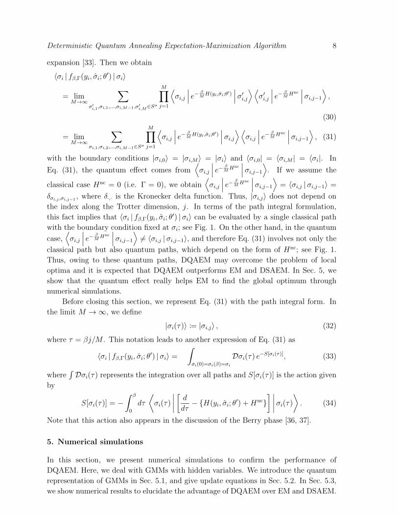
classical path but also quantum paths, which depend on the form of Hnc; see Fig. 1.

Thus, owing to these quantum paths, DQAEM may overcome the problem of local

optima and it is expected that DQAEM outperforms EM and DSAEM. In Sec. 5, we

show that the quantum effect really helps EM to find the global optimum through

numerical simulations.

Before closing this section, we represent Eq. (31) with the path integral form. In

the limit M →∞, we define

|σi(τ)〉 := |σi,j〉 , (32)

where τ = βj/M . This notation leads to another expression of Eq. (31) as

〈σi | fβ,Γ(yi, σi; θ′) |σi〉 =

∫σi(0)=σi(β)=σi

Dσi(τ) e−S[σi(τ)], (33)

where∫Dσi(τ) represents the integration over all paths and S[σi(τ)] is the action given

by

S[σi(τ)] = −∫ β

0

dτ

⟨σi(τ)

∣∣∣∣ [ ddτ − {H(yi, σi; θ′) +Hnc}

] ∣∣∣∣σi(τ)

⟩. (34)

Note that this action also appears in the discussion of the Berry phase [36, 37].

5. Numerical simulations

In this section, we present numerical simulations to confirm the performance of

DQAEM. Here, we deal with GMMs with hidden variables. We introduce the quantum

representation of GMMs in Sec. 5.1, and give update equations in Sec. 5.2. In Sec. 5.3,

we show numerical results to elucidate the advantage of DQAEM over EM and DSAEM.

Deterministic Quantum Annealing Expectation-Maximization Algorithm 9

σi

j0 1 2 3 . . . . . . M

Classical path

Quantum path

Figure 1: Schematic of classical paths (solid line) and quantum paths (dashed line) with the

boundary condition σi = σi,0 = σi,M . The axis represents the Trotter dimension

j (0 ≤ j ≤M). Quantum paths have jumps from state to state while classical paths do not.

In EM and DSAEM, only classical path (solid line) contribute to Eq. (31). In contrast, in

DQAEM, we need to sum over all quantum paths (dashed line).

5.1. Gaussian mixture models

First, we provide a concrete setup of GMMs. Consider that a GMM is composed of K

Gaussian functions and the domain of the hidden variables Sσ is given by {1, 2, . . . , K} §.Then the distribution of the GMM is written by

f(yi, σi; θ) =K∑k=1

πkg(yi;µk,Σk)δσi,k, (35)

where gk(yi;µk,Σk) is the k-th Gaussian function of the GMM parametrized by {µk,Σk},

and δ·,· is the Kronecker delta. The parameters {πk}Kk=1 stand for the mixing ratios

that satisfy∑K

k=1 πk = 1. Here, we denote all the parameters collectively by θ:

θ = {πk, µk,Σk}Kk=1. From Eq. (15), we get the Hamiltonian of this system:

H(yi, σi; θ) =K∑k=1

hki δσi,k, (36)

where we take the logarithm of Eq. (35) and hki = − ln(πkg(yi;µk,Σk)).

Next, following the discussion of Sec. 3, we define the ket vector |σi〉, and the

operator σi as

σi |σi = k〉 = k |σi = k〉 , (37)

where k represents the label of components of the GMM; that is, k ∈ Sσ. To quantize

Eq. (36), we replace σi by σi. Then, we obtain the quantum Hamiltonian of the GMM

§ When we work on the one-hot notation [1, 2], we can formulate an equivalent quantization scheme. [38]

Deterministic Quantum Annealing Expectation-Maximization Algorithm 10

as

H(yi, σi; θ) =K∑k=1

hki δσi,k (38)

=K∑k=1

hki |σi = k〉 〈σi = k| , (39)

where we use δσi,k = |σi = k〉 〈σi = k|. If we adopt the representation,

|σi = k〉 = [0, . . . , 0︸ ︷︷ ︸k−1

, 1, 0, . . . , 0︸ ︷︷ ︸K−k

]ᵀ, (40)

Eq. (39) can be expressed as

H(yi, σi; θ) = diag(h1i , h

2i , . . . , h

Ki ). (41)

Finally we add a non-commutative term Hnc = Γσnc with [σi, σnc] 6= 0 to Eq. (38).

Obviously, there are many candidates for σnc; however, in the numerical simulation, we

adopt

σnc =∑

k=1,...,Kl=k±1

|σi = l〉 〈σi = k| , (42)

where |σi = 0〉 = |σi = K〉 and |σi = K + 1〉 = |σi = 1〉. This term induces quantum

paths shown in Fig. 1.

5.2. Update equations

Suppose that we have N data points Yobs = {y1, y2, . . . , yN}, and they are independent

and identically distributed obeying a GMM. In EM, the update equations of GMMs

are obtained by Eq. (8) with the constraint∑K

k=1 πk = 1; then the parameters at the

(t+ 1)-th iteration, θt+1, are given by

πkt+1 =Nk

N, (43)

µkt+1 =1

Nk

N∑i=1

yif(yi, σi = k; θt)∑σi∈Sσ f(yi, σi; θt)

, (44)

Σkt+1 =

1

Nk

N∑i=1

(yi − µkt+1)(yi − µkt+1)ᵀf(yi, σi = k; θt)∑σi∈Sσ f(yi, σi; θt)

, (45)

where Nk =∑N

i=1f(yi,σi=k;θt)∑σi∈Sσ

f(yi,σi;θt), θt is the tentative estimated parameter at the t-th

iteration.

Deterministic Quantum Annealing Expectation-Maximization Algorithm 11

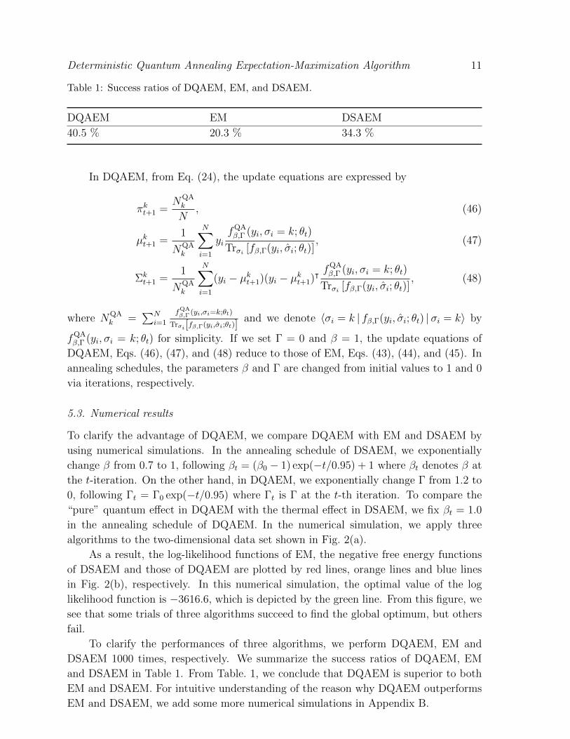
Table 1: Success ratios of DQAEM, EM, and DSAEM.

DQAEM EM DSAEM

40.5 % 20.3 % 34.3 %

In DQAEM, from Eq. (24), the update equations are expressed by

πkt+1 =NQAk

N, (46)

µkt+1 =1

NQAk

N∑i=1

yifQAβ,Γ (yi, σi = k; θt)

Trσi [fβ,Γ(yi, σi; θt)], (47)

Σkt+1 =

1

NQAk

N∑i=1

(yi − µkt+1)(yi − µkt+1)ᵀfQAβ,Γ (yi, σi = k; θt)

Trσi [fβ,Γ(yi, σi; θt)], (48)

where NQAk =

∑Ni=1

fQAβ,Γ (yi,σi=k;θt)

Trσi [fβ,Γ(yi,σi;θt)]and we denote 〈σi = k | fβ,Γ(yi, σi; θt) |σi = k〉 by

fQAβ,Γ (yi, σi = k; θt) for simplicity. If we set Γ = 0 and β = 1, the update equations of

DQAEM, Eqs. (46), (47), and (48) reduce to those of EM, Eqs. (43), (44), and (45). In

annealing schedules, the parameters β and Γ are changed from initial values to 1 and 0

via iterations, respectively.

5.3. Numerical results

To clarify the advantage of DQAEM, we compare DQAEM with EM and DSAEM by

using numerical simulations. In the annealing schedule of DSAEM, we exponentially

change β from 0.7 to 1, following βt = (β0 − 1) exp(−t/0.95) + 1 where βt denotes β at

the t-iteration. On the other hand, in DQAEM, we exponentially change Γ from 1.2 to

0, following Γt = Γ0 exp(−t/0.95) where Γt is Γ at the t-th iteration. To compare the

“pure” quantum effect in DQAEM with the thermal effect in DSAEM, we fix βt = 1.0

in the annealing schedule of DQAEM. In the numerical simulation, we apply three

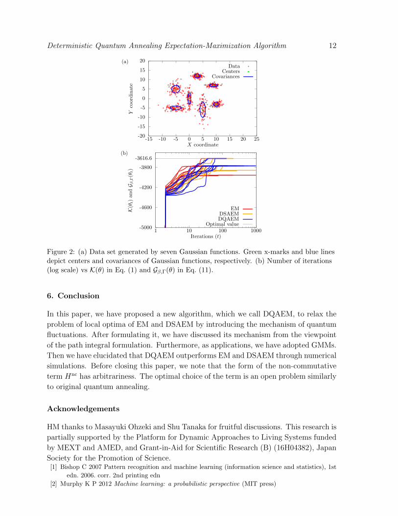
algorithms to the two-dimensional data set shown in Fig. 2(a).

As a result, the log-likelihood functions of EM, the negative free energy functions

of DSAEM and those of DQAEM are plotted by red lines, orange lines and blue lines

in Fig. 2(b), respectively. In this numerical simulation, the optimal value of the log

likelihood function is −3616.6, which is depicted by the green line. From this figure, we

see that some trials of three algorithms succeed to find the global optimum, but others

fail.

To clarify the performances of three algorithms, we perform DQAEM, EM and

DSAEM 1000 times, respectively. We summarize the success ratios of DQAEM, EM

and DSAEM in Table 1. From Table. 1, we conclude that DQAEM is superior to both

EM and DSAEM. For intuitive understanding of the reason why DQAEM outperforms

EM and DSAEM, we add some more numerical simulations in Appendix B.

Deterministic Quantum Annealing Expectation-Maximization Algorithm 12

(a)

-20

-15

-10

-5

0

5

10

15

20

-15 -10 -5 0 5 10 15 20 25

Yco

ord

inat

e

X coordinate

DataCenters

Covariances

(b)

-5000

-4600

-4200

-3800

-3616.6

1 10 100 1000

K(θ

t)

and

G β,Γ

(θt)

Iterations (t)

EMDSAEMDQAEM

Optimal value

Figure 2: (a) Data set generated by seven Gaussian functions. Green x-marks and blue lines

depict centers and covariances of Gaussian functions, respectively. (b) Number of iterations

(log scale) vs K(θ) in Eq. (1) and Gβ,Γ(θ) in Eq. (11).

6. Conclusion

In this paper, we have proposed a new algorithm, which we call DQAEM, to relax the

problem of local optima of EM and DSAEM by introducing the mechanism of quantum

fluctuations. After formulating it, we have discussed its mechanism from the viewpoint

of the path integral formulation. Furthermore, as applications, we have adopted GMMs.

Then we have elucidated that DQAEM outperforms EM and DSAEM through numerical

simulations. Before closing this paper, we note that the form of the non-commutative

term Hnc has arbitrariness. The optimal choice of the term is an open problem similarly

to original quantum annealing.

Acknowledgements

HM thanks to Masayuki Ohzeki and Shu Tanaka for fruitful discussions. This research is

partially supported by the Platform for Dynamic Approaches to Living Systems funded

by MEXT and AMED, and Grant-in-Aid for Scientific Research (B) (16H04382), Japan

Society for the Promotion of Science.[1] Bishop C 2007 Pattern recognition and machine learning (information science and statistics), 1st

edn. 2006. corr. 2nd printing edn

[2] Murphy K P 2012 Machine learning: a probabilistic perspective (MIT press)

Deterministic Quantum Annealing Expectation-Maximization Algorithm 13

[3] Dempster A P, Laird N M and Rubin D B 1977 Journal of the Royal Statistical Society, Series B

39 1–38

[4] Kirkpatrick S, Gelatt C D and Vecchi M P 1983 Science 220 671–680 URL http://www.

sciencemag.org/content/220/4598/671.abstract

[5] Kirkpatrick S 1984 Journal of Statistical Physics 34 975–986 ISSN 0022-4715 URL http:

//dx.doi.org/10.1007/BF01009452

[6] Geman S and Geman D 1984 Pattern Analysis and Machine Intelligence, IEEE Transactions on

PAMI-6 721–741 ISSN 0162-8828

[7] Rose K, Gurewitz E and Fox G 1990 Pattern Recognition Letters 11 589–594 ISSN 0167-8655 URL

http://www.sciencedirect.com/science/article/pii/016786559090010Y

[8] Rose K, Gurewitz E and Fox G C 1990 Phys. Rev. Lett. 65(8) 945–948 URL http://link.aps.

org/doi/10.1103/PhysRevLett.65.945

[9] Ueda N and Nakano R 1998 Neural Networks 11 271–282 ISSN 0893-6080 URL http://www.

sciencedirect.com/science/article/pii/S0893608097001330

[10] Apolloni B, Carvalho C and de Falco D 1989 Stochastic Processes and their Applications

33 233–244 ISSN 0304-4149 URL http://www.sciencedirect.com/science/article/pii/

0304414989900409

[11] Finnila A, Gomez M, Sebenik C, Stenson C and Doll J 1994 Chemical Physics Letters

219 343–348 ISSN 0009-2614 URL http://www.sciencedirect.com/science/article/pii/

0009261494001170

[12] Kadowaki T and Nishimori H 1998 Phys. Rev. E 58(5) 5355–5363 URL http://link.aps.org/

doi/10.1103/PhysRevE.58.5355

[13] Santoro G E, Martonak R, Tosatti E and Car R 2002 Science 295 2427–2430 URL http:

//www.sciencemag.org/content/295/5564/2427.abstract

[14] Santoro G E and Tosatti E 2006 Journal of Physics A: Mathematical and General 39 R393

[15] Farhi E, Goldstone J, Gutmann S, Lapan J, Lundgren A and Preda D 2001 Science 292 472–475

URL http://www.sciencemag.org/content/292/5516/472.abstract

[16] Morita S and Nishimori H 2008 Journal of Mathematical Physics 49 125210 URL http://

scitation.aip.org/content/aip/journal/jmp/49/12/10.1063/1.2995837

[17] Brooke J, Bitko D, F T, Rosenbaum and Aeppli G 1999 Science 284 779–781 URL http:

//www.sciencemag.org/content/284/5415/779.abstract

[18] de Falco D and Tamascelli D 2009 Phys. Rev. A 79(1) 012315 URL http://link.aps.org/doi/

10.1103/PhysRevA.79.012315

[19] de Falco D and Tamascelli D 2011 RAIRO - Theoretical Informatics and Applications 45(01)

99–116 ISSN 1290-385X

[20] Das A and Chakrabarti B K 2008 Rev. Mod. Phys. 80(3) 1061–1081 URL http://link.aps.org/

doi/10.1103/RevModPhys.80.1061

[21] Martonak R, Santoro G E and Tosatti E 2002 Phys. Rev. B 66(9) 094203 URL http://link.

aps.org/doi/10.1103/PhysRevB.66.094203

[22] Lloyd S, Mohseni M and Rebentrost P 2013 arXiv preprint arXiv:1307.0411

[23] Rebentrost P, Mohseni M and Lloyd S 2014 Phys. Rev. Lett. 113(13) 130503 URL http:

//link.aps.org/doi/10.1103/PhysRevLett.113.130503

[24] Nathan Wiebe Ashish Kapoor K M S 2014 Quantum deep learning URL https://www.microsoft.

com/en-us/research/publication/quantum-deep-learning/

[25] Johnson M, Amin M, Gildert S, Lanting T, Hamze F, Dickson N, Harris R, Berkley A, Johansson

J, Bunyk P et al. 2011 Nature 473 194–198

[26] Schuld M, Sinayskiy I and Petruccione F 2015 Contemporary Physics 56 172–185 (Preprint

http://dx.doi.org/10.1080/00107514.2014.964942) URL http://dx.doi.org/10.1080/

00107514.2014.964942

[27] Aaronson S 2015 Nature Physics 11 291–293

[28] Rebentrost P, Mohseni M and Lloyd S 2014 Phys. Rev. Lett. 113(13) 130503 URL http:

Deterministic Quantum Annealing Expectation-Maximization Algorithm 14

//link.aps.org/doi/10.1103/PhysRevLett.113.130503

[29] Xu L and Jordan M I 1996 Neural computation 8 129–151

[30] Kullback S and Leibler R A 1951 The annals of mathematical statistics 22 79–86

[31] Kullback S 1997 Information Theory and Statistics (Dover Publications)

[32] Umegaki H 1962 Kodai Mathematical Seminar Reports 14 59–85

[33] Suzuki M 1976 Progress of Theoretical Physics 56 1454–1469 URL http://ptp.oxfordjournals.

org/content/56/5/1454.abstract

[34] Al-Mohy A H and Higham N J 2010 SIAM Journal on Matrix Analysis and Applications 31 970–

989 (Preprint http://dx.doi.org/10.1137/09074721X) URL http://dx.doi.org/10.1137/

09074721X

[35] Ueda N and Nakano R 1998 Neural Networks 11 271–282 ISSN 0893–6080 URL http://www.

sciencedirect.com/science/article/pii/S0893608097001330

[36] Berry M V 1985 Journal of Physics A: Mathematical and General 18 15 URL http://stacks.

iop.org/0305-4470/18/i=1/a=012

[37] Nagaosa N 2013 Quantum field theory in condensed matter physics (Springer Science & Business

Media)

[38] Miyahara H, Tsumura K and Sughiyama Y 2016 Relaxation of the em algorithm via quantum

annealing for gaussian mixture models 2016 IEEE 55th Conference on Decision and Control

(CDC) pp 4674–4679

[39] Wu C F J 1983 Ann. Statist. 11 95–103 URL http://dx.doi.org/10.1214/aos/1176346060

Appendix A. Convergence theorem

We give a theorem that the negative free energy function has monotonicity for iterations.

Theorem 1. Let θt+1 = arg maxθ Uβ,Γ(θ; θt). Then Gβ,Γ(θt+1) ≥ Gβ,Γ(θt) holds.

Proof. First, the difference of the free energy functions in each iteration can be written

as

∆Gβ,Γ = Gβ,Γ(θt+1)− Gβ,Γ(θt) (A.1)

=1

β(Uβ,Γ(θt+1; θt)− Uβ,Γ(θt; θt))−

1

β(Sβ,Γ(θt+1; θt)− Sβ,Γ(θt; θt)), (A.2)

where

Sβ,Γ(θ; θ′) =N∑i=1

Trσi

[fβ,Γ(yi, σi; θ

′)

Trσi [fβ,Γ(yi, σi; θ′)]ln

fβ,Γ(yi, σi; θ)

Trσi [fβ,Γ(yi, σi; θ)]

]. (A.3)

The first two terms in the right hand side of Eq. (A.2) is positive due to Eq. (24).

Furthermore, we can show that the rest of the right hand side of Eq. (A.2) are positive

by the following calculations:

−(Sβ,Γ(θt+1; θt)− Sβ,Γ(θt; θt))

= KL

(fβ,Γ(yi, σi; θt+1)

Trσi [fβ,Γ(yi, σi; θt+1)]

∥∥∥∥ fβ,Γ(yi, σi; θt)

Trσi [fβ,Γ(yi, σi; θt)]

)≥ 0. (A.4)

Deterministic Quantum Annealing Expectation-Maximization Algorithm 15

This theorem insists that DQAEM converges to at least the global optimum or a

local optimum. The global convergence of EM is discussed by Dempster et al. [3] and

Wu [39], and their discussion is available to DQAEM.

Appendix B. Numerical results

We discuss the performances of DQAEM, EM, and DSAEM by showing how the

landscape of the negative free energy function behaves when β and Γ are changed.

For simplicity, we assume that a GMM is composed of two one-dimensional Gaussian

functions and consider the case where only means of two Gaussian functions are

estimated. Accordingly, the joint probability density function is given by

f(yi, σi; θ = {µ1, µ2}) =2∏

k=1

πkg(yi;µk,Σk)δσi,k, (B.1)

where g(yi;µ,Σ) is a Gaussian function with mean µ and covariance Σ. Under this setup,

we estimate θ = {µ1, µ2}: we assume that θ = {µ1, µ2} are unknown and {π1, π2,Σ1,Σ2}are given.

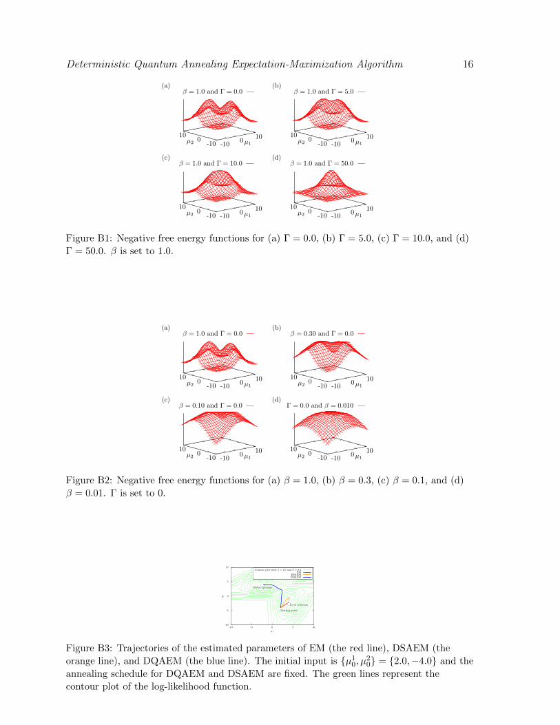
First, let us describe the landscapes of the negative free energy functions with

different β and Γ. We plot the negative free energy functions of DQAEM at Γ = 0.0,

5.0, 10.0, and 50.0 with β = 1 in Fig. B1(a), (b), (c), and (d), respectively. Specifically,

Fig. B1(a) describes the log-likelihood function, since DQAEM reduces to EM at β = 1

and Γ = 0. In our example used here, the global optimal value for {µ1, µ2} is {−2.0, 4.0}(the left top in Fig. B1(a)) and the point {4.0,−2.0} (the right top in Fig. B1(a)) is

the local optimum. If we set the initial value at a point close to the local optimum,

EM fails to find the global optimum. In contrast, Fig. B1 shows that the negative free

energy function changes from a multimodal form to a unimodal form when Γ increases.

Thus, even if we set the initial value close to the local optimum, DQAEM may find the

global optimum through the annealing process. On the other hand, in Fig. B2, we plot

the negative free energy functions of DSAEM at inverse temperature β = 1.0, 0.3, 0.1,

and 0.01. DSAEM has the similar effect in the negative free energy function.

However, as we have seen in Sec. 5.3, they differ qualitatively. To understand this

fact intuitively, we show the trajectories of the estimated parameters of EM, DSAEM,

and DQAEM in Fig. B3. In this numerical simulation, the initial parameter θ0 is set

near the local optimum in the log-likelihood function. The red line depicts the trajectory

of the estimated parameter of EM and goes to the local optimum orthogonally crossing

the contour plots. As shown by the orange line, DSAEM eventually fails to find the

global optimum as same as the case of EM. On the other hand, the estimated parameter

θt of DQAEM shown by the blue line surmounts the potential barrier and reaches the

global optimum. Accordingly, we consider that DQAEM outperforms EM and DSAEM.

Deterministic Quantum Annealing Expectation-Maximization Algorithm 16

(a)

-100

10-10

010

β = 1.0 and Γ = 0.0

µ1µ2

(b)

-100

10-10

010

β = 1.0 and Γ = 5.0

µ1µ2

(c)

-100

10-10

010

β = 1.0 and Γ = 10.0

µ1µ2

(d)

-100

10-10

010

β = 1.0 and Γ = 50.0

µ1µ2

Figure B1: Negative free energy functions for (a) Γ = 0.0, (b) Γ = 5.0, (c) Γ = 10.0, and (d)

Γ = 50.0. β is set to 1.0.

(a)

-100

10-10

010

β = 1.0 and Γ = 0.0

µ1µ2

(b)

-100

10-10

010

β = 0.30 and Γ = 0.0

µ1µ2

(c)

-100

10-10

010

β = 0.10 and Γ = 0.0

µ1µ2

(d)

-100

10-10

010

Γ = 0.0 and β = 0.010

µ1µ2

Figure B2: Negative free energy functions for (a) β = 1.0, (b) β = 0.3, (c) β = 0.1, and (d)

β = 0.01. Γ is set to 0.

-10

-5

0

5

10

-10 -5 0 5 10

µ2

µ1

Starting point

Local optimum

Global optimum

Contour plot with β = 1.0 and Γ = 0.0EM

DSAEMDQAEM

Figure B3: Trajectories of the estimated parameters of EM (the red line), DSAEM (the

orange line), and DQAEM (the blue line). The initial input is {µ10, µ

20} = {2.0,−4.0} and the

annealing schedule for DQAEM and DSAEM are fixed. The green lines represent the

contour plot of the log-likelihood function.