Determining Well Control Issues in HTHP Wells by ...
93
i Determining Well Control Issues in HTHP Wells by Predicting Equivalent Circulating Density By Mohammad Adi Aiman Haji Sarbini G01539 Dissertation submitted in partial fulfilment of the requirements for the MSc Petroleum Engineering (MSc PE) JULY 2012 Universiti Teknologi PETRONAS 32610 Bandar Seri Iskandar Perak Darul Ridzuan
Transcript of Determining Well Control Issues in HTHP Wells by ...
i
Determining Well Control Issues in HTHP Wells by
Predicting Equivalent Circulating Density
By
Mohammad Adi Aiman Haji Sarbini
G01539
Dissertation submitted in partial fulfilment of
the requirements for the
MSc Petroleum Engineering
(MSc PE)
JULY 2012
Universiti Teknologi PETRONAS
32610 Bandar Seri Iskandar
Perak Darul Ridzuan
ii
CERTIFICATION OF APPROVAL
Determining Well Control Issues in HTHP Wells by
Predicting Equivalent Circulating Density
By
Mohammad Adi Aiman Haji Sarbini
G01539
A project dissertation submitted to the
Petroleum Engineering Programme
Universiti Teknologi PETRONAS
in partial fulfilment of the requirement for the
MSc of PETROLEUM ENGINEERING
Approved by,
_______________________
(Dr. Ismail M Saaid)
UNIVERSITI TEKNOLOGI PETRONAS
TRONOH, PERAK
JULY 2012

iii
CERTIFICATION OF ORIGINALITY
This is to certify that I am responsible for the work submitted in this project, that the
original work is my own except as specified in the references and
acknowledgements, and that the original work contained herein have not been
undertaken or done by unspecified sources or persons.
______________________________
Mohammad Adi Aiman Haji Sarbini

iv
ACKNOWLEDGEMENTS
First of all I would like to express our gratitude to all those who has contributed in
any way for the success of this Individual Project. I would like to take this
opportunity to thank my direct supervisor of this project; Dr. Sonny Irawan. I am
also deeply indebted to Pg. Amirrudin Pg. Hj. Razali (PetroleumBRUNEI), Hairol
Nizam Mokti (PetroleumBRUNEI) for their guidance and useful suggestions which
helped us in completing this project in time.
Finally, yet importantly, I would like to express our heartfelt thanks to our beloved
family for their blessings, our friends and classmates for their help and wishes for the
successful completion of this project.
v
ABSTRACT
Well control issues are caused mainly due to pressure instabilities in the wellbore.
For example, when the hydrostatic pressure exerted by the mud column is being
overcome by the pore pressure, the formation fluids start to invade the wellbore. This
well control problem is also known as “kick”. Well control issues can also be caused
when there is too much hydrostatic pressure exerted by the mud column which
causes the formation to fracture. This formation fractures can mitigate, thus create a
flow conduit in the formation where the drilling fluid can permeate and be lost – a
common well control problem known as “lost circulation”. Furthermore, high
temperature and high pressure formation normally has the issue of narrow
bottomhole pressure margin between the pore pressure and the fracture pressure.
This characteristic of the HTHP well means that there is a little margin for error
when choosing the right mud weight and the mud components that can function
properly within this margin. The problem is further complicated during circulation as
the mud weight is increased depending on the amount of frictional pressure loss
along the flow conduits, now defined as equivalent circulating density (ECD).
Predicting the ECD requires circulating fluid temperatures to be simulated, which is
built using implicit numerical methods by applying Crank-Nicolson solution. This
temperature simulator is used in conjunction with the temperature and pressure
dependent rheological properties of drilling fluids to evaluate the ECD. The results
show that the bottomhole fluid temperature decreases with increasing circulation
time and circulation rate, which consequently increase the ECD, which may lead to
formation fracture. Furthermore, geothermal gradient is found to be the most
sensitive parameter that may lead to well control problems if a linear gradient is
assumed especially in heterogeneous HTHP formations. Therefore, choosing the
right drilling fluid constituents that are stable in high temperature and high pressure,
and compatible to be used in HTHP formation is critical to ensure well control issues
are minimized.

vi
SUMMARY
This project commenced officially on the 25th
March 2012 and ended on the 22nd
June 2012. During the first two weeks, literature reviews were being done from SPE
journals as well as course notes, which consequently allowed me to develop clear
objectives for this project. The following weeks were dedicated to develop the
methodology, collecting data, developing mathematical models as well as simulating
model to obtain results.
Building the model for temperature require the understanding of heat flow equations
between the formation and inside the wellbore. Separate fluid temperature must also
be taken into account for the fluid flowing down the drillpipe as well as up the
annulus. The knowledge of fluid temperature profiles in both flow conduits allows
the evaluation of ECD at the openhole. This requires a compositional model in order
to predict the downhole density as a function of temperature and pressure. The
evaluation of ECD also requires calculations of frictional pressure losses during fluid
flow to be made. Two flow regimes could be considered to calculate this pressure
loss i.e. laminar and turbulent flow. However, due to time constraints, an only
pressure loss due to laminar flow was studied.
The prediction results show that during circulation, the fluid temperature at the
openhole decreases with circulation time and circulation rate. This temperature
reduction causes the density at that openhole to increase, thus, creating a fracture risk
in HTHP formations, which have narrow pore and fracture pressure margins.
The biggest challenge in this project is to build a prediction model. This is where the
majority of time was spent building such simulation model as it involved learning to
program on Macro in Microsoft Excel that was able to numerically solve heat flow
equations implicitly, and thus, predict circulating fluid temperature inside the
wellbore.
vii
Table of Contents
............................................................................. 1 CHAPTER 1: INTRODUCTION
1.1 Problem Statements ................................................................................... 1
1.2 Objectives .................................................................................................... 1
1.3 Scope of Study ............................................................................................ 2
1.4 Data Availability ........................................................................................ 2
1.5 Project Schedule & Organization ............................................................. 2
................................................................. 3 CHAPTER 2: LITERATURE REVIEW
2.1 Geothermal Gradients ............................................................................... 3
2.2 High Temperature High Pressure ............................................................ 3
2.2.1 Classifications .......................................................................................... 4
2.2.2 Characteristics of HTHP Wells ................................................................ 5
2.3 Properties of Drilling Fluids ...................................................................... 5
2.3.1 Functions .................................................................................................. 5
2.3.2 Composition ............................................................................................. 6
2.3.3 Physical Properties ................................................................................... 6
2.3.4 Density ..................................................................................................... 7
2.3.5 Flow Regimes .......................................................................................... 7
2.3.6 Rheology Models ..................................................................................... 9
2.4 Equivalent Circulating Density ............................................................... 11
2.4.1 Equivalent Static Density ....................................................................... 11
2.4.2 Frictional Pressure Loss ......................................................................... 12
2.4.3 Equivalent Circulating Density .............................................................. 12
2.5 Review of Finite Difference Scheme ....................................................... 12
2.5.1 Explicit Solution .................................................................................... 15
2.5.2 Implicit Solution .................................................................................... 16
.......................................................................... 19 CHAPTER 3: METHODOLOGY
3.1 Overall ....................................................................................................... 19
3.2 Drilling Fluids in HTHP Conditions ...................................................... 19
3.3 Temperature Estimation ......................................................................... 20
3.3.1 Analytical Approach .............................................................................. 21
3.3.2 Numerical Solutions ............................................................................... 21
viii
3.4 ECD Model ............................................................................................... 21
.......................... 22 CHAPTER 4: DRILLING FLUIDS IN HTHP CONDITIONS
4.1 Influence on Mud Temperature .............................................................. 22
4.2 Influence on Mud Density ....................................................................... 22
4.3 Influence on Rheology ............................................................................. 23
4.3.1 Physical properties ................................................................................. 24
4.3.2 Chemical properties ............................................................................... 24
4.3.3 Electrochemical properties ..................................................................... 24
4.4 Critical Temperature ............................................................................... 24
4.5 Rheology Experiments ............................................................................. 25
4.5.1 Time-independent properties ................................................................. 26
4.5.2 Time-dependent properties..................................................................... 26
4.6 Limitations ................................................................................................ 26
................................. 28 CHAPTER 5: TEMPERATURE PREDICTION MODEL
5.1 Geothermal Gradient ............................................................................... 28
5.2 Drilling Fluid Temperature ..................................................................... 29
5.3 Heat Transfer (Analytical) ...................................................................... 29
5.3.1 First Stage: Drillpipe .............................................................................. 30
5.3.2 Second Stage: Bottomhole ..................................................................... 31
5.3.3 Third Stage: Annulus ............................................................................. 32
5.4 Heat Transfer (Numerical) ...................................................................... 34
5.4.1 Conservation of Energy in the Wellbore and Formation ....................... 35
5.4.2 Discretization of Heat Flow Equations .................................................. 37
5.5 Explicit Method ........................................................................................ 37
5.6 Implicit Method ........................................................................................ 41
5.7 Boundary Conditions ............................................................................... 44
5.7.1 Drillpipe Boundary Conditions .............................................................. 45
5.7.2 Annulus Boundary Conditions ............................................................... 45
5.7.3 Formation Boundary Conditions ............................................................ 46
........................................................ 48 CHAPTER 6: ECD PREDICTION MODEL
6.1 Static Mud Density ................................................................................... 48
6.2 Compositional Model ............................................................................... 48
6.3 Rheological Model .................................................................................... 50
ix
6.3.1 Plastic Viscosity ..................................................................................... 50
6.3.2 Yield Point ............................................................................................. 51
6.4 ECD Model ............................................................................................... 51
6.4.1 Volumetric Behaviour of Oil Phase ....................................................... 52
6.4.2 Volumetric Behaviour of Water Phase .................................................. 53
6.4.3 Evaluating Frictional Pressure Loss ....................................................... 53
6.5 Evaluating ECD ........................................................................................ 55
......................................................... 56 CHAPTER 7: RESULTS & DISCUSSIONS
7.1 Static Density Model ................................................................................ 56
7.2 ECD Prediction Model ............................................................................. 57
7.2.1 Results .................................................................................................... 57
7.3 Parameter Study....................................................................................... 61
7.3.1 Circulation Time .................................................................................... 61
7.3.2 Circulation Rates .................................................................................... 62
7.3.3 Geothermal Gradients ............................................................................ 65
7.4 Sensitivity Analysis .................................................................................. 66
7.5 Discussions on Prediction Models ........................................................... 68
7.5.1 Temperature Model ................................................................................ 68
7.5.2 ECD Model ............................................................................................ 69
7.6 Determining Well Control Issues from ECD ......................................... 70
.............................................................................. 71 CHAPTER 8: CONCLUSIONS
8.1 Practical Applications .............................................................................. 71
8.2 Recommendations .................................................................................... 72
8.2.1 High-Temperature Drilling Fluids ......................................................... 72
8.2.2 Temperature Model ................................................................................ 72
8.2.3 ECD Prediction Model ........................................................................... 73
8.2.4 Sensitivity Analysis ................................................................................ 73
................................................................................ 74 CHAPTER 9: REFERENCES
............................................................................... 77 CHAPTER 10: APPENDICES
10.1 Introduction .............................................................................................. 77
10.2 ECD Model Prediction ............................................................................. 77
x
Table of Figures
Figure 2.1: Classification of HTHP formations ........................................................... 5
Figure 2.2: Illustration of laminar flow inside a drillpipe ............................................ 8
Figure 2.3: Illustration of turbulent flow inside a drillpipe .......................................... 8
Figure 2.4: Relationship between laminar flow and turbulent flow ............................. 9
Figure 2.5: Model of Viscous Forces in Fluids .......................................................... 10
Figure 2.6: Comparison between different rheological models ................................. 11
Figure 2.7: Graphical representation of the finite difference derivatives calculated
using forward difference, backward difference and central difference. (Reservoir
Simulation, Heriot-Watt University) .......................................................................... 13
Figure 2.8: Schematic of explicit finite difference algorithm for solving simple
partial differential equation (Reservoir Simulation, Heriot-Watt University) ........... 16
Figure 2.9: A 5 grid block system showing how implicit finite difference scheme
works. (Reservoir Simulation, Heriot-Watt University) ............................................ 18
Figure 2.10: Schematic of explicit finite difference algorithm for solving simple
partial differential equation (Reservoir Simulation, Heriot-Watt University) ........... 18
Figure 4.1: Temperature trace for various depths in a simulated well (Courtesy of
Raymond (1969)) ....................................................................................................... 22
Figure 4.2: Effect of temperature and pressure on the density of oil-based and water-
based drilling fluids (McMordie (1982)) ................................................................... 23
Figure 5.1: Circulation stages inside the wellbore ..................................................... 29
Figure 5.2: Schematic of heat flow inside the wellbore for circulating fluid ............ 34
Figure 7.1: Temperature profiles during the initial stage ........................................... 58
Figure 7.2: Simulated wellbore temperature profile for Berambang-1 well .............. 59
Figure 7.3: Simulated equivalent circulating density for Berambang-1 well ............ 60
Figure 7.4: The effects of circulation time with temperature profiles ....................... 61
Figure 7.5: The effects of circulation time on the ECD ............................................. 62
Figure 7.6: Effect of reducing circulation rates on the temperature profiles ............. 63
Figure 7.7: Effect of reducing circulation rates on the ECD ...................................... 64
Figure 7.8: Effect of increasing geothermal gradient on the temperature profiles .... 65
Figure 7.9: Effect of increasing geothermal gradient on the ECD ............................. 66
Figure 7.10: Sensitivity analysis for bottomhole circulating fluid temperature......... 67
Figure 7.11: Sensitivity analysis for ECD.................................................................. 68

xi
Figure 10.1: Project schedule ..................................................................................... 77
xii
List of Tables
Table 4.1: Critical temperatures for several muds and mud components .................. 25
Table 4.2: Conditions applied during rheology experiments ..................................... 25
Table 7.1: Results of density prediction using Kutasov's empirical formula ............. 56
Table 7.2: Input parameters from Berambang-1 well ................................................ 57
Table 10.1: Coefficients of constants for static fluid density..................................... 77
Table 10.2: Empirical constants for equation calculating base oil viscosity ............. 77
Table 10.3: Empirical constants for equation calculating yield point ........................ 78
Table 10.4: Empirical constants for equation calculating the volumetric behaviour of
oil phase ..................................................................................................................... 78
Table 10.5: Empirical constants for equation calculating the volumetric behaviour of
water phase ................................................................................................................. 78
Table 10.6: Bottomhole circulating fluid temperature results from sensitivity analysis
.................................................................................................................................... 78
Table 10.7: Bottomhole equivalent circulating density from sensitivity analysis ..... 78
xiii
Abbreviation
ECD Equivalent Circulating Density
ESD Equivalent Static Density
HTHP High Temperature High Pressure
OBM Oil-Based Mud
SBHP Static Bottom Hole Pressure
UKCSON United Kingdom Continental Shelf Operations Notice
WBM Water-Based Mud
xiv
Nomenclature
surface area of drillpipe (in2)
formation heat transfer coefficient (BTU/lb-
heat capacity of fluid (BTU/lb- )
pipe diameter (in)
inner annular wall (in)
outer annular wall (in)
F force (N)
height of static drilling fluid (ft)
length of flow conduit (ft)
mass flow rate of fluid (gpm),
slope or geothermal gradient (°F/ft)
flow index (dimensionless),
is the pressure loss due to friction
radius of the annulus (in),
radius of the drillpipe (in),
temperature in the formation (°F),
surface temperature (°F)
temperature in the annulus ( ),
temperature in the drillpipe ( ),
temperature of the formation ( ),
heat transfer coefficient between drillpipe and annulus (),
volume of oil components in a drilling fluid
volume of water components in a drilling fluid
volume of solids components in a drilling fluid
volume of chemical components in a drilling fluid
depth (ft)
formation transmissivity (
⁄ )
shear rate
consistency index (N/m2s)
xv
apparent fluid viscosity
mud plastic viscosity at elevated temperature and pressure,
mud plastic viscosity at surface conditions,
base oil plastic viscosity at elevated temperature and pressure,
base oil plastic viscosity at surface conditions.
fluid density (ppg)
formation density (g/cm3),
new density of components subject to HTHP
mud density at reference condition
mud density at elevated temperature and pressure
oil density at reference conditions
oil density at elevated temperature and pressure
water density at reference conditions
water density at elevated temperature and pressure
shear stress,
fluid yield point (N/m2)
yield point at surface conditions (N/m2)
fanning friction factor,
volume fractions of oil and water
volume fractions of oil and water
formation conductivity
fluid velocity (m3/s),
average flow velocity (m3/s),
1
CHAPTER 1
INTRODUCTION
1.1 Problem Statements
High temperature, high pressure (HTHP) formation presents a challenge while
drilling a well. These challenges include how HTHP conditions affect normal drilling
operations and the problems they pose to the stability of the wellbore.
The hydrostatic pressure of the fluid column in a borehole depends on the mud
density and this is different from that on the surface due to the increasing
temperature and pressure with depth. Mud density in the wellbore very well depends
on its rheology, which is also affected by temperature and pressure. While circulating
the drilling fluid, pressure losses are expected, which determine the Equivalent
Circulating Density (ECD). The problem is that mud density and ECD change with
temperature and pressure, and this change alter the behaviour of the drilling fluid,
which consequently affects the wellbore stability and drilling operations, especially
in HTHP wells. Therefore, by predicting ECD, is it possible to predict wellbore
issues?
1.2 Objectives
The main objectives of this project are as follows:
1. To determine the effects of HTHP conditions on the physical and chemical
properties of drilling fluids such as density and rheology
2. To evaluate the impact of these altered properties of drilling fluids (due to
HTHP conditions) on wellbore stability or well control issues
3. To develop a mathematical model to predict:
a. Formation temperature
b. Circulating drilling fluid temperature
c. Equivalent circulating density
2
1.3 Scope of Study
The scope of study in this project involves the geology and the formation of high
temperature, high pressure (HTHP) wells. This subject includes the classifications of
these wells and their distinctive features. The study will also cover drilling
engineering subject, which envelopes related topics to this project such as drilling
fluids, well control and hydraulics. In hydraulics, the flow properties as well as
rheological models will also be studied.
Heat transfer will also be examined in order to understand how heat energy flow
from one medium to another. This will allow the development of a mathematical
model to predict this heat exchange between the formation and the downhole drilling
fluids, which eventually leads to the development of a simulation model to predict
both the bottomhole fluids temperatures as well as the equivalent circulating density.
This will involve the numerical simulation studies using finite difference techniques
and solutions compared between explicit and implicit methods. Several other
methods will also be discussed that would make the numerical simulation more
accurate and efficient such as the Crank-Nicolson and Thomas algorithm.
1.4 Data Availability
Data is made available to be used in this project from an HTHP well in Brunei,
Berambang-1 well. Such data include:
Pore-fracture pressure plot
Temperature gradient
Daily drilling and geological reports
1.5 Project Schedule & Organization
Figure 10.1 in the Appendix shows the project schedule.
3
CHAPTER 2
LITERATURE REVIEW
2.1 Geothermal Gradients
Geothermal gradient is defined as the amount of temperature increase with depth in
the earth’s crust, and is usually expressed in the form of °F/100ft (°C/km). According
to Caenn et al 2011 [1], there are two main sources of heat flow in the upper crust;
1. Heat conduction from the lower crust and mantle
2. Heat produced from radioactive decay in the upper crust
Geothermal gradients vary from place to place depending on a number of factors
such as (Caenn et al 2011 [1]):
The amount of heat produced by radioactive decay in the upper crust
Structural features
Thermal conductivity of the formation; high gradients in low conductivity
zone such as shale and low gradients in high conductivity zones such as
sandstone
Convection flow; for thick permeable formation, water circulates by
convection which creates high temperature at shallow depths
Pore pressure profiles; geopressured formations have higher temperature
gradients
Due to these factors, geothermal gradients have different ranges around the world,
for example, 0.44°F/100ft to 2.7°F/100ft in the United States, and 1.2°F/100ft to
2.2°F.100ft in the Gulf Coast. Steam wells in California have geothermal gradients
as high as 12.5°F/100ft due to water circulating via convection. One finding from
detailed surveys is that geothermal gradients are not linear with depth but depends on
the factors listed above.
2.2 High Temperature High Pressure
United Kingdom Continental Shelf Operations Notice (UKCSON) has defined a
High Temperature, High Pressure (HTHP) as any well that has:
4
A bottomhole temperature starting from 150°C (300°F), or
Pore pressure exceeding 0.8 psi/ft
A bottomhole pressure beyond 10,000 psi
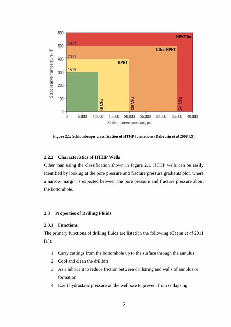
2.2.1 Classifications
Schlumberger (DeBruijn et al 2008 [2]) has classified HTHP formations into three
distinct groups;
1. HTHP
2. Ultra HTHP
3. Extreme HTHP
HTHP wells are identified as those with a minimum bottomhole temperature of
150°C (300°F) or bottomhole pressure of 10,000 psi. For higher bottomhole
temperature of 205°C (400°F) or bottomhole pressure of 20,000 psi, these wells are
called as Ultra HTHP. Finally, Extreme HTHP wells have bottomhole temperatures
beyond 260°C (500°F) or bottomhole pressure of 35,000 psi. Figure 2.1 illustrates
the classification of HTHP wells with their respective pressures and temperatures.
The boundaries between the HTHP classifications represent stability limits of
common tools and components, especially elastomeric seals and electronic
components.
5
Figure 2.1: Schlumberger classification of HTHP formations (DeBruijn et al 2008 [2])
2.2.2 Characteristics of HTHP Wells
Other than using the classification shown in Figure 2.1, HTHP wells can be easily
identified by looking at the pore pressure and fracture pressure gradients plot, where
a narrow margin is expected between the pore pressure and fracture pressure about
the bottomhole.
2.3 Properties of Drilling Fluids
2.3.1 Functions
The primary functions of drilling fluids are listed in the following (Caenn et al 2011
[1]):
1. Carry cuttings from the bottomhole up to the surface through the annulus
2. Cool and clean the drillbits
3. As a lubricant to reduce friction between drillstring and walls of annulus or
formation
4. Exert hydrostatic pressure on the wellbore to prevent from collapsing
6
5. Forms filter cake along the borehole wall to prevent formation fluids from
entering the borehole
2.3.2 Composition
Drilling fluids are identified according to their base fluid, which are; aqueuous, non-
aqueous or gas.
Aqueuous
In water-based (brine) muds, solid particles are suspended which consist of clays,
organic colloids, heavy minerals as well as drill cuttings. These additives provide the
necessary mud properties such as viscosity and filtration properties as well as
density, which aid the abilities of the drilling fluids.
Water-based muds are often composed of bentonite clay, which becomes unstable
with increasing temperatures. This is because at high temperature the adsorbed water
layer of the bentonite clay changes in its orientation (Fisk 1989 [3]).
Non-aqueous
Non-aqueous type can be oil-based, synthetic or invert emulsion.
Oil-based muds often contain organic clay compounds which allow the formation of
gel-like structure. The physical properties of these organophillic clay do not change
very much with increasing temperature as compared to bentonite clay.
Gas
High-velocity stream of air or nitrogen aids the evacuation of drill cuttings.
2.3.3 Physical Properties
The physical properties of drilling fluids are controlled by adding additives (Fisk
1989 [3]). What these additives do is that they create enough solid-solid and solid-
7
liquid interactions to form gels and filter cakes, which are needed for a drilling fluid
to carry out its functions such as, suspend solids, control fluid invasion into the
formation as well as prevent inflow of formation fluids.
2.3.4 Density
Density is defined as mass over volume. The volume term can be influenced by
temperature and pressure. Increasing temperature causes thermal expansion, and this
increase in volume causes the density to decrease. Increasing pressure, however,
decreases the volume, which consequently cause the density to increase.
The hydrostatic pressure of the fluid column in a borehole depends on the mud
density, which is different from that on the surface due to the increasing temperature
and pressure with depth. This hydrostatic pressure must exceed the pore pressure in
the formation. If the hydrostatic pressure is less than the pore pressure, this will
incite the inflow of formation fluids into the wellbore which may potentially cause a
blowout and the wellbore may even collapse.
At the same time, the hydrostatic pressure of the fluid must also not exceed the
fracture pressure of the formation. Excessive mud density may induce formation
fracturing, which may potentially pose more well control problems.
Therefore, the density of the drilling mud must be examined carefully so that it
exerts a sufficient hydrostatic pressure that lies in between the pore pressure and
fracture pressure.
2.3.5 Flow Regimes
With the right flow regime, drill cuttings can be removed successfully and efficiently
as well as influence the drilling operations. Failure to do so can lead to serious well
issues such as hole bridging, barite sagging, reduced penetration rates, hole caving,
stuck pipe, lost circulation and worse, blowouts. Hence, the flow properties of the
drilling fluid play a vital role to ensure successful drilling operations.
There are two flow regimes; laminar flow and turbulent flow.
8
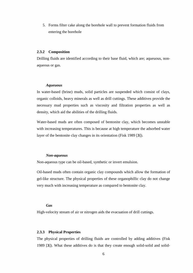
Laminar Flow
Laminar flow (streamline or viscous flow) basically occurs at low velocity and it is a
function of the viscosity. Layers of fluid move in streamlines or laminae. Figure 2.2
illustrates the flow behaviour of this viscous flow.
Figure 2.2: Illustration of laminar flow inside a drillpipe (Heriot-Watt University 2005 [4])
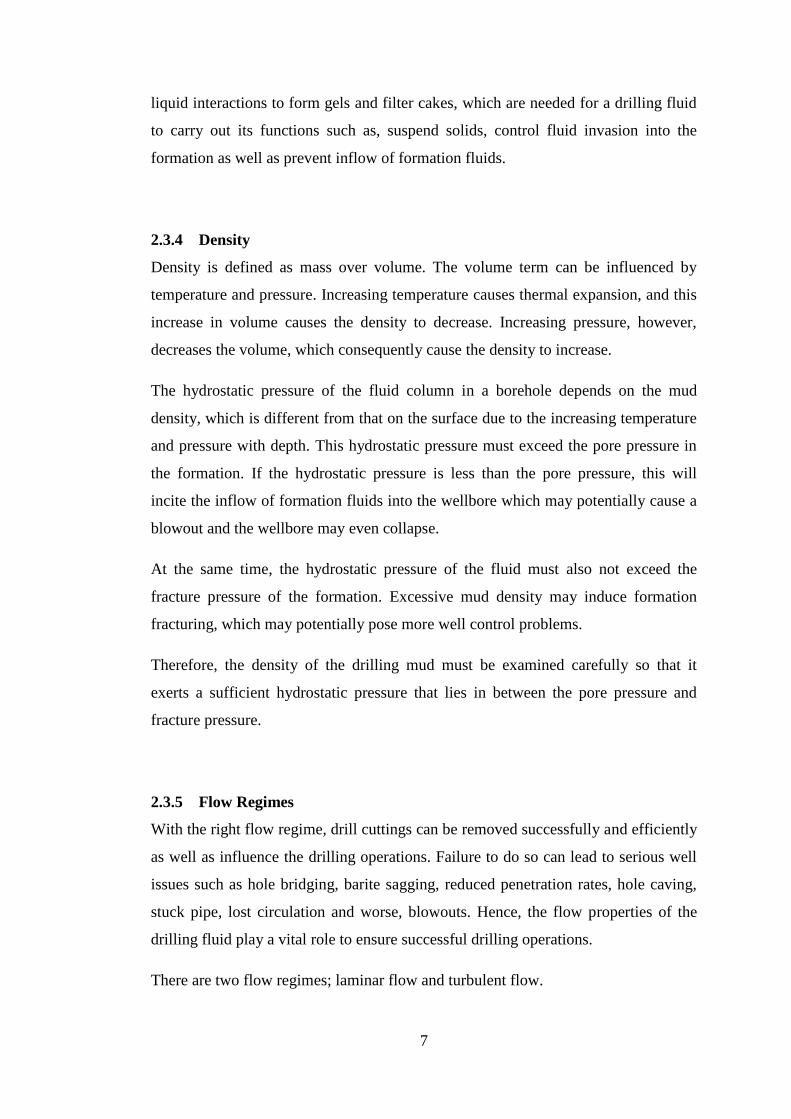
Turbulent Flow
Turbulent flow occurs at high flow velocity, which is governed by the inertial
properties and indirectly influenced by the viscous properties of the drilling fluid.
This flow is illustrated in Figure 2.3.
Figure 2.3: Illustration of turbulent flow inside a drillpipe (Heriot-Watt University 2005 [4])
Determination of Flow Regime
Figure 2.4 shows the relationship between laminar flow and turbulent flow. These
two flow regimes can be determined by using Reynolds number. Circulating fluids
through pipes is a function of pipe diameter, fluid density, viscosity and average flow
velocity, as shown in the following equation (Heriot-Watt University 2005 [4]),

9
(2.1)
Figure 2.4: Relationship between laminar flow and turbulent flow (Caenn et al 2011 [1])
As the fluid velocity is increased, the flow pattern changes from laminar to turbulent
flow and this occur at a Reynolds number of 2100 for Newtonian fluids.
2.3.6 Rheology Models
Rheology is the study of the deformation and flow of matter (Caenn et al 2011 [1]).
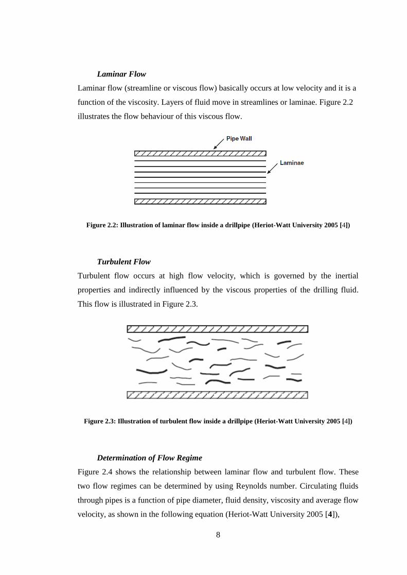
A viscous force relationship can be developed to describe a simple rheology model
from Figure 2.5 below.
(2.2)
10
The term F/A is called shear stress, , while V/L is the shear rate, .
Figure 2.5: Model of Viscous Forces in Fluids (Heriot-Watt University 2005 [4])
Bingham Plastic Model
The equation for Bingham Plastic model can be expressed in the following equation
(ASME 2004 [5]),
(2.3)
Power Law Model
Power Law can be expressed mathematically as follows (ASME 2004 [5]),
(2.4)
Herschel-Bulkley Rheological Model
Herschel-Bulkley (H-B) is widely applied in industrial standards. There are three
parameters required in this model, expressed in the following equation (ASME 2004
[5]),
(2.5)
H-B is essentially a hybrid between the Power Law and Bingham Plastic models.
When the yield stress, , is equal to the yield stress, the flow index, , which
reduces the H-B model equation to the Bingham Plastic model. Inversely, when the
yield stress is zero, , the H-B then becomes the Power Law. Figure 2.6 shows
11
the comparison between Bingham Plastic, Power Law, Newtonian and Herschel-
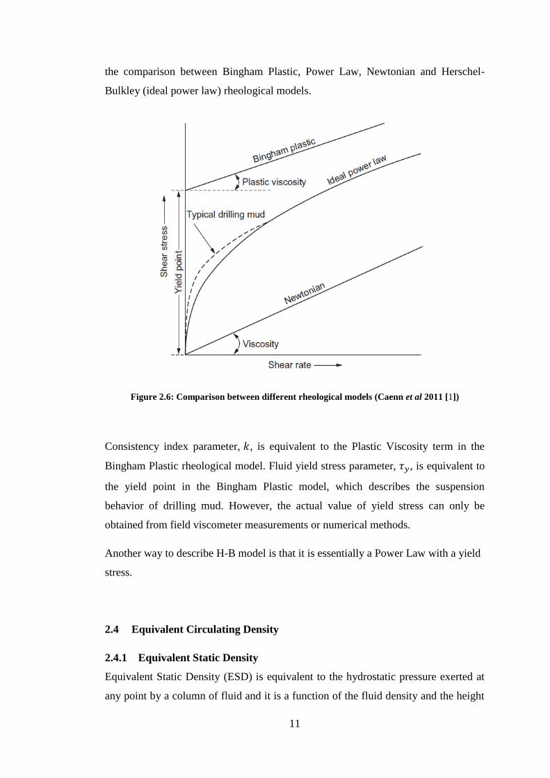
Bulkley (ideal power law) rheological models.
Figure 2.6: Comparison between different rheological models (Caenn et al 2011 [1])
Consistency index parameter, , is equivalent to the Plastic Viscosity term in the
Bingham Plastic rheological model. Fluid yield stress parameter, , is equivalent to
the yield point in the Bingham Plastic model, which describes the suspension
behavior of drilling mud. However, the actual value of yield stress can only be
obtained from field viscometer measurements or numerical methods.
Another way to describe H-B model is that it is essentially a Power Law with a yield
stress.
2.4 Equivalent Circulating Density
2.4.1 Equivalent Static Density
Equivalent Static Density (ESD) is equivalent to the hydrostatic pressure exerted at
any point by a column of fluid and it is a function of the fluid density and the height
12
of the fluid column. ESD can be mathematically expressed by the following equation
(Harris et al 2005 [6]),
(2.6)
2.4.2 Frictional Pressure Loss
Frictional pressure loss is due to contact between the drilling fluid and the walls of
conduit flow i.e. annulus and drill string. This pressure loss can be expressed by the
following equation (Harris et al 2005 [6]),
(2.7)
2.4.3 Equivalent Circulating Density
Equivalent Circulating Density (ECD) at the total depth is defined as the sum of the
ESD and the pressure loss in the annulus due to fluid flow. ECD is equivalent to the
bottomhole pressure equation expressed as a drilling fluid-density gradient as
follows:
(2.8)
2.5 Review of Finite Difference Scheme
According to Heriot-Watt University 2005 [7], finite difference technique is
essentially a simple method to approximate derivatives of a function numerically
from either point, node or block values of the function, such as, (
) (
) (
),
etc.
13
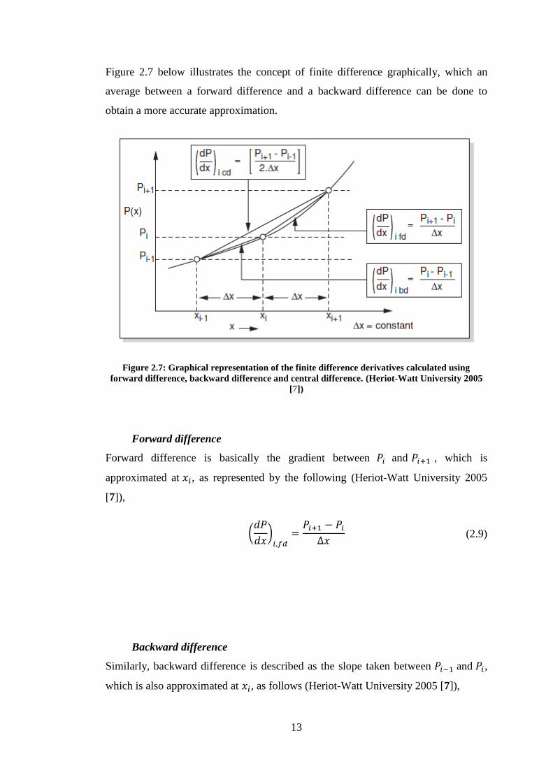
Figure 2.7 below illustrates the concept of finite difference graphically, which an
average between a forward difference and a backward difference can be done to
obtain a more accurate approximation.
Figure 2.7: Graphical representation of the finite difference derivatives calculated using
forward difference, backward difference and central difference. (Heriot-Watt University 2005
[7])
Forward difference
Forward difference is basically the gradient between and , which is
approximated at , as represented by the following (Heriot-Watt University 2005
[7]),
(
)
(2.9)
Backward difference
Similarly, backward difference is described as the slope taken between and ,
which is also approximated at , as follows (Heriot-Watt University 2005 [7]),

14
(
)
(2.10)
Central difference
From each of the two finite difference methods, approximations can be made, which,
however, introduce an error from the true values. This error can be further reduced
by introducing a Central Difference method, which is basically taking an average
between the two slopes i.e. forward difference and backward difference. This is
expressed by the following (Heriot-Watt University [7]),
(
)
*(
)
(
)
+
[
]
[
]
(2.11)
Now that we have derived finite difference for the first derivative, then according to
Heriot-Watt University 2005 [7], using the same technique, the second derivative can
be formulated as follows,
(
)
(
)
(
)
(2.12)
There are two ways to solve a finite difference problem, which are explicit method
and implicit method. These are explained briefly in the following subsections.
15
2.5.1 Explicit Solution
Explicit method is one of the techniques to solve a finite difference problem. By
taking a simplified equation as follows,
(
) (
) (2.13)
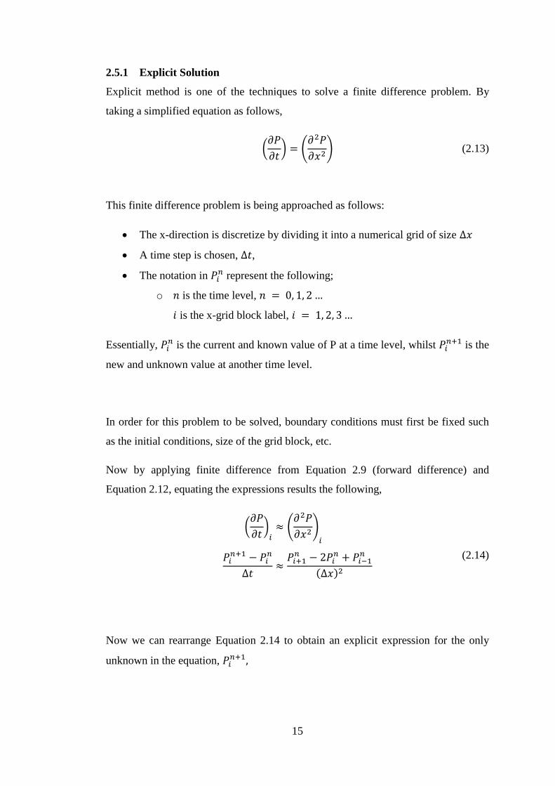
This finite difference problem is being approached as follows:
The x-direction is discretize by dividing it into a numerical grid of size
A time step is chosen, ,
The notation in represent the following;
o is the time level,
is the x-grid block label,
Essentially, is the current and known value of P at a time level, whilst
is the
new and unknown value at another time level.
In order for this problem to be solved, boundary conditions must first be fixed such
as the initial conditions, size of the grid block, etc.
Now by applying finite difference from Equation 2.9 (forward difference) and
Equation 2.12, equating the expressions results the following,
(
) (
)
(2.14)
Now we can rearrange Equation 2.14 to obtain an explicit expression for the only
unknown in the equation,
16
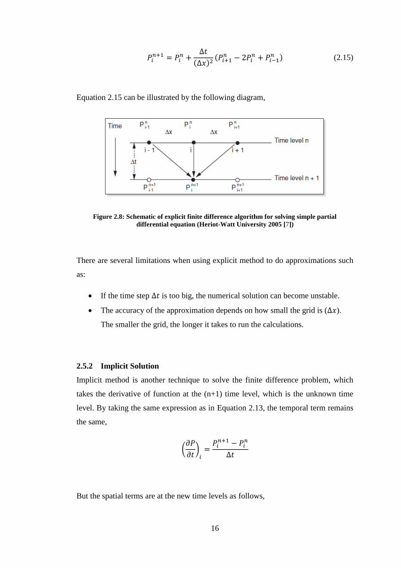
(2.15)
Equation 2.15 can be illustrated by the following diagram,
Figure 2.8: Schematic of explicit finite difference algorithm for solving simple partial
differential equation (Heriot-Watt University 2005 [7])
There are several limitations when using explicit method to do approximations such
as:
If the time step is too big, the numerical solution can become unstable.
The accuracy of the approximation depends on how small the grid is ( ).
The smaller the grid, the longer it takes to run the calculations.
2.5.2 Implicit Solution
Implicit method is another technique to solve the finite difference problem, which
takes the derivative of function at the (n+1) time level, which is the unknown time
level. By taking the same expression as in Equation 2.13, the temporal term remains
the same,
(
)
But the spatial terms are at the new time levels as follows,

17
(
)
(2.16)
By equating these two equations to obtain the following (Heriot-Watt University
2005 [7]),
(2.17)
Now, rearranging Equation 2.17 such that all the unknown terms are on one side
(LHS) while the only known term (RHS) on the other side of the equation. This is
shown below,
*
+
*
+
(2.18)
This equation can be written as follows,
(2.19)
Where,
*
+
*
+
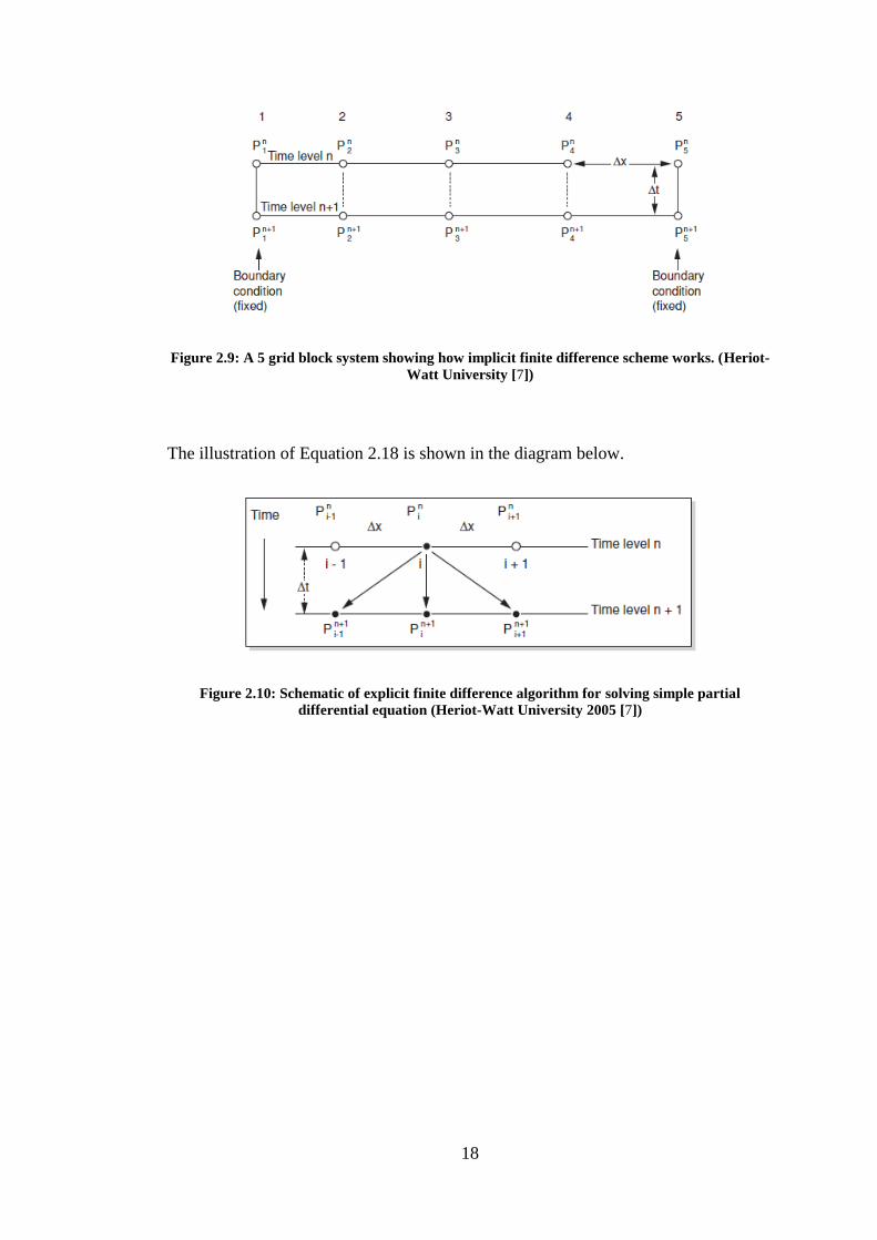
As the new time level is calculated and set to , the values of do not
change while is updated at each time step. This can be illustrated by taking a 5
grid block system as shown in Figure 2.9 below,
18
Figure 2.9: A 5 grid block system showing how implicit finite difference scheme works. (Heriot-
Watt University [7])
The illustration of Equation 2.18 is shown in the diagram below.
Figure 2.10: Schematic of explicit finite difference algorithm for solving simple partial
differential equation (Heriot-Watt University 2005 [7])
19
CHAPTER 3
METHODOLOGY
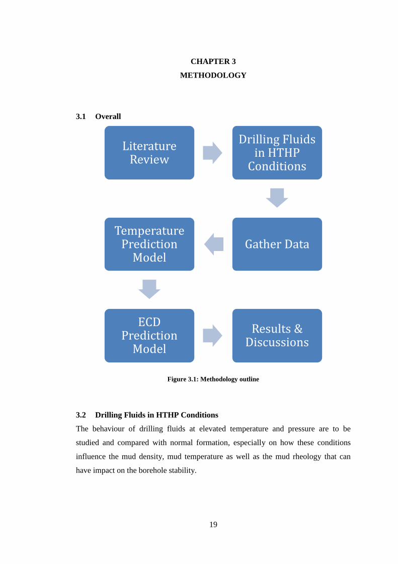
3.1 Overall
Figure 3.1: Methodology outline
3.2 Drilling Fluids in HTHP Conditions
The behaviour of drilling fluids at elevated temperature and pressure are to be
studied and compared with normal formation, especially on how these conditions
influence the mud density, mud temperature as well as the mud rheology that can
have impact on the borehole stability.
Literature Review
Drilling Fluids in HTHP
Conditions
Gather Data Temperature
Prediction Model
ECD Prediction
Model
Results & Discussions

20
3.3 Temperature Estimation
Mud temperature profile varies depending on the drilling parameters and circulation
history. In order to establish temperature profiles at different pump rates and times
from the start of circulation, a temperature simulator is required which involves
discretization process in order to solve solutions numerically. Once simulated, the
data generated can then by applied in the hydraulics calculations, which allows the
prediction of static pressure element at circulating temperature profiles.
The temperature simulator must be able to generate the temperature profiles of the
following:
Formation temperature
Fluid temperature in annulus
Fluid temperature in drillstring
How the temperature profile changes with time,
The temperature profiles in the annulus and drillstring have to be evaluated
separately to take into account the heat transfer from the formation to the drilling
fluids in the annulus, which is different from the mud temperature inside the
drillstring. Furthermore, these temperature profiles are dynamic as they vary with
time until equilibrium is reached.
From the geothermal gradient given from the Berambang-1 well data, along with
other data, this would allow the temperature profile to be plotted against depth.
There are two approaches in estimating the circulating fluid temperatures; analytical
and numerical.
Below is the list of approach to establish the wellbore temperature model:
Introduce heat flow equations
Establish heat flow diagram in the wellbore
Derive analytical solutions
Develop numerical solutions using finite difference techniques
21
3.3.1 Analytical Approach
The analytical approach involves the derivation of heat flow equations inside the
wellbore between the drillpipe, annulus and the formation.
3.3.2 Numerical Solutions
The numerical approach involves the application of finite-difference technique in
order to solve the transient heat transfer problem as proposed by Raymond 1969 [8],
using the analytical solutions derived. Boundary conditions must also be set initially.
Crank-Nicolson implicit solution will also be looked into.
3.4 ECD Model
The development of the ECD model will require in-depth study of the drilling fluids
and their rheological properties. The methodology involved building this ECD
prediction model firstly involves the prediction of downhole temperature and
pressure dependent base mud densities using empirical equations. Then, a
compositional model is used to obtain the density of mud at elevated temperature and
pressure.
The next step is to look into how rheological properties change with temperature and
pressure, where plastic viscosities and yield points at elevated conditions are
calculated using the densities obtained from the compositional model. From these
rheological properties calculations, the frictional pressure loss can be evaluated,
depending on whether the flow is laminar or turbulent.
Once the frictional pressure loss is obtained, the ECD can now be evaluated.
Sensitivity analysis can be made afterwards to see how the input parameters vary and
which of them is the most sensitive.
22
CHAPTER 4
DRILLING FLUIDS IN HTHP CONDITIONS
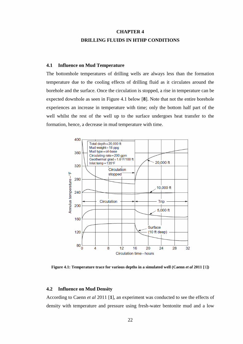
4.1 Influence on Mud Temperature
The bottomhole temperatures of drilling wells are always less than the formation
temperature due to the cooling effects of drilling fluid as it circulates around the
borehole and the surface. Once the circulation is stopped, a rise in temperature can be
expected downhole as seen in Figure 4.1 below [8]. Note that not the entire borehole
experiences an increase in temperature with time; only the bottom half part of the
well whilst the rest of the well up to the surface undergoes heat transfer to the
formation, hence, a decrease in mud temperature with time.
Figure 4.1: Temperature trace for various depths in a simulated well (Caenn et al 2011 [1])
4.2 Influence on Mud Density
According to Caenn et al 2011 [1], an experiment was conducted to see the effects of
density with temperature and pressure using fresh-water bentonite mud and a low
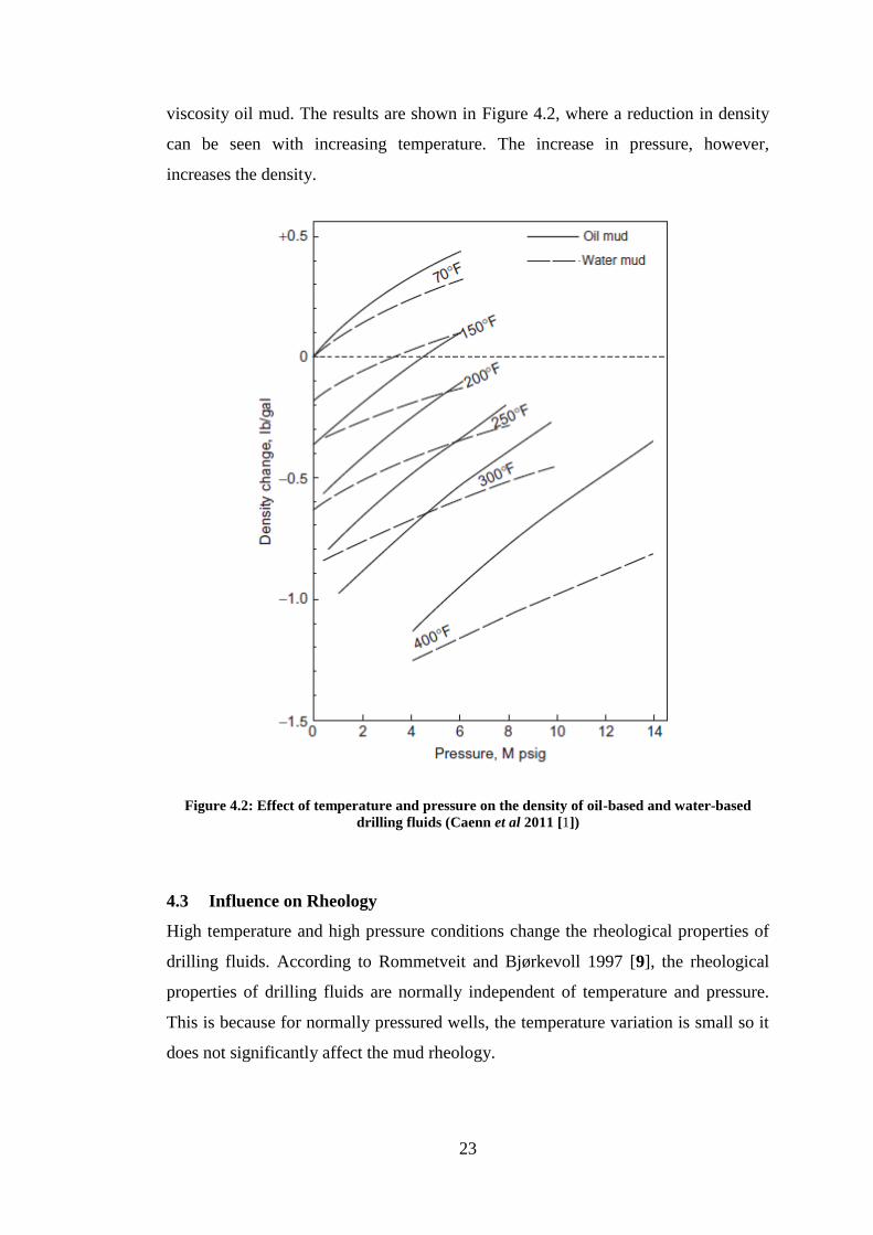
23
viscosity oil mud. The results are shown in Figure 4.2, where a reduction in density
can be seen with increasing temperature. The increase in pressure, however,
increases the density.
Figure 4.2: Effect of temperature and pressure on the density of oil-based and water-based
drilling fluids (Caenn et al 2011 [1])
4.3 Influence on Rheology
High temperature and high pressure conditions change the rheological properties of
drilling fluids. According to Rommetveit and Bjørkevoll 1997 [9], the rheological
properties of drilling fluids are normally independent of temperature and pressure.
This is because for normally pressured wells, the temperature variation is small so it
does not significantly affect the mud rheology.

24
HTHP conditions can influence the rheological properties of drilling fluids any of the
following ways (Caenn et al 2011 [1]):
4.3.1 Physical properties
The viscosity of the drilling fluid reduces as the temperature is increased.
Conversely, increase in pressure results in the increase in mud density, thus increases
the viscosity.
4.3.2 Chemical properties
Alkalinity levels in drilling fluids play some roles in how their rheological properties
change with temperature and pressure. All hydroxides react with clay minerals at
temperatures above 94°C (200°F). Low alkalinity muds have minimal impact on its
rheological properties, unlike high alkalinity muds, which may have severe effects.
4.3.3 Electrochemical properties
An increase in temperature increases the ionic activity of any electrolyte and the
solubility of any partially soluble salts that may be present in the mud. Changes in
the ionic activities affect the degree of dispersion or flocculation, which
consequently affects the rheology of mud.
The effect of water-based muds at high pressure and high temperature were studied.
The findings were such that if a suspension is completely deflocculated, the plastic
viscosity and yield point decrease with temperature up to 177°C (350°F). For a
deflocculated mud, however, the yield point increases rapidly once the temperature
exceeds boiling point of water while the plastic viscosity remains declining.
4.4 Critical Temperature
The issue with high temperature formations is that the constituents of drilling fluids
degrade with time at these elevated conditions. The rate of degradation is directly
proportional to temperature, therefore, this relationship must be taken into account
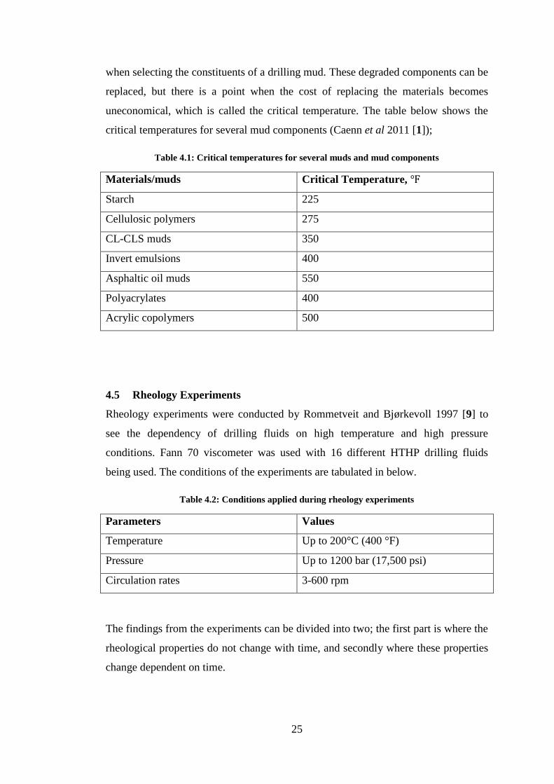
25
when selecting the constituents of a drilling mud. These degraded components can be
replaced, but there is a point when the cost of replacing the materials becomes
uneconomical, which is called the critical temperature. The table below shows the
critical temperatures for several mud components (Caenn et al 2011 [1]);
Table 4.1: Critical temperatures for several muds and mud components
Materials/muds Critical Temperature,
Starch 225
Cellulosic polymers 275
CL-CLS muds 350
Invert emulsions 400
Asphaltic oil muds 550
Polyacrylates 400
Acrylic copolymers 500
4.5 Rheology Experiments
Rheology experiments were conducted by Rommetveit and Bjørkevoll 1997 [9] to
see the dependency of drilling fluids on high temperature and high pressure
conditions. Fann 70 viscometer was used with 16 different HTHP drilling fluids
being used. The conditions of the experiments are tabulated in below.
Table 4.2: Conditions applied during rheology experiments
Parameters Values
Temperature Up to 200°C (400 °F)
Pressure Up to 1200 bar (17,500 psi)
Circulation rates 3-600 rpm
The findings from the experiments can be divided into two; the first part is where the
rheological properties do not change with time, and secondly where these properties
change dependent on time.

26
4.5.1 Time-independent properties
Increase in temperature from 50-150°C (122-302°F), the shear stress for a
high shear rate reduces significantly.
o Beyond 150°C (302°F), the shear stress increases with increasing
temperature.
For temperature below 140°C (284°F), the shear stress for a low shear rate
has less dependency on pressure and temperature.
o Temperature 140-200°C (284-392°F), the shear stress increases
rapidly.
Pressure dependence is more significant with oil-based muds (OBM)
compared to water-based muds (WBM).
o For OBM, pressure and temperature effects almost cancelled each
other out.
o For WBM, temperature has a more significant impact than pressure.
4.5.2 Time-dependent properties
Over time, high temperature and high pressure significantly increases the gel strength
of the mud.
4.6 Limitations
There are limitations with using conventional drilling fluids in HTHP wells, which is
described in the following list (Godwin et al 2011 [10]):
High ECD due to high loading of barite which creates high frictional pressure
losses during circulation in long sections.
The ability of drilling fluids to carry solids degrades at high temperature,
resulting dynamic and static barite sag.
Oil-based muds may absorb large volume of gas, and if the gas is
hydrocarbon, it can cause instability in the mud formulation, which may lead
to well control issues.

27
Recent HTHP wells have been utilizing invert emulsion drilling fluids which can
accommodate temperatures up to 315°C (600°F) (Godwin et al 2011 [10]).
Thinning agents may be added into the mud formulation in order to control the
increase in yield point with temperature, but these additives also degrade with
temperature. Of course, they can be replaced from time to time but as the rate of
degradation increases, and so as the cost.
28
CHAPTER 5
TEMPERATURE PREDICTION MODEL
As discussed previously, it is necessary to predict the temperature profile in the
wellbore as high temperature have implications on the volumetric and rheological
properties of the drilling fluids. In a HTHP well, flowing mud in the annulus absorbs
heat from the formation via conduction, resulting an increase in its temperature.
The determination of mud temperature profile in the drillpipe and annulus involves
the analysis of heat flow in the wellbore.
Firstly, the temperature profile of the formation needs to be simulated using the
given data i.e. geothermal gradient and surface temperature.
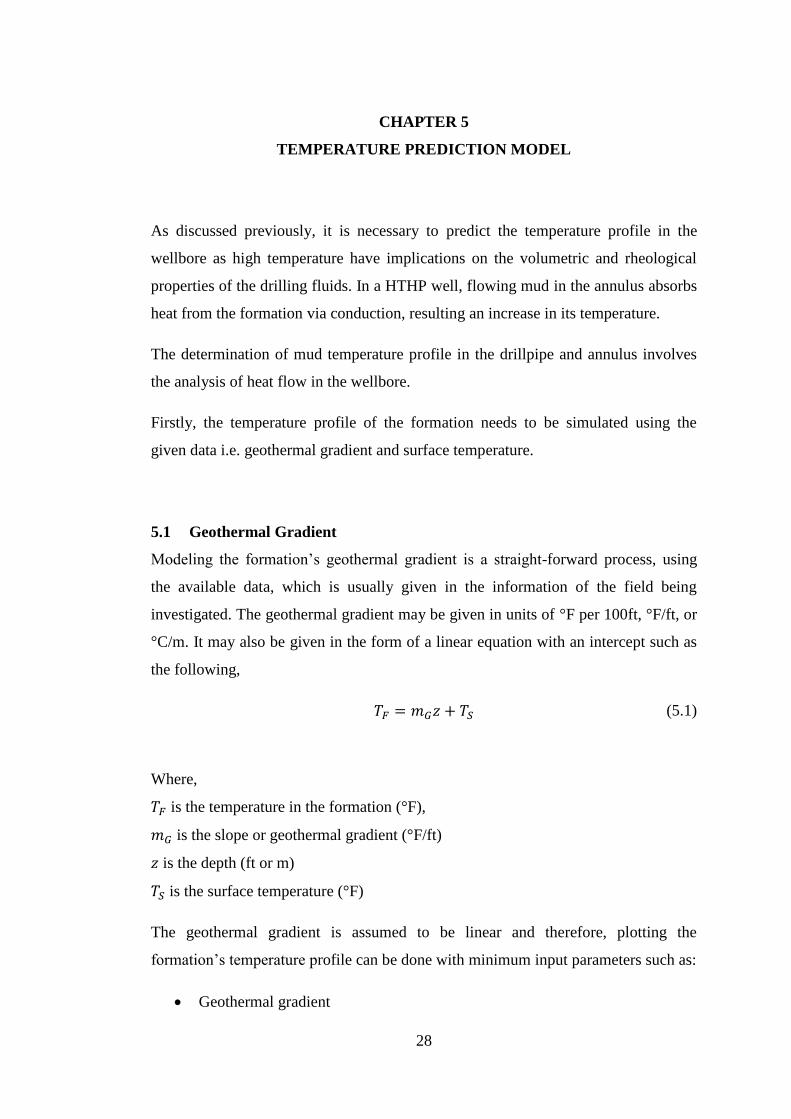
5.1 Geothermal Gradient
Modeling the formation’s geothermal gradient is a straight-forward process, using
the available data, which is usually given in the information of the field being
investigated. The geothermal gradient may be given in units of °F per 100ft, °F/ft, or
°C/m. It may also be given in the form of a linear equation with an intercept such as
the following,
(5.1)
Where,
is the temperature in the formation (°F),
is the slope or geothermal gradient (°F/ft)
is the depth (ft or m)
is the surface temperature (°F)
The geothermal gradient is assumed to be linear and therefore, plotting the
formation’s temperature profile can be done with minimum input parameters such as:
Geothermal gradient

29
Total depth
Surface temperature
5.2 Drilling Fluid Temperature
The process of drilling fluid circulation inside the wellbore involves three stages,
1. Fluid enters the drillpipe at surface and moves down the conduit
2. At the bottomhole, fluid leaves the drillpipe and enters the annulus
3. Fluid moves up the annulus and exits the conduit at surface
This process is illustrated in Figure 5.1 below.
Figure 5.1: Circulation stages inside the wellbore
5.3 Heat Transfer (Analytical)
Heat transfer can be simply expressed mathematically by the following equation,
(5.2)
30
Note that the polarity of the terms defines the direction of heat flow, which, by
convention, a positive term refers to heat gain whilst a negative term means heat loss.
By taking into account the process of drilling fluid circulation as described in Section
5.2, heat transfer can be modeled by solving equations both analytically and
numerically.
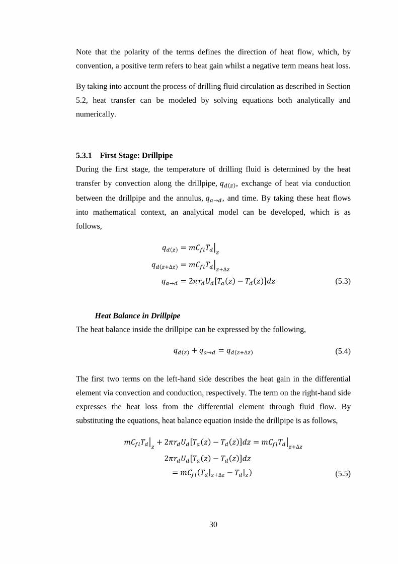
5.3.1 First Stage: Drillpipe
During the first stage, the temperature of drilling fluid is determined by the heat
transfer by convection along the drillpipe, , exchange of heat via conduction
between the drillpipe and the annulus, , and time. By taking these heat flows
into mathematical context, an analytical model can be developed, which is as
follows,
|
|
[ ] (5.3)
Heat Balance in Drillpipe
The heat balance inside the drillpipe can be expressed by the following,
(5.4)
The first two terms on the left-hand side describes the heat gain in the differential
element via convection and conduction, respectively. The term on the right-hand side
expresses the heat loss from the differential element through fluid flow. By
substituting the equations, heat balance equation inside the drillpipe is as follows,
| [ ] |
[ ]
| | (5.5)
31
Rearranging,
[ ]
(5.6)
Where,
is the radius of the drillpipe (in),
is the heat transfer coefficient between drillpipe and annulus,
is the temperature in the annulus ( ),
is the temperature in the drillpipe ( ),
is the mass flow rate of fluid (gpm),
is the density of fluid (ppg),
is the surface area of drillpipe (in2),
is the heat capacity of fluid (BTU/lb- ),
is the depth (ft)
The term on the left-hand-side describes the heat flow via conduction that occurs
between the annulus and drillpipe as a function of depth and time. The first term on
the right-hand-side describes how the temperature varies spatially i.e. in space, and
the second term, temporally i.e. in time. In other words, the first term on the right-
hand side expresses the accumulation of heat in the drillpipe (via convection of
flowing mud). The second term defines how the temperature inside the drillpipe
changes with time.
5.3.2 Second Stage: Bottomhole
The temperature of drilling fluid during the second stage, which is located at the
bottomhole, is such that the fluid temperature leaving the drillpipe is equivalent to
the fluid temperature entering the annulus.
Similarly, a mathematical model can be derived from the knowledge of this heat
flow, which is basically,
32
(5.7)
Where,
is the depth (ft),
is the total depth (ft)
5.3.3 Third Stage: Annulus
Finally, during the third stage, the mud temperature is determined by heat transfer
via convection along the annulus, heat exchange via conduction between both
formation and annulus, and annulus and drillpipe, and also time.
Again, from these heat exchanges, a mathematical model can be obtained which is
shown in the following,
|
|
[ ]
[ ] (5.8)
Heat Balance in Annulus
Using conservation of energy, heat balance in the annulus can be expressed by the
following equation,
(5.9)
The terms on the left-hand side of Equation 5.9 describes the heat gain in the
differential element in the annulus from the formation via conduction (first term) and
through bulk fluid flow via convection (second term). The first two terms on the
right-hand side is where heat escapes the differential element via conduction from
the annulus to the drillpipe, and via convection through bulk fluid flow, respectively.
By substituting the terms from Equation 5.8, the heat balance equation inside the
annulus is obtained as follows,

33
[ ] |
[ ] |
| |
[ ]
[ ] (5.10)
Where,
is the radius of the annulus (in),
Rearranging Equation 5.10,
[ ]
[ ] (5.11)
The first two terms on the left-hand side basically describes the heat exchange
between the formation and annulus, and between the annulus and drillpipe through
conduction along the walls of the annulus and drillpipe. The first term on the right-
hand side describes the heat loss due to fluid flow, whilst the second term describes
the heat flow along the annulus via convection.
Flowing fluid temperature in the wellbore can be modeled separately for each of its
flow conduit i.e. drillpipe and annulus, which is a function of the well depth and
circulation rate and time. The flow of fluid, in this case, is down the drillpipe and up
the annulus. The reverse flow can also be modeled according to Kabir et al [11], but
this is not considered in this project. This forward circulation model involves energy
balance i.e. heat transfer between the formation and the fluid in both conduits
(drillpipe and annulus).
There are a few assumptions put in place for this model to work, which are:
Heat transfer is steady-state in the wellbore (drillpipe and annulus)
Transient heat transfer occurs in the formation
34
Transient heat transfer in the radial direction can be expressed using a partial
differential equation as follows,
(
)
(5.12)
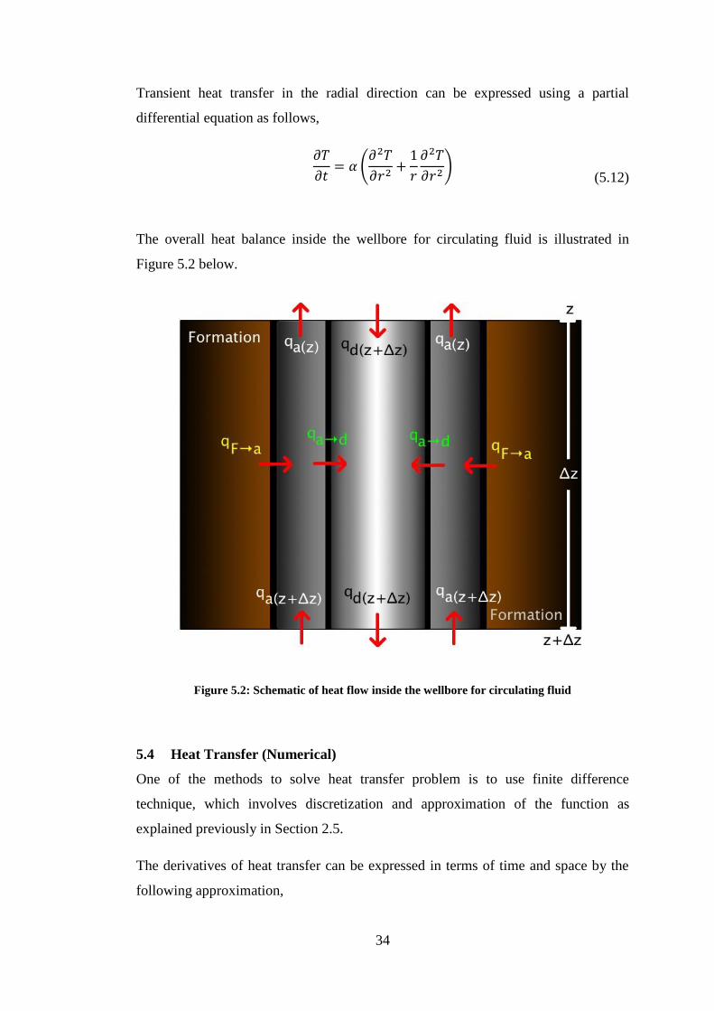
The overall heat balance inside the wellbore for circulating fluid is illustrated in
Figure 5.2 below.
Figure 5.2: Schematic of heat flow inside the wellbore for circulating fluid
5.4 Heat Transfer (Numerical)
One of the methods to solve heat transfer problem is to use finite difference
technique, which involves discretization and approximation of the function as
explained previously in Section 2.5.
The derivatives of heat transfer can be expressed in terms of time and space by the
following approximation,
35
| ⁄
(5.13)
| ⁄
(5.14)
The second derivatives can then be approximated by taking the differences of the
first derivative, as shown in the following,
|
| ⁄
|
(5.15)
5.4.1 Conservation of Energy in the Wellbore and Formation
Harris [6] showed that the heat exchange inside the drillpipe can be expressed using
conservation of energy by the following equation,
[ ]
(5.16)
Where,
is the radius of the drillpipe (in),
is the heat transfer coefficient between drillpipe and annulus (),
is the temperature in the annulus ( ),
is the temperature in the drillpipe ( ),
is the temperature of the formation ( ),
is the mass flow rate of fluid (gpm),
is the density of fluid (ppg),
is the heat capacity of fluid (BTU/lb- ),
is the depth (ft)

36
Consequently, the equation that describes the heat transfer inside the annulus is as
follows,
[ ]
[ ]
(5.17)
Where,
is the radius of the annulus (in),
is the heat transfer coefficient between drillpipe and annulus (),
And finally, the temperature in the formation is expressed as follows,
(
)
(5.18)
Where,
is the formation transmissivity (
⁄ ),
is the formation conductivity,
is the formation density,
is the formation heat transfer coefficient
The heat flow in the formation is assumed to only occur in the radial direction.
Between the boundary of the annulus and formation, the heat exchange is expressed
by the following,
37
[ ]
*
+
(5.19)
5.4.2 Discretization of Heat Flow Equations
A finite difference grid is developed in order to solve how the heat transfer
propagates along and the formation and the wellbore.
The temperatures in the drillpipe, annulus and the formation can be expressed by the
following equations,
Where,
is the depth co-ordinate,
is the radial co-ordinate, and
is the time co-ordinate
There are two ways to discretize the heat flow inside the wellbore; explicit or
implicit finite difference technique. These are further explained in thorough details in
the following.
5.5 Explicit Method
Using explicit finite difference method which have been explained in the Literature
Review (See Section 2.5.1), the heat exchange inside the drillpipe, Equation 5.16,
can be discretized as follows,
38
*
+
*
+
*
+
(5.20)
The next step is to rearrange Equation 5.20 such that the unknown term, , is
on the left-hand side, while the rest of the known terms on the right-hand side of the
equation, as follows,
*
( )+
*
( )+
(5.21)
Similarly, Equation 5.17, which describes the heat exchange inside the annulus, can
be discretized for the purpose of solving using a finite difference technique as shown
below,
39
*
+
*
+
*
+
*
+
(5.22)
Again, Equation 5.22 can be rearranged such that the known and the unknown terms
are on the opposite side of the equation. Likewise, the only unknown term in this
explicit method is whilst the rest,
, ,
, ,
and
are known. This is shown in the following,
40
( )
* ( )
+
(5.23)
The issue with explicit finite difference technique is the accuracy of the
approximation as it has time step limitations i.e. if the time step is too big, the
prediction of the numerical solution can become unstable. Furthermore, the more
refined the grid is i.e. smaller , the more accurate the approximation is. This may
take a long time to calculate.
41
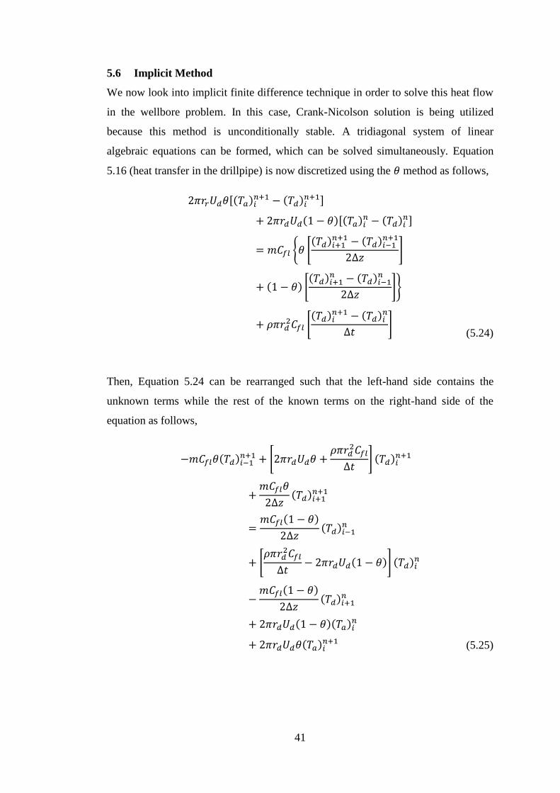
5.6 Implicit Method
We now look into implicit finite difference technique in order to solve this heat flow
in the wellbore problem. In this case, Crank-Nicolson solution is being utilized
because this method is unconditionally stable. A tridiagonal system of linear
algebraic equations can be formed, which can be solved simultaneously. Equation
5.16 (heat transfer in the drillpipe) is now discretized using the method as follows,
[
]
[
]
, *
+
*
+-
*
+
(5.24)
Then, Equation 5.24 can be rearranged such that the left-hand side contains the
unknown terms while the rest of the known terms on the right-hand side of the
equation as follows,
*
+
*
+
(5.25)
42
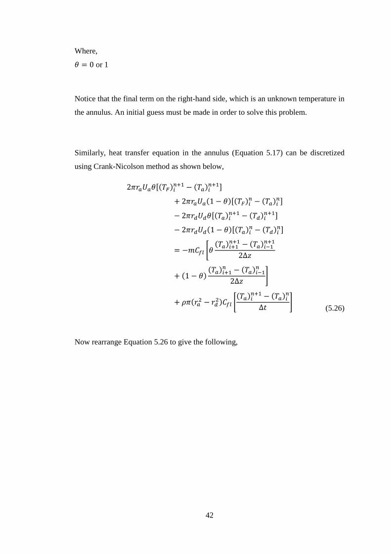
Where,
or 1
Notice that the final term on the right-hand side, which is an unknown temperature in
the annulus. An initial guess must be made in order to solve this problem.
Similarly, heat transfer equation in the annulus (Equation 5.17) can be discretized
using Crank-Nicolson method as shown below,
[
]
[
]
[
]
[
]
*
+
*
+
(5.26)
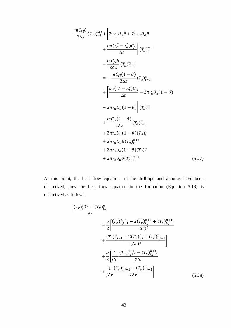
Now rearrange Equation 5.26 to give the following,
43
*
+
*
+
(5.27)
At this point, the heat flow equations in the drillpipe and annulus have been
discretized, now the heat flow equation in the formation (Equation 5.18) is
discretized as follows,
*
+
*
+
(5.28)
44
Rearranging Equation 5.28 gives,
[
]
[
]
[
]
[
]
[
]
[
]
(5.29)
5.7 Boundary Conditions
In order to solve these equations, boundary conditions must be set. At the surface,
the temperature in the drillpipe is equivalent to the surface temperature of the pipe
inlet. At the bottomhole, the temperature in the drillpipe is equivalent to the
temperature in the annulus.
The boundary conditions can applied mathematically on this model is as follows,
At the drillpipe inlet, ,
( )
Where,
is the temperature of fluid in the drillpipe inlet at the surface.
At the bottomhole, ,
Now, a heat balance equation at the bottomhole can be derived as follows,
45
[ ]
[ ]
(5.30)
5.7.1 Drillpipe Boundary Conditions
In the drillpipe, , Equation 5.30 can be discretized using Crank-Nicolson
scheme as follows,
[
]
[
]
[
]
[
]
*
+
(5.31)
Rearranging Equation 5.31 results the following,
*
+
*
+
(5.32)
5.7.2 Annulus Boundary Conditions
Now in the annulus, , similarly Equation 5.30 can be discretized to obtain the
following,
46
*( )
+
*( )
+
[
]
[
]
*
+
(5.33)
Rearranging Equation 5.33 gives,
*
+
*
+
( )
( )
(5.34)
5.7.3 Formation Boundary Conditions
The boundary condition at the interface between the formation and the annulus can
be expressed in the following equation,
(5.35)
Equation 5.35 is now discretized as follows,
(5.36)
47
Rearrange Equation 5.36 for each time step of n and n+1,
[
]
(5.37)
[
]
(5.38)
48
CHAPTER 6
ECD PREDICTION MODEL
6.1 Static Mud Density
Kutasov 1999 [12] presented an empirical equation of state for drilling muds and
brines, which allows the prediction of fluid densities at downhole conditions, which
is valid for either water or oil-based drilling fluids or brine;
[
] (6.1)
where,
is the temperature ( ,
is the pressure (psig),
is the international standard temperature ( or ),
is the fluid density (ppg),
is the fluid density at standard conditions (ppg),
is the isothermal compressibility,
and are constant coefficients
The coefficients for Equation 6.1 are listed in the Appendix (Table 10.1).
6.2 Compositional Model
The knowledge of drilling fluid compositions, mud density at surface conditions as
well as the density of its individual liquid component at elevated conditions would
allow the prediction of mud density at elevated temperature and pressure. In order to
simulate the density of drilling fluid inside the wellbore, a compositional mass
balance model was proposed (Peters et al 1990 [13]). The following equations derive
this model.
At the surface temperature and pressure, the volume, , and mass, , of the drilling
fluid are expressed as follows,
49
(6.2)
Where,
are the volumes of oil, water, solids and chemical components in a
drilling fluid
(6.3)
Where,
are the densities of oil, water, solids and chemical components in a
drilling fluid
After the drilling mud has been exposed to the high temperature and high pressure
inside the wellbore, volume changes are expected in the oil and water components of
the mud. These volume changes are expressed as,
(6.4)
Where,
is the new density of components subject to HTHP
Since solids have low compressibility, they are assumed to have negligible volume
changes when subject to these temperature and pressure. Now, a new mud volume
can be modeled as,
(6.5)
Now, the drilling fluid density elevated at high temperature and pressure can be
expressed using Equation 6.3 and Equation 6.5 as follows,
(6.6)

50
By taking the volume of fractions of mud where the sum of volume fractions, , of
each of the component is equivalent to 1, Equation 6.6 can be expressed below,
(6.7)
Substituting Equation 6.4,
(
) (
)
(6.8)
The assumption of this model is that any change in density of drilling fluid caused by
temperature and pressure conditions is caused by the volumetric behavior of its fluid
constituents, and also solid constituents are assumed to have negligible
compressibility and thermal expansion.
6.3 Rheological Model
It is necessary to model how the rheological properties of the drilling fluid change
with temperature and pressure. In this case, only Bingham-Plastic rheological model
is applied.
6.3.1 Plastic Viscosity
Plastic viscosity of oil-based drilling fluids at elevated temperature and pressure can
be obtained by normalizing with the viscosity of the base oil (Politte 1985 [14]). This
is valid for any oil-based drilling fluid. This is expressed in the following equation,
(6.9)
Where,
is the mud plastic viscosity at elevated temperature and pressure,
is the mud plastic viscosity at surface conditions,
51
is the base oil plastic viscosity at elevated temperature and pressure,
is the base oil plastic viscosity at surface conditions.
Politte 1985 [14] obtained an empirical expression of base oil viscosity as a function
of temperature and pressure from the analysis of diesel oil-based drilling fluid, which
is as follows,
(
⁄ ) (6.10)
The values of constants can be found in Table 10.2 in the
Appendix section. The value for is obtained from Equation 6.13.
6.3.2 Yield Point
Yield point at elevated temperature and pressure is also evaluated. However, a
rheological study (Politte 1985 [14]) has shown that pressure has little effect on the
yield point. Therefore, pressure effect can be ignored. An empirical equation has
been developed from the same analysis of diesel oil to evaluate the yield point, ,
which is valid for temperatures from 90 to 300°F.
(6.11)
Where,
is the yield point at surface conditions,
are constants
The values of these constants can be found in Table 10.3 in the Appendix section.
6.4 ECD Model
Using the compositional model to predict the mud density as explained previously
(See Section 6.2). One of the main assumptions of this model is that any change in
52
density of drilling fluid caused by temperature and pressure conditions is due to the
volumetric behavior of its fluid constituents. In most cases, oil and water are the
main constituents of drilling mud. Similar to Equation 6.8, this model can be
expressed by the following equation,
(
) (
)
(6.12)
where,
is the mud density at reference condition
is the mud density at elevated temperature and pressure
are oil and water densities at reference conditions
are oil and water densities at elevated temperature and pressure
are volume fractions of oil and water
By studying the volumetric behaviour of the each of the fluid constituent, its
respective density can be determined.
6.4.1 Volumetric Behaviour of Oil Phase
An empirical equation is used to describe the volumetric behavior of the oil phase,
which is developed by Politte 1985 [14], and this equation can be expressed as the
following:
(6.13)
where,
is temperature (°F),
is pressure (psi),
are constants with the following values,
The values of these constants can be found in Table 10.4 in the Appendix.
53
6.4.2 Volumetric Behaviour of Water Phase
Politte 1985 [14] also developed another empirical equation to describe the
volumetric behavior of the water phase as follows:
(6.14)
Where,
is temperature (°F),
is pressure (psi),
are constants with the following values,
Constants values can be found in Table 10.5 in the Appendix section.
6.4.3 Evaluating Frictional Pressure Loss
As discussed previously in the Literature Review (See Section 2), in order to
determine the ECD, the frictional pressure loss must first be determined in the
wellbore.
Apparent Viscosity
The Bingham Plastic model can be used to calculate the apparent viscosity,
separately in the drillpipe and the annulus, using the following equation,
Drillpipe,
(6.15)
Annulus,
(6.16)

54
Frictional Pressure Loss
Reynolds equation (Equation 2.1) can be used to determine whether the flow is
laminar or turbulent. The flow is classified as laminar when the calculated Reynolds
number is equivalent to or less than 2100 (Heriot-Watt University 2005 [4]).
If this is the case, the frictional pressure loss in each drillpipe and annulus, can be
evaluated using the following equations,
Drillpipe,
(
) (6.17)
Annulus
(
) (6.18)
Where,
is the inner annular wall (in)
is the outer annular wall (in)
If the flow is classified as turbulent (for Reynolds number > 2100), the fanning
friction factor, , is calculated using Colebrook Equation which is expressed in the
following,
√ ( √ ) (6.19)
55
Equation 2.7 is then used to calculate the frictional pressure loss for turbulent flow,
which is as follows,
6.5 Evaluating ECD
As discussed in the Literature Review (see Section 2.4), ECD can be evaluated using
Equation 2.8 which is basically the sum of the equivalent static density (ESD) and
the equivalent fluid density due to pressure loss during flow.
The ESD can be found from the pressure exerted by the static mud column i.e. no
circulation is taking place. The effects of temperature and pressure on the density and
rheological properties of the drilling fluid must be taken into account and this is
being done by evaluating the density using the compositional model (Equation 6.12).
The base mud densities in this model are functions of temperature and pressure and
with the circulating fluid temperatures simulated from the previous section, the
temperature and pressure dependent density is now evaluated.
The pressure loss can be calculated in two ways and it depends on whether the fluid
flowing in a laminar or turbulent fashion, which can be determined from Reynolds
number. For the case of a laminar flow, the plastic viscosity and the yield point of the
fluid can be both evaluated empirically using Equation 6.10 and Equation 6.11,
combined with the recently obtained values of the temperature and pressure
dependent densities. Now, using Equation 6.17 and Equation 6.18, the pressure loss
in both flow conduits i.e. drillpipe and annulus, can now be evaluated.
For the case of a turbulent flow, the pressure loss can be determined directly using
Equation 2.7 after calculating the friction factor from Colebrook Equation (Equation
6.19).
With that, the ECD for each depth can now be evaluated and then plotted.
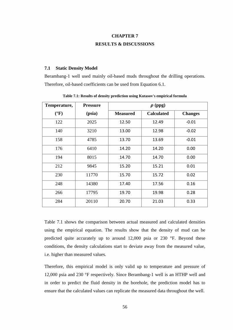
56
CHAPTER 7
RESULTS & DISCUSSIONS
7.1 Static Density Model
Berambang-1 well used mainly oil-based muds throughout the drilling operations.
Therefore, oil-based coefficients can be used from Equation 6.1.
Table 7.1: Results of density prediction using Kutasov's empirical formula
Temperature,
(°F)
Pressure
(psia)
(ppg)
Measured Calculated Changes
122 2025 12.50 12.49 -0.01
140 3210 13.00 12.98 -0.02
158 4785 13.70 13.69 -0.01
176 6410 14.20 14.20 0.00
194 8015 14.70 14.70 0.00
212 9845 15.20 15.21 0.01
230 11770 15.70 15.72 0.02
248 14380 17.40 17.56 0.16
266 17795 19.70 19.98 0.28
284 20110 20.70 21.03 0.33
Table 7.1 shows the comparison between actual measured and calculated densities
using the empirical equation. The results show that the density of mud can be
predicted quite accurately up to around 12,000 psia or 230 °F. Beyond these
conditions, the density calculations start to deviate away from the measured value,
i.e. higher than measured values.
Therefore, this empirical model is only valid up to temperature and pressure of
12,000 psia and 230 °F respectively. Since Berambang-1 well is an HTHP well and
in order to predict the fluid density in the borehole, the prediction model has to
ensure that the calculated values can replicate the measured data throughout the well.
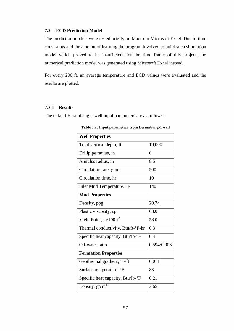
57
7.2 ECD Prediction Model
The prediction models were tested briefly on Macro in Microsoft Excel. Due to time
constraints and the amount of learning the program involved to build such simulation
model which proved to be insufficient for the time frame of this project, the
numerical prediction model was generated using Microsoft Excel instead.
For every 200 ft, an average temperature and ECD values were evaluated and the
results are plotted.
7.2.1 Results
The default Berambang-1 well input parameters are as follows:
Table 7.2: Input parameters from Berambang-1 well
Well Properties
Total vertical depth, ft 19,000
Drillpipe radius, in 6
Annulus radius, in 8.5
Circulation rate, gpm 500
Circulation time, hr 10
Inlet Mud Temperature, °F 140
Mud Properties
Density, ppg 20.74
Plastic viscosity, cp 63.0
Yield Point, lb/100ft2 58.0
Thermal conductivity, Btu/ft-°F-hr 0.3
Specific heat capacity, Btu/lb-°F 0.4
Oil-water ratio 0.594/0.006
Formation Properties
Geothermal gradient, °F/ft 0.011
Surface temperature, °F 83
Specific heat capacity, Btu/lb-°F 0.21
Density, g/cm3 2.65
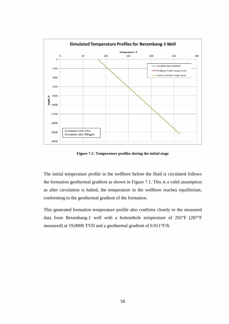
58
Figure 7.1: Temperature profiles during the initial stage
The initial temperature profile in the wellbore before the fluid is circulated follows
the formation geothermal gradient as shown in Figure 7.1. This is a valid assumption
as after circulation is halted, the temperature in the wellbore reaches equilibrium,
conforming to the geothermal gradient of the formation.
This generated formation temperature profile also confirms closely to the measured
data from Berambang-1 well with a bottomhole temperature of 292°F (287°F
measured) at 19,000ft TVD and a geothermal gradient of 0.011°F/ft.
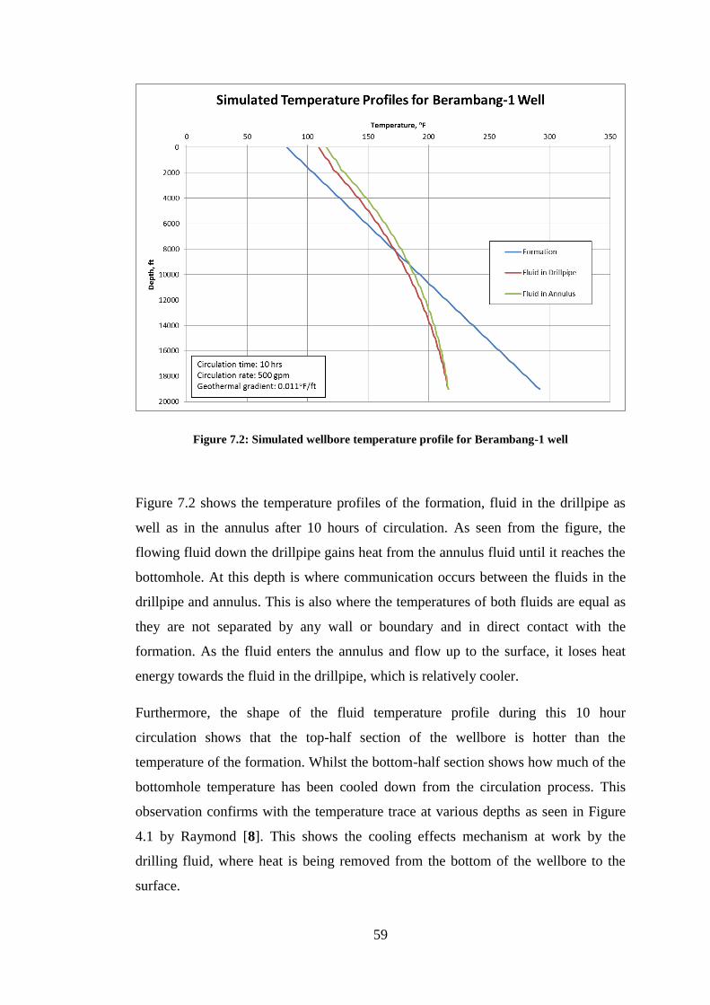
59
Figure 7.2: Simulated wellbore temperature profile for Berambang-1 well
Figure 7.2 shows the temperature profiles of the formation, fluid in the drillpipe as
well as in the annulus after 10 hours of circulation. As seen from the figure, the
flowing fluid down the drillpipe gains heat from the annulus fluid until it reaches the
bottomhole. At this depth is where communication occurs between the fluids in the
drillpipe and annulus. This is also where the temperatures of both fluids are equal as
they are not separated by any wall or boundary and in direct contact with the
formation. As the fluid enters the annulus and flow up to the surface, it loses heat
energy towards the fluid in the drillpipe, which is relatively cooler.
Furthermore, the shape of the fluid temperature profile during this 10 hour
circulation shows that the top-half section of the wellbore is hotter than the
temperature of the formation. Whilst the bottom-half section shows how much of the
bottomhole temperature has been cooled down from the circulation process. This
observation confirms with the temperature trace at various depths as seen in Figure
4.1 by Raymond [8]. This shows the cooling effects mechanism at work by the
drilling fluid, where heat is being removed from the bottom of the wellbore to the
surface.

60
Over time, as the heat from the formation is absorbed by the fluid and circulated out
to the surface, the temperature in the upper part section of the wellbore becomes
higher than the formation temperature. This phenomenon observed is due to the rate
at which the absorbed heat in the fluid being circulated out is faster than the rate of
heat exchange between the formation and the fluids in the flow conduits. In other
words, heat is being evacuated faster than it is being transferred between mediums.
At the bottomhole of depth 19,000ft, the fluid temperature has reduced to 216°F after
10 hours of circulation.
Figure 7.3: Simulated equivalent circulating density for Berambang-1 well
From the temperature profiles generated in Figure 7.2, the ECD was evaluated and
plotted as shown in Figure 7.3. As seen from the results, the equivalent circulating
density decreases with depth. The reason for this behaviour is that as the fluid flows
down the drillpipe, the temperature increases. With increasing temperature, the fluid
constituents experience thermal expansion, which consequently, reduces the ECD.
The ECD at the bottomhole is calculated to be 22.34 ppg.
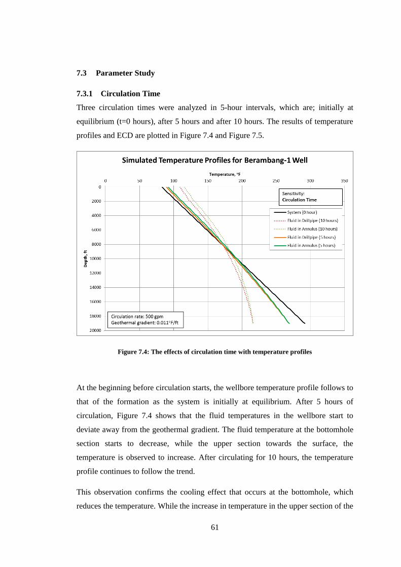
61
7.3 Parameter Study
7.3.1 Circulation Time
Three circulation times were analyzed in 5-hour intervals, which are; initially at
equilibrium (t=0 hours), after 5 hours and after 10 hours. The results of temperature
profiles and ECD are plotted in Figure 7.4 and Figure 7.5.
Figure 7.4: The effects of circulation time with temperature profiles
At the beginning before circulation starts, the wellbore temperature profile follows to
that of the formation as the system is initially at equilibrium. After 5 hours of
circulation, Figure 7.4 shows that the fluid temperatures in the wellbore start to
deviate away from the geothermal gradient. The fluid temperature at the bottomhole
section starts to decrease, while the upper section towards the surface, the
temperature is observed to increase. After circulating for 10 hours, the temperature
profile continues to follow the trend.
This observation confirms the cooling effect that occurs at the bottomhole, which
reduces the temperature. While the increase in temperature in the upper section of the
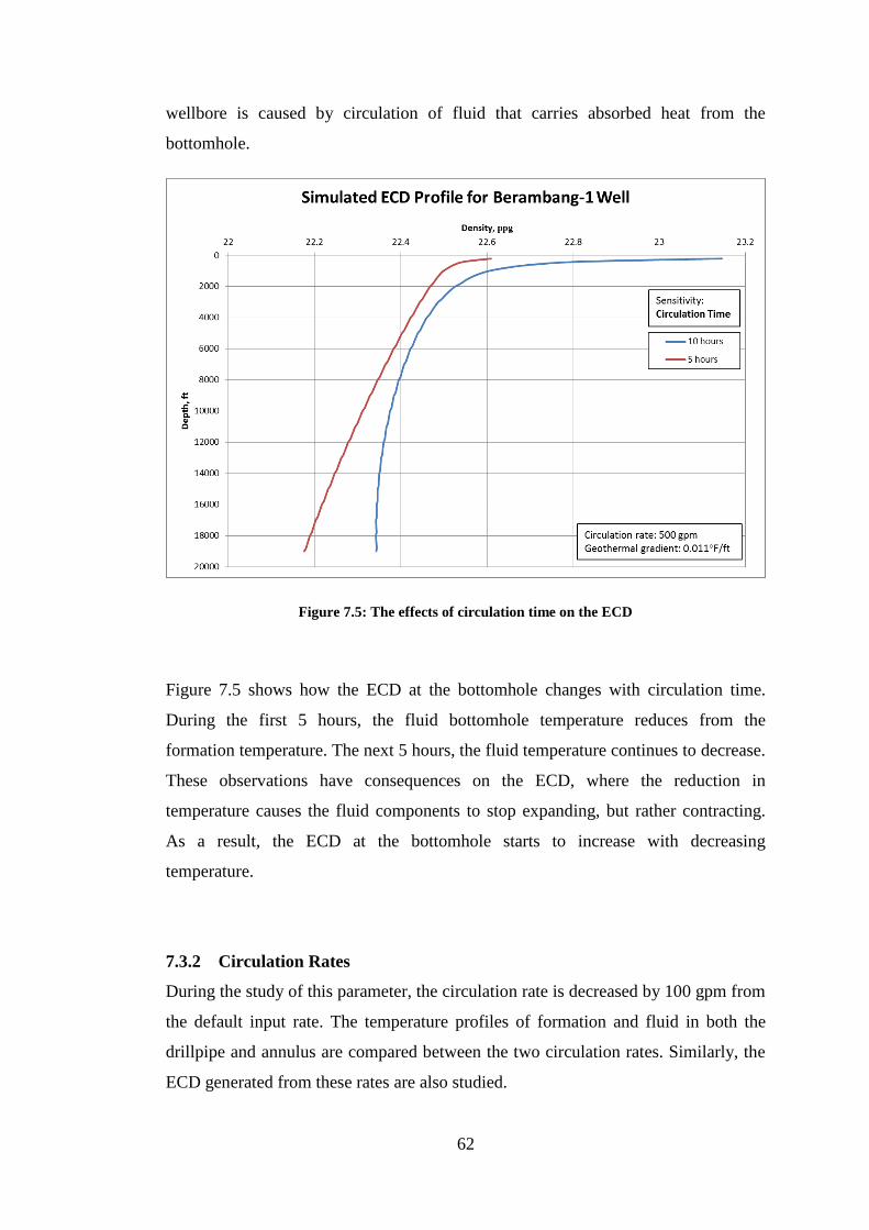
62
wellbore is caused by circulation of fluid that carries absorbed heat from the
bottomhole.
Figure 7.5: The effects of circulation time on the ECD
Figure 7.5 shows how the ECD at the bottomhole changes with circulation time.
During the first 5 hours, the fluid bottomhole temperature reduces from the
formation temperature. The next 5 hours, the fluid temperature continues to decrease.
These observations have consequences on the ECD, where the reduction in
temperature causes the fluid components to stop expanding, but rather contracting.
As a result, the ECD at the bottomhole starts to increase with decreasing
temperature.
7.3.2 Circulation Rates
During the study of this parameter, the circulation rate is decreased by 100 gpm from
the default input rate. The temperature profiles of formation and fluid in both the
drillpipe and annulus are compared between the two circulation rates. Similarly, the
ECD generated from these rates are also studied.
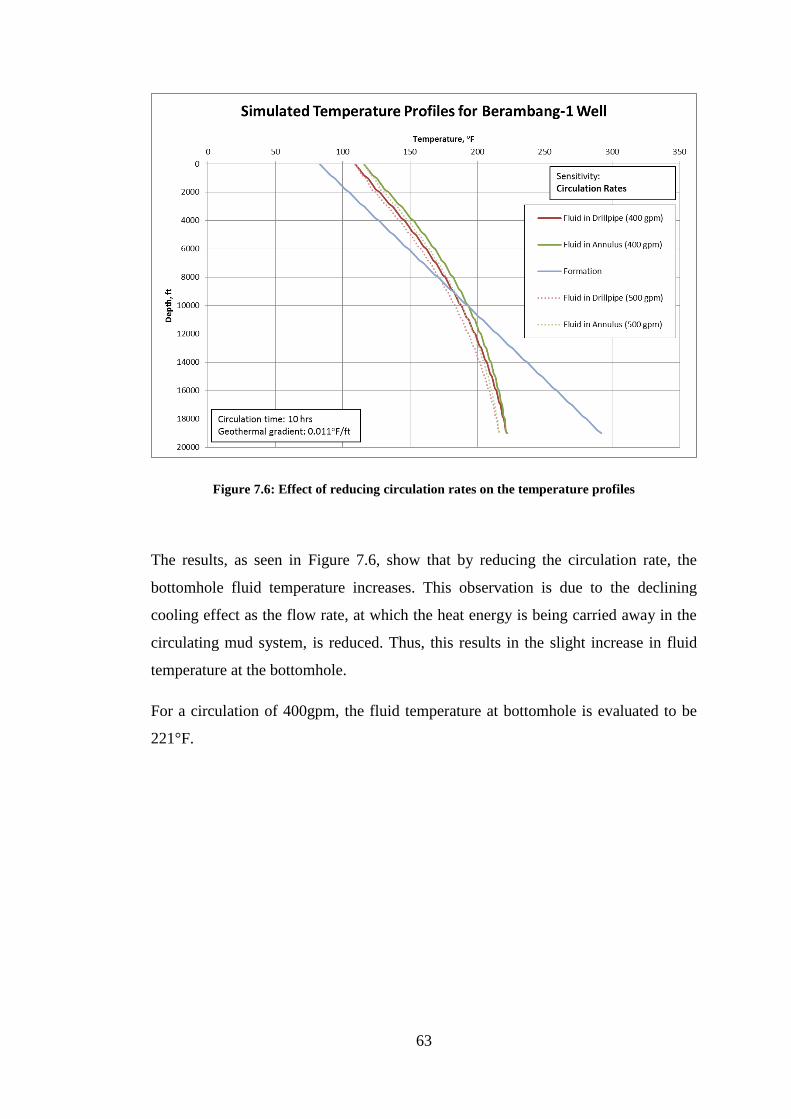
63
Figure 7.6: Effect of reducing circulation rates on the temperature profiles
The results, as seen in Figure 7.6, show that by reducing the circulation rate, the
bottomhole fluid temperature increases. This observation is due to the declining
cooling effect as the flow rate, at which the heat energy is being carried away in the
circulating mud system, is reduced. Thus, this results in the slight increase in fluid
temperature at the bottomhole.
For a circulation of 400gpm, the fluid temperature at bottomhole is evaluated to be
221°F.
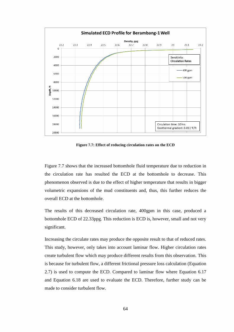
64
Figure 7.7: Effect of reducing circulation rates on the ECD
Figure 7.7 shows that the increased bottomhole fluid temperature due to reduction in
the circulation rate has resulted the ECD at the bottomhole to decrease. This
phenomenon observed is due to the effect of higher temperature that results in bigger
volumetric expansions of the mud constituents and, thus, this further reduces the
overall ECD at the bottomhole.
The results of this decreased circulation rate, 400gpm in this case, produced a
bottomhole ECD of 22.33ppg. This reduction is ECD is, however, small and not very
significant.
Increasing the circulate rates may produce the opposite result to that of reduced rates.
This study, however, only takes into account laminar flow. Higher circulation rates
create turbulent flow which may produce different results from this observation. This
is because for turbulent flow, a different frictional pressure loss calculation (Equation
2.7) is used to compute the ECD. Compared to laminar flow where Equation 6.17
and Equation 6.18 are used to evaluate the ECD. Therefore, further study can be
made to consider turbulent flow.
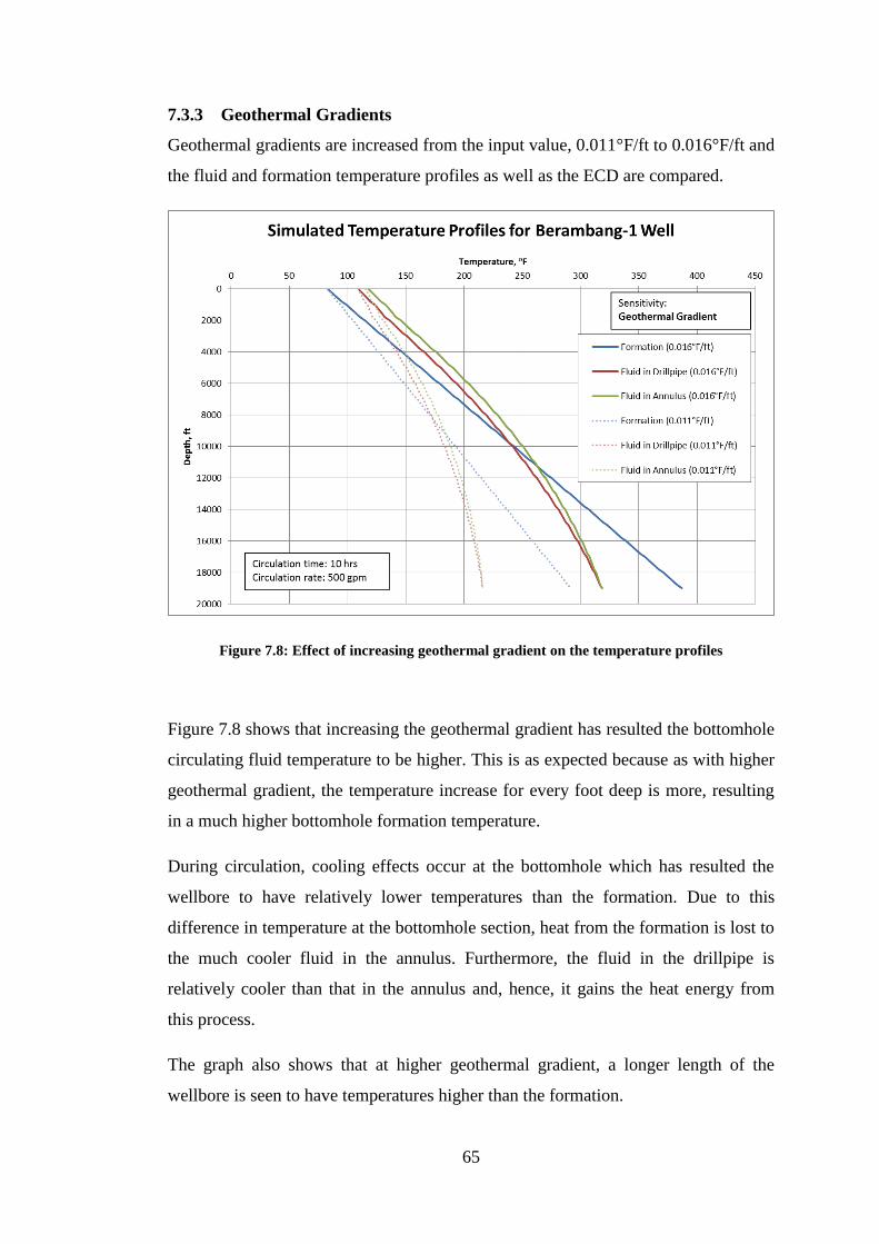
65
7.3.3 Geothermal Gradients
Geothermal gradients are increased from the input value, 0.011°F/ft to 0.016°F/ft and
the fluid and formation temperature profiles as well as the ECD are compared.
Figure 7.8: Effect of increasing geothermal gradient on the temperature profiles
Figure 7.8 shows that increasing the geothermal gradient has resulted the bottomhole
circulating fluid temperature to be higher. This is as expected because as with higher
geothermal gradient, the temperature increase for every foot deep is more, resulting
in a much higher bottomhole formation temperature.
During circulation, cooling effects occur at the bottomhole which has resulted the
wellbore to have relatively lower temperatures than the formation. Due to this
difference in temperature at the bottomhole section, heat from the formation is lost to
the much cooler fluid in the annulus. Furthermore, the fluid in the drillpipe is
relatively cooler than that in the annulus and, hence, it gains the heat energy from
this process.
The graph also shows that at higher geothermal gradient, a longer length of the
wellbore is seen to have temperatures higher than the formation.
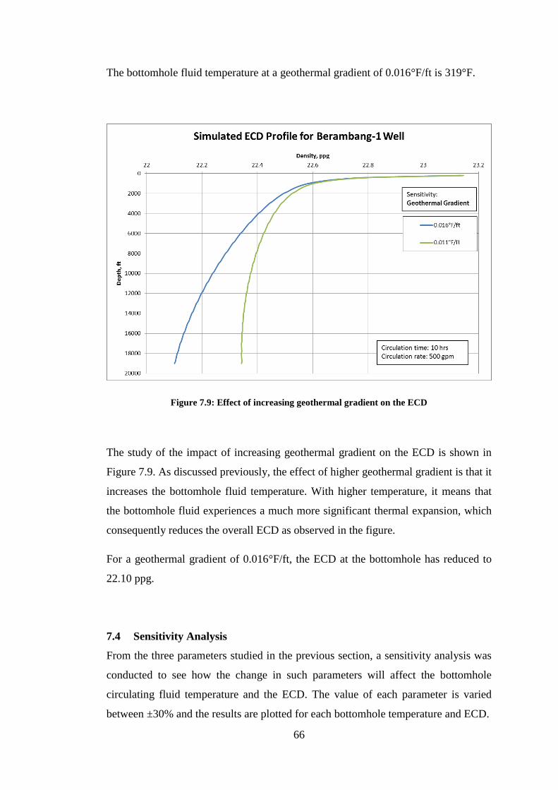
66
The bottomhole fluid temperature at a geothermal gradient of 0.016°F/ft is 319°F.
Figure 7.9: Effect of increasing geothermal gradient on the ECD
The study of the impact of increasing geothermal gradient on the ECD is shown in
Figure 7.9. As discussed previously, the effect of higher geothermal gradient is that it
increases the bottomhole fluid temperature. With higher temperature, it means that
the bottomhole fluid experiences a much more significant thermal expansion, which
consequently reduces the overall ECD as observed in the figure.
For a geothermal gradient of 0.016°F/ft, the ECD at the bottomhole has reduced to
22.10 ppg.
7.4 Sensitivity Analysis
From the three parameters studied in the previous section, a sensitivity analysis was
conducted to see how the change in such parameters will affect the bottomhole
circulating fluid temperature and the ECD. The value of each parameter is varied
between ±30% and the results are plotted for each bottomhole temperature and ECD.
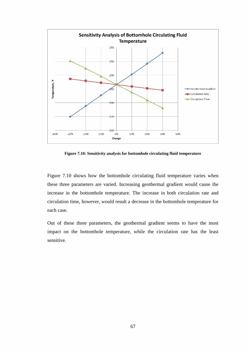
67
Figure 7.10: Sensitivity analysis for bottomhole circulating fluid temperature
Figure 7.10 shows how the bottomhole circulating fluid temperature varies when
these three parameters are varied. Increasing geothermal gradient would cause the
increase in the bottomhole temperature. The increase in both circulation rate and
circulation time, however, would result a decrease in the bottomhole temperature for
each case.
Out of these three parameters, the geothermal gradient seems to have the most
impact on the bottomhole temperature, while the circulation rate has the least
sensitive.
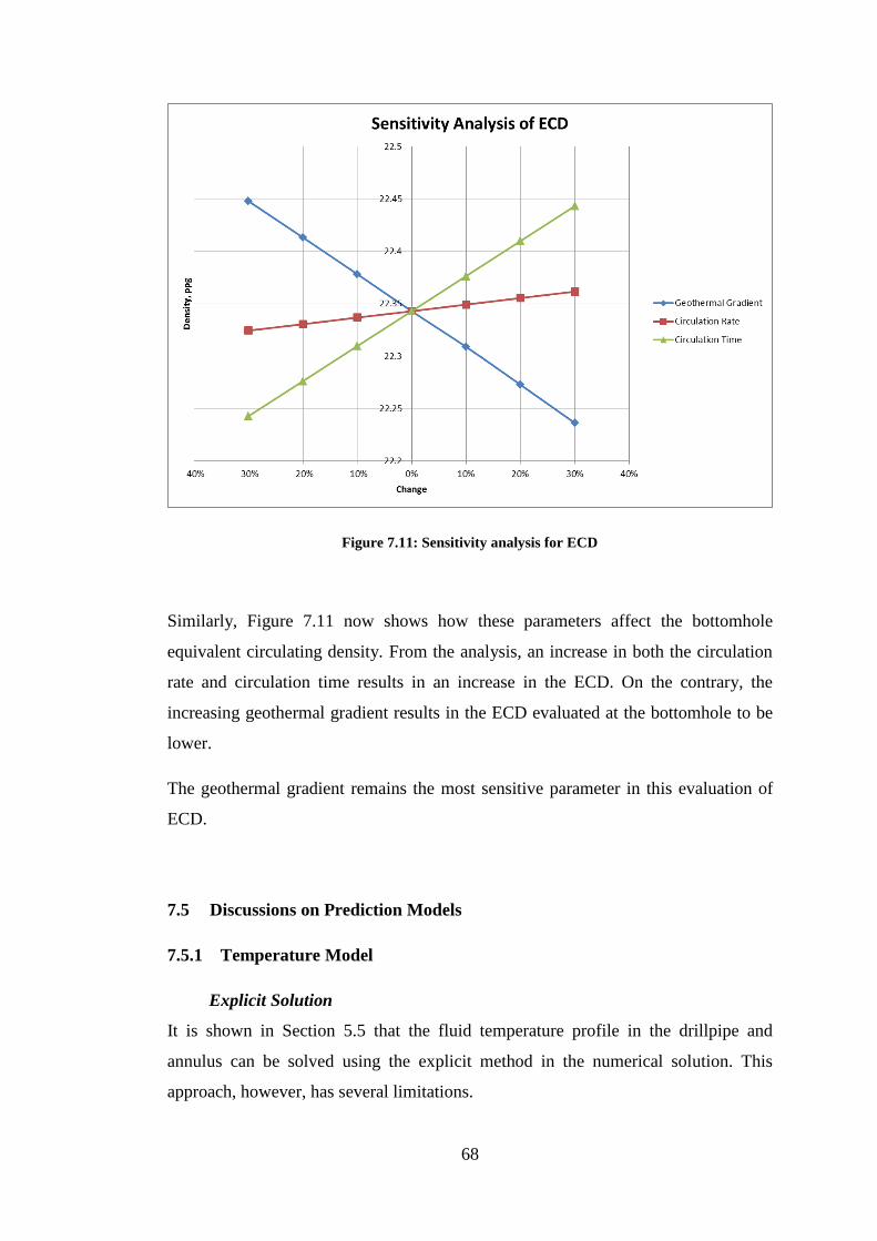
68
Figure 7.11: Sensitivity analysis for ECD
Similarly, Figure 7.11 now shows how these parameters affect the bottomhole
equivalent circulating density. From the analysis, an increase in both the circulation
rate and circulation time results in an increase in the ECD. On the contrary, the
increasing geothermal gradient results in the ECD evaluated at the bottomhole to be
lower.
The geothermal gradient remains the most sensitive parameter in this evaluation of
ECD.
7.5 Discussions on Prediction Models
7.5.1 Temperature Model
Explicit Solution
It is shown in Section 5.5 that the fluid temperature profile in the drillpipe and
annulus can be solved using the explicit method in the numerical solution. This
approach, however, has several limitations.
69
Having a large time-step may cause the solution fail to converge, thus, the numerical
approximations may become unstable. The accuracy of the approximation also
depends on the size of the grid. The finer the grid, the more accurate the solution
becomes but the drawback having fine grids is that the calculations can take a long
time, thus, inefficient.
Crank-Nicolson Scheme
Crank-Nicolson scheme allows the numerical solutions to be approximated and the
beauty of this approach is that it is unconditionally stable. This means that choosing
a time step is no longer an issue. Compared to the explicit method, where choosing a
time-step plays a major role ensuring a stable solution.
Applying this implicit technique requires solving a set of simultaneous equations
which can be done in the matrix form.
With this technique, the prediction model should be able to simulate circulating fluid
temperature profile both in the drillpipe and the annulus over a specified time, which
can be specified by the user.
7.5.2 ECD Model
ECD can be determined by evaluating the circulating mud density in the wellbore as
well as the frictional pressure loss. Together with the numerical approximations of
the fluid temperature profile, the ECD can be modeled, thus, predicted.
Evaluating the density requires the development of a compositional model which is
shown in Section 6.2, where the change in density when subjected to high
temperature and pressure are due to the change in volumes of the fluids constituents
in the drilling fluid. This compositional model takes into account mainly water and
oil components as the rest of the solid constituents do not change very much in terms
of volume and, thus, density with temperature and pressure.
70
7.6 Determining Well Control Issues from ECD
The results from the ECD prediction model show that during circulation, the
bottomhole experiences a temperature drop with time and circulation rate. This
decrease in temperature results in the cooling of the drilling fluid. During this
process, the fluid constituents (mainly liquid) start to contract in volume and as a
result, the overall ECD is increased.
This increase in circulating density may pose problem to the well control as HTHP
formation is known to have narrow margins between the pore pressure and fracture
pressure, there is a risk of fracturing the formation and thus, lost circulation.
The results of the ECD prediction model also show that the temperature increase per
depth in the formation, in other words geothermal gradient, is very sensitive. This
means that well control problems are further complicated with heterogeneous HTHP
formations, which have non-linear geothermal gradients. This is because if the
bottomhole formation has a higher geothermal gradient compared to the formation
above it, the bottomhole has a higher temperature than anticipated. With higher
formation temperature, the circulating fluid temperature also remains higher than
expected even after the cooling effects.
High temperature causes the fluid constituents to experience thermal expansions,
which consequently reduces the overall ECD. The combination of reduced ECD and
narrow pore pressure and fracture pressure in HTHP formation results in the risk of
formation fluid influx into the wellbore, thus, forming a kick.
71
CHAPTER 8
CONCLUSIONS
The outcome of this project can be ended with the following conclusions:
HTHP wells have narrow pore pressure and fracture pressure margins,
therefore it is vitally important to ensure the right mud weight and proper
mud constituents selected to prevent well control problems.
At high temperatures, components of drilling fluids degrade faster resulting
mud failure where the drilling fluid unable to fulfill its primary functions.
Crank-Nicolson scheme and Thomas algorithm are unconditionally stable and
efficient for the numerical solution technique to predict fluid temperature
profile in the wellbore
Fluid density that is dependent on temperature and pressure can be evaluated
using compositional model.
Increasing circulation rates causes the bottomhole fluid temperature to
decrease due to cooling effects. The same effect is seen with increasing
circulation time.
The most sensitive parameter that affects ECD is geothermal gradient.
Therefore, it is important to accurately profile the formation temperature as
accurately as possible, especially heterogeneous formations.
It is possible to expect well control issues from the ECD predicted in
conjunction with the pore and fracture pressure plot as well as an accurate
geothermal gradient.
Choosing the right mud constituents that can withstand high temperatures and
pressures is vitally important to prevent or minimize well control issues.
8.1 Practical Applications
At the moment, an ECD prediction model does not have a practical value in terms of
applications in actual drilling operations in the oil and gas industry. This is because
during the drilling operations in the real world, tackling well control problems is

72
done by an “action-reaction” mechanism. Basically, well control issues are remedied
only once they have been encountered during the operation itself.
Having an ECD prediction model that able to predict well control issues anticipated
by a well, for now, is more towards educational purposes rather than industrial
applications.
8.2 Recommendations
There are several things that can be pointed out of this study, which can be used to
further improve the findings in the future.
8.2.1 High-Temperature Drilling Fluids
Recent HTHP wells have been utilizing invert emulsion drilling fluids which can
accommodate temperatures up to 315°C (600°F).
8.2.2 Temperature Model
The temperature model outlined in this project does not take into account the water
depth. The consequence of a well running through sea water would usually cause
temperature to decrease at a profile. As the HTHP well data used is actually an
offshore well, there are some discrepancies with the simulated geothermal gradient
and, thus, fluid temperature profiles. Hence, studying this temperature effects in sea
water may help improve the reliability of this prediction model.
The prediction of the fluid temperatures inside the wellbore can be further improved
by taking into account the heat transfer that occurs along the drillpipe wall as well as
the annulus wall (casing). This is because heat conducts faster in solid, especially
metal or steel.
Further improvement of this temperature model can be made by being able to
simulate fluid temperatures during other drilling operations such as tripping and
workovers.
73
8.2.3 ECD Prediction Model
Only Bingham-Plastic rheological model is being used to create the prediction
model. There is room for improvement by considering other rheological model such
as Power Law and especially Herschel-Bulkley, which is widely used in the industry.
Furthermore, the prediction model is only able to calculate the ECD based on
laminar flow properties. Further study can be made to understand how would the
ECD change and compare during turbulent flow.
8.2.4 Sensitivity Analysis
During the prediction of fluid temperature profile in the wellbore, sensitivity analysis
were carried out to study how the parameters such as circulation time, geothermal
gradient, circulation rates can affect the bottomhole fluid temperatures during
circulation. Further sensitivity analysis could be carried to study the effects of other
input parameters such as the inlet mud temperature, thermal conductivity of mud and
formation.
This sensitivity analysis can also be further expanded to understand how the volume
fractions of drilling fluid components and other parameters in the ECD
compositional model can affect the ECD profile.
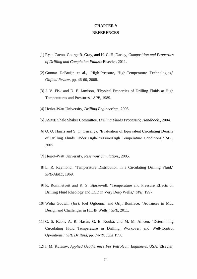
74
CHAPTER 9
REFERENCES
[1] Ryan Caenn, George R. Gray, and H. C. H. Darley, Composition and Properties
of Drilling and Completion Fluids.: Elsevier, 2011.
[2] Gunnar DeBruijn et al., "High-Pressure, High-Temperature Technologies,"
Oilfield Review, pp. 46-60, 2008.
[3] J. V. Fisk and D. E. Jamison, "Physical Properties of Drilling Fluids at High
Temperatures and Pressures," SPE, 1989.
[4] Heriot-Watt University, Drilling Engineering., 2005.
[5] ASME Shale Shaker Committee, Drilling Fluids Processing Handbook., 2004.
[6] O. O. Harris and S. O. Osisanya, "Evaluation of Equivalent Circulating Density
of Drilling Fluids Under High-Pressure/High Temperature Conditions," SPE,
2005.
[7] Heriot-Watt University, Reservoir Simulation., 2005.
[8] L. R. Raymond, "Temperature Distribution in a Circulating Drilling Fluid,"
SPE-AIME, 1969.
[9] R. Rommetveit and K. S. Bjørkevoll, "Temperature and Pressure Effects on
Drilling Fluid Rheology and ECD in Very Deep Wells," SPE, 1997.
[10] Woha Godwin (Jnr), Joel Ogbonna, and Oriji Boniface, "Advances in Mud
Design and Challenges in HTHP Wells," SPE, 2011.
[11] C. S. Kabir, A. R. Hasan, G. E. Kouba, and M. M. Ameen, "Determining
Circulating Fluid Temperature in Drilling, Workover, and Well-Control
Operations," SPE Drilling, pp. 74-79, June 1996.
[12] I. M. Kutasov, Applied Geothermics For Petroleum Engineers. USA: Elsevier,
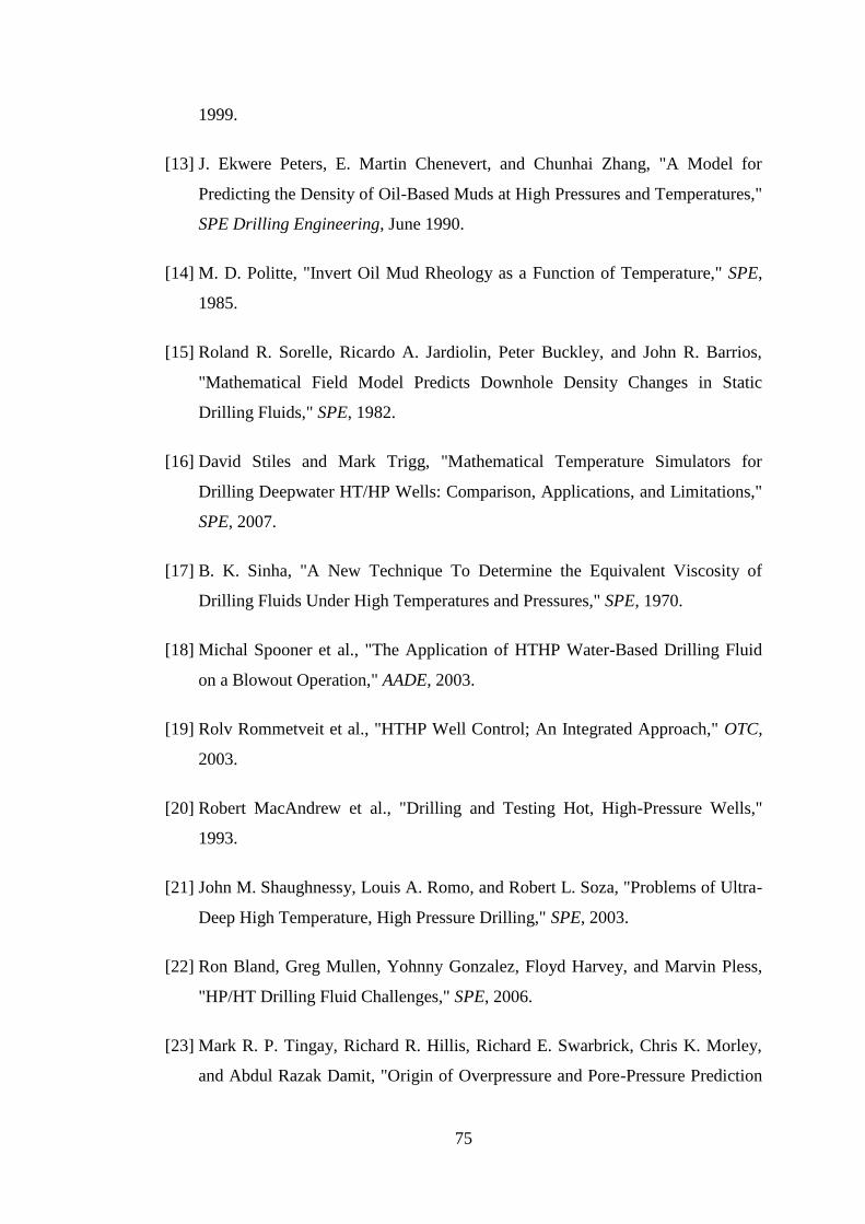
75
1999.
[13] J. Ekwere Peters, E. Martin Chenevert, and Chunhai Zhang, "A Model for
Predicting the Density of Oil-Based Muds at High Pressures and Temperatures,"
SPE Drilling Engineering, June 1990.
[14] M. D. Politte, "Invert Oil Mud Rheology as a Function of Temperature," SPE,
1985.
[15] Roland R. Sorelle, Ricardo A. Jardiolin, Peter Buckley, and John R. Barrios,
"Mathematical Field Model Predicts Downhole Density Changes in Static
Drilling Fluids," SPE, 1982.
[16] David Stiles and Mark Trigg, "Mathematical Temperature Simulators for
Drilling Deepwater HT/HP Wells: Comparison, Applications, and Limitations,"
SPE, 2007.
[17] B. K. Sinha, "A New Technique To Determine the Equivalent Viscosity of
Drilling Fluids Under High Temperatures and Pressures," SPE, 1970.
[18] Michal Spooner et al., "The Application of HTHP Water-Based Drilling Fluid
on a Blowout Operation," AADE, 2003.
[19] Rolv Rommetveit et al., "HTHP Well Control; An Integrated Approach," OTC,
2003.
[20] Robert MacAndrew et al., "Drilling and Testing Hot, High-Pressure Wells,"
1993.
[21] John M. Shaughnessy, Louis A. Romo, and Robert L. Soza, "Problems of Ultra-
Deep High Temperature, High Pressure Drilling," SPE, 2003.
[22] Ron Bland, Greg Mullen, Yohnny Gonzalez, Floyd Harvey, and Marvin Pless,
"HP/HT Drilling Fluid Challenges," SPE, 2006.
[23] Mark R. P. Tingay, Richard R. Hillis, Richard E. Swarbrick, Chris K. Morley,
and Abdul Razak Damit, "Origin of Overpressure and Pore-Pressure Prediction
76
in the Baram Province, Brunei," AAPG, 2009.
[24] P. Isambourg, B. T. Anfinsen, and C. Marken, "Volumetric Behavior of Drilling
Muds at High Pressure and High Temperature," SPE, 1996.

77
CHAPTER 10
APPENDICES
10.1 Introduction
Figure 10.1: Project schedule
10.2 ECD Model Prediction
Table 10.1: Coefficients of constants for static fluid density
Mud base
Water-base 10.770 3.3815 -2.3489 -4.2366
Water-base 13.684 3.2976 -1.7702 -5.2126
Water-base 18.079 3.0296 -1.3546 -4.4144
Oil-base 11.020 6.5146 -4.3414 1.4144
Oil-base 14.257 6.0527 -3.0027 -0.5156
Oil-base 18.049 5.1951 -2.9637 0.7460
Sodium chloride 8.591 3.9414 -1.6008 -4.5254
Sodium chloride 9.886 3.0519 -2.1967 -1.4840
Calcium bromide 15.227 1.3506 -2.4383 -0.3618
Table 10.2: Empirical constants for equation calculating base oil viscosity
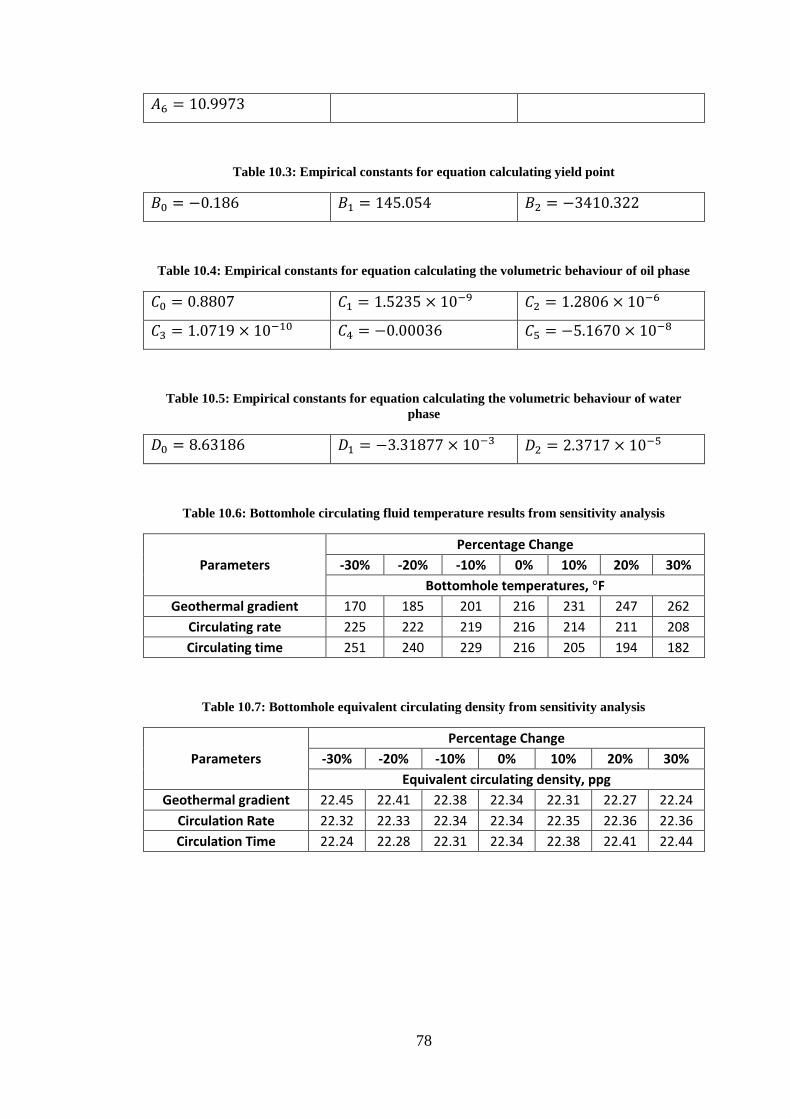
78
Table 10.3: Empirical constants for equation calculating yield point
Table 10.4: Empirical constants for equation calculating the volumetric behaviour of oil phase
Table 10.5: Empirical constants for equation calculating the volumetric behaviour of water
phase
Table 10.6: Bottomhole circulating fluid temperature results from sensitivity analysis
Parameters
Percentage Change
-30% -20% -10% 0% 10% 20% 30%
Bottomhole temperatures, °F
Geothermal gradient 170 185 201 216 231 247 262
Circulating rate 225 222 219 216 214 211 208
Circulating time 251 240 229 216 205 194 182
Table 10.7: Bottomhole equivalent circulating density from sensitivity analysis
Parameters
Percentage Change
-30% -20% -10% 0% 10% 20% 30%
Equivalent circulating density, ppg
Geothermal gradient 22.45 22.41 22.38 22.34 22.31 22.27 22.24
Circulation Rate 22.32 22.33 22.34 22.34 22.35 22.36 22.36
Circulation Time 22.24 22.28 22.31 22.34 22.38 22.41 22.44