ROOTS YOGA220 Cambridge Street .Burlington, MA 01803 ‘ROOTS ON THE ROAD’ ROOTS YOGA

Determining the Roots ofNon-Linear Equations
– Part I –
Prof. Dr. Florian Rupp
German University of Technology in Oman (GUtech)Introduction to Numerical Methods for ENG & CS
(Mathematics IV)
Spring Term 2016

Exercise Session

Reviewing the highlights from last time(1/ 2)
Prof. Dr. Florian Rupp GUtech 2016: Numerical Methods – 3 / 44
Computer Exercise
Computer exerciseUse MATLAB’s function parabolic to solve the heat equation heat equationut(t, x, y) = ∆u(t, x, y) on a square geometry −1 ≤ x, y ≤ 1 with “discontin-uous” initial data u(0, x, y) = 1 on the disk x2 + y2 < 0.42, and u(0, x, y) = 0otherwise as well as zero Dirichlet boundary conditions. Plot the solution attimes 0, 0.1, 20.
[p,e,t] = initmesh(’squareg’);
[p,e,t] = refinemesh(’squareg’,p,e,t);
u0 = zeros(size(p,2),1);
ix = find(sqrt(p(1,:).∧2+p(2,:).∧2)<0.4);
u0(ix) = ones(size(ix));
tlist = linspace(0,0.1,20);
u1 = parabolic(u0,tlist,’squareb1’,p,e,t,1,0,0,1);

Reviewing the highlights from last time(2/ 2)
Prof. Dr. Florian Rupp GUtech 2016: Numerical Methods – 4 / 44
Reviewing the highlights from last time
1D Schrodinger EquationThe 1D time dependent Schodinger Equation basically reads as iut(t, z) =k∆u(t, z) + V (z) · u(t, z). Give its FTCS approximation.
1D Finite Difference ApproximationUse Taylor approximation to determine a 1D finite difference approximation ofthe derivative u(x) · ux(x).

Introduction & Todays Scope

The Catenary
Prof. Dr. Florian Rupp GUtech 2016: Numerical Methods – 6 / 44
The catenary models an idealized hanging chain or cable that is subject to itsown weight when supported only at its ends. The catenary is described by
y(x) = a · cosh(x
a
)
,
where the parameter a depends on the chain’s or cable’s material properties.
�����
���
�����
�� ��

Determining the parameter a
Prof. Dr. Florian Rupp GUtech 2016: Numerical Methods – 7 / 44
Assume, you we are interested in the material parameter a for a hanging cablebetween two supporting points that are 100 m apart from each other.
By experiments we know that in this situation the maximal displacement is 10m, as sketched on the previous slide.
Plugged into the catenary equation we have
y(50) = a · cosh
(
50
a
)
= y(0) + 10 = a+ 10 ,
such that we obtain a as a root of the non-linear function
g(a) = a · cosh
(
50
a
)
− a− 10 .

Determining the roots and theintermediate value theorem
Prof. Dr. Florian Rupp GUtech 2016: Numerical Methods – 8 / 44
Determining the roots of a continuous nonlinear scalar function is actually anapplication of the intermediate value theorem:
Intermediate Value Theorem
Let f : [a, b] → R be a real-valued continuous function on the interval [a, b],and y0 is a number between f(a) and f(b), then there is a x0 ∈ [a, b] such thatf(x0) = y0.
a
b
f(a) < 0
f(b) > 0
f(x0) = 0

Today, we will focus on algorithms forroot determination
Prof. Dr. Florian Rupp GUtech 2016: Numerical Methods – 9 / 44
Today’s topics:
■ Bisection method & regula falsi
■ Convergence analysis of the bisection method
■ Newton’s method
Corresponding textbook chapters: 3.1 and 3.2

The Bisection Method

The key idea of the bisection method forroot determination (1/ 3)
Prof. Dr. Florian Rupp GUtech 2016: Numerical Methods – 11 / 44
a
b
f(a) < 0
f(b) > 0
f(c) < 0
c
■ At each step we have an interval [a, b] and the values f(a) =: u andf(b) =: v such that uv < 0. I.e., at most one root lies in [a, b].
■ Next, we construct the midpoint c = 12(a+ b) of the interval [a, b] and
compute f(c) = w.
If w = 0 we have already found a root and the algorithm terminates.

The key idea of the bisection method forroot determination (2/ 3)
Prof. Dr. Florian Rupp GUtech 2016: Numerical Methods – 12 / 44
a
b
f(a) < 0
f(b) > 0
f(c) < 0
c
■ If w 6= 0 we compute wu and wv, and either wu < 0 (i.e. wv > 0) orwu > 0 (i.e. wv < 0).
◆ if wu < 0, a root lies in [a, c] and we define b := c and start again.◆ if wu > 0, a root lies in [c, b] and we define a := c and start again.

The key idea of the bisection method forroot determination (3/ 3)
Prof. Dr. Florian Rupp GUtech 2016: Numerical Methods – 13 / 44
a
b
f(a) < 0
f(b) > 0
■ The algorithm terminates
◆ if the correct position of the root is found on one the halving points,or
◆ if the interval is sufficiently small, e.g. |b− a| < 1210
−6. In this casewe take 1
2(a+ b) as the best approximation of the root.

An illustrative example:f(x) = x3 − 2 sin(x) on [0.5, 2]
Prof. Dr. Florian Rupp GUtech 2016: Numerical Methods – 14 / 44
Some computer results with the iterative steps of the bisection method forf(x) = x3 − 2 sin(x) on [0.5, 2]:
n cn f(cn) error
0 1.25 5.52 · 10−2 0.751 0.875 −0.865 0.3752 1.0625 −0.548 0.1883 1.15625 −0.285 9.38 · 10−2
4 1.203125 −0.125 4.69 · 10−2
......
......
19 1.2361827 −4.88 · 10−6 1.43 · 10−6
20 1.2361834 −2.15 · 10−6 7.15 · 10−7
From these data we see, that the convergence towards the real solution seems
to be rather slow for this example. How fast is the bisection method in
general?

The convergence analysis of the bisectionmethod (1/ 2) ...
Prof. Dr. Florian Rupp GUtech 2016: Numerical Methods – 15 / 44
a0 b0c0r
(b0 - a0)/2
|r - c0|
■ Suppose, f is a continuous function that takes values of opposite sign atthe ends of an interval [a0, b0]. Then there is a root r in [a0, b0] by theintermediate value theorem
■ If we use the midpoint c0 :=12(a0 + b0) as our estimate of r, we have
|r − c0| ≤ 12(b0 − a0) .
The convergence analysis of the bisectionmethod (2/ 2) ...
Prof. Dr. Florian Rupp GUtech 2016: Numerical Methods – 16 / 44
a0 b0c0r
(b0 - a0)/2
|r - c0|
■ Continuing to apply the bisection algorithm and denoting the computedquantities by a0, b0, c0, a1, b1, c1 etc., then by the same reasoning:
|r − cn| ≤ 12(bn − an) (for all n ≥ 0) .
■ Since the widths of the intervals are divided by 2 in each step, weconclude that
|r − cn| ≤b0 − a02n+1
.

... leads to the following theorem
Prof. Dr. Florian Rupp GUtech 2016: Numerical Methods – 17 / 44
Theorem (Convergence of the Bisection Method)
If the bisection method is applied to a continuous function f : [a, b] → R,where f(a)f(b) < 0, then after n steps, an approximate root will have beencomputed with error at most (b− a)/2n+1.
If an error tolerance has been prescribed in advance, it is possible todetermine the number n of steps required in the bisection method upfront.
Suppose that we want
ε > |r − cn| =b− a
2n+1,
then we can determine n by taking logarithms (with any convenient base):
n >log(b− a)− log(2ε)
log(2).

Applying the convergence theorem for thebisection method
Prof. Dr. Florian Rupp GUtech 2016: Numerical Methods – 18 / 44
Example
How many steps of the bisection algorithm are needed to compute a root of fto full machine single precision on a 32-bit word length computer if a = 16 andb = 17 (as well as f(a)f(b) < 0).
The root is between the two binary numbers a = (10000.0)2 andb = (10001.0)2. Thus, we already know 5 of the binary digits in the answer.Since we can use only 24 bits altogether, that leaves 19 bits to determine.
We want the last bit to be correct, so we want the error |r − cn| to be lessthan ε = 2−19 or ε = 2−20 (to be conservative), i.e.
2−20 > |r − cn| =b− a
2n+1=
1
2n+1= 2−(n+1) .
Taking reciprocals gives 2n+1 > 220, or n ≥ 20.

Introducing linear speed of convergence
Prof. Dr. Florian Rupp GUtech 2016: Numerical Methods – 19 / 44
Definition (Linear Speed of Convergence)
A sequence {xn}n∈N exhibits linear (speed of) convergence to a limit x, ifthere is a constant C ∈ [0, 1) such that
|xn+1 − x| ≤ C|xn − x| (for all n ≥ 1) .
If this inequality holds for all n ∈ N, then
|xn+1 − x| ≤ C|xn − x| ≤ C2|xn−1 − x| ≤ . . . ≤ Cn|x1 − x| ,
and thus it is a consequence of linear (speed of) convergence that thefollowing holds
|xn+1 − x| ≤ ACn (0 ≤ C < 1) ,
for some finite number A > 0.

Linear convergence as upper bound forthe bisection method
Prof. Dr. Florian Rupp GUtech 2016: Numerical Methods – 20 / 44
Due to the convergence inequality
ε > |cn+1 − r| =b− a
2n+2,
we see, that the bisection sequence of root estimates {cn}n∈N fulfills
|xn+1 − x| ≤ ACn (0 ≤ C < 1) ,
(with equality) for A := 14(b− a) and C := 1
2 ∈ [0, 1).
Though, {cn}n∈N need not obey the defining inequality
|xn+1 − x| ≤ C|xn − x| (for all n ≥ 1) .
of linear convergence.
Thus, we can only say that the bisection method has at most linear speed of
convergence.

Why may the bisection method not havelinear speed of convergence?
Prof. Dr. Florian Rupp GUtech 2016: Numerical Methods – 21 / 44
Classroom Problem
Find an easy example such that the bisection sequence {cn}n∈N violates thelinear speed inequality
|cn+1 − r| ≤ C|cn − r| (for all n ≥ 1) .

Some remarks about the bisectionmethod
Prof. Dr. Florian Rupp GUtech 2016: Numerical Methods – 22 / 44
■ The bisection method is the simplest way to solve a non-linear equationf(x) = 0 for x. It arrives at the root by constraining the interval in whichthe root lies, and it eventually makes the interval quite small.
■ The bisection method halves the width of the interval at each step. Thisallows an exact prediction on how long it takes to find the root within anydesired degree of accuracy.
■ Root finding by the bisection method thus uses the same idea as thebinary search method taught in data structures.
■ In the bisection method, not every guess is closer to the root than theprevious guess, because the bisection method does not use the nature ofthe function f .
■ Often the bisection method is used to get close to one root beforeswitching to a faster method.

The Regula Falsi

The key idea of the regula falsi (1/ 4)
Prof. Dr. Florian Rupp GUtech 2016: Numerical Methods – 24 / 44
■ The bisection method does not use any information of the function itself(besides some evaluations of the function).
■ The so called regula falsi (or false position method) is an exampleshowing how to easily include additional information to an algorithm (herethe bisection method) in order to build a better one.
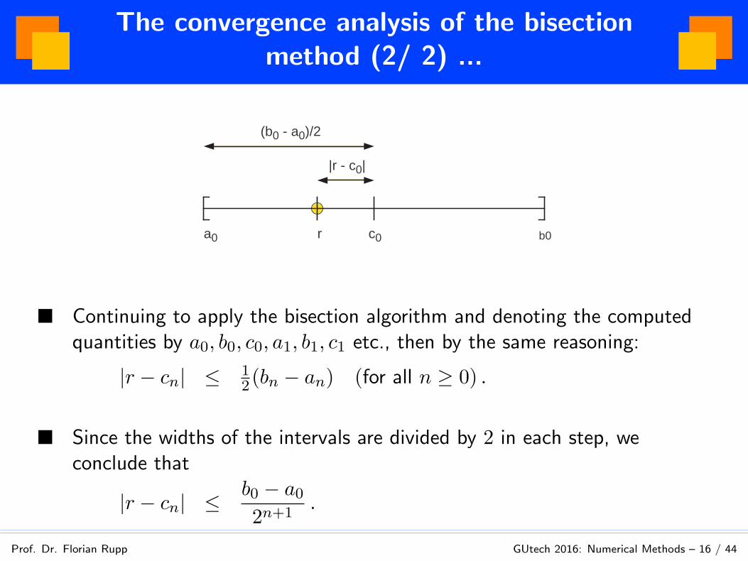
■ The key idea of the regula falsi is to use the point where the secant linebetween f(a) and f(b) intersects the x-axis rather than the midpoint ofeach interval. I.e., the new estimate c for the root is determined as
c = b− f(b)
(
a− b
f(a)− f(b)
)
= a− f(a)
(
b− a
f(b)− f(a)
)
=af(b)− bf(a)
f(b)− f(a).
This still retains the main feature of the bisection method, namely to trapa root in a sequence of intervals of decreasing size.

The key idea of the regula falsi (2/ 4)
Prof. Dr. Florian Rupp GUtech 2016: Numerical Methods – 25 / 44
Illustration of the update mechanism of the regula falsi (initial step):
a
b
f(a) < 0
f(b) > 0
f(c) < 0
c
secant line
The key idea of the regula falsi (3/ 4)
Prof. Dr. Florian Rupp GUtech 2016: Numerical Methods – 26 / 44
Illustration of the update mechanism of the regula falsi (1st step):
a
b
f(a) < 0
f(b) > 0
f(c) < 0
c
secant line

The key idea of the regula falsi (4/ 4)
Prof. Dr. Florian Rupp GUtech 2016: Numerical Methods – 27 / 44
Illustration of the update mechanism of the regula falsi (2nd step):
a
b
f(a) < 0
f(b) > 0secant line

Does the regula falsi really increase thebisection method’s speed?
Prof. Dr. Florian Rupp GUtech 2016: Numerical Methods – 28 / 44
■ For some functions, the regula falsi may repeatedly select the sameendpoint (like in our example), and the whole process may degrade tolinear convergence.
■ This is always the case if f(x) is convex or concave in a subdivisioninterval [ak, bk], i.e., if f
′′(x) has the same sign in that whole interval.Here, one of the interval boundaries than stays the same for allconsecutive times, whereas the other converges linearly towards the root.
Theorem (Super-Linear Convergence Using the Regula Falsi)
The bisection method with a variant of the regula falsi has super-linear conver-gence towards the root, as long as f is not strictly convex or strictly concave inone of the subdivision intervals (i.e., as long as it is provided that the secondderivative has a sign change in any subdivision interval). We will see that later.
Modification of the regula falsi (1/ 3)
Prof. Dr. Florian Rupp GUtech 2016: Numerical Methods – 29 / 44
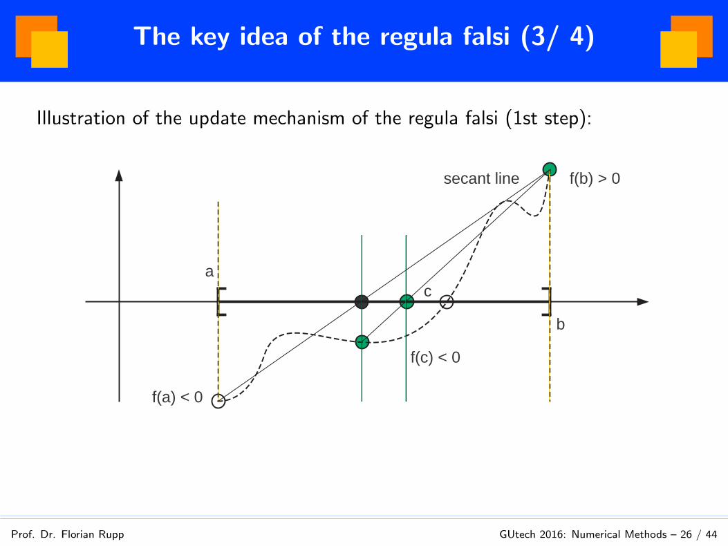
For example, when the same endpoint is to be retained twice, a modifiedregula falsi may use
cn :=
anf(bn)− bnf(an)
f(bn)− f(an)if f(an)f(bn) < 0
2anf(bn)− bnf(an)
2f(bn)− f(an)if f(an)f(bn) > 0
So rather than selecting points on the same side of the root as the normal
regula falsi this modified method changes the slope of the straight line. This
produces estimates for the root that are closer to it than those obtained by
the normal regula falsi method.

Modification of the regula falsi (2/ 3)
Prof. Dr. Florian Rupp GUtech 2016: Numerical Methods – 30 / 44
Illustration of the modified regula falsi (normal initial step):
a
b
f(a) < 0
f(b) > 0
f(c) < 0
c
secant line

Modification of the regula falsi (3/ 3)
Prof. Dr. Florian Rupp GUtech 2016: Numerical Methods – 31 / 44
Illustration of the modified regula falsi (modified 1st step):
a
b
f(a) < 0
f(b) > 0
c
secant line
0.5 f(b)

Newton’s method

The key idea of Newton’s method (1/ 2)
Prof. Dr. Florian Rupp GUtech 2016: Numerical Methods – 33 / 44
■ In Newton’s method, it is assumed that the function f is differentiable.This implies that the graph of f has a definite slope at each point andhence an unique tangent line.
■ At a certain point (x0, f(x0)) on the graph of f the tangent is a rathergood approximation of the function in the vicinity of that point.Analytically, this means that the linear function
l(x) = f ′(x0)(x− x0) + f(x0)
is close to the given function f near x0; at x0 the two functions f and lagree.
■ In Newton’s method, we take the zero of the linear approximation l as anapproximation of the root of the non-linear function f . This zero is easilyfound:
x1 = x0 −f(x0)
f ′(x0).

The key idea of Newton’s method (2/ 2)
Prof. Dr. Florian Rupp GUtech 2016: Numerical Methods – 34 / 44
■ Thus, starting at a point x0, we pass to a new point x1 obtained from thepreceding formula.
■ Naturally, this procedure can be repeated (iterated) to produce asequence of points:
x2 = x1 −f(x1)
f ′(x1), x3 = x2 −
f(x2)
f ′(x2), and so on .
■ Under favorable conditions, the sequence of points approaches a root of f .
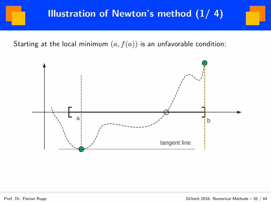
Illustration of Newton’s method (1/ 4)
Prof. Dr. Florian Rupp GUtech 2016: Numerical Methods – 35 / 44
Starting at the local minimum (a, f(a)) is an unfavorable condition:
a b
tangent line

Illustration of Newton’s method (2/ 4)
Prof. Dr. Florian Rupp GUtech 2016: Numerical Methods – 36 / 44
Perturbing the initial point gives a better starting step towards the root, ...
a b
tangent line
x0 x1
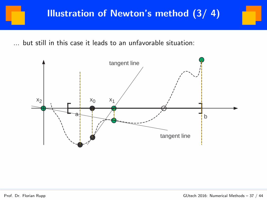
Illustration of Newton’s method (3/ 4)
Prof. Dr. Florian Rupp GUtech 2016: Numerical Methods – 37 / 44
... but still in this case it leads to an unfavorable situation:
a b
tangent line
x0 x1
tangent line
x2
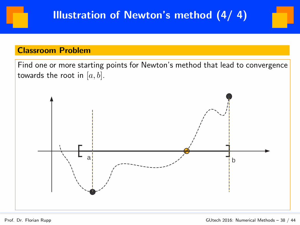
Illustration of Newton’s method (4/ 4)
Prof. Dr. Florian Rupp GUtech 2016: Numerical Methods – 38 / 44
Classroom Problem
Find one or more starting points for Newton’s method that lead to convergencetowards the root in [a, b].
a b

Illustration of Newton’s method withanother function
Prof. Dr. Florian Rupp GUtech 2016: Numerical Methods – 39 / 44
Classroom Problem
Apply Newton’s method graphically to the function f(x) = x3 − x + 1 withx0 = 1.
Compute the Newton iteration points x1 and x2 analytically, using the Newtonupdate formula
xn+1 = xn −f(xn)
f ′(xn).

Summary & Outlook
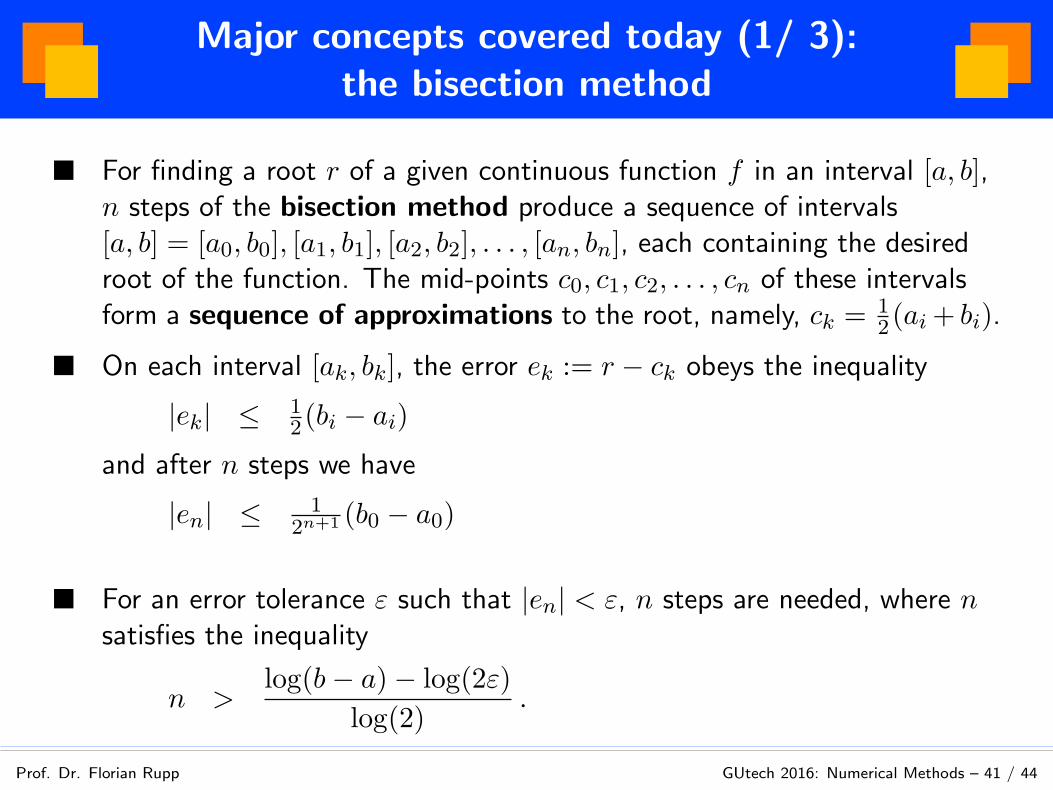
Major concepts covered today (1/ 3):the bisection method
Prof. Dr. Florian Rupp GUtech 2016: Numerical Methods – 41 / 44
■ For finding a root r of a given continuous function f in an interval [a, b],n steps of the bisection method produce a sequence of intervals[a, b] = [a0, b0], [a1, b1], [a2, b2], . . . , [an, bn], each containing the desiredroot of the function. The mid-points c0, c1, c2, . . . , cn of these intervalsform a sequence of approximations to the root, namely, ck = 1
2(ai+ bi).
■ On each interval [ak, bk], the error ek := r − ck obeys the inequality
|ek| ≤ 12(bi − ai)
and after n steps we have
|en| ≤ 12n+1 (b0 − a0)
■ For an error tolerance ε such that |en| < ε, n steps are needed, where nsatisfies the inequality
n >log(b− a)− log(2ε)
log(2).

Major concepts covered today (2/ 3):regula falsi
Prof. Dr. Florian Rupp GUtech 2016: Numerical Methods – 42 / 44
■ For the k-th step of the regula falsi over the interval [ak, bk], let
ck :=akf(bk)− bkf(ak)
f(bk)− f(ak).
If f(ak)f(ck) > 0, set ak+1 = ck and bk+1 = bk; otherwise, set ak+1 = akand bk+1 = ck.
■ A modification of the regula fasli can be obtained by changing the slopeof the secant, e.g., via using the update formula
ck :=
akf(bk)− bkf(ak)
f(bk)− f(ak)if f(ak)f(bk) < 0
2akf(bk)− bkf(ak)
2f(bk)− f(ak)if f(ak)f(bk) > 0

Major concepts covered today (3/ 3):Newton’s method
Prof. Dr. Florian Rupp GUtech 2016: Numerical Methods – 43 / 44
■ For finding a root of a continuously differentiable function f , Newton’smethod is given by
xn+1 = xn −f(xn)
f ′(xn)(n ≥ 0) .
It requires a given initial value x0 and two function evaluation (for f andf ′) at each step.

Preparation for the next lecture
Prof. Dr. Florian Rupp GUtech 2016: Numerical Methods – 44 / 44
Please, prepare these short exercises for the next lecture:
1. Page 123, exercise 1Find where the graphs of y = 3x and y = exp(x) intersect by finding solu-
tions of exp(x)− 3x = 0 correct to four decimal digits with the bisection
method.
2. Page 123, exercise 1 (reformulated)Find where the graphs of y = 3x and y = exp(x) intersect by finding
solutions of exp(x)− 3x = 0 correct to four decimal digits with Newton’s
method.
3. Computer exerciseWrite a MATLAB program that solves exp(x) − 3x = 0 with Newton’s
method and plot the resulting error over the number of iterations (conver-
gence plot).