Determining soil engineering parameters from CPT · PDF fileCorrelations to the following...
33
Determining soil engineering parameters from CPT data
Transcript of Determining soil engineering parameters from CPT · PDF fileCorrelations to the following...
Determining soil engineering
parameters from CPT data

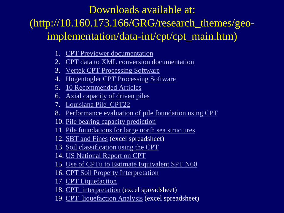
Downloads available at:
(http://10.160.173.166/GRG/research_themes/geo-
implementation/data-int/cpt/cpt_main.htm)
1. CPT Previewer documentation
2. CPT data to XML conversion documentation
3. Vertek CPT Processing Software
4. Hogentogler CPT Processing Software
5. 10 Recommended Articles
6. Axial capacity of driven piles
7. Louisiana Pile_CPT22
8. Performance evaluation of pile foundation using CPT
10. Pile bearing capacity prediction
11. Pile foundations for large north sea structures
12. SBT and Fines (excel spreadsheet)
13. Soil classification using the CPT
14. US National Report on CPT
15. Use of CPTu to Estimate Equivalent SPT N60
16. CPT Soil Property Interpretation
17. CPT Liquefaction
18. CPT_interpretation (excel spreadsheet)
19. CPT_liquefaction Analysis (excel spreadsheet)
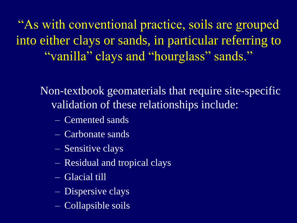
“As with conventional practice, soils are grouped
into either clays or sands, in particular referring to
“vanilla” clays and “hourglass” sands.”
Non-textbook geomaterials that require site-specific
validation of these relationships include:
– Cemented sands
– Carbonate sands
– Sensitive clays
– Residual and tropical clays
– Glacial till
– Dispersive clays
– Collapsible soils
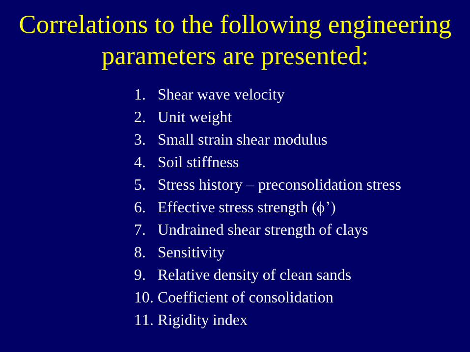
Correlations to the following engineering
parameters are presented:
1. Shear wave velocity
2. Unit weight
3. Small strain shear modulus
4. Soil stiffness
5. Stress history – preconsolidation stress
6. Effective stress strength (f’)
7. Undrained shear strength of clays
8. Sensitivity
9. Relative density of clean sands
10. Coefficient of consolidation
11. Rigidity index
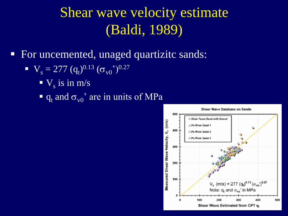
Shear wave velocity estimate
(Baldi, 1989)
For uncemented, unaged quartizitc sands:
Vs = 277 (qt)0.13 (sv0’)
0.27
Vs is in m/s
qt and sv0’ are in units of MPa
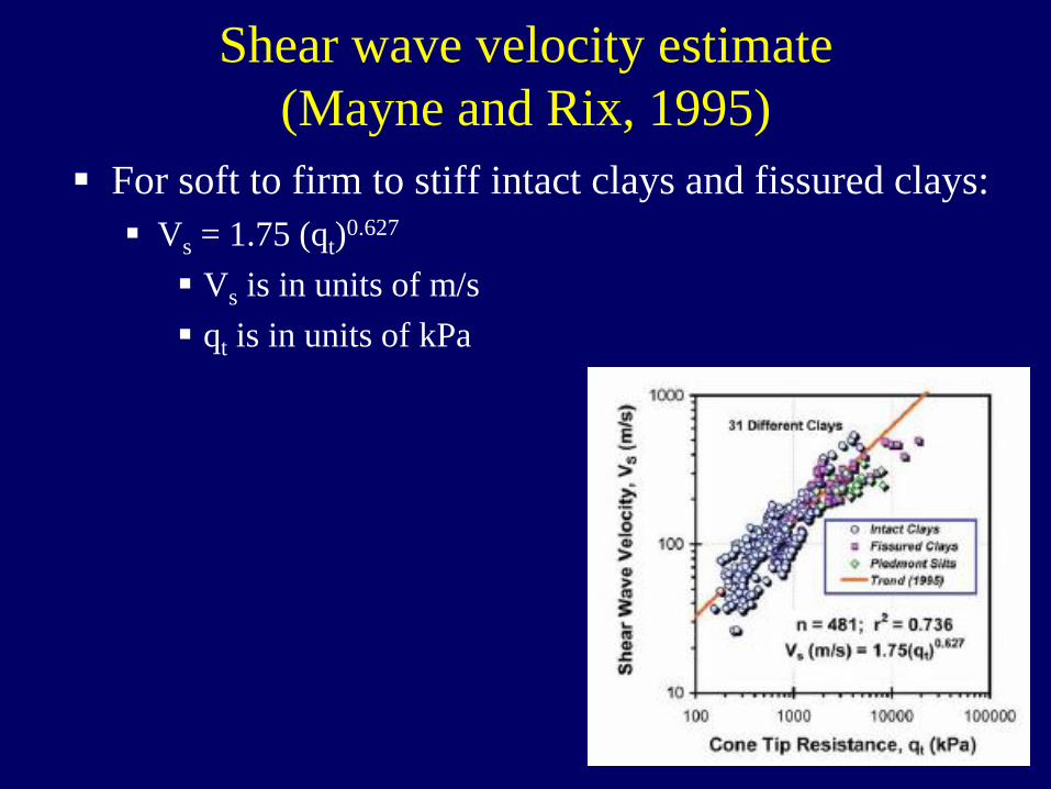
Shear wave velocity estimate
(Mayne and Rix, 1995)
For soft to firm to stiff intact clays and fissured clays:
Vs = 1.75 (qt)0.627
Vs is in units of m/s
qt is in units of kPa
Shear wave velocity estimation methods
(Hegazy and Mayne, 1995)
For all soil types:
Vs = ((10.1) (log qt) – 11.4))1.67 ((fs/qt) (100))0.3
Vs is in m/s
qt and fs are in units of kPa
For all saturated soils:
Vs = (118.8) (log fs) + 18.5
Vs is in units of m/s
fs is in units of kPa
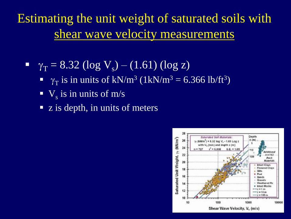
Estimating the unit weight of saturated soils with
shear wave velocity measurements
gT = 8.32 (log Vs) – (1.61) (log z)
gT is in units of kN/m3 (1kN/m3 = 6.366 lb/ft3)
Vs is in units of m/s
z is depth, in units of meters
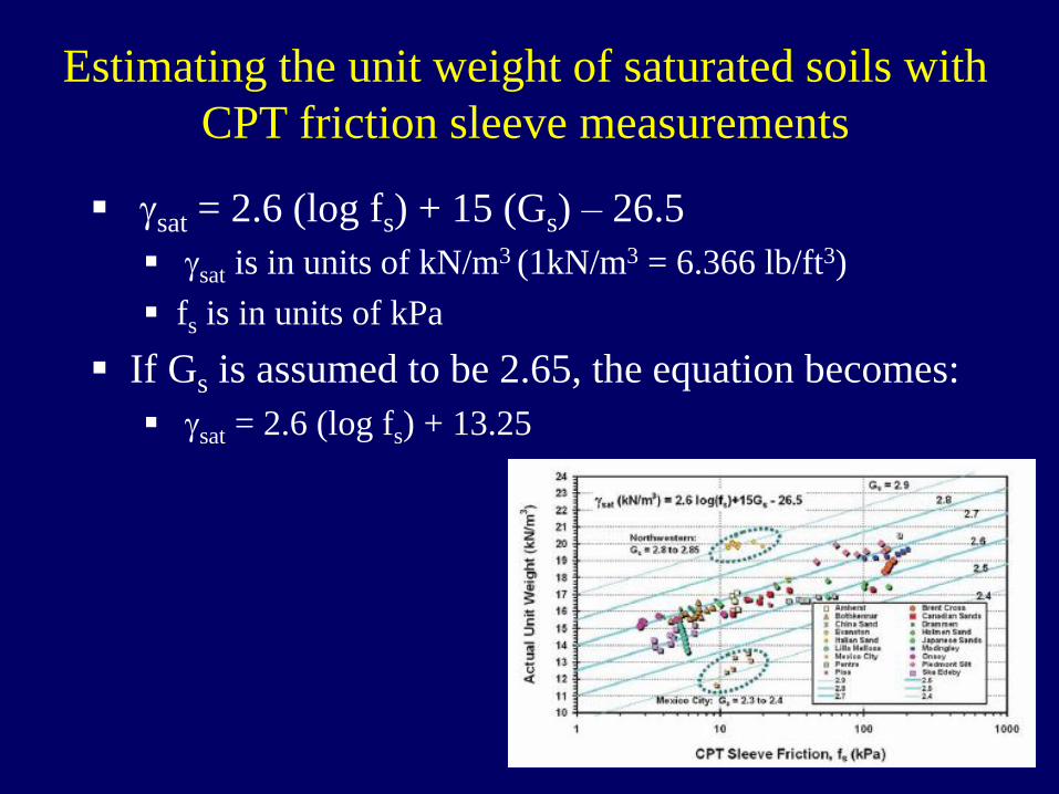
Estimating the unit weight of saturated soils with
CPT friction sleeve measurements
gsat = 2.6 (log fs) + 15 (Gs) – 26.5
gsat is in units of kN/m3 (1kN/m3 = 6.366 lb/ft3)
fs is in units of kPa
If Gs is assumed to be 2.65, the equation becomes:
gsat = 2.6 (log fs) + 13.25
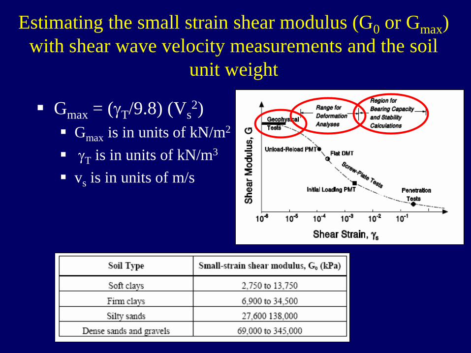
Estimating the small strain shear modulus (G0 or Gmax)
with shear wave velocity measurements and the soil
unit weight
Gmax = (gT/9.8) (Vs2)
Gmax is in units of kN/m2
gT is in units of kN/m3
vs is in units of m/s
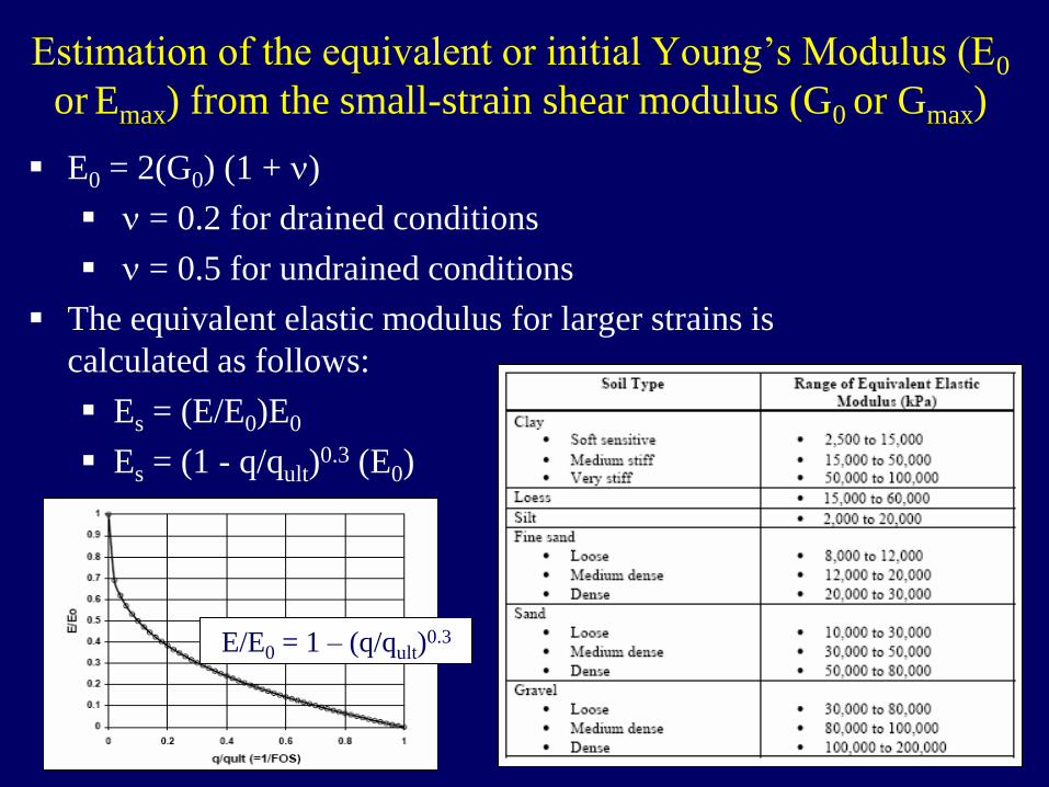
Estimation of the equivalent or initial Young’s Modulus (E0
or Emax) from the small-strain shear modulus (G0 or Gmax)
E0 = 2(G0) (1 + n)
n = 0.2 for drained conditions
n = 0.5 for undrained conditions
The equivalent elastic modulus for larger strains is
calculated as follows:
Es = (E/E0)E0
Es = (1 - q/qult)0.3 (E0)
E/E0 = 1 – (q/qult)0.3
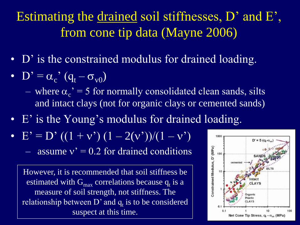
Estimating the drained soil stiffnesses, D’ and E’,
from cone tip data (Mayne 2006)
• D’ is the constrained modulus for drained loading.
• D’ = ac’ (qt – sv0)
– where ac’ = 5 for normally consolidated clean sands, silts
and intact clays (not for organic clays or cemented sands)
• E’ is the Young’s modulus for drained loading.
• E’ = D’ ((1 + n’) (1 – 2(n’))/(1 – n’)
– assume n’ = 0.2 for drained conditions
However, it is recommended that soil stiffness be
estimated with Gmax correlations because qt is a
measure of soil strength, not stiffness. The
relationship between D’ and qt is to be considered
suspect at this time.
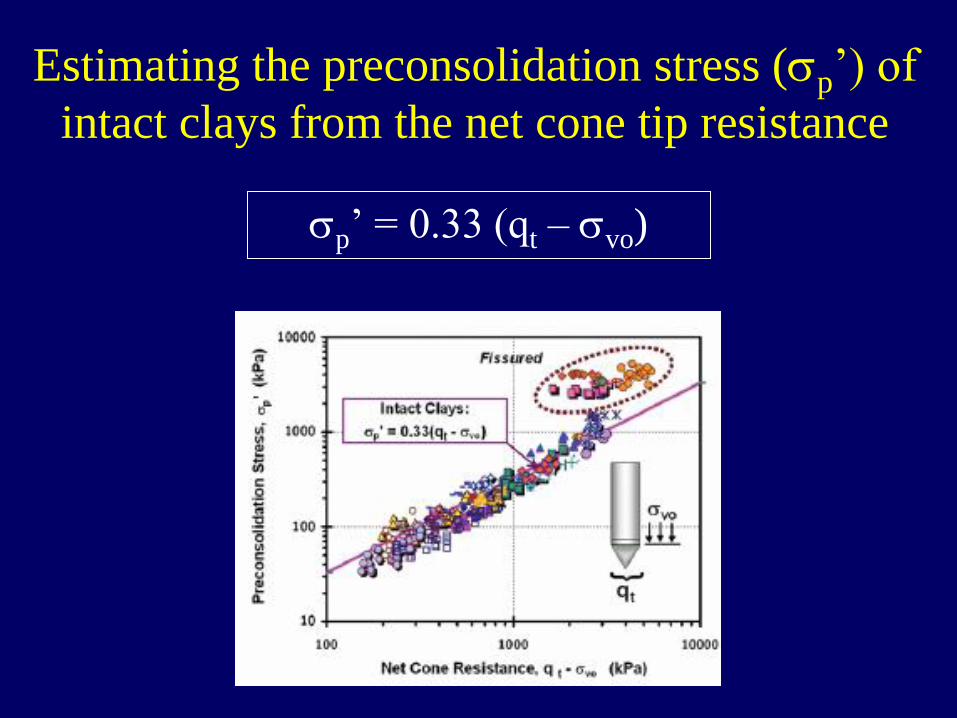
Estimating the preconsolidation stress (sp’) of
intact clays from the net cone tip resistance
sp’ = 0.33 (qt – svo)
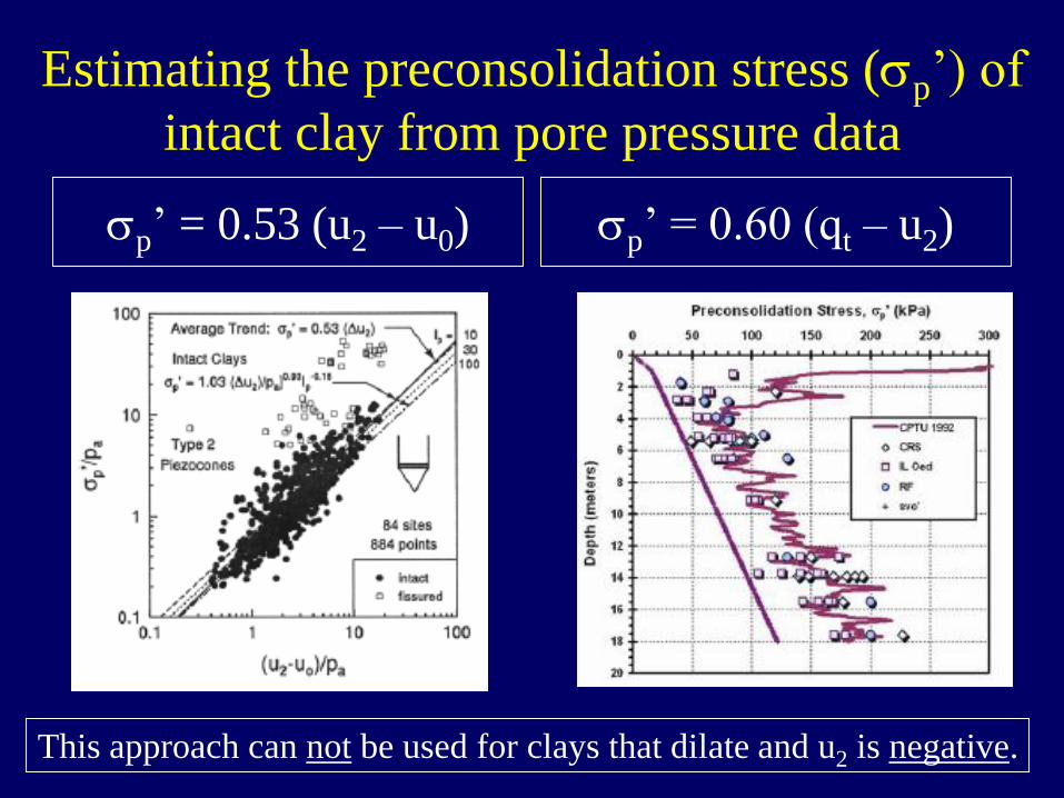
Estimating the preconsolidation stress (sp’) of
intact clay from pore pressure data
sp’ = 0.53 (u2 – u0) sp’ = 0.60 (qt – u2)
This approach can not be used for clays that dilate and u2 is negative.
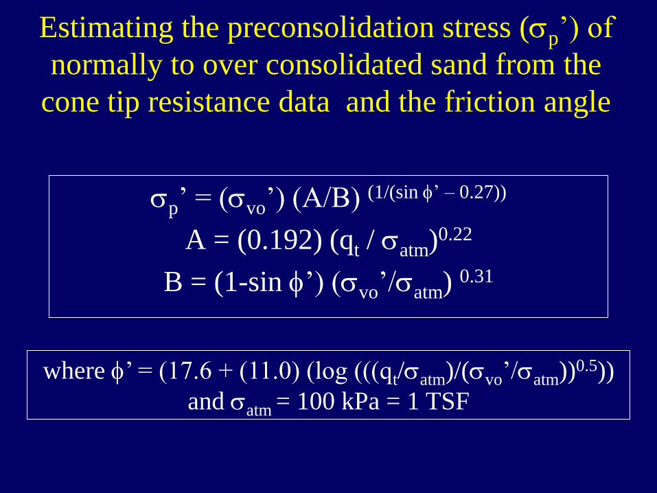
Estimating the preconsolidation stress (sp’) of
normally to over consolidated sand from the
cone tip resistance data and the friction angle
sp’ = (svo’) (A/B) (1/(sin f’ – 0.27))
A = (0.192) (qt / satm)0.22
B = (1-sin f’) (svo’/satm) 0.31
where f’ = (17.6 + (11.0) (log (((qt/satm)/(svo’/satm))0.5))
and satm = 100 kPa = 1 TSF
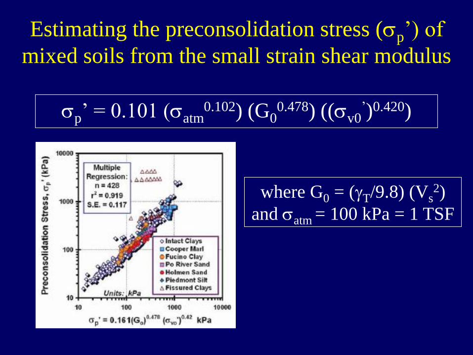
Estimating the preconsolidation stress (sp’) of
mixed soils from the small strain shear modulus
sp’ = 0.101 (satm0.102) (G0
0.478) ((sv0’)0.420)
where G0 = (gT/9.8) (Vs2)
and satm = 100 kPa = 1 TSF
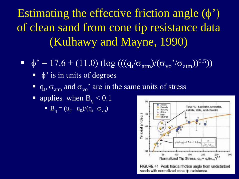
Estimating the effective friction angle (f’)
of clean sand from cone tip resistance data
(Kulhawy and Mayne, 1990)
f’ = 17.6 + (11.0) (log (((qt/satm)/(svo’/satm))0.5))
f’ is in units of degrees
qt, satm and svo’ are in the same units of stress
applies when Bq < 0.1
Bq = (u2 –u0)/(qt –svo)
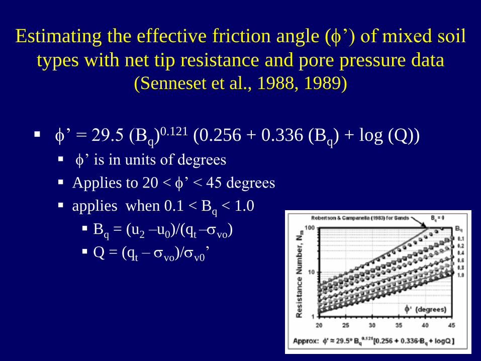
Estimating the effective friction angle (f’) of mixed soil
types with net tip resistance and pore pressure data(Senneset et al., 1988, 1989)
f’ = 29.5 (Bq)0.121 (0.256 + 0.336 (Bq) + log (Q))
f’ is in units of degrees
Applies to 20 < f’ < 45 degrees
applies when 0.1 < Bq < 1.0
Bq = (u2 –u0)/(qt –svo)
Q = (qt – svo)/sv0’
Estimating the undrained shear strength (su) of
clays from the preconsolidation stress (sp’)
For OCR < 2
Based on vane shear tests and back analysis from
failures for embankments, footings and excavations.
Fissured clays can exhibit su values 50% of the su of
non-fissured clays. Fissured clays can be identified
by the negative pore pressures during penetration.
su = 0.22 (sp’)
Estimating the undrained shear strength (su) of
clays from correlation with local experience
su = (qt – sv0)/Nkt
• Nkt is determined from
local experience.
• Nkt is correlated to specific
lab or field undrained shear
strength test methods.
Estimating the sensitivity of soft clays
For low OC clays, OCR < 2
The friction sleeve measurement is regarded as an
indication of the remolded shear strength.
fs = sur
Combining this formula with two of the
previously presented relationships:
sp’ = 0.33 (qt – svo)
su = 0.22 (sp’)
St = 0.073 (qt – svo)/fs
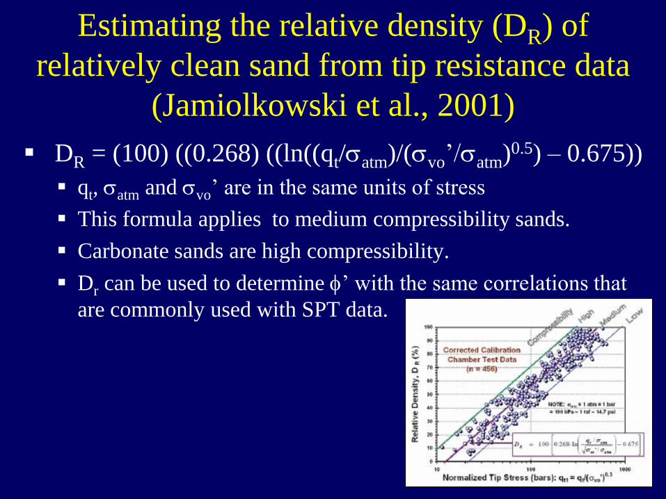
Estimating the relative density (DR) of
relatively clean sand from tip resistance data
(Jamiolkowski et al., 2001)
DR = (100) ((0.268) ((ln((qt/satm)/(svo’/satm)0.5) – 0.675))
qt, satm and svo’ are in the same units of stress
This formula applies to medium compressibility sands.
Carbonate sands are high compressibility.
Dr can be used to determine f’ with the same correlations that
are commonly used with SPT data.
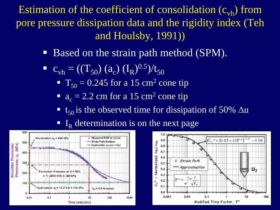
Estimation of the coefficient of consolidation (cvh) from
pore pressure dissipation data and the rigidity index (Teh
and Houlsby, 1991))
Based on the strain path method (SPM).
cvh = ((T50) (ac) (IR)0.5)/t50
T50 = 0.245 for a 15 cm2 cone tip
ac = 2.2 cm for a 15 cm2 cone tip
t50 is the observed time for dissipation of 50% Du
IR determination is on the next page
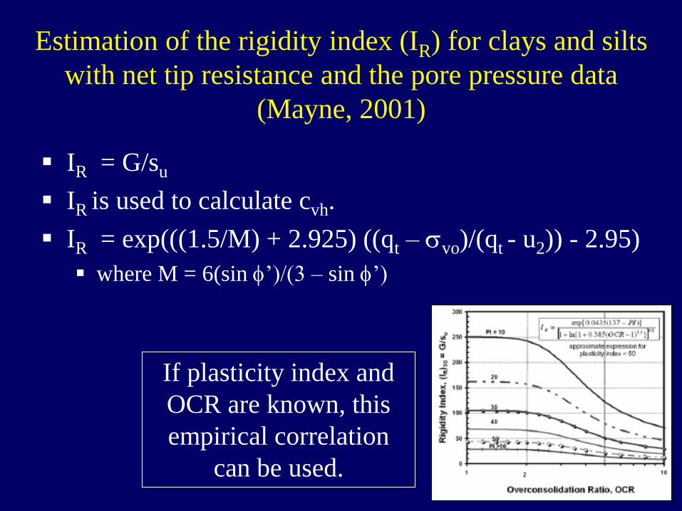
Estimation of the rigidity index (IR) for clays and silts
with net tip resistance and the pore pressure data
(Mayne, 2001)
IR = G/su
IR is used to calculate cvh.
IR = exp(((1.5/M) + 2.925) ((qt – svo)/(qt - u2)) - 2.95)
where M = 6(sin f’)/(3 – sin f’)
If plasticity index and
OCR are known, this
empirical correlation
can be used.
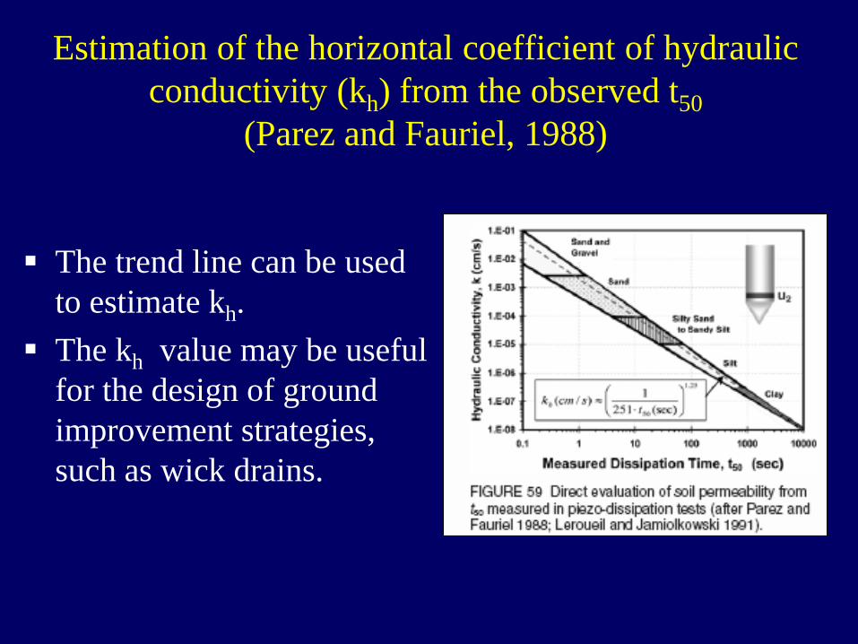
Estimation of the horizontal coefficient of hydraulic
conductivity (kh) from the observed t50
(Parez and Fauriel, 1988)
The trend line can be used
to estimate kh.
The kh value may be useful
for the design of ground
improvement strategies,
such as wick drains.
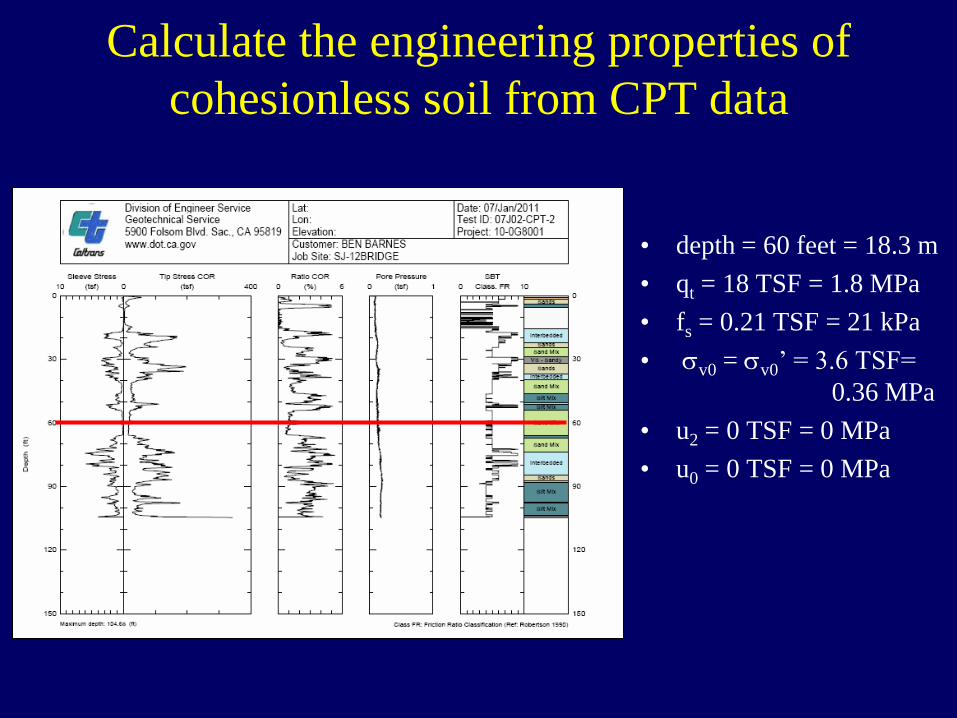
Calculate the engineering properties of
cohesionless soil from CPT data
• depth = 60 feet = 18.3 m
• qt = 18 TSF = 1.8 MPa
• fs = 0.21 TSF = 21 kPa
• sv0 = sv0’ = 3.6 TSF=
0.36 MPa
• u2 = 0 TSF = 0 MPa
• u0 = 0 TSF = 0 MPa
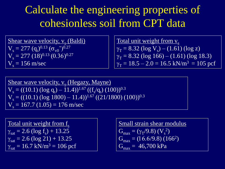
Total unit weight from vs
gT = 8.32 (log Vs) – (1.61) (log z)
gT = 8.32 (log 166) – (1.61) (log 18.3)
gT = 18.5 – 2.0 = 16.5 kN/m3 = 105 pcf
Shear wave velocity, vs (Baldi)
Vs = 277 (qt)0.13 (sv0’)
0.27
Vs = 277 (18)0.13 (0.36)0.27
Vs = 156 m/sec
Small strain shear modulus
Gmax = (gT/9.8) (Vs2)
Gmax = (16.6/9.8) (1662)
Gmax = 46,700 kPa
Shear wave velocity, vs (Hegazy, Mayne)
Vs = ((10.1) (log qt) – 11.4))1.67 ((fs/qt) (100))0.3
Vs = ((10.1) (log 1800) – 11.4))1.67 ((21/1800) (100))0.3
Vs = 167.7 (1.05) = 176 m/sec
Total unit weight from fs
gsat = 2.6 (log fs) + 13.25
gsat = 2.6 (log 21) + 13.25
gsat = 16.7 kN/m3 = 106 pcf
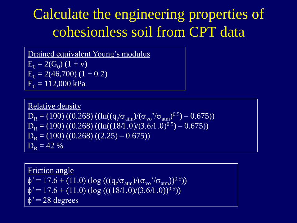
Calculate the engineering properties of
cohesionless soil from CPT data
Calculate the engineering properties of
cohesionless soil from CPT data
Friction angle
f’ = 17.6 + (11.0) (log (((qt/satm)/(svo’/satm))0.5))
f’ = 17.6 + (11.0) (log (((18/1.0)/(3.6/1.0))0.5))
f’ = 28 degrees
Relative density
DR = (100) ((0.268) ((ln((qt/satm)/(svo’/satm)0.5) – 0.675))
DR = (100) ((0.268) ((ln((18/1.0)/(3.6/1.0)0.5) – 0.675))
DR = (100) ((0.268) ((2.25) – 0.675))
DR = 42 %
Drained equivalent Young’s modulus
E0 = 2(G0) (1 + n)
E0 = 2(46,700) (1 + 0.2)
E0 = 112,000 kPa
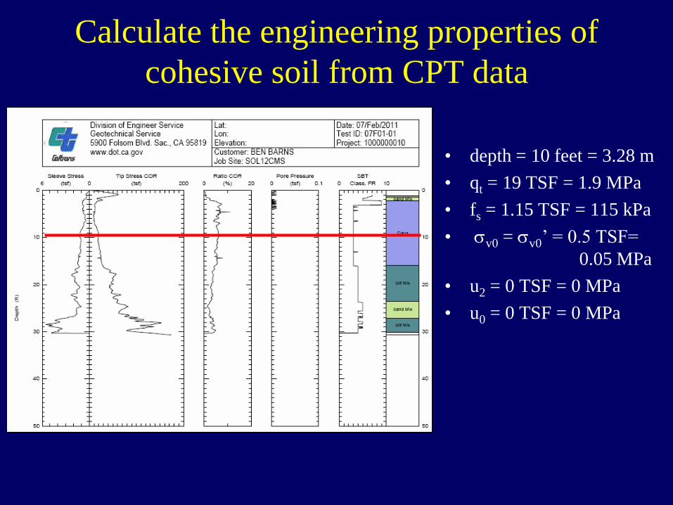
Calculate the engineering properties of
cohesive soil from CPT data
• depth = 10 feet = 3.28 m
• qt = 19 TSF = 1.9 MPa
• fs = 1.15 TSF = 115 kPa
• sv0 = sv0’ = 0.5 TSF=
0.05 MPa
• u2 = 0 TSF = 0 MPa
• u0 = 0 TSF = 0 MPa
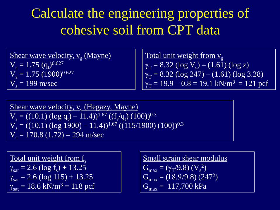
Calculate the engineering properties of
cohesive soil from CPT data
Total unit weight from vs
gT = 8.32 (log Vs) – (1.61) (log z)
gT = 8.32 (log 247) – (1.61) (log 3.28)
gT = 19.9 – 0.8 = 19.1 kN/m3 = 121 pcf
Shear wave velocity, vs (Mayne)
Vs = 1.75 (qt)0.627
Vs = 1.75 (1900)0.627
Vs = 199 m/sec
Small strain shear modulus
Gmax = (gT/9.8) (Vs2)
Gmax = (18.9/9.8) (2472)
Gmax = 117,700 kPa
Shear wave velocity, vs (Hegazy, Mayne)
Vs = ((10.1) (log qt) – 11.4))1.67 ((fs/qt) (100))0.3
Vs = ((10.1) (log 1900) – 11.4))1.67 ((115/1900) (100))0.3
Vs = 170.8 (1.72) = 294 m/sec
Total unit weight from fs
gsat = 2.6 (log fs) + 13.25
gsat = 2.6 (log 115) + 13.25
gsat = 18.6 kN/m3 = 118 pcf
Calculate the engineering properties of
cohesive soil from CPT data
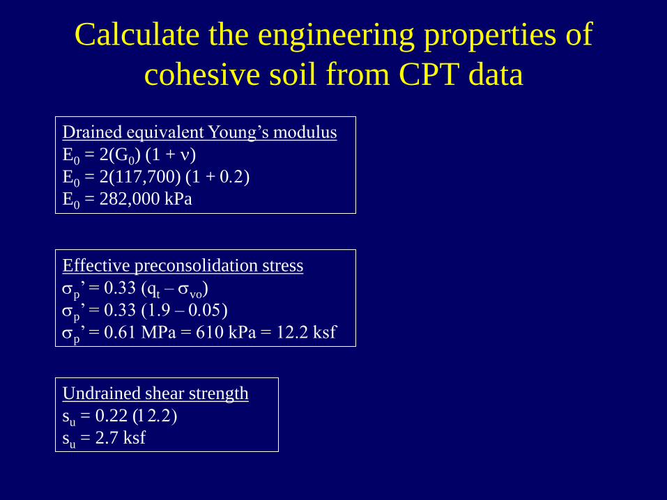
Undrained shear strength
su = 0.22 (12.2)
su = 2.7 ksf
Effective preconsolidation stress
sp’ = 0.33 (qt – svo)
sp’ = 0.33 (1.9 – 0.05)
sp’ = 0.61 MPa = 610 kPa = 12.2 ksf
Drained equivalent Young’s modulus
E0 = 2(G0) (1 + n)
E0 = 2(117,700) (1 + 0.2)
E0 = 282,000 kPa

Questions?