Determining Factors that Affect Survival of Moose in Central British Columbia

Matthew A. Mumma and Michael P. Gillingham

Technical Report to the Habitat Conservation Trust Foundation for Grant Agreement CAT19-0-522

(1 April 2017 through 31 March 2019)

i

Executive Summary Over the last decade moose (Alces alces) populations in parts of interior British Columbia have declined by 50–70%; other populations are stable or increasing (Kuzyk 2016). Declines have coincided with mountain pine beetle (MPB) (Dendroctonus ponderosae) outbreaks and related salvage harvesting and road building — landscape changes that could influence the distribution and abundance of moose, hunters, and predators. In 2013, the Ministry of Forests, Lands, Natural Resource Operations and Rural Development (FLNRORD) initiated a five-year provincially coordinated research project (Kuzyk and Heard 2014). The FLNRORD cow-survival study was designed to test the landscape-change hypothesis. The expectation was that moose survival would increase when: cutblocks regenerate to the point where vegetation obstructs the view of predators and hunters; resource roads created for logging are deactivated; and moose become more uniformly dispersed on the landscape (Kuzyk and Heard 2014). We completed a comprehensive analysis of cow moose survival evaluating FLNRORD’s ‘landscape-change’ hypothesis and examining factors contributing to mortality for cow moose across six study areas (Big Creek, Bonaparte, Entiako, John Prince Research Forest [JPRF], Prince George South, and West Parsnip) in interior BC. Analyses examined similarities and differences in survival among study areas and focused on linking disturbances to moose survival and key management levers identified in the provincial framework for moose management (BC FLNRO 2015) and echoed in the Gorley (2016) report. Those potential actions (or levers) included: hunting regulations, First Nations harvest, predator management, access management, habitat enhancement and protection, and environmental assessment and mitigation identified in the provincial framework for moose management (BC FLNRO 2015). During the winters of 2012–2018, 456 cow moose were fitted with GPS radio-collars. As of July 31, 2018, 230 of these collars remained active, 105 were no longer transmitting locations, and 121 collared moose were confirmed dead. In conjunction with provincial biologists, consultants (for West Parsnip), and veterinarians, we determined ultimate causes of death using observations from mortality locations and indices of moose condition at time of death. The most frequent causes of death were wolf (Canis lupus) predation (n = 51), apparent starvation (n = 17), and human harvest (n = 16). We compared causes of death across study areas and generated study area-specific Kaplan-Meier survival curves (Kaplan and Meier 1958). Wolf predation was the only cause of death observed in every study area and predominant cause of death in all but one study area. Human harvest was the predominant cause of death in the Bonaparte study area and was observed in three of the other study areas. Apparent starvation was observed in five of the six study areas. Yearly survival estimates for adult cow moose ranged from 81.10–92.45% with a mean value of 86.80% across study areas. We modelled the influence of disturbances and weather on risk from the leading causes of death using the Anderson-Gill formulation (Anderson and Gill 1982) of the Cox proportional hazards model (Cox 1972) under a competing-risks framework (Fine and Gray 1999). To preserve statistical power, we combined causes of death into four categories: wolf predation, human harvest, apparent

ii

starvation, and other causes (several minor causes and unknown causes of death). We anticipated that the effects on covariates on each category of risk might depend on their spatial and temporal scale. For example, we hypothesized that being in a cutblock would increase the risk of human harvest for a given day or week, but that the risk of apparent starvation would be more likely related to the use of cutblocks by an individual moose over the previous few months or year. We, therefore, built models to identify the most informative scale for each disturbance covariate. We then built candidate models based on hypothesized mechanisms linking disturbances to wolf predation, hunting, and apparent starvation and selected the best-supported models using an information-theoretic approach (Burnham and Anderson 2002). Our best-supported model included covariates for road density and the proportion of new cutblocks (1–8 years) estimated within 200-m and 400-m radii, respectively, around each moose location. The strongest responses relating roads and new cutblocks to the three leading causes of death (wolf predation, human harvest, and apparent starvation) included the following:

• moose were more likely to be killed by wolves if they were in areas with lower road densities over the previous 365 days;

• moose were more likely to be harvested by human hunters if they were in areas with higher road densities on a given day and higher proportions of new cutblocks over the previous seven days; and

• moose were more likely to die from apparent starvation if they were in areas with higher road densities over the previous 365 days and higher proportions of new cutblocks over the previous 180 days.

To tease apart potential seasonal relationships between disturbance and apparent starvation, we examined individuals that had survived >1 year post-collaring and compared the previous year’s seasonal habitat use between individuals that died from apparent starvation versus the remaining individuals using logistic regression. We built candidate models that tested the influence of changes in forage and a reduction in canopy cover as it related to the costs of thermoregulation (thermal stress) and the costs of movement in deep or dense snow (snow interception). Our snow-interception model was best supported, and suggested that moose that used areas in winter with high proportions of new cutblocks, new burns, and pine were more likely to die from apparent starvation. Our thermal-stress model was the second best-supported model and included the same covariates as the snow-interception model, but estimated during the entire non-growing period (i.e., fall and winter). Our analyses of cow moose survival in BC revealed several key insights that will contribute to moose management moving forward. Although the lower range of yearly survival observed for some study areas was lower than would be anticipated for a healthy moose population, cow moose survival alone does not explain the declines observed for moose abundance in interior BC. This suggests that under current conditions calf recruitment might be more limiting than cow survival. Wolves were the primary cause of death for moose in central BC, but the data did not suggest that wolf predation on cow moose was higher near disturbances. In contrast, mortality from hunting and apparent starvation was increased as a result of roads and new cutblocks. Given the limited cow

iii

moose hunting permitted in these study areas, we did not expect to observe high amounts of licensed hunting (n = 1), but the number unlicensed kills (n = 15) was higher than anticipated. The number of apparent starvations was also greater than anticipated and likely indicates an overall decrease in moose health and condition that might be contributing to lower calf recruitment. Decreased body condition in cow moose might lower pregnancy rates and lead to weaker calves with higher rates of mortality from predation or other causes. The direct effects, however, of disturbances on the hunting success for wolves, bears (Ursus spp.), or cougars (Puma concolor) on calves might also lead to lower calf survival. Notably, bear predation on cow moose was observed during the spring, which is when bear predation on calves is also expected to be greatest, thus suggesting that bears might be targeting and killing calves during this time. Future research should focus on the survival of early born calves and continue until they are recruited into the breeding population. Consistent with the Habitat Conservation Trust Foundation’s vision, moose and their habitat should be of value to all British Columbians and management actions (Gorley 2016) should be supported by existing data. Given the low number of moose harvested by licensed hunters, a reduction in cow moose tag allocations is unlikely to result in a significant change to moose population growth. Additional efforts, however, should go toward identifying the source of unlicensed harvest, particularly in the Bonaparte, Big Creek, and JPRF study areas. Although predation was not higher near disturbances, wolf predation was the primary cause of death for cow moose. Further, bear predation on cows and presumably calves during the calving season should not be overlooked as a potentially important source of mortality. Predator management might result in higher moose survival leading to higher abundance, but might further exacerbate decreases in cow moose body condition if forage is limiting and also would need be balanced against financial and societal costs. The data suggested that areas with high road densities increased hunter kills and apparent starvations, but might decrease wolf predation; thus, the cumulative effects of deactivating or restoring roads on cow moose survival is uncertain. Given the avoidance of new cutblocks and the increase in hunter kills and apparent starvations in areas with new cutblocks, restoring logging intensity to pre-salvage harvest levels would likely assist in stabilizing moose populations in interior BC.

iv

Table of Contents Executive Summary ................................................................................................................................... i

Table of Contents ..................................................................................................................................... iv

List of Figures ........................................................................................................................................... vi

List of Tables .......................................................................................................................................... viii

Acknowledgments .................................................................................................................................... ix

Introduction ........................................................................................................................................... 10

Background and Rationale ................................................................................................................. 10

Objectives ........................................................................................................................................... 10

Objective 1: Collate, compile, and screen all current and incoming data for use in survival analyses .......................................................................................................................................... 10

Objective 2: Determine if there are important differences among study areas in factors affecting survival that would suggest regional differences in managing moose .......................... 11

Objective 3: Contrast data from collared animals that have survived versus died to test hypotheses linked to moose management objectives .................................................................. 11

Methods ................................................................................................................................................. 12

Study Areas ........................................................................................................................................ 12

Big Creek ........................................................................................................................................ 12

Bonaparte ...................................................................................................................................... 12

Entiako ........................................................................................................................................... 12

John Prince Research Forest .......................................................................................................... 12

Prince George South ...................................................................................................................... 13

West Parsnip .................................................................................................................................. 14

Collaring and Monitoring of Collared Moose..................................................................................... 14

Cow Moose Collaring, Fates, Transmission Rates, and Success Rates .......................................... 14

Screening for Mortalities ............................................................................................................... 14

Mortality Site Investigations and Proximate Cause of Death ........................................................ 15

Determination of Ultimate Cause of Death ................................................................................... 16

Preparation of Data and Spatial layers .............................................................................................. 18

Screening of Location Data ............................................................................................................ 18

Developing Vegetation and Disturbance Layers ............................................................................ 18

Determining Thresholds for Cutblocks .......................................................................................... 18

Refining Burn Layers ...................................................................................................................... 18

Causes of Death and Survival Estimates by Study Area ..................................................................... 21

v

Determining Kaplan-Meier Survival Curves ................................................................................... 21

Estimating Demographic Rates Required to Achieve Population Stability .................................... 21

Modelling Risk with Cox Proportional Hazards Models ..................................................................... 21

Description of Model ..................................................................................................................... 21

Development of Covariates and Candidate Models ...................................................................... 22

Evaluating Seasonal Space Use and Apparent Starvation ................................................................. 23

Covariates and Candidate Models ................................................................................................. 23

Results .................................................................................................................................................... 25

Causes of Mortality ............................................................................................................................ 25

Ultimate Cause of Death ................................................................................................................ 25

Refined Cutblock and Burn Layers ................................................................................................. 29

Causes of Death and Survival Estimates by Study Area ..................................................................... 31

Causes of Death by Study Area ...................................................................................................... 31

Kaplan-Meier Survival Estimates ................................................................................................... 31

Demographic Rates for Population Stability .................................................................................. 33

Cox Proportional Hazard Models of Risk ........................................................................................... 34

Seasonal Space Use and Apparent Starvation ................................................................................... 34

Discussion............................................................................................................................................... 39

Management Implications ..................................................................................................................... 41

Literature Cited ...................................................................................................................................... 43

Appendix 1: Mortality Site Investigation Form used to assess Cause of Mortality for Moose in Central British Columbia .............................................................................................................. 45

vi

List of Figures Figure 1. Map of the six study areas where survival of collared cows was monitored in British

Columbia from 2012–2018. ...................................................................................................... 11

Figure 2. Parameter settings of Excel macros used to identify mortalities via changes in moose movement. ................................................................................................................................ 15

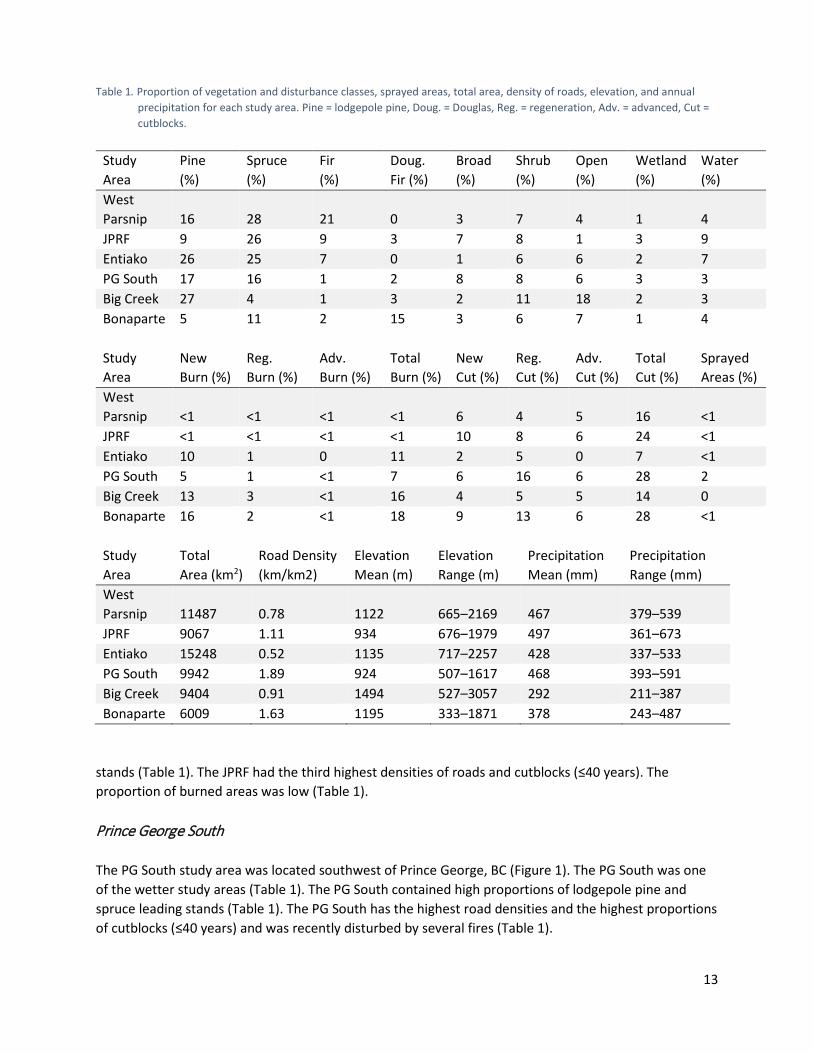
Figure 3. Example of Google Earth output from Excel macro used to identify mortality via changes in moose movement. .................................................................................................. 16

Figure 4. Flow chart used to determine ultimate cause of death for collared moose mortality. ......... 17

Figure 5. Perimeter of Little Bobtail Lake Fire, which burned within the PG South study area in 2015. ......................................................................................................................................... 19

Figure 6. Schematic comparing wavelength (Electromagnetic Spectrum) of pre- and post-burn images (source www.fs.fed.us). ................................................................................................ 20

Figure 7. Estimate of burned and unburned areas within the perimeter of the Little Bobtail Lake fire (2015) as determined via differenced normalized burn ratios using spectral imagery. .... 20

Figure 8. Schematic illustrating the spatial and temporal scales used in survival modelling. Each collared moose location was used to query several underlying covariates (list on left slide of figure) within 200-, 400-, 800-, and 1600-m radii. The values of each covariate at each spatial scale were then back-calculated for 1-, 7-, 14-, 90-, 180-, and 365-day windows. ................................................................................................................................... 22

Figure 9. Schematic of buffered areas around location points (see text) used to assess use by collared cow moose. ................................................................................................................. 25

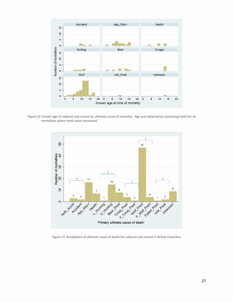
Figure 10. Known age of collared cow moose by ultimate cause of mortality. Age was obtained by sectioning teeth for all mortalities where teeth were recovered. ...................................... 27

Figure 11. Breakdown of ultimate cause of death for collared cow moose in British Columbia. ......... 27

Figure 12. Pooled ultimate causes of death for collared cow moose in British Columbia. ................... 28

Figure 13. Month of the year when the four most common sources of ultimate mortality of collared cow moose occurred. .................................................................................................. 28

Figure 14. Selection ratios (and 95% confidence intervals) as a function of time (years) since cut for moose (right axis) in British Columbia................................................................................. 29

Figure 15. Proportion of areas cut per year and the cumulative proportion of new cutblocks (1–8 years) and regenerating (reg.) cutblocks (9–24 years) in the PG South and Bonaparte study areas. ............................................................................................................................... 30

Figure 16. Area of burn perimeters compares to estimates of the areas burned as identified using differenced normalized burn ratios................................................................................. 31

Figure 17. Ultimate causes of mortality for collared moose in British Columbia by study area. Apparent starvation is displayed by the detached portion of the pie diagrams. ..................... 32

vii

Figure 18. Frequency of licensed and unlicensed hunting by Game Management Unit for collared cow moose in British Columbia................................................................................................. 32

Figure 19. Comparison of Kaplan-Meier survival estimates for all six study areas in which cow moose were collared. The start of collaring differed among study areas with Bonaparte beginning earliest (late winter 2012) and West Parsnip beginning latest (late winter 2017). ........................................................................................................................................ 33

Figure 20. Cox proportional hazard functions for wolf predation, human harvest (hunting), apparent starvation, and other causes for collared cow moose in interior British Columbia. .................................................................................................................................. 35

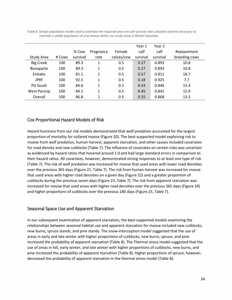
Figure 21. Effect of mean road density estimated within a 200-m radius over the previous 365 days on Cox proportional hazard functions depicting wolf predation on collared moose. ..... 36

Figure 22. Effect of mean road density estimated within a 200-m radius over the previous day on Cox proportional hazard functions depicting human harvest of collared moose. ................... 36

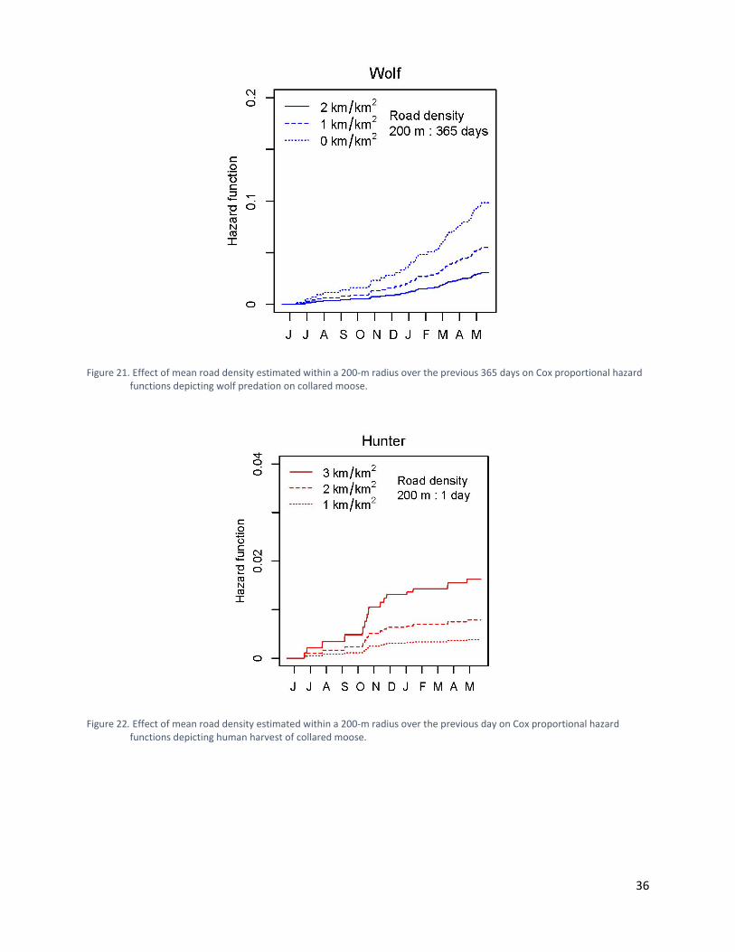
Figure 23. Effect of the mean proportion of new cutblocks estimated within a 400-m radius over the previous 180 days on Cox proportional hazard functions depicting human harvest of collared moose. ......................................................................................................................... 37

Figure 24. Effect of mean road density estimated within a 200-m radius over the previous 365 days on Cox proportional hazard functions depicting apparent starvation for collared moose. ...................................................................................................................................... 37

Figure 25. Effect of the mean proportion of new cutblocks estimated within a 400-m radius over the previous 180 days on Cox proportional hazard functions depicting apparent starvation for collared moose. .................................................................................................. 38

viii

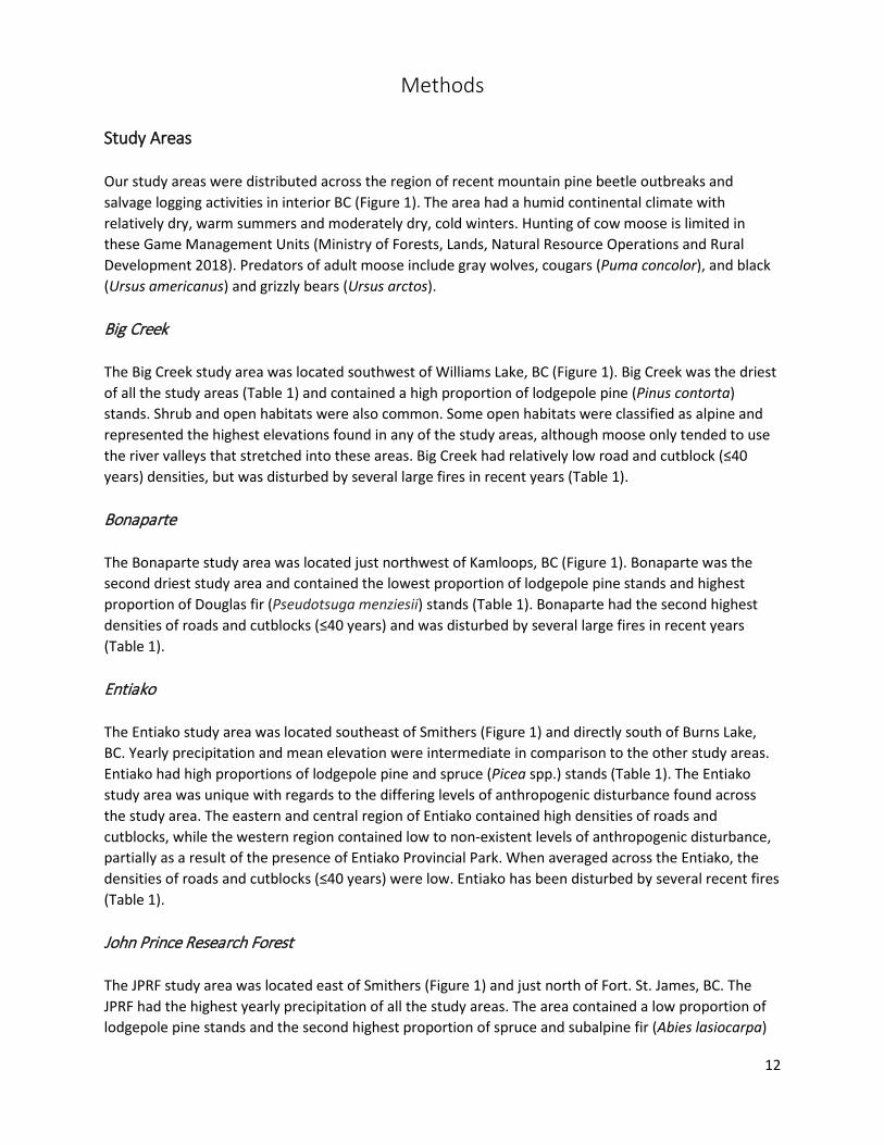
List of Tables Table 1. Proportion of vegetation and disturbance classes, sprayed areas, total area, density of

roads, elevation, and annual precipitation for each study area. Pine = lodgepole pine, Doug. = Douglas, Reg. = regeneration, Adv. = advanced, Cut = cutblocks. .............................. 13

Table 2. Number of cow moose collared in interior British Columbia, along with their fates, transmission rates, and success rates. ...................................................................................... 14

Table 3. Candidate Cox proportional hazards models examining risk to collared moose in British Columbia from wolf predation, human harvest, apparent starvation, and other causes. ....... 24

Table 4. Candidate models used to assess differences between the seasonal habitat use of moose that died of apparent starvation versus individuals that survived or died from other causes. ............................................................................................................................. 26

Table 5. Estimated Kaplan-Meier yearly survival rates for each study area and the average across study areas for collared cow moose in British Columbia.......................................................... 33

Table 6. Simple population model used to estimate the required year one calf survival rates (shaded column) necessary to maintain a stable population of cow moose within our study areas in British Columbia. ............................................................................................... 34

Table 7. Covariates, spatiotemporal scales, hazard ratios, standard errors (SE), Z-values, and P-values for the best-supported Cox proportional hazards model examining risk to cow moose from wolf predation, hunting, apparent starvation, and other causes. ....................... 35

Table 8. Covariate estimates, standard errors (SE), and P-values for the best-supported logistic regression model examining the seasonal influence of habitat use on the probability of apparent starvation. ................................................................................................................. 38

ix

Acknowledgments We thank the Habitat Conservation Trust Foundation and Forest Enhancement Society of British Columbia for funding this research. We also thank the Province of British Columbia and Ministry of Forests, Lands, Natural Resource Operations and Rural Development for funding the majority of the data collection and field activities. We thank Doug Heard and Gerry Kuzyk for their efforts in initiating and facilitating the cow moose survival study. We also thank the many current and former provincial employees that contributed their time, efforts, and insights to this research including Morgan Anderson, Adrian Batho, Alex Bevington, Becky Cadsand, Pat Dielman, Krystal Dixon, Mike Klaczek, Bill Jex, Daniel Lirette, Bryan MacBeth, Shelley Marshall, Cait Nelson, Mark Parminter, Dean Peard, Chris Procter, Matt Scheideman, Heidi Schindler, Helen Schwantje, Conrad Thiessen, Glen Watts, Jeff Werner, Shane White, Shari Willmott, and Mark Wong and thank Michael Burwash and Jen Psyllakis for their support. We also thank the Fish and Wildlife Compensation Program and Chelsea Cody for their financial contribution and Wildlife Infometrics and Krista Sittler for their contributed research. We thank Dexter Hodder, Shannon Crowley, and Jason Mattess for their efforts in the John Prince Research Forest study area. We also appreciate the contributions of Tsilhqot'in National Government, Tl'azt'en Nation, Nak'azdli Whut'en, T’kemlups Indian Band, and Skeetchestn Indian Band. We thank Cliffs Natural Resources, Spectra Energy, Tanizul Timber Ltd, TransCanada Corp, and West Fraser Timber Co. for their support and recognize the contributions of Altoft Helicopter Services Ltd., Canada Helicopters Ltd., Frontline Helicopters Ltd., Qwest Helicopters Inc., Summit Helicopters, White River Helicopters, and Yellowhead Helicopters Ltd. We also thank Greg Altoft, Rob Altoft, Gene Cooper, Brad Culling, Luke Doxtator, Gerad Hales, Francis Iredale, Matt Erickson, Doug Jury, Kirk Miller, Sally Sellers, and Alicia Woods. We thank the University of Northern British Columbia for their support, Kathy Parker for her insights, and Fulbright Canada for their financial contribution. We also thank the Earth Resources Observation and Science Center of the United States Geological Survey for use of the Landsat data layers and the European Space Agency for use of the Sentinel data layers.

10

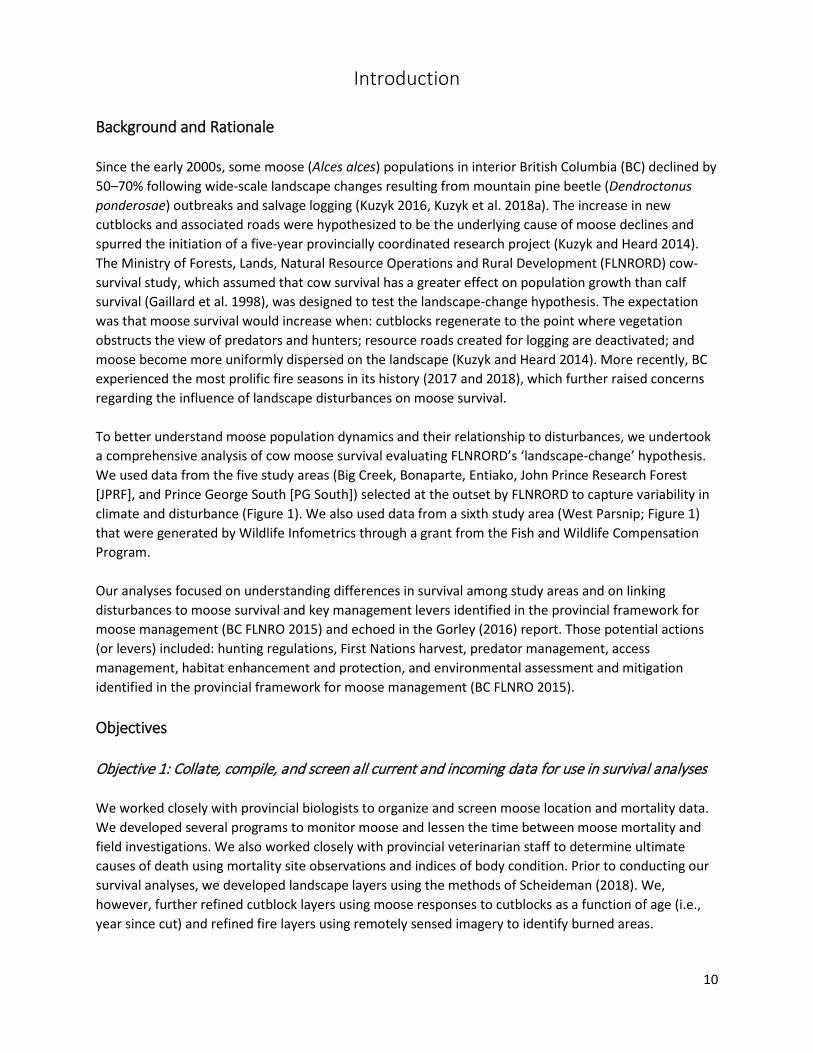
Introduction Background and Rationale Since the early 2000s, some moose (Alces alces) populations in interior British Columbia (BC) declined by 50–70% following wide-scale landscape changes resulting from mountain pine beetle (Dendroctonus ponderosae) outbreaks and salvage logging (Kuzyk 2016, Kuzyk et al. 2018a). The increase in new cutblocks and associated roads were hypothesized to be the underlying cause of moose declines and spurred the initiation of a five-year provincially coordinated research project (Kuzyk and Heard 2014). The Ministry of Forests, Lands, Natural Resource Operations and Rural Development (FLNRORD) cow-survival study, which assumed that cow survival has a greater effect on population growth than calf survival (Gaillard et al. 1998), was designed to test the landscape-change hypothesis. The expectation was that moose survival would increase when: cutblocks regenerate to the point where vegetation obstructs the view of predators and hunters; resource roads created for logging are deactivated; and moose become more uniformly dispersed on the landscape (Kuzyk and Heard 2014). More recently, BC experienced the most prolific fire seasons in its history (2017 and 2018), which further raised concerns regarding the influence of landscape disturbances on moose survival. To better understand moose population dynamics and their relationship to disturbances, we undertook a comprehensive analysis of cow moose survival evaluating FLNRORD’s ‘landscape-change’ hypothesis. We used data from the five study areas (Big Creek, Bonaparte, Entiako, John Prince Research Forest [JPRF], and Prince George South [PG South]) selected at the outset by FLNRORD to capture variability in climate and disturbance (Figure 1). We also used data from a sixth study area (West Parsnip; Figure 1) that were generated by Wildlife Infometrics through a grant from the Fish and Wildlife Compensation Program. Our analyses focused on understanding differences in survival among study areas and on linking disturbances to moose survival and key management levers identified in the provincial framework for moose management (BC FLNRO 2015) and echoed in the Gorley (2016) report. Those potential actions (or levers) included: hunting regulations, First Nations harvest, predator management, access management, habitat enhancement and protection, and environmental assessment and mitigation identified in the provincial framework for moose management (BC FLNRO 2015). Objectives Objective 1: Collate, compile, and screen all current and incoming data for use in survival analyses We worked closely with provincial biologists to organize and screen moose location and mortality data. We developed several programs to monitor moose and lessen the time between moose mortality and field investigations. We also worked closely with provincial veterinarian staff to determine ultimate causes of death using mortality site observations and indices of body condition. Prior to conducting our survival analyses, we developed landscape layers using the methods of Scheideman (2018). We, however, further refined cutblock layers using moose responses to cutblocks as a function of age (i.e., year since cut) and refined fire layers using remotely sensed imagery to identify burned areas.

11

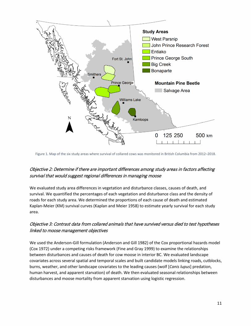
Figure 1. Map of the six study areas where survival of collared cows was monitored in British Columbia from 2012–2018.

Objective 2: Determine if there are important differences among study areas in factors affecting survival that would suggest regional differences in managing moose We evaluated study area differences in vegetation and disturbance classes, causes of death, and survival. We quantified the percentages of each vegetation and disturbance class and the density of roads for each study area. We determined the proportions of each cause of death and estimated Kaplan-Meier (KM) survival curves (Kaplan and Meier 1958) to estimate yearly survival for each study area. Objective 3: Contrast data from collared animals that have survived versus died to test hypotheses linked to moose management objectives We used the Anderson-Gill formulation (Anderson and Gill 1982) of the Cox proportional hazards model (Cox 1972) under a competing risks framework (Fine and Gray 1999) to examine the relationships between disturbances and causes of death for cow moose in interior BC. We evaluated landscape covariates across several spatial and temporal scales and built candidate models linking roads, cutblocks, burns, weather, and other landscape covariates to the leading causes (wolf [Canis lupus] predation, human harvest, and apparent starvation) of death. We then evaluated seasonal relationships between disturbances and moose mortality from apparent starvation using logistic regression.

12

Methods Study Areas Our study areas were distributed across the region of recent mountain pine beetle outbreaks and salvage logging activities in interior BC (Figure 1). The area had a humid continental climate with relatively dry, warm summers and moderately dry, cold winters. Hunting of cow moose is limited in these Game Management Units (Ministry of Forests, Lands, Natural Resource Operations and Rural Development 2018). Predators of adult moose include gray wolves, cougars (Puma concolor), and black (Ursus americanus) and grizzly bears (Ursus arctos). Big Creek The Big Creek study area was located southwest of Williams Lake, BC (Figure 1). Big Creek was the driest of all the study areas (Table 1) and contained a high proportion of lodgepole pine (Pinus contorta) stands. Shrub and open habitats were also common. Some open habitats were classified as alpine and represented the highest elevations found in any of the study areas, although moose only tended to use the river valleys that stretched into these areas. Big Creek had relatively low road and cutblock (≤40 years) densities, but was disturbed by several large fires in recent years (Table 1). Bonaparte The Bonaparte study area was located just northwest of Kamloops, BC (Figure 1). Bonaparte was the second driest study area and contained the lowest proportion of lodgepole pine stands and highest proportion of Douglas fir (Pseudotsuga menziesii) stands (Table 1). Bonaparte had the second highest densities of roads and cutblocks (≤40 years) and was disturbed by several large fires in recent years (Table 1). Entiako The Entiako study area was located southeast of Smithers (Figure 1) and directly south of Burns Lake, BC. Yearly precipitation and mean elevation were intermediate in comparison to the other study areas. Entiako had high proportions of lodgepole pine and spruce (Picea spp.) stands (Table 1). The Entiako study area was unique with regards to the differing levels of anthropogenic disturbance found across the study area. The eastern and central region of Entiako contained high densities of roads and cutblocks, while the western region contained low to non-existent levels of anthropogenic disturbance, partially as a result of the presence of Entiako Provincial Park. When averaged across the Entiako, the densities of roads and cutblocks (≤40 years) were low. Entiako has been disturbed by several recent fires (Table 1). John Prince Research Forest The JPRF study area was located east of Smithers (Figure 1) and just north of Fort. St. James, BC. The JPRF had the highest yearly precipitation of all the study areas. The area contained a low proportion of lodgepole pine stands and the second highest proportion of spruce and subalpine fir (Abies lasiocarpa)

13

Table 1. Proportion of vegetation and disturbance classes, sprayed areas, total area, density of roads, elevation, and annual

precipitation for each study area. Pine = lodgepole pine, Doug. = Douglas, Reg. = regeneration, Adv. = advanced, Cut = cutblocks.

Study Area

Pine (%)

Spruce (%)

Fir (%)

Doug. Fir (%)

Broad (%)

Shrub (%)

Open (%)

Wetland (%)

Water (%)

West Parsnip 16 28 21 0 3 7 4 1 4 JPRF 9 26 9 3 7 8 1 3 9 Entiako 26 25 7 0 1 6 6 2 7 PG South 17 16 1 2 8 8 6 3 3 Big Creek 27 4 1 3 2 11 18 2 3 Bonaparte 5 11 2 15 3 6 7 1 4

Study Area

New Burn (%)

Reg. Burn (%)

Adv. Burn (%)

Total Burn (%)

New Cut (%)

Reg. Cut (%)

Adv. Cut (%)

Total Cut (%)

Sprayed Areas (%)

West Parsnip <1 <1 <1 <1 6 4 5 16 <1 JPRF <1 <1 <1 <1 10 8 6 24 <1 Entiako 10 1 0 11 2 5 0 7 <1 PG South 5 1 <1 7 6 16 6 28 2 Big Creek 13 3 <1 16 4 5 5 14 0 Bonaparte 16 2 <1 18 9 13 6 28 <1

Study Area

Total Area (km2)

Road Density (km/km2)

Elevation Mean (m)

Elevation Range (m)

Precipitation Mean (mm)

Precipitation Range (mm)

West Parsnip 11487 0.78 1122 665–2169 467 379–539 JPRF 9067 1.11 934 676–1979 497 361–673 Entiako 15248 0.52 1135 717–2257 428 337–533 PG South 9942 1.89 924 507–1617 468 393–591 Big Creek 9404 0.91 1494 527–3057 292 211–387 Bonaparte 6009 1.63 1195 333–1871 378 243–487

stands (Table 1). The JPRF had the third highest densities of roads and cutblocks (≤40 years). The proportion of burned areas was low (Table 1). Prince George South The PG South study area was located southwest of Prince George, BC (Figure 1). The PG South was one of the wetter study areas (Table 1). The PG South contained high proportions of lodgepole pine and spruce leading stands (Table 1). The PG South has the highest road densities and the highest proportions of cutblocks (≤40 years) and was recently disturbed by several fires (Table 1).

14

West Parsnip The West Parsnip study area was located between Smithers and Fort St. John, BC (Figure 1), just west of the southern portion of the Williston Reservoir. West Parsnip had high yearly precipitation and high proportions of lodgepole pine, spruce, and subalpine fir stands (Table 1). The densities of roads and cutblocks (≤40 years) were low to intermediate and the proportion of burned areas was low (Table 1). Collaring and Monitoring of Collared Moose Cow Moose Collaring, Fates, Transmission Rates, and Success Rates The Province of BC oversaw the capture of adult female moose each winter from 2012–2018 (2012 Bonaparte only) and affixed each individual with GPS-telemetry collars in accordance with the British Columbia Wildlife Act under permit CB17-277227. Four hundred and fifty-six moose were collared across the six study areas (Table 2). The rate of transmission varied between collars and ranged from 1–16 locations/day. Transmission success rates ranged from 0.60–0.85 with a mean value across study areas of 0.76. Analysis of data from recovered GPS collars suggested that low fix success was associated with satellite uploading rather than with GPS-fix acquisition. As of July 31, 2018, 121 moose had succumbed from some form of mortality. Out of the remaining individuals, 230 of the collars were still active and 105 were no longer transmitting locations (Table 2). Individuals were regularly monitored and investigations were prompted when collars exhibited little or no movement (see Screening for mortalities). Five individuals were censored from the study because of collar failure or death <1 month after collaring to remove potential capture-related deaths (Table 2). Table 2. Number of cow moose collared in interior British Columbia, along with their fates, transmission rates, and success

rates.

Study Area Total Dead Censored Transmission Rates Success Rates Big Creek 65 20 0 4, 12, 24 0.85 Bonaparte 142 22 2 1.5, 4, 12 0.72 Entiako 77 33 1 3, 4, 6, 12, 24 0.85 JPRF 48 9 0 12,14 0.60 PG South 70 25 1 4, 12, 24 0.80 West Parsnip 54 12 1 24 0.74 Total 456 121 5 1.5, 3, 4, 6, 12, 24 0.76

Screening for Mortalities All collars were equipped with a motion-sensitive device that triggered a mortality signal once a collar remained stationary for >4, >8, or >12 hours depending on the collar. At times, however, collars failed to go into mortality mode potentially because of collar malfunction or the continued movement of the collar by predators or scavengers following a mortality. In other cases, seasonal inactivity triggered mortality signals when moose were still alive. We, therefore, developed an Excel macro to monitor moose and identify potential mortalities, thus lessening the time between mortality investigations and

15

time of death. In addition to limited movement, the macro signaled mortality warnings in response to long distance movements followed by little movement or the missed transmission of location(s). The underlying parameters with regards to movement distances could be set and adjusted for various collar transmission rates (Figure 2) and generated a file that could be viewed in Google Earth for a visual evaluation of potential mortalities (Figure 3). For much of the study, locations were downloaded at least weekly and run through the macro to assist in determining the appropriate response to mortality signals and other warnings generated by the macro.

Figure 2. Parameter settings of Excel macros used to identify mortalities via changes in moose movement.

Mortality Site Investigations and Proximate Cause of Death Suspected mortality events were investigated by provincial biologists to determine cause of death. Biologists gathered information in a standardized manner ( see Appendix 1) and assigned a proximate cause of death using observations from the mortality site, such as evidence of reduced health or condition, evidence of predator or scavenger consumption, predator scats or tracks, and signs of a chase or struggle. When possible, samples were also collected from mortality locations and sent to provincial veterinarian staff to evaluate moose age, health, and condition and test predator scats for species identification. We coordinated with biologists to gather mortality observation forms and ensure data accuracy by reviewing mortality observations and proximate cause of death assignments, and by cross-checking transmitted collar locations against recorded mortality locations.

16

Figure 3. Example of Google Earth output from Excel macro used to identify mortality via changes in moose movement.

Determination of Ultimate Cause of Death Once sample testing from provincial veterinarian staff was completed, we re-evaluated mortalities to determine ultimate causes of death by considering field observations, proximate causes of death, and the further information provided by sample testing. Results from collected samples provided moose age and indices of disease and condition, such as % bone marrow fat from moose femurs, humeri, or jaw bones. Percent bone marrow fat has been used in other studies as a measure of ungulate condition and used to reassign apparent predation events to health- and condition-related deaths (Gasaway et al. 1992). To reduce subjectivity in assigning ultimate causes of death, we developed a flow chart (Figure 4) with consultation from provincial biologists and veterinarian staff to guide decision-making. We used this flow chart to determine the ultimate cause of death for each moose mortality and further consulted provincial veterinarian staff as needed. We defined the ultimate cause of death as the underlying reason an animal died or was susceptible to death from a proximate cause. For example, a moose in extremely poor body condition might be killed by a bear, but might have died regardless; thus the ultimate cause of death for this individual would be apparent starvation (unless disease or a prior injury was detected). We set 20% bone marrow fat as the threshold at which deaths from predation were reassigned to apparent starvation, which was consistent with prior research (Peterson et al. 1984). Ultimate causes of death in our flow chart included wolf predation, failed (attempted) wolf predation, bear predation, cougar predation, failed (attempted) cougar predation, unknown predator, failed (attempted) unknown predator, licensed hunter, unlicensed hunter, apparent starvation, health-related, natural accident, unnatural (anthropogenic) accident, and unknown cause (Figure 4).

17

Figure 4. Flow chart used to determine ultimate cause of death for collared moose mortality.

18

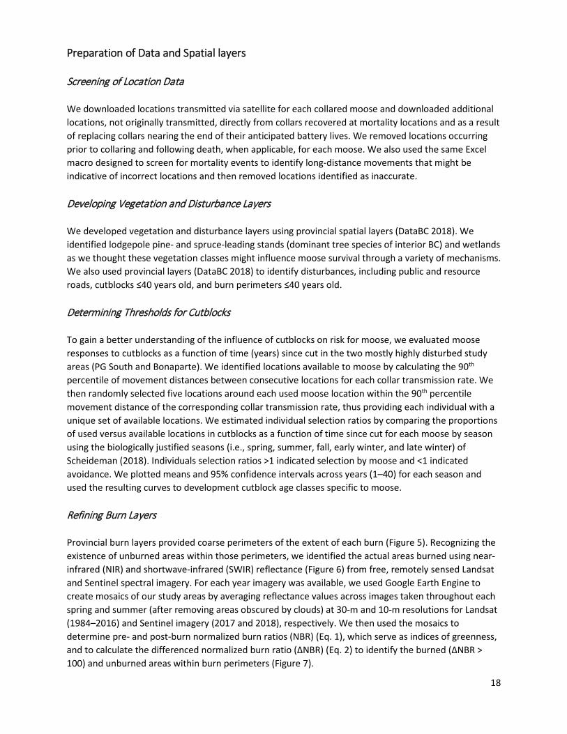
Preparation of Data and Spatial layers Screening of Location Data We downloaded locations transmitted via satellite for each collared moose and downloaded additional locations, not originally transmitted, directly from collars recovered at mortality locations and as a result of replacing collars nearing the end of their anticipated battery lives. We removed locations occurring prior to collaring and following death, when applicable, for each moose. We also used the same Excel macro designed to screen for mortality events to identify long-distance movements that might be indicative of incorrect locations and then removed locations identified as inaccurate. Developing Vegetation and Disturbance Layers We developed vegetation and disturbance layers using provincial spatial layers (DataBC 2018). We identified lodgepole pine- and spruce-leading stands (dominant tree species of interior BC) and wetlands as we thought these vegetation classes might influence moose survival through a variety of mechanisms. We also used provincial layers (DataBC 2018) to identify disturbances, including public and resource roads, cutblocks ≤40 years old, and burn perimeters ≤40 years old. Determining Thresholds for Cutblocks To gain a better understanding of the influence of cutblocks on risk for moose, we evaluated moose responses to cutblocks as a function of time (years) since cut in the two mostly highly disturbed study areas (PG South and Bonaparte). We identified locations available to moose by calculating the 90th percentile of movement distances between consecutive locations for each collar transmission rate. We then randomly selected five locations around each used moose location within the 90th percentile movement distance of the corresponding collar transmission rate, thus providing each individual with a unique set of available locations. We estimated individual selection ratios by comparing the proportions of used versus available locations in cutblocks as a function of time since cut for each moose by season using the biologically justified seasons (i.e., spring, summer, fall, early winter, and late winter) of Scheideman (2018). Individuals selection ratios >1 indicated selection by moose and <1 indicated avoidance. We plotted means and 95% confidence intervals across years (1–40) for each season and used the resulting curves to development cutblock age classes specific to moose. Refining Burn Layers Provincial burn layers provided coarse perimeters of the extent of each burn (Figure 5). Recognizing the existence of unburned areas within those perimeters, we identified the actual areas burned using near-infrared (NIR) and shortwave-infrared (SWIR) reflectance (Figure 6) from free, remotely sensed Landsat and Sentinel spectral imagery. For each year imagery was available, we used Google Earth Engine to create mosaics of our study areas by averaging reflectance values across images taken throughout each spring and summer (after removing areas obscured by clouds) at 30-m and 10-m resolutions for Landsat (1984–2016) and Sentinel imagery (2017 and 2018), respectively. We then used the mosaics to determine pre- and post-burn normalized burn ratios (NBR) (Eq. 1), which serve as indices of greenness, and to calculate the differenced normalized burn ratio (ΔNBR) (Eq. 2) to identify the burned (ΔNBR > 100) and unburned areas within burn perimeters (Figure 7).

19

Figure 5. Perimeter of Little Bobtail Lake Fire, which burned within the PG South study area in 2015.

NBR = NIR-SWIR/NIR+SWIR Eq. 1

ΔNBR = pre-burn NBR – post-burn NBR Eq. 2

20

Figure 6. Schematic comparing wavelength (Electromagnetic Spectrum) of pre- and post-burn images (source www.fs.fed.us).

Figure 7. Estimate of burned and unburned areas within the perimeter of the Little Bobtail Lake fire (2015) as determined via differenced normalized burn ratios using spectral imagery.

21

Causes of Death and Survival Estimates by Study Area Determining Kaplan-Meier Survival Curves We fit KM survival curves to estimate and compare cow moose survival rates between study areas. For each study area, we determined daily survival rates from KM survival curves and then multiplied daily survival by 365.25 days to estimate yearly survival. Estimating Demographic Rates Required to Achieve Population Stability To examine the potential implications of estimated cow survival rates on the population growth of each study area, we constructed a simple population growth model. The model permitted us to gain some information with regards to the calf survival rates (from birth through one year of age) required to maintain stable populations. Our model assumed that to achieve population stability there must be enough calves surviving until age two (likely minimum breeding age) in order to offset losses from adult cow mortalities. We were highly conservative in our modelling approach and set several of the parameters at values that likely exceeded the true population parameters, thus our estimates of calf survival likely represent the minimum rates necessary to achieve population stability. During the course of the study, annual pregnancy rates across the study areas ranged from 0.64–0.94 with a mean of 0.79 (Kuzyk et al. 2018b). Information on twinning rates was not available, but was assumed to be low. In our model, we set cow pregnancy rates to 1, which assumed 90% pregnancy and ~10% twinning. We also assumed a 1:1 ratio of male to female calves, thus equaling 0.5 female calves for every pregnant cow moose. We set the yearling female survival rates to that of adult females, which was likely higher than the actual yearling survival rate. Modelling Risk with Cox Proportional Hazards Models Description of Model Following the determination of ultimate causes of mortality, it was apparent that cow moose died from multiple causes of death. We hypothesized that these mortality agents might be influenced by disturbances in different ways. We, therefore, implemented a cause-specific approach (Heisey and Patterson 2006) to understanding risk for moose in BC. To preserve statistical power, we combined wolf predation and attempted wolf predation and separately combined licensed and unlicensed hunting. We created an ‘other causes’ category by combining minor causes of death, namely bear predation, cougar predation, attempted cougar predation, attempted unknown predator, health-related, anthropogenic accident, natural accident, and unknown cause. This resulted in four categorical causes of death: wolf predation, human harvest, apparent starvation, and other causes. The cause-specific approach requires that the dataset is replicated for each cause of death. In each replicate, one cause of death is preserved while the remaining causes are censored. The replicated data sets are then combined. This data structure, known as data augmentation, allows for separate coefficients to be estimated for each covariate in relation to each cause of death. We used the Anderson-Gill formulation (Anderson and Gill 1982) of the Cox proportional hazards model (Cox 1972) to evaluate the influence of disturbances on risk (causes of moose mortality) for moose. Cox proportional hazards models estimate the influence of covariates on a baseline hazard function. This

22

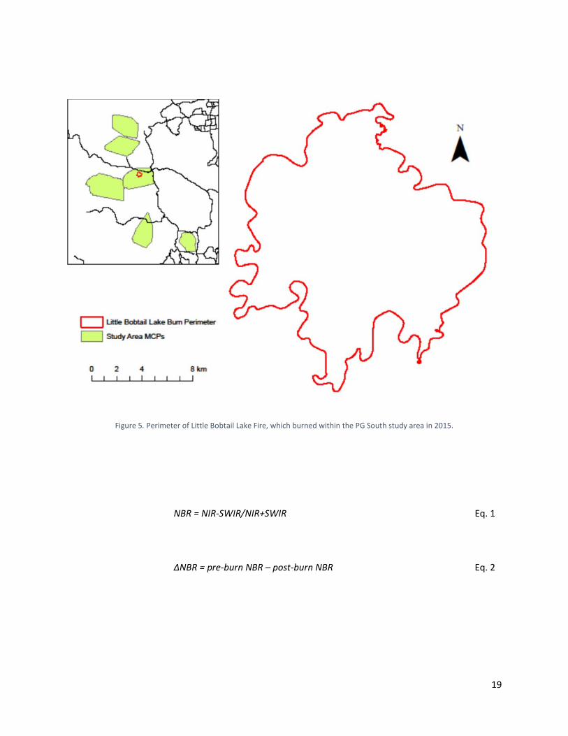
hazard function represents the cumulative rate of mortality through time. Our models included separate hazard functions for each cause of death (i.e., wolf predation, human harvest, apparent starvation, and other causes). Coefficients for individual covariates can be presented as hazard ratios, representing the proportional change in the hazard function in response to covariate values. Hazard ratios >1 indicate an increase in risk, and hazard ratios <1 indicate a decrease in risk. Development of Covariates and Candidate Models Disturbances of interest included roads, cutblocks, sprayed cutblocks, and burns. We hypothesized that those disturbances might influence risk for moose across different spatial and temporal scales. In particular, we thought some causes of death were likely to be influenced over short periods of time (i.e., wolf predation and human harvest), while others might be the result of a long-term process (i.e, apparent starvation). We, therefore, estimated the density of roads and the proportions of new cutblocks (1–8 years), regenerating cutblocks (9–24 years), sprayed cutblocks, and new burns (1–8 years), and regenerating burns at 200-m, 400-m, 800-m, and 1600-m radii around each moose location. We captured temporal aspects of risk by back-calculating mean values of each spatial scale at 1-, 7-, 14-, 90-, 180-, and 365-day windows (Figure 8). We considered the 90-, 180-, and 365-day windows to be estimates of the disturbances present within the seasonal, half-year, and yearly weighted home ranges of each moose on any given day.

Figure 8. Schematic illustrating the spatial and temporal scales used in survival modelling. Each collared moose location was used to query several underlying covariates (list on left slide of figure) within 200-, 400-, 800-, and 1600-m radii. The values of each covariate at each spatial scale were then back-calculated for 1-, 7-, 14-, 90-, 180-, and 365-day windows.

23

Additional covariates included the proportions of wetlands, lodgepole pine-leading (pine) stands, and spruce-leading (spruce) stands, along with several weather covariates thought to potentially relate to apparent starvation. We estimated the proportions of wetlands, pine, and spruce stands around each moose location for every spatial by temporal scale. We extracted daily precipitation and temperature data from weather stations (PCIC 2018) for each study area (no spatial variation within study areas). We thought precipitation might influence forage growth, but also hypothesized that precipitation during the winter (likely snow) might increase the energetic costs of movement (Peek 1971). We also hypothesized that temperature might influence forage and energetic costs for moose. We estimated growing degree days (base temperature equaled 10 °C) for each day during the growing season, which provided an index of the rate of plant growth. Moose can incur greater energetic costs via heat stress as a result of temperature (Renecker and Hudson 1986), but temperature thresholds at which animals experience stress varies dependent upon solar exposure, humidity, and wind speed (Parker and Gillingham 1990). For moose, temperature thresholds also vary widely in response to seasonal coat thickness (-5–0 °C in summer and 14–20 °C in winter) (Renecker and Hudson 1986, Dussault et al. 2004). We took a conservative approach to identifying temperature thresholds and determined days when the mean daily temperature exceeded 20 °C in the growing period (spring and summer) and 0 °C during the non-growing period (fall, early winter, and late winter). We calculated the mean values for each weather covariate at each temporal scale. Prior to developing models, we compared log-likelihood values between univariate models to identify the most informative spatial (200-, 400-, 800-, or 1600-m radius) by short-term temporal scale (1-, 7-, or 14-day window) and spatial (200-, 400-, 800-, or 1600-m radius) by long-term temporal scale (90-, 180-, or 365-day window) for each covariate. We then used the most informative scales of each covariate to build candidate models and selected the best-supported models using an information theoretic approach (<2 ΔAIC, Burnham and Anderson 2002). Each model was specific to theorized mechanisms relating disturbances to causes of death (Table 3). We removed regenerating burns from all models, because of model convergence issues resulting from the scarcity of regenerating burns within our study areas. Evaluating Seasonal Space Use and Apparent Starvation Covariates and Candidate Models Following our cause-specific analysis of risk, we were interested in further exploring apparent starvation to tease apart potential relationships between seasonal habitat use and risk from apparent starvation. Because we lacked information on habitat use during previous seasons for individuals that died <1 year after collaring, we limited our dataset to individuals that survived >1 year post-capture. For individuals that survived across multiple years, we randomly selected a single year for the analysis. We wanted to calculate habitat use while accounting for differences in our knowledge of the areas used and available to individuals as a result of differing collar transmission rates (1, 2, 4, 6, 8, and 16 locations/day). We started by determining the 90th percentile of movement distances (~200 m) between consecutive locations for collars that transmitted 16 locations/day (Figure 9). The total area sampled for 16 non-overlapping locations with a radius of 200 m was ~2 km2, so we set radii for all other transmission rates to achieve an equivalent daily sample (~2 km2). This resulted in radii of 283, 327, 400, 566, and 800 m for transmission rates of 8, 6, 4, 2, and 1 locations/day, respectively. For each individual, we calculated the daily use of road densities and the proportions of new cutblocks, regenerating cubtlocks, and new

24

Table 3. Candidate Cox proportional hazards models examining risk to collared moose in British Columbia from wolf predation, human harvest, apparent starvation, and other causes.

Cause(s) of

death Model Covariates (temporal scale) Mechanism(s) W

olf p

reda

tion

and

hu

ntin

g Access Road density (short) Increased access Access and visibility Road density (short), new

cutblocks (short), new burns (short)

Increased access and visibility

Access to new cutblocks

Road density (short) × new cutblocks (short)

Increased access to areas with high visibility

Access to wetlands Road density (short) × wetlands (short)

Increased access to areas selected by moose (i.e., wetlands)

Appa

rent

star

vatio

n

Heat stress New cutblocks (long), days >temp. threshold (long)

Increased heat stress via decreased cover and temperature

Snow interception New cutblocks (long), winter precip. (long)

Increased energetic costs via snow interception

Altered forage 1 New cutblocks (long), reg. cutblocks (long), precip (long)

Altered forage via disturbances and weather

Altered forage 2 New cutblocks (long), reg. cutblocks (long), new burns (long)

Altered forage via disturbances

Altered forage 3 Precip. (long), growing degree days (long)

Altered forage via weather

Wol

f pre

datio

n, h

untin

g, a

nd

appa

rent

star

vatio

n

Access, visibility, and forage 1

Road density (short/long), new cutblocks (long/short)

Increased access and visibility, altered forage

Access, visibility, and forage 2

Road density (short), new cutblocks (short/long), new burns (short/long)

Increased access and visibility, altered forage

Visibility, forage, and heat stress

New cutblocks (short/long), days >temp. threshold (long)

Increased visibility, altered forage, increased heat stress

Visibility and forage 1 New cutblocks (short/long), precipitation (long), growing degree days (long)

increased visibility, altered forage

Visibility and forage 2 New cutblocks (short/long) and new burns (long/short)

Increased visibility, altered forage

burns using the appropriate spatial scale. We also calculated the proportions of wetlands, pine stands, and spruce stands. We then used those daily estimates of habitat use to determine the seasonal (i.e., spring, summer, fall, early winter, and late winter) habitat use of each individual.

25

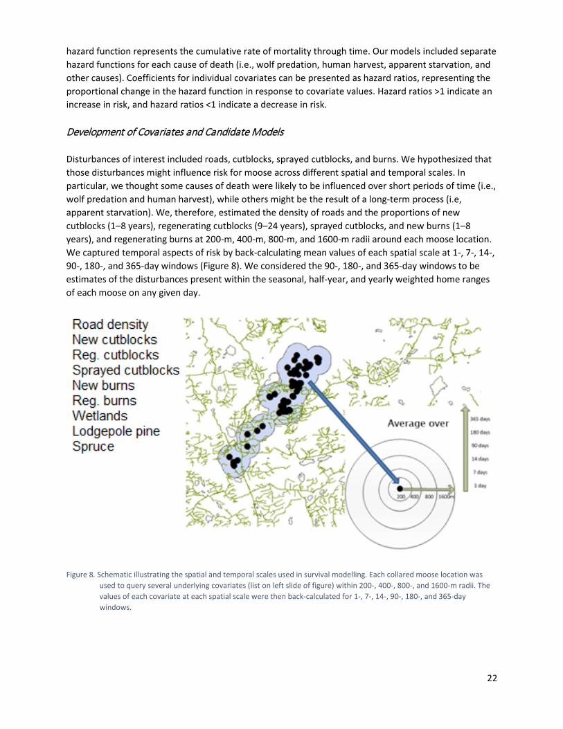
Figure 9. Schematic of buffered areas around location points (see text) used to assess use by collared cow moose. We built candidate logistic regression models and selected the best-supported models using an information theoretic approach (<2 ΔAIC, Burnham and Anderson 2002). These models represented hypothesized mechanisms linking habitat use during previous seasons to the risk of dying from apparent starvation (Table 4). We grouped our seasons into the vegetative growing period (spring and summer) and non-growing period (fall, early winter, and late winter). Within the suite of models for the non-growing period, we also included a snow-interception model, which only used covariates estimates across early and late winter (Table 4).

Results Causes of Mortality Ultimate Cause of Death In conjunction with provincial biologists and veterinarian staff, we assessed the cause of death for all 121 mortalities. We reassigned three mortalities with a bear (n = 2) or wolf (n = 1) proximate cause of death to apparent starvation, because of <20% bone marrow fat at time of death. Because of a leg injury, we reassigned another bear proximate cause of death with <20% bone marrow fat to anthropogenic accident. The data did not indicate that predators were killing older, weaker moose (Figure 10). Ultimate causes of death included anthropogenic accident (Anth_Accid), natural accident (accident), apparent starvation (App_Starv), health related (Health), licensed hunting (L_Hunting), unlicensed hunting (U_Hunting), bear predation (Bear_Pred), cougar predation (Coug_Pred), attempted

26

Table 4. Candidate models used to assess differences between the seasonal habitat use of moose that died of apparent

starvation versus individuals that survived or died from other causes.

Period Model Covariates (seasons) Mechanism Gr

owin

g

Road disturbance Road density (spring–summer) Increased energetic demands via increased movement or stress

Heat stress New cutblocks, new burns, spruce, pine (spring–summer)

Altered heat stress via available canopy cover

Altered forage New cutblocks, reg. cutblocks, new burns (spring–summer)

Altered forage via disturbances

Available forage New cutblocks, reg. cutblocks, new burns, wetlands, spruce, pine (spring–summer)

Available forage via disturbances and intact vegetation classes

Spraying Sprayed cutblocks (spring–summer)

Decreased forage via spraying

Non

-gro

win

g

Road disturbance Road density (fall–early winter–late winter)

Increased energetic demands via increased movement or stress

Heat stress New cutblocks, new burns, spruce, pine (fall–early winter–late winter)

Altered heat stress via available canopy cover

Altered forage New cutblocks, reg. cutblocks, new burns (fall–early winter–late winter)

Altered forage via disturbances

Available forage New cutblocks, reg. cutblocks, new burns, spruce, pine (fall–early winter–late winter)

Available forage via disturbances and intact vegetation classes

Snow interception New cutblocks, new burns, spruce, pine (early winter–late winter)

Altered snow depths via changes in snow interception

cougar predation (F_Coug_Pred), wolf predation (Wolf_Pred), attempted wolf predation (F_Wolf_Pred), attempted unknown predator (Failed_Pred), unknown predation (Unk_Pred), and unknown cause (Unknown) (Figure 11). Attempted cougar predation, attempted wolf predation, and attempted unknown predator ultimate causes of death were identified via the presence of older bite wounds thought to have caused death several weeks after a predator attack. After combining categories (blue brackets in Figure 11), we observed that wolf predation (n = 51) was the most common ultimate cause of death, followed by apparent starvation (n = 17) and human harvest (n = 16) (Figure 12).

27

Figure 10. Known age of collared cow moose by ultimate cause of mortality. Age was obtained by sectioning teeth for all

mortalities where teeth were recovered.

Figure 11. Breakdown of ultimate cause of death for collared cow moose in British Columbia.

28

Figure 12. Pooled ultimate causes of death for collared cow moose in British Columbia. Some causes of death demonstrated strong seasonal patterns. Apparent starvation primarily occurred from late winter through spring, which was similar to the timing of bear predation. Notably, spring is also the time of year when moose calves are expected to be most vulnerable to bear predation (Zager and Beecham 2006). Human harvest peaked in the fall, but also occurred at other times of year. Wolf predation occurred year-round, but was most common during winter (Figure 13).

Figure 13. Month of the year when the four most common sources of ultimate mortality of collared cow moose occurred.

29

Refined Cutblock and Burn Layers When evaluating moose responses as a function of time (years) since cut, we observed that moose generally avoided newer cutblocks, selected (or use equal to availability) regenerating cutblocks, and avoided older cutblocks (Figure 14). The breakpoints between these responses (avoidance–selection–avoidance), however, varied across seasons. Averaging those breakpoints, set our thresholds for new cutblocks at 1–8 years since cut and for regenerating cutblocks at 9–24 years since cut. We used the same age classes to define burns.

Figure 14. Selection ratios (and 95% confidence intervals) as a function of time (years) since cut for moose (right axis) in British Columbia.

Across our study areas, we observed recent increases in the proportion of cutblocks and burns. Following mountain pine beetle outbreaks and coincident with salvage logging, forestry activities in our study areas increased in the early 2000s (Figure 15). The cumulative effect of that increase doubled the proportion of the landscape comprised of new and regenerating cutblocks (Figure 15). The amount of area burned in recent years followed a similar, but more extreme pattern. Our use of ΔNBR to redefine burns revealed the existence of unburned areas within burn perimeters (Figure 16).

30

Figure 15. Proportion of areas cut per year and the cumulative proportion of new cutblocks (1–8 years) and regenerating (reg.) cutblocks (9–24 years) in the PG South and Bonaparte study areas.

31

Figure 16. Area of burn perimeters compares to estimates of the areas burned as identified using differenced normalized burn ratios.

Causes of Death and Survival Estimates by Study Area Causes of Death by Study Area Wolf predation occurred in every study area and was the predominant cause of death in five of the study areas (Figure 17). Apparent starvation was the leading cause of death in the Bonaparte and was observed in five of six study areas. Human harvest took place in four study areas (Figure 17) spanning six wildlife management units (Figure 18). Kaplan-Meier Survival Estimates

Kaplan-Meier survival curves demonstrated differences in survival rates between study areas (Figure 19). The JPRF had the highest yearly survival rate (92.45%) and the Entiako study area had the lowest (81.10%). The average yearly survival rate across study areas was 86.80% (Table 5).

32

Figure 17. Ultimate causes of mortality for collared moose in British Columbia by study area. Apparent starvation is displayed by the detached portion of the pie diagrams.

Figure 18. Frequency of licensed and unlicensed hunting by Game Management Unit for collared cow moose in British Columbia.

33

Figure 19. Comparison of Kaplan-Meier survival estimates for all six study areas in which cow moose were collared. The start of collaring differed among study areas with Bonaparte beginning earliest (late winter 2012) and West Parsnip beginning latest (late winter 2017).

Table 5. Estimated Kaplan-Meier yearly survival rates for each study area and the average across study areas for collared cow

moose in British Columbia. .

Study Area Yearly Survival Big Creek 89.28%

Bonaparte 89.26% Entiako 81.10%

JPRF 92.45% PG South 84.64%

West Parsnip 84.05% Overall (averaged) 86.80 ± 4.22 (SD)%

Demographic Rates for Population Stability Our conservative estimates of the required year 1 calf survival rates necessary to maintain stable populations of cow moose in each study area demonstrated higher variability than our estimates of cow moose survival (Table 6). The JPRF demonstrated the lowest minimum calf survival rate required to achieve stability (0.18), followed by Big Creek and Bonaparte (0.27). Prince George South (0.43), Bonaparte (0.45), and Entiako (0.57) demonstrated higher required rates of year 1 calf survival. The minimum calf survival rate averaged across study areas was 0.35 (Table 6).

34

Table 6. Simple population model used to estimate the required year one calf survival rates (shaded column) necessary to

maintain a stable population of cow moose within our study areas in British Columbia.

Study Area # Cows % Cow survival

Pregnancy rate

Female calves/cow

Year 1 calf

survival

Year 2 calf

survival Replacement

breeding cows Big Creek 100 89.3 1 0.5 0.27 0.893 10.8

Bonaparte 100 89.3 1 0.5 0.27 0.893 10.8 Entiako 100 81.1 1 0.5 0.57 0.811 18.7

JPRF 100 92.5 1 0.5 0.18 0.925 7.7 PG South 100 84.6 1 0.5 0.43 0.846 15.4

West Parsnip 100 84.1 1 0.5 0.45 0.841 15.9 Overall 100 86.8 1 0.5 0.35 0.868 13.2

Cox Proportional Hazard Models of Risk Hazard functions from our risk models demonstrated that wolf predation accounted for the largest proportion of mortality for collared moose (Figure 20). The best-supported model explaining risk to moose from wolf predation, human harvest, apparent starvation, and other causes included covariates for road density and new cutblocks (Table 7). The influence of covariates on certain risks was uncertain as evidenced by hazard ratios that hovered around 1.0 and had large standard errors in comparison to their hazard ratios. All covariates, however, demonstrated strong responses to at least one type of risk (Table 7). The risk of wolf predation was increased for moose that used areas with lower road densities over the previous 365 days (Figure 21, Table 7). The risk from human harvest was increased for moose that used areas with higher road densities on a given day (Figure 22) and a greater proportion of cutblocks during the previous seven days (Figure 23, Table 7). The risk from apparent starvation was increased for moose that used areas with higher road densities over the previous 365 days (Figure 24) and higher proportions of cutblocks over the previous 180 days (Figure 25, Table 7). Seasonal Space Use and Apparent Starvation In our subsequent examination of apparent starvation, the best-supported models examining the relationships between seasonal habitat use and apparent starvation for moose included new cutblocks, new burns, spruce stands, and pine stands. The snow-interception model suggested that the use of areas in early and late winter with higher proportions of cutblocks, new burns, spruce, and pine increased the probability of apparent starvation (Table 8). The Thermal stress model suggested that the use of areas in fall, early winter, and late winter with higher proportions of cutblocks, new burns, and pine increased the probability of apparent starvation (Table 8). Higher proportions of spruce, however, decreased the probability of apparent starvation in the thermal stress model (Table 8).

35

Figure 20. Cox proportional hazard functions for wolf predation, human harvest (hunting), apparent starvation, and other causes for collared cow moose in interior British Columbia.

Table 7. Covariates, spatiotemporal scales, hazard ratios, standard errors (SE), Z-values, and P-values for the best-supported

Cox proportional hazards model examining risk to cow moose from wolf predation, hunting, apparent starvation, and other causes.

Risk Covariate Spatial Scale (m)

Temporal Scale (days)

Hazard Ratio SE Z-value P-value

Wol

f Pr

edat

ion Road Density 200 1 1.00 0.10 -0.02 0.99

Road Density 200 365 0.56 0.23 -2.50 0.01* New Cutblocks 400 7 1.34 1.25 0.23 0.82 New Cutblocks 400 180 0.21 1.98 -0.78 0.44

Hunt

ing Road Density 200 1 1.62 0.15 3.23 <0.01*

Road Density 200 365 1.67 0.41 1.26 0.21 New Cutblocks 400 7 49.06 1.76 2.21 0.03* New Cutblocks 400 180 31.69 2.88 1.20 0.23

Appa

rent

St

arva

tion Road Density 200 1 0.97 0.18 -0.17 0.87

Road Density 200 365 2.60 0.38 2.49 0.01* New Cutblocks 400 7 1.14 1.95 0.07 0.95 New Cutblocks 400 180 555.70 2.90 2.18 0.03*

Oth

er C

ause

Road Density 200 1 1.20 0.13 1.37 0.17 Road Density 200 365 1.60 0.32 1.46 0.14 New Cutblocks 400 7 0.98 2.07 -0.01 0.99 New Cutblocks 400 180 0.27 3.26 -0.40 0.69

36

Figure 21. Effect of mean road density estimated within a 200-m radius over the previous 365 days on Cox proportional hazard functions depicting wolf predation on collared moose.

Figure 22. Effect of mean road density estimated within a 200-m radius over the previous day on Cox proportional hazard functions depicting human harvest of collared moose.

37

Figure 23. Effect of the mean proportion of new cutblocks estimated within a 400-m radius over the previous 180 days on Cox proportional hazard functions depicting human harvest of collared moose.

Figure 24. Effect of mean road density estimated within a 200-m radius over the previous 365 days on Cox proportional hazard functions depicting apparent starvation for collared moose.

38

Figure 25. Effect of the mean proportion of new cutblocks estimated within a 400-m radius over the previous 180 days on Cox proportional hazard functions depicting apparent starvation for collared moose.

Table 8. Covariate estimates, standard errors (SE), and P-values for the best-supported logistic regression model examining the

seasonal influence of habitat use on the probability of apparent starvation.

Model Covariate Estimate SE P-value

Snow

In

terc

eptio

n Intercept -6.47 1.68 <0.01 New Cutblocks 6.88 2.86 0.02 New Burns 4.33 2.11 0.04 Spruce 2.24 3.35 0.50 Lodgepole Pine 8.93 2.81 <0.01

Model Covariate Estimate SE P-value

Ther

mal

Str

ess Intercept -5.43 1.67 <0.01

New Cutblocks 6.01 2.92 0.04 New Burns 3.78 2.13 0.07 Spruce -0.80 3.61 0.82 Lodgepole Pine 7.56 2.86 0.01

39

Discussion A key insight from this research is that decreases in cow moose survival alone do not explain the magnitude of population declines observed for moose in interior BC. A common trend for ungulate species is that adult survival is high and stable, while calf survival is highly variable; thus significant decreases in adult female survival are less frequent and highly influential on long-term population growth (Gaillard et al. 1998). For some of the study areas, cow moose survival was lower than would be anticipated for a healthy moose population. Many populations, however, achieved survival rates that would only cause population declines in conjunction with poor calf recruitment. This aligns with the low calf-cow ratios observed in late winter for the PG South and Bonaparte study areas (Kuzyk et al. 2018b). Future research should focus on the causes and mechanisms of low calf recruitment, including both cow pregnancy rates and calf survival from time of birth until breeding age, which for moose occurs at a minimum of 16 months of age. A potential mechanism linking disturbances to low calf recruitment relates to the higher than expected number of apparent starvations. The increased probability of dying from apparent starvation for moose that used areas with higher densities of roads, new cutblocks, and new burns indicates that recent disturbances likely decreased moose health and condition. In other ungulate studies, decreased body condition in adult females corresponds to lower pregnancy rates and smaller, weaker calves that are more susceptible to death from predation and other causes (Cameron et al. 1993). If disturbances have decreased the overall health and condition of moose populations in interior BC, it might explain the low recruitment and the overall population decline through a reduction in cow pregnancy rates and calf survival. An alternative mechanism that might influence calf survival is the direct effect of disturbances on predation by wolves, bears, or cougars. Notably, bear predation on cow moose occurred in the spring when calves are most vulnerable (Zager and Beecham 2006). Bear predation can be an important source of mortality for other ungulate populations (Zager and Beecham 2006) and bears are likely killing more moose calves than cow moose in this system. Disturbances might increase hunting efficiency for bears or other predators by making calves easier to locate as a result of visibility or through a decrease in the number of intact forest patches, which might concentrate calves and make their spatial distribution more predictable. Perhaps a more important question is how disturbances have affected bear abundance. As omnivores, bears consume a large amount of vegetation, thus disturbances might provide more forage and lead to healthier, more productive bears and increased bear density, although the negative responses of moose to new disturbances create some uncertainty with regards to the forage quality created by new cutblocks. Moose avoidance of new cutblocks (1–8 years) suggests that new cutblocks are not high quality habitat for moose in interior BC (Figure 14). Other studies demonstrate that plants in full sunlight are lower in protein and higher in secondary compounds, which reduce their palatability (Regelin 1971, Hjeljord et al. 1990). Recent research in BC echoes these findings and suggests that forage might be limiting as a result of decreased forage quality in cutblocks (Werner and Parker 2019). Thermal exposure might also lower the value of forage in new burns in comparison to undisturbed areas. A reduction in forage quality may be particularly important in winter, when forage intake is often insufficient to meet nutritional requirements (Schwartz et al. 1987, Renecker and Hudson 1989), which would align with the relationships we detected between new cutblocks and new burns and apparent starvation in winter.

40

Alternatively, avoidance of new cutblocks and the relationships of new cutblocks and burns to apparent starvation might be related to thermal exposure directly. Studies demonstrate that moose with their winter coat can experience thermal stress at temperatures exceeding -5 °C (Renecker and Hudson 1986). Although moose select habitats to regulate their temperature, the reduction in canopy cover caused by recent disturbances might increase heat stress, limit the functionality of areas lacking canopy cover, or increase energetic costs by causing moose to move more frequently between areas with forage and cover. Energetic costs might also be increased as a result of deeper snow depths and a lack of snow interception. Moose movements are impeded at snow depths in excess of knee height and the costs of movement increase exponentially when snow depths exceed 60 cm (Kelsall and Prescott 1971). Indeed, our snow-interception model was best supported as an explanation for death from apparent starvation. New cutblocks and burns are unlikely to provide the relief from deeper and denser snows afforded by mature forest stands (Peek 1971). An unanticipated result from our best-supported apparent starvation model was the increase in apparent starvation for moose using higher proportions of lodgepole pine stands. This might relate to the decrease in canopy cover or amount of deadfall present in these stands as a result of mountain pine beetle. Similar to new cutblocks and burns, a lack of canopy cover in pine stands might increase thermal exposure or energetic costs via decreased snow interception. Energetic costs might also be increased if pine stands with a large amount of deadfall impede moose movement. New cutblocks and roads increased mortality from hunting. As hypothesized new cutblocks and roads increased the risk of human harvest likely as a result of visibility and access. Given the limited cow moose hunting permitted in these study areas, we did not expect to observe high amounts of licensed hunting, but the number and distribution across seasons of moose killed by unlicensed hunters was higher than anticipated. We were not able to determine if this hunting was the result of the legal harvest of moose by First Nations’ Peoples or the illegal harvest of moose by poachers, but efforts should be made to clarify the source of unlicensed harvest. Wolves were the primary cause of death for moose in interior BC, but the data did not suggest that wolf predation was higher near disturbances. In fact, the best-supported Cox proportional hazards model indicated that wolf predation was lower for moose that used areas with higher road densities. One possible explanation is that the relationship between roads and human harvest applies to both moose and wolves. Although some studies demonstrate selection of roads by wolves, other studies suggest that wolves avoid areas with heavily traveled roads where risk from humans is increased (Ehlers et al. 2016). Moose might avoid areas with high road densities because of greater risk from hunters. Similarly, wolves might avoid heavily roaded areas or perhaps be at lower densities or smaller pack sizes as a direct result of risk or harvest by hunters and trappers; thus potentially providing some level of refuge for moose in areas with roads. Our models did not suggest a strong influence of spraying on risk to moose from any causes of death. Spraying decreases competition for valued tree species by killing deciduous vegetation that would be forage for moose. Although the total area sprayed across BC per year is significant (150 km2), it constitutes a small proportion of the total landscape and is unlikely to be having a population-level effect on moose.

41

Management Implications Consistent with HCTF’s vision, moose and their habitat should be of value to all British Columbians and management actions (Gorley 2016) should be supported by existing data. The provincial framework for moose management (BC FLNRO 2015) identified potential actions (or levers) to stabilize and promote healthy moose populations in BC. Those actions included:

• altering BC hunting regulations; • working with First Nations to modify harvest levels; • implementing predator management; • managing access across the landscape; • enhancing and protecting habitat; and • assessing and mitigating environmental conditions.

Given the current amount of licensed harvest, it is unlikely that changes in hunting regulations would substantially influence cow moose survival or population growth. We only observed one licensed harvest during the course of the study and current allotments for cow moose within our study areas remain low. Although we observed higher than anticipated levels of unlicensed harvest, unlicensed harvest is unlikely to be the primary driver of population declines given the proportion of mortality attributed to unlicensed harvest and the survival rates estimated for cow moose. Efforts should be made, however, to identify the source of unlicensed harvest. We were not able to distinguish between the legal harvest of moose by First Nations’ Peoples versus illegal harvest by poachers. If illegal harvest accounts for a large proportion of the unlicensed harvest, increased monitoring would be recommended for the study sites (Bonaparte, Big Creek, and JPRF) where unlicensed harvest was more prevalent. Wolf predation was the primary cause of cow moose mortality, but the analyses did not suggest that disturbances increased predation on cow moose. Cow moose were actually more likely to be killed by wolves when using areas with lower road densities. Further, the two most highly disturbed areas (Bonaparte and PG South) had the lowest proportion of mortality attributed to wolf predation. This suggests that wolf predation might be similar to historical norms (even lower in areas with high road densities) and that increased wolf predation on cow moose is likely not responsible for population declines. Regardless, the removal of wolves might increase cow moose survival, particularly in areas with less roads and access (areas with lower trapping and hunting pressure). Questions remain with regards to the effects of predation by wolves, cougars, and particularly bears on calf survival. Additional research will be necessary to understand the cumulative effects of disturbance and predation on calf survival and recruitment. Additional considerations for predator management include financial costs, societal tolerance for the killing of predators, and a potential tradeoff between cow moose survival and calf recruitment. Low cow pregnancy rates suggest that some cow moose are in substandard body condition, which might be the result of limitations in forage. If forage is limiting, increasing cow moose survival and ultimately cow abundance might reduce body condition by further straining available forage, which would potentially result in lower pregnancy rates and smaller, weaker calves; thus leading to reduced calf recruitment.

42

Alternatively, forage may not be limiting and decreased cow body condition might be the result of reduced thermal cover or snow interception in which case a tradeoff between cow and calf survival is less likely to exist. Reducing access via roads presents a different tradeoff. The analyses suggested that moose that used areas with high road densities were at greater risk from human harvest and apparent starvation, but lesser risk from wolves. Thus, the effects of deactivating, restoring roads, or restricting future road building on cow moose survival is somewhat uncertain, since it would potentially increase some types of risk, while reducing risk from others. In contrast, decreasing the proportion of new cutblocks is likely to have a positive influence on cow moose survival. Moose demonstrated avoidance of new cutblocks in most seasons, and risk from human harvest and apparent starvation was greater for moose in areas with a higher proportion of new cutblocks. Given those findings and the coincident increase in logging just prior to the period of moose population decline, restoring logging intensity to pre-salvage harvest levels and maintaining those levels in the advent of future tree-beetle outbreaks would likely assist in stabilizing moose populations in interior BC. Moving forward, forestry planning should also consider the proportion of the landscape constituted by new burns, which also were linked to apparent starvation.

43

Literature Cited Anderson, P. K. 1982. Cox’s regression model for counting processes: a large sample study. Annals of

Statistics 10:1100–1120.

BC FLNRO. 2015. Provincial framework for moose management in British Columbia. Fish and Wildlife Branch, Ministry of Forests, Lands, and Natural Resource Operations (BC FLNRO). Victoria, British Columbia, Canada.

Burnham, K. P. and Anderson, D. R. 2002. Model selection and multimodel interference. Springer, New York, USA.

Cameron, R. D., Smith, W. T., Fancy, S. G., Gerhart, K. L., and White, R. G. 1993. Calving success of female caribou in relation to body weight. Canadian Journal of Zoology. 71:480–486.

Cox, D. R. 1972. Regression models and life-tables. Journal of the Royal Statistical Society. 34:187–220.

DataBC. 2018. British Columbia data catalogue. British Columbia, Canada.

Dussault, C., Ouellet, J. P., Courtois, R., Huot, J., Breton, L., Larochelle, J. 2004. Behavioural responses of moose to thermal conditions in the boreal forest. Ecoscience. 11:321–328.

Ehlers, L. P. W., Johnson, C. J., and Seip, D. R. 2016. Evaluating the influence of anthropogenic landscape change on wolf distribution: implications for woodland caribou. Ecosphere 7:e01600.

Fine, J. P. and Gray, R. J. 1999. A proportional hazards model for the subdistribution of a competing risk. Journal of the American Statistical Association. 94:496–509.

Gaillard, J. M., Festa-Bianchet, M., and Yoccoz, N. G. 1998. Population dynamics of large herbivores: variable recruitment with constant adult survival. Trends in Ecology and Evolution. 13:58–63.

Gasaway, W. C., Boertje, R. D., Grangaard, D. V., Kelleyhouse, D. G., Stephenson, R. O., and Larsen, D. G.1992. The role of predation in limiting moose at low densities in Alaska and Yukon and implications for conservation. Wildlife Monographs. 120:3–59.

Gorley, R. A. 2016. A strategy to help restore moose populations in British Columbia. Prepared for the Ministry of Forests, Lands, Natural Resource Operations, and Rural Development. Fish and Wildlife Branch, Victoria, British Columbia, Canada.

Heisey, D. M. and Patterson, B. R. 2006. A review of methods to estimate cause-specific mortality in presence of competing risks. Journal of Wildlife Management. 70:1544–1555.

Hjeljord, O., Hövik, N., and Pedersen, H. B. 1990. Choice of feeding sites by moose during summer, the influence of forest structure and plant phenology. Ecography. 13:281–292.

Kaplan, E. L. and Meier, P. 1958. Nonparametric estimation from incomplete observations. Journal of the American Statistical Association. 53:457–481.

Kelsall, J. P. and Prescott, W. 1971. Moose and deer behaviour in snow in Fundy National Park, New Brunswick. Canadian Wildlife Service. New Brunswick, Canada.

Kuzyk, G. W. 2016. Provincial population and harvest estimates of moose in British Columbia. Alces. 52:1–11.

Kuzyk, G. W. and Heard, D. 2014. Research design to determine factors affecting moose population change in British Columbia: testing the landscape change hypothesis. Wildlife Bulletin. No. B-

44

126. Ministry of Forests, Lands, and Natural Resource Operations. Victoria, British Columbia, Canada.

Kuzyk, G., Hatter, I., Marshall, S., Proctor, C., Cadsand, B., Lirette, D., Schindler, H., Bridger, M., Stent, P., Walker, A., and Klaczek, M. 2018a. Moose population dynamics during 20 years of declining harvest in British Columbia. Alces. 54:101–119.

Kuzyk, G., Marshall, S., Proctor, C., Schindler, H., Schwantje, H., Gillingham, M., Hodder, D., White, S., and Mumma, M. 2018b. Determining factors affecting moose population change in British Columbia: testing the landscape change hypothesis. 2018 progress report: February 2012–April 2018. Wildlife Working Report No. WR-126. B.C. Ministry of Forests, Lands and Natural Resource Operations and Rural Development. Victoria, British Columbia, Canada.

Ministry of Forests, Lands, Natural Resource Operations and Rural Development. 2018. 2018–2020 Hunting Trapping Regulations Synopsis. Black Press Media, Victoria, British Columbia, Canada.

PCIC. 2018. British Columbia weather station portal. Pacific Climate Impacts Consortium. University of Victoria. Victoria, British Columbia, Canada.

Parker, K. L. and Gillingham, M. P. 1990. Estimates of critical temperatures for mule deer. Journal of Range Management. 43:73–81.

Peek, J. M. 1971. Moose habitat selection and relationships to forest management in northeastern Minnesota. Ph.D. Dissertation. University of Minnesota. St. Paul, Minnesota, USA.

Peterson, R. O., Woolington, J. D., and Bailey, T. N. 1984. Wolves of the Kenai Peninsula, Alaska. Wildlife Monographs. 88:3–52.

Regelin, W. L. 1971. Deer forage quality in relation to logging in the spruce-fir and lodgepole pine type in Colorado. Ph.D. Dissertation. Colorado State University. Fort Collins, Colorado, USA.

Renecker, L. A. and Hudson, R. J. 1986. Seasonal energy expenditures and thermoregulatory responses of moose. Canadian Journal of Zoology. 64:322–327.

Renecker, L. A. and Hudson, R., J. 1989. Seasonal activity budgets of moose in aspen-dominated boreal forests. Journal of Wildlife Management. 53:296–302.

Scheideman, M. C. 2018. Use and selection at two spatial scales by female moose (Alces alces) across central British Columbia following mountain pine beetle outbreak. M.S. Thesis. University of Northern British Columbia. Prince George, British Columbia, Canada.

Schwartz, C., Regelin, W. L., and Franzman, A. W. 1987. Protein digestion in moose. Journal of Wildlife Management. 1:352–357.

Werner, J. R. and Parker, K. 2019. Where should a hungry moose eat? Habitat-specific protein limitation in managed landscapes [abstract]. BC Chapter of The Wildlife Society, Kelowna, BC. Abstract retrieved from http://www.bctws.ca/schedule.html.

Zager, P. and Beecham, J. 2006. The role of American black bears and brown bears as predators on ungulates in North America. Ursus 17:95–108.

45

Appendix 1: Mortality Site Investigation Form used to assess Cause of Mortality for Moose in Central British Columbia

The forms presented in this Appendix are the 2018 versions of those presented in Kuzyk et al. (2018b). They were developed by BC FLNROD staff for use across all study areas and are presented here for reference to the assessment of mortality used in this report.

BC Moose Research Program - Mortality Site Investigation Form

LOCATION

Date of site visit (DD/MM/YYYY): ___________________ Date mort. signal received: ________________ Date of death _______________

General location: ___________________________________ Personnel:______________________________________________________

Waypoint: ______ UTM Zone: _______ E: _________________ N: _________________ or Lat: _______________ Long_______________

ANIMAL IDENTIFICATION WLH ID: _______________ OTHER ID: ____________________ Study Area: ___________________________________________________

Found dead Euthanized Euth. method: _________________ If Euth. collect blood 2 x gold top State of decomposition (Circle): Fresh / Bloated / Active decay (maggots) / Desiccated / Bones Collar only Ear tag(s) (number and colour): Left: ________________ Right: _________________ Collar recovered: Yes / No Freq.: _______________ Ser. No.: _______________ Circle: Functional / Damaged / Destroyed / N/A

MORTALITY SITE DESCRIPTION Describe mortality site and document with photos/video, especially for nonpredated “drop dead” animals. Photos should include wide angle, medium and close-up views with a scale reference. Circle: No snow / Snow / Fluffy Snow depth (cm):______ Ice crust Circle: Light/Moderate/Heavy Sinking depth (cm):______

Pictures Video

46

EXTERNAL EXAM Select all that apply. Describe any abnormal findings and ‘Other’ in comments section on page 3.

Carcass Location Carcass State Body Condition Body/Skin/Hair Eyes Ears/Nose In open Fresh # Excellent Hair loss Clear Ear crusting In water Frozen Good Ticks/parasites Swollen Ulcers/sores In cover Decomposed Fair Lumps/warts Cloudy Discharge * Buried Intact # Poor Wounds Discharge * Other On roadside Disarticulated Emaciated Other Other

Collar only Scattered Unknown

One / L / R / Both

Other Scavenged Oral Cavity Teeth Bones and Joints Hooves Feces Reproductive

Ulcers/sores Teeth worn Fracture(s) Excessive wear No feces Lactating Rumen content Teeth irregular Joints swollen Abnormal wear Diarrhea Udder abnormal Blood Teeth broken Joint fluid

clear/pus/blood Overgrown Fecal staining

mild/mod/extr. Vaginal

discharge *

Other Feed impacted Infection

Other Antler deform. Other Blood Abortion

Retained velvet

Rectal prolapse Testes abnorm. Other Other Penis

discharge *

Other * Discharge Clear / Cloudy / Purulent (Pus) / Blood Collect samples/swabs # Consider slinging out/removing intact and fresh carcasses for necropsy by a project veterinarian If calf/fetus present: Aborted fetus: Single Twin Male Female Collect whole aborted fetus(es) No fetus(es) Calf: Alive Dead Single Twin Male Female Age: ______ Cause of death:________________ No Calf Winter ticks: No / Yes Collect 10+ engorged and not engorged in 70% ETOH Winter tick count (in 2 locations) Number of ticks - sample 1(shoulder): __________ Number of ticks - sample 2 (rump): __________ Hair Loss: None / Mild (5-20%) / Moderate (20-40%) / Severe (40-80%) / Extreme (>80%)

INTERNAL EXAM Before sampling, take pictures of opened chest (showing heart and lungs) and abdominal cavities (Left side: showing intact gastrointestinal tract, liver, spleen). Take pictures of and describe all abnormal findings in comments section. 1) EXAMINE Normal Abnormal 3) IF PREGNANT Mouth/Tongue/Larynx/Esophagus Trachea and large airways Crown- Rump Length Fetus(es) 1:__________ cm 2: __________ cm Lungs (front, middle, back lobes) Heart (chambers/valves/blood vessels) Fetal Weight 1:___________ g 2: ___________ g Liver Left and right kidneys Spleen Evidence of abortion: Yes / No Lymph nodes (under skin, in abdomen) Evidence of fetal or placental abnormalities: Yes / No / Unk

CALL PROGRAM VET FROM FIELD IF EVIDENCE OF ABORTION OR ABNORMAL; COLLECT FETUS AND PLACENTA

Rumen Glandular stomach (abomasum) Small intestine (several sections) Large intestine/colon (several sections) 4) IDENTIFY PROXIMATE CAUSE OF DEATH (for health related –

include details in comments on next page) Skull/spine Reproductive tract (female and male) COD Confidence Species Confidence Other Predation Defin. Wolf Defin.

2) EVALUATE INTERNAL FAT RESERVES – Circle appropriate Subcutaneous: Plentiful/Moderate/Scant/None

Hunter Prob. Grizzly Bear Prob. Collision Poss. Black Bear Poss. Natural Unk. Bear

47

Heart: Plentiful/Moderate/Scant/None Mesentery/Omentum: Plentiful/Moderate/Scant/None Kidney: Plentiful/Moderate/Scant/None Marrow: Red-Runny/Pink-Semi-Solid/Firm-Creamy Do not crack bones unless multiple long bones are available.

Accident Cougar Health Other Unknown Other

COMMENTS FOR EXTERNAL EXAM, INTERNAL EXAM, SUSPECTED PROXIMATE vs. ULTIMATE CAUSE OF DEATH If animal is found alive, describe symptoms (e.g. lying down, circling, vocalizing, aggressive, dull, etc.)

Questions in the field or the lab? Contact XXX-XXX-XXXX

MOOSE TISSUE SAMPLES TO COLLECT IN THE FIELD (AS AVAILABLE) Samples MUST be processed ASAP when back at the office. Post-field sub-sampling described on the following processing sheet. Head (or obex and RPLN in field for CWD) Spleen (palm size piece) Pictures of jaw and incisors# Lymph nodes (if abnormal)

Teeth (2 incisors, one to age and one to archive) Intestine (if abnormal + fresh) - Open and assess a few sections of large and small intestines and abomasum. Collect parasites if found.

Ear tip x 2 Hair (100+ intact from top shoulder preferred) Rumen contents (palm full) Intact Long bone #1 (femur or humerus) Feces (10-20 pellets from colon) Intact Long bone #2 (femur or humerus) Fetus and placenta Skeletal muscle (from leg, palm size piece) Uterus and ovaries (collect only if abnormal) Lung front lobe (palm size piece, right) Calf (if newborn and dead) Lung middle lobe (palm size piece, left and right) Cysts and tumors (if unknown cause, include adjacent normal tissue) Lung back lobe (palm size piece, left and right) Winter ticks (10+ all life stages, engorged and not engorged 70% ETOH) Heart (full cross section of atria and both ventricles) PREDATION SAMPLES

* Fill out and attach predator ID data form if swabs collected* Blood (heart/jugular in 2 x gold top) Whole left kidney + fat DNA (hide/collar punctures/bite/rake wounds; swab in field is best) Whole right kidney (keep separate from left kidney) Predator hair Liver (palm size piece x 3 in separate bags) Predator scat Other

48

# Take three photos of teeth and jaw – one from each side and one from the front showing the incisors

ALL SAMPLES IN SEPARATE WHIRL PAK BAGS, EACH LABELLED WITH: WLH ID, SPECIES, STUDY AREA, SEX, SAMPLE TYPE, DATA

Moose Mortality Sample Processing and Storage

SAMPLE PROCESSING STORAGE Intact head Double heavy garbage bag/seal well Frozen a

Obex and retropharyngeal lymph nodes (RPLNs)

Collect and subsample as per CWD sampling protocols

a) Whole obex, ½ of each RPLN: Fixed b

b) ½ of each RPLN: Frozen Teeth Place in non-manila envelope (air dry) Room temperature (to PG office) 2 x Ear tips Place in 2 separate non-manila

envelopes (air dry ) Room temperature c, d

Hair x 100 Separate non-manila envelope per body region collected if required to get a large enough sample (air dry)

Room temperature

Long bones Place in bone bags/seal well Frozen (for PG office) Skeletal muscle Place in whirl-pak /seal well Frozen Lung front lobe Right

Subsample at office e, f - Fixed portions in 10% formalin - Frozen in separate whirl-pak/seal well

a) 2, 1 cm thick sections (1 from each lobe, if abnormal take up to 4 per lobe): Fixed b) Remaining tissue: Frozen

Lung middle lobe Right

Subsample at office - Fixed portions in 10% formalin - Frozen in separate whirl-pak/seal well

a) 2, 1 cm thick sections (1 from each lobe, if abnormal take up to 4 per lobe): Fixed b) Remaining tissue: Frozen

Lung back lobes Left and Right

Subsample at office - Fixed portions in 10% formalin - Frozen in separate whirl-pak/seal well

a) 2, 1 cm thick sections (1 from each lobe, if abnormal take up to 4 per lobe): Fixed b) Remaining tissue: Frozen

Heart Subsample at office - Fixed portions in 10% formalin

2, 1 cm thick sections: Fixed

Heart blood Place blood tubes in whirl-pak/seal well Frozen Left kidney + fat Place in whirl-pak/seal well Frozen (for PG office) Right kidney Subsample at office

- Fixed portions in 10% formalin - Frozen in separate whirl-pak/seal well

a) 1-2, 1 cm thick cross sections: Fixed b) Remaining tissue, divided into two separate whirl-paks: Frozen

Liver Subsample at office - Fixed portions in 10% formalin - Frozen in separate whirl-pak/seal well

a) 1-2, 1 cm thick cross sections: Fixed b) Remaining tissue, divided into three separate whirl-paks: Frozen

Spleen Subsample at office - Fixed portions in 10% formalin - Frozen in separate whirl-pak/seal well

a) 1-2, 1 cm thick cross sections: Fixed b) Remaining tissue, divided into two separate whirl-paks: Frozen

Lymph nodes Subsample at office - Fixed portions in 10% formalin - Frozen in separate whirl-pak/seal well

a) 1-2, 1 cm thick cross sections: Fixed b) Remaining tissue: Frozen

Various intestine Subsample at office - Fixed portions in 10% formalin - Frozen in separate whirl-pak/seal well

a) 1-2, 1 cm thick cross sections but only if fresh! Fixed b) Remaining tissue: Frozen

52

GI parasites 70% ETOH in well-sealed container Room temperature Rumen contents Place in whirl-pak/seal well Frozen Feces Place in whirl-pak/seal well Frozen Fetus and placenta Place in a bone bag/seal well Frozen Uterus Subsample at office, if abnormal

- Fixed portions in 10% formalin - Frozen in separate whirl-pak/seal well

a) If abnormal, 1-3, 1 cm thick cross sections: Fixed b) Palm size part: Frozen

Ovaries Intact ovaries fixed in 10% formalin Fixed Calf Double heavy garbage bag/seal well Frozen SAMPLE PROCESSING STORAGE Abscesses, cysts and tumors

Subsample at office - Fixed portions in 10% formalin - Frozen in separate whirl-pak/seal well

a) 1-2, 1 cm thick cross sections: Fixed b) Remaining tissue: Frozen

Winter ticksg 70% ETOH in well-sealed container Room temperature

Predator scat h Place in whirl-pak/seal well Frozen (to PG office) Predator DNA Collect as per double swab protocoli Room temperature (to PG office) Predator hair Non-manila paper envelope (air dry) Room temperature (to PG office)

NOTES ON HANDLING, STORING, SHIPPING SAMPLES and TISSUES Note: Most supplies are provided by the Wildlife Health Program. Contact us before you run out. a) Frozen tissue samples must be stored and shipped at minimum -20˚C. For long-term storage, only freeze tissue samples in whirl-paks (or similar). Do not use Ziplocs. Avoid freeze/thaw. b) Fixed tissue samples in 10% Neutral Buffered Formalin. Fixed tissue must be stored at room temperature in a leak proof, puncture-proof container with a 10:1 formalin: tissue ratio. Fixed tissue must not be frozen. In addition, fixed tissue must not be shipped in the same box/cooler as frozen samples, as formalin fumes can kill live pathogens which limit the efficacy of tissue culture and other diagnostics. c) Air dry samples at room temperature in an area protected from excessive heat (i.e. not near a stove, heater, or on a truck dashboard), light, and moisture. If samples or envelopes are wet when initially collected in the field, transfer to a fresh, dry envelope immediately on return to the lab and before leaving to air dry. Be sure to label the new envelope. d) Hair and tissue samples stored at room temperature must always be protected from heat, light, and moisture. Envelopes can be stored in a cardboard box and sent to the WLH program lab. Please do NOT stockpile dry samples. e) Subsampling usually requires collection of both fixed (in 10% formalin) and frozen samples. f) Collecting fixed tissue in 10% formalin: • Tissues must be fixed as soon as possible after collection to preserve for microscopic exams. • To ensure proper penetration of formalin, tissue samples must be ≤ 1 cm thick. • To reduce artefact, always trim tissues to size using a sharp knife or scalpel on a plastic cutting

board. Handle tissues carefully. Use forceps and do not crush or squeeze. Handle from the edge.

53

• If lesions are found, collect and fix several sections of the abnormal area. Include the edge of where abnormal meets normal tissue.

• All tissue to be fixed must be placed into a leak-proof, puncture-proof, container(s) with a 10:1 ratio of formalin: tissue.

• With the exception of intestines and CWD samples (obex and RPLNs), which should be placed in their own containers, different tissues can be fixed in the same container.

• Please record the types of fixed tissues on the container’s label and also in a separate Excel file. • REMEMBER: FORMALIN IS TOXIC. DO NOT BREATHE IT AND USE ONLY WHERE THERE IS GOOD

VENTILATION. ALWAYS WEAR GLOVES AND EYE PROTECTION. g) Winter tick - tick associated hair loss scoring in moose

HAIR LOSS CATEGORY PATTERN None (No Picture) No hair loss or breakage Mild (Picture 1) Few small to medium sized patches of broken hair or hair loss Moderate (Picture 2) Several or large patches broken hair or hair loss - NO EXPOSED SKIN Severe (Picture 3) Several or large patches broken hair or hair loss with 1-2 small areas

exposed skin Extreme (Picture 4) Several or large patches broken hair or hair loss with large or > 2 areas of

exposed skin *Note degree of tick associated hair loss observed in moose is not always correlated with infestation burden.

1 2

3 4

* Photos and hair loss classification score: D. Culling, Diversified Environmental Services Inc., Fort St. John, BC.

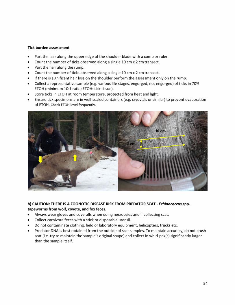
54

Tick burden assessment

• Part the hair along the upper edge of the shoulder blade with a comb or ruler. • Count the number of ticks observed along a single 10 cm x 2 cm transect. • Part the hair along the rump. • Count the number of ticks observed along a single 10 cm x 2 cm transect. • If there is significant hair loss on the shoulder perform the assessment only on the rump. • Collect a representative sample (e.g. various life stages, engorged, not engorged) of ticks in 70%

ETOH (minimum 10:1 ratio; ETOH: tick tissue). • Store ticks in ETOH at room temperature, protected from heat and light. • Ensure tick specimens are in well-sealed containers (e.g. cryovials or similar) to prevent evaporation

of ETOH. Check ETOH level frequently.

h) CAUTION: THERE IS A ZOONOTIC DISEASE RISK FROM PREDATOR SCAT - Echinococcus spp. tapeworms from wolf, coyote, and fox feces. • Always wear gloves and coveralls when doing necropsies and if collecting scat. • Collect carnivore feces with a stick or disposable utensil. • Do not contaminate clothing, field or laboratory equipment, helicopters, trucks etc. • Predator DNA is best obtained from the outside of scat samples. To maintain accuracy, do not crush

scat (i.e. try to maintain the sample’s original shape) and collect in whirl-pak(s) significantly larger than the sample itself.

10 cm

2 cm

55

i) PREDATOR DNA SWAB PROTOCOL

This protocol can be used when the predator species is unclear (i.e. predator hair and/or scat were not available to collect for DNA analysis). Equipment needed for double swab protocol: • Sharp knife and scalpel (with multiple, disposable blades) or disposable scalpels • Nitrile gloves • Sterile swabs - successful identification may be decreased depending on type of swab used. Prefer

individually packaged, fine tipped, cotton or poly swabs with plastic handle. • Paper envelopes • Whirl-paks • Silica desiccant • Sharpie • Stapler and staples • Small ethanol tubes for swab collection • Large ethanol tube for sterilizing knife • Kleenex/paper towel • Lighter • ** 95% ETOH is recommended as the best wetting agent for collecting swabs. Other wetting agents

(i.e. denatured alcohol, isopropyl alcohol) or sterile water can be used if 95% ETOH is not available however, there is potential for decreased success.

If carcass present: • Put on new nitrile gloves. • Carefully examine the carcass for killing wounds as identified by the presence of haemorrhage. • Take pictures of the wound (wide angle and close-up perspectives) without disturbing the wound

site. • Dip swab in the SMALL ethanol tube. • Swab wound (~10 seconds). • Place swab in non-Manila envelope and snap off shaft. • Staple envelope shut and label envelope with Wildlife Health ID and swab number using a sharpie

(e.g. xx-xxxx - 1A). • Place envelope in a whirl-pak with silica desiccant. • Fill out Predator Identification Data Form. Attach a copy of this form to the Caribou Mortality Site

Data Form • Repeat process on the same wound with a second swab (Identified as xx-xxxx - 1B) • Change gloves. • Identify other killing wounds or feeding wounds defined below (Identified as xx-xxxx - 2A, xx-xxxx - 2B,

etc.) and repeat the double swab process. If only bones and/or collar present: • Perform the double swab procedure on any remains (including the collar) that appear to have been

chewed on by predators.

56

Considerations: Avoid cross-contaminating wounds • Small amounts of DNA can easily be transferred between wounds. • Do not touch multiple wounds with the same gloves during wound identification. Identification of wounds • Carefully skin the animal trying to preserve puncture marks and determining areas of hemorrhage. • Sterilize knife after examining each wound - wipe knife with new Kleenex or paper towel - dip knife

blade in the LARGE ethanol filled tube, carefully, burn ethanol off blade using lighter. Bite description • Killing wound is a wound that caused death or that occurred before death as indicated by

hemorrhage. • Feeding wound is any other wound on a carcass such as bites or chewing with no hemorrhaging or

an area of the carcass that has been consumed. Swabbing Technique • AVOID DRENCHING THE SWAB IN BLOOD. • For killing wound - swab entire area around puncture wounds. • For feeding wound - concentrate swabbing on areas that appear to have been bitten or chewed.

Puncture Wounds

57

Predator Identification Data Form *Attach Copy to Moose Mortality Site Data Form*

Date (DD/MM/YYYY): ____________ Summary: Predator species 1: ____________ species 2: _____________ species 3: _____________ Unknown WLH ID (for the mortality): ____________________ Swab No. 1

Wound type (Circle) Killing

Feeding Other

_____________________

Wound Location and Description

Pictures

Check boxes as swabs are completed.

A B

Swab No. 2 Wound type (Circle)

Kill Feed Other

_____________________

Wound Location and Description

Pictures

Check boxes as swabs are completed.

A B

Swab No. 3 Wound type (Circle)

Kill Feed Other

_____________________

Wound Location and Description

Pictures

Check boxes as swabs are completed.

A B

Swab No. 4 Wound type (Circle)

Kill Feed Other

_____________________

Wound Location and Description

Pictures

Check boxes as swabs are completed.

A B

58

THE MORTALITY INVESTIGATION FORM AND ALL SAMPLES, WITH THE EXCEPTION OF THOSE IDENTIFIED FOR PRINCE GEORGE, MUST BE RETURNED TO:

Wildlife Health Program Attention: Ministry of Forests, Lands, Natural Resource Operations and Rural Development 2080 Labieux Road Nanaimo BC, V9T 6J9 Phone Numbers: Biologist: (xxx) xxx-xxxx Lab: (xxx) xxx-xxxx Shipping: • Frozen samples MUST remain frozen during transport or their use is compromised. • Appropriate insulated shipping containers and icepacks and can be purchased at low cost from

ULINE.ca or contact the Wildlife Health Program. • Formalin/fixed samples must be shipped separately from frozen samples. If tissues are

appropriately trimmed and have been fixed for > 36 hours, excess formalin can be drained off prior to shipping (leave samples covered by a piece of paper towel wetted with a small amount of formalin).

• When shipping tissue samples in formalin ensure they are in leak-proof, puncture-proof containers and double bagged with ample absorbent material (paper towel etc.) in case of leaks.

• Please notify the Wildlife Health Lab in Nanaimo BEFORE samples are shipped • Try to ship samples on Monday or Tuesday, never past Wednesday.