Determination of water quality parameters in Indian …...Determination of water quality parameters...

Determination of water quality parameters in Indian ponds

using remote sensing methods

Diploma thesis of

Christian Gemperli

Department of Geography, University of ZurichSupervised by Prof. Dr. K.I. Itten

Assisted by Dr. M. Kneubuehler (RSL) & Dr. R. Zah (EMPA)

Zurich, 01.06.2004

ACKNOWLEDGMENTS

Many persons contributed to the success of this thesis. I would like to thank everybody who sup-ported me during this time. Special acknowledgement deserve

• Prof. Dr. K. I. Itten for his interest and the perusal of my manuscript,

• Mathias Kneubuehler and Rainer Zah for the support and advices,

• M. Schaepman for the interest and support in the initial phase,

• the West Bengal Jute Project for the financial and logistical support,

• Dominik Noger for the advices concerning sampling procedure and measurements,

• Daniel Schlaepfer for the valuable advices regarding data processing and statistics,

• the staff of Bidhan Chandra Krishi Viswavidyalaya University, Mohanpur, for the coop-eration & infrastructure. Special thank goes to Prof. Dr. Hussein & Dr. Saha,

• the Spektrolab Team for the patience to answer my questions,

• Fieldwork Team for the cooperation & good time in India,

• Mr. Uehlinger (EAWAG) for the contribution to the technical infrastructure,

• Angela for the corrections,

• Sibylle for the patience,

• and finally my parents who enabled and supported my studies.

Zurich, May 2004 Christian Gemperli

ABSTRACT

In this thesis, the potential of existing algorithms and space borne imaging spectrometers for mon-itoring water quality were evaluated. In addition, the general state and the trophic conditions ofthe studied water bodies were assessed.

The concept of eutrophication was used to describe water quality, using chlorophyll as an indica-tor for the presence of algae in the water. Among the several concepts of eutrophication, theTrophic State Index of Carlson was chosen to define the trophic state of the water bodies.

Five small domestic ponds and one bayou of the Ganga river near the town of Kalyani, State ofWest Bengal, India, were selected as test-sites. During a field campaign in May 2003, reflectancespectra were measured 1m above the water surface using a handheld spectroradiometer. Concen-tration of TCHL and other limnological standard parameters such as Secchi Disk Depth, Nutrientcontent TOC and DOC were determined using laboratory analysis and a colorimetric testkit.

A comparison of several existing semi-empirical algorithms to determine chlorophyll content wasmade by applying them on the spectra and chlorophyll measurements collected in-situ. Simplereflectance band ratio and Continuum Interpolated Band Ratio (CIBR) were tested at severalwavelengths. Three tested algorithms rely on the reflectance peak at 700 nm whose shape andposition depend strongly upon chlorophyll concentration. The area and magnitude of the peakabove a baseline as well as the position of the peak show a linear relationship to chlorophyll-a con-centration from laboratory spectrophotometric measurements.

The algorithms were further applied onto spectra convolved to the bands of the hyperspectral sen-sors APEX, HyMap and Hyperion. A comparison of the spectral characteristics of the chosen sen-sors was made.

The domestic ponds showed extremely high chlorophyll concentrations around 300 µg/l and verylow Secchi Disk Depths around 0.1m indicating a hypertrophic situation. On the other hand, thenutrient concentrations were surprisingly low. The bajou showed almost no chlorophyll concen-trations, as well as low nutrient concentrations and higher Secchi Disk Depths.

All algorithms proved to be of value. Best results were obtained by using the algorithms Magni-tude above a Baseline and CIBR, with yielded around 0.97 and mean deviations around 20 µg/l. Given the large range of CHL concentrations, these results can be seen as very satisfactorily.However, certain presumptions had to be made and there still remain limitations concerning theused input data. Therefore, the results have to be treated with a certain caution.

The differences of the outcome of the sensors were small, but the results indicate that an interme-diate band width of around 10 nm seems appropriate. All sensors showed an adequate band posi-tioning for the algorithms based on the peak near 700 nm. Using simple band ratios and CIBR,APEX and Hyperion perform better than HyMap.

R2

ZUSAMMENFASSUNG

In dieser Diplomarbeit wurde das Potential von existierenden Algorithmen und Sensoren zumMonitoring von Wasserqualität evaluiert.

Das Konzept der Eutrophierung wurde herangezogen, um die Qualität des Wassers zu be-schreiben, wobei Chlorophyll als Indikator für den Algenwuchs diente. Mittels dem Trophic StateIndex (TSI) von Carlson wurde der trophische Status der Teiche bestimmt.

Das Untersuchungsgebiet befindet sich in der Nähe der Kleinstadt Kalyani in West Bengalen,Indien. Während der Feldarbeit im Mai 2003 wurden in fünf kleinen Teichen anthropogenen Urs-prungs und einem Altarm des heiligen Flusses Ganges Messungen vorgenommen. Die spektraleReflektanz des Wassers wurde 1 m über der Wasseroberfläche mittels einem tragbaren Spektro-radiometer gemessen. Die Konzentration von Chlorophyll und anderen limnologischen Standard-parametern wie Nährstoffgehalt, TOC und DOC, wurden mittels Laboranalysen und einem kolo-rimetrischen Schnelltestkit bestimmt. Zusätzlich wurden Tiefe, Secchi Disk Tiefe und Temperaturgemessen.

Verschiedene semi-empirischen Algorithmen zur Bestimmung des Chlorophyllgehalts wurdenmiteinander verglichen, indem sie auf die in-situ gesammelten Spektraldaten und Chlorophyll-messungen angewendet wurden. Einfache Band Ratio und Continuum Interpolated Band Ratio(CIBR) wurden bei verschiedenen Wellenlängen getestet. Drei weitere angewendete Algorithmenbasieren auf dem Reflektanzmaximum bei 700 nm, dessen Form und Position stark von der Chlo-rophyllkonzentration abhängt. Die Fläche und die Magnitude des Peaks über einer Normal-isierungslinie, wie auch die Position des Peaks auf der Wellenlängen-Achse, zeigen eine lineareBeziehung zu dem im Labor bestimmten Chlorophyllgehalt.

Weiter wurden die Algorithmen auf Spektren angewendet, die auf die Bänder von drei aus-gewählten hyperspektralen Sensoren (Hyperion, HyMap und APEX) gefaltet wurden. Dadurchkonnten die ausgewählten Sensoren miteinander verglichen werden.

Die kleinen, anthropogen entstandenen Teiche zeigten extrem hohe Chlorophyllgehalte um 300µg/l und Secchi Disk Tiefen von weniger als 0.1m, was auf eine hypertrophische Situation hin-deutete. Dennoch waren aber die gemessenen Nährstoffkonzentrationen überraschenderweise rel-ativ klein. Im Altarm des Ganges konnte kein Chlorophyll nachgewiesen werden. Die Nährst-offkonzentrationen waren auch hier sehr klein, die Secchi Disk Tiefe grösser.

Alle Algorithmen bewährten sich. Die besten Resultate wurden mit der Magnitude des 700 nmPeak und CIBR erzielt, mit von 0.97 und mittleren Abweichungen von rund 20 µg/l. In Hin-sicht auf den sehr grossen Range von Chlorophyllgehalten innerhalb des Datensatzes, kann diesesResultat als sehr befriedigend bezeichnet werden. Es mussten jedoch Annahmen getroffen werdenund weiterhin bestehen einige Unsicherheiten bezüglich der verwendeten Datensätze. Deshalbsind die erzielten Resultate mit gewisser Vorsicht zu geniessen.

R2

Die Unterschiede zwischen den einzelnen Sensoren waren sehr gering, die Resultate deutenjedoch an, dass für die verwendeten Algorithmen eine Bandbreite von etwa 10 nm ideal ist. DieBänder aller Sensoren sind für die auf dem 700 nm Peak basierenden Algorithmen geeignet. Beider Anwendung von einfachen Band Ratios und CIBR zeigten APEX und Hyperion bessereResultate als HyMap.

TABLE OF CONTENTS

TABLE OF CONTENTS .........................................................................................1

LIST OF FIGURES .................................................................................................. 4

LIST OF TABLES.................................................................................................... 5

ABBREVIATIONS................................................................................................... 6

1. INTRODUCTION ......................................................................................... 71.1 Background ..................................................................................................................................... 7

1.2 Scope & aims ................................................................................................................................... 7

1.3 Outline.............................................................................................................................................. 8

2. THEORY ....................................................................................................... 92.1 Water quality................................................................................................................................... 9

2.1.1 Overview.................................................................................................................................................... 9

2.1.2 Eutrophication .......................................................................................................................................... 9

2.1.2.1 Trophic State Index (TSI) by Carlson [5] ................................................................................................................ 10

2.2 Water Optics.................................................................................................................................. 11

2.2.1 Inherent optical properties .................................................................................................................... 11

2.2.2 Apparent optical properties .................................................................................................................. 12

2.2.3 Interaction between Inherent and Apparent Optical Properties....................................................... 13

2.2.4 Optically active substances .................................................................................................................... 13

2.2.4.1 Water ........................................................................................................................................................................ 142.2.4.2 Yellow substances (Gelbstoff) ................................................................................................................................. 142.2.4.3 Seston ....................................................................................................................................................................... 14

2.2.5 Influence of the constituents onto the reflectance spectrum .............................................................. 15

2.3 Remote sensing of water quality parameters ............................................................................. 16

2.3.1 Approaches.............................................................................................................................................. 16

2.3.2 Sensors..................................................................................................................................................... 17

2.3.2.1 Selection of different sensors for convolution of spectral bands ............................................................................. 18

3. DATA ACQUISITION ............................................................................... 213.1 Study area ...................................................................................................................................... 21

3.2 Selection of water bodies .............................................................................................................. 22

3.3 Data ................................................................................................................................................ 23

3.3.1 Spectral data ........................................................................................................................................... 23

3.3.2 Water constituents data ......................................................................................................................... 24

3.3.2.1 Sampling scheme...................................................................................................................................................... 253.3.2.2 Determination methods ............................................................................................................................................ 253.3.2.3 Quality remarks concerning chlorophyll in-situ data............................................................................................... 26

4. SPECTRAL DATA PROCESSING & ANALYSIS................................. 274.1 Pre-processing ............................................................................................................................... 27

4.1.1 Correction of sunglint effects ................................................................................................................ 28

4.1.2 Convolution............................................................................................................................................. 29

1

4.2 Description of the reflectance curve............................................................................................ 29

5. LIMNOLOGICAL ASSESSMENT........................................................... 315.1 General description of the water bodies ..................................................................................... 31

5.2 Analysis of retrieved limnological data....................................................................................... 32

5.2.1 Chlorophyll and assumed algae composition....................................................................................... 32

5.2.2 Nutrient content...................................................................................................................................... 34

5.2.3 Organic Carbon...................................................................................................................................... 34

5.2.4 Secchi disk depth .................................................................................................................................... 35

5.2.5 Other limnological parameters ............................................................................................................. 35

5.2.5.1 pH............................................................................................................................................................................. 355.2.5.2 Total hardness .......................................................................................................................................................... 355.2.5.3 Heavy metals ............................................................................................................................................................ 35

5.3 Trophic state.................................................................................................................................. 36

5.4 Conclusions.................................................................................................................................... 37

6. METHODOLOGY OF PARAMETER RETRIEVAL............................ 386.1 Methods used in this study........................................................................................................... 38

6.1.1 Selection of appropriate methods ......................................................................................................... 38

6.1.2 Chlorophyll determination algorithms................................................................................................. 38

6.1.2.1 Band ratio ................................................................................................................................................................. 386.1.2.2 Continuum Interpolated Band ratio (CIBR)............................................................................................................. 396.1.2.3 Area above baseline ................................................................................................................................................. 406.1.2.4 Peak Magnitude above baseline ............................................................................................................................... 416.1.2.5 Position of the Peak near 700 nm............................................................................................................................. 42

6.1.3 Statistical methods.................................................................................................................................. 43

6.1.3.1 Regression Analysis ................................................................................................................................................. 43

7. RESULTS OF PARAMETER DETERMINATION ............................... 457.1 Setup............................................................................................................................................... 45

7.2 Modelling using Fieldspec FR PRO bands ................................................................................. 46

7.2.1 Simple band ratios.................................................................................................................................. 46

7.2.2 CIBR ........................................................................................................................................................ 47

7.2.3 Area above base line............................................................................................................................... 48

7.2.4 Peak Magnitude above a baseline ......................................................................................................... 49

7.2.5 Position of peak near 700 nm ................................................................................................................ 49

7.3 Modeling using convolved spectra............................................................................................... 50

8. DISCUSSION............................................................................................... 528.1 Interpretation of results of spectral modelling........................................................................... 52

8.2 Quality assessment and source of errors .................................................................................... 54

9. CONCLUSIONS.......................................................................................... 559.1 Future Improvements................................................................................................................... 55

9.1.1 Sampling Procedure ............................................................................................................................... 55

9.1.2 Data Processing....................................................................................................................................... 55

9.2 Defiances for a future monitoring system................................................................................... 56

9.3 Outlook........................................................................................................................................... 56

2

REFERENCES............................................................................................ 58

APPENDIX ................................................................................................... 62A. Additional Tables and Figures..................................................................................................... 62

Limnological classification schemes ............................................................................................................... 62

Sampling scheme and parameter determination........................................................................................... 63

Results of limnological measurements............................................................................................................ 64

B. Used methods for parameter extraction ..................................................................................... 65

B.I Chlorophyll determination in water samples by Annon`s method.................................................... 65

B.II Dissolved organic carbon by dichromate oxidation method of Vance .............................................. 66

B.III Total organic carbon by Nelson Somers method................................................................................. 67

C. Description of additional limnological parameters.................................................................... 68

D. Field sheets..................................................................................................................................... 71

3

4

LIST OF FIGURES

Fig. 2.1: Absorption coefficients of active constituents. ................................................. 14

Fig. 2.2: Scattering coefficients of active constituents. ................................................... 14

Fig. 2.3: Absorbance peak of phycocyanin on spectrum of P2. ...................................... 16

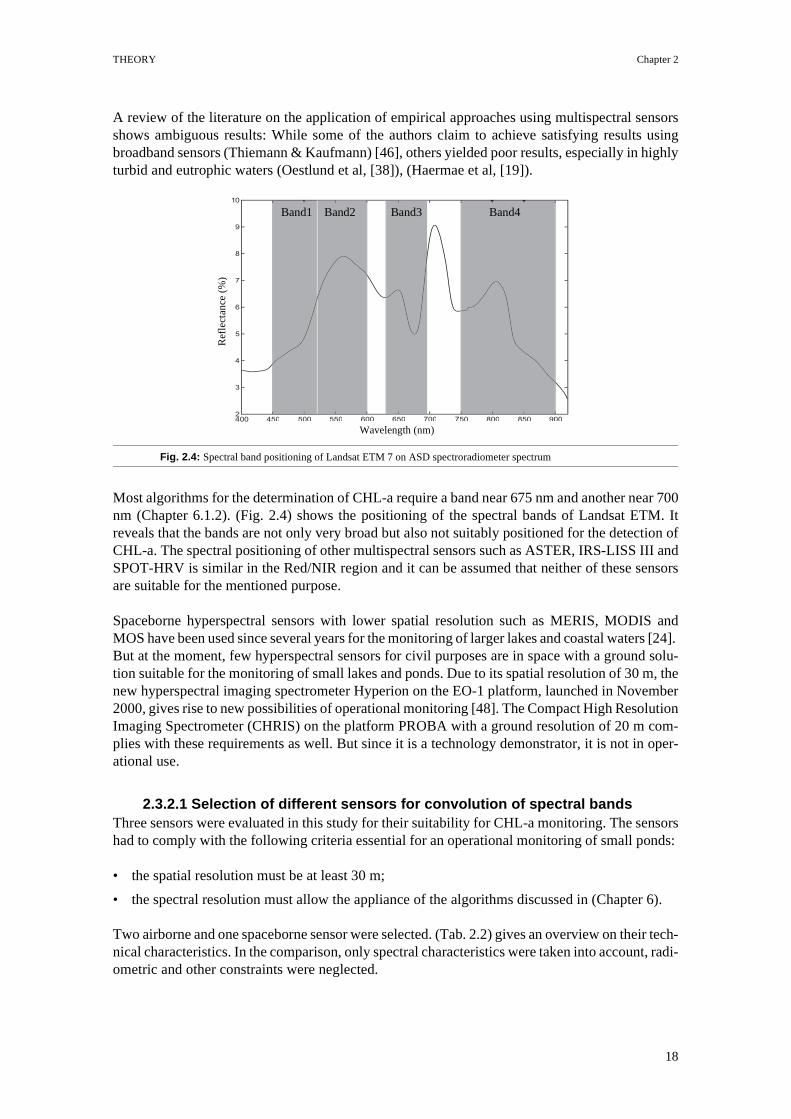
Fig. 2.4: Band positioning of Landsat ETM 7 on ASD spectroradiometer spectrum ..... 18

Fig. 3.1: Map of West Bengal District ............................................................................ 21

Fig. 3.2: Landsat ETM panchromatic image 22.04.2002 ................................................ 22

Fig. 3.3: Selected water bodies and covered transects .................................................... 23

Fig. 4.1: Averaged spectra of each water body ............................................................... 27

Fig. 4.2: Effect of sunglint on reflectance spectra........................................................... 28

Fig. 4.3: FWHM defined as spectral resolution .............................................................. 29

Fig. 5.1: From left to right: P1, P2, P5 and P6 ................................................................ 31

Fig. 5.2: Dominant phytoplankton in Indian reservoirs .................................................. 33

Fig. 6.1: Band ratio algorithm ......................................................................................... 39

Fig. 6.2: Continuum Interpolated Band ratio (CIBR)...................................................... 40

Fig. 6.3: Base line algorithm ........................................................................................... 41

Fig. 6.4: Peak Magnitude above Baseline algorithm by Gitelson ................................... 42

Fig. 6.5: Peak Position algorithm by Gitelson................................................................. 42

Fig. 7.1: Linear (left) and logarithmic (right) curve fit between CHL in-situ data and the normalized spectra ............................................................................................ 46

Fig. 7.2: Linear curve fit for CIBR [651/675/713] (left) and its band positions on the reflectance spectra............................................................................................. 48

Fig. 7.3: The range of the position of the peaks on the wavelength axis ........................ 49

Fig. 7.4: Spectra convolved to the bands of the chosen sensors...................................... 51

Fig. 8.1: Necessary bands for used algorithms on band positions of chosen sensors ..... 53

5

LIST OF TABLES

Tab. 2.1: Comparison of TSI to Water Quality Parameters and Lake Productivity......... 11

Tab. 2.2: Characteristics of chosen sensors...................................................................... 19

Tab. 3.1: Recorded spectra ............................................................................................... 24

Tab. 3.2: Determined limnological parameters ................................................................ 24

Tab. 3.3: TCHL values for data set1 & 2 ......................................................................... 26

Tab. 5.1: Characteristics of the selected ponds ................................................................ 32

Tab. 5.2: Correlation between several limnological parameters ...................................... 35

Tab. 5.3: Calculated TSI values ....................................................................................... 36

Tab. 7.1: Results of ratios: linear fit; raw data ................................................................. 46

Tab. 7.2: Results for ratios: linear fit; normalized at 900nm ........................................... 46

Tab. 7.3: Results for ratios: logarithmic fit. ..................................................................... 47

Tab. 7.4: Statistical coefficients for CIBR algorithm applied on Fieldspec FR PRO...... 47

Tab. 7.5: Results for area above baseline algorithm ........................................................ 48

Tab. 7.6: Statistical coefficients for peak magnitude above a baseline............................ 49

Tab. 7.7: Statistical coefficients for peak position ........................................................... 49

Tab. 7.8: Results of simple band ratio; logarithmic fit..................................................... 50

Tab. 7.9: Results of CIBR; linear fit ................................................................................ 50

Tab. 7.10: Results of area a. baseline for convolved spectra ............................................. 50

Tab. 7.11: Results of magnitude a. baseline for convolved spectra ................................... 50

Tab. 8.1: Position of needed bands and availability of the sensors.................................. 52

Tab. A.1: Classification scheme according to frequency of overturn by WHO ............... 62

Tab. A.2: Characteristics of trophic states according Carlson. ......................................... 62

Tab. A.3: Determined parameters for each sampling location.......................................... 63

Tab. A.4: Measuring range and estimated error of colorimetric method (Aquanal)......... 63

Tab. A.5: Results of limnological parameters determined in India .................................. 64

Tab. A.6: Results of ICP-OES determination at EMPA ................................................... 64

6

ABBREVIATIONS

Spectrometric abbreviations

a absorption coefficient b scattering coefficient c : beam attenuation coefficient

: Remote Sensing reflectance [%]Sub-surface irradiance reflectance [%]Water-leaving radiance Downwelling irradiance

nm nanometerwvl wavelength

Statistical abbreviations

per cent Mean Deviationabsolute Mean Deviation

Correlation CoefficientStd error Standard error

Limnological abbreviations

SDD Secchi Disk DepthCHL-a Chlorophyll aTCHL Total chlorophyllTOC Total Organic Carbon DOC Dissolved Organic CarbonZN ZincAS ArsenicTh Total hardnessInteg. SDD Mixed sample from the water column between 0 m and SDD.ICP-OES Inductively Coupled Plasma Optical Emission Spectroscopy

n/d not determinedbdl below detection limit

Units

µg/L micrograms per Liter or ppb (parts per billion).mg/L milligrams per Liter or ppm (parts per million).

m 1–[ ]m 1–[ ]

m 1–[ ]

RR

R 0–( )LW 0( ) Wm 2– nm 1– sr 1–[ ]ED 0( ) Wm 2– nm 1–[ ]

MDℵ

MDa

R2

Chapter 1 INTRODUCTION

1 INTRODUCTION

1.1 Background

The West Bengal Jute Project lead by IBF AG, Sustena IG and EMPA deals with the sustainablemanagement of fiber crops in West-Bengal over the whole value chain.

In jute production, retting is a very important step to the final quality of the fibre. After harvesting,the crops are immersed in rivers, canals, ponds and ditches and left there for about 2 to 3 weeksbefore the fibres can be extracted from the plant. An important condition for good retting is thequality of the used water, meaning, the water should be clear and oxygen-rich. Therefore, rettingin rivers is preferred to retting in ponds and other water bodies without outlet. At the same time, retting influences the water quality. It can be assumed that the input of largeamounts of organic material and nutrients affects the water quality at least temporarily.

Classical techniques for determining indicators of water quality involve in-situ measurements andlaboratory analysis. Although these approaches give accurate results, they are time-consuming,expensive and do not give a spatial view on the needed variables as they represent point-in-timemeasurements. Remote sensing of water quality parameters has the potential to determine theseparameters at relatively low costs on a frequent basis offering a spatial view on the parameters.These advantages are especially interesting in remote areas of little or restricted access and withfew analytical resources such as laboratories and trained staff.

To get an overview of the current state of the various ponds within the wide and sometimes diffi-cultly accessible terrain of West Bengal, India, remote sensing techniques seem to be appropriatedue to the reasons mentioned above.

1.2 Scope & aims

The scope of this work is to investigate the potential of algorithms in monitoring water qualityparameters in West Bengal ponds. The concept of eutrophication was chosen to describe waterquality, using chlorophyll as indicator for the presence of algae in the water. A semi-empiricalapproach was used to determine the parameter. The algorithms chosen from the literature had toperform well in other studies on water bodies with comparable limnological characteristics.The aims of the study are as follows

• to asses the trophic state of the ponds,

• to evaluate semi-empirical algorithms for determining chlorophyll-a content using spectral reflectance data collected with a handheld field-spectroradiometer,

• to apply these algorithms to the spectra convolved to the bands of selected sensors,

• and to evaluate the most suitable sensors and applied algorithms for determining chlorophyll-a content in the study area.

7

INTRODUCTION Chapter 1

1.3 Outline

Chapter 2 deals with the theoretical background of the field of study. It gives a description of theconcept of eutrophication and of the optical properties of water and its constituents, such as phy-toplankton, total suspended solids and colored dissolved organic matter. An overview of theapproaches used for the determination of these constituents and the resulting advantages and dis-advantages is presented as well as a short description of the technical characteristics of the sensors,of which the potential was investigated.

Chapter 3 gives a detailed description of the campaign, which was carried out to gather spectraland limnolocigal data of the ponds. It describes the study area, where the field measurements tookplace, and it shows the schemes which were used in the sampling process and the methods toextract the desired parameters. A list of all gathered data and quality remarks is presented.

Chapter 4 describes the process of data pre-processing and explains briefly the concept of convo-lution of spectral bands. The spectral reflectance curves of the water bodies are analyzed and dis-cussed briefly.

In Chapter 5 the results of the limnological assessment are discussed. A description of the limno-logical characteristics of the ponds are given and conclusions about its trophic state are drawn.

Chapter 6 deals with the methods used for the retrieval of chlorophyll-a of the reflectance spectraand the statistical parameters having used to quantify the results.

In Chapter 7, the results of the different methods for the determination of the parameters are pre-sented for (1) the spectra measured with the handheld spectroradiometer, and (2) for the men-tioned spectra which were convoluted to the spectral bands of the sensors described in Chapter 2.

Chapter 8 discusses the results presented in Chapter 7. It shows the limitations and quality aspectsof the data, which were used in the modeling process and gives explanations for the results.

In Chapter 9, improvements for the future are proposed and general defiances for a water qualitymonitoring system based on Remote Sensing in West Bengal are considered.

8

Chapter 2 THEORY

2 THEORY

2.1 Water quality

2.1.1 Overview

There is no single definition of water quality, as it depends on the respective processes and on theintended use of the water. In this work the focus is laid on the process of eutrophication. Trophicstate is an absolute scale that describes the biological condition of a water body and does not implya normative statement per se. It has to be stressed that trophic state is not the same thing as waterquality but trophic state certainly is one aspect of water quality.To give a general impression of the state of the ponds, some additional limnological standard vari-ables determined during the campaign will be discussed in Chapter 4.

2.1.2 Eutrophication

The term ‘eutrophication’ means nutrient enrichment of lakes and describes the processes in watercaused through over-enrichment by nutrients. Too much nutrient input causes a chain of eventsthat may have undesirable effects on lakes, e.g. growth of algae and macrophytes. The enhancedrates of decomposition and attendant consumption of oxygen lead finally to oxygen depletion inthe hypolimnion, decreasing the number of species. Eutrophication can occur under natural con-ditions, but often the process is induced by anthropological factors, such as fertilizers and sewage[5]. Organic matter introduced to surface waters (e.g. jute), leads to enhanced rates of decompo-sition and attendant consumption of oxygen.

Numerous definitions of trophic state exist in the literature and there have been several attemptsto classify lakes according to their trophic condition. They vary in the indices they use to assessthe trophic state and in the classification schemes they use to separate lakes in different classes.Generally, one can distinguish between classification approaches which are based on productivityand biomass (e.g. chlorophyll-a concentration) or definitions based on the factors determining thisproduction (e.g. phosphorus loadings). Other approaches focus on the effects that are caused bythe process of eutrophication (e.g. hypolimnetic oxygen depletion, Secchi Disk Depth). Some con-temporary classification schemes use only a single variable to define the trophic state of lakes.This use of a single variable simplifies the classification procedure considerably because only onevariable has to be measured. At the same time, this approach reduces the concept of eutrophica-tion, which rather describes a process, than a state or class, significantly.

The early approach of Naumann (1919) divided the lakes into several classes based on biomassproduction, e.g oligotrophic lakes were low in production, eutrophic lakes were very productive.He then related the classes to several indicators, such as humic content, nitrogen and phosphorus,iron, pH, oxygen, and carbon dioxide [45].

9

THEORY Chapter 2

Hutchinson (1969) and Odum (1969) emphasized the importance of the watershed to define thetrophic state by the loading of nutrients to the lake. In this context, trophic state was a descriptionof the potential for a lake to respond to nutrient loading rather than a description of the response.A eutrophic system would be a system in which the total potential concentration of nutrients washigh, whether or not there was a correspondingly high algal or macrophyte density [5].

The OECD index of Vollenweider and Kerekes (1980) is a classification system based on theprobability that a lake or reservoir will have a given trophic state. The index was generated by ask-ing a group of scientists their opinion as to what was the average value of the indicator (e.g. Totalphosphorus) for each trophic class. Therefore, lakes of the same concentrations may be in morethan one trophic class. The assumed advantage of the probabilistic approach is that responses to agiven variable will vary from lake to lake and therefore prediction of its trophic state is best statedin probabilistic terms [45].

Carlson (1977) suggested returning to the initial principles of trophic state: a quantifiable conceptbased on biomass. He used Naumanns (1929) original idea of classification according to plant bio-mass. But instead of the distinct typological classes, Carlson assumed algal biomass to be from acontinuous range of values. This approach will be used in this work as it is relatively simple to useand only requires a minimum of data [51].

2.1.2.1 Trophic State Index (TSI) by Carlson [5]According Carlson, trophic state is defined as the total weight of living biological material (bio-mass) in a water body at a specific location and time. It is estimated independently by three vari-ables: chlorophyll-a pigments, Secchi depth, and total phosphorus (TP).

For each variable the Trophic State Index (TSI) is calculated by a separate equation. The advan-tage of this index is that a similar TSI value can be obtained from each of the three variables.Although these three variables should co-vary, they should not be averaged, because neither trans-parency nor TP are independent estimators of trophic state. For the purpose of classification, pri-ority is given to chlorophyll because this variable is the most accurate of the three at predictingalgal biomass. Secchi depth and TP should be used as a surrogate and not as a co-variate of chlo-rophyll.

The basic Secchi Disk index (Equation 2.1) was constructed from a doubling and halving of Sec-chi disk transparency, where the base index value is a Secchi depth of 1 m, the logarithm of whichis 0 (Tab. 2.1).

, (2.1)

The index uses relationships between trophic variables to produce equations that allow the indexto be calculated from variables other than Secchi depth. The indices for the chlorophyll and TPEquation 2.2 are obtained in a similar manner, but instead of a Secchi depth value in the numera-tor, the empirical relationship between chlorophyll or TP and Secchi depth is given.

, (2.2)

TSI SD( ) 10 6 SDln2ln

-------------–=

TSI CHL( ) 10 6 2.04 0.68 CHLln–2ln

---------------------------------------------–=

10

Chapter 2 THEORY

, (2.3)

where TP and CHL-a are expressed in µg/l. SD is expressed in meters. TSI is unitless.

The range of the index (Tab. 2.1) is from approximately zero to 100, although the index theoreti-cally has no lower or upper bounds. Unlike Naumann’s typological classification of trophic state,the index reflects a continuum of states and there are no lake “types”.

2.2 Water Optics

The optical properties of water are often divided into the Inherent Optical Properties (IOP) and theApparent Optical Properties (AOP), which are defined by the first mentioned.

2.2.1 Inherent optical properties

The Inherent Optical Properties are the properties of the medium itself (i.e., water plus constitu-ents). They depend only upon the medium. Thus, regardless of the ambient light field the IOP aremeasured by active optical instruments. The main active constituents which will be described in(Chapter 2.2.4) are aquatic humus, phytoplankton and tripton.

There are two main optical processes, absorption and elastic scattering, quantified by the absorp-tion coefficient a and the volume-scattering function β, respectively. Other inherent optical prop-erties, which can be obtained from the absorption coefficient and the volume-scattering function,are the scattering coefficient b and the beam attenuation coefficient c [8].

The absorption coefficient is defined as the sum of the individual absorption coefficients of thesewater constituents (Beers law). Assuming a linear relationship between absorption and concentra-tion, it is given as

Trophic state TSI Secchi Disk (m) Total Phosphorus (µg/L) Chlorophyll-a (µg/L)

Oligotrophic 0 64 0.75 0.04

10 32 1.50 0.12

20 16 3 0.34

30 8 6 0.94

Mesotrophic 40 4 12 2.60

50 2 24 6.40

Eutrophic 60 1 48 20

70 0.5 96 56

Hypereutrophic 80 0.25 192 154

90 0.12 384 427

100 0.06 768 1,183

Tab. 2.1: Comparison of Trophic State Index to Water Quality Parameters and Lake Productivity [5].

TSI TP( ) 10 6

48TP-------ln

2ln-------------–=

11

THEORY Chapter 2

, (2.1)

where is the absorption by pure water, by aquatic humus, by phytoplankton, by tripton and the corresponding concentration of the constituents.

As scattering is mainly caused by water, phytoplankton and tripton the scattering coefficient b canbe written as

, (2.2)

The beam attenuation coefficient, representing the total loss of light due to absorption and scatter-ing [7], is defined as

. (2.3)

2.2.2 Apparent optical properties

Apparent optical properties depend both on the medium and on the ambient light field. Therefore,in contrast to the IOP, they can only be determined in-situ. Commonly used apparent optical prop-erties are the radiance, irradiance, reflectance and the vertical-attenuation coefficient. Dekker [7]and Frauenhofer [8] give a detailed overview.

In remote sensing of water quality, the most important reflectance definitions are the sub-surfaceirradiance reflectance and the remote sensing reflectance.

For the remote sensing reflectance two different definitions exist. Sometimes, the radiance reflec-tance is referred to remote sensing reflectance which is given through

, (2.4)

where is the water-leaving radiance influenced by the active constituents. isthe downwelling irradiance.

If a white reflectance panel is used to ‘calibrate’ the sensor, a diffuse homogeneous mixture of allthe full sky and sun radiance reflects at nearly 100 percent up to the fiber-optic input. Therefore,the irradiance becomes

, (2.5)

leading to the bi-directional reflectance, which will be used in this work.

(2.6)

a total( ) C w( ) a× w( ) C ah( ) a× ah( ) C ph( ) a× ph( ) C t( ) a× t( )+ ++=

a w( ) a ah( ) a ph( )a t( ) C

b total( ) C w( ) b× w( ) C ph( ) b× ph( ) C t( ) b× t( )++=

c a b+=

RRLW 0( )ED 0( )-------------- sr 1–[ ]=

LW 0( ) ED 0( )

E λ( ) π L λ( )⋅=

RRLW 0( )LD 0( )-------------- sr 1–[ ]=

12

Chapter 2 THEORY

The sub-surface irradiance reflectance which is often used in analytical models has to be mea-sured below the water surface. It is defined as the ratio of the upwelling and the downwelling irra-diance [12].

. (2.7)

2.2.3 Interaction between Inherent and Apparent Optical Properties

Several models exist, which link the IOP to the AOP. Analytical and semi-analytical approachesuse them to relate the different measured IOP to the AOP obtained by remote sensing methods.An overview of models mainly for ocean water is given by Gordon & Morel [18] and extendedfor inland water by Kirk [26].

A commonly used model links to the backscattering and absorption coefficients with

, (2.8)

where and are the absorption and backscattering coefficients given by Equation 2.1 andEquation 2.2. defines the beam attenuation coefficient and is a coefficient dependent on solarzenith angle and the volume scattering function [7].

Monte Carlo simulations by Morel & Prieur [33] showed, that Equation 2.8 can be simplified to

, (2.9)

where is approximately 0.33 for smaller than 0.25 .

Two very simple conclusions can be drawn from Equation 2.8:

(1) The greater the backscattering, the more light is scattered up towards the water surface, thegreater the radiance reflectance.

(2) The greater the absorption, the greater the probability that a photon is absorbed prior to beingscattered upward, the lower the radiance reflectance [30].

2.2.4 Optically active substances

The main optically active constituents that influence the IOP are pure water, yellow substances,often referred to as Gelbstoff, and seston which can be further divided into tripton and phytoplank-ton.

2.2.4.1 WaterPure water does not absorb strongly in the blue-green region but increasingly at wavelengthsbeyond 550 nm. At 700 nm absorption increases exponentially with a peak at approximately 750nm. Scattering by water is inversely proportional to wavelength and causes its blue color.

R 0–( ) EW 0–( )ED 0–( )------------------=

R 0–( )

R 0–( ) r1bb

a bb+( )------------------- r1

bb

c----= =

a bb

c r1

R 0–( ) r1bb

a----=

r1bb

a---- m 1–

13

THEORY Chapter 2

2.2.4.2 Yellow substances (Gelbstoff)Yellow substances, in the literature also referred to as Gelbstoff, aquatic humus, humic acid or gil-vin, are decomposed organic substances originating from authochtonous production within thewater or from allochthonous sources from organic breakdown products on land. Yellow sub-stances mainly consist of dissolved organic carbon in form of dissolved fulvic and colloidal humicacids [7].Absorption of yellow substances decreases exponentially with increasing wavelength. In openoceanic waters, its absorption can be neglected at wavelengths beyond 625 nm [28]. However, in inland waters with high content of humus concentration it is not negligible: accordingto Dekker [7], yellow substances can make up to 30% of the absorption by pure water at 700 nmand influence total absorption up to wavelengths beyond of 720 nm. As in productive lakes anincrease in absorption of yellow substances tends to covary with an increase in lake trophic status[7]. Therefore, influence in the Indian ponds should be strong.The parameter is especially interesting for remote sensing, as it influences the determinability ofother substances, but it has hardly been determined successfully by means of remote sensing yet[24].

2.2.4.3 SestonSeston is the collective name for all particulate matter suspended in water which does not passthrough a filter of 0.45 µm [7]. It consists of live organic material (phytoplankton) and deadorganic (detrius) and inorganic matter. Tripton refers to the sum of all dead material, thus detriusand inorganic material1 [25].

TriptonAs stated above, tripton is the sum of dead organic and non-organic material suspended in water.Absorption properties are similar to those of aquatic humus. It shows an exponentially increasingslope in the blue region. With increasing wavelength, absorption decreases; it is almost not exis-tent in the red region [28]. It must be kept in mind, however, that the inorganic parts in high con-centration will have their own color and will influence the absorption properties independently ofthe other constituents [24].

1. Seston = phytoplankton + Tripton [dead organic (Detrius) + inorganic matter]

Fig. 2.1: Absorption coefficients of active constituents after [12]. Fig. 2.2: Scattering coefficients of active constituents after [12].

14

Chapter 2 THEORY

PhytoplanktonPhytoplankton refers to all phototrophic active organisms in water. Phytoplankton influences theoptical properties of the water by means of absorption and scattering. During absorption the pig-ments transform light (photons) into other forms of energy. The most relevant pigments for wateroptics are chlorophylls, phaeophytins, carotenoids and phycobiliproteins.

The group of chlorophylls is comprised of CHL-a, -b, -c1, -c2, and -d, which vary in their chem-ical structure. Unlike all other chlorophyll pigments, CHL-a can be found in all photosyntheticactive organisms. Therefore, it is the most important pigment serving as an indicator for the bio-logical activities in inland water. The absorption spectrum of phytoplankton is mainly dominatedby absorption of CHL-a; the influence of the accessory pigments -a and -b can be neglected in thered region of the spectrum. The absorption maxima of CHL-a can be found at 440 nm in the blueand at 675 nm in the red portion of the spectrum, whereby the position of the maxima can vary upto 5 nm. In the green region chlorophyll absorption is low which gives the pigment its character-istic color. Depending on the composition of algal species, the proportion of CHL-a to total chlo-rophyll (TCHL) varies. In the cyanophycea (blue-green algae), CHL-a occurs unaccompanied byother chlorophyll groups [24].

Pheophytin is a product of chl degradation. Its chemical structure and absorption properties arealmost identical to those of CHL-a.

Carotenoids occur much more often than chlorophylls, but their role in the photosynthetic processof algae is less crucial [24].

Red and blue algae contain phycobiliproteins, which absorb between 540 and 650 nm. The pig-ment phycocyanin, which occurs in cyanobacteria, belongs to this group and has its peak absorp-tion at 630 nm [7].

2.2.5 Influence of the constituents onto the reflectance spectrum

The range between 400- 500 nm is influenced by all optically active substances. Strong absorptionin the blue is shown by dissolved organic matter as well as by chlorophyll and carotenoids. Scat-tering by particulate matter is also strong. The reflectance minimum at 440 nm represents the firstCHL-a absorption peak and can be used for the estimation of CHL-a in ocean water (band ratio[440/550]). Due to the dominance of dissolved organic matter and particulate material in eutrophicwater bodies, absorption of pigments becomes masked in this region. Another trough caused byabsorption of carotenoids can be found at approximately 490 nm. As absorption of chlorophyll islow in the green region, algae-rich spectra show a peak in reflectance at around 550-570nm, whichis called the green peak.

The existence of blue-green algae in the water body is indicated by a trough in reflectance atapproximately 630 nm, the phycocyanin absorbtion peak (Fig. 2.3). Increasing content of phyco-cyanin leads to increase in depth of the trough and shifts the green peak towards shorter wave-lengths. Thus, in waters with blue-green algae, the green peak position depends on at least twofactors: carotenoid and phycocyanin concentrations [16].

15

THEORY Chapter 2

Fig. 2.3: Absorbance peak of phycocyanin on spectrum of P2.

The reflectance peak near 700 nm, which was described by Gitelson [13], lies in between tworeflectance minima. At lower wavelengths CHL-a has its peak absorption at 675 nm (Fig. 2.3). Atthis wavelength, absorption and scattering by cell walls are almost in equilibrium. Therefore,reflectance depends mainly on scattering of in-organic particulate matter. Beyond 750 nm, waterabsorbs increasingly and reflectance, depending mainly on both organic and in-organic suspendedmatter, is insensitive to algal pigments. The shape of the peak depends strongly on CHL-a con-centration. With increasing content, its magnitude increases and the peak shifts towards longerwavelengths.

There have been several attempts to explain the peak near 700 nm. It might be caused through:

(1) fluorescence of phytoplankton pigments (Morel and Prieur [33]), (Gordon [17]),

(2) anomalous scattering caused by the chlorophyll absorption peak at 675 nm (Morel and Prieur[33]) or

(3) a minimum on the combined absorption curve of water and algae for high chlorophyll values(Vasilkov & Kopelevich [52]).

[13]

2.3 Remote sensing of water quality parameters

2.3.1 Approaches

Since the late 1970’s, bio-optical algorithms were developed to determine water quality parame-ters. Initially, algorithms were developed for oceans, where optical properties are determinedsolely by phytoplankton and its breakdown products. A few spectral bands in the blue to greenspectral region are sufficient to determine CHL-a concentrations with adequate precision in theseoptically relatively simple waters known as Case 1 waters. In Case 2 waters (inland and coastalwaters), the optical properties are determined, additionally to phytoplankton, by a composite ofdissolved organic matter from terrestrial origin, dead particulate organic matter and particulate

400 450 500 550 600 650 700 750 800 8503

4

5

6

7

8

9

10

Wavelength (nm)

Ref

lect

ance

(%)

Phycocyanin absorption peakCHL-a absorption peaksCHL-b absorption peaks

O2Absorption

‘Peak near 700nm’

‘Green Peak’

16

Chapter 2 THEORY

inorganic matter. As the constituents are not statistically correlated, its determination is muchmore complex and less accurate. CHL-a algorithms developed for Case 1 waters are generally notapplicable to Case 2 waters as the blue-green region is often masked by Gelbstoff absorption.Therefore, they concentrate on the second absorption maximum of CHL-a in the red and nearinfrared region of the spectrum [8].

Morel & Gordon [17] distinguished three different approaches to estimate concentrations of waterconstituents, the empirical, the semi-empirical and the physical approach. The empirical approach seeks statistical relationships between spectral bands or band combina-tions and the measured water parameters without including knowledge about spectral characteris-tics of the constituents or any physical explanation of the relationship. With the semi-empirical method, physical and spectral knowledge (e.g. absorption features) areused to develop the algorithms, which are then correlated to the measured constituents. The sta-tistical coefficients are normally bound to the specific region and time of calibration. Analytical approaches derive the concentration of the constituents by modeling the way of thelight flux in the water and the atmosphere by using the Inherent and Apparent Optical Properties. The semi-analytical approach mentioned by Keller [24] uses simplified analytical models.

The advantage of the empirical approaches is its easy implementation as less mathematical skillsand computation time is required. On the other hand, the method is not applicable if the parameterhas a no distinctive absorption features as it is the case for Gelbstoff and to a certain extent forsuspended matter [24].The advantage of the analytical approach is that all constituents can be determined simulta-neously, if the inherent properties of the parameters are well known and large amounts of in-situdata are given. The approach is further applicable to various water types and is not bound to thetime the in-situ measurements were made [7].

The accuracy of the different approaches depends on the water type and is difficult to predict.Even if in recent years the development of analytical approaches has advanced, semi-empiricalmethods are still mostly used in this field [16],[46],[30],[29],[19].

2.3.2 Sensors

Until today, remote sensing of water quality in inland waters has mainly relied on spaceborne mul-tispectral sensors such as Landsat TM, SPOT-HRV and IRS-LISS and on airborne instrumentsvarying from multi-spectral scanners to line spectrometers and imaging spectrometers, such as theCASI, AISA, AVIRIS, HyMap, and ROSIS [8].

17

THEORY Chapter 2

A review of the literature on the application of empirical approaches using multispectral sensorsshows ambiguous results: While some of the authors claim to achieve satisfying results usingbroadband sensors (Thiemann & Kaufmann) [46], others yielded poor results, especially in highlyturbid and eutrophic waters (Oestlund et al, [38]), (Haermae et al, [19]).

Fig. 2.4: Spectral band positioning of Landsat ETM 7 on ASD spectroradiometer spectrum

Most algorithms for the determination of CHL-a require a band near 675 nm and another near 700nm (Chapter 6.1.2). (Fig. 2.4) shows the positioning of the spectral bands of Landsat ETM. Itreveals that the bands are not only very broad but also not suitably positioned for the detection ofCHL-a. The spectral positioning of other multispectral sensors such as ASTER, IRS-LISS III andSPOT-HRV is similar in the Red/NIR region and it can be assumed that neither of these sensorsare suitable for the mentioned purpose.

Spaceborne hyperspectral sensors with lower spatial resolution such as MERIS, MODIS andMOS have been used since several years for the monitoring of larger lakes and coastal waters [24]. But at the moment, few hyperspectral sensors for civil purposes are in space with a ground solu-tion suitable for the monitoring of small lakes and ponds. Due to its spatial resolution of 30 m, thenew hyperspectral imaging spectrometer Hyperion on the EO-1 platform, launched in November2000, gives rise to new possibilities of operational monitoring [48]. The Compact High ResolutionImaging Spectrometer (CHRIS) on the platform PROBA with a ground resolution of 20 m com-plies with these requirements as well. But since it is a technology demonstrator, it is not in oper-ational use.

2.3.2.1 Selection of different sensors for convolution of spectral bandsThree sensors were evaluated in this study for their suitability for CHL-a monitoring. The sensorshad to comply with the following criteria essential for an operational monitoring of small ponds:

• the spatial resolution must be at least 30 m;

• the spectral resolution must allow the appliance of the algorithms discussed in (Chapter 6).

Two airborne and one spaceborne sensor were selected. (Tab. 2.2) gives an overview on their tech-nical characteristics. In the comparison, only spectral characteristics were taken into account, radi-ometric and other constraints were neglected.

400 450 500 550 600 650 700 750 800 850 9002

3

4

5

6

7

8

9

10

Wavelength (nm)

Refle

ctan

ce (%

)

Wavelength (nm)

Ref

lect

ance

(%

)Band1 Band2 Band3 Band4

18

Chapter 2 THEORY

Hyperion was selected because of its unique spatial resolution of a spaceborne hyperspectral sen-sor. For a monitoring program of small-sized water bodies such as the case in West Bengal, Hype-rion is still the only hyperspectral sensor which can fulfill this task at reasonable costs. HyMapwas an interesting candidate as it has been in operational use since a long time already serving forthis purpose. Last but not least, the choice fell on APEX, because this sensor is still in developmentand few studies have been done on it.

Hyperion Hyperion was launched in November 2000 on board of the EO-1 platform positioned in orbit fly-ing on an altitude of 705 km in formation with the Landsat 7 satellite. The three primary instru-ments currently carried by the EO-1 spacecraft are the Advanced Land Imager (ALI)1, the LinearEtalon Imaging Spectrometer Array Atmospheric Corrector (LAC)2 and Hyperion.Hyperion provides a high resolution hyperspectral imaging spectrometer capable of resolving 220spectral bands (from 400 to 2500 nm) with a 30 m spatial resolution. Each image frame taken bythe pushbroom scanner captures the spectrum of a stripe of 30 m length and 7.5 km width (swathwith). The products length is either 42 or 187 km [48].

HyMapHyMap is an opto-mechanical scanner, developed by HyVista Corporation, which can be used ona light aircraft (e.g. Cessna 404), providing spectral coverage across the wavelength interval 450- 2500 nm. Probe-1, the first sensor of the HyMap series was delivered as a 96 channel instrument[10]. Subsequently developed, the newest generation, referred to as ARES [34], has now up to 200bands with a spectral resolution of 15nm. The sensor has a swath with of 2.3 km at 5 m IFOV along

1. ALI is a multispectral sensor producing images similar to those of the Enhanced Thematic Mapper Plus (ETM+) of Landsat 7 [48].

2. LAC is an imaging spectrometer covering the spectral range from 900 to 1600 nm which is well suited to mon-itor the atmospheric water absorption lines for correction of atmospheric effects in multispectral imagers such as ETM+ on Landsat [48].

Hyperion HyMap APEX

Scanning mechanism Push-broom Push-broom

Spectral range 400 - 2500 nm 450 - 2500 nm 385 - 2500 nm

Spatial resolution 30m 2-10 m 2 - 5 m

Spectral resolution 10 nm 15 nm 1.5 - 10 nm

Spectral coverage continuous continuous continuous

Number of bands 220 200 >300

Platform Spaceborne Airborne Airborne

Tab. 2.2: Characteristics of chosen sensors

19

THEORY Chapter 2

track or 4.6 km at 10 m IFOV respectively, flying on a operational altitude of 2000 – 5000 m aGL.Cocks et al. [6] give further information over the characteristics and position of the bands of the128-band series, which was used in this study.

APEXAPEX is an airborne dispersive pushbroom imaging spectrometer which is currently developedby VITO (Belgium) and the RSL. At the time of this writing various parts were being finalized indesign, breadboarding and performance analysis of the processing chain. The construction of thesensor is due to completion in early 2006. The system is optimized for land applications includinglimnology, especially the monitoring of water constituents such as chlorophyll, Gelbstoff and sus-pended matter. The sensor is operating in the wavelength range between 380 and 2500 nm. Thespectral resolution is around 10 nm in the SWIR and 5 nm in VIS/NIR range of the spectrum. Thetotal FOV is on the order of ± 14 deg, recording 1000 pixels across track, and max. 300 spectralbands simultaneously. A comprehensive overview of the characteristics of APEX is given bySchaepman et al [54].

20

Chapter 3 DATA ACQUISITION

3 DATA ACQUISITION

3.1 Study area

The study area is situated in the state of West Bengal, India. Agriculture plays a pivotal role in thestate's income, and nearly three out of four persons in the state are directly or indirectly involvedin agriculture. The state accounted for 66.5 percent of the country's jute production includingmesta in 1993-94. The summer months are from March to June. The monsoon season lasts from June to Septemberand brings heavy rain. The monsoon brings respite to the parched plains but they often causefloods and landslides. The winter months are from October to February. Summer temperaturesrange from 24°C to 40°C and winter temperatures from 7°C to 26°C. The yearly average rainfallis around 175 cm [16].

Fig. 3.1: Map of West Bengal District; from [31]

Nadia District is located in the low-land basin of the Ganga river northeast of the state’s capital,Kolkata. As it can be seen in (Fig. 3.2) the rural area is scattered with small ponds and bayous(oxbow lakes) of the Hooghly river which crosses the district in the south. Their sizes varybetween a few square meters to several square kilometers. Many of them are man made, servingas water reservoirs for various purposes, such as washing, bathing, irrigation, fishing and jute ret-ting.

Study area

21

DATA ACQUISITION Chapter 3

3.2 Selection of water bodies

Between May, 23rd and June, 06th 2003, a field campaign being organized by the West BengalJute Project took place in the above mentioned area. The aims of the campaign were to collectphysical-chemical parameters and spectral data on jute fields and water bodies of this region. Thefield work was conducted by Margarita Osses (EMPA), Mathias Kneubuehler (RSL), Gil Meien-berger and Christian Gemperli.

As there was very little knowledge about the water bodies and the general circumstances prior tothe campaign, the selection of the water bodies had to be made during the campaign. The follow-ing criteria were considered:

(1) All ponds must be suitable for jute retting.(2) Minimum size must be 150 m x 100 m.(3) Driving distance must be less then 1.5 h from Kalyani.(4) The water bodies must be easily accessible.(5) The permission of the owner must be obtained.(6) A broad range of estimated reflectance spectra should be in the samples of the selected water

bodies (estimation through water color and turbidity).

Fig. 3.2: Landsat ETM panchromatic image 22.04.2002

Due to time and logistical problems, physical-chemical water samples could only be taken from4 ponds, radiometric measurements were made at 6 ponds. All selected water bodies (Fig. 3.2) are located near the rural town of Kalyani (24°37’59’’N,89°28’59’’E) in Southern Nadia District. Five ponds (P1, P2, P3, P4, P6) are man made. For theremainder of this work, these ponds will be referred to as ‘domestic ponds’. One water body (P5)is of a larger size; it is a bayou of the Hooghly river.

P1

P5P6

P2 - P4

22


Fig. 3.3: Selected water bodies and covered transects

3.3 Data

3.3.1 Spectral data

The radiometric characterization of the selected ponds was determined by using a FieldSpec ProFR Spectroradiometer from Analytical Spectral Devices (ASD) [1]. Reflectance measurementswere made at 400 to 2500 nm at a spectral resolution of 1nm, with a fore-optic FOV of 8°. Spectrawere recorded using a white reference panel (spectralon) to obtain absolute reflectance values.Concerning the system configuration of the spectroradiometer, the spectrum averaging (numberof averaged scans) of dark current was set to 25, the number of scans for white reference was setto 10. A fore-optic ‘bare fibre’ was chosen. The measurements were taken approximately 1mabove the water surface from a boat, while holding the sensor perpendicular with a small inclina-tion to prevent sunglint.

The spectral scans were made following a biased systematic sampling scheme. The water bodieswere covered with 1-2 line transects of approximately 50-120 m length using wooden fisher boats(Fig. 3.3). The shape and the position of the transects were defined in the field according to thecharacteristics of the pond. The radiometric scans were made at regular intervals of approximately5 m. The exact position of each measurement was logged using a Garmin GPS, as well as attributedata such as sky conditions, wave size, water color and vegetation (see Appendix D).

P1 P2-P4

P5 P6

23


The spectral measurements took place between 10 am and 14 pm. The sky conditions were for themost parts hazy with some high-level clouds, as it is typical before the arrival of the monsoon.

Spectral data was taken from 6 ponds, four of them were covered with 1-2 transects using a boat(P1, P2, P5, P6). At two ponds (P3, P4), measurements were made only at the shoreline. At eachpond, approximately 150 single spectra were recorded (Tab. 3.1).

3.3.2 Water constituents data

It was the aim of the campaign to get a broad overview of the general state of the water bodies,upon which several limnological parameters were determined. They were analysed either at alocal laboratory, using a portable testkit in the field or at the EMPA laboratories in Switzerlandusing the ICP-OES method.

Pond N° of spectral scans N° of correspond. CHL samples (set1) Boat

1 367 2 Yes

2 123 1 Yes

3 60 0 No

4 106 0 No

5 287 2 Yes

6 188 2 Yes

Tab. 3.1: Recorded spectra

Parameter Abbr. Determination method Units Collecting Depth

Chlorophyll-a CHL-a Laboratory; accord. Annon mg/L Integrated SDD

Dissolved Organic Content DOC Laboratory; accord. Vance et al. mg/L Integrated SDD

Total Organic Content TOC Laboratory; accord. Nelson-Somer mg/L Integrated SDD

Oxygen Saturation OS 2 different Online Devices % / mg/L Surface, bottom

Temperature t Online Device °C Surface, bottom

Depth Depth Secchi Disk m

Secchi Disk Depth SDD Secchi Disk m

Ortho-Phosphate PO4 Colorimetric; Aquanal Testkit mg/L Integrated SDD

Total Phosphorus TP ICP-OES mg/L Integrated SDD

Nitrite NO2 Colorimetric; Aquanal Testkit mg/L Integrated SDD

Nitrate NO3 Colorimetric; Aquanal Testkit mg/L Integrated SDD

Ammonium NH4 Colorimetric; Aquanal Testkit mg/L Integrated SDD

Total hardness CA/MG Colorimetric; Aquanal Testkit °d Integrated SDD

pH pH Colorimetric; Aquanal Testkit unitless Integrated SDD

Zinc Zn Aquanal Testkit / ICP-OES mg/L Integrated SDD

Arsenic As Aquanal Testkit / ICP-OES mg/L Integrated SDD

Tab. 3.2: Determined limnological parameters

24


Appendix C gives a short description of the main parameters. (Tab. 3.2) shows the complete listof all parameters. As not all of them are relevant for the subject of this study, they will not be dis-cussed in detail.

3.3.2.1 Sampling schemeThe limnological sampling was performed on the same day as spectral characterization of thewater (Tab. 3.1). In all ponds, one sample was taken at a location in the middle of the water body;in bigger ponds, an additional sample was taken nearer to the shoreline. Appendix A.4 gives anoverview of the measurements for each sampling location.

Due to the shallowness of the ponds and low SDD values, mixed samples were taken from the sur-face to SDD (Integrated SDD). Instead of using a water sampler, the samples were taken by handfilling 1l polyethylene bottles. Samples which were determined in Switzerland using ICP-OESwere taken similarly using 0.1l bottles. The cap of the bottle was closed under water to avoid airbubbles in the sample.

Storage of the samples determined in India was done according to the procedure described by Lin-dell et al. [30]. Immediately after sampling and during transport, all samples were stored coolusing ice. Within 4 hours, they were either brought to the laboratory and deep frozen until param-eter determination or analyzed in the field using a colorimetric testkit.The 0.1l bottles destined for Switzerland were stored cool in the fridge during the stay but not dur-ing transport to the EMPA laboratories. They were not acidulated.

3.3.2.2 Determination methods

The determination of Chl, DOC and TOC was done by the Department of Agricultural Chemicals,University of Bidhan Chandra Krishi Viswavidyalaya, Mohanpur. It was intended to use the stan-dard method according ISO 10260 [30] for determination of CHL-a, but as the laboratory was notused to this method, Annon’s method B.I was applied. Chlorophyll content of the samples wasassessed by spectrophotometric determination of the acetone extract of the sample at 645 and 663nm.

Dissolved organic carbon was determined by using the dichromate oxidation method of Vance etal B.II. Total organic carbon was determined using the Nelson Somer’s method B.III.

Phosphate, nitrite, nitrate, ammonium, total hardness, pH, zinc and arsenic were determinedwithin less than four hours after sampling by the campaign team using an Aquanal© Water Lab-oratory Testkit (37557) based on the colorimetric method. Every measurement was repeated andcolorimetric comparison was done by two persons. Measuring range and uncertainty are given inAppendix A.4.

Secchi Disk Depth was recorded using the procedure described by Lindell et al. [30].

The samples brought to Switzerland in closed 0.1l polyethylene bottles were determined usingICP-OES [21]. The following parameters were assessed: K, Na, Mg, Ca, TP, Cn, Cu, Cr, As.Every measurement was repeated 2 to 3 times; the measurement uncertainty (given as relativestandard deviation) is lower than 10%.

OS could not be determined as both online devices were damaged. Nevertheless, temperaturecould be measured.

25


3.3.2.3 Quality remarks concerning chlorophyll in-situ data

Unfortunately, instead of CHL-a, total chlorophyll (TCHL) was determined at the laboratory. Cer-tain assumptions considering the assumed algal composition had to be made (see Chapter 5.1) touse this data-set together with algorithms developed for CHL-a.The first set of chlorophyll data, which was collected the same day as spectral measurements weredone, was analyzed wrongly in the laboratory. For all ponds a chlorophyll concentration of 0 µg/mL was determined. After change of the method, they were analyzed again approximately oneweek later. The results of this sample set are referred to as ‘set1’. During the time between the firstand second determination the remaining water of the samples was stored frozen in a deep freezestorage.

A second set, referred to as ‘set2’, was collected the last day of the campaign. For set2 there is notemporally synchronous reflectance data and the samples were not taken exactly at the same loca-tion. Correlation between the two sets (averaged per pond) gives a correlation coefficient of 0.93but the values differ significantly. Only set1 was used for modeling purposes. Any effects on thechlorophyll concentration produced through long storage in the deep freeze storage could not beestimated.

Unfortunately, for one of the seven samples of set1 the corresponding spectra were erroneous dueto hot spot influence. For three samples no corresponding spectrum exists because of logisticalproblems during the campaign. One sample was not determined (Tab. 3.1).

Sample (set1) TCHL (µg/mL) Corresp. spectra Sample (set2) TCHL (µg/mL) Corresp. spectra

P1S1 0.36 excluded P1S2b 0.33 N

P1S2 0.3 N P1S2b n/d N

P2S1 0.36 Y P2S1b 0.28 N

P2S2 n/d P2S2b 0.33 N

P5S1 0 Y P5S1b 0 N

P5S2 0 N P5S2b 0 N

P6S1 0.52 Y P6S1b 0.66 N

P6S2 0.4 N P6S2b 0.68 N

Tab. 3.3: TCHL values for data set1 & 2

26

Chapter 4 SPECTRAL DATA PROCESSING & ANALYSIS

4 SPECTRAL DATA PROCESSING & ANALYSIS

4.1 Pre-processing

The binary output spectra of the Fieldspec spectroradiometer were converted into ASCII formatusing the portspec.exe application in DOS mode. The binary files were then loaded into ENVI andconverted to spectral libraries.

All collected data were fed into a GIS using ArcGIS software. Geodatabases were produced forthe spectral and the limnological data. Each measured spectrum is represented through a pointhaving the information logged in the field as attributes (Appendix D).

With the help of this information, defective spectra could be identified. Spectra, which wereclearly defected by hot spots and instrument errors or influenced by adjacency effects of waterplants or bottom effects, were excluded for further analysis. All remaining spectra were thenwithin the range of 2 standard deviations calculated for each transect.

A limitation of the acquired data is that only few samples exist where limnological and spectralmeasurements were collected at exactly the same time and place (see Tab. 3.1). To overcome thislimitation, the nearest collected spectral measurements was determined for each water sampleusing GIS. In some cases the distance between the two locations was up to 20 m. Surprisingly, preliminary application of a simple band ratio on this newly compiled data-setshowed very weak correlation. Therefore, it was decided to work with the mean spectra of eachpond. Due to the above mentioned reason, the small size of the ponds and the few observations,all spectra within two standard deviation were averaged and used as mean spectra representing theponds state (Fig. 4.1).

Fig. 4.1: Averaged spectra of each water body; the number indicate its CHL concentration in µg/L. The concentration in brackets was determined one week before and not included into analysis.

400 450 500 550 600 650 700 750 800 850 9000

2

4

6

8

10

12

14

16

18

Wavelength (nm)

Ref

lect

ance

(%)

P1P1

P2P2

P3P3

P4P4

P5P5

P6P6

330

360

460

0

(290)

n.d

27

SPECTRAL DATA PROCESSING & ANALYSIS Chapter 4

4.1.1 Correction of sunglint effects

Even though the shape of the spectral curve of P1 resembles the others, its reflectance values arehigher for the whole spectral range (Fig. 4.1). As a white panel was used for calibration, atmo-spheric changes cannot explain this phenomenon. There are, however, two plausible explanationsfor this characteristic: scattering by particulate matter or sunglint.

The assumption that scattering by particulate material has caused the surplus reflectance is sup-ported by the fact, that in P1 high concentrations of in-organic solids have been observed, givingthe water a greyish color. But it can be seen in (Fig. 2.2), that backscattering caused by inorganicsolids is especially high at shorter wavelengths. It decreases towards longer wavelengths follow-ing a power law.

In the case of P1 the whole spectral range seems to be affected linearly, which makes the secondassumption more plausible: the surplus reflectance of P1 might be caused by sunglint. The day,the spectral data of this pond was taken, it was quite windy which roughened the surface of thewater.

Fig. 4.2: Effect of sunglint on reflectance spectra after Riedl [39]: Spectra affected by sunglint (red) in comparison with spectra not affected (blue). All spectra were recorded during 90 seconds.

(Fig. 4.2) shows reflectance spectra affected by sunglint in comparison with a spectra withoutinfluence. At flat water surfaces, specular reflection occurs, where the angle of reflection equalsthe angle of incidence. Wind-blown water surfaces can be split up into small facets, each of whichcan be treated as a locally plane surface tilted from the horizontal. In this case, the measured inten-sity is dependent on the relative geometry of the sun and the sensor view. This specular reflectionfrom a specific facet of small waves is called sunglint [39].

To eliminate the effect of the surplus reflectance the spectra had to be normalized. In clear or oce-anic water, reflectance at 900 nm could be considered as 0. In the case of coastal and inland waters,scattering by particulate material still produces reflectance. Comparison between TOC contentand the reflectance values at 900 nm show no correlation. Therefore scattering should be causedmainly by inorganic solids. A dark object subtraction was performed by normalizing all curves ona value of 2% reflectance at 900 nm (Fig. 4.4).

28

Chapter 4 SPECTRAL DATA PROCESSING & ANALYSIS

4.1.2 Convolution

Convolution is the smearing of a data set by a given instrument response function with the aim offorming a synthetic band of a sensor out of several bands of another sensor [1]. Each detector is most sensitive to the wavelength at the center of the sensor bandwidth and pro-gressively less sensitive to higher and lower wavelengths. Therefore, the bands cannot be equallyweighted. The Fieldspec bands that fell in the middle of a band of the target-sensor, e.g. Hyperion,were weighted more than those that fell toward the edge of the band, according to a gaussiancurve.

Fig. 4.3: FWHM defined as spectral resolution. [1]

The process of convolution was performed using an IDL script and the response-function of eachsensor containing the center wavelength of each band and its belonging Full Width at Half Max-imum value (FWHM). The FWHM is given trough the distance between points on the curve atwhich the function reaches half its maximum value (Fig. 4.3).

4.2 Description of the reflectance curve

Despite the absolute reflectance values, the shape of the curve of the domestic ponds (P1-P4, P6)resemble each other much (Fig. 4.4). In the blue range, the first CHL-a maximum at 440 nm isindistinctive, as it is masked by other constituents such as yellow substances and tripton.

The trough at 630 nm of the reflectance curve represents the absorption maximum of phycocyanin,a pigment occurring in cyanobacteria [7]. Especially in P6, large existence of cyanobacteria isindicated. P1, P2 and P3 still show significant, but smaller amounts. As a result of the absorbancepeak of phycocyanin, the green peak shows a shifted position towards smaller wavelengths. Pond4 shows small amounts of phycocyanin.

All spectra show a deep CHL-a absorption trough at 765 nm and a corresponding large peak near700 nm. The reflectance curve P5 is quite distinctive from the others, especially in the RED/NIRrange. The peak near 700 nm is almost not existent in this pond indicating very low concentrationsof CHL-a.

29

SPECTRAL DATA PROCESSING & ANALYSIS Chapter 4

At 760nm, a small peak is visible in all spectra. The artifact might emerge from the absorptionband located at this wavelength.

At 800 nm another distinctive peak can be observed in all spectra. The assumption of bottomeffects can be excluded due to very low SDD. It might be caused by scattering of particulate mate-rial, although in the literature a similar feature could not be found in any study.

.

The shape of the reflectance curves were compared with spectra of other water bodies found in theliterature [16], [39], [47]. Apart from the curve of P5, they differ significantly from CHL-lowlakes in Western Europe, as seen in the spectra of Lake Laner [39] (Fig. 4.2). The most corre-sponding shape was found in a study of waste-water ponds in Israel [15]. The reservoir, spectrashown in (Fig. 4.5), has CHL-a concentrations up to 500 µg/L.

The remarkable signature at approximately 800 nm in these ponds originates from bacteriochlo-rophyll-a (a pigment found in red bacteria, indicating hydrogen sulfide) which has several absorp-tion maxima in this wavelength range. In the Indian ponds, existence of these pigments seemsunlikely as there is a well shaped peak instead of absorption troughs.

Fig. 4.4: Spectral curves normalized on a value of 2% reflectance at 900nm.

Fig. 4.5: Spectra from wastewater ponds in Israel with CHL-a con-centrations around 400µg/L after Gitelson [15].

O2

450 500 550 600 650 700 750 800 850 9000

1

2

3

4

5

6

7

8

9

Wavelength (nm)

Ref

lect

ance

(%)

P1P1

P2P2

P3P3

P4P4

P5P5

P6P6

400

400

30

Chapter 5 LIMNOLOGICAL ASSESSMENT

5 LIMNOLOGICAL ASSESSMENT

5.1 General description of the water bodies

All ponds have neither an in- nor an outlet and are only fed by rainwater and by periodical floodingduring monsoon season. It can be assumed that the limnological cycle varies strongly during theyear. In autumn, the heavy monsoon floods fill the ponds and large amounts of nutrients are prob-ably washed into the ponds from the neighboring fields. At this time, the water bodies have beendescribed to be very clear by the local farmers. In spring, with rising temperatures, bio-activity ofthe ponds rise and evaporation and human use causes the water level to fall several meters.Hence, all of the ponds were very shallow at the time of the campaign. Maximum measured depthdid not exceed 1m in all of the ponds. Large amounts of yellow substances and inorganic solidsare suspended in the water leading to a very poor visibility. SDD did not exceed 0.12 m in thedomestic ponds, in P5 it was approximately 0.9 m.

Fig. 5.1: From left to right: P1, P2, P5 and P6

Lakes can be classified according to the frequency of overturn. According to this classificationscheme by the WHO (Appendix A.1), these ponds are classified as polymictic: shallow, tropicallakes, which mix frequently as they are exposed to strong winds [26]. No stratification and corresponding hypolimnion was visible in May. Differences in temperatureof the surface and the bottom were almost zero, which is not surprising, as the ponds are at thistime very shallow and strong currents caused by wind were observed.

31

LIMNOLOGICAL ASSESSMENT Chapter 5

Abundant macrophytes populations of water hyacinth (Eichornia crassipes) and water lilies(Nymphaea) were found at the shoreline of P1 and P6 (Fig. 5.1). In P2, P3 and P4 these plants areregularly removed and used as fertilizer for the fields. P5 showed few macrophytes growth.

Fishing is practised in all of the water bodies. Fish, such as Murga (catfish) and member of thecarp family (Ruha, Katla, American Ruha, Bowal, Soul), are mainly species which are welladapted to swampy and oxygen-poor water, Retting is only performed in P1, P2, P3, and P4. In August, the jute is left for about 15 days in thewater. Nitrogen and phosphate-based fertilizers and pesticides are used on the fields, but in smallamounts.

A summary of the ponds characteristics is showed in (Tab. 5.1). A more detailed description isgiven in the West Bengal Jute Project Report of the Campaign 2003 [49].

5.2 Analysis of retrieved limnological data

As stated in Chapter 2, water quality cannot be discussed without referring to the use of the water,e.g. drinking water regulations differ from guideline values for fish water. As the ponds are mostlyused for fishing and washing, but not for drinking purpose, the mentioned guideline values weretaken from the EC Regulations of fish water [40]. All results of the determination of the parameters are listed in (Appendix A).

5.2.1 Chlorophyll and assumed algae composition

Analysis of the reflectance spectra (Chapter 4.2) reveals that large amounts of blue-green algaeshould be present in the domestic ponds. This assumption is supported by the studies of CIFRI(Central Inland Fisheries Institute in Barrackpore, a town very near to the study area) which statethat in many East-Indian reservoirs the main algal specie found is Microcystis aeruginosa:

“The overwhelming presence of Microcystis aeruginosa in Indian reservoirs is remarkable” [42].

Pond Size Pond Type Depth Visibility Macro-

phytesVisible Algae Fish Usage Fields Livestock

1 350x350m domestic <0.8m <0.12m many few Yes Fishing, retting, bathing, washing

Yes Yes

2, 3, 4 25x60m domestic 0.7 <0.12m none (removed)

few Yes Fishing, retting, bathing, washing

No No

5 200x2000m

‘bayou’ (natural)

1m 1m few None Yes Fishing, bathing, washing

Yes No

6 70mx150m park lake 0.5m 0.15m many Yes Yes Fishing, recre-ational

No Yes

Tab. 5.1: Characteristics of the selected ponds

32


Fig. 5.2: Dominant phytoplankton in Indian reservoirs. Unfortunately, no data is available for West Bengal[42]

Microcystis aeruginosa is a common species of cyanobacteria present in lakes and ponds withpoor water flow. Especially in summer it is often abundant and can lead to blooms. Ingestion ofwaters containing high concentrations of Microcystis can cause abdominal stress and minor skinirritation in humans and can kill farm animals if they drink significant quantities of bloom water.The toxic substance is "microcystin", which contains amino acids [32]. Little is known about the percentage of blooms that are toxic (up to 25% quoted in literature), andalso why a toxic population is produced. A complicating factor is that part of a bloom can be toxicand another part nontoxic within the same lake [44].

In Chapter 3 it was noted that instead of CHL-a, TCHL content was determined at the laboratory.As CHL-a occurs in all algae, most of the models in the literature are based on this parameter.Depending on the composition of algal species in the water body, the ratio of CHL-a to TCHLvaries. Cyanobacteria only contain CHL-a as chlorophyll pigment [30]. Therefore, the TCHL con-centration represents the concentration of CHL-a, given that the vast majority of algae in a waterbody are cyanobacteria. This assumption has to be taken into consideration in order to further uti-lize the algorithms based on the parameter CHL-a.

In the domestic ponds, (all ponds, excluding P5) measured concentrations of TCHL wereextremely high, most with contents between 300 and 520 µg/L. Such high concentrations nor-mally characterize a bloom situation, which should be indicated by scum on the surface. Thiscould only be observed in P3.

A concentration of 0 µg/l was determined for both samples of P5, but analysis of the spectra showthat there must be at least small contents of chlorophyll. Either laboratory analysis failed or theconcentrations were below the detection limit.Regarding these contradictions, there rests an uncertainty about the accuracy of the chlorophylldetermination at the laboratory.

Study area

33


5.2.2 Nutrient content

Water bodies, which contain less than 10 mg/l of nitrates are considered to be low-nitrate, waterwhich is used for fishing purposes shouldn’t exceed 20 mg/l. Measured concentrations are low inall ponds. None of the measured samples shows a concentration over 5 mg/l. The highest contentswhere found in P5 (2-5 mg/l), where grazing livestock, bordering jute fields and an industrial plantnearby where seen. It can be stated, that all water bodies are well below the given guide line valuesfor fish water.

In general, measured content of ammonium are not exceedingly high. The test kit only measuredammonium content but not its toxic form ammonia. As ammonium reacts to toxic ammonia (NH3)with increasing temperature and pH, contents of ammonia (Appendix A.5) had to be calculatedaccording to [3]. Concentrations of ammonia should be below 0.05 mg/l in fishwater, otherwise itmight causes damage to the fish culture. In P1 and P6, ammonia concentrations of <0.005 mg/lwere very low. P2 has a concentration around the guideline value. In P5 concentrations around0.07 mg/l exceed the guideline value. It can be assumed, that the found ammonium originates fromfertilizers used on the bordering fields. However, the concentration is not alarmingly high and thedamage to the fish population should be small as rough species dominate.

The nitrite guideline value for fish water is 0.03 mg/l. All sample have smaller concentrations, butas 0.02 mg/l is the lower detection limit, the actual concentration remains unknown. Nitrite is sen-sitive to oxidation, thus analysis should be performed immediately after sampling. Nonetheless,the samples were stored in closed bottles and examined within less than 4 hours, therefore, it canbe expected that oxidation did not take place. Moreover, the large amount of fish population doesnot indicate evidence of pollution.

Measured Total Phosphorus (TP) content of all ponds is not exceedingly high. The concentrationsare between 0.019 and 0.032 mg/l. There are no guideline values for TP, but the measured contentcorresponds to a normal level for a mesotrophic state of the water body (Tab. 2.1). A high concen-tration of 0.11 mg/l could only be found in a sample taken from the river Hooghly, a sidearm ofthe river Ganges [40].

5.2.3 Organic Carbon

Most of the inland water bodies have TOC concentrations between 1 and 100 mg/l, concentrationsof DOC vary between 1 and 20 mg/l. The measured DOC concentrations of the Indian ponds,ranging between 2 and 4 mg/l, can be seen as average, but TOC concentrations, ranging from 27to 45 mg/l, are rather high [50]. It is evident, that significant quantities of particulate organic carbon (POC: TOC minus DOC) arepresent in the ponds. The autochthonous source of the organic matter consists of decaying algaeand macrophytes. The allochthonous source might consists of matter washed in during monsoonfloods and material deposited by jute retting. It would be difficult to estimate how much of theorganic content might be allochthonous, but regarding the high chlorophyll concentration, theauthochtonous source should be high.

34


5.2.4 Secchi disk depth

SDD was very low in all measured samples; no sample shows values greater than 0.2 m. This canbe caused either by high concentrations of chlorophyll and/or dissolved and particulate organicand inorganic matter. Correlation analysis between chlorophyll content and SDD gives a high cor-relation coefficient of 0.903, indicating the strong relationship between algal biomass and turbid-ity stated by several authors [36], [7], [5]. A strong relationship between SDD and organic contentcan be observed as well.

5.2.5 Other limnological parameters

5.2.5.1 pHExcept of P1 (pH 6.5) all measured samples are in the alkaline range between 7.6 and 9. The high-est values (pH 9) were measured in P6, which has also the highest concentration of nutrients, DOCand Chl. The high pH value of P6 should be caused by a measuring error, as another sample fromthe same pond showed a pH value of 7.6

P5 has also high pH values (pH 8.5) but relatively low DOC and Chl values. Studies of water bod-ies in this region showed similar values [42]: All samples taken have pH values around 8. It canbe assumed that the content of hydrogen carbonates is caused by the geological structure of theunderground.

5.2.5.2 Total hardnessAll samples show values that indicate very soft to soft water, which is not surprising given the ori-gin of the water (rainfall). No pollution due to industrial discharge was detected.

5.2.5.3 Heavy metalsDue to the mineralogical composition of the underground, ground water in West Bengal is vulner-able to high contents of poisonous heavy metals such as arsenic. All collected samples were ana-lyzed regarding their zinc and arsenic content using the test kit. All of them were well below thegiven detection limit. Analysis of the same parameters using ICP-OES gave also very low values(Appendix A.6). Therefore, there is no evidence of contamination. Nonetheless, this result doesn’tmake any implication on the concentration in the groundwater of this region.

5.3 Trophic state

All small domestic ponds have high chlorophyll content and very small SDD values. Calculationof the TSI (Tab. 5.3), however, gives ambiguous results. According to TSI (CHL), they are clas-sified as hypertrophic. The calculated TSI (SD) support this conclusion. TSI (TP) are in all cases

SDD (m) TOC (mg/l) DOC (mg/l) Chl (mg/l) Set 1

SDD (m) 1

TOC (mg/l) -0.773 1

DOC (mg/l) -0.907 0.877 1

Chl (mg/l) Set 1 -0.903 0.827 0.657 1

Tab. 5.2: Correlation between several limnological parameters

35


too low, indicating rather a meso- to eutrophic state of the ponds. It has to be presumed that nutri-ents are at the time of the measurements limited through the excessive growth of algae and mac-rophytes. Carlson [5] notes that if TSI(SD) = TSI(CHL) > TSI(TP), then phosphorus limits algal biomass,this according to Liebig’s Law. This assumption is supported by previous studies on Indian reser-voirs by CIFRI:

“Nitrate nitrogen in water in Indian reservoirs is mostly in traces and seldom exceed 0.5 mg/1.Lack of nutrients in water, especially the nitrate nitrogen and phosphate, does not seem to beindicative of low productivity. In many cases, despite their virtual absence, the production pro-cesses are not hampered”. [.] [In different locations] “moderate to very high primary productiv-ity is reported, although the phosphate in water is either absent or present in a very low concen-tration. In the tropical reservoirs, phosphate level in water has limited scope as an indicator ofproductive traits. This phenomenon is attributed to rapid turnover of nutrients” [42].

This assumption is supported by several facts. Firstly, bio-activity was extremely high: during thetime of the campaign the excessive growth of the macrophytes population could be noticed. Thefish population of the domestic ponds consists of rough species, which are well suited for oxygen-poor derelict and swampy waters that are otherwise unsuitable for fish culture.

Nonetheless, nutrient limitation, according to Liebig’s Law, usually concerns only one parameterand not all nutrients.

The negative effects of a hypertrophic state, oxygen depletion on the bottom, could not be detectedanalytically as the instruments for determination of oxygen saturation failed. However, the pres-ence of a large fish population and strong currents contradict this assumption. It is likely, that theponds are too shallow to show stratification. Furthermore, surface cooling at night and intermittentwinds cause complete mixing of the water, so that oxygen is always abundant at all levels.

As mentioned, no chlorophyll could be detected in P5. Therefore, we have to be sceptical of thevery low TSI(CHL) value indicating an oligotrophic state of the pond. TSI(SD) indicates aneutrophic state, which is more likely. Finally, TP concentrations show similar values as thedomestic ponds. In respect thereof, a final conclusion about the trophic state of this water bodycan not be made. Regarding the spectra of the water body, it can be concluded, that it containschlorophyll, but in much smaller amounts than the domestic ponds.

Pond Nr TSI (CHL) TSI (SD) TSI (TP)

1 89 93 47

2 88 91 54

5 8 61 47

6 90 85 49

Tab. 5.3: Calculated TSI values

36


5.4 Conclusions

The results are ambiguous. Measured nutrient levels seem too low in regard to CHL concentra-tions. Failure of the measurement kit is contradicted by the fact that the sample taken in theHooghly river showed high values. SDD shows closer correlation with CHL but it could be causedas well by other constituents alone. It is important to note, that the TSI assumes a statistical rela-tionship between CHL and SDD. In highly turbid waters, such as in the studied ponds, turbiditynot necessarily results from algae but from allochthonous organic matter and inorganic solids.

Visually, no algal scum, indicating a bloom, could be observed. Nonetheless, spectral analysis andcomparison with similar spectra (Fig. 4.4) indicates that quite high concentrations of CHL shouldbe available. Macrophytes density supports the assumption of high bio-activity. Therefore, alldomestic ponds would be classified as hypertrophic. The trophic state of P5 is not classifiable.

Another factor has to be kept in mind: the trophic state classification system was developed forbigger lakes in the Western hemisphere. In these lakes, the limnological cycle is completely dif-ferent, in terms of seasonality, discharge and lack of monsoon. The classification system, thus,may not be applicable to small and shallow ponds in the tropics.

Moreover, this assessment represents a point-in-time measurement being performed at the end ofthe dry season. At this time, several meters of the water column had already evaporated, hence theconcentration rises. Regarding the cycle of these ponds, a regular monitoring over different sea-sons would be necessary to draw further conclusions.

37

METHODOLOGY OF PARAMETER RETRIEVAL Chapter 6

6 METHODOLOGY OF PARAMETER RETRIEVAL

6.1 Methods used in this study

6.1.1 Selection of appropriate methods

As stated in Chapter 2.3, there is a wide range of different algorithms and models used to estimatechlorophyll content in Case II waters. The semi-analytical algorithms applied in this work are allbased on the use of reflectance in the red and NIR range of the electromagnetic spectrum, sinceother portions of the spectrum are not suitable for chlorophyll estimation in Case II waters [7],[16].

Because there was no knowledge about the general state of the water bodies, appropriate modelshad do be selected after the campaign. Semi-empirical models were chosen as an intermediatestage between the complex physical approaches and empirical approaches. Since chemical-phys-ical in-situ data indicated a hypertrophic state of most of the sampled water bodies, the focus hadto be laid on models which were already successfully tested in previous studies on water bodieswith very high CHL content.

But there are very few studies found in literature which have dealt with hyper-eutrophic waterbodies with CHL concentrations over 100 µg/L. The only study which used semi-empirical algo-rithms other than simple band ratios, was done by Gitelson. He applied several algorithms, whichare all related to the peak near 700 nm. All of them were successfully used to estimate CHL con-centrations in water bodies of different trophic states, e.g. in wastewater ponds, where chloro-phytes algae dominated with extremely high Chl-a concentrations ranging from 70 to 520 µg/L[16], [14], [15], [37].

Simple band ratios were chosen because they are robust and easily applicable. In addition theyhad already been and were already applied in numerous studies on water bodies of all trophicstates [7], [16], [27], [28], [30], [47].

Finally the Continuum Interleaved Band Ratio (CIBR) was selected because it was used at RSLfor the first time to estimate chlorophyll concentration in inland water [28]. In contrary to theIndian ponds, the CHL concentration in Lake Zug was very low. Thus, it is necessary to verify ifthe algorithm could be applied on water bodies with high concentrations.

6.1.2 Chlorophyll determination algorithms

6.1.2.1 Band ratio

Band ratios determine the absorption by the use of a measurement channel, which is dividedthrough a reference channel.

, (6.1)BR R λm( )R λ r( )---------------=

38

Chapter 6 METHODOLOGY OF PARAMETER RETRIEVAL

where is the Reflectance, indicates the measurement channel and the reference channel.

The reflectance in the measurement channel should only be influenced by the absorption of theparameter. The reflectance of the reference channel should not be influenced by any kind of waterconstituents [28].

.

Fig. 6.1: Band ratio algorithm

Various authors such as Dekker [7], Koponen et al. [27] and Yacobi et al. [53] concluded that forthe retrieval of CHL-a concentration, a ratio of channels centered at about 675 and 705 nm isappropriate in several lake types ranging from oligotrophic to hypertrophic state (Fig. 6.1).

As the band combination depends on the chlorophyll content range of the water bodies and there-fore on the position of the reflectance peak, the used wavelength of the algorithm have to beslightly modified in most cases [23].

6.1.2.2 Continuum Interpolated Band ratio (CIBR)

The Continuum Interpolated Band Ratio uses two reference bands instead of one. The advantageof the method over a simple band ratio is that the unequal influence of scattering by other waterconstituents on the reference and the absorption band is eliminated.

(6.2)

where is the reflectance at a given wavelength , index indicates the absorption band. and indicate the two reference channels, given through

(6.3)

R m r

400 450 500 550 600 650 700 750 800 8503

4

5

6

7

8

9

10

Wavelength (nm)

Ref

lect

ance

(%)

CIBR R λ m( )c1R λr1( ) c2Rλ r2( )+-------------------------------------------------=

R λ m r1

r2

c1λr2 λ m–( )λr2 λr1–( )

-------------------------- c2λ m λr1–( )λr2 λr1–( )

--------------------------=,=

39


Through linear interpolation between two reference bands at each side of the absorption band, areference value with 'normalized influence of scattering' is simulated on the absorption band. Theabsorption value is then divided by a reference value similarly affected by scattering, diminishingthe influence of scattering on the ratio [28].

This method, originally applied by Bruegge et al. [4] in order to estimate water vapor in the atmo-sphere, was used for the first time by Kurer [28] for determination of CHL-a concentration.

Fig. 6.2: Continuum Interpolated Band ratio (CIBR)

6.1.2.3 Area above baselineGitelson et al. [16] proposed an algorithm based on the area delimited by the reflectance curve anda baseline drawn from 670 to 750 nm (Fig. 6.3).

, (6.4)

with [ ] as delimiters on the reflectance curve and , on [ ] with .

The developed algorithm was tested and validated by Gitelson et al. [16] in several water bodiesranging from oligotrophic to hypereutrophic state. They found linear relationships between thearea above the base line and Chl concentration with high around 0.9. The algorithms were also used to determine Chl content in wastewater with Chl concentrationsranging between 70-520 µg/L, which is comparable to the content of the ponds in West Bengal.They yielded correlation coefficients of 0.88, with a standard error of 59 µg/l [16].

400 450 500 550 600 650 700 750 800 8503

4

5

6

7

8

9

10

Wavelength (nm)

Ref

lect

ance

(%)

A f x( ) g x( )– xd

a

b

∫=

a b, f g a b, f x( ) g x( ) 0≥≥

R2

R2

40


.

Fig. 6.3: Base line algorithm

In Chapter 2.2.5 it was stated that the trough at 670 nm shows minimum sensitivity to Chl con-centration. According to studies by Gitelson et al. [14], Dekker [7], Yacobi et al. [53], the reflec-tance at this wavelength primarily depends on concentration of non-organic suspended matter fora Chl-a concentration higher than 20 mg/m3. Reflectance beyond 750 nm is insensitive to algalpigments and the variation of R750 is comparatively small because of strong water absorption inthe NIR range. Therefore, the slope of the baseline between 670 and 750 nm depends primarily onscattering by water constituents, except phytoplankton; variations in concentration of non-organicand non-pigmented organic suspended matter changes the slope of the baseline, but the influenceon the height and area of the 700 nm-peak above the base line remains small [16].

Thiemann et al. [47], who used the same algorithm on German lakes, asserted that the base linealso serves as a correction for a higher reflectance signal due to wave action and differing anglesbetween water surface and the spectroradiometer.

6.1.2.4 Peak Magnitude above baselineThe height of the mentioned peak above a baseline was related to CHL-a concentration for the firsttime by Neville and Gower [35].

, (6.5)

where is the spectrum curve and the baseline; defines the wavelength of themaximum reflectance of the peak.

400 450 500 550 600 650 700 750 800 8503

4

5

6

7

8

9

10

Wavelength (nm)

Ref

lect

ance

(%)

MPeak f λm( ) g λm( )–=

f λr( ) g λ( ) λm( )

41


Fig. 6.4: Peak Magnitude above Baseline algorithm by Gitelson

This algorithm correlates with chlorophyll concentration via the link between chlorophyll andalgal biomass. In Chapter 2.2.5 it was stated, that it is not fully clear how the peak is correlated tophytoplankton concentration. According to Gitelson [16], the magnitude of the peak depends onscattering by all suspended matter and thus increases with increase of phytoplankton biomass. Anincrease of the algal biomass than leads to an increase of the active cell surface and thus to morescattering and higher reflectance values.

6.1.2.5 Position of the Peak near 700 nmThe spectral position of the mentioned peak on the axis representing the wavelength is closelyrelated to the chlorophyll content of the water body. Increasing absorption by chlorophyll leads toan offset of cell scattering at progressively higher wavelengths and the position of the peak shiftstoward longer wavelengths [16], [53].

.

Fig. 6.5: Peak Position algorithm by Gitelson

400 450 500 550 600 650 700 750 800 8503

4

5

6

7

8

9

10

Wavelength (nm)

Ref

lect

ance

(%)

650 660 670 680 690 700 710 720 730 740 7502

3

4

5

6

7

8

9

10

Wavelength (nm)

Ref

lect

ance

(%)

42


This shift, measured in nm, can be used as precise indicator for chlorophyll content. Unfortu-nately, the algorithm requires very narrow bands at a short sampling interval due to the short spec-tral range where the shift of the peak takes place. In an extensive study Gitelson [13] obtained

values of over 0.9 and estimation error of less then 2 nm for all water bodies.

6.1.3 Statistical methods

6.1.3.1 Regression AnalysisAs stated in Chapter 2.3, semi-empirical algorithms use physical knowledge for the determinationof the model but determine certain coefficients by means of statistics. Mostly the model is linkedto the in-situ data by means of regression analysis to derive the empirical coefficients. This way,the model is calibrated to the spatial or seasonal characteristics of the study area. The equation ofthe linear regression line is determined through

, (6.6)

where is the dependent variable (e.g. CHL), is the independent variable (e.g. model param-eter), and are the empirical coefficients.

In the literature, the Coefficient of Determination and the Standard Error is mostly taken todescribe the quality of the regression. Within these measures, the residues become squared, whichweights outlier stronger. As very few samples where available in this study, we have to act withcaution with these measures [43]. As a better measure, the mean deviation of the residues wastaken instead. Nevertheless, the Coefficient of Determination and the Standard Error were calcu-lated for better comparison with other studies in this field.

6.1.3.1.1 Coefficient of Determination ( )The Coefficient of Determination ( ) expresses how much of the variation (percent of the totalsum of squares) is explained by the regression equation. Therefore, the regression sum of squares(explained deviation) is divided by the total sum of squares (total deviation). [2]

, (6.7)

where is the variance explained through the regression and is the total variance.

6.1.3.1.2 Standard error of the estimate (SSE)The standard error of the estimate is a measure of the accuracy of predictions made by a regressionline. It is defined as the square root of the average squared deviation from the regression line,

, (6.8)

where are the measured and the predicted values, is the number of pairs of (x,y) points.

As it can be seen in Equation 6.8, the more observations you have and the less variable the rawdata, the smaller is SSE and the more accurate is the estimate [20], [2].

R2( )

Y b Φ× a+=

Y Φa b

R2

R2

R2 eSy2

Sy2

---------=

eSy2 Sy

2

ϑ esty y ′–( )2

∑N

------------------------=

y y ′ N

43


6.1.3.1.3 Mean Deviation (MD)The mean deviation is defined as the mean of the absolute deviations of a set of data divided bythe data's mean. For a sample size N, the mean deviation is defined by

, (6.9)

where are the measured values and are the estimated values by the regression equation.

To express the deviation as a percentage, the deviations are divided by the sum of the estimatedvalues [43]:

(6.10)

MD1N---- yi yi e,–

i 1=

N

∑=

xi yi e,

MD1N----

yi yi e,–i 1=

N

∑

yi e,

i 1=

N

∑

--------------------------⋅=

44

Chapter 7 RESULTS OF PARAMETER DETERMINATION

7 RESULTS OF PARAMETER DETERMINATION

7.1 Setup

Spectra gathered with the handheld spectroradiometer along with the Chl in-situ data wereincluded in the modelling process. Five spectral libraries consisting of the averaged single spectraof each pond served as spectral input data. The corresponding Chl in-situ data consists of two aver-aged samples of each water body.

From the two sets of chlorophyll data, only the set taken simultaneously to the spectral measure-ments (set1) was finally used for modelling. Preliminary analysis of set1 using band ratios showedbetter results than set2.

Due to a lack of sufficient samples, the data-set could not be divided into one subset for the cali-bration and another for the testing of the models. Instead, all samples were used for the calibrationand the quality of the model equation had to be determined using the statistical measures previ-ously described (see Chapter 6.1.3).

The spectral parameters for the algorithms area above a baseline, magnitude above a baseline andpeak position were retrieved using scripts programmed in MATLAB which outputted the valuesin ASCII-format. The script includes a simple viewer that allows a visual analysis of the spectra.Simple band ratios and CIBR were calculated using scripts written in IDL.

Statistical regression analysis was performed using EXCEL-macros and SPSS. For each calcula-tion the Correlation Coefficient , the Standard Error , the absolute ( ) and per cent( ) Mean Deviation were calculated. ANOVA test was performed to see if the relationship issignificant at a 5% level.

All algorithms were applied (1) using the high resolution spectra gathered with the handheld spectroradiometer and(2) using the spectra derived from the convolution of these spectra with the response function of

the selected sensors (see Chapter 6.1.3).

R2 Est MDa

MD ℵ

45

RESULTS OF PARAMETER DETERMINATION Chapter 7

7.2 Modelling using Fieldspec FR PRO bands

7.2.1 Simple band ratios

Because the exact position of the two channels are variable and have to be adjusted for eachregion [29], several different band ratios were tested.

The ratios were first applied on the raw, un-normalized spectra gathered with the handheld spec-troradiometer using a linear least square fit. Even though the indicates a good correlation, anal-ysis of variance (ANOVA) showed that the results were not statistically significant at a confidencelevel of 5%.

Applying the algorithm to the spectra normalized at 900 nm, the correlation coefficients improvedbut were still not significant at a confidence level of 5% (Tab. 7.2).

The scatter plot in (Fig. 7.1) reveals that a linear fit of the curve does not seem to be appropriate.According to several authors, the relationship between the reflectance ratio and CHL in-situ datais linear for low CHL concentrations and levels off at high concentrations. Gitelson found thispoint of the curve turning toward a logarithmic relationship at 180 µg/L. [16]

Fig. 7.1: Linear (left) and logarithmic (right) curve fit between CHL in-situ data and the normalized spectra.

R2

Wavelength Std error

705/678 0.668 140.8 0.31 90

711/681 0.688 136.5 0.31 88

711/665 n/d n/d n/d n/d

709/678 0.607 153.3 0.32 92

702/672 n/d n/d n/d n/d

Tab. 7.1: Results of ratios: linear fit; raw data

R2 MD ℵ MDaWavelength Std error

705/678 0.83 101.5 0.25 70.44

711/681 0.81 106.6 0.26 74.55

711/665 0.85 95.7 0.23 67.46

709/678 0.81 105.6 0.26 73.54

702/672 0.87 89.1 0.21 61.73

Tab. 7.2: Results for ratios: linear fit; normalized at 900nm

R2 MDℵ MDa

y = 2 3 4 .9 5 x - 1 8 1 . 1 1

R 2 = 0 .8 6 7

0

100

200

300

400

500

600

0 0.5 1 1.5 2 2.5 3 3.5

7 0 2 / 6 7 2

Chl

(µ

g/L)

702/672

y = 4 5 2 . 8 8 L n ( x ) + 4 .5 2 7 9

R 2 = 0 .9 5 8 6

0

100

200

300

400

500

600

0 0.5 1 1.5 2 2.5 3 3.57 0 2 / 6 7 2

Chl

(µ

g/L)

702/672

46


By using a logarithmic curve, the fit between the variables improved. An ANOVA test showedsignificant results for all used band combinations at a significance level of 5%. The best result wasagain obtained using the ratio [702/672]. The for that ratio is now above 90 per cent and theabsolute error below 40 µg/L. (Tab. 7.3)

The equation which produced the best results can finally be written as

(7.1)

7.2.2 CIBR

Kurer [28] yielded the best results using AVIRIS channels 26,29,31 with a center wavelength sit-uated at 648, 677 and 697 nm, to calculate the CIBR. The correlation with this band combinationwas statistically not significant even though was quite high.

The water body studied by Kurer showed a CHL-a content ranging between 0 to 5 µg/L. As thespectral features of chlorophyll absorption between 650 and 750 nm shift with increasing chloro-phyll absorption towards longer wavelengths (see Chapter 2.2.5), this band combination did notseem suitable for the Indian water bodies with very high chlorophyll contents.

Modification of the band combination to position the absorption band on the absorption maximaand the reference bands on the shoulders of the trough (Fig. 6.2) resulted in different wavelengthcombination shown in (Tab. 7.4). The performance of the algorithms was improved significantly.The wavelength combination 651,675,713 yielded best results on radiometric in-situ data with acorrelation coefficient of = 0.97 and an absolute deviation of 21 µg/L. Regarding the verybroad range of 0 to 460 µg/L CHL this result can be regarded as very good.


655/678/705 0.97 42.7 0.09 24.87

655/675/708 0.97 42.6 0.09 24.98

651/682/713 0.97 38.9 0.09 25.28

651/675/713 0.97 35.9 0.07 20.89

650/675/708 0.97 36.5 0.08 21.73

637/667/687 (Kurer) 0.67 140.4 0.29 84.6

Tab. 7.4: Statistical coefficients for CIBR algorithm applied on Fieldspec FR PRO

R2


711/681 0.94 57.7 0.14 39.95

711/665 0.96 49.9 0.12 34.88

709/678 0.95 56.8 0.13 38.77

705/687 0.94 57.6 0.14 38.84

702/672 0.96 49.7 0.11 33.01

Tab. 7.3: Results for ratios: logarithmic fit.

R2 MDℵ MDa

CChl 452.88 Ln R 702 672⁄[ ]( ) 4.5279+⋅=

R2

R2 MD ℵ MDa

R2

47


Fig. 7.2: Linear curve fit for CIBR [651/675/713] (left) and its band positions on the reflectance spectra

7.2.3 Area above base line

The area under the curve was calculated by means of the integral function programmed in a matlabscript. As most of the used sensors have few bands in this small interval delimited by the curve, alinear interpolation was made between the bands to increase the number of rectangles used for theapproximation in the integral function.

The first calculation was done using fixed wavelengths as delimiters at 680 and 740 nm. The algo-rithm was slightly modified, using different wavelengths as delimiters than described in the liter-ature. The disadvantage of the approach with fixed delimiters is that it does not take into accountthe shift of the peak of each spectra (Fig. 7.3). Especially for a data-set with water bodies rangingfrom low to high CHL content the delimiters should have to be fitted to the shape of each spec-trum.

A second calculation was done calculating for each spectra the first derivative in the region of thedelimiters. The derivative indicating a local trough was then used as delimiter for the integral tocalculate the area of the curve.

(Tab. 7.5) shows that there is a significant relationship between the area delimited by the peak andCHL. The results were almost the same for both approaches with high and Mean Deviationssimilar to those of the band ratios.


fixed: 680/740 0.932 63.87 0.13 37

not fixed 0.933 63.2 0.13 36

Tab. 7.5: Results for area above baseline algorithm

y = -9 4 7 .6 3 x + 8 9 7 .5 4

R 2 = 0 . 9 7 8 3

0

1 0 0

2 0 0

3 0 0

4 0 0

5 0 0

6 0 0

0 0 . 2 0 . 4 0 . 6 0 . 8 1

C IB R (6 5 1 / 6 7 5 / 7 1 3 )

Chl

(µg

/L)

450 500 550 600 650 700 750 800 850 9000

1

2

3

4

5

6

7

8

9

Wavelength (nm)

Refle

ctanc

e (%

)

P1P1

P2P2

P3P3

P4P4

P5P5

P6P6

Wavelength (nm)

Ref

lect

ance

(%

)

R2 MD ℵ MDa

R2

48


7.2.4 Peak Magnitude above a baseline

The height of the peak above a baseline drawn from 680/740nm showed very good results when using a linear curve fit. The results are similar to those of the CIBR, with an absolute deviation error of 23 µg/L and a relative error of 8% (Tab. 7.6).

7.2.5 Position of peak near 700 nm

This method applied onto radiometric in-situ data showed the best results of all algorithms usedwith values of 0.97 and a relative error smaller than 6%.

Fig. 7.3: The range of the position of the peaks on the wavelength axis (right) and its correlation with CHL values (left)

However, the algorithm has some significant disadvantages. As it can be seen in (Fig. 7.3) the shiftof the peak occurs in a small range of around 20 nm width of the wavelength range. This impliesthat

• this method requires data from a sensor with many bands at a very short sampling interval. Sensors with a higher spectral resolution might only have two or three bands in this wave-length range. The problem could be solved by an interpolation using a polynomial function such as SPLINE in IDL. But several presumptions regarding the shape of the curve would have to be done leading to a lost in accuracy.

• even for a spectral resolution of 1 nm the peak position parameter could have only 20 differ-ent values. This means, that for an inversion of the algorithm, only 20 possible values of con-


fixed 680/740 0.973 40.3 0.08 23

Tab. 7.6: Statistical coefficients for peak magnitude above a baseline


all 0.984 30.6 0.06 17.41

Tab. 7.7: Statistical coefficients for peak position

R2 MD ℵ MDa

R2

R2 MD ℵ MDa

y = 3 5 . 0 0 7 x + 6 9 6 . 1 9

R2

= 0 . 9 8 4 3

6 9 5

7 0 0

7 0 5

7 1 0

7 1 5

0 0 . 1 0 . 2 0 . 3 0 . 4 0 . 5M e a n C h l ( m g / l )

Pea

k P

ositi

on

Chl (mg/L)

680680 685685 690690 695695 700700 705705 710710 715715 720720 725725 7307301

2

3

4

5

6

7

8

9

Wavelength (nm)Wavelength (nm)

Ref

lect

ance

(%)

Ref

lect

ance

(%)

Ref

lect

ance

(%

)

Wavelength (nm)

1

3

9

5

7

680 700 720690 710 730

49


centration could be assigned to each pixel. In water bodies with high ranges of CHL, application of this algorithm is therefore not feasible without polynomial interpolation.

Due to these significant disadvantages, the algorithm was not further applied on the convolvedspectra.

7.3 Modeling using convolved spectra

The algorithms which performed best on ASD Fieldspec Pro FR spectra where applied to the con-volved spectra using the center wavelength of the bands. If there was no center wavelength at thedesired position the next adjacent band was taken. The results can be seen in (Tab. 7.8) - (Tab.7.11).

Bands from Wvl Std error

Fieldspec Pro FR 702/672 0.96 49.7 0.11 33.01

Fieldspec Pro FR 709/678 0.95 56.8 0.13 38.77

Fieldspec Pro FR 711/665 0.96 49.9 0.12 34.88

Fieldspec Pro FR 711/681 0.94 57.7 0.14 39.95

Fieldspec Pro FR 705/678 0.94 57.6 0.14 38.84

HyMap 711/678 0.95 54.6 0.13 38.12

HyMap 711/665 0.95 52.1 0.13 36.36

HyMap 696/681 0.95 54.56 0.13 36.91

Hyperion 702/672 0.96 48.9 0.12 33.09

Hyperion 712/682 0.95 56.3 0.14 39.35

APEX 702/672 0.96 49.97 0.12 33.31

APEX 706/678 0.94 57.6 0.14 39.10

APEX 710/678 0.95 56.3 0.13 38.62

APEX 713/682 0.95 55.5 0.13 38.78

Tab. 7.8: Results of simple band ratio; logarithmic fit

R2 MDℵ MDaBands from Wvl Std error

Fieldspec Pro FR 637/667/687 0.67 140.4 0.29 84.6

Fieldspec Pro FR 650/675/708 0.97 36.5 0.08 21.73

Fieldspec Pro FR 651/682/713 0.97 38.9 0.09 25.28

Fieldspec Pro FR 651/675/713 0.97 35.9 0.07 20.89

Fieldspec Pro FR 655/678/705 0.97 42.7 0.09 24.87

Fieldspec Pro FR 655/675/708 0.97 42.6 0.09 24.98

HyMap 650/681/711 0.97 39.4 0.09 26.28

Hyperion 651/682/712 0.97 40.9 0.09 27.1

Hyperion 651-672-712 0.98 34.1 0.07 20.88

APEX 651/682/713 0.97 38.0 0.09 24.74

APEX 651-675-713 0.98 35.3 0.07 20.31

706/678 0.94 57.6 0.14 39.10

Tab. 7.9: Results of CIBR; linear fit

R2 MD ℵ MDa

Bands from Wvl Std error

Fieldspec Pro FR f. 680/740 0.93 63.9 0.13 37

Fieldspec Pro FR n. f. 680/740 0.93 63.2 0.13 36

f. 682/743 0.95 54.8 0.13 38

Hyperion f. 682/743 0.96 47.6 0.1 28

APEX n. f. 682/743 0.95 55.9 0.11 33

APEX f. 678/741 0.92 69 0.14 39

HyMap f. 681/742 0.96 46.2 0.1 28

Tab. 7.10: Results of area a. baseline for convolved spectra

R2 MD ℵ MDaBands from Wvl Std error

Fieldspec Pro FR f. 680/740 0.97 40.3 0.08 23

682/743 0.97 39.2 0.08 24

Hyperion f. 682/743 0.988 27.3 0.06 17

APEX f. 682/741 0.974 39.6 0.08 23

HyMap f. 681/742 0.984 30.75 0.07 19

Tab. 7.11: Results of magnitude a. baseline for convolved spectra

R2

MD ℵ MDa

50


For the best performing simple band ratio at the wavelengths 702/672, no significant differencebetween Fieldspec, APEX and Hyperion can be detected. The difference between the results isless then 2%. HyMap does not have the bands at this wavelength but adjacent bands performedsimilarly as well. It it is surprising that the difference between the results is so small. It must betaken into consideration, that the width of the bands varies from 1 nm (Fieldspec) to 10 nm (Hype-rion) and 15 nm (HyMap).

The CIBR shows similar results: There is almost no difference between Fieldspec, APEX andHyperion, whereas HyMap does not have its bands right positioned for this algorithm. Again, thedifferences are surprisingly small.

When applying the algorithm area above a baseline to the convolved spectra, wider bands per-formed clearly better (Tab. 7.10). The outcome of Hyperion and HyMap with the delimiters at thesame wavelengths are clearly better than the result of Fieldspec. It seems that the more the shapeof the curve is generalized through less bands, the better the outcome (Fig. 7.4).

Fig. 7.4: Spectra convolved to the bands of the chosen sensors; dots: center wavelength of the band

The results of the algorithm magnitude above a baseline have the same tendency but less clearly.Again, wider bands performed better.

660 670 680 690 700 710 720 730 740 750 7604

4.5

5

5.5

6

6.5

7

7.5

8

8.5

Wavelength (nm)

Ref

lect

ance

(%)

HyMapHyperionAPEX

Ref

lect

ance

(%

)

Wavelength (nm)

51

DISCUSSION Chapter 8

8 DISCUSSION

8.1 Interpretation of results of spectral modelling

According to Dekker [7], the absorption maximum of CHL-a in the NIR range is insensitive toCHL-a concentrations higher than 20 µg/L (see Chapter 2.2.5).

The remote-sensing reflectance can be assumed as approximately proportional to (Equation2.8). Hence, in waters with CHL-a concentrations higher than 20 µg/L the band ratio weakens theinfluence of scattering, because

(8.1)

At high CHL concentrations the used band ratio cannot be correlated with the CHL content via itsabsorption maximum. Instead, the correlation must be based on the increased scattering at cellwalls, which takes place near 700 nm, where the reference band is situated. Therefore, the algo-rithm still shows good results, even if it does not measure the absorption of the parameter.

This explains the good outcome of the simple band ratios but does not account for the better resultsof the CIBR, where the influence of scattering is interpolated from two reference bands.

The results of the algorithms based on the peak near 700 nm can also be seen as satisfactorily.Gitelson achieved with these algorithms applied on water bodies ranging from 70 to 520 µg/L of 0.88 and std error of 59 µg/L. Unfortunately, no relative error is given in this study [16].

(Tab. 8.1) shows the position of the bands which are required for a good outcome of the algo-rithms. Indicated is the central wavelength of the band:

A lack of all used algorithms is innate to their empirical nature: Although they are based on a cer-tain physical knowledge about the spectral features of the constituents, it is not exactly clear onwhat the correlation is based. As there is still significant reflectance in the NIR, due to possiblyhigh concentrations of in-organic solids, algorithms which are not based on absorption but ratheron scattering impose a high risk when applied on such waters.

Sensor Simple band ratio CIBR Area above baseline Magnitude above baseline

Needed band position (nm) 702, 672 651, 672, 712 681, 742 681, 712, 742

Fieldspec Y Y Y Y

APEX Y Y Y Y

Hyperion Y Y Y Y

HyMap N N Y Y

Tab. 8.1: Position of needed bands and availability of the sensors

bb a⁄

RR λ1( ) RR⁄ λ 2( ) bb λ 1( )( ) bb λ 2( )( )⁄[ ] a λ 2( )( ) a λ 1( )( )⁄[ ]⋅≈

R2

52

Chapter 8 DISCUSSION

If the algorithms are applied on several water bodies with completely different concentrations ofconstituents, especially concentration of particulate matter, the results could be misleading. Moresamples would be necessary to allow an inversion of the algorithms and to test its applicabilityover time and space.

Regarding the comparison of the selected sensors, the following conclusions can be drawn:

• If the bands are rightly positioned, a better spectral resolution does not increase the quality of the results significantly for spectral bandwidths below 10 nm. Quite the contrary has been observed, in most cases wider bands performed slightly better.

• There was no significant difference between choosing the bands in a fixed mode or bands adjusted to each spectrum individually (see Chapter 7.2.3).

• For the algorithms peak magnitude above a baseline and area above a baseline all sensors have their bands at the needed wavelength position (Fig. 8.1). HyMap doesn’t have the opti-mal configuration for simple band ratios and CIBR in these waters, even though the differ-ences are small.

Fig. 8.1: Necessary bands for used algorithms on band positions of chosen sensors

It has to be noted, that the original bandwidth of the sensors was taken. APEX has the advantagein that it is fully programmable. Bands can be convolved and the width of each band can be cus-tomized for the desired purpose. Hence, APEX has all the capabilities of HyMap and Hyperiontogether with its new features, including better spectral resolution.

650 660 670 680 690 700 710 720 730 740 7503

3.5

4

4.5

5

5.5

6

6.5

7

7.5

Wavelength (nm)

Ref

lect

ance

(%)

HyMap

Hyperion

APEX

Bands for BR / CIBR

Bands for Magnitude / Area

53

DISCUSSION Chapter 8

8.2 Quality assessment and source of errors

It has been shown, that the applied algorithms are capable of determining the amount of chloro-phyll within a certain range of error. However, there remains a couple of uncertainties and limita-tions regarding the quality of the input data. All results have to be assessed under the followingconstrictions:

(1) Since the range of the measured chlorophyll concentration is very broad (0-600 µg/L) and theregression was mainly set up based on two points, the regression statistics do not provide sig-nificant information about the performance of the algorithm.

(2) Most of the algorithms were developed for the determination of CHL-a and not for TCHL.The presumption made in (see Chapter 5), that cyanobacteria are the predominant algae fam-ily, may not be justifiable due to other populations present in the studied ponds.

(3) Measured CHL-a data seems to be extremely high in regards to the visual aspect of the ponds.Such amounts normally indicate a bloom situation, which could not be verified by eye. Theassumption that the determination of CHL in the laboratory failed, would be supported by thefact that nutrient concentration did not correlate with pigment concentration.

(4) The method used for the determination of CHL differs from the method normally used in thisfield of study. Any effects on the modelling process due to a different determination methodcould not be verified.

(5) No CHL could be detected in P5. Although analysis of the spectral curves indicates that therecannot be large amounts of CHL in this water body, a value of 0 µg/L does not seem reliable.It would have made sense to exclude P5 from the modelling process (doing this the valuerange could have been significantly reduced), but due to the small number of observations,this was not possible.

54

Chapter 9 CONCLUSIONS

9 CONCLUSIONS

Several semi-empirical algorithms from the literature were tested and a comparison between dif-ferent sensors was made. All algorithms proved of value. Yielded were high and mean devia-tions low, given the large range of CHL concentrations. The differences in the outcome of the sen-sors was small, but the results indicate that an intermediate band width of around 10nm seemsappropriate. However, there still remain limitations concerning the used input data, and the resultshave to be treated with a certain caution.

Limnological conclusions were already presented in Chapter 5. Unfortunately, determination ofone of the most important parameters, oxygen saturation, failed. The classification of the trophicstate using the approach of Carlson proved to be difficult. A possible cause for this is either thequality of the collected data or the approach is not applicable on this type of water bodies.

9.1 Future Improvements

9.1.1 Sampling Procedure

• More samples within the water bodies and also from more ponds should be taken in the next campaign. This would allow one to subset the samples for calibration and inversion of the algorithms.

• Samples from the period after monsoon should be collected to verify the validity of the algo-rithms.

• All spectra must coincide temporally and spatially with the CHL samples.

• Knowledge about the algae species composition would help to characterize the water bodies in more detail.

• Measurements of the IOP such as a and b would be ideal.

• More blind samples should be included in the data as an indicator for the quality of the labora-tory analysis.

• The testkit proved to be a good way of getting to quick results, but it has to be remembered that the used methods do have their limitations concerning the accuracy of measurement. For certain parameters such as nutrients, the detection limit is too small and the error range too large to perform correlation analysis with other parameters. The results can be seen just as guide lines and the method should not replace laboratory analysis in further studies.

• The colorimetric method posed problems in making precise measurements as the natural color of the water (yellowish) resembled the colors of the color chart.

9.1.2 Data Processing

• Only few spectra taken at the same station should be averaged. The averaging of too many spectra do not take into account the variation within the ponds.

• Radiometric resolution should be included when making comparisons between different sen-sors.

R2

55

CONCLUSIONS Chapter 9

9.2 Defiances for a future monitoring system

Despite the potential of remote sensing methods, an operative approach of pond water monitoringin West Bengal would have to face certain defiances:

• Especially before the monsoon season, the atmospheric conditions impose difficulties on a remote sensing approach. Cloudless images are hard to obtain and there is a significant amount of haze in the atmosphere.

• The target size is very small, which makes a sensor with a very high spatial resolution indis-pensable. Beside this, the form of the target varies, as large amounts of floating water hya-cinths often cover parts the water bodies. Adjacency effects of these plants would extremely affect the results.

• Strongly varying and extremely high concentrations of pigment, organic matter and possibly of inorganic solids make these waters complex in composition. Varying masking of absorp-tion features by other constituents makes it difficult to adopt a certain semi-empirical algo-rithm for a longer period and in a wide space. As stated in Chapter 5, the ponds are affected by high seasonality. Within few days, the concentration of constituents could change com-pletely. It can be assumed, thus, that an algorithm adjusted before the monsoon season will not longer be valid after the rain.

9.3 Outlook

In this work, the suitability of the chosen algorithm has been evaluated using statistical measures.Nonetheless, a verification with a second set of data is indispensable to state, that the chosen algo-rithm are suitable for an operative monitoring of ponds in the study area. Implementation of anoperative monitoring during monsoon season seems at least difficult, regarding the seasonal dif-ficulties during monsoon and the spatial resolution of current spaceborne sensors.

56

REFERENCES

REFERENCES

[1] Analytical Spectral Devices (ASD), 1999: Technical Guide 3rd Ed. Section 5-7.

[2] Bohley, P., 1989: Statistik – Einfuehrendes Lehrbuch fuer Wirtschafts- und Sozialwissen-schaftler. 3. edit., Muenchen, Wien: Oldenbourg-Verlag.

[3] Boyd, C.E., 1982: Water Quality Management for Pond Fish Culture. Development inAquaculture and Fisheries Science, 9. Elsevier, Amsterdam. pp. 318.

[4] Bruegge C.J., Conel J.E., Margolis J.S., Green R.O., Toon G., Carrere V., Holm R.G. andHoover G., 1990: In-situ atmospheric water-vapor retrieval in support of AVIRIS Vali-dation. SPIE Vol. 1298 Imaging Spectroscopy of the Terrestrial Environment, pp 150 -163.

[5] Carlson, R.E., Simpson, J., 1996: A coordinator’s guide to volunteer lake monitoringmethods. North American Lake Management Society. pp. 96.

[6] Cocks, T., R., Jensen, R., Stewart, A., Wilson, I., Sheilds, T. 1998: The HyMap AirborneHyperspectral Sensor, 1998: The system, calibration and performance. (Paper presentedat 1rst EARSEL Workshop on Imaging Spectroscopy, Zurich, October 1998.

[7] Dekker, A. G., 1993: Detection of optical water quality parameters for eutrophic watersby high resolution remote sensing. PhD thesis, Free University, Amsterdam.

[8] Dekker, A. G., Bukata, R. P., 2002: Remote sensing of inland and coastal waters. Chapter23 (edited by M. T. Hallikainen) in Review of Radio Science 1999-2002, URSI, editedby Ross Stone, W. Piscataway, NJ, USA, IEEE Press, pp. 519-534.

[9] Department of Health, State of North Carolina, U.S. Harmful Algal Blooms (HAB) Pro-gram Website. http://www.epi.state.nc.us/epi/hab/bluegreen.html [Access: March 2004].

[10] Earthsearch Website. http://www.earthsearch.com/Earth_Search's_Probe_1_Sensor.htm.[Access: May 2004].

[11] Fischer, J., Kronfeld, U., 1990: Sun-stimulated chlorophyll fluorescence, 1: Influence ofoceanic properties, International Journal of Remote Sensing, 11, pp. 2125-2147.

[12] Frauendorf, J., 2002: Entwicklung und Anwendung von Fernerkundungsmethoden zurAbleitung von Wasserqualitaetsparametern verschiedener Restseen des Braunkohletage-baus in Mitteldeutschland. PhD Thesis, Martin-Luther-Universitaet Halle-Wittenberg,Halle.

[13] Gitelson, A., 1993: The nature of the peak near 700 nm on the radiance spectra and itsapplication for remote estimation of phytoplankton pigments in inland waters. OpticalEngineering and Remote Sensing, SPIE 1971, pp. 170-179.

58

REFERENCES

[14] Gitelson, A., Garbuzov, G., Szilagyi, F., Mittenzwey, K-H., Karnieli A., Kaiser, A., 1993:Quantitative remote sensing methods for real-time monitoring inland water quality. Inter-national Journal of Remote Sensing, 14, pp. 1269-1295.

[15] Gitelson, A.A., Stark, R., Dor, I., 1997: Quantitative near-surface remote sensing ofwastewater quality in oxidation ponds and reservoirs: A case study of the Naan system.Water Environment Research, Vol. 69, No. 7, pp. 1263-1271.

[16] Gitelson, A.A., Yacobi, Y.Z., Rundquist, D. C., Stark, R., Han, L., and Etzion, D., 2000:Remote estimation of chlorophyll concentration in productive waters: Principals, algo-rithm development and validation. NWQMC Conference Proceedings 2000. Available at:http://www.nwqmc.org/2000proceeding/table_of_contents.htm [Access: February2004].

[17] Gordon, H.R., 1979: Diffuse reflectance of the ocean: The theory of its augmentation bychlorophyll a fluorescence at 685 nm, Applied Optics, 18, pp. 1161-1166.

[18] Gordon, H.R., Morel, A., 1983: Remore assessment of ocean color for interpretation ofsatellite visible imagery, A review. Lecture notes on Coastal and Estuarine Studies, 4,Springer Verlag, New York.

[19] Haermae, P., Vepsaelaeinen, J., Hannonen, T., Pyhaelahti, T., Kaemaeri, J., Kallio, K.,Eloheimo, K., and Koponen, S., 2001: Detection of water quality using simulated satellitedata and semi-empirical algorithms in Finland. The Science of the Total Environment,Vol. 268, 1-3, pp. 107-122.

[20] Hyperstat Online: http://www.ruf.rice.edu/~lane/hyperstat/A120567.html [Access:December 2003].

[21] Inductively Coupled Plasma Optical Emission Spectroscopy Website: http://icp-oes.com/[Access: May 2004].

[22] Jacquemoud, S., Baret, F., 1990: PROSPECT: A Model of Leaf Optical Properties Spec-tra. Remote Sensing of Environment, Vol. 34, pp. 75-91.

[23] Kallio, K., Kutser. T., Hannonen, T., Koponen, S., Pulliainen, J., Vepsaelaeinen, J.,Pyhaelahti, T., 2001: Retrieval of water quality by airborne imaging spectrometer in var-ious lake types at different seasons. The Science of the Total Enviroment, Vol. 268, 1-3,pp. 59-77.

[24] Keller, P. A., 2001: Imaging spectroscopy of lake water quality parameters. PhD Thesis,Remote Sensing Laboratories, Dept. of Geography, University of Zuerich.

[25] Kirk, J. T. O., 1981: Monte Carlo study of the nature of the underwater light field in, andthe relationships between optical properties of, turbid yellow waters. Australian Journalof Marine Freshwater Resources, Vol. 32, pp. 517-532.

[26] Kirk, J.T.O., 1983: Light and Photosynthesis in tic Ecosystems, Cambridge UniversityPress, New York.

59

REFERENCES

[27] Koponen, S., Pulliainen, J., Kallio, K., Hallikainen, M., 2002: Lake water quality classi-fication with airborne hyperspectral spectrometer and simulated MERIS data. RemoteSensing of Environment 79, pp. 51-59.

[28] Kurer, U., 1994: Bestimmung der Chlorophyllkonzentration im Zugersee anhand vonAVIRIS-Bildspektrometriedaten. Diploma thesis. Dept. of Geography, University ofZuerich.

[29] Kutser, T., Herlevi, A., Kallio, K., Arst, H., 2001: A hyperspectral model for interpreta-tion of passive optical remote sensing data from turbid lakes. The Science of the TotalEnvironment 268, pp. 47-58.

[30] Lindell, T., Pierson D., Premazzi, G., Zilioli, E., 1999: Manual for monitoring Europeanlakes using remote sensing techniques. Report EUR 18665 EN, Luxembourg: EuropeanCommission.

[31] Maps of India: The State of West Bengal. http://www.mapsofindia.com/stateprofiles/westbengal/. [Access: March 2004].

[32] Maryland Department of Natural Resources Website: Microcystis aeruginosa. Availableat: http://www.dnr.state.md.us/bay/hab/microcystis.html [Access: March 2004].

[33] Morel, A., Prieur, L., 1977: Analysis of variations in ocean color, Limnology and Ocean-ograpphy, 22, pp. 709-722.

[34] Mueller, A., Richter, R., Habermeyer, M., Mehl, H., Dech, S., Kaufmann, H., Segl, K.,Haschberger, P., Strobl, P., 2003: ARES – A New Reflective / Emissive Imaging Spec-trometer for terrestrial applications. Conference Paper, DFD User Seminar. Available at:http://www.caf.dlr.de/caf/aktuelles/veranstaltungen/nutzerseminar/dfd_20/publika-tionen/. [Access: May 2004].

[35] Neville, R.A., Gower, J.F.R., 1977: Passive remote sensing of phytoplankton via chloro-phyll-a fluorescence. Jornal of Geophysical Research 82: 3487-3493, pp. 709-722.

[36] Opp, C.: Methodische Ansaetze zur Erfassung und Bewertung der Gewaesserguete vonSeen. Lecture material. Available at: http://www.uni-marburg.de/geographie/HPGeo/personal/Opp/OS-Referate(SS2003)/referat-vaupel.pdf. [Access: March 2004]

[37] Oron, G., Gitelson, A., 1996: Real-time quality monitoring by remote sensing of contam-inated water bodies: Waste Stabilization Pond Effluent. Water Research, Vol. 30 (12),3106-3114.

[38] Oestlund, C.; Flink, P.; Stroembeck, N. ; Pierson, D., Lindell, T., 2001: Mapping of thewater quality of Lake Erken, Sweden, from Imaging Spectrometry and Landsat ThematicMapper. The Science of Total Enviroment, Vol. 268, 1-3, pp. 139-154.

[39] Riedl, C., 2003: Retrieval of limnological parameters from spectral optical measure-ments. MSc thesis at Leopold-Franzens-Universitaet, Innsbruck.

[40] Riedel-de Haen: Instruction Manual for Aquanal Water Quality Test Kit, pp.23.

60

REFERENCES

[41] SALMON Website, IREA, Italy: http://milano.irea.cnr.it/Salmon/. [Access: September2003]

[42] Sugunan, V. V., 1995: Reservoir fisheries of India, FAO Fisheries Technical Paper 345.Available from: http://www.fao.org/docrep/003/v5930e/v5930e00.htm. [Access:December 2003]

[43] Schlaepfer, D.: Personal Conversation, (01. 2003).

[44] SWCSMH Website: http://lakes.chebucto.org/Zoobenth/primer1/guidelin.doc [Access:January 2003]

[45] The Great North American Secchi Dip-In Website, Kent State University: http://dipin.kent.edu/tsi.htm. [Access: February 2004]

[46] Thiemann, S., Kaufmann, H., 2000: Determination of chlorophyll content and trophicstate of lakes using field spectrometer and IRS-1C satellite data in the Mecklenburg LakeDistrict, Germany. Remote Sensing of Environment 73, pp. 227-235.

[47] Thiemann, S., Kaufmann, H., 2002: Lake water quality monitoring using hyperspectralairborne data- a semi-empirical multisensor and multitemporal approach for the Mecklen-burg Lake District, Germany. Remote Sensing of Environment 81, pp. 228-237.

[48] USGS, EO-1 Website. http://eo1.usgs.gov/ [Access: March 2004].

[49] West Bengal Jute Project, 2003: Field Campaign Report 2003. EMPA internal report,unpublished.

[50] WHO: Water Quality Monitoring - A practical guide to the design and implementation offreshwater quality studies and monitoring programmes. Available from: http://www.who.int/docstore/water_sanitation_health/wqmonitor/begin.htm#. [Access:December 2003]

[51] U.S Environmental Protection Agency: Guidance manual: Lakes and reservoirs. Avail-able at: http://www.epa.gov/waterscience/standards/nutrients/lakes/. [Access: March2004]

[52] Vasilkov, A., Kopoelevich, O., 1982: The reasons of maximum at about 700nm on radi-ance spectra of the sea. Oceanology 22, pp. 945-950.

[53] Yacobi, Y. Z., Gitelson, A., Mayo, M., 1995: Remote sensing of chlorophyll in Lake Kin-neret using high spectral resolution radiometer and Landsat TM: Spectral features ofreflectance and algorithm development. Journal of Plankton Research 17, pp. 2155-2173.

[54] Schaepman, M. E., Itten, K. I., Schlaepfer, D., Kaiser, J. W., Brazile, J., Debruyn, W.,Neukom, A., Feusi, H., Adolph, P., Moser, R., Schilliger, T., De Vos, L., Brandt, G.,Kohler, P., Meng, M., Piesbergen, J., Strobl, P., Gavira, J., Ulbrich, G., and Meynart, R.,2003: APEX: Current status of the airborne dispersive pushbroom imaging spectrometer.Proc. SPIE Imaging Spectrometry, in press.

61

APPENDIX

APPENDIX

A. Additional Tables and Figures

Limnological classification schemes

Type Overturn - characteristics

Monomictic once a year - temperate lakes that do not freeze

Dimictic twice a year - temperate lakes that do freeze

Polymictic several times a year - shallow, temperate or tropical lakes

Amictic arctic or high altitude lakes with permanent ice cover, and underground lakes

Oligomictic poor mixing - deep tropical lakes

Meromictic incomplete mixing - mainly oligomictic lakes but sometimes deep monomictic and dimictic lakes

Tab. A.1: Classification scheme according to frequency of overturn by WHO [50]

TSI Value Characteristics

TSI < 30 Classical Oligotrophy: Clear water, oxygen throughout the year in the hypolimnion, salmonid fisheries in deep lakes.

TSI 30 - 40 Deeper lakes still exhibit classical oligotrophy, but some shallower lakes will become anoxic in the hypolimnion during the summer

TSI 40 - 50 Water moderately clear, but increasing probability of anoxia in hypolimnion during summer.

TSI 50 - 60 Lower boundary of classical eutrophy: Decreased transparency, anoxic hypolimnion during the summer, macrophyte problems evi-dent, warm-water fisheries only.

TSI 60 - 70 Dominance of blue-green algae, algal scums probable, extensive macrophyte problems.

TSI 70 - 80 Heavy algal blooms possible throughout the summer, dense macro-phyte beds, but extent limited by light penetration. Often would be classified as hypereutrophic.

TSI > 80 Algal scums, summer fish kills, less macrophytes, dominance of rough fish.

Tab. A.2: Characteristics of trophic states according Carlson [5].

62

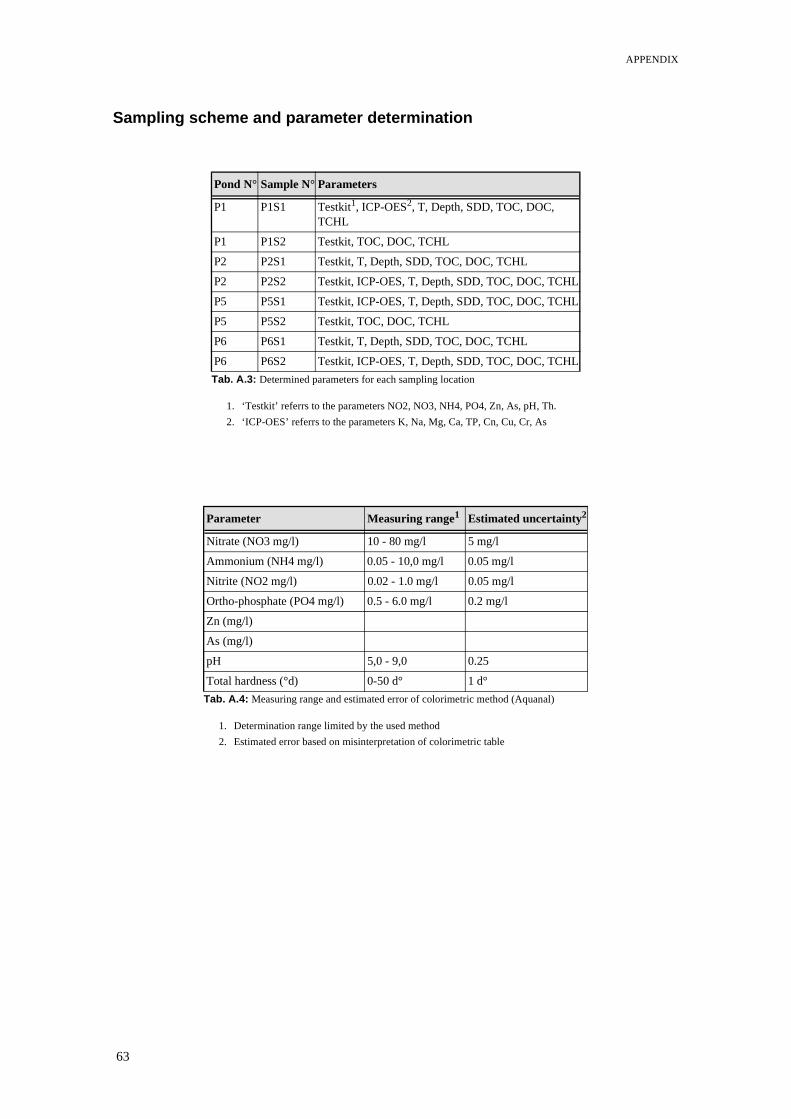
APPENDIX

Sampling scheme and parameter determination

Pond N° Sample N° Parameters

P1 P1S1 Testkit1, ICP-OES2, T, Depth, SDD, TOC, DOC, TCHL

1. ‘Testkit’ referrs to the parameters NO2, NO3, NH4, PO4, Zn, As, pH, Th.

2. ‘ICP-OES’ referrs to the parameters K, Na, Mg, Ca, TP, Cn, Cu, Cr, As

P1 P1S2 Testkit, TOC, DOC, TCHL

P2 P2S1 Testkit, T, Depth, SDD, TOC, DOC, TCHL

P2 P2S2 Testkit, ICP-OES, T, Depth, SDD, TOC, DOC, TCHL


P5 P5S2 Testkit, TOC, DOC, TCHL

P6 P6S1 Testkit, T, Depth, SDD, TOC, DOC, TCHL


Tab. A.3: Determined parameters for each sampling location

Parameter Measuring range1

1. Determination range limited by the used method

Estimated uncertainty2

2. Estimated error based on misinterpretation of colorimetric table

Nitrate (NO3 mg/l) 10 - 80 mg/l 5 mg/l

Ammonium (NH4 mg/l) 0.05 - 10,0 mg/l 0.05 mg/l

Nitrite (NO2 mg/l) 0.02 - 1.0 mg/l 0.05 mg/l

Ortho-phosphate (PO4 mg/l) 0.5 - 6.0 mg/l 0.2 mg/l

Zn (mg/l)

As (mg/l)

pH 5,0 - 9,0 0.25

Total hardness (°d) 0-50 d° 1 d°

Tab. A.4: Measuring range and estimated error of colorimetric method (Aquanal)

63

APPENDIX

Results of limnological measurements

Parameter (unit) P6S2 P6S1 P5S2 P5S1 P2S1 P1S1 P1S2

Depth (m) 0.39 0.50 0.95 n/d 0.70 0.75 n/d

SDD (m) 0.16 0.20 0.95 n/d 0.12 0.10 n/d

Temp Surface (°C) n/d 34.7° 34.8° n/d 35 36.6° n/d

Temp Bottom (°C) n/d 33.6° 34° n/d n/d 35° n/d

Oxygen Saturation (%) n/d n/d n/d n/d n/d n/d n/d

Nitrate (NO3 mg/L) 2 2 5 <5 0 <5 0

Ammonium (NH4 mg/l) <0.05 1 0.2 0.2 0.15 <0.05 <0.05

Calculated ammonia (NH3 mg/L) <0.0025 0.05 0.07 0.07 0.05 <0.0025 <0.0025

Nitrite (NO2 mg/l) <0.02 <0.02 <0.02 0.02 0 <0.02 <0.02

Ortho-Phosphate (PO4 mg/L) 0.1 0.1 0 0 0.1 0 <0.01

ZN (mg/L) bdl bdl 0.1 0.1 0.1 0.4 0.4

AS (mg/L) bdl bdl bdl bdl bdl n/a bdl

pH 9.0 7.6 8.5 8.5 8.5 6.5 6.5

Total hardness (°d) 3 4 6 6 7 <3 <1

TOC (mg/L) 45 42 27 30 33 42 33

DOC (mg/L) 4 3.36 2 2.89 3.19 3.61 2.26

Tab. A.5: Results of limnological parameters determined in India1

1. Results of CHL determination is given in (Tab. 3.3).

Parameter Ganga P1-T3-S1 P2-S1 P5S1b P6S1

K (mg/L) 4 3 26 16 5

Na (mg/L) 8 4 17 26 4

Mg (mg/L) 11 2 10 14 4

Ca (mg/L) 60 4 20 20 12

TP (mg/L) 0.11 0.019 0.032 0.019 0.023

Zn (mg/L) 0.025 0.009 <0.005 <0.005 0.008

Cu (mg/L) 0.017 0.011 0.008 0.005 0.004

Cr (mg/L) <0.001 <0.001 <0.001 <0.001 <0.001

As (mg/L) <0.1 <0.1 0.2 0.2 <0.1

Tab. A.6: Results of ICP-OES determination at EMPA

64

APPENDIX

B. Used methods for parameter extraction

B.I Chlorophyll determination in water samples by Annon`s method

Principle of the method:Spectrophotometric determination of the acetone (80:20, acetone:water) extract of the sample.

Procedure:2 mL of sample was mixed with 8 ml of acetone, kept for ½ hour and then passed through filterpaper Whatman N° 42. The spectrophotometric measures of the extracts were taken at two wave-lengths (645 and 663 nm) and the total chlorophyll content was determined from the followingequation:

, (0.1)

where: Total chlorophyll (mg/g); : Absorbance at 645 nm;: Absorbance at 663 nm;

: Length of light path in a cell (1cm). This is constant and its value is -1;: Final volume of the extract;: Volume (mL) of the water samples.

TC 20.2D645 8.02D663+( ) V×A 1000× W×

-------------------------------------------------------------=

TCD645

D663

AVW

65

APPENDIX

B.II Dissolved organic carbon by dichromate oxidation method of Vance

Principle of the method: In the presence of a strong acid, organic matter is oxidized and Cr (VI) is reduced to Cr (111). Thedichromate left is titrated back.

Procedure:2 mL of 0.1 (N) K2Cr2O7 and 15 mL of acid mixture H2SO4 / H3PO4) were added to 10 mL offiltered (passed through 0.45 µ Millipore membrane filtration assembly) sample in a 250 mLround bottom flask fitted with a Liebig condenser. The whole mixture was gently refluxed for 30minutes, cooled and diluted with 25 mL water, which was added through the condenser as a rinse.The residual dichromate was measured by back titration with 0.01 (N) ferrous ammonium sulfateusing ferroin indicator. At the end point, a sharp color change from green to buff pink took place.

(0.2)

where is the titration solution consumed by the hot (refluxed) blank in mL; is the titration solution consumed by the sample in mL; is the titration solution consumed by the cold (unrefluxed) blank in mL; is the normality of the K2Cr2O7 solution; is the volume of K2Cr207 solution added to the reaction mixture; is the sample taken in mL; =3 (conversion of Cr VI to Cr III)

C H S–( ) M D× E× 1000××C A×

--------------------------------------------------------------------=

HSCMDAE

66

APPENDIX

B.III Total organic carbon by Nelson Somers method

Principle of the methodWet potassium dichromate digestion and titrimetric measurement of unreacted dichromate.

Procedure: 5 mL of 0.4 (N) K2Cr2O7 and 20 mL of H2SO4 were added to 10 mL of filtered sample in a 500mL conical flask. The whole mixture was placed in a hot plate adjusted to 150°C for 30 minutes,cooled and diluted with 200 mL water. The residual dichromate was measured by back titrationwith 0.04 (N) ferrous ammonium sulfate using barium diphenyl sulfate as indicator. At the endpoint, a sharp colour change from blue violet to green took place.

Calculation

(0.3)

whereis the titration solution consumed by the blank in mL; is the titration solution consumed by the sample in mL;is the normality of the ferrous ammonium sulfate solution;

is the sample taken in mL;

Total organic-C (%) = (B - S) x M x 0.003x 100

A

TOC B S–( ) M× 0.003× 100×A

---------------------------------------------------------------=

BSMA

67

APPENDIX

C. Description of additional limnological parameters

Parameter Nitrate

Description There are three important nitrogen compounds which play part in the nitrogencycle: nitrate, nitrite and Ammonia. Depending on the condition (oxygen con-tent) of the media (water), their concentration shifts to either side of the cycle.Nitrogen oxides can get into the environment through natural but also anthro-pogenic ways. Nitrate act as nutrients and have a positive influence on plant growth. There-fore, many fertilizers are based on this substance. The washing out of fertil-ized agricultural grounds leads to high concentrations in the nearby waterbodies. High nitrate concentrations in water bodies support the growth ofplants and algae. The decomposition of the dead biomass produced as a con-sequence of over-fertilization consumes more of dissolved oxygen in thewater than can be reproduced by the plants. As a result of this process(eutrophication), the water body remains in a low-oxygen level with effectson the life forms in the water.A direct toxic effect of nitrate is not known, but a health hazard emerges from

the transformation of nitrate to nitrite in the human body. Other risk to human

health is the supporting of transformation of nitrates to N- nitroso amines.

This compounds have cancerogenetic and mutagenic effect.

Guideline values EU drinking water regulations: max. 50 mg/l Fish water: max. 20 mg/l

Parameter Nitrite

Description Nitrite is a precursor of nitrate from which it is differentiated by

an oxygen atom. During the process of nitrification, proteins are

metabolized to ammonium, then nitrite and finally Nitrate. As

for ammonium, the source of nitrite can be natural (decaying

organic matter) or anthropogenic (faecal, fertilizers). In unpol-

luted water, nitrite concentration is around 0.01 mg/l, which

source is the decomposition of natural nitrogen compounds.

Higher contents are indicators for anthropogenic pollution. High

nitrite concentrations can also be produced by fish excrement.

As for fish nitrite is very toxic, the population has to be reduced.

Nitrite is classified as dangerous to human health. It leads to

obstruction of oxygen transport in the blood, leading to an inter-

nal asphyxiation. Beside, it can produce cancer in the human

body.

Guideline values EU drinking water regulations: max. 0,1 mg/l Fish water: max. 0,03 mg/l

68

APPENDIX

Parameter Ammonium

Description Ammonium (NH4+) is an intermediate which is produced bydecomposition of nitrogenous organic substances. It can get intowater bodies through washing out of fertilized fields. Increasingcontent of ammonium through this way is mostly accompaniedby increasing content of other nitrogenous pollutants. Ammoniacan also be an indicator for discharge of wastewater or sewagedisposal, as it is produced by enzymatic decomposition of urea.Therefore, it is often used as an important indicator of waterquality.

With increasing temperature and pH, ammonium reacts to thetoxic form ammonia, which causes damage to fish.

Guideline values EU drinking water regulations: max. 0,5 mg/lFish water: max. 0,5 mg/l Bathing water (DIN 19643): max. 0,1 mg/l Ammonia: 0.05 for fish water [3]

Parameter Secchi Disk Depth

Description Secchi Disk Depth (SDD) is a limnological measure of water transparency or extinction of light and is widely used to assess trophic state of a water body. It is measured with a black-white disk (secchi disk), which is lowered into the water. SDD is defined as the depth, where the disk can still be seen by human eye.

Guideline values There are no guideline values for SDD.

Parameter Total Hardness

Description The hardness is significantly determined by the calcium saltsdissolved in water. High calcium contents correspond to a highwater hardness which is measured in degrees of German Hard-ness (°d). Water hardness does not cause health problems butaffects the useful properties of the water. In case of fish andaquatic plants, the suitable range of water hardness depends onthe given life forms. Water hardness is determined naturally by the source of thewater: water bodies, which do not originate in springs but in rainwater are usually very soft while water from the subsurface(springs, wells) mostly show high calcium contents. Chemicalpollution can affect the hardness in a significant manner, too.

Guideline values 0 - 4 °d: very soft water4 - 8 °d: soft water8 - 18 °d: medium - hard water18 - 30 °d: hard waterover 30 °d: very hard water

69

APPENDIX

Parameter Organic carbon

Description Organic carbon in freshwater arises from living material(directly from plant photosynthesis or indirectly from terrestrialorganic matter) and also as a constituent of many waste materialsand effluents. Waste discharges high in organic matter and nutri-ents can lead to decreases in DO concentrations as a result of theincreased microbial activity. Consequently, organic matter in thewater can be a useful indication of the degree of pollution.Total organic carbon (TOC) is the sum of organically bound car-bon present in water, bonded to dissolved or suspended matter.

Dissolved organic carbon (DOC) is defined as the sum of organ-ically bound carbon present in water originating from com-pounds which will pass a membrane filter of pore size of 0,45 mm.

Guideline values There are no international guideline values for TOC and DOCfor fish water. Instead, for regular monitoring the following for-mula is often used: The 30-day 50th percentile total organic carbon concentrationshall be within 20% above or below seasonally-adjusted medianbackground levels as measured historically or at appropriatereference sites. In surface waters, TOC concentrations are generally less than 10mg l-1, unless the water receives municipal or industrial wastes,or is highly colored due to natural organic material, as inswamps. In such situations, TOC concentrations may exceed100 mg l-1 TOC concentrations in municipal wastewaters rangefrom 10 to > 100 mg/l, depending on the level of wastewatertreatment. In most surface waters, DOC levels are in the range 1-20 mg/l.[50]

Parameter pH

Description The potential scale of pH values ranges from o to 14. Suchextreme values however do not occur even in heavy pollutedwater. In clean water, pH should be around 7, depending on theenvironment (geology). Animals, especially fish react very sen-sitively to variations of the pH value. Most of them are adaptedto a quite narrow pH range (e.g. trout pH 4 - pH 9)."A shift of the pH value into the basic range (pH value largerthan 7) indicates, among other things, an excessive plant growthin ecological systems (consumption of carbonic acids by theplants) or the presence of pollutants, e. g. suds".

Guideline values There are no guide line values for this parameter.

70

APPENDIX

D. Field sheets

Protocol of ASD field measurements, P..... T.....

Software setup of Instrumentation❑ Adjust computer/WINDOWS time! Is written to ASD measurement header!❑ Adjust FR settings: CONTROL/adjust configurationNumber of samples Spectrum ❑ 10 ❑ 25 ❑ ___

Dark Current (DC) ❑ 10 ❑ 25 ❑ ___White Reference (WR) ❑ 10 ❑ 25 ❑ ___

Fore optics ❑ 25 ❑ 8

Save spectrumpath: C:\Jute\water\date\spectrum base name: <P1>.<T1>.Number of files to save ❑ 001 (single) ❑ ___ (multiple)

Date __. __ .2003

Campaign Jute, 2003

Name of investigator

Location site name:

❑ ASD ❑ GER

Transect-identification: Pond-Nr: P........ Transect-Nr: T........ (or Station-Nr: S........)

GPS coordinates Start: E N, waypoint:

End: E N, waypoint:

Begin / End of experiment(local time)

Start Time : ...... : .......End Time : ...... : .......

Wind conditions ❑ strong ❑ little ❑ none direction: ..........

Photos ❑ yes file name:

WQ measurements: ❑ Yes ❑ No

Stored data under ASD_Laptop: C:\water\yymmdd\spectrum...........................................

backup:....................................................................................

Remarks:

71

APPENDIX

72

Protocol of ASD field measurements P..... T.....

Measurement Waypoint Sky Waves Water color Vegetation Time Groundvisible?

Whiteref.

Remarks:

----------------- Nr. _ _ _ _ _

❑ clear sky❑ diffuse❑ broken clouds

❑ none❑ little❑ big

❑ clear ❑ yellow-brown❑ blue-green ❑ brown❑ yellow ❑ grey

❑ Algae surface % ..... ❑ water plants % .....❑ Algae bottom % ..... ❑ Oil film % .....❑ Reed % ..... ❑ Leaves % .....❑ Bloom Dust % .....

_ _ _ _ _

❑ Yes❑ No

❑ Yes❑ No

----------------- Nr. _ _ _ _ _





_ _ _ _ _

❑ Yes❑ No

❑ Yes❑ No

----------------- Nr. _ _ _ _ _





_ _ _ _ _

❑ Yes❑ No

❑ Yes❑ No

----------------- Nr. _ _ _ _ _





_ _ _ _ _

❑ Yes❑ No

❑ Yes❑ No

----------------- Nr. _ _ _ _ _





_ _ _ _ _

❑ Yes❑ No

❑ Yes❑ No

----------------- Nr. _ _ _ _ _





_ _ _ _ _

❑ Yes❑ No

❑ Yes❑ No

----------------- Nr. _ _ _ _ _





_ _ _ _ _

❑ Yes❑ No

❑ Yes❑ No

----------------- Nr. _ _ _ _ _





_ _ _ _ _

❑ Yes❑ No

❑ Yes❑ No

APPENDIX

APPENDIX

W

WQ

Protocol of Water Quality measurements, No. .........

Date __. __ .2003, ...... : ......

Campaign Jute campaign, 2003

Identification Pond-Nr: ......... Transect-Nr.: ......... (orStation-Nr: .........)According spectral measurement:

GPS coordinates E N waypoint:

Name of investigator

Begin / End of experiment(local time)

Start Time : ...... : .......End Time : ...... : .......

Q-Nr: Parameter Value Units Depth Time Remarks:

.........

73

APPENDIX

Pond Description:

Names of investigator: .................................................................

Date: __. __ .2003, ...... : ......

Campaign: Mai campaign, 2003

Location: Site/village name: .................................................................

Pond Identification: Pond-Nr:

GPS coordinates: E N Waypoint(s): ..............................

saved files: ..............................................................................

Estimated size:...................................

Shoreline vegetation: over water:Reed: ❑ Yes ❑ NoWater Plants: ❑ Yes ❑ NoAlgae: ❑ Yes ❑ No

under water:Algae: ❑ Yes ❑ NoDecayed organic matter: ❑ Yes ❑ No

other: ...........................................................................................................

In-/Outflow ❑ No ❑ Yes: -> Current: ❑ strong ❑ small ❑ absent

Odour of water: ❑ none ❑ fishy ❑ rotten-egg like ❑ ......................... ❑ strong

Retting: ❑ No ❑ Yes: -> ❑ every Year ❑ regularly ❑ few

Last Year: ❑ Yes ❑ No This Year: ❑ No ❑ Yes (Probably)

Retting Type: .....................................................................................

Time of jute in water: ...................................................

Human use: Fishery: ❑ Yes ❑ NoIIrrigation: ❑ Yes ❑ NoSewage disposal: ❑ Yes ❑ No --> Industrial ❑ household ❏

other: ...............................................................................................

Agriculture: Grazing livestock: ❑ Yes ❑ NoFertilizer used: ❑ Yes ❑ No

Ownership: ❑ Private ❑ Public:

74

Determination of water quality parameters in Indian …...Determination of water quality parameters...

Documents

Transcript of Determination of water quality parameters in Indian …...Determination of water quality parameters...