LEGEND - wisconsindot.gov · DRAINAGE FLOW DIRECTION. Title: 11x17 Created Date: 20150518125443Z ...

Wis
con
sin
Hig
hw
ay R
esea
rch
Pro
gra
m
Determination of Typical Resilent Modulus Values
for Selected Soils in Wisconsin SPR# 0092-03-11
Hani H. Titi, Mohammed B. Elias, and Sam Helwany Department of Civil Engineering and Mechanics
UW-Milwaukee
May 2006
WHRP 06-06

Wisconsin Highway Research Program Project ID 0092-03-11
Determination of Typical Resilient Modulus
Values for Selected Soils in Wisconsin
Final Report
Hani H. Titi, Ph.D., P.E.
Associate Professor
Mohammed B. Elias, M.S.
Graduate Research Fellow
and
Sam Helwany, Ph.D., P.E.
Associate Professor
Department of Civil Engineering and Mechanics
University of Wisconsin – Milwaukee
3200 N. Cramer St.
Milwaukee, WI 53211
Submitted to
The Wisconsin Department of Transportation
May 2006

1. Report No. 2. Government Accession No 3. Recipient’s Catalog No
4. Title and Subtitle 5. Report Date
Determination of Typical Resilient Modulus Values for Selected
May 2006
Soils in Wisconsin 6. Performing Organization Code
7. Authors
Hani H. Titi, Mohammed B. Elias, and Sam Helwany
Performing Organization Report No.
8. Performing Organization Name and Address
University of Wisconsin-Milwaukee
Office of Research Services and Administration
Mitchell Hall, Room 273Milwaukee, WI 53201
10. Work Unit No. (TRAIS)
11. Contract or Grant No.
WHRP 0092-03-11
12. Sponsoring Agency Name and Address
Wisconsin Department of Transportation
Division of Transportation Infrastructure Development
Research Coordination Section
4802 Sheboygan Avenue
Madison, WI 53707
13. Type of Report and Period
Covered
14. Sponsoring Agency Code
15. Supplementary Notes
16. Abstract
The objective of this research is to develop correlations for estimating the resilient modulus of various
Wisconsin subgrade soils from basic soil properties. Laboratory testing program was conducted on common
subgrade soils to evaluate their physical and compaction properties. The resilient modulus of the investigated
soils was determined from the repeated load triaxial test following the AASHTO T 307 procedure. The
laboratory testing program produced a high quality and consistent test results database. The high quality test
results were assured through a repeatability study and also by performing two tests on each soil specimen at the
specified physical conditions.
The resilient modulus constitutive equation adopted by NCHRP Project 1-37A was selected for this study.
Comprehensive statistical analysis was performed to develop correlations between basic soil properties and the
resilient modulus model parameters ki. The analysis did not yield good results when the whole test database was
used. However, good results were obtained when fine-grained and coarse-grained soils were analyzed separately.
The correlations developed in this study were able to estimate the resilient modulus of the compacted subgrade
soils with reasonable accuracy. In order to inspect the performance of the models developed in this study,
comparison with the models developed based on LTPP database was made. The LTPP models did not yield good
results compared to the models proposed by this study. This is due to differences in the test procedures, test
equipment, sample preparation, and other conditions involved with development of both LTPP and the models of
this study.
17. Key Words
Resilient modulus, repeated load triaxial test,
Wisconsin soils, statistical analysis,
mechanistic-empirical pavement design.
18. Distribution Statement
No restriction. This document is available to the public
through the National Technical Information Service
5285 Port Royal Road
Springfield, VA 22161
19. Security Classif.(of this report)
Unclassified
19. Security Classif. (of this page)
Unclassified
20. No. of Pages
91
21. Price
ii

Disclaimer
This research was funded through the Wisconsin Highway Research Program by the
Wisconsin Department of Transportation and the Federal Highway Administration under
Project # 0092-03-11. The contents of this report reflect the views of the authors who are
responsible for the facts and the accuracy of the data presented herein. The contents do
not necessarily reflect the official views of the Wisconsin Department of Transportation
or the Federal Highway Administration at the time of publication.
This document is disseminated under the sponsorship of the Department of
Transportation in the interest of information exchange. The United States Government
assumes no liability for its contents or use thereof. This report does not constitute a
standard, specification, or regulation.
The United States Government does not endorse products or manufacturers. Trade and
manufacturers’ names appear in this report only because they are considered essential to
the object of the document.
iii

Abstract
The objective of this research is to develop correlations for estimating the resilient
modulus of various Wisconsin subgrade soils from basic soil properties. Laboratory
testing program was conducted on common subgrade soils to evaluate their physical and
compaction properties. The resilient modulus of the investigated soils was determined
from the repeated load triaxial test following the AASHTO T 307 procedure. The
laboratory testing program produced a high quality and consistent test results database.
The high quality test results were assured through a repeatability study and also by
performing two tests on each soil specimen at the specified physical conditions.
The resilient modulus constitutive equation adopted by NCHRP Project 1-37A was
selected for this study. Comprehensive statistical analysis was performed to develop
correlations between basic soil properties and the resilient modulus model parameters ki.
The analysis did not yield good results when the whole test database was used. However,
good results were obtained when fine-grained and coarse-grained soils were analyzed
separately. The correlations developed in this study were able to estimate the resilient
modulus of the compacted subgrade soils with reasonable accuracy. In order to inspect
the performance of the models developed in this study, comparison with the models
developed based on LTPP database was made. The LTPP models did not yield good
results compared to the models proposed by this study. This is due to differences in the
test procedures, test equipment, sample preparation, and other conditions involved with
development of both LTPP and the models of this study.
iv

Acknowledgement
This research project is financially supported by the Wisconsin Department of
Transportation (WisDOT) through the Wisconsin Highway Research Program (WHRP).
The authors would like to acknowledge the WisDOT Project Research Committee: Bruce
Pfister, Steven Krebs, and Tom Brokaw, for their guidance and valuable input in this
research project. The authors also would like to thank Robert Arndorfer, WHRP
Geotechnical TOC Chair for his support and Dennis Althaus for his effort and help in
collecting soil samples.
The research team would like to thank many people at UW-Milwaukee who helped in the
accomplishment of the research project, namely: Joe Holbus who manufactured the
special compaction molds, Jaskaran Singh who helped in performing experimental testing
on different soils, Dan Mielke, who helped in soil properties testing, and Rahim Reshadi,
who helped in various stages during the assembly of the dynamic materials test system.
The effort and help of Adam Titi during the preparation of the report is appreciated. The
authors would like to thank Dr. Marjorie Piechowski for the valuable comments on the
final report.
v

Table of Contents
Abstract…………………………………………………………………………………...... iv
Acknowledgement………………………………………………………………………... v
List of Tables……………………………………………………………………………….. viii
List of Figures………………………………………………………………………............ x
Executive Summary ………………………………………………………………………. xii
Chapter 1: Introduction…………………………………………………………............... 1
1.1 Problem Statement………………………………………………………….. 1
1.2 Research Objectives……………………………………………………….... 2
1.3 Scope……………………………………………………………………….. 2
1.4 Research Report……………………………………………………………. 3
Chapter 2: Background…………………………………………………………………... 4
2.1 Determination of Resilient Modulus of Soils….………………………........ 4
2.2 Factors Affecting Resilient Modulus of Subgrade Soils……………………. 8
2.2.1 Soil Physical Conditions….…….………………………………….... 8
2.2.2 Effect of Loading Conditions ……………………………………….. 8
2.2.3 Other Factors Affecting Resilient Modulus of Subgrade Soils……… 9
2.3 Resilient Modulus Models ………………………………… ………………. 10
2.4 Mechanistic – Empirical Pavement Design ……………………………….. . 13
2.5 Soil Distributions in Wisconsin .……………………………………………. 14
Chapter 3: Research Methodology ………………………………………………………. 18
vi

3.1 Investigated Soils………………………………………………………….. 18
3.2 Laboratory Testing Program………………………………………………. 18
3.2.1 Physical Properties and Compaction Characteristics ……………… 18
3.2.2 Repeated Load Triaxial Test ………………………………………. 21
Chapter 4: Test Results and Analysis…………………………………………………… 28
4.1 Properties of the Investigated Soils ………………………………………. 28
4.2 Resilient Modulus of the Investigated Soils………………………………. 34
4.3 Statistical Analysis ……………………………………………………….. 51
4.3.1 Evaluation of the Resilient Modulus Model Parameters …………... 51
4.3.2 Correlations of Model Parameters with Soil Properties……………. 53
4.3.3 Statistical Analysis Results ………………………………………… 57
4.4 Predictions Using LTPP Models…………………………………………... 81
Appendix A
Appendix B
Chapter 5: Conclusions and Recommendations………………………………………... 86
References ………………………………………………………………………………… 88
vii

List of Tables
Table 2.1: Wisconsin pedological soil groups (After Hole 1980)…………........................ 14
Table 3.1: Standard tests used in this investigation………………………………………... 21
Table 4.1: Properties of the investigated soils …………………………………………….. 29
Table 4.2: Results of the standard compaction test on the investigated soils ……………... 37
Table 4.3: Typical results of the repeated load triaxial test conducted according to
AASHTO T 307 ...…………………………………………………...................... 38
Table 4.4: Analysis of repeatability tests on Dodgeville soil tested at maximum dry unit
weight and optimum moisture content …………...………………………………
Table 4.5: Analysis of repeatability tests on Dodgeville soil tested at 95% of maximum
dry unit weight and moisture content less than the optimum moisture content
(dry side)………………………………………….. …………………..................
Table 4.6: Analysis of repeatability tests on Dodgeville soil tested at 95% of maximum
dry unit weight and moisture content greater than the optimum moisture content
(wet side)…………………………………………………………... ………….....
Table 4.7: Basic statistical data of the resilient modulus model parameters ki obtained
from the test results of the investigated soils…………………..…………………
46
47
48
53
Table 4.8: Constituents of the investigated soils……………............................................... 58
Table 4.9: Correlations between the resilient modulus model parameter k1 and basic soil
properties for fine grained-soils………………………………………………......
Table 4.10: Correlations between the resilient modulus model parameter k2 and basic soil
properties for fine grained-soils…………………………...……………………...
Table 4.11: Correlations between the resilient modulus model parameter k3 and basic soil
properties for fine grained-soils………………………….. ……………………...
Table 4.12: Correlation matrix of model parameters and soil properties for fine-grained
soils…………………………………………………………... ……………….....
59
59
60
64
Table 4.13: Summary of t-statistics for regression coefficients used in resilient modulus
model parameters for fine-grained soils……….……………... ……………….....
Table 4.14: Characteristics of particle size distribution curves of investigated coarse-
grained soils…………………………………………………................................
Table 4.15 Correlations between the resilient modulus model parameter k1 and basic soil
properties for non-plastic coarse grained soils.……………....…………………...
Table 4.16: Correlations between the resilient modulus model parameter k2 and basic soil
properties for non-plastic coarse grained soils……………... ………...………….
Table 4.17: Correlations between the resilient modulus model parameter k3 and basic soil
properties for non-plastic coarse grained soils……………....................................
Table 4.18: Correlation matrix of model parameters and soil properties for non-plastic
coarse-grained soils……………... ………………………….................................
64
66
67
67
68
72
viii

Table 4.19: Summary of t-statistics for regression coefficients used in resilient modulus
model parameters for non-plastic coarse-grained soils……………………...….. 72
Table 4.20: Correlations between the resilient modulus model parameter k1 and basic soil
properties for plastic coarse-grained soils….……………...................................... 74
Table 4.21: Correlations between the resilient modulus model parameter k2 and basic soil
properties for plastic coarse-grained soils………………………………………... 74
Table 4.22: Correlations between the resilient modulus model parameter k3 and basic soil
properties for plastic coarse-grained soils……………... ………………………... 75
Table 4.23: Correlation matrix of model parameters and soil properties for plastic coarse-
grained soils …………………………………...……………................................ 79
Table 4.24: Summary of t-statistics for regression coefficients used in resilient modulus
model parameters for plastic coarse-grained soils ……………...……………..… 79
ix

List of Figures
Figure 2.1: Repeated load triaxial test setup ( Instron 8802 dynamic materials test
system)…………………………………………………………………………… 5
Figure 2.2: Definition of the resilient modulus in a repeated load triaxial test …………… 6
Figure 2.3: Schematic of soil specimen in a triaxial chamber according to AASHTO T
307 ………………………………………………………………………………………… 7
Figure 2.4: Wisconsin pedological soil groups (Hole, 1980) …………………………….. 15
Figure 2.5: Wisconsin Soil Regions, Madison and Gundlach (1993) …………………….. 17
Figure 3.1: Locations of the investigated Wisconsin soils………………………………… 19
Figure 3.2: Pictures of some of the investigated Wisconsin soils ....……………………… 20
Figure 3.3: The UWM servo-hydraulic closed-loop dynamic material test system used in
this study ………………………………………………………………………… 22
Figure 3.4: Special mold designed to compact soil specimens according to AASHTO T
307 requirements ……………………………………………………………….. 24
Figure 3.5: Conditions of unit weight and moisture content under which soil specimens
were subjected to repeated load triaxial test……………………...…………….. 25
Figure 3.6: Preparation of soil specimen for repeated load triaxial test……...…………... 26
Figure 3.7: Computer program used to control and run the repeated load triaxial test for
determination of resilient modulus……………………………....……………… 27
Figure 4.1: Particle size distribution curve of Dodgeville soil……....……………………. 32
Figure 4.2: Results of Standard Proctor test for Dodgeville soil ....……………...………. 32
Figure 4.3: Particle size distribution curve of Antigo soil…….. ....………………………. 33
Figure 4.4: Results of Standard Proctor test for Antigo soil…... ....…………..…………... 33
Figure 4.5: Particle size distribution curve of Plano soil....……………………….………. 35
Figure 4.6: Results of Standard Proctor test for Plano soil ….....………………….……… 35
Figure 4.7: Particle size distribution curve of Kewaunee soil-1…………………......……. 36
Figure 4.8: Results of Standard Proctor test for Kewaunee soil-1………………..……….. 36
x

Figure 4.9: Results of repeated load triaxial test on Antigo soil compacted at 95% of
maximum dry unit weight (Jdmax) and moisture content more than wopt. (wet
side)……………………………………………………………………………... 39
Figure 4.10: Results of repeated load triaxial test on Dodgeville soil compacted at
maximum dry unit weight (Jdmax) and optimum moisture content (wopt.)…….. ... 41
Figure 4.11: Results of repeated load triaxial test on Dodgeville soil compacted at 95%
of maximum dry unit weight (Jdmax) and moisture content less than wopt. (dry
side)……............................................................................................................... 43
Figure 4.12: Results of repeated load triaxial test on Dodgeville soil compacted at 95%
of maximum dry unit weight (Jdmax) and moisture content more than wopt. (wet
side)....................................................................................................................... 45
Figure 4.13: The effect of unit weight and moisture content on the resilient modulus of
the investigated soils……………………………………………………………. 49
Figure 4.14: The effect of the moisture content on the resilient modulus of the
investigated soils ……………………………………………………………….. 50
Figure 4.15: Histograms of resilient modulus model parameters ki obtained from
statistical analysis on the results of the investigated Wisconsin soils................... 45
Figure 4.16: Comparison of resilient modulus model parameters (ki) estimated from soil
properties and ki determined from results of repeated load triaxial test on
investigated fine-grained soils ………………………………………………….. 61
Figure 4.17: Predicted versus measured resilient modulus of compacted fine-grained
soils……………………………………………………………………………... 65
Figure 4.18: Comparison of resilient modulus model parameters (ki) estimated from soil
properties and ki determined from results of repeated load triaxial test on
investigated non-plastic coarse-grained soils….................................................... 69
Figure 4.19: Predicted versus measured resilient modulus of compacted non-plastic
coarse-grained soils …………………………………………………………….. 73
Figure 4.20: Comparison of resilient modulus model parameters (ki) estimated from soil
properties and ki determined from results of repeated load triaxial test on
investigated plastic coarse-grained soils ……………………………………….. 76
Figure 4.21: Predicted versus measured resilient modulus of compacted plastic coarse-
grained soils.......................................................................................................... 80
Figure 4.22: Predicted versus measured resilient modulus of Wisconsin fine-grained
soils using the mode developed in this study and the LTPP database developed
models….………………………………………………………………………… 83
Figure 4.23: Predicted versus measured resilient modulus of Wisconsin non-plastic
coarse-grained soils using the mode developed in this study and the LTPP
database developed models……………………………………………………..... 84
Figure 4.24: : Predicted versus measured resilient modulus of Wisconsin plastic coarse-
grained soils using the mode developed in this study and the LTPP database
developed models ………………………………………………………………... 85
xi

Executive Summary
A major effort was undertaken by the National Cooperative Highway Research Program
(NCHRP) to develop Mechanistic-Empirical pavement design procedures based on the
existing technology in which state of the art models and databases are utilized. The
NCHRP project 1-37A: “Development of the 2002 Guide for Design of New and
Rehabilitated Pavement Structures” was completed and the final report and software was
published on July 2004. The outcome of the NCHRP project 1-37A is the “Guide for
Mechanistic-Empirical Design of New and Rehabilitated Pavement Structures,” which is
currently undergoing extensive evaluation and review by state highway agencies across
the country.
Currently, the Wisconsin Department of Transportation uses the AASHTO 1972 Design
Guide for flexible pavement design in which the SSV is used to characterize subgrade
soils. There is a need to adopt the mechanistic-empirical methodology for pavement
design and rehabilitation in Wisconsin, which uses the resilient modulus to characterize
subgrade soils. The mechanistic-empirical approach takes into account several important
variables such as repeated loading, environmental conditions, pavement materials, and
subgrade materials. The mechanistic-empirical pavement design should significantly
reduce variations in pavement performance as related to design life and produce
significant savings from reductions in premature failures and lower maintenance over the
life cycle of the pavements.
The Wisconsin Department of Transportation is currently reviewing and evaluating the
new guide for adoption and implementation in the design of pavement structures. The
new mechanistic-empirical pavement design guide requires design input parameters that
were not previously evaluated by WisDOT for pavement design such as the resilient
modulus of Wisconsin subgrade soils. However, conducting resilient modulus tests
requires specialized and expensive equipment. In addition, the resilient modulus test is
laborious and time consuming. These limitations signify the need for developing
methodologies to reliably estimate the resilient modulus of Wisconsin subgrade soils
based on correlations with fundamental soil properties.
This research project was initiated to develop correlations for estimating the resilient
modulus of various Wisconsin subgrade soils from basic soil properties. A laboratory
testing program was conducted on common subgrade soils to evaluate their physical and
compaction properties. The resilient modulus of the investigated soils was determined
from the repeated load triaxial test following the AASHTO T 307 procedure. The
laboratory testing program produced a high quality and consistent test results database.
The high quality test results were assured through a repeatability study and also by
performing two tests on each soil specimen at the specified physical conditions.
The resilient modulus constitutive equation adopted by NCHRP Project 1-37A was
selected for this study. Comprehensive statistical analysis was performed to develop
correlations between basic soil properties and the resilient modulus model parameters ki.
xii

The analysis did not yield good results when the whole test database was used. However,
good results were obtained when fine-grained and coarse-grained soils were analyzed
separately. The correlations developed in this study were able to estimate the resilient
modulus of the compacted subgrade soils with reasonable accuracy. In order to inspect
the performance of the models developed in this study, comparison with the models
developed based on LTPP database was made. The LTPP models did not yield good
results compared to the models proposed by this study. This is due to differences in the
test procedures, test equipment, sample preparation, and other conditions involved with
development of both LTPP and the models of this study.
The results of the repeated load triaxial test on the investigated Wisconsin subgrade soils
provide resilient modulus database that can be utilized to estimate values for mechanistic-
empirical pavement design in the absence of basic soils testing (level 3 input parameters).
The equations, developed herein, that correlate resilient modulus model parameters (k1,
k2, and k3) to basic soil properties for fine-grained and coarse-grained soils can be utilized
to estimate level 2 resilient modulus input for the mechanistic-empirical pavement
design. These equations (correlations) are based on statistical analysis of laboratory test
results that were limited to the soil physical conditions specified. Estimation of resilient
modulus of subgrade soils beyond these conditions was not validated.
xiii

Chapter 1
Introduction
1.1 Problem Statement
The design and evaluation of pavement structures on base and subgrade soils requires a
significant amount of supporting data such as traffic loading characteristics, base,
subbase and subgrade material properties, environmental conditions and construction
procedures. Currently, empirical correlations developed between field and laboratory
material properties are used to obtain highway performance characteristics (Barksdale et
al., 1990). These correlations do not satisfy the design and analysis requirements since
they neglect all possible failure mechanisms in the field. Also, most of these methods,
which use California Bearing Ratio (CBR) and Soil Support Value (SSV), do not
represent the conditions of a pavement subjected to repeated traffic loading. Recognizing
this deficiency, the 1986 and the subsequent 1993 American Association of State
Highway and Transportation Officials (AASHTO) design guides recommended the use of
resilient modulus (Mr) for characterizing base and subgrade soils and for designing
flexible pavements. The resilient modulus accounts for soil deformation under repeated
traffic loading with consideration of seasonal variations of moisture conditions.
A major effort was recently undertaken by the National Cooperative Highway Research
Program (NCHRP) to develop Mechanistic-Empirical pavement design procedures based
on the existing technology in which state of the art models and databases are utilized. The
NCHRP project 1-37A: “Development of the 2002 Guide for Design of New and
Rehabilitated Pavement Structures” was recently completed and the final report and
software was published on July 2004. The outcome of the NCHRP project 1-37A is the
“Guide for Mechanistic-Empirical Design of New and Rehabilitated Pavement
Structures,” which is currently undergoing extensive evaluation and review by state
highway agencies across the country.
Currently, the Wisconsin Department of Transportation (WisDOT) uses the AASHTO
1972 Design Guide for flexible pavement design in which the SSV is used to characterize
subgrade soils. There is a need to adopt the mechanistic-empirical methodology for
pavement design and rehabilitation in Wisconsin, which uses the resilient modulus to
characterize subgrade soils. The mechanistic-empirical approach takes into account
several important variables such as repeated loading, environmental conditions, pavement
materials, and subgrade materials. The mechanistic-empirical pavement design should
significantly reduce variations in pavement performance as related to design life and
produce significant savings from reductions in premature failures and lower maintenance
over the life cycle of the pavements (NCHRP Project 1-37A Summary, 2000 and 2001).
Therefore, WisDOT is currently reviewing and evaluating the new guide for adoption and
implementation in the design of pavement structures. The new mechanistic-empirical
pavement design guide requires design input parameters that were not previously
1

evaluated by WisDOT for pavement design such as the resilient modulus of Wisconsin
subgrade soils. However, conducting resilient modulus tests requires specialized and
expensive equipment. In addition, the resilient modulus test is laborious and time
consuming. These limitations signify the need for developing methodologies to reliably
estimate the resilient modulus of Wisconsin subgrade soils based on correlations with
fundamental soil properties.
1.2 Research Objectives
The primary objective of this research project is to develop a methodology for estimating
the resilient modulus of various Wisconsin subgrade soils from basic soil properties. The
following specific objectives are identified for successful accomplishment of this
research:
1. To conduct repeated load triaxial tests to determine resilient modulus of
representative Wisconsin subgrade soils. WisDOT engineers and the research
team will select these “typical” subgrade soils. The focus is on investigating the
effect of soil type, soil physical properties, stress level, and environmental
conditions on the resilient modulus of the selected soils. This work establishes a
test result database that is used to develop correlations between various soil
properties and the resilient modulus model parameters.
2. To develop and validate correlations (models) between soil properties and the
resilient modulus model parameters. Applicability of theoretical and statistical
methods for developing these correlations is investigated.
1.3 Scope
The laboratory-testing program is conducted on selected soils that are considered
representative of the soil distributions in Wisconsin. The repeated load triaxial test is
conducted to determine the resilient modulus of the selected soils according to the
standard procedure: AASHTO T 307. Other laboratory tests are conducted following
standard test procedures that are used by WisDOT. The resilient modulus correlations
with soil properties, that are developed and validated, are based on the results of the
experimental testing program.
1.4 Research Report
This report summarizes the research effort conducted at the University of Wisconsin-
Milwaukee (UWM) to evaluate resilient modulus of common Wisconsin subgrade soils.
A laboratory testing program was conducted on soils representative of the soil
distributions of Wisconsin. Laboratory testing was conducted to evaluate basic properties
and to determine the resilient modulus of the investigated soils. Comprehensive statistical
analysis was performed to develop correlations between basic soil properties and the
resilient modulus model input parameters. The resilient modulus model is the constitutive
equation developed by NCHRP project 1-28A and adopted by the NCHRP project 1-37A
2
for the “Guide for Mechanistic-Empirical Design of New and Rehabilitated Pavement
Structures.”
This report is organized in five chapters. Chapter One presents the problem statement,
objectives and scope of the study. Background information on resilient modulus of
subgrade soils is summarized in Chapter Two. Chapter Three describes the research
methodology and laboratory-testing program conducted on Wisconsin subgrade soils.
Chapter Four presents the test results, statistical analysis, and the models developed to
estimate the resilient modulus of Wisconsin subgrade soils from basic soil properties.
Finally, Chapter Five presents the conclusions and recommendations of the study.
3

Chapter 2
Background
This chapter presents background information on the resilient modulus of subgrade soils.
The information includes a description of the repeated load triaxial test, factors affecting
resilient modulus, and models used to estimate the resilient modulus for pavement design
and rehabilitation. In addition, background information on Wisconsin soils is also
presented.
2.1 Determination of Resilient Modulus of Soils
Several laboratory and field nondestructive test methods have been used to determine
resilient modulus of subgrade soils. Laboratory test methods include the repeated load
triaxial test, which is the most commonly used method for the determination of resilient
modulus of soils. Field nondestructive test methods using Dynaflect and Falling Weight
Deflectometer (FWD) have been used to estimate the resilient modulus of subgrade soils
under existing pavements. Deflection measurements of pavement layers are used through
backcalculation subroutines to estimate the resilient properties. Both laboratory and field
methods are improving with new developments in hardware technologies, particularly in
data acquisition systems and computer technology.
The repeated load triaxial test is specified for determining the resilient modulus by
AASHTO T 294: “Resilient Modulus of Unbound Granular Base/Subbase Materials and
Subgrade Soils-SHRP Protocol P 46,” and by AASHTO T 307: “Determining the Resilient Modulus of Soils and Aggregate Materials.” The repeated load triaxial test
consists of applying a cyclic load on a cylindrical specimen under constant confining
pressure (V3 or Vc ) and measuring the axial recoverable strain (Hr). The repeated load
triaxial test setup is shown in Figure 2.1.
The system consists of a loading frame with a crosshead mounted hydraulic actuator. A
load cell is attached to the actuator to measure the applied load. The soil sample is housed
in a triaxial cell where confining pressure is applied. As the actuator applies the repeated
load, sample deformation is measured by a set of Linear Variable Differential
Transducers (LVDT’s). A data acquisitions system records all data during testing.
The resilient modulus determined from the repeated load triaxial test is defined as the
ratio of the repeated axial deviator stress to the recoverable or resilient axial strain:
V dM r (2.1)H r
where Mr is the resilient modulus, Vd is the deviator stress (cyclic stress in excess of
confining pressure), and Hr is the resilient (recoverable) strain in the vertical direction.
4
Figure 2.2 depicts a graphical representation of the definition of resilient modulus from a
repeated load triaxial test.
AASHTO provided standard test procedures for determination of resilient modulus using
the repeated load triaxial test, which include AASHTO T 292, AASHTO T 294 and
AASHTO T 307. There were some problems and issues associated with some
procedures, which were improved with time. The AASHTO T 307 is the current protocol
for determination of resilient modulus of soils and aggregate materials. It evolved from
the Long Term Pavement Performance (LTPP) protocol P46. Detailed background and
discussion on AASHTO T 307 is presented by Groeger et al. (2003).
Figure 2.1: Repeated load triaxial test setup (Instron 8802 dynamic materials test
system)
5

Str
ess
(V��o
r S
trai
n (H�
Dev
iato
r L
oad
(k
N)
0.1 0.9
Time (s)
(a) Shape and duration of repeated load
Resilient strain, H r
Strain
Dev
iato
r st
ress
, V
d
Plastic strain, H p
Time (t)
Stress
(b) Stresses and strains of one load cycle
Figure 2.2: Definition of the resilient modulus in a repeated load triaxial test
6

AASHTO T 307 requires a haversine-shaped loading waveform as shown in Figure 2.2a.
The load cycle duration, when using a hydraulic loading device, is 1 second that includes
a 0.1 second load duration and a 0.9 second rest period. The repeated axial load is applied
on top of a cylindrical specimen under confining pressure. The total recoverable axial
deformation response of the specimen is measured and used to calculate the resilient
modulus. AASHTO T 307 requires the use of a load cell and deformation devices
mounted outside the triaxial chamber. Air is specified as the confining fluid, and the
specimen size is required to have a minimum diameter to length ratio of 1:2. Figure 2.3
shows a schematic of soil specimen in a triaxial chamber according to AASHTO T 307
requirements.
Figure 2.3: Schematic of soil specimen in a triaxial chamber according to AASHTO
T 307
7

2.2 Factors Affecting Resilient Modulus of Subgrade Soils
Factors that influence the resilient modulus of subgrade soils include physical condition
of the soil (moisture content and unit weight), stress level and soil type. Many studies
have been conducted to investigate these effects on the resilient modulus. For example,
Zaman (1994) reported that the results of the repeated load triaxial test depend on soil
gradation, compaction method, specimen size and testing procedure. The effect of some
of these factors on the resilient modulus of subgrade soils is significant. Li and Selig
(1994) reported that a resilient modulus range between 14 and 140 MPa can be obtained
for the same fine-grained subgrade soil by changing parameters such as stress state or
moisture content. Therefore, it is essential to understand the factors affecting the resilient
modulus of subgrade soils.
2.2.1 Soil Physical Conditions
Research studies showed that the moisture content and unit weight (or density) have a
significant effect on the resilient modulus of subgrade soils. The resilient modulus of
subgrade soil decreases with the increase of the moisture content or the degree of
saturation (Barksdale 1972, Fredlund 1977, Drumm et al. 1997, Huang 2001, Butalia
2003, and Heydinger 2003). Butalia et al. (2003) investigated the effects of moisture
content and pore pressures buildup on the resilient modulus of Ohio soils. Tests on
unsaturated cohesive soils showed that the resilient modulus decreases with the increase
in moisture content.
Drumm et al. (1997) studied the variation of resilient modulus with a post-compaction
increase in moisture content. Soil samples were compacted at maximum dry unit weight
and optimum moisture content; then the moisture content was increased. Investigated
soils exhibited a decrease in resilient modulus with the increase in saturation. Heydinger
(2003) stated that moisture content is the primary variable for predicting seasonal
variation of resilient modulus of subgrade soils.
The effect of unit weight on the resilient modulus of subgrade soils also has been largely
investigated (e.g., Smith and Nair 1973, Chou 1976, Allen 1996, Drumm 1997). Test
results indicated that the resilient modulus increases with the increase of the dry unit
weight (density) of the soil. However, this effect is small compared to the effect of
moisture content and stress level on resilient modulus (Rada and Witczak 1981). At any
dry unit weight (density) level, the resilient modulus has two values: one when the soil is
tested under dry of optimum moisture content and another value when the soil is tested
under wet of optimum moisture content. The resilient modulus of the soil compacted on
the dry side of optimum is larger than that when the soil is compacted at the wet of
optimum.
2.2.2 Effect of Loading Conditions
The resilient modulus is a stress-dependent soil property as it is a measure of soil
stiffness. According to Rada and Witczak (1981), the most significant loading condition
8

factor that affects resilient modulus response is the stress level. In general, the increase in
the deviator stress results in decreasing the resilient modulus of cohesive soils due to the
softening effect. The increase of the confinement results in an increase in the resilient
modulus of granular soils. Lekarp et al. (2000) reported that the confining pressure has
more effect on material stiffness than deviator or shear stress.
Rada and Witczak (1981) reported that for loading characteristics, factors such as stress
duration, stress frequency, sequence of load and number of stress repetitions necessary to
reach an equilibrium-resilient strain response have little effect on resilient modulus
response.
Laboratory investigations of the effect of stress history on the resilient modulus results
showed that the resilient modulus increases with the increase of the repeated number of
loads. This increase was mainly attributed to the reduction in moisture content of the soil.
AASHTO T 307 requires the specimen to undergo 500-1000 conditioning cycles before
testing to provide a uniform contact between the soil specimen and the top and bottom
platens. However, Pezo et al. (1992) and Nazarian and Feliberti (1993) reported that
specimen conditioning affected the resilient modulus of the specimen and indicated that
stress history plays an important role in the modulus of soils.
Effect of Confining Stress
Most laboratory studies on subgrade soils and unbound materials show that the resilient
modulus increases with the increase of the confining stress (Seed et al. 1962, Thomson
and Robnett 1976, Rada and Witczak 1981, and Pezo and Hudson 1994). Thompson and
Robnett (1979) concluded that the resilient modulus of fine-grained soils does not depend
on the confining pressure and that confining pressures in the upper soil layers under
pavements are normally less than 35 kPa (5 psi). In general, the effect of confining stress
is more significant in granular soils than in fine-grained soils. For granular materials, the
increase in confining pressure can significantly increase the resilient modulus (Rada and
Witczak 1981). Resilient modulus of coarse-grained materials is usually described as a
function of bulk stress.
Effect of Deviator Stress
The resilient modulus of cohesive soils is significantly influenced by the deviator stress.
The resilient modulus of fine-grained soils decreases with the increase of the deviator
stress. For granular materials, the resilient modulus increases with increasing deviator
stress, which typically indicates strain hardening due to reorientation of the grains into a
denser state (Maher et al. 2000). Resilient modulus of cohesive soils is usually described
as a function of deviator stress.
2.2.3 Other Factors Affecting Resilient Modulus of Subgrade Soils
There are other factors that affect the resilient modulus of subgrade soils. These factors
include soil type and properties such as amount of fines and plasticity characteristics. In
9

addition, the sample preparation method and the sample size have influence on the test
results. Material stiffness is affected by particle size and particle size distribution.
Thompson and Robnett (1979) reported that low clay content and high silt content results
in lower resilient modulus values. Thompson and Robnett (1979) also showed that low
plasticity index and liquid limit, low specific gravity, and high organic content result in
lower resilient modulus. Other research results indicated that the amount of fines has no
general trend on the resilient modulus of granular materials (Chou 1976). Lekarp et al.
(2000) reported that the resilient modulus generally decreases when the amount of fines
increases. Janoo and Bayer II (2001) noticed an increase in the resilient modulus with the
increase in maximum particle size.
Seed et al. (1962) reported that the compaction method used to prepare soil samples
affected the resilient modulus response. In general, samples that were compacted
statically showed higher resilient modulus compared to those prepared by kneading
compaction.
Cycles of freezing and thawing may have a significant influence on the resilient modulus
of the pavement system. Scrivner et al. (1989) reported that freezing results in a sharp
reduction in surface deflections while thawing produces an immediate deflection
increase. Chamberlain (1969) reported that the decrease in resilient modulus
accompanying freezing and thawing was caused by the increase in moisture content and
decrease in unit weight.
In addition to the above mentioned factors, other factors of minor effects on the resilient
modulus of subgrade soils were also investigated. Pezo and Hudson (1994) correlated the
resilient modulus to the soil specimen age and plasticity index. They showed that the
older the specimen is at the time of testing, the less the resilient strain, which indicates
higher resilient modulus.
2.3 Resilient Modulus Models
Mathematical models are generally used to express the resilient modulus of subgrade
soils such as the bulk stress model and the deviatoric stress model. These models were
utilized to correlate resilient modulus with stresses and fundamental soil properties. A
valid resilient modulus model should represent and address most factors that affect the
resilient modulus of subgrade soils.
Bulk Stress Model
The bulk stress (T or Vb) is the sum of the principal stresses V1, V2, and V3. The bulk
stress is considered a major factor for estimating the resilient modulus of granular soils.
The resilient modulus can be estimated using the bulk stress from the following equation:
2M r k1T k (2.2)
10
where Mr is the resilient modulus, T is the bulk stress =V1 �V 2 �V 3 , and k1 and k2 are
material constants.
Although this model was used to characterize the resilient modulus of granular soils, it
does not account for shear stress/strain and volumetric strain. Uzan (1985) demonstrated
that the bulk stress model does not sufficiently describe the behavior of granular
materials.
May and Witczak (1981) modified the bulk stress model by adding a new factor as
follows:
2M K k T k (2.3)r 1 1
where K1 is a function of pavement structure, test load and developed shear strain.
Deviatoric Stress “Semi- log” Model
The deviator stress is the cyclic stress in excess of confining pressure. The resilient
modulus of cohesive soils is a function of the deviatoric stress, as it decreases with
increasing the deviatoric stress. The deviatoric stress model was recommended by
AASHTO to estimate resilient modulus of cohesive soils. In the deviatoric stress model,
the resilient modulus is expressed by the following equation:
4M r k3V dk
(2.4)
where Vd is the deviator stress and k3 and k4 are material constants.
The disadvantage of the deviatoric stress model is that it does not account for the effect of
confining pressure. Li and Selig (1994) reported that for fine-grained soils the effect of
confining pressure is much less significant than the effect of deviatoric stress. However,
cohesive soils that are subjected to traffic loading are affected by confining stresses.
Uzan Model
Uzan (1985) studied and discussed different existing models for estimating resilient
modulus. He developed a model to overcome the bulk stress model limitations by
including the deviatoric stress to account for the actual field stress state. The model
defined the resilient modulus as follows:
2 3M k T k V k (2.5)r 1 d
where k1, k2, and k3 are material constants and T and Vd are the bulk and deviatoric
stresses, respectively.
11

By normalizing the resilient modulus and stresses in the above model, it can be written as
follows:
ª T ºk2 ªV d
ºk3
M r k1 Pa (2.6)« » « »P P¬ a ¼ ¬ a ¼
where Pa is the atmospheric pressure, expressed in the same unit as Mr, Vd and T.
Uzan also suggested that the above model can be used for all types of soils. By setting k3
to zero the bulk model is obtained, and the semi-log model can be obtained by setting k2
to zero.
Octahedral Shear Stress Model
The Uzan model was modified by Witzak and Uzan (1988) by replacing the deviatoric
stress with octahedral shear stress as follows:
ª ºk2 ªW º
k3T octM k P (2.7)r 1 a « » « »P P¬ a ¼ ¬ a ¼
where Woct is the octahedral shear stress, Pa is the atmospheric pressure, and k1, k2, and k3
are material constants.
AASHTO Mechanistic-Empirical Pavement Design Models
The general constitutive equation (resilient modulus model) that was developed through
NCHRP project 1-28A was selected for implementation in the upcoming mechanistic-
empirical AASHTO Guide for the Design of New and Rehabilitated Pavement Structures.
The resilient modulus model can be used for all types of subgrade materials. The resilient
modulus model is defined by (NCHRP 1-28A):
§V · k2 §W ·
k3
b octM r k1Pa ̈¸ ¨ �1¸ (2.8)¨ ¸ ¨ ¸P P© a ¹ © a ¹
where:
Mr = resilient modulus
Pa = atmospheric pressure (101.325 kPa)
Vb = bulk stress = V1 + V2+ V3
V1 = major principal stress
V2 = intermediate principal stress = V3 for axisymmetric condition (triaxial test)
V3 = minor principal stress or confining pressure in the repeated load triaxial test
Woct = octahedral shear stress
k1, k2 and k3 = model parameters (material constatnts)
12

2.4 Mechanistic-Empirical Pavement Design
The NCHRP project 1-37A: “Development of the 2002 Guide for Design of New and
Rehabilitated Pavement Structures” was recently completed and the final report and
software was published on July 2004. The outcome of the NCHRP 1-37A is the “Guide
for Mechanistic-Empirical Design of New and Rehabilitated Pavement Structures,”
which is currently undergoing extensive evaluation and review by state highway agencies
across the country.
The Wisconsin Department of Transportation is currently reviewing and evaluating the
new guide for adoption and implementation in design of pavement structures. The new
Mechanistic-Empirical guide requires numerous design input parameters that were not
previously evaluated by WisDOT for pavement design. For flexible pavements, this
includes the determination of the resilient modulus of subgrade soils as input parameter.
This parameter can be determined by carrying out a laboratory testing program following
the AASHTO T 307 procedure.
Design procedures for the new Mechanistic-Empirical guide are based on the existing
technology in which state of the art models and databases are utilized. Design input
parameters are required generally in three major categories: (1) traffic; (2) material
properties; and (3) environmental conditions.
The new Mechanistic-Empirical design guide also identifies three levels of design input
parameters in a hierarchical way. This provides the pavement designer with flexibility in
achieving pavement design with available resources based on the significance of the
project. The three levels of input parameters apply to traffic characterization, material
properties, and environmental conditions. The following is a description of these input
levels:
1. Level 1: These design input parameters are the most accurate, with highest reliability
and lowest level of uncertainty. They require the designer to conduct laboratory/field
testing program for the project considered in the design. This requires extensive
effort and would increase cost.
2. Level 2: When resources are not available to obtain the high accuracy level 1 input
parameters, then level 2 inputs provide an intermediate level of accuracy for
pavement design. Level 2 inputs can be obtained by developing correlations among
different variables such as estimating the resilient modulus of subgrade soils from the
results of basic soil tests.
3. Level 3: Input parameters that provide the highest level of uncertainty and the lowest
level of accuracy. They are usually typical average values for the region. Level 3
inputs might be used in projects associated with minimal consequences of early
failure such as low volume roads.
13

2.5 Soil Distributions in Wisconsin
Hole (1980) divided Wisconsin soils into ten major pedological groups. These groups are
summarized along with their general characteristics in Table 2.1. Figure 2.4 depicts the
distribution of the different pedological groups in a Wisconsin map. The ten soil regions
are considered as refinements of five Wisconsin geographic provinces. Within the same
group, soils may vary from coarse-grained to fine-grained or organic.
Table 2.1: Wisconsin pedological soil groups (After Hole 1980)
Group
No. Soil Region General Characteristics of the soils and landscapes
% Area of
State
A Southwest Ridges
and Valleys
Silty soils overlying dolomite bedrock on undulating to
rolling uplands and valley flats, with steep stony slopes
between.
11
B Southeast Upland
Silty to loamy soils on rolling to level uplands and
associated wetlands on gray brown calcareous, dolomite
glacial drift.
13
C Central Sandy
Uplands and Plains
Very sandy soils on plains, rolling upland, and occasional
buttes of sandstone. 7
D
Western Sand
Stone Uplands,
Valley Slopes, and
Plains
Silty to sandy loam soils on hilly uplands, valley slopes and
associated plains. 9
E
Northern and
Eastern Sandy and
Loamy Drift
Uplands and Plains
Sandy loams and loams of northeastern rolling uplands and
plains on calcareous pink glacial drift. 5
F Northern Silty
Uplands and Plains
Silty soils on undulating uplands on acid, compact glacial
drift 16
G Northern Loamy
Uplands and Plains
Sandy loams and loams on hilly uplands and plains over
acid gravelly and stony reddish brown glacial drift. 17
H Northern Sandy
Uplands and Plains
Very sandy soils on hilly uplands and plains on sandy
glacial drift. 7
I
Northern and
Eastern Clayey and
Reddish Drift
Uplands and Plains
Silty and clayey soils on nearly level to rolling upland on
calcareous reddish brown clayey glacial drift. 7
J Major Wetlands Wet soils, including some silts and loams on alluvium; more
silts and loams, peats and mucks in wetlands. 8
14

Figure 2.4: Wisconsin pedological soil groups (Hole, 1980)
Madison and Gundlach (1993) presented a geological map that divides Wisconsin soils
into five regions as follows: (1) soils of northern and eastern Wisconsin, (2) soils of
central Wisconsin, (3) soils of southern and western Wisconsin, (4) soils of southern
Wisconsin and (5) statewide soils. The five soil regions were subdivided into smaller
regions. Figure 2.5 shows a map of Wisconsin soil regions presented by Madison and
Gundlach (1993). The following is a description of these regions:
15

(1) Soils of northern and eastern Wisconsin
Region E: forested, sandy loamy soils with uplands covered by loamy soils underlain by
calcareous silt.
Region Er: forested, loamy or clayey soils underlain by dolomite bedrock with calcareous
materials in some parts.
Region F: forested, silty soils. Uplands covered by silt over very dense acid loam till, also
Antigo and Brill soils occur.
Region G: forested, loamy soils. Uplands covered by silty materials over acid. Antigo silt
loam is found in some areas in which silt overlay sand and gravel.
Region H: forested, sandy soils. There are also some places where loamy materials over
acid sand and gravel exist.
Region I: forested, clayey or loamy soils. There are thin silty materials that overlie
calcareous red clay till exist near Lake Michigan and some other places.
(2) Soils of central Wisconsin
Region C: forested, sandy soils. Also sandy materials overlie limy till in uplands.
Region Cm: prairie, sandy soils. The region is dominated by dark sandy soils.
Region Fr: forested, silty soils over igneous and metamorphic rock
(3) Soils of Southwestern and Western Wisconsin
Region A: forested, silty soils or deep silty and clayey soils that sometimes overlie
limestone bedrock.
Region Am: prairie, silty soils. Silty soils overlying limestone on broad ridge tops.
Region Dr: forested soils over sandstone bedrock.
(4) Soils of Southeastern Wisconsin
Region B: forested, silty soils. Organic soils have formed where plant materials
accumulated.
Region Bm: prairie, silty soils. Uplands are covered by silty loamy soils overlaying limy
till. Clayey soils over limy till occur near Milwaukee and Racine-Kenosha.
(5) Statewide Soils
Region J: wetland soils, occurs in depression and drainage ways across the state. Soils are
varied between silty clayey loamy sandy as well as organic soils.
16

Figure 2.5: Wisconsin Soil Regions, Madison and Gundlach (1993)
17
Chapter 3
Research Methodology
A laboratory testing program was conducted on nineteen soils, which comprise common
subgrade soils in Wisconsin. The testing program was conducted at the Geotechnical and
Pavement Research Laboratory at the University of Wisconsin-Milwaukee. Soil samples
were subjected to different tests to determine their physical properties, compaction
characteristics, and resilient modulus. In this chapter, a description of the soils collected
and laboratory tests and equipment used is presented.
3.1 Investigated Soils
The investigated soils were selected by the WisDOT project oversight committee to
represent common soil distributions in Wisconsin. Disturbed soil samples were collected
by Wisconsin DOT personnel and then delivered to UWM. The locations of these soils
are shown on a map of Wisconsin in Figure 3.1.
The investigated soils were selected so that test results can be utilized to establish and
validate correlations to estimate resilient modulus of Wisconsin soils from basic soil
properties. The soils cover a wide range of types and were obtained from various places
across Wisconsin as shown in Figure 3.1. Pictures of some soil samples are presented in
Figure 3.2.
3.2 Laboratory Testing Program
3.2.1 Physical Properties and Compaction Characteristics
Collected soils were subjected to standard laboratory tests to determine their physical
properties and compaction characteristics. Soil testing consisted of the following: grain
size distribution (sieve and hydrometer analyses), Atterberg limits (liquid limit, LL and
plastic limit, PL), and specific gravity (Gs). Soils were also subjected to Standard Proctor
test to determine the optimum moisture content (wopt.) and maximum dry unit weight
(Jdmax).
Laboratory tests were conducted following the standard test procedures used by
WisDOT. Therefore, most laboratory tests were conducted according to the standard
procedures of the American Society for Testing and Materials (ASTM). Only the
Standard Procter test was conducted following the AASHTO T 99: Standard Method of
Test for Moisture – Density Relations of Soils Using a 2.5-kg (5.5 lb) Rammer and a 305mm (12-in) Drop. Table 3.1 presents a summary of the standard tests used in this study.
In order to obtain quality test results, most tests were conducted twice. The results of the
two tests were compared. A third test was performed when the results of the two
conducted tests were not consistent.
18

Figure 3.1: Locations of the investigated Wisconsin soils
19

(a) Dodgeville soil (b) Ontonagon soil
(c) Miami soil (d) Plainfield sand
Figure 3.2: Pictures of some of the investigated Wisconsin soils
20

Table 3.1: Standard tests used in this investigation
Soil Property Standard Test Designation
Particle Size Analysis ASTM D 422: Standard Test Method for
Particle –Size Analysis of Soils
Atterberg Limits
ASTM D 4318: Standard Test Methods for
Liquid Limit, Plastic Limit, and Plasticity
Index of Soils
Specific Gravity ASTM D 854: Standard Test Method for
Specific Gravity of Soils
Standard Proctor Test
AASHTO T 99: Standard Method of Test
for Moisture – Density Relations of Soils
Using a 2.5-kg (5.5 lb) Rammer and a 305
mm (12-in) Drop
ASTM Soil Classification
ASTM D 2487: Standard Classification of
Soils for Engineering Purposes (Unified
Soil Classification System)
AASHTO Soil Classification
AASHTO M 145: Classification of Soils
and Soil-Aggregate Mixtures for Highway
Construction Purposes
3.2.2 Repeated Load Triaxial Test
A repeated loading triaxial test was conducted, to determine the resilient modulus of the
investigated soils, following AASHTO T 307: Standard Method of Test for Determining
the Resilient Modulus of Soils and Aggregate Materials. The test was conducted on
compacted soil specimens that were prepared in accordance with the procedure described
by AASHTO T 307.
Dynamic Test System for Materials
The repeated load triaxial test was conducted using a state of the art Instron FastTrack
8802 closed loop servo-hydraulic dynamic materials test system at UWM. The system
utilizes 8800 Controller with four control channels of 19-bit resolution and data
acquisition. A computer with FastTrack Console is the main user interface. This is a fully
digital controlled system with adaptive control that allows continuous update of PID
terms at 1 kHz, which automatically compensates for the specimen stiffness during
repeated load testing. The loading frame capacity of the system is 250 kN (56 kip) with a
series 3690 actuator that has a stroke of 150 mm (6 in.) and with a load capacity of 250
kN (56 kip). The system has two dynamic load cells 5 and 1 kN (1.1 and 0.22 kip) for
measurement of the repeated applied load. The load cells include integral accelerometer
to remove the effect of dynamic loading on the moving load cell. Figure 3.3 shows
pictures of the dynamic materials test system used in this study.
21
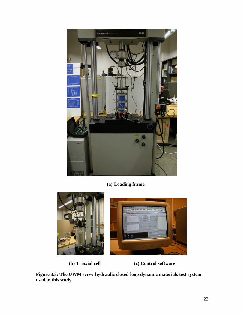
(a) Loading frame
(b) Triaxial cell (c) Control software
Figure 3.3: The UWM servo-hydraulic closed-loop dynamic materials test system
used in this study
22

Specimen Preparation
Compacted soil specimens were prepared according to the procedure described by
AASHTO T 307, which requires five-lift static compaction. Therefore, special molds
were designed and used to prepare soil specimens by static compaction of five equal
layers. This compaction method provided uniform compacted lifts while using the same
weight of soil for each lift. Figure 3.4 depicts pictures of the molds used to prepare soil
specimens and pictures of specimen preparation procedure. The molds were made in
three different diameters: 101.6, 71.1, and 35.6 mm (4.0, 2.8, and 1.4 in.).
For each soil type, compacted soil specimens were prepared at three different unit
weight-moisture content combinations, namely: maximum dry unit weight and optimum
moisture content, 95% of the maximum dry unit weight and the corresponding moisture
content on the dry side, and 95% of the maximum dry unit weight and the corresponding
moisture content on the wet side, as depicted in Figure 3.5. In order to ensure the
repeatability of test results, a special study was conducted on soil specimens prepared
under identical conditions of moisture content and unit weight. Statistical analysis was
performed on the test results to evaluate the test repeatability. Thereafter, a repeated load
triaxial test was performed on two specimens of each soil at the specified unit weight and
moisture content.
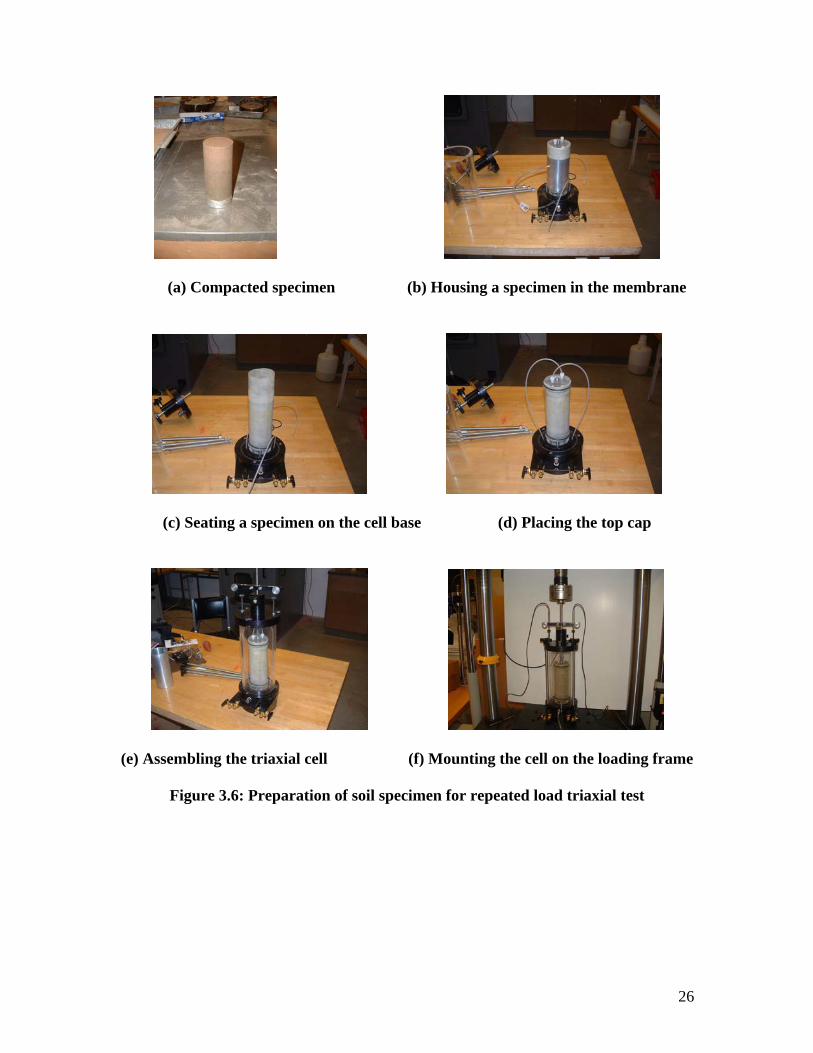
After a soil specimen was prepared under a specified unit weight and moisture content, it
was placed in a membrane and mounted on the base of the triaxial cell. Porous stones
were placed at the top and bottom of the specimen. The triaxial cell was sealed and
mounted on the base of the dynamic materials test system frame. All connections were
tightened and checked. Cell pressure, LVTD’s, load cell, and all other required setup
were connected and checked. Figure 3.6 shows pictures of specimen preparation for the
repeated load triaxial test.
Specimen Testing
The software that controls the materials dynamic test system was programmed to apply
repeated loads according to the test sequences specified by AASHTO T 307 based on the
material type. Once the triaxial cell is mounted on the system, the air pressure panel is
connected to the cell. The required confining pressure (Vc) is then applied. Figure 3.7
shows pictures of the software used to control and run the repeated load triaxial test.
The soil specimen was conditioned by applying 1,000 repetitions of a specified deviator
stress (Vd) at a certain confining pressure. Conditioning eliminates the effects of
specimen disturbance from compaction and specimen preparation procedures and
minimizes the imperfect contacts between end platens and the specimen. The specimen is
then subjected to different deviator stress sequences according to AASHTO T 307. The
23

(a) Molds of different sizes (b) Lubricating the mold
(c) Filling mold with one soil layer (d) Placing compaction piston
(e) Applying static force (f) Extracting compacted specimen
Figure 3.4: Special mold designed to prepare soil specimens according to AASHTO
T 307 requirements
24

Dry
un
it w
eig
ht,
J
d (l
b/f
t3 )
Wet side
Dry side
Maximum dry unit weight, Jdmax
1 2 30.95Jdmax
Opti
mu
m m
ois
ture
co
nte
nt,
w o
pt
Moisture content, w (%)
Figure 3.5: Conditions of unit weight and moisture content under which soil
specimens were subjected to repeated load triaxial test
stress sequence is selected to cover the expected in-service range that a pavement or
subgrade material experiences because of traffic loading.
It is very difficult to apply the exact specified loading on a soil specimen in a repeated
load configuration. This is in part due to the controls of the equipment and soil specimen
stiffness. However, the closed-loop servo hydraulic system is one of the most accurate
systems used to apply repeated loads. In this system, the applied loads and measured
displacements are continuously monitored. This is to make sure that the applied loads are
within an acceptable tolerance. If there are out of range applied loads or measured
displacements, then the system will display warning messages and can be programmed to
terminate the test.
25
(a) Compacted specimen (b) Housing a specimen in the membrane
(c) Seating a specimen on the cell base (d) Placing the top cap
(e) Assembling the triaxial cell (f) Mounting the cell on the loading frame
Figure 3.6: Preparation of soil specimen for repeated load triaxial test
26
Figure 3.7: Computer program used to control and run the repeated load triaxial
test for determination of resilient modulus
27

Chapter 4
Test Results and Analysis
This chapter presents the results of the laboratory testing program, analyses and
evaluation of test results, and statistical analysis to develop resilient modulus prediction
models. Physical and compaction properties of the investigated soils are presented and
evaluated. In addition, the results of the repeated load triaxial test to evaluate the resilient
modulus of the investigated soils are discussed. Statistical analyses are conducted to
develop correlations for predicting the resilient modulus model parameters from basic
soil properties. A critical evaluation and validation of the proposed correlations and
discussion of the results are also presented.
4.1 Properties of the Investigated Soils
Evaluation of soil properties and identification and classification of the investigated soils
are important steps to accomplish the research objective since the resilient modulus is
highly influenced by soil properties. The investigated soils comprise common types that
occur in Wisconsin. The results of laboratory tests conducted to evaluate soil properties
are presented in Table 4.1. Soil names in Table 1 are described according to the Soil
Conservation Services (SCS). The soil horizon designation is for the depth at which the
soil sample was obtained. The data on soil properties consists of particle size analysis
(sieve and hydrometer); consistency limits (LL, PL, and PI); specific gravity; maximum
dry unit weight and optimum moisture content; soil classification using the Unified Soil
Classification System (USCS); and soil classification using the AASHTO method
including group index (GI). The following is a brief description of selected soils.
Dodgeville Soil (B) Test results indicated that the soil consists of 97% of fine materials (passing sieve #200)
with a plasticity index PI = 12, which was classified as lean clay (CL) according to the
USCS and clayey soil (A-6) according to the AASHTO soil classification with a group
index GI = 13. Figure 4.1 shows the particle size distribution curve of Dodgeville soil.
The results of the Standard Proctor test on Dodgeville soil are depicted in Figure 4.2.
Results of test #1 showed that the maximum dry unit weight Jdmax =15.9 kN/m3 and the
optimum moisture content wopt. = 19.6%, while results of test #2 indicated that Jdmax =
16.25 kN/m3 and wopt. = 18.0 %. The results of the compaction tests are considered
consistent.
Antigo Soil (B) Figure 4.3 depicts the particle size distribution curve of Antigo soil. This soil consists of
91% passing sieve #200 with plasticity index PI = 11, which was classified as lean clay
(CL) according to USCS and clayey soil (A-6) according to the AASHTO soil
classification with GI=9. Standard Proctor test results showed that the average maximum
dry unit weight Jdmax = 17.5 kN/m3 and the corresponding average optimum moisture
content wopt. = 14.5%, as shown in Figure 4.4.
28
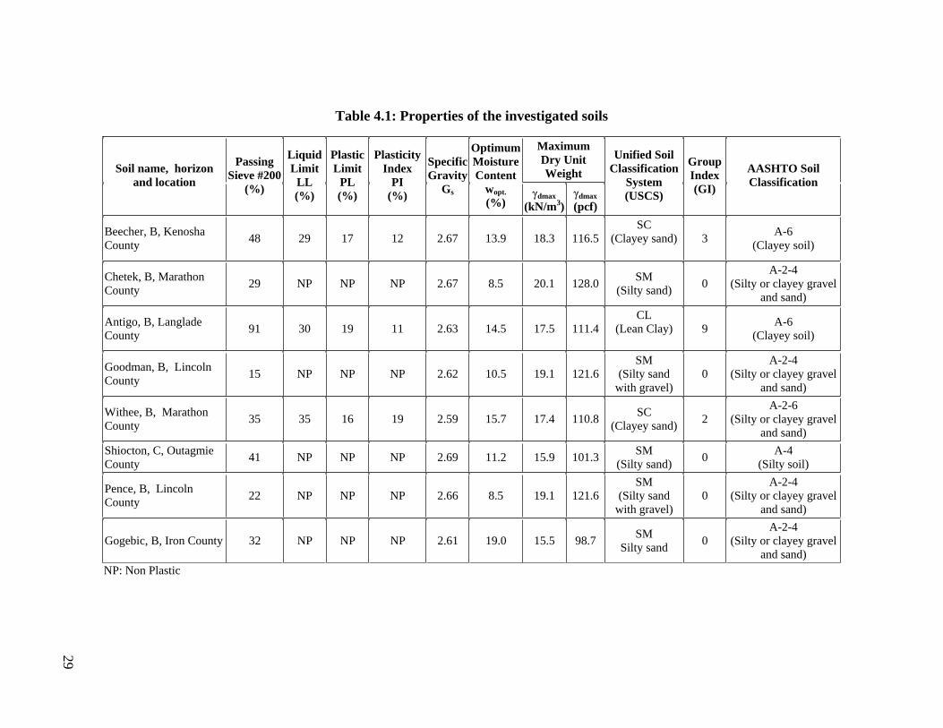
Table 4.1: Properties of the investigated soils
Soil name, horizon
and location
Passing
Sieve #200
(%)
Liquid
Limit
LL
(%)
Plastic
Limit
PL
(%)
Plasticity
Index
PI
(%)
Specific
Gravity
Gs
Optimum
Moisture
Content
wopt.
(%)
Maximum
Dry Unit
Weight
Unified Soil
Classification
System
(USCS)
Group
Index
(GI)
AASHTO Soil
Classification Jdmax
(kN/m3)
Jdmax
(pcf)
Beecher, B, Kenosha
County 48 29 17 12 2.67 13.9 18.3 116.5
SC
(Clayey sand) 3 A-6
(Clayey soil)
Chetek, B, Marathon
County 29 NP NP NP 2.67 8.5 20.1 128.0
SM
(Silty sand) 0
A-2-4
(Silty or clayey gravel
and sand)
Antigo, B, Langlade
County 91 30 19 11 2.63 14.5 17.5 111.4
CL
(Lean Clay) 9 A-6
(Clayey soil)
Goodman, B, Lincoln
County 15 NP NP NP 2.62 10.5 19.1 121.6
SM
(Silty sand
with gravel)
0
A-2-4
(Silty or clayey gravel
and sand)
Withee, B, Marathon
County 35 35 16 19 2.59 15.7 17.4 110.8
SC
(Clayey sand) 2
A-2-6
(Silty or clayey gravel
and sand)
Shiocton, C, Outagmie
County 41 NP NP NP 2.69 11.2 15.9 101.3
SM
(Silty sand) 0
A-4
(Silty soil)
Pence, B, Lincoln
County 22 NP NP NP 2.66 8.5 19.1 121.6
SM
(Silty sand
with gravel)
0
A-2-4
(Silty or clayey gravel
and sand)
Gogebic, B, Iron County 32 NP NP NP 2.61 19.0 15.5 98.7 SM
Silty sand 0
A-2-4
(Silty or clayey gravel
and sand)
NP: Non Plastic
29

Table 4.1 (cont.): Properties of the investigated soils
Soil name, horizon
Passing
Sieve Liquid Limit
LL
Plastic
Limit
Plasticity
Index Specific
Gravity
Optimum
Moisture
Content
Maximum
Dry Unit
Weight
Unified Soil
Classification
System
(USCS)
Group
Index
(GI)
AASHTO Soil
Classification and location #200
(%) (%)
PL
(%)
PI
(%) Gs wopt.
(%) Jdmax
(kN/m3)
Jdmax
(pcf)
Dodgeville, B,
Iowa County 97 37 25 12 2.55 18.8 16.1 102.5
CL
(Lean clay) 13 A-6
(Clayey soil)
Miami, B, Dodge
County 96 39 22 17 2.57 18.1 16.6 105.7
CL
(Lean clay) 18 A-6
(Clayey soil)
Ontonagon - 1, C
Ashland County 31 42 20 22 2.63 17.5 17.5 111.4
SC
(Clayey sand) 2
A-2-7
(Silty or clayey
sand and gravel)
Ontonagon - 2, C
Ashland County 26 47 22 25 2.64 22.0 16.0 101.9
SC
(Clayey sand) 2
A-2-7
(Silty or clayey
sand and gravel)
Plainfield, C, Wood
County 2 NP NP NP 2.65 - - -
SP
(Poorly graded
sand)
0 A-3
(Fine sand)
Plano, C Dane
County 27 NP NP NP 2.66 7.8 20.5 130.5
SM
(Silty sand) 0
A-2-4
(Silty or clayey
sand and gravel)
Kewaunee - 1, C
Winnebago County 30 NP NP NP 2.64 12.7 18.2 115.9
SM
(Silty sand) 0
A-2-4
(Silty or clayey
sand and gravel)
Kewaunee - 2, C
Winnebago County 48 28 14 14 2.69 13.5 19.0 121.0
SC
(Clayey sand) 3 A-6
(Clayey soil)
NP: Non plastic
30

Table 4.1 (cont.): Properties of the investigated soils
Soil name,
horizon and
location
Passing
Sieve
#200
(%)
Liquid Limit
LL
(%)
Plastic
Limit
PL
(%)
Plasticity
Index
PI
(%)
Specific
Gravity
Gs
Optimum
Moisture
Content
wopt.
(%)
Maximum
Dry Unit
Weight
Unified Soil
Classification
System
(USCS)
Group
Index
(GI)
AASHTO Soil
Classification
Jdmax
(kN/m3)
Jdmax
(pcf)
Dubuque, C, Iowa
County 72 35 23 12 2.55 18.0 16.6 105.7
CL
(Lean clay) 8
A-6
(Clayey soil)
Eleva, B,
Trempealeau
County
20 NP NP NP 2.64 7.3 20.4 129.9 SM
(Silty sand) 0
A-2-4
(Silty or clayey
gravel and sand)
Sayner-Rubicon,
C, Vilas County 1 NP NP NP 2.65 - - -
SP
(Poorly graded
sand with
gravel)
0
A-1
(Stone fragments,
gravel and sand)
NP: Non plastic
Soil name,
horizon and emax
e
min
location
Plainfield, C, 0.73 0.45
Wood County 0.68 0.44
Sayner-Rubicon,
C, Vilas County 0.71 0.45
31

Particle size (inch)
0.1 0.01 0.001 0.0001
Per
cent
fine
r (%
) 100
80
60
40
20
0
Dodgeville soil (B)
10 1 0.1 0.01 0.001
Particle size (mm)
Figure 4.1: Particle size distribution curve of Dodgeville soil (B)
13
14
15
16
17
18
Dry
uni
t wei
ght, J d
(kN
/m3 )
84 86 88 90 92 94 96 98 100 102 104 106 108 110 112 114
Dry
uni
t wei
ght, J d
(lb/ft
3 )
Dodgeville soil (B)
Test 1 Test 2
0 4 8 12 16 20 24 28 32 36 40
Moisture content, w(%)
Figure 4.2: Results of Standard Proctor test for Dodgeville soil (B)
32
Per
cent
fine
r (%
)
Particle size (inch)
1 0.1 0.01 0.001 0.0001
100
80
60
40
20
0
Antigo soil
100 10 1 0.1 0.01 0.001 Particle size (mm)
Figure 4.3: Particle size distribution curve of Antigo soil
16
17
18
19
Dry
uni
t wei
gh
t, J d
(kN
/m3 )
102
104
106
108
110
112
114
116
118
120
Dry
uni
t wei
ght, J d
(pcf
)
Antigo soil Test 1 Test 2
0 5 10 15 20 25
Moisture content, w (%)
Figure 4.4: Results of Standard Proctor test for Antigo soil
33

Plano Soil (C)
This soil consists of 27% passing sieve #200. It was classified as silty sand (SM)
according to the USCS and silty or clayey sand and gravel (A-2-4) according to the
AASHTO soil classification with GI = 0. Figure 4.5 shows the particle size distribution
curve of Plano soil. Standard Proctor test results (Figure 4.6) showed that the average
maximum dry unit weight Jdmax = 20.5 kN/m3 and the average optimum moisture content
wopt. = 7.8%.
Kewaunee Soil - 1 (C)
Test results showed that the soil consisted of 30% passing sieve #200 and was classified
as silty sand (SM) according to USCS and silty or clayey sand and gravel (A-2-4)
according to the AASHTO soil classification with GI = 0. Figure 4.7 shows the particle
size distribution curve of Kewaunee soil - 1. Figure 4.8 depicts the results of the Standard
Proctor test in which the average maximum dry unit weight Jdmax = 18.2 kN/m3 and the
corresponding average optimum moisture content wopt.= 12.7%.
The results of particle size analysis and the Standard Proctor test for the investigated soils
are presented in Appendix A. A summary of the Standard Proctor test results on the
investigated soils is presented in Table 4.2.
4.2 Resilient Modulus of the Investigated Soils
Typical results of the repeated load triaxial test conducted on the investigated soils are
shown in Table 4.3. The test was conducted on Antigo soil specimens 1 and 2 compacted
at 0.95Jdmax and moisture content w > wopt. (wet side). Table 4.3 presents the mean
resilient modulus values, standard deviation, and coefficient of variation for the 15 test
sequences conducted according to AASHTO T 307. The mean resilient modulus values,
standard deviation and coefficient of variation summarized in Table 4.3 are obtained
from the last five load cycles of each test sequence. The coefficient of variation for the
test results presented in Table 4.3 ranges between 0.14 and 1.04% for specimen #1 and
from 0.11 to 0.51% for specimen #2. This indicates that each soil specimen showed
consistent behavior during each test sequence.
Figure 4.9 shows a graphical representation of the results presented in Table 4.3.
Inspection of Figure 4.9 indicates that the resilient modulus (Mr) of Antigo clay decreases
with the increase of the deviator stress (Vd) under constant confining pressure (Vc). Under
constant Vc = 41.4 kPa, the resilient modulus decreased from Mr = 49.65 MPa at Vd =
12.45 kPa to Mr = 28.33 MPa at Vd = 59.36 kPa for Antigo soil specimen #1. Moreover,
the resilient modulus increases with the increase of confining pressure under constant
deviator stress, which reflects a typical behavior. The results presented herein are typical
resilient modulus results that are consistent with what was discussed in Chapter 2
“Background” and are significantly affected by the stress level.
34

Particle size (inch)
1 0.1 0.01 0.001 0.0001
0
20
40
60
80
100 P
erce
nt fi
ner
(%)
Plano soil
100 10 1 0.1 0.01 0.001
Particle size (mm)
Figure 4.5: Particle size distribution curve of Plano soil
17
18
19
20
21
22
Dry
uni
t wei
ght, J d
(kN
/m3 )
110 112 114 116 118 120 122 124 126 128 130 132 134 136 138
Dry
uni
t we
igh
t, J d
(pcf
)
Plano soil Test 1 Test 2
0 5 10 15 20
Moisture content, w(%)
Figure 4.6: Results of Standard Proctor test for Plano soil
35
Particle size (inch)
1 0.1 0.01 0.001 0.0001
0
20
40
60
80
100 P
erce
nt fi
ner
(%)
Kewaunee soil - 1
100 10 1 0.1 0.01 0.001
Particle size (mm)
Figure 4.7: Particle size distribution curve of Kewaunee soil - 1
15
16
17
18
19
20
Dry
uni
t wei
ght, J d
(kN
/m3 )
96 98 100 102 104 106 108 110 112 114 116 118 120 122 124 126
Dry
uni
t wei
ght, J d
(pcf
)
Kewaunee soil - 1 Test 1 Test 2
0 5 10 15 20 25
Moisture content, w(%)
Figure 4.8: Results of Standard Proctor test for Kewaunee soil - 1
36

Table 4.2: Results of the standard compaction test on the investigated soils
Soil
Test 1 Test 2 Average
Jdmax
(kN/m3)
wopt.
(%) Jdmax
(kN/m3)
wopt.
(%) Jdmax
(kN/m3)
wopt.
(%)
Antigo 17.5 14.5 17.5 14.5 17.5 14.5
Beecher 18.3 14.1 18.3 13.7 18.3 13.9
Goodman 19.1 10.5 NA NA 19.1 10.5
Plano 20.7 8.0 20.3 7.5 20.5 7.8
Dodgeville 15.9 19.6 16.2 18.0 16.1 18.8
Dubuque 16.5 18.0 16.7 18.0 16.6 18.0
Chetek 20.1 8.4 20.1 8.5 20.1 8.5
Eleva 20.2 7.5 20.7 7.1 20.4 7.3
Pence 19.1 8.5 NA NA 19.1 8.5
Gogebic 16.0 17.5 15.0 20.5 15.5 19.0
Miami 16.5 18.4 16.7 17.8 16.6 18.1
Ontonagon -1 17.5 17.5 NA NA 17.5 17.5
Ontonagon -2 16.0 22.0 NA NA 16.0 22.0
Kewaunee - 1 18.2 12.8 18.2 12.5 18.2 12.7
Kewaunee - 2 19.0 13.0 18.9 14.0 19.0 13.5
Shiocton 16.0 11.0 15.7 11.3 15.9 11.2
Withee 17.6 15.5 17.2 15.8 17.4 15.7
37

Table 4.3: Typical results of the repeated load triaxial test conducted according to
AASHTO T 307
Test
Sequence
No.
Confining
Stress
Vc (kPa)
Deviator
Stress
Vd (kPa)
Antigo wet #1
Mr (MPa) Deviator
Stress
Vd (kPa)
Antigo wet #2
Mr (MPa)
Mean SD
CV
(%) Mean SD
CV
(%)
1 41.4 12.45 49.65 0.30 0.60 12.35 57.96 0.24 0.41
2 41.4 24.91 43.30 0.45 1.04 24.92 51.74 0.14 0.28
3 41.4 36.71 36.72 0.08 0.21 36.94 44.83 0.16 0.36
4 41.4 47.90 30.55 0.08 0.25 48.11 37.13 0.07 0.19
5 41.4 59.36 28.33 0.07 0.24 59.67 34.18 0.05 0.15
6 27.6 12.29 40.79 0.17 0.43 12.24 48.69 0.19 0.39
7 27.6 23.98 30.23 0.09 0.28 24.15 38.65 0.18 0.46
8 27.6 35.51 26.00 0.09 0.34 35.82 32.97 0.11 0.33
9 27.6 48.44 24.22 0.07 0.29 47.79 29.92 0.03 0.11
10 27.6 60.25 23.31 0.03 0.14 59.80 28.28 0.04 0.15
11 13.8 12.08 30.67 0.16 0.53 12.02 37.60 0.19 0.51
12 13.8 23.37 21.42 0.05 0.24 23.83 27.92 0.13 0.46
13 13.8 35.81 18.80 0.06 0.31 35.41 23.88 0.11 0.47
14 13.8 48.43 18.57 0.04 0.20 47.53 22.44 0.05 0.22
15 13.8 60.18 18.68 0.05 0.29 59.22 21.91 0.05 0.24
SD: Standard Deviation
CV: Coefficient of Variation
38

Deviator Stress, Vd (psi)
2 4 6 8 10 200
20,000
10 100 20 40 60 80
Deviator Stress, Vd (kPa)
Vc=41.4 kPa
Vc=27.6 kPa
Vc=13.8 kPa
Antigo - Test 1 at 95% Jdmax (wet side)
Res
ilien
t Mod
ulus
, Mr (
MP
a)
Res
ilien
t Mod
ulus
, Mr (
MP
a)
100 80
Re
silie
nt M
odul
us, M
r (ps
i)
Res
ilien
t Mod
ulus
, Mr (
psi)
10,000 60 8,000
6,000
4,000
40
20
2,000
10
(a) Test on soil specimen #1
Deviator Stress, Vd (psi)
2 4 6 8 10 200
20,000
10 100 20 40 60 80
Deviator Stress, Vd (kPa)
Vc=41.4 kPa
Vc=27.6 kPa
Vc=13.8 kPa
Antigo - Test 2 at 95% Jdmax (wet side)
100 80
10,000 60 8,000
6,000
4,000
40
20
2,000
10
(b) Test on soil specimen #2
Figure 4.9: Results of repeated load triaxial test on Antigo soil compacted at 95% of
maximum dry unit weight (Jdmax) and moisture content more than wopt. (wet side)
39

A repeatability investigation was conducted to ensure that high quality test results can be
obtained. This is essential since the data will be used to develop and validate resilient
modulus correlations for use in the mechanistic-empirical pavement design. In addition,
repeated load triaxial tests were conducted on two soil specimens of each investigated
soil under identical moisture content and unit weight.
To investigate the repeatability of test results, Dodgeville soil was selected where seven
soil specimens were prepared at maximum dry unit weight and optimum moisture
content, four soil specimens were prepared at 95% of maximum dry unit weight and
moisture content less than the optimum (dry side), and two soil specimens were prepared
at 95% of maximum dry unit weight and moisture content greater than the optimum (wet
side). Repeatability test results are shown in Figures 4.10, 4.11 and 4.12, respectively.
A statistical analysis was conducted on Dodgeville soil test results to evaluate test
repeatability. Tables 4.4, 4.5, and 4.6 present the results of the analysis. Examination of
Tables 4.4-4.6 indicates that the deviator stress applied by the system was accurate with
coefficient of variation CV(Vd) ranges from 0 to 4.4%. The coefficient of variation for the
resilient modulus CV(Mr) varies from 0.2 to 2.9% for the maximum dry unit weight
specimens, between 5.1 and 13.2% for the 95% of maximum dry unit weight specimens
(dry side), and from 1.8 to 20.2% for the 95% of maximum dry unit weight specimens
(wet side). The best repeatability results were obtained for the specimens compacted at
the maximum dry unit weight and optimum moisture content. Based on this repeatability
analysis, the test results are considered consistent and repeatable.
Figure 4.13 presents the results of the repeated load triaxial test on Antigo and
Dodgeville soils compacted at maximum dry unit weight and optimum moisture content.
Test results on Antigo soil (Figure 4.13a) showed that at confining pressure Vc = 41.4
kPa, the resilient modulus decreased from Mr = 94 MPa at Vd = 12.6 kPa to Mr = 81 MPa
at Vd = 61.5 kPa. For Dodgeville soil (Figure 4.13b) and under the same confining
pressure, the resilient modulus decreased from Mr = 75 MPa at Vd = 12.4 kPa to Mr = 59
MPa at Vd = 60.6 kPa. Both soils showed that Mr is decreasing with the increase in the
deviator stress; however, Antigo soil exhibited higher resilient modulus values compared
to Dodgeville soil. This is attributed to the higher maximum dry unit weight and lower
moisture content values of the Antigo specimen compared to the Dodgeville specimen.
The Antigo soil specimen #1 (Figure 4.13a) was subjected to the repeated load triaxial
test at Jdmax = 17.4 kN/m3 and wopt. = 14.6%, while the Dodgeville specimen #5 was tested
at Jdmax = 15.8 kN/m3 and wopt. = 20.1%. The resilient modulus as a dynamic soil stiffness
modulus is affected by moisture content and unit weight of the soil. Soils under higher
unit weight and lower moisture content are expected to show higher stiffness modulus.
Figure 4.14 presents the results of the repeated load triaxial test on Beecher soil at 95%
Jdmax and w < wopt, at Jdmax and wopt, and at 95% Jdmax and w > wopt. This is to demonstrate
the effect of the moisture content on the resilient modulus of the investigated soils. Test
results on the Beecher soil specimen tested at 95% Jdmax and w < wopt (dry side) showed
that
40

Deviator Stress, Vd (psi)
2 4 6 8 10
10
100
20
40
60
80
200
Res
ilien
t Mod
ulus
, Mr (
MP
a)
10,000
20,000
8,000
6,000
4,000
2,000
Re
silie
nt M
odul
us, M
r (ps
i)
Vc=41.4 kPa
Vc=27.6 kPa
Vc=13.8 kPa
Dodgeville - Test 3 at Jdmax and wopt.
10 20 40 60 80 100
Deviator Stress, Vd (kPa)
(a) Test on soil specimen #3
Deviator Stress, Vd (psi)
2 4 6 8 10
10 100 20 40 60 80
Deviator Stress, Vd (kPa)
10
100
20
40
60
80
200
Re
silie
nt M
odu
lus,
Mr (
MP
a)
10,000
20,000
8,000
6,000
4,000
2,000
Re
silie
nt M
odul
us, M
r (ps
i)
Vc=41.4 kPa
Vc=27.6 kPa
Vc=13.8 kPa
Dodgeville - Test 5 at Jdmax and wopt.
(b) Test on soil specimen #5
Figure 4.10: Results of repeated load triaxial test on Dodgeville soil compacted at
maximum dry unit weight (Jdmax) and optimum moisture content (wopt.)
41

Deviator Stress, Vd (psi)
2 4 6 8 10
10
100
20
40
60
80
200
Res
ilien
t Mod
ulus
, Mr (
MP
a)
10,000
20,000
8,000
6,000
4,000
2,000
Re
silie
nt M
odul
us, M
r (ps
i)
Vc=41.4 kPa
Vc=27.6 kPa
Vc=13.8 kPa
Dodgeville - Test 6 at Jdmax and wopt.
10 20 40 60 80 100
Deviator Stress, Vd (kPa)
(c) Test on soil specimen #6
Deviator Stress, Vd (psi)
2 4 6 8 10
10 100 20 40 60 80
Deviator Stress, Vd (kPa)
10
100
20
40
60
80
200
Res
ilien
t Mod
ulus
, Mr (
MP
a)
10,000
20,000
8,000
6,000
4,000
2,000
Re
silie
nt M
odul
us, M
r (ps
i)
Vc=41.4 kPa
Vc=27.6 kPa
Vc=13.8 kPa
Dodgeville - Test 7 at Jdmax and wopt.
(d) Test on soil specimen #7
Figure 4.10 (cont.): Results of repeated load triaxial test on Dodgeville soil
compacted at maximum dry unit weight (Jdmax) and optimum moisture content (wopt.)
42

Deviator Stress, Vd (psi)
2 4 6 8 10
10
100
20
40
60
80
200
Res
ilien
t Mod
ulus
, Mr (
MP
a)
10,000
20,000
8,000
6,000
4,000
2,000
Res
ilien
t Mod
ulus
, Mr (
psi)
Vc=41.4 kPa
Vc=27.6 kPa
Vc=13.8 kPa
Dodgeville - Test 1 at 95% Jdmax (dry side)
10 20 40 60 80 100
Deviator Stress, Vd (kPa)
(a) Test on soil specimen #1
Deviator Stress, Vd (psi)
2 4 6 8 10
10 100 20 40 60 80
Deviator Stress, Vd (kPa)
10
100
20
40
60
80
200
Res
ilien
t Mod
ulus
, Mr (
MP
a)
10,000
20,000
8,000
6,000
4,000
2,000
Re
silie
nt M
odul
us, M
r (ps
i)
Vc=41.4 kPa
Vc=27.6 kPa
Vc=13.8 kPa
Dodgeville - Test 2 at 95% Jdmax (dry side)
(b) Test on soil specimen #2
Figure 4.11: Results of repeated load triaxial test on Dodgeville soil compacted at
95% of maximum dry unit weight (Jdmax) and moisture content less than wopt. (dry
side)
43

Deviator Stress, Vd (psi)
2 4 6 8 10
10
100
20
40
60
80
200
Res
ilien
t Mod
ulus
, Mr (
MP
a)
10,000
20,000
8,000
6,000
4,000
2,000
Re
silie
nt M
odul
us, M
r (ps
i)
Vc=41.4 kPa
Vc=27.6 kPa
Vc=13.8 kPa
Dodgeville - Test 3 at 95% Jdmax (dry side)
Res
ilien
t Mod
ulus
, Mr (
MP
a)
10 20 40 60 80 100
Deviator Stress, Vd (kPa)
(c) Test on soil specimen #3
Deviator Stress, Vd (psi)
2 4 6 8 10 200
20,000
100 80
10,000 60 8,000
10 100 20 40 60 80
Deviator Stress, Vd (kPa)
6,000
4,000
2,000
Vc=41.4 kPa
Vc=27.6 kPa
Vc=13.8 kPa
Dodgeville - Test 4 at 95% Jdmax (dry side)
40
20
Re
silie
nt M
odul
us, M
r (ps
i)
10
(d) Test on soil specimen #4
Figure 4.11 (cont.): Results of repeated load triaxial test on Dodgeville soil
compacted at 95% of maximum dry unit weight (Jdmax) and moisture content less
than wopt. (dry side)
44

Deviator Stress, Vd (psi)
2 4 6 8 10 100
80
10 100 20 40 60 80
Deviator Stress, Vd (kPa)
Vc=41.4 kPa
Vc=27.6 kPa
Vc=13.8 kPa
Dodgeville - Test 1 at 95% Jdmax (wet side)
10,000 60 8,000
Res
ilien
t Mod
ulus
, Mr (
MP
a)
Res
ilien
t Mod
ulus
, Mr (
MP
a)
Re
silie
nt M
odul
us, M
r (ps
i)
Re
silie
nt M
odul
us, M
r (ps
i)
6,000 40 4,000
20 2,000
10 8 1,000 6 800
600 4 400
2 200
1
(a) Test on soil specimen #1
Deviator Stress,Vd (psi)
2 4 6 8 10 100
80
10 100 20 40 60 80
Deviator Stress,Vd (kPa)
Vc=41.4 kPa
Vc=27.6 kPa
Vc=13.8 kPa
Dodgeville - Test 2 at 95% Jdmax (wet side)
10,000 60 8,000 6,000 40 4,000
20 2,000
10 8 1,000 6 800
600 4 400
2 200
1
(b) Test on soil specimen #2
Figure 4.12: Results of repeated load triaxial test on Dodgeville soil compacted at
95% of maximum dry unit weight (Jdmax) and moisture content more than wopt. (wet
side)
45

Table 4.4: Analysis of repeatability tests on Dodgeville soil tested at maximum dry unit weight and optimum moisture content
Test
Sequence Vc
(kPa)
Test #5 Test #6 Test #7 Mean
Vd
(kPa)
Mean
Mr
(MPa) CV(Vd) CV(Mr)Vd
(kPa)
Mr
(MPa) Vd
(kPa)
Mr
(MPa) Vd
(kPa)
Mr
(MPa)
1 12.4 75.0 12.8 76.0 12.5 76.9 12.6 76.0 1.6 1.2
2 24.7 73.1 25.1 73.1 24.9 72.7 24.9 73.0 0.8 0.3
3 41.4 37.3 71.1 37.7 68.7 37.2 68.3 37.4 69.4 0.8 2.2
4 49.2 65.3 49.7 61.8 49.0 62.7 49.3 63.3 0.7 2.9
5 60.6 58.8 61.4 55.5 60.4 56.9 60.8 57.1 0.8 2.9
6 12.4 69.7 12.7 70.6 12.4 70.7 12.5 70.3 1.5 0.8
7 24.5 65.1 24.9 63.1 24.5 63.7 24.6 64.0 0.9 1.6
8 27.6 36.6 60.5 37.2 58.1 36.6 58.8 36.8 59.1 0.9 2.1
9 48.5 56.8 49.2 53.9 48.3 54.9 48.7 55.2 1.0 2.6
10 60.1 53.3 60.9 50.3 60.0 51.8 60.3 51.8 0.8 2.9
11 12.2 62.1 12.6 62.4 12.3 62.3 12.4 62.3 1.6 0.2
12 24.3 55.5 24.6 54.2 24.2 54.5 24.3 54.7 0.8 1.3
13 13.8 36.1 51.6 36.5 49.7 35.9 50.1 36.2 50.5 0.9 1.9
14 47.6 48.5 48.5 46.4 47.4 47.1 47.8 47.3 1.2 2.2
15 59.2 46.0 60.2 43.7 58.9 45.3 59.5 45.0 1.1 2.7
46

Table 4.5: Analysis of repeatability tests on Dodgeville soil tested at 95% of maximum dry unit weight and moisture content
less than the optimum moisture content (dry side)
Test
Sequence Vc
(kPa)
Test #1 Test #2 Test #4 Mean
Vd
(kPa)
Mean
Mr
(MPa) CV(Vd) CV(Mr)Vd
(kPa)
Mr
(MPa) Vd
(kPa)
Mr
(MPa) Vd
(kPa)
Mr
(MPa)
1 12.8 109.2 11.9 130.3 12.8 142.3 12.5 127.3 4.4 13.2
2 25.2 126.8 25.4 133.5 25.5 146.4 25.4 135.6 0.5 7.3
3 41.4 37.7 133.6 37.6 133.3 38.0 146.5 37.8 137.8 0.6 5.5
4 50.5 133.5 49.7 133.7 50.5 145.7 50.2 137.6 0.9 5.1
5 62.7 131.6 62.2 131.0 63.1 145.3 62.7 136.0 0.7 6.0
6 12.8 105.0 11.7 125.1 12.2 134.9 12.2 121.7 4.4 12.5
7 25.3 118.7 25.0 126.1 25.3 138.9 25.2 127.9 0.7 8.0
8 27.6 37.8 125.1 37.4 125.7 37.7 138.5 37.6 129.8 0.5 5.8
9 50.2 127.1 49.6 124.2 50.3 138.4 50.0 129.9 0.7 5.8
10 62.6 126.8 62.1 123.2 63.3 138.8 62.7 129.6 1.0 6.3
11 12.4 99.5 11.8 110.8 12.0 123.8 12.1 111.4 2.8 10.9
12 25.0 104.6 24.7 112.4 25.2 126.7 25.0 114.6 1.0 9.8
13 13.8 37.3 109.8 37.1 112.2 37.5 127.3 37.3 116.4 0.6 8.2
14 50.0 113.0 49.4 111.7 50.2 127.7 49.9 117.5 0.8 7.5
15 62.4 114.5 61.9 111.5 63.1 128.8 62.5 118.3 1.0 7.8
47

Table 4.6: Analysis of repeatability tests on Dodgeville soil tested at 95% of maximum dry unit weight and moisture content
greater than the optimum moisture content (wet side)
Test
Sequence Vc
(kPa)
Test #1 Test #2 Mean
Vd
(kPa)
Mean
Mr
(MPa) CV(Vd) CV(Mr)Vd
(kPa)
Mr
(MPa) Vd
(kPa)
Mr
(MPa)
1 12.6 33.7 12.3 25.3 12.5 29.5 1.4 20.2
2 24.5 24.3 24.5 19.5 24.5 21.9 0.2 15.5
3 41.4 36.6 20.4 35.9 15.5 36.2 17.9 1.2 19.1
4 48.2 17.1 47.3 13.2 47.8 15.2 1.2 18.1
5 59.7 14.9 59.2 13.0 59.5 13.9 0.5 9.5
6 12.0 19.1 12.1 16.7 12.0 17.9 0.2 9.4
7 23.4 13.1 23.6 12.3 23.5 12.7 0.8 4.4
8 27.6 35.5 12.3 36.0 12.0 35.8 12.2 1.0 1.8
9 48.0 12.8 48.3 12.2 48.1 12.5 0.4 3.5
10 59.9 13.2 60.0 12.3 59.9 12.7 0.1 4.9
11 11.9 15.0 11.9 12.8 11.9 13.9 0.0 11.1
12 22.7 10.1 23.5 9.4 23.1 9.7 2.4 5.0
13 13.8 35.1 10.1 36.0 9.4 35.6 9.7 1.9 4.7
14 47.8 11.0 48.5 10.2 48.2 10.6 1.1 5.3
15 59.8 11.9 60.7 11.0 60.3 11.4 1.0 5.6
48
Deviator Stress, Vd (psi)
2 4 6 8 10 200
20,000
10 100 20 40 60 80
Deviator Stress, Vd (kPa)
Vc=41.4 kPa
Vc=27.6 kPa
Vc=13.8 kPa
Antigo - Test 1 at Jdmax = 17.4 kN/m3 and wopt. = 14.6%
Re
silie
nt M
odu
lus,
Mr (
MP
a)
Res
ilien
t Mod
ulus
, Mr (
MP
a)
100 80
10,000 60 8,000
6,000 40
Re
silie
nt M
odul
us, M
r (ps
i)
Res
ilien
t Mod
ulus
, Mr (
psi)
4,000
20
2,000
10
(a) Antigo
Deviator Stress, Vd (psi)
2 4 6 8 10 200
20,000
10 100 20 40 60 80
Deviator Stress, Vd (kPa)
Vc=41.4 kPa
Vc=27.6 kPa
Vc=13.8 kPa
Dodgeville - Test 5 at Jdmax= 15.8 kN/m3 and wopt.= 20.1%
100 80
10,000 60 8,000
6,000 40
4,000
20
2,000
10
(b) Dodgeville
Figure 4.13: The effect of unit weight and moisture content on the resilient modulus
of the investigated soils
49

Deviator Stress, Vd (psi) Deviator Stress, Vd (psi)
2 4 6 8 10 2 4 6 8 10 200 200
20,000
10 10020 40 60 80
Deviator Stress, Vd (kPa)
Vc=41.4 kPa
Vc=27.6 kPa
Vc=13.8 kPa
Beecher - Test 2 at 95% Jdmax (dry side)
Jd = 17.3 kN/m3 and w . = 10%
20,000
10 10020 40 60 80
Deviator Stress, Vd (kPa)
Vc=41.4 kPa
Vc=27.6 kPa
Vc=13.8 kPa
Beecher - Test 1 at Jdmax= 18.3 kN/m3 and wopt.= 14%
Res
ilien
t Mod
ulus
, Mr (
MP
a)
Res
ilien
t Mo
dulu
s, M
r (p
si)
Res
ilien
t Mod
ulus
, Mr (
MP
a)
Re
silie
nt M
od
ulus
, Mr (
psi
)
100 80
100 80
10,000 10,000 60 608,000 8,000
6,000 6,000 40 40
4,000 4,000
20 20
2,000 2,000
10 10
(a) Dry side (b) Optimum
Deviator Stress, Vd (psi)
2 4 6 8 10 200
20,000
10 10020 40 60 80
Deviator Stress, Vd (kPa)
Vc=41.4 kPa
Vc=27.6 kPa
Vc=13.8 kPa
Beecher - Test 1 at 95% Jdmax (wet side)
at Jd = 17.3 kN/m3 and w = 16.3%
Res
ilien
t Mod
ulus
, Mr (
MP
a)
Res
ilien
t Mod
ulus
, Mr (
psi
)
100 80
10,000 60 8,000
6,000
4,000
40
20
2,000
10
(c) Wet side
Figure 4.14: The effect of the moisture content on the resilient modulus of the
investigated soils
50

at confining pressure Vc = 41.4 kPa, the resilient modulus decreased from Mr = 119 MPa
at Vd = 12.5 kPa to Mr = 114 MPa at Vd = 60.7 kPa. The Beecher specimen tested at 95%
Jdmax and w > wopt showed a decrease in the resilient modulus from Mr = 72 MPa at Vd =
13.6 kPa to Mr = 42 MPa at Vd = 60.3 kPa. Both specimens have similar unit weight
values (Jd = 17.3 kN/m3) and different moisture content. The Beecher specimen with
lower moisture content exhibited higher resilient modulus values compared to the other
specimen with higher moisture content under the same unit weight. The effect of
increased moisture content of the soil on reducing the resilient modulus is significant.
The soil specimen tested at Jdmax and wopt exhibited resilient modulus values less than the
specimen compacted at 95% Jdmax and w < wopt (dry side). This is mainly attributed to the
moisture content since the specimen compacted at optimum moisture content has 4%
more moisture. Even though the specimen compacted at Jdmax has higher unit weight, the
influence of moisture content surpassed the effect of unit weight.
For many of the investigated soils, the resilient modulus values of the soil compacted at
95%Jdmax on the dry side are higher than Mr values of the same soil compacted at Jdmax and
optimum moisture content. The soil compacted at moisture content less than the optimum
and 95%Jdmax exhibited hardening and showed higher values of resilient modulus with the
increase of the deviator stress. The soil compacted at unit weight of 95% Jdmax on the wet
side exhibited low resilient modulus values compared to the same soil compacted at
optimum moisture content.
The results of repeated load triaxial test on the investigated soils are presented in
Appendix B.
4.3 Statistical Analysis
Results obtained from basic soil testing and repeated load triaxial test were used to
develop correlations for predicting the resilient modulus model parameters using the
resilient modulus constitutive equation selected by NCHRP Project 1-37A for the
mechanistic-empirical pavement design. Repeated load triaxial tests were conducted, on
average, six times on each soil type at three different moisture content levels and two dry
unit weight levels (i.e. 95% Jdmax and Jdmax). It should be noted that Kewaunee soil was
subjected to testing only once under each moisture content level due to unavailability of
soil samples.
4.3.1 Evaluation of the Resilient Modulus Model Parameters
The resilient modulus model is a general constitutive equation that was developed
through NCHRP project 1-28A and was selected for implementation in the upcoming
AASHTO Guide for the Design of New and Rehabilitated Pavement Structures. The
resilient modulus model can be used for all types of subgrade materials. The resilient
modulus model is defined by (NCHRP 1-28A):
51

§V · k2 §W ·
k3
b octM r k1Pa ̈̈ ¸̧ ¨̈ �1¸ (4.1) ¸P P© a ¹ © a ¹ where:
Mr = resilient modulus
Pa = atmospheric pressure (101.325 kPa)
Vb = bulk stress = V1 + V2+ V3
V1 = major principal stress
V2 = intermediate principal stress = V3 in axisymmetric condition (triaxial test)
V3 = minor principal stress or confining pressure in the repeated load triaxial test
Woct = octahedral shear stress
k1, k2 and k3 = material model parameters
The octahedral shear stress is defined in general as:
1 2 2 2W (V �V ) � (V �V ) � (V �V ) (4.2)oct 1 2 1 3 2 33
For axisymmetric stress condition (triaxial), V2 = V3 and V1 - V3 = Vd (deviator stress),
therefore the octahedral shear stress is reduced to:
W 2 �V � (4.3)oct d3
The resilient modulus, the bulk stress and the octahedral shear stress are normalized in
this model by the atmospheric pressure. This will result in non-dimensional model
parameters.
Statistical analysis based on multiple linear regression was utilized to determine the
resilient modulus model parameters k1, k2 and k3. The statistical analysis software
STATISTICA was used to perform the analysis. In order to determine k1, k2, and k3 using
the experimental test results, the resilient modulus model Equation 4.1 was transformed
to:
§ M · §V · §W · r b octlog¨ ¸ log k1 � k2 log¨ ¸ � k3 log¨ �1¸ (4.4)¨ ¸ ¨ ¸ ¨ ¸P P P© a ¹ © a ¹ © a ¹
The resilient modulus is treated as the dependent variable, while bulk and octahedral
shear stresses are used as the independent variables. The analysis was carried out for each
soil type to evaluate the model parameters (k1, k2 and k3) from the results of the 15 stress
combinations applied during repeated load triaxial test (15 load sequences according to
AASHTO T 307). A total of 136 repeated load tests were used in the analysis. Results of
this analysis are summarized in Table 4.7.
52

Table 4.7: Basic statistical data of the resilient modulus model parameters ki
obtained from the test results of the investigated soils
Parameter Mean Median Minimum Maximum Std. Dev. Standard
Error
k1 826.8 832.0 201.2 1318.7 250.4 21.47
k2 0.517 0.456 0.176 1.083 0.243 0.021
k3 -2.142 -1.919 -6.013 -0.105 1.373 0.118
The analysis showed that k1 ranges from 201.2 to 1318.7 with a mean value of 826.8. The
magnitude of k1 was always > 0 since the resilient modulus should always be greater than
zero. The parameter k2 which, is related to the bulk stress, varies between 0.176 and
1.083 with mean value of 0.517. The values of k2 were also greater than zero since the
resilient modulus increases with the increase in the bulk stress (confinement). Since the
resilient modulus decreases with the increase in the deviator stress, the parameter k3
ranges from -6.013 to -0.105 with a mean value of -2.142. The model parameters ki
obtained from the statistical analysis on the repeated load test results are presented in
histograms in Figure 4.15.
4.3.2 Correlations of Model Parameters with Soil Properties
The resilient modulus model parameters k1, k2 and k3 were determined for all soil types.
These parameters are then correlated to fundamental soil properties using regression
analysis. The values of resilient modulus model parameters (k1, k2 and k3) were
alternatively used as dependent variables while various fundamental soil properties were
treated as independent variables. Various combinations of soil properties (independent
variables) were used in the regression analysis. The general multiple linear regression
model is expressed as:
k E � E x � E x � � � � � E x �� (4.5)i 0 1 1 2 2 k k
where:
ki = the dependent variable for the regression, (model parameters k1, k2 or k3)
E0 = intercept of the regression plane
Ei = regression coefficient
xi = the independent or regressor variable, (in this study, soil property or a
combination of soil properties)
� = random error
It should be noted that general nonlinear models that include factorial and polynomial
regression were attempted in this study. The resulted correlations were not successful due
to the existence of a large intercorrelation between the independent variables. In addition,
some of the correlation coefficients conflict with the natural behavior of soils. As an
example, the increase in the dry unit weight leads to a decrease in the resilient modulus.
53
0
2
4
6
8
10
12
14
16
No.
of o
bser
vatio
ns
201 335 469 604 738 872 1006 1140 1274
k1
(a) Resilient modulus model parameter k1
0
2
4
6
8
10
12
14
16
No.
of o
bser
vatio
ns
0.177 0.285 0.394 0.503 0.612 0.720 0.829 0.938 1.047
k2
(b) Resilient modulus model parameter k2
Figure 4.15: Histograms of resilient modulus model parameters ki obtained from
statistical analysis on the results of the investigated Wisconsin soils
54

No.
of o
bser
vatio
ns
18
16
14
12
10
8
6
4
2
0 -6.01 -5.30 -4.60 -3.89 -3.18 -2.47 -1.76 -1.05 -0.34
k3
(c) Resilient modulus model parameter k3
Figure 4.15 (cont.): Histograms of resilient modulus model parameters ki obtained
from statistical analysis on the results of the investigated Wisconsin soils
Selection of Soil Properties
The resilient modulus is used to evaluate the stiffness of bound/unbound materials.
Factors that affect resilient modulus are stress state, soil type and the environmental
conditions of the soil that influence the soil physical state (unit weight and moisture
content). Stress state is expressed in the resilient modulus model by including bulk and
octahedral stresses. The soil type and the current soil physical condition should be
included in attempted correlations in order to obtain valid estimation/prediction of the
resilient modulus.
Sets of independent variables are specified to reflect soil type and current soil physical
condition. Independent variables available from basic soil testing that represent soil type
and current soil physical condition are: percent passing sieve #4 (PNo.4), percent passing
sieve #40 (PNo.40), percent passing sieve #200 (PNo.200), liquid limit (LL), plastic limit
(PL), Plasticity Index (PI), Liquidity Index (LI), amount of sand (%Sand), amount of silt
(%Silt), amount of clay (%Clay), water content (w) and dry unit weight (Jd). The
optimum water content (wopt.) and maximum dry unit weight (Jdmax) and combinations of
variables were also included.
55

The goal of the regression analysis is to identify the best subset of independent variables
that results in accurate correlation between resilient modulus model parameters ki and
basic soil properties. Several combinations of regression equations were attempted and
evaluated based on the criteria of the coefficient of multiple determination (R2), the
significance of the model and the significance of the individual regression coefficients.
In this study, a correlation matrix was used as a preliminary method for selecting material
properties used in the regression analysis models. The magnitude of each element in the
correlation matrix indicates how strongly two variables (whether independent or
dependent) are correlated. The degree of correlation is expressed by a number that has a
maximum value of one for highly correlated variables, and zero if no correlation exists.
This was used to evaluate the importance of each independent variable (soil property)
among other independent variables to the dependent variable (model parameters ki).
Measure of Model Adequacy
The coefficient of multiple determination was used as a primary measure to select the
best correlation. However, a high R2 does not necessarily imply that the regression model
is a good one. Adding a variable to the model may increase R2 (at least slightly) whether
the variable is statistically significant or not. This may result in poor predictions of new
observations. The significance of the model and individual regression coefficients were
tested for each proposed model. In addition, the independent variables were checked for
multicollinearity to insure the adequacy of the proposed models.
Test for Significance of the Model
The significance of the model is tested using the F-test to insure a linear relationship
between ki and the estimated regression coefficients (independent variables).
For testing hypotheses on the model:
H0: E1 =E2= --- = Ek= 0
Ha: Ei � 0 for at least one i
where H0 is the null hypothesis, and Ha is the alternative hypothesis.
The test statistic is:
SSR / pF0 (4.6)
SSE /�n � p �1�
where: SSR is the sum of squares due to regression, SSE is the sum of squares due to
errors, n is the number of observations and p is the number of independent variables.
H0 is rejected if F0>FD,p,n-p-1
where, D is the significance level (used as 0.05 for all purposes in this study).
56

Test for Significance of Individual Regression Coefficients
The hypotheses for testing the significance of individual regression coefficient Ei is based
on the t-test and is given by:
H0: Ei = 0
Ha: Ei � 0
The test statistic is:
�
E 0
i (4.7)t �
2V Cii
� �
where Cii is the diagonal element of (X/X)
-1 corresponding to E i (estimator of Ei) and V
is estimator for the standard deviation of errors, X (n,p) is matrix of all levels of the
independent variables, X/ is the diagonal X matrix, n is the number of observations, and
p is the number of independent variables.
H0 is rejected if _t0_ > tD/2,n-p-1
Multicollinearity Treatment
Multicollinearity is a common problem in multiple regression analysis. It is recognized
when a large intercorrelation between the independent variables exists. This can result in
an incorrect estimate of regression coefficients. In this study, the inspection of individual
elements of correlation matrix was used as a primary check for multicollinearity. A value
of 0.8 indicates strong collinearity between two variables and will inflate the standard
errors of the regression coefficients.
The variance inflation factor (VIF) was also used to detect multicollinearity for each
proposed model. The VIF is the set elements in the diagonal of the inverse of the
correlation matrix. A conservative suggestion is to consider the maximum magnitude of
an element in the VIF>4 as a multicollinearity problem. Some researchers consider the
maximum magnitude of an element in the VIF>8 as a multicollinearity problem (Hines
and Montgomery 1980). For this study, all proposed models were checked for
multicollinearity.
4.3.3 Statistical Analysis Results
In the first attempt of analysis, all data points were used to develop correlations between
the resilient modulus model parameters (k1, k2 and k3) and selected soil properties. This
analysis produced poor correlations as R2 values were too low and models were
insignificant for predicting the resilient modulus constitutive model parameters. Another
57

attempt of analysis was made in which fine-grained and coarse-grained soils were
separated and analyzed independently. Table 4.8 presents a summary of the soil
constituents based on particle size analysis.
Table 4.8: Constituents of the investigated soils
Soil
Type/location
Passing Sieve #200
(%)
Sand
(%)
Silt
(%)
Clay
(%)
Antigo 91 - 76 15
Beecher 48 42 33 15
Goodman 15 53 14 1
Plano 27 66 23 4
Dodgeville 97 - 80 17
Dubuque 72 - 57 15
Chetek 29 69 25 4
Eleva 20 80 15 5
Pence 22 64 21 1
Gogebic 32 63 28 4
Miami 96 - 74 22
Ontonagon - 1 31 60 22 9
Ontonagon - 2 27 63 18 9
Kewaunee-1 30 67 25 5
Kewaunee-2 48 41 32 16
Plainfield 2 98 - -
Sayner-Rubicon 1 82 - -
Shiocton 41 58 41 0.1
Withee 35 62 24 11
Fine-Grained Soils
Regression analysis was conducted on the results of the fine-grained soils. Different basic
soil properties were included to obtain correlations with the resilient modulus model
parameters k1, k2, and k3. Each correlation was examined from both physical and
statistical points of view. If the model was not consistent with the observed behavior of
soils, it was rejected. Many attempts were made in which basic soil properties were
included. Tables 4.9-4.11 present summaries of the regression analysis results in which
models to estimate k1, k2, and k3 from basic soil properties were obtained. Figure 4.16
depicts comparisons between ki values obtained from analysis of the results of the
repeated load triaxial test (considered herein as measured values) and ki values estimated
from basic soil properties using the proposed correlations (Tables 4.9-4.11). Examination
of Tables 4.9-4.11 shows that these models are consistent with the natural behavior of the
soils. These models are statistically validated later in this report. The magnitudes of R2
for k1 correlations range between 0.83 and 0.88, which is considered acceptable. Lower
R2 values were obtained for k2 and k3 as shown in Tables 4.10 and 4.11. Figure 4.16 also
58

demonstrates the good estimation capability of these models. It should be emphasized
that these models were obtained based on statistical analysis on test data that are limited
to fine-grained soils compacted at relatively high unit weight. Extrapolation of these
models at soil physical condition levels beyond this is not validated in this study.
Table 4.9: Correlations between the resilient modulus model parameter k1 and basic
soil properties for fine-grained soils
Variable k1 correlations
Model 1 Model 2 Model 3 Model 4
Intercept 1262.543 1286.35 404.166 1358.33
w (%) -50.592 - - -
Jd (kN/m3) - 49.84 52.260 -
PI (%) 41.128 43.13 42.933 48.30
PNo.200 (%) - - - -3.4
d max
d
J J
- - - 123.28
opt . w
w - -1478.59 -987.353 -1000.45
.max optd
d
w
w u
J J
-67.949 - - -
w
PNo.200 - -67.03 - -
R2 0.83 0.88 0.84 0.84
Table 4.10: Correlations between the resilient modulus model parameter k2 and
basic soil properties for fine-grained soils
Variable k2 correlations
Model 1 Model 2 Model 3
Intercept 0.25113 1.48741 2.29889
LL (%) - - 0.029728
LI - - 0.90482
PI (%) -0.02917 - -0.06352
.max optd
d
w
w u
J J
0.55733 - -0.74418
.max opt
opt
d
d
w
ww � u
J J
- 0.61868 -
R2 0.65 0.70 0.76
59
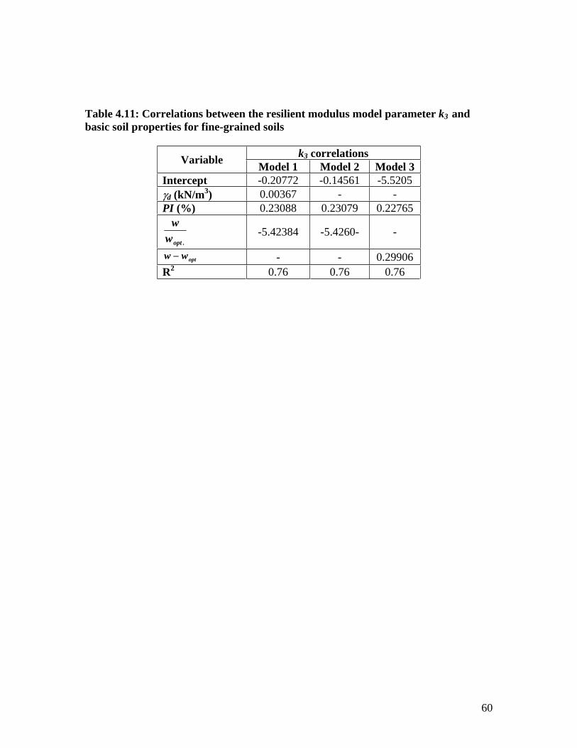
Table 4.11: Correlations between the resilient modulus model parameter k3 and
basic soil properties for fine-grained soils
Variable k3 correlations
Model 1 Model 2 Model 3
Intercept -0.20772 -0.14561 -5.5205
Jd (kN/m3) 0.00367 - -
PI (%) 0.23088 0.23079 0.22765
opt . w
w -5.42384 -5.4260- -
optww � - - 0.29906
R2 0.76 0.76 0.76
60

0
200
400
600
800
1000
1200
1400
1600
1800
k 1 e
stim
ated
fro
m b
asic
soil
pro
per
ties
Model-1
Model-2
Model-3
Model-4
0
200
400
600
800
1000
1200
1400
1600
1800
k1 estimated from repeated load triaxial test results
(a) k1
0 0.2 0.4 0.6 0.8 1
k2 estimated from repeated load triaxial test results
0
0.2
0.4
0.6
0.8
1
k 2 e
stim
ated
fro
m b
asic
soil
pro
per
ties
Model-1
Model-2
Model-3
(b) k2
Figure 4.16: Comparison of resilient modulus model parameters (ki) estimated from
soil properties and ki determined from results of repeated load triaxial test on
investigated fine-grained soils
61

k 3
est
imat
ed f
rom
bas
ic s
oil
pro
per
ties
-6 -5 -4 -3 -2 -1 0
k3 estimated from repeated load triaxial test results
Model-1
Model-2
Model-3
0
-1
-2
-3
-4
-5
-6
(c) k3
Figure 4.16 (cont.): Comparison of resilient modulus model parameters (ki)
estimated from soil properties and ki determined from results of repeated load
triaxial test on investigated fine-grained soils
62

Based on the statistical analysis on the results of the investigated fine-grained soils, the
resilient modulus model parameters (ki) can be estimated from basic soil properties using
the following equations:
§ · w k1 404.166 � 42.933PI � 52.260J d � 987.353 ̈ ¸ (4.8)¨ ¸w© opt ¹
§ w · § J · k2 0.25113 � 0.0292PI � 0.5573 ̈ ¸u¨ d ¸ (4.9)¨ ¸ ¨ ¸w© opt ¹ © J d max ¹
§ · w k3 �0.20772 � 0.23088PI � 0.00367J d � 5.4238 ̈ ¸ (4.10)¨ ¸w© opt ¹
where PI is the plasticity index, w is the moisture content of the soil, wopt. is the optimum
moisture content, Jd is the dry unit weight, and Jdmax is the maximum dry unit weight.
Table 4.12 presents the correlation matrix of soil properties used in the regression and
model parameters for fine-grained soils. A summary of regression coefficients obtained
for the fine-grained correlations with t-statistics at 95% confidence level is presented in
Tables 4.13. The overall significance of ki correlations was verified based on the F-test.
This means that ki and the estimated regression coefficients of independent variables for
all correlations constitute a linear relationship. The results of the t-statistics showed that,
(ignoring the significance of the intercept E0), the dry unit weight in both k1 and k3
models was insignificant in the case of fine-grained soils. The t-statistics were
determined as 1.23 and 0.01 for the k1 and k3 models, respectively. The t-statistics are not
significant if the absolute value of t0 (from table of parameter estimator) is less than tD/2,n
p-1 (from statistics tables). The minimum value of t0 for a parameter to be significant at
95% confidence level is 1.96 if a large population was considered. Although Jd in k1 and
k3 models for the fine-grained soils were found to be statistically insignificant, their
presence is physically sound based on engineering judgment.
Equations 4.8-4.10 were used in the resilient modulus constitutive Equation (4.1) to
estimate the resilient modulus of the investigated fine-grained soils. The results are
presented in Figure 4.17, which depicts the predicted versus the measured resilient
modulus values. Inspection of Figure 4.17 indicates that the resilient modulus of
compacted fine-grained soils can be estimated from Equation 4.1 and the correlations
proposed by Equations 4.8-4.10 with reasonable accuracy. It should be emphasized that
these correlations are developed based on analysis of test results on soils compacted at
high unit weight values (between 95 and 100% of Jdmax) with a moisture content range
around the optimum value.
63

Table 4.12: Correlation matrix of model parameters and soil properties for fine-
grained soils
Variable PI Jd w/wopt (w/wopt) u (Jd/Jdmax) k1 k2 k3
PI 1.00 -0.15 0.16 0.03 0.21 -0.32 0.08
Jd 1.00 -0.15 0.09 0.19 -0.15 0.06
w/wopt 1.00 0.95 -0.84 0.70 -0.85
(w/wopt)u(Jd/Jdmax) 1.00 -0.83 0.73 -0.86
k1 1.00 -0.89 0.79
k2 1.00 -0.82
k3 1.00
Table 4.13: Summary of t-statistics for regression coefficients used in resilient
modulus model parameters for fine-grained soils
Model k1 k2 k3
Parameter Parameter
estimator
t-statistic
(95% CL)
Parameter
estimator
t-statistic
(95% CL)
Parameter
estimator
t-statistic
(95% CL)
E0 404.166 0.55 0.25113 1.37 -0.2077 -0.04
E1 52.260 1.23 -0.02917 -2.49 0.0037 0.01
E2 42.933 3.55 0.55733 5.40 0.23088 2.55
E3 -987.353 -9.46 - - -5.4238 -6.66
R2 0.84 0.65 0.76
SEE 128.63 0.126 0.869
CL: confidence level, SEE: standard error of estimate
64

P
redi
cted
res
ilien
t mod
ulus
(M
Pa)
180
160
140
120
100
80
60
40
20
0
Fine-grained soils
0 20 40 60 80 100 120 140 160 180
Measured resilient modulus (MPa)
Figure 4.17: Predicted versus measured resilient modulus of compacted fine-grained
soils
65

Coarse-Grained Soils
Regression analysis conducted on the test results of the coarse-grained soils (less than
50% passing sieve #200) resulted in poor correlations between ki values and basic soil
properties. This is due to the fact that some of the investigated coarse-grained soils do not
have plasticity characteristics (non-plastic soils). Therefore, coarse-grained soils were
separated into two groups for the purpose of statistical analysis: plastic coarse-grained
soils and non-plastic coarse-grained soils. This treatment significantly improved the
proposed correlations between soil properties and ki. In addition, parameters related to the
grain size characteristics of coarse-grained soils such as coefficient of curvature (Cc),
coefficient of uniformity (Cu) and effective size (D10) were included in the analysis
(Table 4.14). These parameters did not improve the results of the statistical analysis and
therefore were excluded.
Table 4.14: Characteristics of particle size distribution curves of investigated
coarse-grained soils
Soil Type Cu Cc D10 (mm) D30(mm) D50(mm) D60(mm)
Beecher 102 1.29 9.04E-05 0.001 0.0038 0.0092
Goodman 82.91 1.15 0.0011 0.011 0.0422 0.0938
Plano 27.99 6.09 3.34E-04 0.0044 0.008 0.0094
Chetek 47.54 3.27 2.77E-04 0.0035 0.0106 0.0132
Eleva 29.6 6.2 8.00E-04 0.0109 0.0167 0.0232
Pence 38.35 3.93 5.12E-04 0.0063 0.014 0.0196
Gogebic 48.08 2.75 2.23E-04 0.0026 0.0079 0.0107
Ontonagon-C-1 32.19 4.1 2.39E-04 0.0027 0.0069 0.0077
Ontonagon-C-2 23.74 6.53 3.69E-04 0.0046 0.0076 0.0088
Kewaunee-1 28.8 4.58 2.57E-04 0.003 0.0061 0.0074
Kewaunee-2 110.2 1.2 8.88E-05 0.001 0.0038 0.0098
Plainfield 2.38 0.92 0.0066 0.0098 0.0132 0.0158
Sayner-Rubicon 3.03 0.83 0.0093 0.0143 0.0228 0.0281
Shiocton 30.54 4.32 1.25E-04 0.0014 0.0033 0.0038
Withee 47.6 2.77 1.82E-04 0.0021 0.0061 0.0087
Cc = coefficient of curvature, Cu = coefficient of uniformity, D10 = effective size,
D30 = particle size corresponding to 30% finer, D50 = median size, D60 = particle size
corresponding to 60% finer.
A summary of the regression analysis on non-plastic coarse-grained soils is presented in
Tables 4.15-4.17. The resilient modulus model parameters ki can be estimated from basic
soil properties using the models presented in Tables 4.15-4.17. Figure 4.18 depicts
comparisons between ki values obtained from analysis of the results of the repeated load
triaxial test and ki values estimated from basic soil properties using the correlations
presented in Tables 4.15-4.17. An examination of Figure 4.18 shows that ki prediction
models are acceptable with R2 values range from 0.59 to 0.79. These correlations were
66
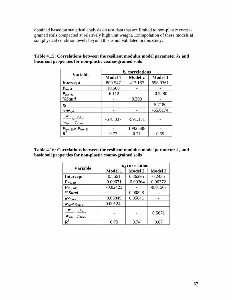
obtained based on statistical analysis on test data that are limited to non-plastic coarse-
grained soils compacted at relatively high unit weight. Extrapolation of these models at
soil physical condition levels beyond this is not validated in this study.
Table 4.15: Correlations between the resilient modulus model parameter k1 and
basic soil properties for non-plastic coarse-grained soils
Variable k1 correlations
Model 1 Model 2 Model 3
Intercept 809.547 417.187 698.0361
PNo. 4 10.568 - -
PNo. 40 -6.112 - -0.2280
%Sand - 8.203 -
Jd - - 5.7180
w-wopt - - -55.0174
max. d
d
optw
w
J J
u -578.337 -591.151 -
PNo. 200/ PNo. 40 - 1092.588 -
R2 0.72 0.71 0.69
Table 4.16: Correlations between the resilient modulus model parameter k2 and
basic soil properties for non-plastic coarse-grained soils
Variable k2 correlations
Model 1 Model 2 Model 3
Intercept 0.5661 0.36295 0.2435
PNo. 40 0.00671 -0.00364 0.00372
PNo. 200 -0.02423 - -0.01567
%Sand - 0.00828 -
w-wopt 0.05849 0.05641 -
woptuJdmax 0.001242 - -
max. d
d
optw
w
J J
u - - 0.5671
R2 0.79 0.74 0.67
67

Table 4.17: Correlations between the resilient modulus model parameter k3 and
basic soil properties for non-plastic coarse-grained soils
Variable k3 correlations
Model 1 Model 2 Model 3
Intercept -0.50792 2.4747 -1.7529
PNo. 4 - - 0.8472
PNo. 40 -0.041411 0.02541 0.0403
PNo. 200 0.14820 - -0.8765
%Sand - -0.06859 -0.8849
w-wopt -0.1726 -0.17352 -0.17176
woptuJdmax -0.01214 -0.00873 -
R2 0.67 0.65 0.59
68

0
200
400
600
800
1000
1200
1400
k 1 e
stim
ated
fro
m b
asic
soil
pro
per
ties
Model-1
Model-2
Model-3
0
200
400
600
800
1000
1200
1400
k1 estimated from repeated load triaxial test results
(a) k1
0
0.2
0.4
0.6
0.8
1
1.2
k 2 e
stim
ated
fro
m b
asic
soil p
rop
erties
Model-1
Model-2
Model-3
0 0.2 0.4 0.6 0.8 1 1.2
k2 estimated from repeated load triaxial test results
(b) k2
Figure 4.18: Comparison of resilient modulus model parameters (ki) estimated from
soil properties and ki determined from results of repeated load triaxial test on
investigated non-plastic coarse-grained soils
69

k 3 e
stim
ated
fro
m b
asic
soil
pro
per
ties
0
-1
-2
-3
-4
-5
Model-1
Model-2
Model-3
-5 -4 -3 -2 -1 0
k3 estimated from repeated load triaxial test results
(c) k3
Figure 4.18 (cont.): Comparison of resilient modulus model parameters (ki)
estimated from soil properties and ki determined from results of repeated load
triaxial test on investigated non-plastic coarse-grained soils
70

Based on statistical analysis on the investigated non-plastic coarse-grained soils, the
resilient modulus model parameters (ki) can be estimated from basic soil properties using
the following equations:
§ w · § J · k1 809.547 �10.568PNo.4 � 6.112PNo.40 � 578.337 ̈ ¸u ¨̈ ¸̧ (4.11)¨ ¸
d
w J© opt ¹ © d max ¹
k 0.5661� 0.006711P � 0.02423P � 0.05849(w � w )2 No.40 No.200 opt (4.12)
� 0.001242(w ) u (J )opt d max
k �0.5079 � 0.041411P � 0.14820P � 0.1726(w � w )3 No.40 No.200 opt (4.13)
� 0.01214(w )u (J )opt d max
where PNo.4 is percent passing sieve #4, PNo.40 is percent passing sieve #40, PNo.200 is
percent passing sieve #200, w is the moisture content of the soil, wopt. is the optimum
moisture content, Jd is the dry unit weight, and Jdmax is the maximum dry unit weight.
The correlation matrix for basic soil properties and ki of non-plastic coarse-grained soils
is presented in Table 4.18. A summary of regression coefficients obtained for non-plastic
coarse-grained soils correlations with t-statistics at 95% confidence level is presented in
Table 4.19. For non-plastic coarse-grained soils, ki models were significant based on the
F-test. With the exception of the intercept in k3 model, all independent variables used in ki
models were significant based on t0 (from table of parameters estimates). The absolute
value of t0 for the intercept in k3 is 1.
Equations 4.11-4.13 were used to estimate the resilient modulus of the investigated non-
plastic coarse-grained soils. Figure 4.19 depicts comparison of the predicted versus
measured resilient modulus values using these equations. Examination of Figure 4.19
demonstrates that the estimated resilient modulus values of compacted non-plastic
coarse-grained soils are consistent with values obtained from repeated load triaxial test
results. It should be emphasized that these correlations are developed on analysis of test
results on soils compacted at high unit weight values (between 95 and 100% of Jdmax)
with moisture content range around the optimum value.
71

Table 4.18: Correlation matrix of model parameters and soil properties for non-
plastic coarse-grained soils
Variable PNo.4 PNo.40 PNo.200 w-wopt woptuJdmax d max
d
optw
w
J J
u k1 k2 k3
PNo.4 1.00 0.88 0.68 0.03 -0.04 0.03 0.05 -0.05 0.07
PNo.40 1.00 0.84 0.09 -0.00 0.09 -0.10 -0.10 0.19
PNo.200 1.00 0.11 0.32 0.12 -0.1 -0.19 0.29
w-wopt 1.00 -0.14 0.96 -0.83 0.81 -0.51
woptuJdmax 1.00 -0.11 0.02 -0.11 -0.18
d max
d
optw
w
J J
u 1.00 -0.82 0.75 -0.45
k1 1.00 -0.84 0.55
k2 1.00 -0.81
k3 1.00
Table 4.19: Summary of t-statistics for regression coefficients used in resilient
modulus model parameters for non-plastic coarse-grained soils
Model
Parameter
k1 k2 k3
Parameter
estimator
t-statistic
(95% CL)
Parameter
estimator
t-statistic
(95% CL)
Parameter
estimator
t-statistic
(95% CL)
E0 809.547 3.48 0.5661 5.38 -0.5079 -1.00
E1 10.568 2.75 -0.02423 -4.76 0.1482 6.03
E2 -6.112 -2.61 0.00671 3.22 -0.041411 -4.12
E3 -578.337 -9.65 0.05849 11.98 -0.1726 -7.33
E4 - - 0.001242 2.95 -0.01214 -5.98
R2 0.72 0.79 0.67
SEE 119.9 0.104 0.503
CL: confidence level, SEE: standard error of estimate
72

180
Non-plastic coarse-grained soils 160
140
120
100
80
60
40
20
0 0 20 40 60 80 100 120 140 160 180
Measured resilient modulus (MPa)
Figure 4.19: Predicted versus measured resilient modulus of compacted non-plastic
coarse-grained soils
Pre
dict
ed r
esili
ent m
odul
us (
MP
a)
73

The results of the regression analysis on plastic coarse-grained soils are summarized in
Tables 4.20-4.22. The results are also presented in Figure 4.20 which depicts
comparisons between ki values obtained from analysis of repeated load triaxial test results
and ki values estimated from basic soil properties. Inspection of Figure 4.20 shows that
the predicted ki are consistent with values obtained from test results. The coefficient of
multiple determination for the correlations varies between 0.58 and 0.83. These
correlations were obtained based on statistical analysis on test data that are limited to
plastic coarse-grained soils compacted at relatively high unit weight. Extrapolation of
these models at soil physical condition levels beyond this was not validated in this study.
Table 4.20: Correlations between the resilient modulus model parameter k1 and
basic soil properties for plastic coarse-grained soils
Variable k1 correlations
Model 1 Model 2 Model 3
Intercept 3596.445 5156.468 8642.873
PNo. 200 -55.975 -63.829 132.643
%Silt - - -428.067
LL -85.870 -87.526 -
PI - - -254.685
Jd - 75.395 197.230
Jd / Jdmax 2948.246 - -
w/wopt -360.099 - -381.400
(w-wopt)/wopt - -345.612 -
R2 0.83 0.76 0.83
Table 4.21: Correlations between the resilient modulus model parameter k2 and
basic soil properties for plastic coarse-grained soils
Variable k2 correlations
Model 1
Intercept 2.3250
PNo. 200 -0.00853
LL 0.02579
PI -0.06224
Jd / Jdmax -1.73380
w/wopt 0.20911
R2 0.58
74

Table 4.22: Correlations between the resilient modulus model parameter k3 and
basic soil properties for plastic coarse-grained soils
Variable k3 correlations
Model 1 Model 2 Model 3
Intercept -25.9374 -21.3497 -32.5449
PNo. 200 0.7680 - 0.7691
%Silt -1.1371 - -1.1370
LL - -0.2961 -
PI - 0.3618 -
Jd / Jdmax 31.4444 29.9702 31.5542
w/wopt -6.4483 -6.0909 -
w-wopt - - -0.4128
R2 0.80 0.81 0.82
75

0
200
400
600
800
1000
1200
1400
k 1 e
stim
ated
fro
m b
asic
soil
pro
per
ties
Model-1
Model-2
Model-3
0
200
400
600
800
1000
1200
1400
k1 estimated from repeated load triaxial test results
(a) k1
k 2 e
stim
ated
fro
m b
asic
so
il p
rop
erties
0.2
0.4
0.6
0.8
Model-1
0
0 0.2 0.4 0.6 0.8
k2 estimated from repeated load triaxial test results
(b) k2
Figure 4.20: Comparison of resilient modulus model parameters (ki) estimated from
soil properties and ki determined from results of repeated load triaxial test on
investigated plastic coarse-grained soils
76

k 3
est
imat
ed f
rom
bas
ic s
oil
pro
per
ties
-7 -6 -5 -4 -3 -2 -1 0
k3 estimated from repeated load triaxial test results
Model-1
Model-2
Model-3
0
-1
-2
-3
-4
-5
-6
-7
(c) k3
Figure 4.20 (cont.): Comparison of resilient modulus model parameters (ki)
estimated from soil properties and ki determined from results of repeated load
triaxial test on investigated plastic coarse-grained soils
77
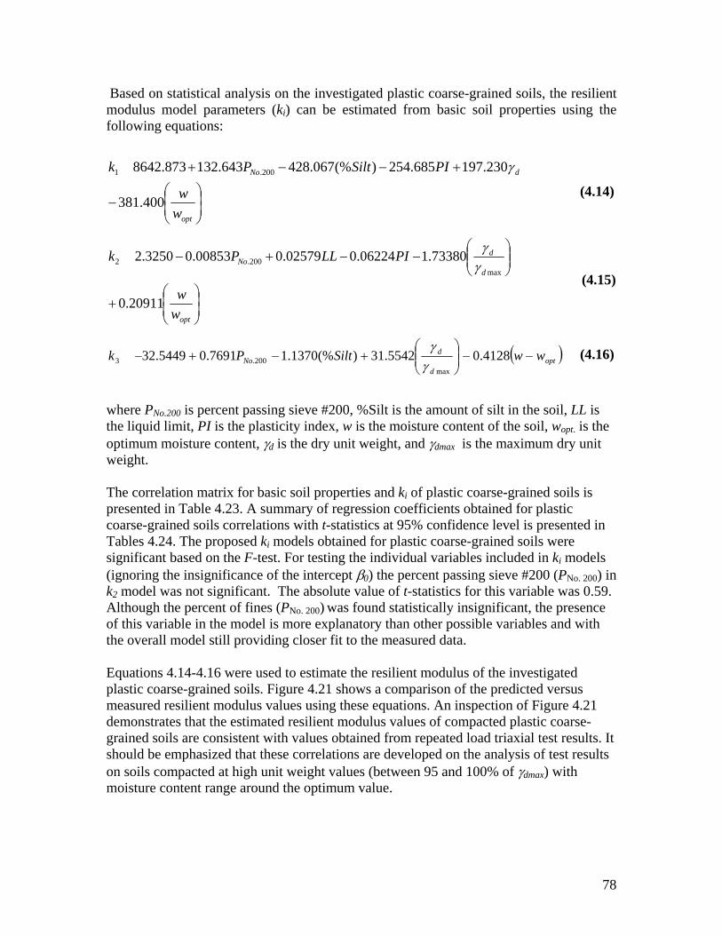
Based on statistical analysis on the investigated plastic coarse-grained soils, the resilient
modulus model parameters (ki) can be estimated from basic soil properties using the
following equations:
k 8642.873 �132.643P � 428.067(%Silt) � 254.685PI �197.230J1 No.200 d
§ w · (4.14)� 381.400 ̈ ¸
¨ ¸w© opt ¹
§ J d ·
k 2.3250 � 0.00853P � 0.02579LL � 0.06224PI �1.73380¨ ¸2 No.200 ¨ ¸J© d max ¹
(4.15)§ · w¨ ¸� 0.20911¨ ¸w© opt ¹
§ J d ·
k3 �32.5449 � 0.7691PNo.200 � 1.1370(%Silt) � 31.5542¨̈ ¸̧ � 0.4128�w � wopt � (4.16)J© d max ¹
where PNo.200 is percent passing sieve #200, %Silt is the amount of silt in the soil, LL is
the liquid limit, PI is the plasticity index, w is the moisture content of the soil, wopt. is the
optimum moisture content, Jd is the dry unit weight, and Jdmax is the maximum dry unit
weight.
The correlation matrix for basic soil properties and ki of plastic coarse-grained soils is
presented in Table 4.23. A summary of regression coefficients obtained for plastic
coarse-grained soils correlations with t-statistics at 95% confidence level is presented in
Tables 4.24. The proposed ki models obtained for plastic coarse-grained soils were
significant based on the F-test. For testing the individual variables included in ki models
(ignoring the insignificance of the intercept E0) the percent passing sieve #200 (PNo. 200) in
k2 model was not significant. The absolute value of t-statistics for this variable was 0.59.
Although the percent of fines (PNo. 200) was found statistically insignificant, the presence
of this variable in the model is more explanatory than other possible variables and with
the overall model still providing closer fit to the measured data.
Equations 4.14-4.16 were used to estimate the resilient modulus of the investigated
plastic coarse-grained soils. Figure 4.21 shows a comparison of the predicted versus
measured resilient modulus values using these equations. An inspection of Figure 4.21
demonstrates that the estimated resilient modulus values of compacted plastic coarse-
grained soils are consistent with values obtained from repeated load triaxial test results. It
should be emphasized that these correlations are developed on the analysis of test results
on soils compacted at high unit weight values (between 95 and 100% of Jdmax) with
moisture content range around the optimum value.
78

Table 4.23: Correlation matrix of model parameters and soil properties for plastic
coarse-grained soils
Variable PNo.200 %Silt LL PI Jd d max
d
J J
w/wopt w
wopt k1 k2 k3
PNo.200 1.00 0.99 -0.96 -0.99 0.79 0.01 0.06 0.07 0.34 0.37 0.11
%Silt 1.00 0.96 -0.99 0.78 -0.00 0.06 0.06 0.31 0.40 0.09
LL 1.00 0.97 -0.79 -0.05 -0.02 -0.03 -0.52 -0.27 -0.22
PI 1.00 -0.75 -0.01 -0.04 -0.04 -0.38 -0.39 -0.13
Jd 1.00 0.50 0.07 0.07 0.46 0.06 0.29
d max
d
J J
1.00 0.05 0.05 0.41 0.39 0.44
w/wopt 1.00 0.99 -0.37 0.35 -0.70
w-wopt 1.00 -0.36 0.33 -0.71
k1 1.00 -0.48 0.81
k2 1.00 -0.61
k3 1.00
Table 4.24: Summary of t-statistics for regression coefficients used in resilient
modulus model parameters for plastic coarse-grained soils
Model
Parameter
k1 k2 k3
Parameter
estimator
t-statistic
(95% CL)
Parameter
estimator
t-statistic
(95% CL)
Parameter
estimator
t-statistic
(95% CL)
E0 8642.873 5.66 2.32504 1.77 -32.5449 -4.93
E1 197.230 4.92 -0.00853 -0.59 0.7691 2.76
E2 132.634 3.55 0.02579 2.23 -1.1370 -2.65
E3 -254.685 -6.48 -0.06224 -2.25 31.5542 4.74
E4 -428.067 -6.19 -1.73380 -2.36 -0.4128 -8.08
E5 -381.400 -3.48 0.20911 2.30 - -
R2 0.83 0.58 0.82
SEE 112.71 0.093 0.849
CL: confidence level, SEE: standard error of estimate
79
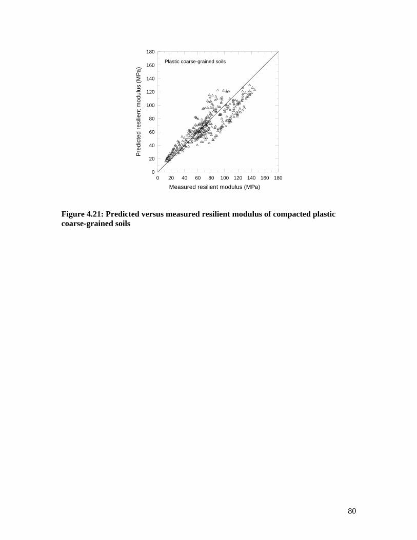
0 20 40 60 80 100 120 140 160 180 0
20
40
60
80
100
120
140
160
180
Pre
dict
ed r
esili
ent m
odul
us (
MP
a)
Plastic coarse-grained soils
Measured resilient modulus (MPa)
Figure 4.21: Predicted versus measured resilient modulus of compacted plastic
coarse-grained soils
80

4.4 Predictions Using LTPP Models
In order to inspect the performance of the models developed in this study, comparison
with the models developed by Yau and Von Quintus (2004) based on the Long Term
Pavement Performance database was made. It should be noted that the data used to
develop LTPP models and the database of this study are not similar. One difference is
that the AASHTO T 307 was used herein to perform the repeated load triaxial test. Other
sources that may affect the outcome include sample preparation and nature of soils
samples (undisturbed versus compacted).
LTPP models (Yau and Von Quintus, 2004) are used to predict the resilient modulus of
Wisconsin subgrade soils from the test results of this study. The resilient modulus values
of Wisconsin subgrade soils predicted by LTPP models are then compared to the values
obtained from test results and to the values predicted by the models developed herein.
The LTPP prediction models (Yau and Von Quintus, 2004) used are presented in the
following equations:
LTPP equations for clay soils
k1 1.3577 � 0.0106�%Clay�� 0.0437w (4.17)
k 0.5193 � 0.0073PNo.4 � 0.0095PNo.40 � 0.0027PNo � 0.0030LL2 .200 (4.18)
� 0.0049wopt
k 1.4258 � 0.0288P � 0.0303P � 0.0521P � 0.0251(%Silt)3 No.4 No.40 No.200
§ w · (4.19)� 0.0535LL � 0.0672wopt � 0.0026J d max � 0.0025J d � 0.6055 ̈ ¸
¨ ¸w© opt ¹
LTPP equations for silt soils
k1 1.0480 � 0.0177(%Clay) � 0.0279PI � 0.0370w (4.20)
k2 0.5097 � 0.0286PI (4.21)
k3 �0.2218 � 0.0047(%Silt) � 0.0849PI � 0.1399w (4.22)
81
LTPP equations for sand soils
k1 3.2868 � 0.0412P � 0.0267PNo.4 � 0.0137(%Clay) � 0.0083LL � 0.0379wopt3 / 8 (4.23)
� 0.0004J d
k 0.5670 � 0.0045P � 2.98u10�5 P � 0.0043(%Silt) � 0.0102(%Clay)2 3 / 8 No.4
§ J · § · (4.24)w5� 0.0041LL � 0.0014wopt � 3.41u10� J d � 0.4582¨ d ¸ � 0.1779 ̈ ¸¨ ¸ ¨ ¸J w© d max ¹ © opt ¹
k3 �3.5677 � 0.1142P3/8 � 0.0839PNo.4 � 0.1249P200 � 0.1030(%Silt) � 0.1191(%Clay)
(4.25)§ J d · § w ·
� 0.0069LL � 0.0103wopt � 0.0017J d � 4.3177¨ ¸ �1.1095 ̈ ¸¨ ¸ ¨ ¸J w© d max ¹ © opt ¹
LTPP equations for all soils:
k 0.9848 � 0.0050P � 0.0011P � 0.0085(%Clay) � 0.0089LL1 3/8 No.40
§ · (4.26)w� 0.0094PI � 0.0235w � 0.3290 ̈ ¸
¨ ¸w© opt ¹
k2 0.4808 � 0.0037P3/8 � 0.0062PNo.4 � 0.0016PNo.40 � 0.0008PNo.200 � 0.0018(%Clay)
(4.27)§ J d · § w ·
� 0.0078LL � 0.0019PI � 0.0111w � 0.1232¨ ¸ � 0.0009 ̈ ¸¨ ¸ ¨ ¸J w© d max ¹ © opt ¹
k 9.6691� 0.0302P � 0.0065P � 0.0192P � 0.0115P � 0.0040(%Clay)3 3/8 No.4 No.40 200
§ J d · (4.28)
� 0.0075LL � 0.0401PI � 0.0020wopt � 0.0039J d max � 0.2750w � 0.7177¨ ¸ ¨ ¸J© d max ¹ 2§ w · § �J max � ·
�1.0262 ̈ ¸ � 5.28x10�6 ¨ d ¸¨ ¸ ¨ ¸© wopt ¹ © PNo.40 ¹
Figures 4.22-4.24 present comparisons of predicted and measured resilient modulus of
fine-grained, non-plastic coarse-grained, and plastic coarse-grained Wisconsin soils using
the LTPP models (Yau and Von Quintus, 2004). Inspection of Figures 4.22- 4.24
demonstrates that the models developed herein were able to estimate the resilient
modulus of Wisconsin compacted soils better than the models of the LTPP study. The
difference in the test procedures and other conditions involved with development of both
LTPP and the models of this study contributed to this outcome.
82

20
40
60
80
100
120
140
160
180 180
Fine grained soils Fine grained soils 160 LTPP model for silt soils
140
Pre
dic
ted
res
ilie
nt
mo
du
lus
(MP
a)
Pre
dic
ted r
esil
ient
modulu
s (M
Pa)
Pre
dic
ted
res
ilie
nt
modu
lus
(MP
a)
120
100
80
60
40
20
0 0
0 20 40 60 80 100 120 140 160 180 0 20 40 60 80 100 120 140 160 180
Measured resilient modulus (MPa) Measured resilient modulus (MPa)
(a) Using proposed model (b) Using LTPP silt model
180
160 Fine grained soils
LTPP model for all soils
140
120
100
80
60
40
20
0
0 20 40 60 80 100 120 140 160 180
Measured resilient modulus (MPa)
(c) Using LTPP model for combined (all) subgrade soils
Figure 22: Predicted versus measured resilient modulus of Wisconsin fine-grained
soils using the mode developed in this study and the LTPP database developed
models
83

20
40
60
80
100
120
140
180 180
160 Non plastic coarse grained soils 160 Proposed model
140
Pre
dic
ted
res
ilie
nt
modu
lus
(MP
a)P
redic
ted
res
ilie
nt
modu
lus
(MP
a)
Pre
dic
ted
res
ilie
nt
modu
lus
(MP
a)
120
100
80
60
40
Non plastic coarse grained soils 20
LTPP sand model
0 0
0 20 40 60 80 100 120 140 160 180 0 20 40 60 80 100 120 140 160 180
Measured resilient modulus (MPa) Measured resilient modulus (MPa)
(a) Using proposed model (b) Using LTPP sand model
180
160 Non plastic coarse grained soils
LTPP model for all soils
140
120
100
80
60
40
20
0
0 20 40 60 80 100 120 140 160 180
Measured resilient modulus (MPa)
(c) Using LTPP model for combined (all) subgrade soils
Figure 23: Predicted versus measured resilient modulus of Wisconsin non-plastic
coarse-grained soils using the mode developed in this study and the LTPP database
developed models
84

20
40
60
80
100
120
140
160
180 180
Plastic coarse grained soils 160Plastic coarse grained soils LTPP sand model
Proposed model 140
Pre
dic
ted
res
ilie
nt
mod
ulu
s (M
Pa)
Pre
dic
ted
res
ilie
nt
modu
lus
(MP
a)
Pre
dic
ted
res
ilie
nt
modu
lus
(MP
a)
120
100
80
60
40
20
0 0
0 20 40 60 80 100 120 140 160 180 0 20 40 60 80 100 120 140 160 180
Measured resilient modulus (MPa) Measured resilient modulus (MPa)
(a) Using proposed model (b) Using LTPP sand model
180
160 Plastic coarse grained soils
LTPP model for all soils
140
120
100
80
60
40
20
0
0 20 40 60 80 100 120 140 160 180
Measured resilient modulus (MPa)
(c) Using LTPP model for combined (all) subgrade soils
Figure 24: Predicted versus measured resilient modulus of Wisconsin plastic coarse-
grained soils using the mode developed in this study and the LTPP database
developed models
85

Chapter 5
Conclusions and Recommendations
This research report presented the results of a comprehensive study conducted to evaluate
the resilient modulus of common Wisconsin subgrade soils. The primary objective of this
research project was to develop a methodology for estimating the resilient modulus of
various Wisconsin subgrade soils from basic soil properties. This was achieved by
carrying out laboratory-testing program on common Wisconsin subgrade soils. The
program included tests to evaluate basic soil properties and repeated load triaxial tests to
determine the resilient modulus. High quality test results were obtained in this study by
insuring the repeatability of results and also by performing two tests on each soil replicate
specimens at the specified physical condition.
The resilient modulus model given by Equation 4.1 is the constitutive equation developed
by NCHRP project 1-28A and adopted by the NCHRP project 1-37A for the “Guide for
Mechanistic-Empirical Design of New and Rehabilitated Pavement Structures.” This
study focused on developing correlations between basic soil properties and the
parameters k1, k2, and k3 (Equation 4.1).
The laboratory-testing program provided the research team with high quality database
that was utilized to develop and validate correlations between resilient modulus model
parameters and basic soil properties. Comprehensive statistical analysis including
multiple linear and nonlinear regression was performed to develop these correlations.
Statistical analysis conducted on all test results combined did not produce good
correlations between model parameters and basic soil properties. When test results for
coarse-grained and fine-grained soils were treated separately, good correlations were
obtained. Comparisons of predicted and measured resilient modulus values indicated that
the correlations proposed by this study are of acceptable accuracy.
The LTPP resilient modulus models (Yau and Von Quintus, 2004) were used to predict
the resilient modulus of Wisconsin subgrade soils from the test results of this study.
Comparisons of predicted and measured resilient modulus showed that the LTPP models
did not yield good results compared to the models proposed herein.
Based on the results of this research, the following conclusions are reached:
1. The repeated load triaxial test (which is specified by AASHTO to determine the
resilient modulus of subgrade soils for pavement design) is complicated, time
consuming, expensive, and requires advanced machine and skilled operators.
2. The results of the repeated load triaxial test on the investigated Wisconsin
subgrade soils provide resilient modulus database that can be utilized to estimate
values for mechanistic-empirical pavement design in the absence of basic soils
testing (level 3 input parameters)
86

3. The equations that correlate resilient modulus model parameters (k1, k2, and k3) to
basic soil properties for fine-grained and coarse-grained soils can be utilized to
estimate level 2 resilient modulus input for the mechanistic-empirical pavement
design. These equations are presented in Chapter 4.
4. The equations (models) developed in this research were based on statistical
analysis of laboratory test results that were limited to the soil physical conditions
specified. Estimation of resilient modulus of subgrade soils beyond these
conditions was not validated.
Based on the results of this research, the research team recommends the following:
1. The use of the resilient modulus test database in the absence of any basic soil
testing when designing low volume roads as indicated by AASHTO.
2. The use of the equations provided in Chapter 4 to estimate the resilient modulus
of subgrade soils from basic soil properties. There are on average three different
models to estimate each ki for each soil type (fine-grained, non-plastic coarse-
grained, and plastic coarse-grained). These equations can be used based on
available basic soil test results.
3. Further research is needed to explore newly developed field devices such as light
drop weight. This can provide Wisconsin DOT and contractors with field tools to
assure quality of compacted subgrade soils in terms of stiffness.
4. Further research is needed to explore the effect of freeze-thaw cycles on the
resilient modulus of Wisconsin subgrade soils. This is essential since the resilient
modulus is highly influenced by the seasonal variations in moisture and extreme
temperatures.
87

References
AASHTO 2002 Guide for Mechanistic-Empirical Design of New and Rehabilitated
Pavement Structures. NCHRP Project 1-37A Final Report by ERES Consultants, March
2004.
Allen, A. J. (1996). Development of A Correlation Between Physical and Fundamental
Properties of Louisiana Soils. Master’s Thesis, Dept. of Civil Eng., Louisiana State
University, Baton Rouge.
Barksdale, R. D. (1972). “A Laboratory Evaluation of Rutting in Base Course Materials,”
Proceedings of the 3rd
International Conference on the Structural Design of Asphalt Pavements, University of Michigan, pp. 161-174.
Barksdale, R. D., Rix, G.J., Itani, S., Khosla, P.N., Kim, R., Lambe, C., and Rahman,
M.S., (1990). “Laboratory Determination of Resilient Modulus for Flexible Pavement
Design,” NCHRP, Transportation Research Board, Interim Report No. 1-28, Georgia
Institute of Technology, Georgia.
Butalia, T. S., Huang, J., Kim, D. G., and Croft, F., (2003). “Effect of Moisture Content
and Pore Water Pressure Build on Resilient Modulus of Cohesive Soils,” Resilient
Modulus Testing for Pavement Components, ASTM STP 1437.
Chamberlain, E.J., Cole, D. M., and Durell, G. F., (1989). “Resilient Modulus
Determination for Frost Conditions, State of the Art Pavement Response Monitoring
Systems for Roads and Air Field,” Special Report 89-23, U.S. Army Cold Region
Research and Engineering Laboratory (CRREL), Hanover, H, 1989, pp. 230-333.
Chou, Y. T., (1976) “Evaluation of Nonlinear Resilient Modulus of Unbound Granular
Materials from Accelerated Traffic Test Data,” U.S. Army Engineer Waterways
Experiment Station, Vicksburg, MS, Final Technical Report.
Drumm, E. C., Boateng-Poku, Y., and Pierce, T. J. (1990). “Estimation of Subgrade
Resilient Modulus from Standard Tests,” Journal of Geotechnical Engineering, Vol. 116,
No. 5, pp. 774-789.
Drumm E. C., Reeves, J. S., Madgett, M. R., and Trolinger, W. D. (1997). “Subgrade
Resilient Modulus Correction for Saturation Effects,” Journal of Geotechnical and
Geoenvironmental Engineering, Vol. 123, No. 7.
Fredlund, D.G., Bergan, A. T. and Wong, P. K. (1977). “Relation Between Resilient
Modulus and Stress Research Conditions for Cohesive Subgrade Soils” Transportation
Research Record No. 642, Transportation Research Board, pp.73-81.
Groeger, J. L., Rada, G. R., and Lopez, A. (2003). “AASHTO T 307-Background and
Discussion,” Resilient Modulus Testing for Pavement Components, ASTM STP 1437.
88

Heydinger, A. G., (2003). “Evaluation of Seasonal Effects on Subgrade Soils,”
Transportation Research Record No. 1821, Transportation Research Board, pp.47-55.
Hines, William W. and Montgomery, Douglas C (1980). Probability and Statistics in
Engineering and Management Science. 2nd Edition, John Willey & Sons Inc., New York.
Hole, F. D. (1980) “Soil Guide For Wisconsin Land Lookers.” Bul. 88, Soil Series No.
63, Geological and Natural History Survey University of Wisconsin-Extension and
University of Wisconsin-Madison.
Hole, F. D. (1974). “Soil Regions of Wisconsin,” Geological and Natural History Survey
University of Wisconsin-Extension, (Map).
Huang, J. 2001. Degradation of Resilient Modulus of Saturated Clay Due to Pore Water
Pressure Buildup under Cyclic Loading, Master Thesis, Department of Civil Engineering
and Environmental Engineering, The Ohio State University.
Janoo, V.C., and Bayer II J.J. (2001). “The effect of Aggregate Angularity on Base
Course Performance,” U.S. Army Corps of Engineers, ERDC/CRREL TR-01-14.
Lekarp, F., Isacsson, U. and Dawson, A. (2000). “State of the Art. I: Resilient Response
of Unbound Aggregates,” Journal of Transportation Engineering, Vol. 126, No. 1.
Li, D., and Selig, E. T. (1994). “Resilient Modulus for Fine Grained Subgrade Soils,”
Journal of Geotechnical Engineering, Vol. 120, No. 6.
Maher, A., Bennert T., Gucunski, N., and Papp, W. J., (2000) “Resilient Modulus of New
Jersey Subgrade Soils,” FHWA Report No. 2000-01, Washington D.C.
May, R. W., and Witczak, M. W. (1981). “Effective Granular Modulus to Model
Pavement Responses,” Transportation Research Record No. 810, Transportation
Research Board, pp. 1-9.
Madison, F. W., and Gundlach, H. F. (1993). “Soil Regions of Wisconsin,” Wisconsin
Geological and Natural History Survey and U.S. Department of Agriculture, (Map).
Nazarian, S., and Feliberti, M. (1993). “Methodology for Resilient Modulus Testing of
Cohesionless Subgrades,” Transportation Research Record No. 1406, Transportation
Research Board, pp.108-115.
NCHRP Project 1-37A Summary of the 2000, 2001, and 2002 AASHTO Guide for The
Design of New and Rehabilitated Pavement Structures, NCHRP, Washington D.C.
Ooi, Philip S. K., Archilla A. R, and Sandefur K. G. (2004). “Resilient Modulus Models
for Compacted Cohesive Soils,” Transportation Research Record No. 1874,
89

Transportation Research Board, National Research Council, Washington, D. C., 2004, pp.
115-124.
Pezo, R. and Hudson, W. R. (1994). “Prediction Models of Resilient Modulus for
Nongranular Materials,” Geotechnical Testing Journal, GTJODJ, Vol. 17 No. 3, pp. 349
355.
Pezo, R., Claros, G., Hudson, W.R., and Stoke, K.H., (1992). “Development of a Reliable
Resilient Modulus Test for Subgrade and Non-Granular Subbase Materials For Use in A
Routine Pavement Design,” Research Report 1177-4F., University of Texas-Austin.
Rada, G., and Witczak, M. W. (1981). “Comprehensive Evaluation of Laboratory
Resilient Moduli Results for Granular Material,” Transportation Research Record No.
810, Transportation Research Board, pp. 23-33.
Scrivner, F.H., R., Peohl, W.M. Moore and M.B. Phillips (1969). “Detecting Seasonal
Changes in Load-Carrying Capabilities of Flexible Pavements,” NCHRP Report 7,
Highway Research Board, National Research Council, Washington, D.C.
Seed, H., Chan, C., and Lee, C. (1962). “Resilient Modulus of Subgrade Soils and Their
Relation to Fatigue Failures in Asphalt Pavements,” Proceedings, International
Conference on the Structural Design of Asphalt Pavements, University of Michigan, Ann
Arbor, Michigan, 611-636.
Smith, W. S., and Nair, K. (1973). “Development of Procedure for Characterization of
Untreated Granular Base Course and Asphalt Treated Course Materials,” FHWA, Final
Report, FHWA-A-RD-74-61, Washington D.C.
Thompson, M. R. and Q.L. Robnett (1979). “Resilient Properties of Subgrade Soils”
Transportation Engineering Journal, ASCE, 105(TE1), pp. 71-89.
Thomson, M. R., and Robnett, Q. L., (1976). “Resilient Properties of Subgrade Soils,”
Final Report, Illinois Cooperative Highway and Transportation Serial No. 160,
University of Illinois Urbana Champaign.
Titi, H. H., Elias, M. B., and Helwany, S. (2005). “Effect of Sample Size on Resilient
Modulus of Cohesive Soils,” Proceedings of the 16th
International Conference on Soil
Mechanics and Geotechnical Engineering (ICSMG), Osaka, Japan, September 12-16,
2005, Vol. 2, pp. 499-502.
Titi, H. H., Mohammad, L. N., and Herath, A. (2003). “Characterization of Resilient
Modulus of Coarse-Grained Materials Using the Intrusion Technology,” Special
Technical Publication 1437: Resilient Modulus Testing for Pavement Components,
American Society for Testing and Materials pp. 252-270.
90

Uzan, J. (1985) “Characterization of Granular Material,” Transportation Research
Record No. 1022, pp. 52-59.
Yau, A., and Von Quintus (2004). “Predicting Elastic Response Characteristics of
Unbound Materials and Soils,” Transportation Research Record No. 1874,
Transportation Research Board, National Research Council, Washington, D. C., pp. 47
56.
Zaman, M., Chen, D., and Larguros, J. (1994). “Resilient Modulus of Granular
Materials,” Journal of Transportation Engineering. Vol. 120, No. 6, pp. 967-988.
91

Appendix A

Per
cent
fine
r (%
)
Particle size (inch)
1 0.1 0.01 0.001 0.0001
100
80
60
40
20
0
Antigo soil
100 10 1 0.1 0.01 0.001 Particle size (mm)
Figure A.1: Particle size distribution curve for Antigo soil
16
17
18
19
Dry
uni
t wei
gh
t, J d
(kN
/m3 )
102
104
106
108
110
112
114
116
118
120
Dry
uni
t wei
ght, J d
(pcf
)
Antigo soil Test 1 Test 2
0 5 10 15 20 25
Moisture content, w (%)
Figure A.2: Results of Standard Proctor test for Antigo soil
A-1

Particle size (inch)
1 0.1 0.01 0.001 0.0001
0
20
40
60
80
100 P
erce
nt fi
ner
(%)
Beecher soil
100 10 1 0.1 0.01 0.001
Particle size (mm)
Figure A.3: Particle size distribution curve for Beecher soil
19 120
118
116 18 114
112
110
17 108
106
104
16 102 Beecher soil
Test 1 Test 2
4 8 12 16 20
Moisture content, w(%)
15
Figure A.4: Results of Standard Proctor test for Beecher soil
100
98
96
Dry
uni
t wei
ght, J d
(kN
/m3 )
Dry
uni
t wei
ght, J d
(pcf
)
A-2
Particle size (inch)
1 0.1 0.01 0.001 0.0001
0
20
40
60
80
100 P
erce
nt fi
ner
(%)
Goodman soil
100 10 1 0.1 0.01 0.001
Particle size (mm)
Figure A.5: Particle size distribution curve for Goodman soil
16
17
18
19
20
Dry
uni
t wei
ght, J d
(kN
/m3 )
102
104
106
108
110
112
114
116
118
120
122
124
126
Dry
un
it w
eig
ht, J
d (lb
/ft3 )
Goodman soil
0 5 10 15 20 25
Moisture content, w(%)
Figure A.6: Results of Standard Proctor test for Goodman soil
A-3
Per
cen
t fin
er (
%)
Particle size (inch)
1 0.1 0.01 0.001 0.0001
100
80
60
40
20
0
Plano soil
100 10 1 0.1 0.01 0.001
Particle size (mm)
Figure A.7: Particle size distribution curve for Plano soil
17
18
19
20
21
22
Dry
uni
t wei
ght, J d
(kN
/m3 )
110 112 114 116 118 120 122 124 126 128 130 132 134 136 138
Dry
uni
t we
igh
t, J d
(pcf
)
Plano soil Test 1 Test 2
0 5 10 15 20
Moisture content, w(%)
Figure A.8: Results of Standard Proctor test for Plano soil
A-4
Particle size (inch)
0.1 0.01 0.001 0.0001
Per
cent
fine
r (%
) 100
80
60
40
20
0
Dodgeville soil (B)
10 1 0.1 0.01 0.001
Particle size (mm)
Figure A.9: Particle size distribution curve for Dodgeville soil
13
14
15
16
17
18
Dry
uni
t wei
ght, J d
(kN
/m3 )
84 86 88 90 92 94 96 98 100 102 104 106 108 110 112 114
Dry
uni
t wei
ght, J d
(lb/ft
3 )
Dodgeville soil (B)
Test 1 Test 2
0 4 8 12 16 20 24 28 32 36 40
Moisture content, w(%)
Figure A.10: Results of Standard Proctor test for Dodgeville soil
A-5

Particle size (inch)
1 0.1 0.01 0.001 0.0001
Per
cent
fine
r (%
) 100
80
60
40
20 Chetek soil
100 10 1 0.1 0.01 0.001
Particle size (mm)
0
Figure A.11: Particle size distribution curve for Chetek soil
21
0 5 10 15
Moisture content, w(%)
Chetek soil Test 1 Test 2
132 130 128 20
Dry
uni
t wei
ght, J d
(kN
/m3 ) 126
124 122 120 118 116 114 112 110 108 106 104 102
Dry
uni
t wei
ght, J d
(lb/ft
3 )
19
18
17
16
Figure A.12: Results of Standard Proctor test for Chetek soil
A-6

Particle size (inch)
Per
cent
fine
r (%
)
1 0.1 0.01 0.001 0.0001
100
80
60
40
20 Pence soil
100 10 1 0.1 0.01 0.001
Particle size (mm)
0
Figure A.13: Particle size distribution curve for Pence soil
17
18
19
20
Dry
uni
t wei
ght, J d
(kN
/m3 )
110
112
114
116
118
120
122
124
126
Dry
un
it w
eig
ht, J
d (lb
/ft3 )
Pence soil
0 5 10 15 20
Moisture content, w(%)
Figure A.14: Results of Standard Proctor test for Pence soil
A-7

Particle size (inch)
1 0.1 0.01 0.001 0.0001
0
20
40
60
80
100 P
erce
nt fi
ner
(%)
Gogebic soil
100 10 1 0.1 0.01 0.001
Particle size (mm)
Figure A.15: Particle size distribution curve for Gogebic soil
17 108
104
16 100
9615
92
14
13
Gogebic soil Test 1 Test 2 Test 3
5 10 15 20 25 30
Moisture content, w(%)
88
84
Dry
uni
t wei
ght, J d
(kN
/m3 )
Dry
uni
t wei
ght, J d
(lb/ft
3 )
Figure A.16: Results of Standard Proctor test for Gogebic soil
A-8

Particle size (inch)
1 0.1 0.01 0.001 0.0001
Per
cent
fine
r (%
) 100
80
60
40
20
0
Miami soil
100 10 1 0.1 0.01 0.001
Particle size (mm)
Figure A.17: Particle size distribution curve for Miami soil
14
15
16
17
18
Dry
uni
t wei
ght, J d
(kN
/m3 )
90
92
94
96
98
100
102
104
106
108
110
112
114
Dry
uni
t wei
ght, J d
(pcf
)
Miami soil Test 1 Test 2
0 4 8 12 16 20 24 28 32
Moisture content, w(%)
Figure A.18: Results of Standard Proctor test for Miami soil
A-9

Particle size (inch)
1 0.1 0.01 0.001 0.0001
Per
cen
t fin
er (
%)
100
80
60
40
20
0
Ontonagon soil (C2)
100 10 1 0.1 0.01 0.001
Particle size (mm)
Figure A.19: Particle size distribution curve for Ontonagon soil - 2
14
15
16
17
18
Dry
uni
t wei
ght, J d
(kN
/m3 )
90
92
94
96
98
100
102
104
106
108
110
112
114
Dry
uni
t wei
ght, J d
(lb/ft
3 )
Ontonagon soil (C2)
12 16 20 24 28
Moisture content, w(%)
Figure A.20: Results of Standard Proctor test for Ontonagon soil - 2
A-10

Particle size (inch)
1 0.1 0.01 0.001 0.0001
Per
cent
fine
r (%
) 100
80
60
40
20 Kewaunee soil - 1
100 10 1 0.1 0.01 0.001
Particle size (mm)
0
Figure A.21: Particle size distribution curve of Kewaunee soil - 1
15
16
17
18
19
20
Dry
uni
t wei
ght, J d
(kN
/m3 )
96 98 100 102 104 106 108 110 112 114 116 118 120 122 124 126
Dry
uni
t wei
ght, J d
(pcf
)
Kewaunee soil - 1 Test 1 Test 2
0 5 10 15 20 25
Moisture content, w(%)
Figure A.22: Results of Standard Proctor test for Kewaunee soil - 1
A-11

Particle size (inch)
1 0.1 0.01 0.001 0.0001
Per
cent
fine
r (%
) 100
80
60
40
20
0
Kewaunee soil - 2
100 10 1 0.1 0.01 0.001
Particle size (mm)
Figure A.23: Particle size distribution curve for Kewaunee soil - 2
17
18
19
20
Dry
uni
t wei
ght, J d
(kN
/m3 )
110
112
114
116
118
120
122
124
126
Dry
uni
t wei
ght, J d
(pcf
)
Kewaunee soil 2 Test 1 Test 2
0 5 10 15 20 25
Moisture content, w(%)
Figure A.24: Results of Standard Proctor test for Kewaunee soil - 2
A-12

Particle size (inch)
1 0.1 0.01 0.001
0
20
40
60
80
100 P
erce
nt fi
ner
(%)
Plainfield soil (B)
100 10 1 0.1 0.01
Particle size (mm)
Figure A.25: Particle size distribution curve for Plainfield soil
A-13

Particle size (inch)
1 0.1 0.01 0.001 0.0001
Per
cent
fine
r (%
) 100
80
60
40
20 Shiocton soil
100 10 1 0.1 0.01 0.001
Particle size (mm)
0
Figure A.26: Particle size distribution curve for Shiocton soil
14
15
16
17
Dry
uni
t wei
ght, J d
(kN
/m3 )
90
92
94
96
98
100
102
104
106
108
Dry
un
it w
eig
ht, J
d (lb
/ft3 )
Shiocton soil Test 1 Test 2
0 5 10 15 20 25
Moisture content, w(%)
Figure A.27: Results of Standard Proctor test for Shiocton soil
A-14

Particle size (inch)
1 0.1 0.01 0.001 0.0001
Per
cent
fine
r (%
) 100
80
60
40
20
0
Withee soil
100 10 1 0.1 0.01 0.001
Particle size (mm)
Figure A.28: Particle size distribution curve for Withee soil
16
17
18
19
Dry
uni
t wei
ght, J d
(kN
/m3 )
102
104
106
108
110
112
114
116
118
120
Dry
un
it w
eigh
t, J d
(lb/
ft3 )
Withee soil Test 1 Test 2
0 5 10 15 20 25
Moisture content, w(%)
Figure A.29 Results of Standard Proctor test for Withee soil
A-15

Particle size (inch)
1 0.1 0.01 0.001 0.0001
Per
cent
fine
r (%
)
100
80
60
40
20
0
Dubuque soil
100 10 1 0.1 0.01 0.001
Particle size (mm)
Figure A.30: Particle size distribution curve for Dubuque soil
14
15
16
17
18
Dry
uni
t wei
gh
t, J d
(kN
/m3 )
90
92
94
96
98
100
102
104
106
108
110
112
114
Dry
uni
t wei
ght, J d
(pcf
)
Dubuque soil Test 1 Test 2
0 5 10 15 20 25 30
Moisture content, w (%)
Figure A.31 Results of Standard Proctor test for Dubuque soil
A-16

114
112
110
17 108
106
104
16 102
100
Ontonagon soil (C1)
Particle size (inch)
1 0.1 0.01 0.001 0.0001
0
20
40
60
80
100 P
erce
nt f
iner
(%
)
Ontonagon soil (C1)
10 1 0.1 0.01 0.001
Particle size (mm)
Figure A.32: Particle size distribution curve for Ontonagon soil -1
18
Dry
un
it w
eig
ht, J
d(lb
/ft3 )
15
98
96
8 12 16 20 24
Moisture content, w(%)
Dry
uni
t wei
ght, J d
(kN
/m3 )
Figure A.33: Results of Standard Proctor test for Ontonagon soil - 1
A-17

Appendix B

Deviator Stress, Vd (psi)
2 4 6 8 10 200
Res
ilien
t Mod
ulus
, Mr (M
Pa)
R
esili
ent M
odul
us, M
r (M
Pa)
20,000
100 90
10 100 20 40 60 80
Deviator Stress, Vd (kPa)
Vc=41.4 kPa
Vc=27.6 kPa
Vc=13.8 kPa
Antigo - Test 1 at 95% Jdmax (dry side)
Res
ilien
t Mod
ulus
, Mr (
psi)
Re
silie
nt M
odul
us, M
r(psi
)
80
70 10,000
60 8,000
50
(a) Test on soil specimen #1
Deviator Stress, Vd (psi)
2 4 6 8 10 200
20000
100 90
10 100 20 40 60 80
Deviator Stress, Vd (kPa)
Vc=41.4 kPa
Vc=27.6 kPa
Vc=13.8 kPa
Antigo - Test 2 at 95% Jdmax (dry side)
80
70 10000
60 8000
50
(b) Test on soil specimen #2
Figure B-1: Results of repeated load triaxial test on Antigo soil compacted at 95% of
maximum dry unit weight (Jdmax) and moisture content less than wopt. (dry side)
B-1

Deviator Stress, Vd (psi)
2 4 6 8 10 200
20,000
10 100 20 40 60 80
Deviator Stress, Vd (kPa)
Vc=41.4 kPa
Vc=27.6 kPa
Vc=13.8 kPa
Antigo - Test 1 at Jdmax and wopt.
Res
ilien
t Mod
ulus
, Mr (
MP
a)
Res
ilien
t Mod
ulus
, Mr (
MP
a)
Re
silie
nt M
odul
us, M
r (ps
i)
Res
ilien
t Mod
ulus
, Mr (
psi)
100 90
80
70 10,000
60 8,000
50
(a) Test on soil specimen #1
Deviator Stress, Vd (psi)
2 4 6 8 10 200
20,000
10 100 20 40 60 80
Deviator Stress, Vd (kPa)
Vc=41.4 kPa
Vc=27.6 kPa
Vc=13.8 kPa
Antigo - Test 2 at Jdmax and wopt.
100 90
80
70 10,000
60 8,000
50
(b) Test on soil specimen #2
Figure B-2: Results of repeated load triaxial test on Antigo soil compacted at
maximum dry unit weight (Jdmax) and optimum moisture content (wopt.)
B-2

Deviator Stress, Vd (psi)
2 4 6 8 10 200
20,000
10 100 20 40 60 80
Deviator Stress, Vd (kPa)
Vc=41.4 kPa
Vc=27.6 kPa
Vc=13.8 kPa
Antigo - Test 1 at 95% Jdmax (wet side)
Res
ilien
t Mod
ulus
, Mr (
MP
a)
Res
ilien
t Mod
ulus
, Mr (
MP
a)
100 80
Re
silie
nt M
odul
us, M
r (ps
i)
Res
ilien
t Mod
ulus
, Mr (
psi)
10,000 60 8,000
6,000
4,000
40
20
2,000
10
(a) Test on soil specimen #1
Deviator Stress, Vd (psi)
2 4 6 8 10 200
20,000
10 100 20 40 60 80
Deviator Stress, Vd (kPa)
Vc=41.4 kPa
Vc=27.6 kPa
Vc=13.8 kPa
Antigo - Test 2 at 95% Jdmax (wet side)
100 80
10,000 60 8,000
6,000
4,000
40
20
2,000
10
(b) Test on soil specimen #2
Figure B-3: Results of repeated load triaxial test on Antigo soil compacted at 95% of
maximum dry unit weight (Jdmax) and moisture content more than wopt. (wet side)
B-3

Deviator Stress, Vd (psi)
2 4 6 8 10 200
20,000
10 100 20 40 60 80
Deviator Stress, Vd (kPa)
Vc=41.4 kPa
Vc=27.6 kPa
Vc=13.8 kPa
Beecher - Test 1 at 95% Jdmax (dry side)
Res
ilien
t Mod
ulus
, Mr (
MP
a)
Res
ilien
t Mod
ulus
, Mr (
MP
a)
100 80
10,000 60 8,000
6,000 40
Res
ilien
t Mod
ulus
, Mr (
psi)
R
esili
ent M
odul
us, M
r (ps
i)
4,000
20
2,000
10
(a) Test on soil specimen #1
Deviator Stress, Vd (psi)
2 4 6 8 10 200
20,000
100 80
10,000
10 100 20 40 60 80
Deviator Stress, Vd (kPa)
Vc=41.4 kPa
Vc=27.6 kPa
Vc=13.8 kPa
Beecher - Test 2 at 95% Jdmax (dry side)
Jd = 17.3 kN/m3 and w . = 10%
60
40
8,000
6,000
4,000
20
2,000
10
(b) Test on soil specimen #2
Figure B-4: Results of repeated load triaxial test on Beecher soil compacted at 95%
of maximum dry unit weight (Jdmax) and moisture content less than wopt. (dry side)
B-4

Deviator Stress, Vd (psi)
2 4 6 8 10
10
100
20
40
60
80
200
Res
ilien
t Mod
ulus
, Mr (
MP
a)
10,000
20,000
8,000
6,000
4,000
2,000
Res
ilien
t Mod
ulus
, Mr (
psi)
Vc=41.4 kPa
Vc=27.6 kPa
Vc=13.8 kPa
Beecher - Test 1 at Jdmax= 18.3 kN/m3 and wopt.= 14%
10 20 40 60 80 100
Deviator Stress, Vd (kPa)
(a) Test on soil specimen #1
Deviator Stress, Vd (psi)
2 4 6 8 10
10 100 20 40 60 80
Deviator Stress, Vd (kPa)
10
100
20
40
60
80
200
Res
ilien
t Mod
ulus
, Mr (
MP
a)
10,000
20,000
8,000
6,000
4,000
2,000
Res
ilien
t Mod
ulus
, Mr (
psi)
Vc=41.4 kPa
Vc=27.6 kPa
Vc=13.8 kPa
Beecher - Test 2 at Jdmax and wopt.
(b) Test on soil specimen #2
Figure B-5: Results of repeated load triaxial test on Beecher soil compacted at
maximum dry unit weight (Jdmax) and optimum moisture content (wopt.)
B-5

Deviator Stress, Vd (psi)
2 4 6 8 10
10
100
20
40
60
80
200
Res
ilien
t Mod
ulus
, Mr (
MP
a)
10,000
20,000
8,000
6,000
4,000
2,000
Res
ilien
t Mod
ulus
, Mr (
psi)
Vc=41.4 kPa
Vc=27.6 kPa
Vc=13.8 kPa
Beecher - Test 1 at 95% Jdmax (wet side)
at Jd = 17.3 kN/m3 and w = 16.3%
10 20 40 60 80 100
Deviator Stress, Vd (kPa)
(a) Test on soil specimen #1
Deviator Stress, Vd (psi)
2 4 6 8 10
10 100 20 40 60 80
Deviator Stress, Vd (kPa)
10
100
20
40
60
80
200
Res
ilien
t Mod
ulus
, Mr (
MP
a)
10,000
20,000
8,000
6,000
4,000
2,000
Res
ilien
t Mod
ulus
, Mr (
psi)
Vc=41.4 kPa
Vc=27.6 kPa
Vc=13.8 kPa
Beecher - Test 2 at 95% Jdmax (wet side)
(b) Test on soil specimen #2
Figure B-6: Results of repeated load triaxial test on Beecher soil compacted at 95%
of maximum dry unit weight (Jdmax) and moisture content more than wopt. (wet side)
B-6

Bulk Stress, Vb (psi)
2 4 6 8 10
10
100
20
40
60
80
200
Res
ilien
t Mod
ulus
, Mr (
MP
a)
10,000
20,000
8,000
6,000
4,000
2,000
Res
ilien
t Mod
ulus
, Mr (
psi)
Vc=41.4 kPa
Vc=27.6 kPa
Vc=13.8 kPa
Chase Hill - Test 1 at 95% Jdmax (dry side)
10 20 40 60 80 100
Bulk Stress, Vb (kPa)
(a) Test on soil specimen #1
Bulk Stress, Vb (psi)
2 4 6 8 10
10
100
20
40
60
80
200
Re
silie
nt M
odu
lus,
Mr (
MP
a)
10,000
20,000
8,000
6,000
4,000
2,000
Re
silie
nt M
odul
us, M
r (ps
i)
Vc=41.4 kPa
Vc=27.6 kPa
Vc=13.8 kPa
Chase Hill - Test 2 at 95% Jdmax (dry side)
10 20 40 60 80 100 Bulk Stress, Vb (kPa)
(b) Test on soil specimen #2
Figure B-7: Results of repeated load triaxial test on Goodman soil compacted at
95% of maximum dry unit weight (Jdmax) and moisture content less than wopt. (dry
side)
B-7

Bulk Stress, Vb (psi)
2 4 6 8 10
10
100
20
40
60
80
200
Res
ilien
t Mod
ulus
, Mr (
MP
a)
10,000
20,000
8,000
6,000
4,000
2,000
Res
ilien
t Mod
ulus
, Mr (
psi)
Vc=41.4 kPa
Vc=27.6 kPa
Vc=13.8 kPa
Chase Hill - Test 1 at Jdmax and wopt.
10 20 40 60 80 100
Bulk Stress, Vb (kPa)
(a) Test on soil specimen #1
Bulk Stress, Vb (psi)
2 4 6 8 10
10 100 20 40 60 80
Bulk Stress, Vb (kPa)
10
100
20
40
60
80
200
Res
ilien
t Mod
ulus
, Mr (
MP
a)
10,000
20,000
8,000
6,000
4,000
2,000
Res
ilien
t Mod
ulus
, Mr (
psi)
Vc=41.4 kPa
Vc=27.6 kPa
Vc=13.8 kPa
Brighton - Test 2 at Jdmax and wopt.
(b) Test on soil specimen #2
Figure B-8: Results of repeated load triaxial test on Goodman soil compacted at
maximum dry unit weight (Jdmax) and optimum moisture content (wopt.)
B-8

Bulk Stress, Vb (psi)
2 4 6 8 10
10
100
20
40
60
80
200
Res
ilien
t Mod
ulus
, Mr (
MP
a)
10,000
20,000
8,000
6,000
4,000
2,000
Re
silie
nt M
odul
us, M
r (ps
i)
Vc=41.4 kPa
Vc=27.6 kPa
Vc=13.8 kPa
Chase Hill - Test 1 at 95% Jdmax (wet side)
Res
ilien
t Mod
ulus
, Mr (
MP
a)
10 20 40 60 80 100
Bulk Stress, Vb(kPa)
(a) Test on soil specimen #1
Bulk Stress, Vb (psi)
2 4 6 8 10 200
20,000
100 80
10,000 60 8,000
10 100 20 40 60 80
Bulk Stress, Vb (kPa)
6,000
4,000
2,000
Vc=41.4 kPa
Vc=27.6 kPa
Vc=13.8 kPa
Chase Hill - Test 2 at 95% Jdmax (wet side)
40
20
Res
ilien
t Mod
ulus
, Mr (
psi)
10
(b) Test on soil specimen #2
Figure B-9: Results of repeated load triaxial test on Goodman soil compacted at
95% of maximum dry unit weight (Jdmax) and moisture content more than wopt. (wet
side)
B-9

Deviator Stress, Vd (psi)
2 4 6 8 10
10
100
20
40
60
80
200
Res
ilien
t Mod
ulus
, Mr (
MP
a)
10,000
20,000
8,000
6,000
4,000
2,000
Re
silie
nt M
odul
us, M
r (ps
i)
Vc=41.4 kPa
Vc=27.6 kPa
Vc=13.8 kPa
Plano - Test 1 at 95% Jdmax (dry side)
Res
ilien
t Mod
ulus
, Mr (
MP
a)
10 20 40 60 80 100
Deviator Stress, Vd (kPa)
(a) Test on soil specimen #1
Deviator Stress, Vd (psi)
2 4 6 8 10 200
20,000
100 90 80 70 10,000 60 8,000 50
10 100 20 40 60 80
Deviator Stress, Vd (kPa)
6,000
4,000
2,000
Vc=41.4 kPa
Vc=27.6 kPa
Vc=13.8 kPa
Plano - Test 2 at 95% Jdmax (dry side)
40
30
20
Res
ilien
t Mod
ulus
, Mr (
psi)
10
(b) Test on soil specimen #2
Figure B-10: Results of repeated load triaxial test on Plano soil compacted at 95% of
maximum dry unit weight (Jdmax) and moisture content less than wopt. (dry side)
B-10

Deviator Stress, Vd (psi)
2 4 6 8 10 200
20,000
10 100 20 40 60 80
Deviator Stress, Vd (kPa)
Vc=41.4 kPa
Vc=27.6 kPa
Vc=13.8 kPa
Plano - Test 1 at Jdmax and wopt.
Res
ilien
t Mod
ulus
, Mr (
MP
a)
Res
ilien
t Mod
ulus
, Mr (
MP
a)
100 80
10,000 60 8,000
40 6,000
4,000
Re
silie
nt M
odul
us, M
r (ps
i)
Re
silie
nt M
odul
us, M
r (ps
i)
20
2,000
10
(a) Test on soil specimen #1
Deviator Stress, Vd (psi)
2 4 6 8 10 200
20,000
10 100 20 40 60 80
Deviator Stress, Vd (kPa)
Vc=41.4 kPa
Vc=27.6 kPa
Vc=13.8 kPa
Plano - Test 2 at Jdmax and wopt.
100 80
10,000 60 8,000
40 6,000
4,000
20
2,000
10
(b) Test on soil specimen #2
Figure B-11: Results of repeated load triaxial test on Plano soil compacted at
maximum dry unit weight (Jdmax) and optimum moisture content (wopt.)
B-11

Deviator Stress, Vd (psi)
2 4 6 8 10 200
20,000
10 100 20 40 60 80
Deviator Stress, Vd (kPa)
Vc=41.4 kPa
Vc=27.6 kPa
Vc=13.8 kPa
Plano - Test 1 at 95% Jdmax (wet side)
Res
ilien
t Mod
ulus
, Mr (
MP
a)
Res
ilien
t Mod
ulus
, Mr (
MP
a)
100 80
Re
silie
nt M
odul
us, M
r (ps
i)
Re
silie
nt M
odul
us, M
r (ps
i)
10,000 60 8,000
6,000
4,000
40
20
2,000
10
(a) Test on soil specimen #1
Deviator Stress, Vd (psi)
2 4 6 8 10 200
20,000
10 100 20 40 60 80
Deviator Stress, Vd (kPa)
Vc=41.4 kPa
Vc=27.6 kPa
Vc=13.8 kPa
Plano - Test 2 at 95% Jdmax (wet side)
100 80
10,000 60 8,000
6,000
4,000
40
20
2,000
10
(b) Test on soil specimen #2
Figure B-12: Results of repeated load triaxial test on Plano soil compacted at 95% of
maximum dry unit weight (Jdmax) and moisture content more than wopt. (wet side)
B-12

Deviator Stress, Vd (psi)
2 4 6 8 10
10
100
20
40
60
80
200
Res
ilien
t Mod
ulus
, Mr (
MP
a)
10,000
20,000
8,000
6,000
4,000
2,000
Res
ilien
t Mod
ulus
, Mr (
psi)
Vc=41.4 kPa
Vc=27.6 kPa
Vc=13.8 kPa
Dodgeville - Test 1 at 95% Jdmax (dry side)
Res
ilien
t Mod
ulus
, Mr (
MP
a)
10 20 40 60 80 100
Deviator Stress, Vd (kPa)
(a) Test on soil specimen #1
Deviator Stress, Vd (psi)
2 4 6 8 10 200
20,000
100 80
10,000 60 8,000
10 100 20 40 60 80
Deviator Stress, Vd (kPa)
6,000
4,000
2,000
Vc=41.4 kPa
Vc=27.6 kPa
Vc=13.8 kPa
Dodgeville - Test 2 at 95% Jdmax (dry side)
40
20
Re
silie
nt M
odul
us, M
r (ps
i)
10
(b) Test on soil specimen #2
Figure B-13: Results of repeated load triaxial test on Dodgeville soil compacted at
95% of maximum dry unit weight (Jdmax) and moisture content less than wopt. (dry
side)
B-13

Deviator Stress, Vd (psi)
2 4 6 8 10
10
100
20
40
60
80
200
Res
ilien
t Mod
ulus
, Mr (
MP
a)
10,000
20,000
8,000
6,000
4,000
2,000
Re
silie
nt M
odul
us, M
r (ps
i)
Vc=41.4 kPa
Vc=27.6 kPa
Vc=13.8 kPa
Dodgeville - Test 3 at 95% Jdmax (dry side)
10 20 40 60 80 100
Deviator Stress, Vd (kPa)
(c) Test on soil specimen #3
Deviator Stress, Vd (psi)
2 4 6 8 10
10 100 20 40 60 80
Deviator Stress, Vd (kPa)
10
100
20
40
60
80
200
Res
ilien
t Mod
ulus
, Mr (
MP
a)
10,000
20,000
8,000
6,000
4,000
2,000
Re
silie
nt M
odul
us, M
r (ps
i)
Vc=41.4 kPa
Vc=27.6 kPa
Vc=13.8 kPa
Dodgeville - Test 4 at 95% Jdmax (dry side)
(d) Test on soil specimen #4
Figure B-13 (cont.): Results of repeated load triaxial test on Dodgeville soil
compacted at 95% of maximum dry unit weight (Jdmax) and moisture content less
than wopt. (dry side)
B-14

Deviator Stress, Vd (psi)
2 4 6 8 10
10
100
20
40
60
80
200
Res
ilien
t Mod
ulus
, Mr (
MP
a)
10,000
20,000
8,000
6,000
4,000
2,000
Re
silie
nt M
odul
us, M
r (ps
i)
Vc=41.4 kPa
Vc=27.6 kPa
Vc=13.8 kPa
Dodgeville - Test 3 at Jdmax and wopt.
10 20 40 60 80 100
Deviator Stress, Vd (kPa)
(a) Test on soil specimen #1
Deviator Stress, Vd (psi)
2 4 6 8 10
10 100 20 40 60 80
Deviator Stress, Vd (kPa)
10
100
20
40
60
80
200
Re
silie
nt M
odu
lus,
Mr (
MP
a)
10,000
20,000
8,000
6,000
4,000
2,000
Re
silie
nt M
odul
us, M
r (ps
i)
Vc=41.4 kPa
Vc=27.6 kPa
Vc=13.8 kPa
Dodgeville - Test 5 at Jdmax and wopt.
(b) Test on soil specimen #2
Figure B-14: Results of repeated load triaxial test on Dodgeville soil compacted at
maximum dry unit weight (Jdmax) and optimum moisture content (wopt.)
B-15

Deviator Stress, Vd (psi)
2 4 6 8 10 200
20,000
10 100 20 40 60 80
Deviator Stress, Vd (kPa)
Vc=41.4 kPa
Vc=27.6 kPa
Vc=13.8 kPa
Dodgeville - Test 6 at Jdmax and wopt.
Res
ilien
t Mod
ulus
, Mr (
MP
a)
Res
ilien
t Mod
ulus
, Mr (
MP
a)
100 80
10,000 60 8,000
6,000 40
Re
silie
nt M
odul
us, M
r (ps
i)
Re
silie
nt M
odul
us, M
r (ps
i)
4,000
20
2,000
10
(c) Test on soil specimen #3
Deviator Stress, Vd (psi)
2 4 6 8 10 200
20,000
10 100 20 40 60 80
Deviator Stress, Vd (kPa)
Vc=41.4 kPa
Vc=27.6 kPa
Vc=13.8 kPa
Dodgeville - Test 7 at Jdmax and wopt.
100 80
10,000 60 8,000
6,000
4,000
40
20
2,000
10
(d) Test on soil specimen #4
Figure B-14 (cont.): Results of repeated load triaxial test on Dodgeville soil
compacted at maximum dry unit weight (Jdmax) and optimum moisture content (wopt.)
B-16

Deviator Stress, Vd (psi)
2 4 6 8 10 100
80
10 100 20 40 60 80
Deviator Stress, Vd (kPa)
Vc=41.4 kPa
Vc=27.6 kPa
Vc=13.8 kPa
Dodgeville - Test 1 at 95% Jdmax (wet side)
10,000 60 8,000
Res
ilien
t Mod
ulus
, Mr (
MP
a)
Res
ilien
t Mod
ulus
, Mr (
MP
a)
Re
silie
nt M
odul
us, M
r (ps
i)
Re
silie
nt M
odul
us, M
r (ps
i)
6,000 40 4,000
20 2,000
10 8 1,000 6 800
600 4 400
2 200
1
(a) Test on soil specimen #1
Deviator Stress,Vd (psi)
2 4 6 8 10 100
80
10 100 20 40 60 80
Deviator Stress,Vd (kPa)
Vc=41.4 kPa
Vc=27.6 kPa
Vc=13.8 kPa
Dodgeville - Test 2 at 95% Jdmax (wet side)
10,000 60 8,000 6,000 40 4,000
20 2,000
10 8 1,000 6 800
600 4 400
2 200
1
(b) Test on soil specimen #2
Figure B-15: Results of repeated load triaxial test on Dodgeville soil compacted at
95% of maximum dry unit weight (Jdmax) and moisture content more than wopt. (wet
side)
B-17

Deviator Stress, Vd (psi)
2 4 6 8 10
10
100
20
40
60
80
200
Res
ilien
t Mod
ulus
, Mr (
MP
a)
10,000
20,000
8,000
6,000
4,000
2,000
Res
ilien
t Mod
ulus
, Mr (
psi)
Vc=41.4 kPa
Vc=27.6 kPa
Vc=13.8 kPa
Chetek - Test 1 at 95% Jdmax (dry side)
Res
ilien
t Mod
ulus
, Mr (
MP
a)
10 20 40 60 80 100
Deviator Stress, Vd (kPa)
(a) Test on soil specimen #1
Deviator Stress, Vd (psi)
2 4 6 8 10 200
20,000
100 80
10,000 60 8,000
10 100 20 40 60 80
Deviator Stress, Vd (kPa)
6,000
4,000
2,000
Vc=41.4 kPa
Vc=27.6 kPa
Vc=13.8 kPa
Chetek - Test 2 at 95% Jdmax (dry side)
40
20
Res
ilien
t Mod
ulus
, Mr (
psi)
10
(b) Test on soil specimen #2
Figure B-16: Results of repeated load triaxial test on Chetek soil compacted at 95%
of maximum dry unit weight (Jdmax) and moisture content less than wopt. (dry side)
B-18

Deviator Stress, Vd (psi)
2 4 6 8 10 200
20,000
10 100 20 40 60 80
Deviator Stress, Vd (kPa)
Vc=41.4 kPa
Vc=27.6 kPa
Vc=13.8 kPa
Chetek - Test 1 at Jdmax and wopt.
Res
ilien
t Mod
ulus
, Mr (
MP
a)
Res
ilien
t Mod
ulus
, Mr (
MP
a)
100 80
10,000 60 8,000
6,000 40
Res
ilien
t Mod
ulus
, Mr (
psi)
R
esili
ent M
odul
us, M
r (ps
i)
4,000
20
2,000
10
(a) Test on soil specimen #1
Deviator Stress, Vd (psi)
2 4 6 8 10 200
20,000
10 100 20 40 60 80
Deviator Stress, Vd (kPa)
Vc=41.4 kPa
Vc=27.6 kPa
Vc=13.8 kPa
Chetek - Test 2 at Jdmax and wopt.
100 80
10,000 60 8,000
40 6,000
4,000
20
2,000
10
(b) Test on soil specimen #2
Figure B-17: Results of repeated load triaxial test on Chetek soil compacted at
maximum dry unit weight (Jdmax) and optimum moisture content (wopt.)
B-19

Deviator Stress, Vd (psi)
2 4 6 8 10 200
20,000
10 100 20 40 60 80
Deviator Stress, Vd (kPa)
Vc=41.4 kPa
Vc=27.6 kPa
Vc=13.8 kPa
Chetek - Test 1 at 95% Jdmax (wet side)
Res
ilien
t Mod
ulus
, Mr (
MP
a)
Res
ilien
t Mod
ulus
, Mr (
MP
a)
100 80
Re
silie
nt M
odul
us, M
r (ps
i)
Res
ilien
t Mod
ulus
, Mr (
psi)
10,000 60 8,000
6,000
4,000
40
20
2,000
10
(a) Test on soil specimen #1
Deviator Stress, Vd (psi)
2 4 6 8 10 200
20,000
10 100 20 40 60 80
Deviator Stress, Vd (kPa)
Vc=41.4 kPa
Vc=27.6 kPa
Vc=13.8 kPa
Chetek - Test 2 at 95% Jdmax (wet side)
100 80
10,000 60 8,000
6,000
4,000
40
20
2,000
10
(b) Test on soil specimen #2
Figure B-18: Results of repeated load triaxial test on Chetek soil compacted at 95%
of maximum dry unit weight (Jdmax) and moisture content more than wopt. (wet side)
B-20

Deviator Stress, Vd (psi)
2 4 6 8 10
10
100
20
40
60
80
200
Res
ilien
t Mod
ulus
, Mr (
MP
a)
10,000
20,000
8,000
6,000
4,000
2,000
Re
silie
nt M
odul
us, M
r (ps
i)
Vc=41.4 kPa
Vc=27.6 kPa
Vc=13.8 kPa
Pence - Test 1 at 95% Jdmax (dry side)
Res
ilien
t Mod
ulus
, Mr (
MP
a)
10 20 40 60 80 100
Deviator Stress, Vd (kPa)
(a) Test on soil specimen #1
Deviator Stress, Vd (psi)
2 4 6 8 10 200
20,000
100 80
10,000 60 8,000
10 100 20 40 60 80
Deviator Stress, Vd (kPa)
6,000
4,000
2,000
Vc=41.4 kPa
Vc=27.6 kPa
Vc=13.8 kPa
Pence - Test 2 at 95% Jdmax (dry side)
40
20
Re
silie
nt M
odul
us, M
r (ps
i)
10
(b) Test on soil specimen #2
Figure B-19: Results of repeated load triaxial test on Pence soil compacted at 95%
of maximum dry unit weight (Jdmax) and moisture content less than wopt. (dry side)
B-21

Deviator Stress, Vd (psi)
2 4 6 8 10
10
100
20
40
60
80
200
Res
ilien
t Mod
ulus
, Mr (
MP
a)
10,000
20,000
8,000
6,000
4,000
2,000
Res
ilien
t Mod
ulus
, Mr (
psi)
Vc=41.4 kPa
Vc=27.6 kPa
Vc=13.8 kPa
Pence - Test 1 at Jdmax and wopt.
Res
ilien
t Mod
ulus
, Mr (
MP
a)
10 20 40 60 80 100
Deviator Stress, Vd (kPa)
(a) Test on soil specimen #1
Deviator Stress, Vd (psi)
2 4 6 8 10 200
20,000
100 80
10,000 60 8,000
10 100 20 40 60 80
Deviator Stress, Vd (kPa)
6,000
4,000
2,000
Vc=41.4 kPa
Vc=27.6 kPa
Vc=13.8 kPa
Pence - Test 2 at Jdmax and wopt.
40
20
Re
silie
nt M
odul
us, M
r (ps
i)
10
(b) Test on soil specimen #2
Figure B-20: Results of repeated load triaxial test on Pence soil compacted at
maximum dry unit weight (Jdmax) and optimum moisture content (wopt.)
B-22

Deviator Stress, Vd (psi)
2 4 6 8 10 200
20,000
10 100 20 40 60 80
Deviator Stress, Vd (kPa)
Vc=41.4 kPa
Vc=27.6 kPa
Vc=13.8 kPa
Pence - Test 1 at 95% Jdmax (wet side)
Res
ilien
t Mod
ulus
, Mr (
MP
a)
Res
ilien
t Mod
ulus
, Mr (
MP
a)
100 80
Re
silie
nt M
odul
us, M
r (ps
i)
Res
ilien
t Mod
ulus
, Mr (
psi)
10,000 60 8,000
6,000
4,000
40
20
2,000
10
(a) Test on soil specimen #1
Deviator Stress, Vd (psi)
2 4 6 8 10 200
20,000
10 100 20 40 60 80
Deviator Stress, Vd (kPa)
Vc=41.4 kPa
Vc=27.6 kPa
Vc=13.8 kPa
Pence - Test 2 at 95% Jdmax (wet side)
100 80
10,000 60 8,000
6,000
4,000
40
20
2,000
10
(b) Test on soil specimen #2
Figure B-21: Results of repeated load triaxial test on Pence soil compacted at 95%
of maximum dry unit weight (Jdmax) and moisture content more than wopt. (wet side)
B-23

Deviator Stress, Vd (psi)
2 4 6 8 10
10
100
20
40
60
80
200
Res
ilien
t Mod
ulus
, Mr (
MP
a)
10,000
20,000
8,000
6,000
4,000
2,000
Re
silie
nt M
odul
us, M
r (ps
i)
Vc=41.4 kPa
Vc=27.6 kPa
Vc=13.8 kPa
Gogebic - Test 1 at 95% Jdmax (dry side)
Res
ilien
t Mod
ulus
, Mr (
MP
a)
10 20 40 60 80 100
Deviator Stress, Vd (kPa)
(a) Test on soil specimen #1
Deviator Stress, Vd (psi)
2 4 6 8 10 200
20,000
100 80
10,000 60 8,000
10 100 20 40 60 80
Deviator Stress, Vd (kPa)
6,000
4,000
2,000
Vc=41.4 kPa
Vc=27.6 kPa
Vc=13.8 kPa
Gogebic - Test 2 at 95% Jdmax (dry side)
40
20
Re
silie
nt M
odul
us, M
r (ps
i)
10
(b) Test on soil specimen #2
Figure B-22: Results of repeated load triaxial test on Gogebic soil compacted at 95%
of maximum dry unit weight (Jdmax) and moisture content less than wopt. (dry side)
B-24

Deviator Stress, Vd (psi)
2 4 6 8 10
10
100
20
40
60
80
200
Res
ilien
t Mod
ulus
, Mr (
MP
a)
10,000
20,000
8,000
6,000
4,000
2,000
Re
silie
nt M
odul
us, M
r (ps
i)
Vc=41.4 kPa
Vc=27.6 kPa
Vc=13.8 kPa
Gogebic - Test 1 at Jdmax and wopt.
Re
silie
nt M
od
ulu
s, M
r (M
Pa
)
10 20 40 60 80 100
Deviator Stress, Vd (kPa)
(a) Test on soil specimen #1
Deviator Stress, Vd (psi)
2 4 6 8 10 200
20,000
100 80
10,000 60 8,000
10 100 20 40 60 80 Deviator Stress, Vd (kPa)
6,000
4,000
2,000
Vc=41.4 kPa
Vc=27.6 kPa
Vc=13.8 kPa
Gogebic - Test 2 at Jdmax and wopt.
40
20
Re
silie
nt M
odul
us, M
r (ps
i)
10
(b) Test on soil specimen #2
Figure B-23: Results of repeated load triaxial test on Gogebic soil compacted at
maximum dry unit weight (Jdmax) and optimum moisture content (wopt.)
B-25

Deviator Stress, Vd (psi)
2 4 6 8 10 200
20,000
10 100 20 40 60 80
Deviator Stress, Vd (kPa)
Vc=41.4 kPa
Vc=27.6 kPa
Vc=13.8 kPa
Gogebic - Test 1 at 95% Jdmax (wet side)
Res
ilien
t Mod
ulus
, Mr (
MP
a)
Res
ilien
t Mod
ulus
, Mr (
MP
a)
100 80
Re
silie
nt M
odul
us, M
r (ps
i) R
esi
lient
Mod
ulus
, Mr (
psi)
10,000 60 8,000
6,000
4,000
40
20
2,000
10
(a) Test on soil specimen #1
Deviator Stress, Vd (psi)
2 4 6 8 10 200
20,000
10 100 20 40 60 80
Deviator Stress, Vd (kPa)
Vc=41.4 kPa
Vc=27.6 kPa
Vc=13.8 kPa
Gogebic - Test 2 at 95% Jdmax (wet side)
100 80
10,000 60 8,000
6,000
4,000
40
20
2,000
10
(b) Test on soil specimen #2
Figure B-24: Results of repeated load triaxial test on Gogebic soil compacted at 95%
of maximum dry unit weight (Jdmax) and moisture content more than wopt. (wet side)
B-26

Deviator Stress, Vd (psi)
2 4 6 8 10 200
20,000
10 100 20 40 60 80
Deviator Stress, Vd (kPa)
Vc=41.4 kPa
Vc=27.6 kPa
Vc=13.8 kPa
Gogebic - Test 3 at 95% Jdmax (wet side)
Res
ilien
t Mod
ulus
, Mr (
MP
a)
100 80
Re
silie
nt M
odul
us, M
r (ps
i)
10,000 60 8,000
6,000
4,000
40
20
2,000
10
(c) Test on soil specimen #3
Figure B-24 (cont.): Results of repeated load triaxial test on Gogebic soil compacted
at 95% of maximum dry unit weight (Jdmax) and moisture content more than wopt.
(wet side)
B-27

Deviator Stress, Vd (psi)
2 4 6 8 10
10
100
20
40
60
80
200
Res
ilien
t Mod
ulus
, Mr (
MP
a)
10,000
20,000
8,000
6,000
4,000
2,000
Re
silie
nt M
odul
us, M
r (ps
i)
Vc=41.4 kPa
Vc=27.6 kPa
Vc=13.8 kPa
Miami - Test 1 at 95% Jdmax (dry side)
Res
ilien
t Mod
ulus
, Mr (
MP
a)
10 20 40 60 80 100
Deviator Stress, Vd (kPa)
(a) Test on soil specimen #1
Deviator Stress, Vd (psi)
2 4 6 8 10 200
20,000
100 80
10,000 60 8,000
10 100 20 40 60 80
Deviator Stress, Vd (kPa)
6,000
4,000
2,000
Vc=41.4 kPa
Vc=27.6 kPa
Vc=13.8 kPa
Miami - Test 2 at 95% Jdmax (dry side) 40
20
Re
silie
nt M
odul
us, M
r (ps
i)
10
(b) Test on soil specimen #2
Figure B-25: Results of repeated load triaxial test on Miami soil compacted at 95%
of maximum dry unit weight (Jdmax) and moisture content less than wopt. (dry side)
B-28

Deviator Stress, Vd (psi)
2 4 6 8 10
10
100
20
40
60
80
200
Res
ilien
t Mod
ulus
, Mr (
MP
a)
10,000
20,000
8,000
6,000
4,000
2,000
Re
silie
nt M
odul
us, M
r (ps
i)
Vc=41.4 kPa
Vc=27.6 kPa
Vc=13.8 kPa
Miami - Test 2 at Jdmax and wopt.
Res
ilien
t Mod
ulus
, Mr (
MP
a)
10 20 40 60 80 100
Deviator Stress, Vd (kPa)
(a) Test on soil specimen #2
Deviator Stress, Vd (psi)
2 4 6 8 10 200
20,000
100 80
10,000 60 8,000
10 100 20 40 60 80
Deviator Stress, Vd (kPa)
6,000
4,000
2,000
Vc=41.4 kPa
Vc=27.6 kPa
Vc=13.8 kPa
Miami - Test 3 at Jdmax and wopt.
40
20
Re
silie
nt M
odul
us, M
r (ps
i)
10
(b) Test on soil specimen #3
Figure B-26: Results of repeated load triaxial test on Miami soil compacted at
maximum dry unit weight (Jdmax) and optimum moisture content (wopt.)
B-29

Deviator Stress, Vd (psi)
2 4 6 8 10 200
20,000
10 100 20 40 60 80
Deviator Stress, Vd (kPa)
Vc=41.4 kPa
Vc=27.6 kPa
Vc=13.8 kPa
Miami - Test 1 at 95% Jdmax (wet side)
Res
ilien
t Mod
ulus
, Mr (
MP
a)
Res
ilien
t Mod
ulus
, Mr (
MP
a)
100 80
Re
silie
nt M
odul
us, M
r (ps
i)
Re
silie
nt M
odul
us, M
r (ps
i)
10,000 60 8,000
6,000
4,000
40
20
2,000
10
(a) Test on soil specimen #1
Deviator Stress, Vd (psi)
2 4 6 8 10 200
20,000
10 100 20 40 60 80
Deviator Stress, Vd (kPa)
Vc=41.4 kPa
Vc=27.6 kPa
Vc=13.8 kPa
Miami - Test 2 at 95% Jdmax (wet side)
100 80
10,000 60 8,000
6,000
4,000
40
20
2,000
10
(b) Test on soil specimen #2
Figure B-27: Results of repeated load triaxial test on Miami soil compacted at 95%
of maximum dry unit weight (Jdmax) and moisture content more than wopt. (wet side)
B-30

Deviator Stress, Vd (psi)
2 4 6 8 10 200
20,000
10 100 20 40 60 80
Deviator Stress, Vd (kPa)
Vc=41.4 kPa
Vc=27.6 kPa
Vc=13.8 kPa
Ontonagon-C1- Test 1 at 95% Jdmax (dry side)
Res
ilien
t Mod
ulus
, Mr (
MP
a)
Res
ilien
t Mod
ulus
, Mr (
MP
a)
100 80
10,000 60 8,000
40 6,000
4,000
Re
silie
nt M
odul
us, M
r (ps
i)
Re
silie
nt M
odul
us, M
r (ps
i)
20
2,000
10
(a) Test on soil specimen #1
Deviator Stress, Vd (psi)
2 4 6 8 10 200
20,000
10 100 20 40 60 80
Deviator Stress, Vd (kPa)
Vc=41.4 kPa
Vc=27.6 kPa
Vc=13.8 kPa
Ontonagon-C1- Test 3 at 95% Jdmax (dry side)
100 80
10,000 60 8,000
40 6,000
4,000
20
2,000
10
(b) Test on soil specimen #3
Figure B-28: Results of repeated load triaxial test on Ontonagon soil - 1 compacted
at 95% of maximum dry unit weight (Jdmax) and moisture content less than wopt. (dry
side)
B-31
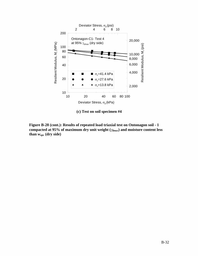
Deviator Stress, Vd (psi) 2 4 6 8 10
200
Re
silie
nt M
odu
lus,
Mr (
MP
a) 20,000
10 100 20 40 60 80
Deviator Stress, Vd (kPa)
Vc=41.4 kPa
Vc=27.6 kPa
Vc=13.8 kPa
Ontonagon-C1- Test 4 at 95% Jdmax (dry side)
100 80
10,000 60 8,000
6,000 40
Re
silie
nt M
odul
us, M
r (ps
i)
4,000
20
2,000
10
(c) Test on soil specimen #4
Figure B-28 (cont.): Results of repeated load triaxial test on Ontonagon soil - 1
compacted at 95% of maximum dry unit weight (Jdmax) and moisture content less
than wopt. (dry side)
B-32

Deviator Stress, Vd (psi)
2 4 6 8 10 200
20,000
10 100 20 40 60 80
Deviator Stress, Vd (kPa)
Vc=41.4 kPa
Vc=27.6 kPa
Vc=13.8 kPa
Ontonagon-C1- Test 1 at Jdmax and wopt.
Res
ilien
t Mod
ulus
, Mr (
MP
a)
Res
ilien
t Mod
ulus
, Mr (
MP
a)
100 80
10,000 60 8,000
40 6,000
4,000
Re
silie
nt M
odul
us, M
r (ps
i)
Re
silie
nt M
odul
us, M
r (ps
i)
20
2,000
10
(a) Test on soil specimen #1
Deviator Stress, Vd (psi)
2 4 6 8 10 200
20000
10 100 20 40 60 80
Deviator Stress, Vd (kPa)
Vc=41.4 kPa
Vc=27.6 kPa
Vc=13.8 kPa
Ontonagon-C1- Test 2 at Jdmax and wopt.
100 80
10000 60 8000
6000
4000
40
20
2000
10
(b) Test on soil specimen #2
Figure B-29: Results of repeated load triaxial test on Ontonagon soil - 1 compacted
at maximum dry unit weight (Jdmax) and optimum moisture content (wopt.)
B-33

Deviator Stress, Vd (psi)
2 4 6 8 10 200
20,000
10 100 20 40 60 80
Deviator Stress, Vd (kPa)
Vc=41.4 kPa
Vc=27.6 kPa
Vc=13.8 kPa
Ontonagon-C1- Test 1 at 95% Jdmax (wet side)
Res
ilien
t Mod
ulus
, Mr (
MP
a)
Res
ilien
t Mod
ulus
, Mr (
MP
a)
100 80
Re
silie
nt M
odul
us, M
r (ps
i)
Re
silie
nt M
odul
us, M
r (ps
i)
10,000 60 8,000
6,000
4,000
40
20
2,000
10
(a) Test on soil specimen #1
Deviator Stress, Vd (psi)
2 4 6 8 10 200
20,000
10 100 20 40 60 80
Deviator Stress, Vd (kPa)
Vc=41.4 kPa
Vc=27.6 kPa
Vc=13.8 kPa
Ontonagon-C1- Test 2 at 95% Jdmax (wet side)
100 80
60
40
10,000 8,000
6,000
4,000
20
2,000
10
(b) Test on soil specimen #2
Figure B-30: Results of repeated load triaxial test on Ontonagon soil - 1 compacted
at 95% of maximum dry unit weight (Jdmax) and moisture content more than wopt.
(wet side)
B-34

Deviator Stress,Vd (psi)
2 4 6 8 10 200
Res
ilien
t Mod
ulus
, Mr (
MP
a) 20,000
10 10020 40 60 80
Deviator Stress,Vd (kPa)
Vc=41.4 kPa
Vc=27.6 kPa
Vc=13.8 kPa
Ontonagon-C2 - Test 1 at 95% Jdmax (dry side)
100 80
10,000 60 8,000
6,000 40
Re
silie
nt M
odul
us, M
r (ps
i)
4,000
20
2,000
10
(a) Test on soil specimen #1
Figure B-31: Results of repeated load triaxial test on Ontonagon soil - 2 compacted
at 95% of maximum dry unit weight (Jdmax) and moisture content less than wopt. (dry
side)
B-35
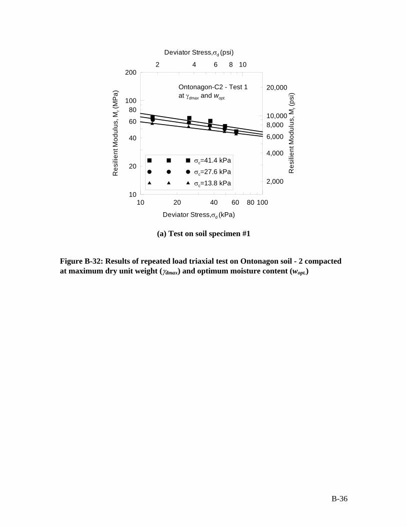
Deviator Stress,Vd (psi)
2 4 6 8 10 200
20,000
10 100 20 40 60 80
Deviator Stress,Vd (kPa)
Vc=41.4 kPa
Vc=27.6 kPa
Vc=13.8 kPa
Ontonagon-C2 - Test 1 at Jdmax and wopt.
Res
ilien
t Mod
ulus
, Mr (
MP
a)
100 80
Re
silie
nt M
odul
us, M
r (ps
i)
10,000 60 8,000
6,000
4,000
40
20
2,000
10
(a) Test on soil specimen #1
Figure B-32: Results of repeated load triaxial test on Ontonagon soil - 2 compacted
at maximum dry unit weight (Jdmax) and optimum moisture content (wopt.)
B-36

Deviator Stress,Vd (psi)
2 4 6 8 10 200
20,000
10 10020 40 60 80
Deviator Stress,Vd (kPa)
Vc=41.4 kPa
Vc=27.6 kPa
Vc=13.8 kPa
Ontonagon-C2 - Test 1 at 95% Jdmax (wet side)
Res
ilien
t Mod
ulus
, Mr (
MP
a)
100 80
60
40
Re
silie
nt M
od
ulus
, Mr (
psi)
10,000 8,000
6,000
4,000
20
2,000
10
(a) Test on soil specimen #1
Figure B-33: Results of repeated load triaxial test on Ontonagon soil - 2 compacted
at 95% of maximum dry unit weight (Jdmax) and moisture content more than wopt.
(wet side)
B-37
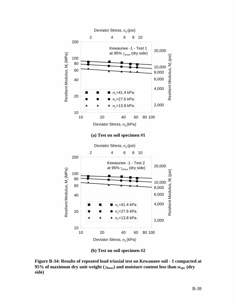
Deviator Stress, Vd (psi)
2 4 6 8 10 200
20,000
10 100 20 40 60 80
Deviator Stress, Vd (kPa)
Vc=41.4 kPa
Vc=27.6 kPa
Vc=13.8 kPa
Kewaunee -1 - Test 1 at 95% Jdmax (dry side)
Res
ilien
t Mod
ulus
, Mr (
MP
a)
Res
ilien
t Mod
ulus
, Mr (
MP
a)
100 80
10,000 60 8,000
40 6,000
4,000
Re
silie
nt M
odul
us, M
r (ps
i)
Re
silie
nt M
odul
us, M
r (ps
i)
20
2,000
10
(a) Test on soil specimen #1
Deviator Stress, Vd (psi)
2 4 6 8 10 200
20,000
10 100 20 40 60 80
Deviator Stress, Vd (kPa)
Vc=41.4 kPa
Vc=27.6 kPa
Vc=13.8 kPa
Kewaunee -1 - Test 2 at 95% Jdmax (dry side)
100 80
10,000 60 8,000
6,000 40
4,000
20
2,000
10
(b) Test on soil specimen #2
Figure B-34: Results of repeated load triaxial test on Kewaunee soil - 1 compacted at
95% of maximum dry unit weight (Jdmax) and moisture content less than wopt. (dry
side)
B-38

Deviator Stress, Vd (psi)
2 4 6 8 10 200
20,000
10 100 20 40 60 80
Deviator Stress, Vd (kPa)
Vc=41.4 kPa
Vc=27.6 kPa
Vc=13.8 kPa
Kewaunee - 1 - Test 1 at Jdmax and wopt.
Res
ilien
t Mod
ulus
, Mr (
MP
a)
Res
ilien
t Mod
ulus
, Mr (
MP
a)
100 80
10,000 60 8,000
40 6,000
4,000
Re
silie
nt M
od
ulus
, Mr (
psi)
R
esi
lient
Mod
ulus
, Mr (
psi)
20
2,000
10
(a) Test on soil specimen #1
Deviator Stress, Vd (psi)
2 4 6 8 10 200
20,000
10 100 20 40 60 80
Deviator Stress, Vd (kPa)
Vc=41.4 kPa
Vc=27.6 kPa
Vc=13.8 kPa
Kewaunee -1 - Test 2 at Jdmax and wopt.
100 80
10,000 60 8,000
6,000
4,000
40
20
2,000
10
(b) Test on soil specimen #2
Figure B-35: Results of repeated load triaxial test on Kewaunee soil - 1 compacted at
maximum dry unit weight (Jdmax) and optimum moisture content (wopt.)
B-39

Deviator Stress, Vd (psi)
2 4 6 8 10 200
20,000
10 10020 40 60 80
Deviator Stress, Vd (kPa)
Vc=41.4 kPa
Vc=27.6 kPa
Vc=13.8 kPa
Kewaunee - 1 - Test 1 at 95% Jdmax (wet side)
Res
ilien
t Mod
ulus
, Mr (
MP
a)
Res
ilien
t Mod
ulus
, Mr (
MP
a)
100 80
Re
silie
nt M
od
ulus
, Mr (
psi)
R
esi
lient
Mo
dul
us, M
r (ps
i)
10,000 60 8,000
6,000
4,000
40
20
2,000
10
(a) Test on soil specimen #1
Deviator Stress, Vd (psi)
2 4 6 8 10 200
20,000
10 100 20 40 60 80
Deviator Stress, Vd (kPa)
Vc=41.4 kPa
Vc=27.6 kPa
Vc=13.8 kPa
Kewaunee - 1 - Test 2 at 95% Jdmax (wet side)
100 80
10,000 60 8,000
6,000
4,000
40
20
2,000
10
(b) Test on soil specimen #2
Figure B-36: Results of repeated load triaxial test on Kewaunee soil -1 compacted at
95% of maximum dry unit weight (Jdmax) and moisture content more than wopt. (wet
side)
B-40
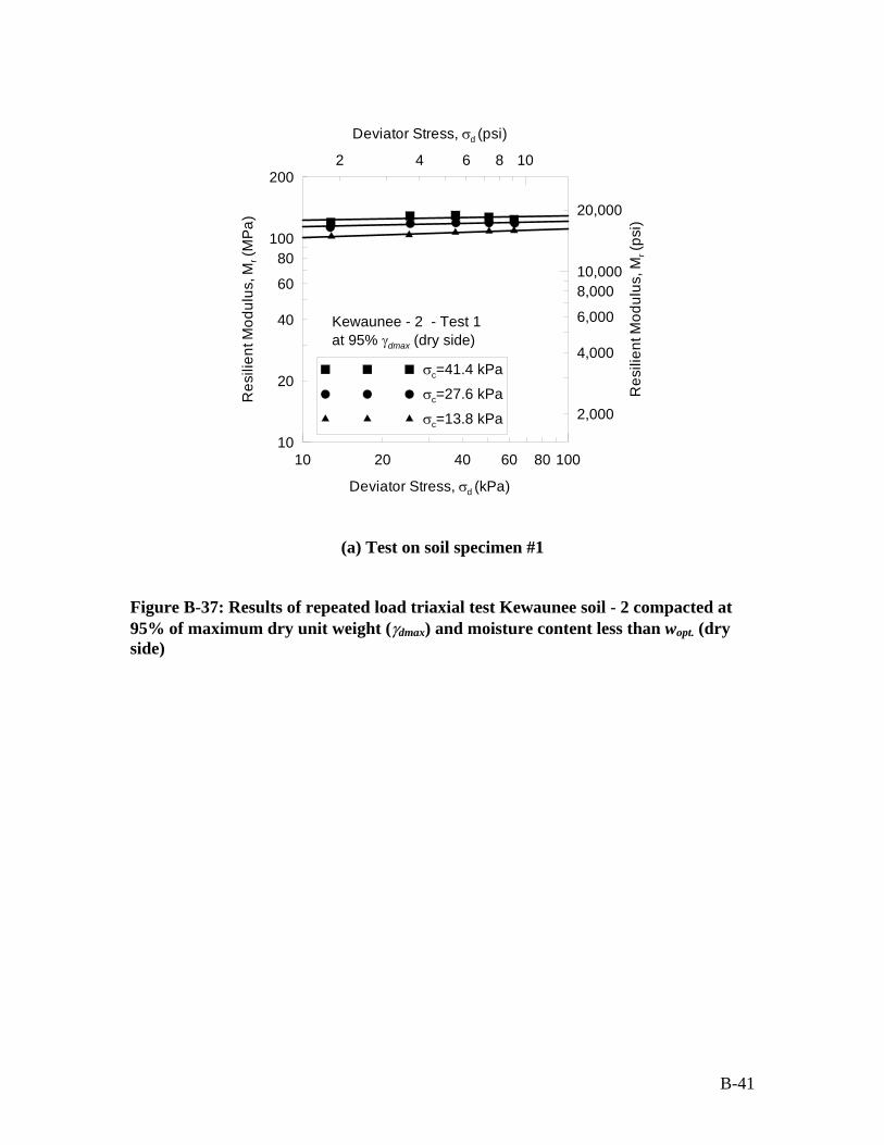
Deviator Stress, Vd (psi)
2 4 6 8 10 200
20,000
100 80
10,000 60 8,000
10 100 20 40 60 80
Deviator Stress, Vd (kPa)
Vc=41.4 kPa
Vc=27.6 kPa
Vc=13.8 kPa
Kewaunee - 2 - Test 1 at 95% Jdmax (dry side)
Res
ilien
t Mod
ulus
, Mr (
MP
a)
Res
ilien
t Mod
ulus
, Mr (
psi)
40 6,000
4,000
20
2,000
10
(a) Test on soil specimen #1
Figure B-37: Results of repeated load triaxial test Kewaunee soil - 2 compacted at
95% of maximum dry unit weight (Jdmax) and moisture content less than wopt. (dry
side)
B-41

Deviator Stress, Vd (psi)
2 4 6 8 10
10
100
20
40
60
80
200
Res
ilien
t Mod
ulus
, Mr (
MP
a)
10,000
20,000
8,000
6,000
4,000
2,000
Re
silie
nt M
odul
us, M
r (ps
i)
Vc=41.4 kPa
Vc=27.6 kPa
Vc=13.8 kPa
Kewaunee - 2 - Test 1 at Jdmax and wopt.
Res
ilien
t Mod
ulus
, Mr (
MP
a)
10 20 40 60 80 100
Deviator Stress, Vd (kPa)
(a) Test on soil specimen #1
Deviator Stress, Vd (psi)
2 4 6 8 10 200
20,000
100 80
10,000 60 8,000
10 100 20 40 60 80
Deviator Stress, Vd (kPa)
6,000
4,000
2,000
Vc=41.4 kPa
Vc=27.6 kPa
Vc=13.8 kPa
Kewaunee - 2 - Test 2 at Jdmax and wopt.
40
20
Res
ilien
t Mod
ulus
, Mr (
psi)
10
(b) Test on soil specimen #2
Figure B-38: Results of repeated load triaxial test on Kewaunee soil - 2 compacted at
maximum dry unit weight (Jdmax) and optimum moisture content (wopt.)
B-42

Deviator Stress, Vd (psi)
2 4 6 8 10 200
20,000
10 100 20 40 60 80
Deviator Stress, Vd (kPa)
Vc=41.4 kPa
Vc=27.6 kPa
Vc=13.8 kPa
Kewaunee - 2 - Test 1 at 95% Jdmax (wet side)
Res
ilien
t Mod
ulus
, Mr (
MP
a)
100 80
Re
silie
nt M
odul
us, M
r (ps
i)
10,000 60 8,000
6,000
4,000
40
20
2,000
10
(a) Test on soil specimen #1
Figure B-39: Results of repeated load triaxial test on Kewaunee soil - 2 compacted at
95% of maximum dry unit weight (Jdmax) and moisture content more than wopt. (wet
side)
B-43

Deviator Stress, Vd (psi)
2 4 6 8 10
10
100
20
40
60
80
200
Res
ilien
t Mod
ulus
, Mr (
MP
a)
10,000
20,000
8,000
6,000
4,000
2,000
Res
ilien
t Mod
ulus
, Mr (
psi)
Vc=41.4 kPa
Vc=27.6 kPa
Vc=13.8 kPa
Shiocton - Test 1 at Jdmax and wopt.
10 20 40 60 80 100
Deviator Stress, Vd (kPa)
(a) Test on soil specimen #1
Deviator Stress, Vd (psi)
2 4 6 8 10
10 100 20 40 60 80
Deviator Stress, Vd (kPa)
10
100
20
40
60
80
200
Res
ilien
t Mod
ulus
, Mr (
MP
a)
10,000
20,000
8,000
6,000
4,000
2,000
Re
silie
nt M
odul
us, M
r (ps
i)
Vc=41.4 kPa
Vc=27.6 kPa
Vc=13.8 kPa
Shiocton - Test 2 at Jdmax and wopt.
(b) Test on soil specimen #2
Figure B-40: Results of repeated load triaxial test on Shiocton soil compacted at
maximum dry unit weight (Jdmax) and optimum moisture content (wopt.)
B-44

Deviator Stress, Vd (psi)
2 4 6 8 10
10
100
20
40
60
80
200
Res
ilien
t Mod
ulus
, Mr (
MP
a)
10,000
20,000
8,000
6,000
4,000
2,000
Re
silie
nt M
odul
us, M
r (ps
i)
Vc=41.4 kPa
Vc=27.6 kPa
Vc=13.8 kPa
Shiocton - Test 1 at 95% Jdmax (wet side)
10 20 40 60 80 100
Deviator Stress, Vd (kPa)
(a) Test on soil specimen #1
Deviator Stress, Vd (psi)
2 4 6 8 10
10 100 20 40 60 80
Deviator Stress, Vd (kPa)
10
100
20
40
60
80
200
Res
ilien
t Mod
ulus
, Mr (
MP
a)
10,000
20,000
8,000
6,000
4,000
2,000
Re
silie
nt M
odul
us, M
r (ps
i)
Vc=41.4 kPa
Vc=27.6 kPa
Vc=13.8 kPa
Shiocton - Test 2 at 95% Jdmax (wet side)
(b) Test on soil specimen #2
Figure B-41: Results of repeated load triaxial test on Shiocton soil compacted at
95% of maximum dry unit weight (Jdmax) and moisture content more than wopt. (wet
side)
B-45

Deviator Stress, Vd (psi)
2 4 6 8 10
10
100
20
40
60
80
200
Res
ilien
t Mod
ulus
, Mr (
MP
a)
10,000
20,000
8,000
6,000
4,000
2,000
Res
ilien
t Mod
ulus
, Mr (
psi)
Vc=41.4 kPa
Vc=27.6 kPa
Vc=13.8 kPa
Withee - Test 1 at 95% Jdmax (dry side)
10 20 40 60 80 100
Deviator Stress, Vd (kPa)
(a) Test on soil specimen #1
Deviator Stress, Vd (psi)
2 4 6 8 10
10 100 20 40 60 80
Deviator Stress, Vd (kPa)
10
100
20
40
60
80
200
Res
ilien
t Mod
ulus
, Mr (
MP
a)
10,000
20,000
8,000
6,000
4,000
2,000
Re
silie
nt M
odul
us, M
r (ps
i)
Vc=41.4 kPa
Vc=27.6 kPa
Vc=13.8 kPa
Withee - Test 2 at 95% Jdmax (dry side)
(b) Test on soil specimen #2
Figure B-42: Results of repeated load triaxial test on Withee soil compacted at 95%
of maximum dry unit weight (Jdmax) and moisture content less than wopt. (dry side)
B-46
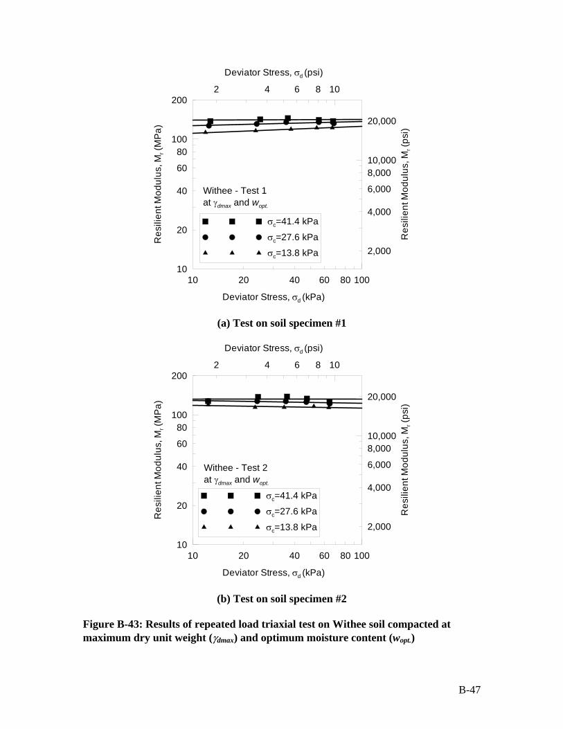
Deviator Stress, Vd (psi)
2 4 6 8 10
10
100
20
40
60
80
200
Res
ilien
t Mod
ulus
, Mr (
MP
a)
10,000
20,000
8,000
6,000
4,000
2,000
Res
ilien
t Mod
ulus
, Mr (
psi)
Vc=41.4 kPa
Vc=27.6 kPa
Vc=13.8 kPa
Withee - Test 1 at Jdmax and wopt.
10 20 40 60 80 100
Deviator Stress, Vd (kPa)
(a) Test on soil specimen #1
Deviator Stress, Vd (psi)
2 4 6 8 10
10 100 20 40 60 80
Deviator Stress, Vd (kPa)
10
100
20
40
60
80
200
Res
ilien
t Mod
ulus
, Mr (
MP
a)
10,000
20,000
8,000
6,000
4,000
2,000
Res
ilien
t Mod
ulus
, Mr (
psi)
Vc=41.4 kPa
Vc=27.6 kPa
Vc=13.8 kPa
Withee - Test 2 at Jdmax and wopt.
(b) Test on soil specimen #2
Figure B-43: Results of repeated load triaxial test on Withee soil compacted at
maximum dry unit weight (Jdmax) and optimum moisture content (wopt.)
B-47

Deviator Stress, Vd (psi)
2 4 6 8 10
10
100
20
40
60
80
200
Res
ilien
t Mod
ulus
, Mr (
MP
a)
10,000
20,000
8,000
6,000
4,000
2,000
Res
ilien
t Mod
ulus
, Mr (
psi)
Vc=41.4 kPa
Vc=27.6 kPa
Vc=13.8 kPa
Withee - Test 1 at 95% Jdmax (wet side)
10 20 40 60 80 100
Deviator Stress, Vd (kPa)
(a) Test on soil specimen #1
Deviator Stress, Vd (psi)
2 4 6 8 10
10 100 20 40 60 80
Deviator Stress, Vd (kPa)
10
100
20
40
60
80
200
Res
ilien
t Mod
ulus
, Mr (
MP
a)
10,000
20,000
8,000
6,000
4,000
2,000
Res
ilien
t Mod
ulus
, Mr (
psi)
Vc=41.4 kPa
Vc=27.6 kPa
Vc=13.8 kPa
Withee - Test 2 at 95% Jdmax (wet side)
(b) Test on soil specimen #2
Figure B-44: Results of repeated load triaxial test on Withee soil compacted at 95%
of maximum dry unit weight (Jdmax) and moisture content more than wopt. (wet side)
B-48

Deviator Stress, Vd (psi)
2 4 6 8 10
10
100
20
40
60
80
200
Res
ilien
t Mod
ulus
, Mr (
MP
a)
10,000
20,000
8,000
6,000
4,000
2,000
Res
ilien
t Mod
ulus
, Mr (
psi)
Vc=41.4 kPa
Vc=27.6 kPa
Vc=13.8 kPa
Eleva - Test 1 at 95% Jdmax (dry side)
10 20 40 60 80 100
Deviator Stress, Vd (kPa)
(a) Test on soil specimen #1
Deviator Stress, Vd (psi)
2 4 6 8 10
10 100 20 40 60 80
Deviator Stress, Vd (kPa)
10
100
20
40
60
80
200
Res
ilien
t Mod
ulus
, Mr (
MP
a)
10,000
20,000
8,000
6,000
4,000
2,000
Res
ilien
t Mod
ulus
, Mr (
psi)
Vc=41.4 kPa
Vc=27.6 kPa
Vc=13.8 kPa
Eleva - Test 2 at 95% Jdmax (dry side)
(b) Test on soil specimen #2
Figure B-45: Results of repeated load triaxial test on Eleva soil compacted at 95% of
maximum dry unit weight (Jdmax) and moisture content less than wopt. (dry side)
B-49
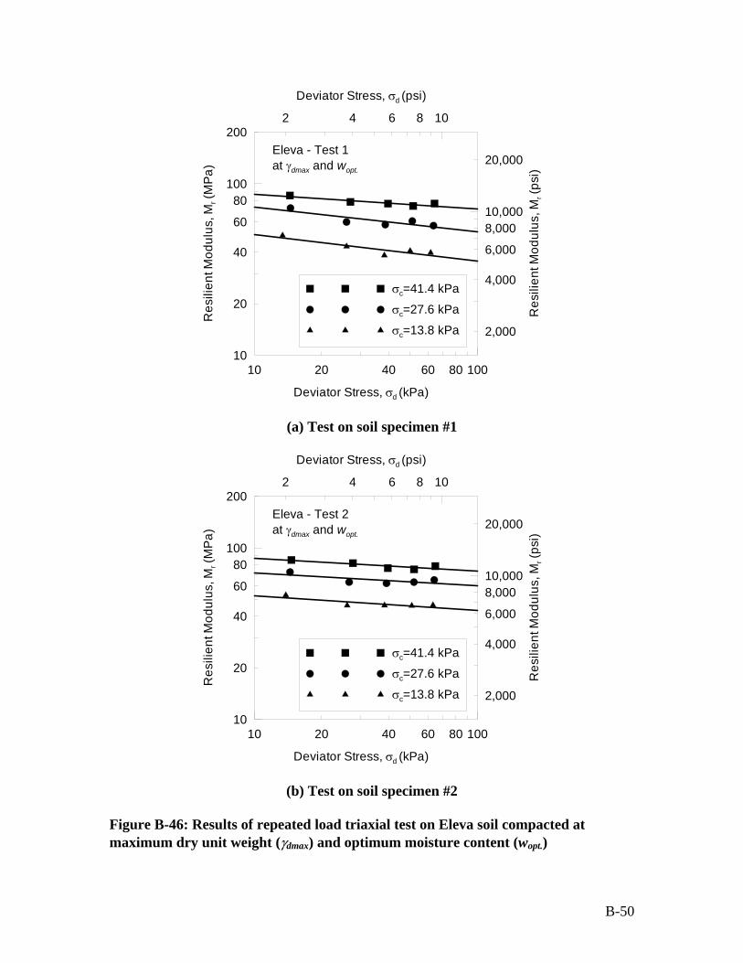
Deviator Stress, Vd (psi)
2 4 6 8 10
10
100
20
40
60
80
200
Res
ilien
t Mod
ulus
, Mr (
MP
a)
10,000
20,000
8,000
6,000
4,000
2,000
Res
ilien
t Mod
ulus
, Mr (
psi)
Vc=41.4 kPa
Vc=27.6 kPa
Vc=13.8 kPa
Eleva - Test 1 at Jdmax and wopt.
10 20 40 60 80 100
Deviator Stress, Vd (kPa)
(a) Test on soil specimen #1
Deviator Stress, Vd (psi)
2 4 6 8 10
10 100 20 40 60 80
Deviator Stress, Vd (kPa)
10
100
20
40
60
80
200
Res
ilien
t Mod
ulus
, Mr (
MP
a)
10,000
20,000
8,000
6,000
4,000
2,000
Res
ilien
t Mod
ulus
, Mr (
psi)
Vc=41.4 kPa
Vc=27.6 kPa
Vc=13.8 kPa
Eleva - Test 2 at Jdmax and wopt.
(b) Test on soil specimen #2
Figure B-46: Results of repeated load triaxial test on Eleva soil compacted at
maximum dry unit weight (Jdmax) and optimum moisture content (wopt.)
B-50

Deviator Stress, Vd (psi)
2 4 6 8 10
10
100
20
40
60
80
200
Res
ilien
t Mod
ulus
, Mr (
MP
a)
10,000
20,000
8,000
6,000
4,000
2,000
Res
ilien
t Mod
ulus
, Mr (
psi)
Vc=41.4 kPa
Vc=27.6 kPa
Vc=13.8 kPa
Eleva - Test 1 at 95% Jdmax (wet side)
10 20 40 60 80 100
Deviator Stress, Vd (kPa)
(a) Test on soil specimen #1
Deviator Stress, Vd (psi)
2 4 6 8 10
10 100 20 40 60 80
Deviator Stress, Vd (kPa)
10
100
20
40
60
80
200
Res
ilien
t Mod
ulus
, Mr (
MP
a)
10,000
20,000
8,000
6,000
4,000
2,000
Res
ilien
t Mod
ulus
, Mr (
psi)
Vc=41.4 kPa
Vc=27.6 kPa
Vc=13.8 kPa
Eleva - Test 2 at 95% Jdmax (wet side)
(b) Test on soil specimen #2
Figure B-47: Results of repeated load triaxial test on Eleva soil compacted at 95% of
maximum dry unit weight (Jdmax) and moisture content more than wopt. (wet side)
B-51