Determination of thermodynamic properties of liquid Ag-In, Ag-Sb, Ag-Sn, In-Sb, Sb-Sn, Ag-In-Sb,...
27
Determination of thermodynamic properties of liquid Ag-In, Ag-Sb, Ag-Sn, In-Sb, Sb-Sn, Ag-In-Sb, Cu-In-Sn and Ag-In-Sn systems by Knudsen effusion Mass Spectrometry A. Popovic and L. Bencze* Jozef Stefan Institute, Jamova 39, SLO-1000 Ljubljana, Slovenia. *Eötvös Loránd University, Dept. of Physical Chemistry, H-1117 Budapest, Pázmány Péter sétány 1/A, Hungary
-
date post
19-Dec-2015 -
Category
Documents
-
view
229 -
download
1
Transcript of Determination of thermodynamic properties of liquid Ag-In, Ag-Sb, Ag-Sn, In-Sb, Sb-Sn, Ag-In-Sb,...

Determination of thermodynamic properties of liquid Ag-In, Ag-Sb, Ag-Sn, In-Sb, Sb-Sn, Ag-In-Sb, Cu-In-Sn
and Ag-In-Sn systems by Knudsen effusion Mass Spectrometry
A. Popovic and L. Bencze*
Jozef Stefan Institute, Jamova 39, SLO-1000 Ljubljana, Slovenia.
*Eötvös Loránd University, Dept. of Physical Chemistry, H-1117 Budapest, Pázmány Péter sétány 1/A, Hungary

The scheme of a Knudsen cell - mass spectrometer system (FZ Jülich, Germany)
< 20 KEMS laboratories over the world

ION SOURCE
The scheme of single and double the Knudsen cells.

Determination of equilibrium vapour pressure by KEMS:
iii
ij
i totj,ii
ij
totj,j a
IKTIKTp
Inghram, Chupka, 1955
where K is the (general) instrumental sensitivity constant Iij is the intensity of ion i originating from neutral species j i is the isotopic abundance of ion i
i is the multiplier gain factor of ion i (sensitivity constant of the detector for ion i) - in multiplier current measurement mode only ai is the (spectral) abundance of ion i in the mass spectrum i is the total ionisation cross section of species j at the actual electron energy (si depends on j and the ionising electron energy)
K can be determined by calibration using e.g. a reference substance (e.g.pure component) in the next or previous experiment, using internal standard inside the same cell, using isothermal long-term evaporation etc).
*j
jj p
pa pj*: pressure over
the pure component

Determination of activities by KEMS:
1/ by direct pressure calibration (DPC) using pure metals as reference substances in subsequent experiments (the uncertainty can reach as high as 20% due to a the change of sensitivity constant day-by-day),
2/ using a proper internal standard (ISM) being in the same cell,
3/ using twin or multiple Knudsen cell technique (MKC) (some of the compartments are filled with the pure components),
4/ from the change of the oligomer (monomer, dimer, trimer etc.) composition in the vapour (this latter method can be applied in the only case if the metals vaporise in the form of oligomers, such as Sb(g), Sb2 (g), Sb3(g), Sb4 (g)),
5/ applying the mass spectrometric Gibbs-Duhem Ion Intensity Ratio Method (GD- IIRM) that is a modification of the well-known Gibbs-Duhem relationship with MS quantities (i.e. ion intensities),
6/ applying the isothermal evaporation method (IEM) /long-term or total/,---------------------------------------------------------------------------------------------------------------------7/ for ternary alloys, by applying Miki’ s or Tomiska’ s new KEMS methods for the determination of the constants in the power series expression of GE. (Miki: Redlich-Kister expression, Tomiska: TAP expression)
*jjj pap

THERMODYNAMIC PROPERTIES OF MIXING
Activities and the activity coefficients ---> chemical potential change of mixing, excess chemical potential ---->Gibbs energy change of mixing, excess Gibbs energy
The uncertainty of Ei /(E
i)/ is usually lower than +-1 kJ/mol (at 1400 K, assuming an error as factor 1.1 in the values of activities, =1.11 kJ/mol is obtained).--------------------------------------------------------------------------------------Temperature dependence of activities---> partial and integral enthalpy changes of mixing.
Uncertainties: (HEi )~1-2 kJ/mol for partial quantities but in case of
wrong identification of the composition the uncertainty of the integral quantity (HE) can reach as high as ~10 kJ/mol if the partial quantities depend on composition very sharply. The Gibbs-Duhem integration helps against this problem.

0.30 0.35 0.40 0.45 0.50
-70000
-60000
-50000
-40000
-30000
this work, GD this work, GD-IIR this work, direct calibr.
referencecomposition
fH
m/J
.mo
l-1
cAl
AlcFe
0.5(1-c)Ni
0.5(1-c)
Al-Fe-Ni
BINARY SYSTEMS
0.0 0.2 0.4 0.6 0.8 1.0
-7000
-6000
-5000
-4000
-3000
-2000
-1000
0
COST
Moser et al.
Jendrzejczyk et al.
this work
Qi et al.
Ag-In, 1200 K
GE/(
J.m
ol-1)
XAg

0.0 0.2 0.4 0.6 0.8 1.0
-4000
-3000
-2000
-1000
0
Xie et al.
Kato et al.
Oh et al. /COST/
Chevalier et al.
this work
Ag-Sn, 1300 K
G
E/(
J.m
ol-1)
XAg

0.0 0.2 0.4 0.6 0.8 1.0
-6000
-5000
-4000
-3000
-2000
-1000
0
Hultgren(+-840)
this work
Krzyzak et al.
Ag-Sb, 1250 K
G
E/(
J.m
ol-1)
XSb
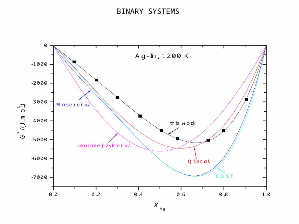
0.0 0.2 0.4 0.6 0.8 1.0
-4000
-3000
-2000
-1000
0
Ansara et al.
this work
In-Sb, 950 K
G
E/(
J.m
ol-1)
XSb
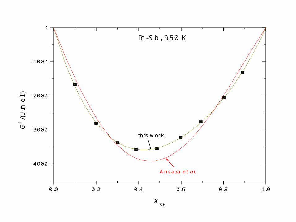
0.0 0.2 0.4 0.6 0.8 1.0
-9000
-8000
-7000
-6000
-5000
-4000
-3000
-2000
-1000
0
In(l) + Sb(l) = InSb(l) rHo=-12.0 kJ/mol
3 In(l) + Sb(l) = In3Sb(l)
rHo=-16.8 kJ/mol
directly measured fitted to IAMT model
In-Sb, 950 K
m
ixG
/(J.
mo
l-1)
XSb

0.0 0.2 0.4 0.6 0.8 1.0-3000
-2000
-1000
0
Jansson et al.
this work
Sb-Sn, 905 K
G
E/(
J.m
ol-1)
XSb

)]1()[1(
)]12()[1(
])12()12()[1(
])()([
InCu2
n CuInSIn1
n CuInSCu0
n CuInSInCuInCu
CuIn1InSn
0InSnInCuIn
2InCu
2CuSnInCu
1CuSn
0CuSnInCuCu
2InCu
2CuInInCu
1CuIn
0CuInInCu
E
XXLXLXLXXXX
XXLLXXX
XXLXXLLXXX
XXLXXLLXXG
Miki’s method supplemented by us for the calculation of all the 3 ternary L’s:
where GE is the excess Gibbs free energy, expressed in terms of binary and ternary interaction parameters.
YXXXXL
XXXLXXXXLX
G
InSnCuSn2
n CuInS
2InCuSn
1n CuInSInCuCuSn
0n CuInS
InCu
E
)2(
))(()2(
where
)]223([
)]12(42)[1(
])12()12()[21(
)](2[
])()([{
InIn1InSn
0InSnIn
InCu2CuSn
1CuSnCuInCu
2InCu
2CuSnInCu
1CuSn
0CuSnCuIn
InCu2CuIn
1CuInInCu
2InCu
2CuInInCu
1CuIn
0CuInIn
XXLLX
XXLLXXX
XXLXXLLXX
XXLLXX
XXLXXLLXY
ClnlnRCuSn
SnCu
Sn
Cu
InCu
E
XI
XIRTT
X
G
where ICu / ISn is the measured ion intensity ratio of Cu+ to Sn + and C is a constant
Redlich-Kister-Muggianu:

CuSn
SnCulnXI
XIRTYY YYYYsumma
By rearranging and putting similar terms together we finally get that :
InSnCuSn2
n CuInS
2InCuSn
1n CuInSInCuCuSn
0n CuInS
)2(
))(()2(-C
XXXXL
XXXLXXXXLYsumma
The three ternary parameters can finally be found by solving the set of linear equations:
nnn XXXXXXXXXXX
XXXXXXXXXXX
XXXXXXXXXXX
InSnCuSn2InCuSnInCuCuSn
2InSnCuSn22InCuSn2InCuCuSn
1InSnCuSn12InCuSn1InCuCuSn
221
221
221
2CuInSn
1CuInSn
0CuInSn
L
L
L
C
nYsumma
Ysumma
Ysumma
2
1
where ’n’ is the number of the measured compositions. If n>4 the solution of the linear equation system should be replaced with a multiple regression problem.
The method provides the three ternary parameters, and, as input parameters it needs the binary parameters (either from own experiments or from literature) and the measured ion intensity ratio at various compositions for the given temperature. Any ion intensity ratio can be used from the total 3 variations of a ternary systems.

)ln(5.1)(89.0-42.3)726.8(7057)-59473(0 TTTL
)ln(9.1)(14.9-75.1)(40.412518)139125(1 TTTL
)ln(4.1)(51.733.8)436.6(5633)-111387(2 TTTL
The result for Cu-In-Sn, obtained from ICu / ISn of 23 compositions, is as follows:
0.0 0.1 0.2 0.3 0.4 0.5 0.6 0.7 0.8 0.9 1.0
0.0
0.1
0.2
0.3
0.4
0.5
0.6
0.7
0.8
0.9
1.0 0.0
0.1
0.2
0.3
0.4
0.5
0.6
0.7
0.8
0.9
1.0
Cu
Sn
In
Fig1. Measured compositions.

700 800 900 1000 1100 1200 1300 1400 1500
-100
-50
0
50
100
-C
L2
L1
L0
measured temp. range
kJ/m
ole
Temperature /K
700 800 900 1000 1100 1200 1300 1400 1500
-100
-50
0
50
100
L2
L1L
0
kJ/m
ole
Temperature /K
Fig.2. Ternary parameters as a functionof temperature, obtained in this work.
Fig.3. Ternary parameters as a functionof temperature by Liu et al..

0.0 0.2 0.4 0.6 0.8 1.00.0
0.2
0.4
0.6
0.8
1.0
Raoult's line
Cu-In-Sn system at 1173K Cu/Sn=1 section
solid line: RKM model with KEMS measured ion int. ratiosdashed line: calculated using Liu's ternary parameters (RKM)circle: measured data (EMF) from Yamaguchi at 1200Ktriangle: KEMS (simple mass loss by evaporation)
act
ivity
of
In
mole fraction of In
Fig. 4. Comparison of indium activity data obtained from our own and Liu’ s ternary parameters, from our measured mass loss data and from the measured EMF data of Yamaguchi.

Fig.5. Comparison of the partial excess enthalpy of indium obtained from our own and Liu’ s ternary parameters, from the ion intensity of In vs. temperature directly and by assuming binary parameters only.
0.0 0.2 0.4 0.6 0.8 1.0
-10000
-5000
0
5000
10000
15000
20000
25000
30000
35000
KEMS + RKM model, only binary interaction assumed
Liu et al.
KEMS+RKM modelternary interactionalso assumed
'pure' KEMS (this work)
Cu/Sn=1T=1173K
HIn
E/(
J.m
ol-1
)
mole fraction of Indium
0.00 0.25 0.50 0.75 1.00
0.00
0.25
0.50
0.75
1.00 0.0
0.2
0.4
0.6
0.8
1.0
Cu
InSn 0.00 0.25 0.50 0.75 1.00
0.00
0.25
0.50
0.75
1.00 0.0
0.2
0.4
0.6
0.8
1.0
-5000
-4000
0.00 0.25 0.50 0.75 1.00
0.00
0.25
0.50
0.75
1.00 0.0
0.2
0.4
0.6
0.8
1.0
-3000
0.00 0.25 0.50 0.75 1.00
0.00
0.25
0.50
0.75
1.00 0.0
0.2
0.4
0.6
0.8
1.0
-2000
0.00 0.25 0.50 0.75 1.00
0.00
0.25
0.50
0.75
1.00 0.0
0.2
0.4
0.6
0.8
1.0
-1000
0.00 0.25 0.50 0.75 1.00
0.00
0.25
0.50
0.75
1.00 0.0
0.2
0.4
0.6
0.8
1.0
-500
0.00 0.25 0.50 0.75 1.00
0.00
0.25
0.50
0.75
1.00 0.0
0.2
0.4
0.6
0.8
1.0
00.00 0.25 0.50 0.75 1.00
0.00
0.25
0.50
0.75
1.00 0.0
0.2
0.4
0.6
0.8
1.0
-4500
0.00 0.25 0.50 0.75 1.00
0.00
0.25
0.50
0.75
1.00 0.0
0.2
0.4
0.6
0.8
1.0
-100
0.00 0.25 0.50 0.75 1.00
0.00
0.25
0.50
0.75
1.00 0.0
0.2
0.4
0.6
0.8
1.0
-5000
0.00 0.25 0.50 0.75 1.00
0.00
0.25
0.50
0.75
1.00 0.0
0.2
0.4
0.6
0.8
1.0
-4500
0.00 0.25 0.50 0.75 1.00
0.00
0.25
0.50
0.75
1.00 0.0
0.2
0.4
0.6
0.8
1.0
-4000
0.00 0.25 0.50 0.75 1.00
0.00
0.25
0.50
0.75
1.00 0.0
0.2
0.4
0.6
0.8
1.0
-3000
0.00 0.25 0.50 0.75 1.00
0.00
0.25
0.50
0.75
1.00 0.0
0.2
0.4
0.6
0.8
1.0
-2000
0.00 0.25 0.50 0.75 1.00
0.00
0.25
0.50
0.75
1.00 0.0
0.2
0.4
0.6
0.8
1.0
-1000
0.00 0.25 0.50 0.75 1.00
0.00
0.25
0.50
0.75
1.00 0.0
0.2
0.4
0.6
0.8
1.0
-500
0.00 0.25 0.50 0.75 1.00
0.00
0.25
0.50
0.75
1.00 0.0
0.2
0.4
0.6
0.8
1.0
Sn In
Cu
-100
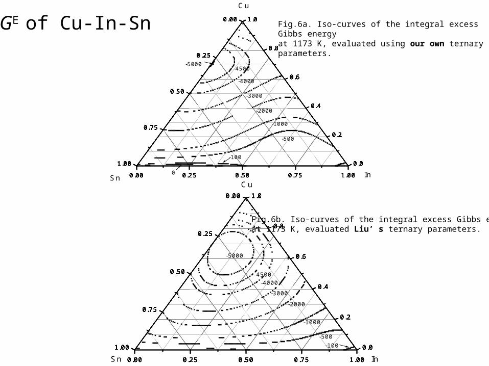
Fig.6a. Iso-curves of the integral excess Gibbs energy at 1173 K, evaluated using our own ternary parameters.
Fig.6b. Iso-curves of the integral excess Gibbs energy at 1173 K, evaluated Liu’ s ternary parameters.
GE of Cu-In-Sn

0.00 0.25 0.50 0.75 1.00
0.00
0.25
0.50
0.75
1.00 0.0
0.2
0.4
0.6
0.8
1.0
0.00 0.25 0.50 0.75 1.00
0.00
0.25
0.50
0.75
1.00 0.0
0.2
0.4
0.6
0.8
1.0
0.00 0.25 0.50 0.75 1.00
0.00
0.25
0.50
0.75
1.00 0.0
0.2
0.4
0.6
0.8
1.0
0.00 0.25 0.50 0.75 1.00
0.00
0.25
0.50
0.75
1.00 0.0
0.2
0.4
0.6
0.8
1.0
0.00 0.25 0.50 0.75 1.00
0.00
0.25
0.50
0.75
1.00 0.0
0.2
0.4
0.6
0.8
1.0
0.00 0.25 0.50 0.75 1.00
0.00
0.25
0.50
0.75
1.00 0.0
0.2
0.4
0.6
0.8
1.0
0.00 0.25 0.50 0.75 1.00
0.00
0.25
0.50
0.75
1.00 0.0
0.2
0.4
0.6
0.8
1.0
0.00 0.25 0.50 0.75 1.00
0.00
0.25
0.50
0.75
1.00 0.0
0.2
0.4
0.6
0.8
1.0
0.00 0.25 0.50 0.75 1.00
0.00
0.25
0.50
0.75
1.00 0.0
0.2
0.4
0.6
0.8
1.0
0.00 0.25 0.50 0.75 1.00
0.00
0.25
0.50
0.75
1.00 0.0
0.2
0.4
0.6
0.8
1.0
0.00 0.25 0.50 0.75 1.00
0.00
0.25
0.50
0.75
1.00 0.0
0.2
0.4
0.6
0.8
1.0
0.00 0.25 0.50 0.75 1.00
0.00
0.25
0.50
0.75
1.00 0.0
0.2
0.4
0.6
0.8
1.0
0.00 0.25 0.50 0.75 1.00
0.00
0.25
0.50
0.75
1.00 0.0
0.2
0.4
0.6
0.8
1.0
0.00 0.25 0.50 0.75 1.00
0.00
0.25
0.50
0.75
1.00 0.0
0.2
0.4
0.6
0.8
1.0
0.00 0.25 0.50 0.75 1.00
0.00
0.25
0.50
0.75
1.00 0.0
0.2
0.4
0.6
0.8
1.0
0.00 0.25 0.50 0.75 1.00
0.00
0.25
0.50
0.75
1.00 0.0
0.2
0.4
0.6
0.8
1.0
0.00 0.25 0.50 0.75 1.00
0.00
0.25
0.50
0.75
1.00 0.0
0.2
0.4
0.6
0.8
1.0
0.00 0.25 0.50 0.75 1.00
0.00
0.25
0.50
0.75
1.00 0.0
0.2
0.4
0.6
0.8
1.0
0.00 0.25 0.50 0.75 1.00
0.00
0.25
0.50
0.75
1.00 0.0
0.2
0.4
0.6
0.8
1.0
0.00 0.25 0.50 0.75 1.00
0.00
0.25
0.50
0.75
1.00 0.0
0.2
0.4
0.6
0.8
1.0
Sn In
Cu
0.00 0.25 0.50 0.75 1.00
0.00
0.25
0.50
0.75
1.00 0.0
0.2
0.4
0.6
0.8
1.0
+1500
+1000
+500
-500-1000
-1500
-200
0
00
0
+2400
-300
0
Fig.7a. Iso-curves of the integral excess enthalpy at 1400 K, evaluated using our own ternary parameters.
0.00 0.25 0.50 0.75 1.00
0.00
0.25
0.50
0.75
1.00 0.0
0.2
0.4
0.6
0.8
1.0
0.00 0.25 0.50 0.75 1.00
0.00
0.25
0.50
0.75
1.00 0.0
0.2
0.4
0.6
0.8
1.0
0.00 0.25 0.50 0.75 1.00
0.00
0.25
0.50
0.75
1.00 0.0
0.2
0.4
0.6
0.8
1.0
-500
-500
0.00 0.25 0.50 0.75 1.00
0.00
0.25
0.50
0.75
1.00 0.0
0.2
0.4
0.6
0.8
1.0
0
0
0.00 0.25 0.50 0.75 1.00
0.00
0.25
0.50
0.75
1.00 0.0
0.2
0.4
0.6
0.8
1.0
+500
+500
0.00 0.25 0.50 0.75 1.00
0.00
0.25
0.50
0.75
1.00 0.0
0.2
0.4
0.6
0.8
1.0
+1000
0.00 0.25 0.50 0.75 1.00
0.00
0.25
0.50
0.75
1.00 0.0
0.2
0.4
0.6
0.8
1.0
+1500
0.00 0.25 0.50 0.75 1.00
0.00
0.25
0.50
0.75
1.00 0.0
0.2
0.4
0.6
0.8
1.0
+1700
0.00 0.25 0.50 0.75 1.00
0.00
0.25
0.50
0.75
1.00 0.0
0.2
0.4
0.6
0.8
1.0
0.00 0.25 0.50 0.75 1.00
0.00
0.25
0.50
0.75
1.00 0.0
0.2
0.4
0.6
0.8
1.0
0.00 0.25 0.50 0.75 1.00
0.00
0.25
0.50
0.75
1.00 0.0
0.2
0.4
0.6
0.8
1.0
0.00 0.25 0.50 0.75 1.00
0.00
0.25
0.50
0.75
1.00 0.0
0.2
0.4
0.6
0.8
1.0
0
0
0.00 0.25 0.50 0.75 1.00
0.00
0.25
0.50
0.75
1.00 0.0
0.2
0.4
0.6
0.8
1.0
0.00 0.25 0.50 0.75 1.00
0.00
0.25
0.50
0.75
1.00 0.0
0.2
0.4
0.6
0.8
1.0
-170
0
0.00 0.25 0.50 0.75 1.00
0.00
0.25
0.50
0.75
1.00 0.0
0.2
0.4
0.6
0.8
1.0
0.00 0.25 0.50 0.75 1.00
0.00
0.25
0.50
0.75
1.00 0.0
0.2
0.4
0.6
0.8
1.0
0.00 0.25 0.50 0.75 1.00
0.00
0.25
0.50
0.75
1.00 0.0
0.2
0.4
0.6
0.8
1.0
Sn
Cu
InXIn
Fig.7b. Iso-curves of the integral excess enthalpy at 1400 K, evaluated using Liu’ s ternary parameters
HE of Cu-In-Sn

0.00 0.25 0.50 0.75 1.00
0.00
0.25
0.50
0.75
1.00 0.0
0.2
0.4
0.6
0.8
1.0
AgIn
Sn

InSnAgSn2AgInSn
2InAgSn
1AgInSnInAgAgSn
0AgInSn)/SnAgInSn(Ag)/SnAgInSn(Ag
)2(
))(()2(-
XXXXL
XXXLXXXXLCYsumma
2SnAgIn
2AgInSn
InSnAgIn1AgInSnSnAgAgIn
0AgInSn)/InAgInSn(Ag)/InAgInSn(Ag
))((
)2()2(-
XXXL
XXXXLXXXXLCYsumma
Two possibilities for getting ternary L’s:
1:
2:
=
nnnXXXXXXXXXXX
XXXXXXXXXXX
XXXXXXXXXXX
InSnAgSn2InAgSnInAgAgSn
2InSnAgSn2
2InAgSn2InAgAgSn
1InSnAgSn1
2InAgSn1InAgAgSn
221
221
221
2CuInSn
1CuInSn
0CuInSn
L
L
L
C
nYsumma
Ysumma
Ysumma
2
1
1:
2:
nnnXXXXXXXXXXX
XXXXXXXXXXX
XXXXXXXXXXX
2SnAgInInSnAgInSnAgAgIn
2
2SnAgIn2InSnAgIn2SnAgAgIn
1
2SnAgIn1InSnAgIn1SnAgAgIn
221
221
221
2CuInSn
1CuInSn
0CuInSn
L
L
L
C
nYsumma
Ysumma
Ysumma
2
1
X
=X

0.00 0.25 0.50 0.75 1.00
0.00
0.25
0.50
0.75
1.00 0.0
0.2
0.4
0.6
0.8
1.0
-5000
0.00 0.25 0.50 0.75 1.00
0.00
0.25
0.50
0.75
1.00 0.0
0.2
0.4
0.6
0.8
1.0
-4000
0.00 0.25 0.50 0.75 1.00
0.00
0.25
0.50
0.75
1.00 0.0
0.2
0.4
0.6
0.8
1.0
-3000
0.00 0.25 0.50 0.75 1.00
0.00
0.25
0.50
0.75
1.00 0.0
0.2
0.4
0.6
0.8
1.0
-2000
0.00 0.25 0.50 0.75 1.00
0.00
0.25
0.50
0.75
1.00 0.0
0.2
0.4
0.6
0.8
1.0
ISO-Gex, 1273 K
-1000
0.00 0.25 0.50 0.75 1.00
0.00
0.25
0.50
0.75
1.00 0.0
0.2
0.4
0.6
0.8
1.0
Ag
InSn
-200
Dataset I, Ag+/In+
0.00 0.25 0.50 0.75 1.00
0.00
0.25
0.50
0.75
1.00 0.0
0.2
0.4
0.6
0.8
1.0
-5000
0.00 0.25 0.50 0.75 1.00
0.00
0.25
0.50
0.75
1.00 0.0
0.2
0.4
0.6
0.8
1.0
-4000
0.00 0.25 0.50 0.75 1.00
0.00
0.25
0.50
0.75
1.00 0.0
0.2
0.4
0.6
0.8
1.0
-3000
0.00 0.25 0.50 0.75 1.00
0.00
0.25
0.50
0.75
1.00 0.0
0.2
0.4
0.6
0.8
1.0
-2000
0.00 0.25 0.50 0.75 1.00
0.00
0.25
0.50
0.75
1.00 0.0
0.2
0.4
0.6
0.8
1.0
-1000
0.00 0.25 0.50 0.75 1.00
0.00
0.25
0.50
0.75
1.00 0.0
0.2
0.4
0.6
0.8
1.0Ag
InSn
ISO-Gex, 1273 K
-200
Dataset I, Ag+/Sn+
0.00 0.25 0.50 0.75 1.00
0.00
0.25
0.50
0.75
1.00 0.0
0.2
0.4
0.6
0.8
1.0
-5000
0.00 0.25 0.50 0.75 1.00
0.00
0.25
0.50
0.75
1.00 0.0
0.2
0.4
0.6
0.8
1.0
-4000
0.00 0.25 0.50 0.75 1.00
0.00
0.25
0.50
0.75
1.00 0.0
0.2
0.4
0.6
0.8
1.0
-3000
0.00 0.25 0.50 0.75 1.00
0.00
0.25
0.50
0.75
1.00 0.0
0.2
0.4
0.6
0.8
1.0
-2000
0.00 0.25 0.50 0.75 1.00
0.00
0.25
0.50
0.75
1.00 0.0
0.2
0.4
0.6
0.8
1.0
-1000
0.00 0.25 0.50 0.75 1.00
0.00
0.25
0.50
0.75
1.00 0.0
0.2
0.4
0.6
0.8
1.0
ISO-Gex, T=1273 K
InSn
Ag
-200
Dataset II, Ag+/Sn+
0.00 0.25 0.50 0.75 1.00
0.00
0.25
0.50
0.75
1.00 0.0
0.2
0.4
0.6
0.8
1.0
ISO-Gex, T=1273 K (Miki et al.)
-5000
0.00 0.25 0.50 0.75 1.00
0.00
0.25
0.50
0.75
1.00 0.0
0.2
0.4
0.6
0.8
1.0
-4000
0.00 0.25 0.50 0.75 1.00
0.00
0.25
0.50
0.75
1.00 0.0
0.2
0.4
0.6
0.8
1.0
-3000
0.00 0.25 0.50 0.75 1.00
0.00
0.25
0.50
0.75
1.00 0.0
0.2
0.4
0.6
0.8
1.0
-2000
0.00 0.25 0.50 0.75 1.00
0.00
0.25
0.50
0.75
1.00 0.0
0.2
0.4
0.6
0.8
1.0Ag
InSn
-1000
0.00 0.25 0.50 0.75 1.00
0.00
0.25
0.50
0.75
1.00 0.0
0.2
0.4
0.6
0.8
1.0
-205
our evaluation withMiki’s Ag+/In+ data
GE of Ag-In-Sn

T=1273 K
applying RKM model Gibbs-Duhem*
composition aAg aIn aSn aAg aIn aSn
Ag0.30In0.10Sn0.60 0.154 0.0768 0.603 0.154 0.0794 0.595
Ag0.225In0.10Sn0.675 0.114 0.0785 0.678 0.116 0.0770 0.670
Ag0.35In0.30Sn0.35 0.175 0.2233 0.362 0.178 0.2246 0.357
T=1473 K
applying RKM model Gibbs-Duhem*
composition aAg aIn aSn aAg aIn aSn
Ag0.30In0.10Sn0.60 0.162 0.0788 0.596 0.161 0.0813 0.595
Ag0.225In0.10Sn0.675 0.119 0.0808 0.674 0.120 0.0762 0.678
Ag0.35In0.30Sn0.35 0.188 0.2167 0.358 0.196 0.2201 0.347
*reference composition is Ag0.45In0.10Sn0.45 and the corresponding activities originate from the Ag+/In+ data (applying RKM model)
Activities in Ag-In-Sn
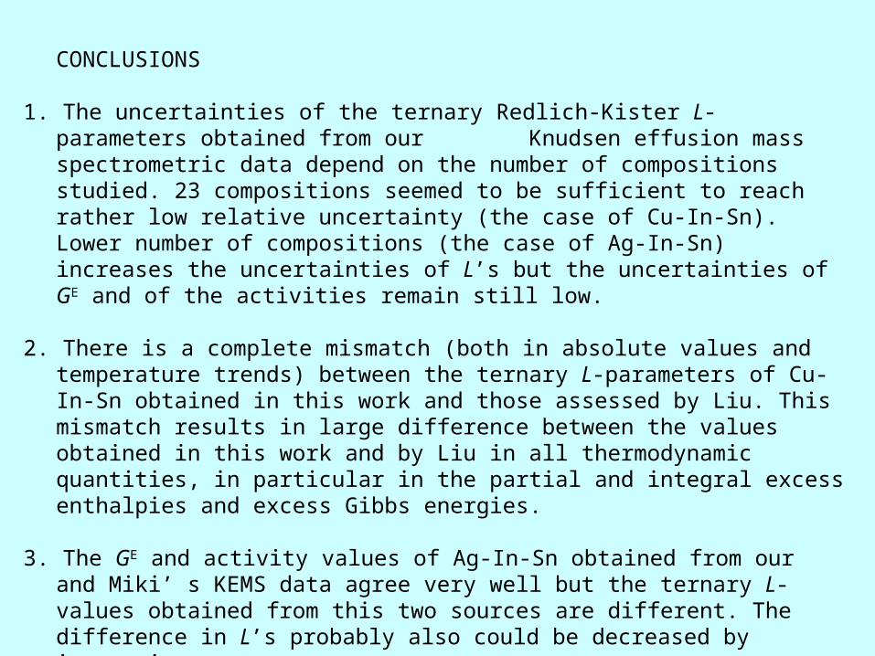
CONCLUSIONS
1. The uncertainties of the ternary Redlich-Kister L-parameters obtained from our Knudsen effusion mass spectrometric data depend on the number of compositions studied. 23 compositions seemed to be sufficient to reach rather low relative uncertainty (the case of Cu-In-Sn). Lower number of compositions (the case of Ag-In-Sn) increases the uncertainties of L’s but the uncertainties of GE and of the activities remain still low.
2. There is a complete mismatch (both in absolute values and temperature trends) between the ternary L-parameters of Cu-In-Sn obtained in this work and those assessed by Liu. This mismatch results in large difference between the values obtained in this work and by Liu in all thermodynamic quantities, in particular in the partial and integral excess enthalpies and excess Gibbs energies.
3. The GE and activity values of Ag-In-Sn obtained from our and Miki’ s KEMS data agree very well but the ternary L-values obtained from this two sources are different. The difference in L’s probably also could be decreased by increasing
the compositions studied.
4. Any ion pair variation (e.g. Ag+/Sn+ or Ag +/In+ in Ag-In-Sn) in the mass spectrum can be chosen in principle for obtaining the thermodynamic properties. The different choices must provide the same values in case of good consistency.

Many thanks to the COST 531 leadership for the support of my STSMs.
ACKNOWLEDGEMENTS
Thank You for Your attention!