Determination of Stress from Faults - · PDF fileChapter 11 Determination of Stress from...
32
Chapter 11 Determination of Stress from Faults Structural geologists observe deformations of rocks. However, they infer or constrain (paleo)stresses from faults. It is important to know not only the deformation but also the state of stress when the deformation occurs for the understanding of the mechanics of tectonics. In this chapter we study the methods for (paleo)stress analysis. The methods are useful to understand the present state of stress when they are applied to seismologi- cal data. In addition, the (paleo)stress field is important to understand the migration of fluids, including hydrocarbons and thermal water. Theories based on the Wallace-Bott hypothesis are introduced in the first half of this chapter. The sections after Section 11.6 introduce other theories on the relationship between faulting, stress, and deformation. 11.1 Mesoscale faults We observe fault on various scales at outcrops. Mesoscale faults are minor faults with displacements that can be grasped at one outcrop (Fig. 11.1), i.e., their displacements range from a few millimeters to several meters. The slip orientation of a fault is recognized by the scratches or grooves produced by fault movement on a fault surface. They are called fault striations or simply striae (Fig. 11.2). Offset of pre-faulting features such as strata tells the sense of shear (Fig. 11.1). Mesoscale faults can be reactivated. Those faults have two or a few sets of striae with different orientations. For the overlapping striae, the sense of shear can be identified for each set by asymmetrical minor structures along the striae [181]. It is possible to determine the relative chronology of the sets by their overlap- ping relationship. Consequently, one can recognize not only the orientation of a fault surface but the sense of shear and slip direction for each mesoscale fault. These are referred to as fault-slip data. For the following reasons, those faults are more often used than large-scale faults to investigate the stresses responsible for the movement of the faults. Firstly, the much greater number density of those faults than that of large-scale faults allows us to infer a stress field with a higher spatial resolution. Secondly, most large faults have a complicated history as they are sometimes reactivated and a large amount of work is needed to understand that history. Minor faults can be reactivated, but their history is believed to be simple. Repeated reactivation of a fault increases its total displacement, 271
Transcript of Determination of Stress from Faults - · PDF fileChapter 11 Determination of Stress from...

Chapter 11
Determination of Stress from Faults
Structural geologists observe deformations of rocks. However, they infer or constrain(paleo)stresses from faults. It is important to know not only the deformation but also thestate of stress when the deformation occurs for the understanding of the mechanics oftectonics. In this chapter we study the methods for (paleo)stress analysis. The methodsare useful to understand the present state of stress when they are applied to seismologi-cal data. In addition, the (paleo)stress field is important to understand the migration offluids, including hydrocarbons and thermal water. Theories based on the Wallace-Botthypothesis are introduced in the first half of this chapter. The sections after Section 11.6introduce other theories on the relationship between faulting, stress, and deformation.
11.1 Mesoscale faults
We observe fault on various scales at outcrops. Mesoscale faults are minor faults with displacementsthat can be grasped at one outcrop (Fig. 11.1), i.e., their displacements range from a few millimetersto several meters. The slip orientation of a fault is recognized by the scratches or grooves producedby fault movement on a fault surface. They are called fault striations or simply striae (Fig. 11.2).Offset of pre-faulting features such as strata tells the sense of shear (Fig. 11.1). Mesoscale faultscan be reactivated. Those faults have two or a few sets of striae with different orientations. For theoverlapping striae, the sense of shear can be identified for each set by asymmetrical minor structuresalong the striae [181]. It is possible to determine the relative chronology of the sets by their overlap-ping relationship. Consequently, one can recognize not only the orientation of a fault surface but thesense of shear and slip direction for each mesoscale fault. These are referred to as fault-slip data.
For the following reasons, those faults are more often used than large-scale faults to investigatethe stresses responsible for the movement of the faults. Firstly, the much greater number densityof those faults than that of large-scale faults allows us to infer a stress field with a higher spatialresolution. Secondly, most large faults have a complicated history as they are sometimes reactivatedand a large amount of work is needed to understand that history. Minor faults can be reactivated, buttheir history is believed to be simple. Repeated reactivation of a fault increases its total displacement,
271

272 CHAPTER 11. DETERMINATION OF STRESS FROM FAULTS
Figure 11.1: Mesoscale faults (arrows) in Pliocene forearc sediments, the Miyazaki Group, northernRyukyu arc, Japan [266]. The sediments and the faults are truncated by the angular unconformity(dotted line) on which Quaternary gravel layers lie, indicating that the faulting is older than theformation of the unconformity.
but mesoscale faults have small displacements. Thirdly, the deformation of a rock mass caused bya mesoscale fault within the mass can be treated as an infinitesimal deformation if the rock mass isvery large (§2.7).
The techniques introduced in this chapter utilize fault-slip data obtained from outcrops and ori-ented borehole cores to constrain (paleo)stresses. If those faults were generated by the present stressfield, the stress that they indicate is the present stress. The same techniques can be applied to seis-mological data to infer the present stress.
Several methods have been proposed to estimate the state of stress from faults. Among them,the most popular one is Anderson’s theory of faulting [4]. The theory is still used, as it is verysimple. However, one can trace modern methods back to the papers of the 1950s by Wallace andBott [20, 252]. Bott [20] explained the abundance of oblique slip faults, which were incompatiblewith Anderson’s theory (§6.3). McKenzie utilized Bott’s principle to infer the state of stress atan earthquake source [137]. The principle was used to formulate a mathematical inverse methodby Carey and Brunier [35] and by Angelier [6] in the 1970s to infer paleostresses from geological

11.2. WALLACE-BOTT HYPOTHESIS 273
Figure 11.2: Fault striations on a fault surface in Early Miocene strata, the Atsumi Formation, North-east Japan. There are comet-like structures heading right. They were produced by the drag of hardparticles between fault surfaces. These asymmetric structures indicate that this fault is dextral insense, i.e., the block on this side of the fault moved left.
faults. The inverse method was applied to many areas in the world. Since the mid 1990s, theoreticalinvestigations have been carried out on the numerical techniques to separate stresses from fault datathat record plural stresses [60, 161, 209, 264].
11.2 Wallace-Bott hypothesis
11.2.1 Basic equations
Modern methods for determining (paleo)stresses are based on the Wallace-Bott hypothesis [20, 252],stating that the shear traction applied on a given fault plane causes a slip in the direction and orien-tation of that shear traction, irrespective of the faults created in an intact rock or along a pre-existingfracture.
The traction vector at the fault plane whose unit normal is n is given by the equation
t(n) = r · n. (11.1)
From Eqs. (3.16) and (3.17), the normal and tangential components of this vector are the normaland shear traction vectors
σN = N · r · n = n[n · (r · n)
](11.2)
σS = (I − N) · r · n = r · n − n[n · (r · n)
]. (11.3)
274 CHAPTER 11. DETERMINATION OF STRESS FROM FAULTS
Faulting occurs to release the shear stress so the slip direction is indicated by the unit vector −σS/|σS|instead of σS.
The slip direction of a given fault has a linear relationship with the stress tensor r. To seethis, let us rewrite Eq. (11.3) as σS = f (r, n). Then the linearity is represented by the equationf (a1r(1) + a2r(2), n) = a1f (r(1), n) + a2f (r(2), n), where σ
(1)S and σ
(2)S are stress tensors and a1
and a2 are arbitrary scalar variables. Equation (11.3) is rewritten for these tensors as
σ(1)S = (I − N) · r(1) · n,
σ(2)S = (I − N) · r(2) · n,
so that we have
a1σ(1)S + a2σ
(2)S = a1(I − N) · r(1) · n + a2(I − N) · r(2) · n
= σS = (I − N) · [a1r(1) + a2r(2)] · n.Consequently, the slip direction predicted by the Wallace-Bott hypothesis has a linear relationshipwith stress tensors.
11.2.2 Graphical expressions of slip directions
The slip direction predicted by the Wallace-Bott hypothesis for a given fault and a stress is shown byMeans’ graphical method1 [142]. A tangent-lineation diagram is a graphical expression of fault-slipdata and is convenient for theoretical considerations.
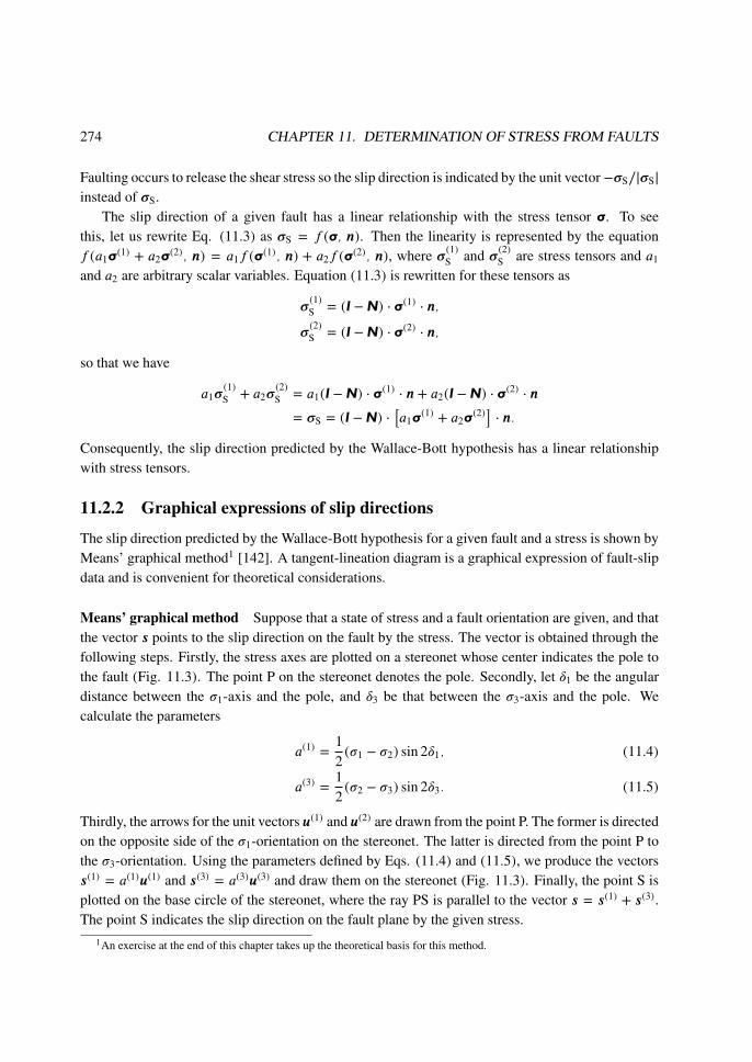
Means’ graphical method Suppose that a state of stress and a fault orientation are given, and thatthe vector s points to the slip direction on the fault by the stress. The vector is obtained through thefollowing steps. Firstly, the stress axes are plotted on a stereonet whose center indicates the pole tothe fault (Fig. 11.3). The point P on the stereonet denotes the pole. Secondly, let δ1 be the angulardistance between the σ1-axis and the pole, and δ3 be that between the σ3-axis and the pole. Wecalculate the parameters
a(1) =12
(σ1 − σ2) sin 2δ1, (11.4)
a(3) =12
(σ2 − σ3) sin 2δ3. (11.5)
Thirdly, the arrows for the unit vectors u(1) and u(2) are drawn from the point P. The former is directedon the opposite side of the σ1-orientation on the stereonet. The latter is directed from the point P tothe σ3-orientation. Using the parameters defined by Eqs. (11.4) and (11.5), we produce the vectorss(1) = a(1)u(1) and s(3) = a(3)u(3) and draw them on the stereonet (Fig. 11.3). Finally, the point S isplotted on the base circle of the stereonet, where the ray PS is parallel to the vector s = s(1) + s(3).The point S indicates the slip direction on the fault plane by the given stress.
1An exercise at the end of this chapter takes up the theoretical basis for this method.
11.2. WALLACE-BOTT HYPOTHESIS 275
Figure 11.3: Graphical method to determine the slip direction of a fault whose pole is plotted at thecenter of a stereonet.
Equations (11.4) and (11.5) demonstrate that the slip direction depends not only on the orienta-tion of stress axes but also on the ratio
R =σ1 − σ2
σ2 − σ3. (11.6)
This is related to the stress ratio as R = Φ/(1 −Φ), i.e., the slip direction depends on Φ. If the ratiois zero, the ray PS0 indicates the slip direction. The ray PS1 indicates the slip direction for the caseof Φ = 1. It should be stressed that Φ influences the slip direction as much as the principal stressorientations do.
The graphical method demonstrates that slip directions are directed away from the σ1-axis andtoward the σ3-axis. If the fault in Fig. 11.3 is nearly perpendicular to the σ2-axis, the angles δ1 andδ3 are approximately equal to 90◦. Therefore, a(1) ≈ a(3) ≈ 0, though their signs depend on the tinydifference of the angles from 90◦. This further indicates that the slip direction, s, is swerved aroundthe σ2-axis.
Tangent-lineation diagram A tangent-lineation diagram is a convenient graphical method to il-lustrate the slip directions.
The plane containing the slip vector and the pole to the fault plane is called the M-plane of thefault. The plane perpendicular to the M- and fault planes is know as an auxiliary plane (Fig. 11.4(a)).A fault-slip datum is expressed in the diagram by an arrow plotted on a lower-hemisphere stereonet(Fig. 11.4(b)). The position of the arrow in the stereonet indicates the pole to the fault plane. Thearrow is drawn parallel to the M-plane, and is pointing at the slip direction of the footwall.
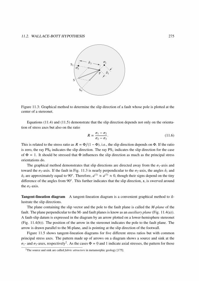
Figure 11.5 shows tangent-lineation diagrams for five different stress ratios but with commonprincipal stress axes. The pattern made up of arrows on a diagram shows a source and sink at theσ1- and σ3-axes, respectively2. As the cases Φ = 0 and 1 indicate axial stresses, the pattern for those
2The source and sink are called fabric attractors in metamorphic geology [175].

276 CHAPTER 11. DETERMINATION OF STRESS FROM FAULTS
Figure 11.4: (a) Schematic picture showing the orientation of a reverse fault plane and the directionof fault movement (bold arrows). The line OQ indicates the orientation of striae, and the point Pis the pole to the fault plane. The arrow attached to the point P indicates the slip direction of thefootwall block. The plane containing the triangle OPQ is called the M-plane for the fault. The planeperpendicular to the fault plane and M-plane is called the auxiliary plane. (b) Lower-hemispherestereonet showing the three planes and the slip direction of the footwall that is depicted by the arrowattached to the point P. The line OB is the intersection of the fault and auxiliary plane.
cases shows axial symmetry about the σ1- and σ3-axis, respectively. The pattern exhibits orthorhom-bic symmetry for triaxial stresses, and a saddle point appears at the σ2-orientation. Tangent-lineationdiagram for a set of natural fault-slip data is shown in Fig. 11.6.
11.2.3 Indeterminacy of stress from faults
Fault-slip data constrain the state of stress that was responsible for the faults. However, not all thestress components are determined. The Wallace-Bott hypothesis indicates that slip directions arenot affected by pore fluid pressure, although it controls the strength of faults. The effective stressis given by the equation r′ = r − pI. Thanks to the linearity, the slip direction due to r′ is thelinear combination of those by r and −pI. However, the latter is an isotropic stress and causes noshear traction. Therefore, the pore fluid pressure does not affect the slip direction of a fault. This isconvenient for paleostress analysis, because it is difficult to know the pore fluid pressure on a faultsurface when the fault moved.
It is also difficult to estimate the depth of burial of a fault when it was activated. However, thedepth has little affect on the slip direction. Crustal stress is limited by the brittle strength (§6.7),and faulting occurs when stress is brought to the limit. Equation (6.21) indicates that the limitingstress is proportional to the depth z. Let r0 be an arbitrary stress tensor. Since the slip directionsdue to stresses r0 and r = qr0 are the same, the slip directions are independent from the depthof burial. However, this is valid only as an approximation, because stress states inferred by in-situmeasurements more or less deviate from the proportionality.
11.2. WALLACE-BOTT HYPOTHESIS 277
Figure 11.5: Tangent-lineation diagrams showing the slip directions of faults by stresses with thesame principal orientations but different stress ratios. The principal orientations are shown in thelower right box. Open circles in the stereonets indicate the poles to the fault plane.
The slip directions predicted by the Wallace-Bott hypothesis for the stresses r and
r = qr0 − pI (11.7)
are the same for a given fault, whether or not p and q are interpreted as pore pressure and depth.When the state of stress is illustrated by Mohr circles, p and q indicate the position of the circles onthe abscissa and the size of the circles, respectively. The stresses that have common principal orien-tations and similar stress ellipsoids have similar Mohr circles, and result in identical slip directions.The tensor that represents those stresses is termed reduced stress tensor.
Due to the insensibility of the slip direction to these parameters, fault-slip it is not enough toconstrain the mean and differential stresses. However, this is convenient for paleostress analysis,because we do not need to worry about the depth and pore fluid pressure when each fault wasactivated3. These quantities are difficult to estimate.
It is convenient to assume a special form for r0 to consider slip directions. For example, we can
3Researchers have attempted to determine all the stress components from fault-slip data with assumption such as the brittlestrength of rocks [8].

278 CHAPTER 11. DETERMINATION OF STRESS FROM FAULTS
Figure 11.6: Natural fault-slip data obtained from the Otadai Formation, mid Quaternary forearcbasin deposit in central Japan [151]. The left panel is the tangent-lineation diagram showing thedata. The right panel is the lower-hemisphere stereonet in which the orientations of fault planesare indicated by great circles. Open circles on the great circles designate the orientation of faultstriations, and arrows attached to the open circles show the sense of shear. If an arrow is attached,it indicates the slip direction of the hanging wall. If two arrows are attached to an open circle, thearrows depict the sinistral or dextral sense of shear.
express any stress tensor by combining Eq. (11.7) and
r0 = RT ·⎛⎝1 0 0
0 Φ 00 0 0
⎞⎠ · R, (11.8)
where R indicates the principal stress orientations and Φ = (σ2 − σ3)/(σ1 − σ3) is the stress ratio.The tensor between RT and R in Eq. (11.8) is a reduced stress tensor, but the definition of a reducedstress tensor is not unique [7]. Different shapes of reduced tensor is introduced in Section 11.5 andin Appendix B.
The tensor r0 in the shape of Eq. (11.8) is enough to calculate the slip directions of faults. Theorthogonal tensor R has three degrees of freedom corresponding to the three Euler angles (Fig. C.5).The reduced stress tensor has one degree of freedom. Therefore, r0 has four degrees of freedom.However, the stress tensor has six degrees of freedom. The difference corresponds to p and q in Eq.(11.7). The tensor r0 represents the principal orientations and stress ratio. In this chapter, the term“a state of stress” is used to denote the stresses with a common r0.
A fault-slip datum does not tightly constrain the principal stress orientations. It should be notedthat different stresses can result in a fault-slip datum. The admissible orientations for the datum areillustrated in Fig. 11.7. The possible principal σ1 orientation reduces by a decrease of stress ratio,which in turn expands the possible σ3 orientation. It is known that both the σ1- and σ3-axes exist onone side of the plane AOC [122]. Namely, if the domain OBC in Fig. 11.7 has the σ1-axis, then the

11.2. WALLACE-BOTT HYPOTHESIS 279
Figure 11.7: Stereogram (upper hemisphere) showing the principal stress orientations compatiblewith a fault-slip datum. The upper block is assumed to move rightwards on the plane ABCD. P-and T-axes are contained in the plane AOC and make angles of 45◦ with O. They approximate
the σ1- and σ3-orientations if the Coulomb-Navier criterion holds for this fault. The Wallace-Botthypothesis predicts the σ1-axis in the region OBCD for this fault. The σ3-axis is oriented in theregion OBAD. The σ1-orientation is constrained more tightly for a prescribed stress ratio. Dottedlines with decimal fractions show the rightward limit of the permissible region for the σ1-axis, wherethe fractions indicate stress ratios. The lines are obtained from Eq. D.45.
σ3-axis must exist in the domain OAB.
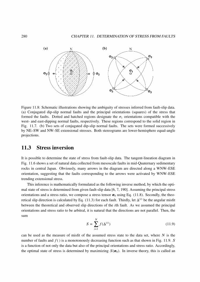
For example, if there are conjugated N–S trending normal faults formed by the E–W extensionalstress with Φ = 0.5 (Fig. 11.8(a)), the stress compatible with the fault-slip data is not unique.Stresses with a wide variation of principal orientations and stress ratios are compatible with the data.However, if there are varieties of fault attitudes and of slip directions, the admissible stresses areconstrained as the overlapping region of the dotted and hatched regions in Fig. 11.8(a).
Figure 11.8(b) shows the case of two conjugated normal faults with different ages and differentextensional orientations. If we do not know the difference and we regard them as the results of thesame state of stress, the vertical axial compression is a possible stress compatible with the data, i.e.,it is not possible to distinguish from the data which scenario is correct, the two-phase or the single-phase stress history. The set of stress states compatible with given data set are said to be associatedstresses [264]. Other lines of evidence are needed to determine the correct stresses.
280 CHAPTER 11. DETERMINATION OF STRESS FROM FAULTS
Figure 11.8: Schematic illustrations showing the ambiguity of stresses inferred from fault-slip data.(a) Conjugated dip-slip normal faults and the principal orientations (squares) of the stress thatformed the faults. Dotted and hatched regions designate the σ1 orientations compatible with thewest- and east-dipping normal faults, respectively. These regions correspond to the solid region inFig. 11.7. (b) Two sets of conjugated dip-slip normal faults. The sets were formed successivelyby NE–SW and NW–SE extensional stresses. Both stereograms are lower-hemisphere equal-angleprojections.
11.3 Stress inversion
It is possible to determine the state of stress from fault-slip data. The tangent-lineation diagram inFig. 11.6 shows a set of natural data collected from mesoscale faults in mid-Quaternary sedimentaryrocks in central Japan. Obviously, many arrows in the diagram are directed along a WNW–ESEorientation, suggesting that the faults corresponding to the arrows were activated by WNW–ESEtrending extensional stress.
This inference is mathematically formulated as the following inverse method, by which the opti-mal state of stress is determined from given fault-slip data [6, 7, 190]. Assuming the principal stressorientations and a stress ratio, we compose a stress tensor r0 using Eq. (11.8). Secondly, the theo-retical slip direction is calculated by Eq. (11.3) for each fault. Thirdly, let Δ(i) be the angular misfitbetween the theoretical and observed slip directions of the ith fault. As we assumed the principalorientations and stress ratio to be arbitral, it is natural that the directions are not parallel. Then, thesum
S =N∑i=1
f (Δ(i)) (11.9)
can be used as the measure of misfit of the assumed stress state to the data set, where N is thenumber of faults and f ( ) is a monotonously decreasing function such as that shown in Fig. 11.9. Sis a function of not only the data but also of the principal orientations and stress ratio. Accordingly,the optimal state of stress is determined by maximizing S(r0). In inverse theory, this is called an

11.3. STRESS INVERSION 281
Figure 11.9: Graph of a monotonously decreasing function f (Δ) used in stress inversion.
object function.This method is referred to as stress inversion4. Contrasting with the recent numerical techniques
that are introduced in the next section, this is sometimes called the classical inverse method. Thestress inversion is a non-linear inverse method, because the slip direction is denoted by the unitvector −σS/|σS|. The non-linearity comes from this division [150].
The optimal stress determined by the stress inversion has uncertainty resulting from the indepen-dence of the slip direction from p and q in Eq. (11.7). The absolute values of stress componentsare not known. Instead, the tensor defined by Eq. (11.8) is determined, i.e., the optimal principalorientations and the optimal stress ratio are obtained by the inverse method.
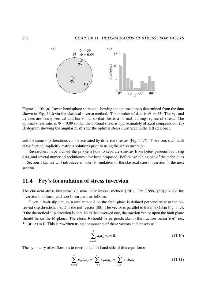
Figure 11.10 shows the optimal stress determined through the stress inversion for the natural datain Fig. 11.6. The result is a WNW–ESE trending extensional stress, which coincides with the stressroughly inferred by eye from the tangent-lineation diagram of the data.
However, the optimal solution is not satisfactory as the histogram of angular misfits is definitelybimodal. About two-fifths of the faults have misfits greater than 60◦. The optimal stress cannotexplain the observed slip directions of those faults, indicating that the fault-slip data are heteroge-neous. Fault-slip data is called heterogeneous if plural stress states were responsible for the faults.Consequently, the forearc region in central Japan experienced a polyphase stress history since theOtadai Formation, from which the data were obtained, deposited in the mid Quaternary [151].
Given heterogeneous fault-slip data the object function S(r0) has maxima, and the optimal so-lution might be a meaningless solution [265]. Thus, we have to input homogeneous fault-slip datafor the calculation. For this purpose, researchers try to sort faults at outcrops by their apparent ages.
There are several criteria [10, 39, 250]. The principal guides for distinguishing the different faultsets are (1) consideration of stratigraphy or of the age of the rocks affected by a certain deformation,(2) characterization of the synsedimentary faults such as fault drag, (3) cross-cutting relationships,(4) superimposed striae on the same fault plane and (5) association of mineral veins. Unfortunately,these criteria are not always available in the field, especially in young geologic units such as the mid-Quaternary Otadai Formation. In addition, the resemblance of the orientation of fault planes and slipdirections is sometimes employed for fault sorting. However, many faults with the same orientations
4See [9] for further reading.
282 CHAPTER 11. DETERMINATION OF STRESS FROM FAULTS
Figure 11.10: (a) Lower-hemisphere stereonet showing the optimal stress determined from the datashown in Fig. 11.6 via the classical inverse method. The number of data is N = 53. The σ1- andσ3-axes are nearly vertical and horizontal so that this is a normal faulting regime of stress. Theoptimal stress ratio is Φ = 0.09 so that the optimal stress is approximately of axial compression. (b)Histogram showing the angular misfits for the optimal stress illustrated in the left stereonet.
and the same slip directions can be activated by different stresses (Fig. 11.7). Therefore, such faultclassification implicitly restricts solutions prior to using the stress inversion.
Researchers have tackled the problem how to separate stresses from heterogeneous fault slipdata, and several numerical techniques have been proposed. Before explaining one of the techniquesin Section 11.5, we will introduce an other formulation of the classical stress inversion in the nextsection.
11.4 Fry’s formulation of stress inversion
The classical stress inversion is a non-linear inverse method [150]. Fry (1999) [60] divided theinversion into linear and non-linear parts as follows.
Given a fault-slip datum, a unit vector b on the fault plane is defined perpendicular to the ob-served slip direction, i.e., b is the null vector [80]. The vector is parallel to the line OB in Fig. 11.4.If the theoretical slip direction is parallel to the observed one, the traction vector upon the fault planeshould lie on the M-plane. Therefore, b should be perpendicular to the traction vector t(n), i.e.,b · (r · n) = 0. This is rewritten using components of these vectors and tensors as
3∑i,j=1
biσijnj = 0. (11.10)
The symmetry of r allows us to rewrite the left-hand side of this equation as
3∑i,j=1
σijbinj =3∑
i,j=1
σjibinj =3∑
i,j=1
σijbjni. (11.11)
11.4. FRY’S FORMULATION OF STRESS INVERSION 283
In the last transformation, the dummy indices i and j are exchanged. Consequently, Eq. (11.10) isrewritten as
3∑i,j=1
bjσijni = 0. (11.12)
Adding both sides of Eqs. (11.10) and (11.12) gives5
3∑i,j=1
σijfij = 0, (11.13)
where
fij = binj + bjni.
Note that n and b are observable quantities but r is unknown. Accordingly, we can compose thetensor fij from the fault-slip datum. In addition, fij has six degrees of freedom, because of thesymmetry fij = fji. Therefore, Eq. (11.13) is further rewritten as the scalar product
s · f = 0, (11.14)
where s = (σ11, σ12, σ13, σ22, σ23, σ33)T and f = (f11, f12, f13, f22, f23, f33)T. The componentsof these vectors are independent components of the tensors σij and fij.
Equation (11.14) indicates that the vectors s and f meet at right-angles in six-dimensional spaceif the assumed stress r fits the fault-slip datum. If |s · f | does not vanish, r is not appropriate for thedatum. Accordingly, we define the unit vector f = f/|f | so that the endpoint of the position vectorf is represented by a point on the six-dimensional unit sphere.
Let f (k) be the unit vector for the kth datum. If the stress is compatible with all the fault-slipdata, then the stress tensor must satisfy the equation
N∑k=1
s · f (k) = 0. (11.15)
This equation has the geometrical interpretation that the end points of the unit vectors, f(1), . . . ,
f(N)
, are on the great circle whose pole is parallel to the vector s. The scalar product s · f becomesnegative in sign if the angle between the two vectors is greater than 90◦. Therefore, the stressinversion can be reformulated as the least-squares method to minimize the quantity
N∑k=1
[s · f (k)]2
.
5Comparing the following equation with Eqs. (2.49) and (2.54) in Section 2.7, it is seen that Eq. (11.13) indicates thatthe work done by the shear traction in the orientation perpendicular to the observed slip direction is nil.

284 CHAPTER 11. DETERMINATION OF STRESS FROM FAULTS
This is equivalent withto
N∑k=1
[ 6∑i=1
sif(k)i
][ 6∑j=1
sjf(k)j
]=
N∑k=1
6∑i,j=1
sif(k)i f
(k)j sj =
6∑i,j=1
si
[N∑k=1
f(k)i f
(k)j
]sj = s · g · s,
where
g =
(N∑k=1
f(k)i f
(k)j
)is a six-dimensional, second-order, symmetric tensor, and is composed from given fault-slip data.
The optimal stress determined by the stress inversion has uncertainty resulting from the indepen-dence of the slip direction from p and q in Eq. (11.7). The absolute values of the stress componentsare not known. Accordingly, the uncertainty allows us to assume s to be a unit vector.
The least-squares method that we should solve is to search the optimal vector s that minimizesthe quadratic form s · g · s with the constraint s · s = 1. The constraint designate that the end pointof the vector is on the six-dimensional unit sphere. This extreme value problem is solved throughLagrange’s method of the undetermined multiplier, i.e., we seek the extremal of the function,
L = s · g · s − λ(s · s − 1) = 2s · (g − λI) · s − λ,where λ is the Lagrange multiplier. Since the tensor (g−λI) is symmetric, the formula in Eq. (C.61)applies to this tensor, and we obtain
∂L∂s
= 2(g · s − λs) = 0.
Consequently, we obtain the characteristic equation,
g · s = λs. (11.16)
A symmetric tensor has real eigenvalues. Therefore, all the roots of this equation are real. We areseeking the eigenvector s that minimizes L. Noticing s · s = 1, we obtain s · g · s = s · λs = λ fromEq. (11.16). The left-hand side of this equation equals L so that the minimum absolute eigenvaluecorresponds to the minimum L, and the corresponding eigenvector gives the optimal stress [209].
It was shown that the optimal vector s is parallel to the pole to the great circle along which the
endpoints of the data vectors f(1), . . . , f
(N)are aligned. Fitting of a great circle to the data vectors
is a eigenproblem to solve Eq. (11.16). This is a linear inverse problem.Once a great circle is fitted, we have two poles for that circle. If one of the poles is represented by
s, the other is −s. These vectors correspond to the stresses r and −r. Therefore, we have to chooseone of them. The slip directions corresponding to the stresses are given by −σS = ±(N − I) · r · n(Eq. (11.3)). That is, the stresses causes the opposite sense of movement for entire faults so thatwe can choose one of the stresses corresponding to the correct sense of movement. The choice ofthe correct pole is a non-linear operation. The stress inversion is, therefore, divided into linear andnon-linear parts6.
6See Appendix B and [203, 269].
11.5. MULTIPLE INVERSE METHOD 285
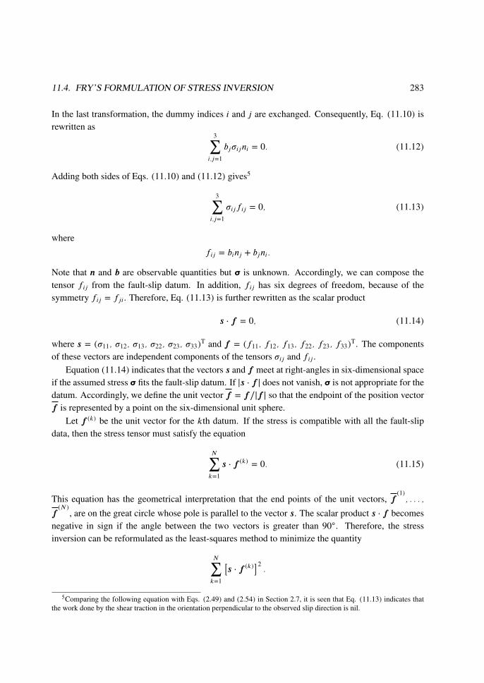
Figure 11.11: Schematic illustrations showing the principle of the multiple inverse method. (a) Datapoints are aligned on two great circles (dotted lines) on the six-dimensional unit sphere. (b) Whitearcs showing parts of the great circles that are fitted to k-element subsets of the data points, where kgenerally equals 5. (c) The poles of the great circles are plotted to exhibit the optimal stress for thesubsets. The poles make clusters at the poles for the great circles indicated by the dotted lines in (a).
11.5 Multiple inverse method
The purpose of this section is to explain the multiple inverse method, a numerical technique used forseparating stresses from heterogeneous fault-slip data [264].
11.5.1 Principle
It was shown in the previous section that the stress inversion is compared to fitting a great circle todata points on the six-dimensional unit sphere, and that one of the poles of the great circle representsthe optimal stress. Therefore, heterogeneous fault-slip data are represented by data points that arealigned on plural great circles on the unit sphere. Suppose that a set of observed faults is a mixtureof two assemblages that were activated by two different stresses. Then, the fault-slip data are repre-sented by two great circles on the unit sphere (Fig. 11.11(a)). Consequently, it is the problem howto identify the great circles. The basic idea of the method is that the generalized Hough transformis applicable to this problem. The transform is a technique of artificial intelligence to detect objectswith arbitrary shapes and orientations [31]. The objects in our problem are stress ellipsoids withdifferent shapes and different orientations.
The method firstly constructs k-element subsets from the entire fault-slip data. Given N faults,we have NCk subsets, where
NCk =N!
k!(N − k)!
is the binomial coefficient. Secondly, great circles are fitted to the subsets7. Thirdly, the poles of thegreat circles that represent the optimal stresses for the subsets are plotted on the unit sphere. There
7It was shown that the resolution of this method is greatly improved by choosing a particular kind of subsets [168].
286 CHAPTER 11. DETERMINATION OF STRESS FROM FAULTS
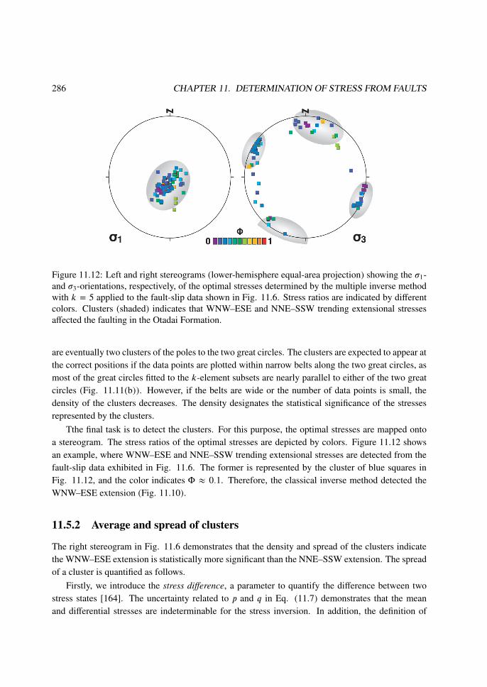
Figure 11.12: Left and right stereograms (lower-hemisphere equal-area projection) showing the σ1-and σ3-orientations, respectively, of the optimal stresses determined by the multiple inverse methodwith k = 5 applied to the fault-slip data shown in Fig. 11.6. Stress ratios are indicated by differentcolors. Clusters (shaded) indicates that WNW–ESE and NNE–SSW trending extensional stressesaffected the faulting in the Otadai Formation.
are eventually two clusters of the poles to the two great circles. The clusters are expected to appear atthe correct positions if the data points are plotted within narrow belts along the two great circles, asmost of the great circles fitted to the k-element subsets are nearly parallel to either of the two greatcircles (Fig. 11.11(b)). However, if the belts are wide or the number of data points is small, thedensity of the clusters decreases. The density designates the statistical significance of the stressesrepresented by the clusters.
Tthe final task is to detect the clusters. For this purpose, the optimal stresses are mapped ontoa stereogram. The stress ratios of the optimal stresses are depicted by colors. Figure 11.12 showsan example, where WNW–ESE and NNE–SSW trending extensional stresses are detected from thefault-slip data exhibited in Fig. 11.6. The former is represented by the cluster of blue squares inFig. 11.12, and the color indicates Φ ≈ 0.1. Therefore, the classical inverse method detected theWNW–ESE extension (Fig. 11.10).
11.5.2 Average and spread of clusters
The right stereogram in Fig. 11.6 demonstrates that the density and spread of the clusters indicatethe WNW–ESE extension is statistically more significant than the NNE–SSW extension. The spreadof a cluster is quantified as follows.
Firstly, we introduce the stress difference, a parameter to quantify the difference between twostress states [164]. The uncertainty related to p and q in Eq. (11.7) demonstrates that the meanand differential stresses are indeterminable for the stress inversion. In addition, the definition of
11.5. MULTIPLE INVERSE METHOD 287
a reduced stress tensor is not unique. Accordingly, we define the reduced stress tensor r so as tosatisfy the two conditions
trace r = σ11 + σ22 + σ33 = 0 (11.17)
and the octahedral shear stress of unity. Equation (11.17) indicates that r is a deviatoric tensor sothat the second basic invariant of this tensor is given by Eq. (4.13). Following Eq. (4.17), we havethe second condition as
13
(σ2
11 + σ222 + σ
233 + 2σ2
12 + 2σ223 + 2σ2
31
)= 1. (11.18)
Using the reduced stress, we have the stress tensor R · r · RT for the stress tensor inversion.Secondly, given two reduced stress tensors, r(1) and r(2), the difference between the stress states
represented by the tensors is defined by the octahedral shear stress of the tensor D = r(1) − r(2).Namely, the difference is given by
D =13
√(Δ11 − Δ22)2 + (Δ22 − Δ33)2 + (Δ33 − Δ11)2 + 6 (Δ12)2 + 6 (Δ23)2 + 6 (Δ31)2. (11.19)
Orife and Lisle [164] term this parameter “stress difference”, and demonstrate that D is in the rangebetween 0 and 2 for any combination of reduced stress tensors provided that they satisfy the con-ditions indicated by Eqs. (11.17) and (11.18). The similarlity between two reduced stress tensorsis indicated by (2 − D). If D = 0, the two stress states result in the same slip directions whateverthe orientations of faults are. If D = 2, the two stress states cause faulting with the opposite slipdirections. The couple of stresses with D = 2 are called inverse stresses.
Finally, the spread of stress states is defined as follows. Given m reduced stress tensors, r(1), . . . ,
r(m), their average is defined by
〈r〉 = 1m
[r(1) + · · · + r(m)
]. (11.20)
The average principal orientations are obtained as the eigenvectors of this tensor, and the averagestress ratio is given by the equation
〈Φ〉 = 〈σ〉2 − 〈σ〉3
〈σ〉1 − 〈σ〉3,
where 〈σ〉i is the ith largest eigenvalue of the tensor 〈r〉. The spread of the reduced stress tensorsaround the average is defined by the average stress difference
〈D〉 = 1m
[D(1) + · · · +D(m)] , (11.21)
whereD(i) is the stress difference between r(i) and the reduced stress tensor derived 〈r〉. The greaterthe scatter of the stress states the larger the average stress difference. Therefore, 〈D〉 is a measure ofthe spread of stress states8.
8he average of the values of 2 sin−1(D/2) is more useful than that of D values. See Appendix B.
288 CHAPTER 11. DETERMINATION OF STRESS FROM FAULTS
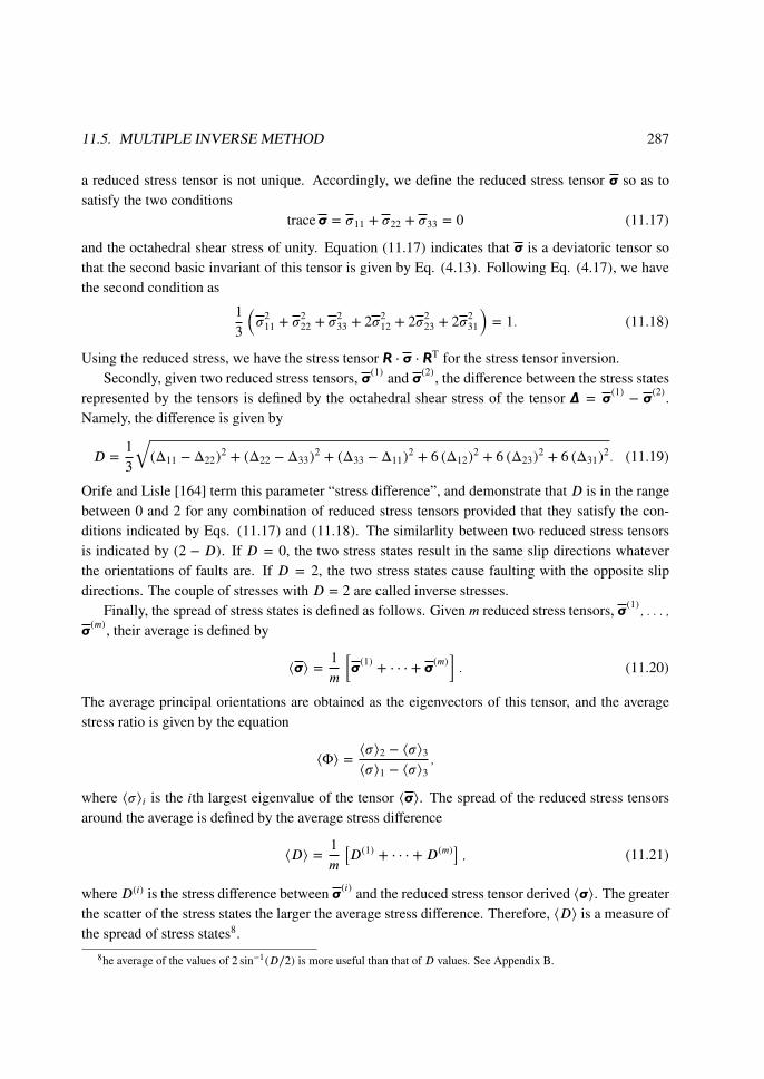
Figure 11.13: Mohr circles for a triaxial stress and the slope tanχ.
The multiple inverse method yields clusters of stress states, and the center and spread of a clusterare evaluated by Eqs. (11.20) and (11.21). The identification of those clusters can be computerizedusing the k-means algorithm [167], a technique of artificial intelligence [52], with the average andspread of the clusters.
It is difficult to apply stress inversion to fold belts as the timing of faulting relative to folding isdifficult to know. Therefore, it is sometimes assumed a-priori that a reverse faulting regime of stressaccompanied folding.
The bedding tilt test used in paleomagnetism can be applied to this problem using the multipleinverse method and the average and spread of clusters [270]. Paleomagnetists uses the statistic α95 toevaluate the spread of paleomagnetic vectors determined at various parts of a fold [32]. The larger thestatistic, the more the vectors are scattered. If rocks in the fold acquired the paleomagnetism beforefolding, untilting of the vectors makes α95 smaller. If, on the other hand, the rocks were magnetizedafter folding, the statistic becomes larger by the untilting. Therefore, the statistic works as an objectfunction to be minimized in the inverse problem to determine the optimal timing magnetizationrelative to folding.
Similarly, we are able to use 〈D〉 instead of α95 to be minimized in the inverse problem fordetermining the optimal timing of faulting relative to folding. This test procedure was applied tomesoscale faults in a Quaternary fold in central Japan and revealed that the majority of the faultswere activated by a strike-slip faulting regime of stress at the middle of folding [270].
11.6 Slip tendency
The Wallace-Bott hypothesis concerns the fact that any faults can be activated, unless the fault planeis one of the principal planes of stress. Shear stress on the plane vanishes so that those faults cannotmove. However, if fault planes have the same coefficient of friction, faults nearly parallel to theprincipal plane may be difficult to move compared to those oblique to the principal planes. Themagnitude of shear stress is depicted by the Mohr diagram (Figs. 4.6 and 11.13).
Slip tendency [157] is a yardstick for the mobility of fault surfaces under a given stress r. The
11.6. SLIP TENDENCY 289
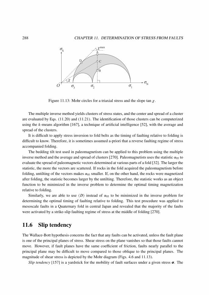
Figure 11.14: Stereonets showing slip tendency Ts for three stresses with the same principal orien-tations (open circles) but with different stress ratios, Φ = 0, 0.5 and 1.
frictional resistance of the fault with the unit normal n is μfσN = μf (n · r · n). A fault is thoughtto be preferable for r if the shear stress on the fault, σS = |(I − N) · r · n|, is much large comparedwith Fs, i.e., the slip tendency is defined as
Ts ≡∣∣∣∣ σS
μfσN
∣∣∣∣ =1μf
∣∣∣∣ (I − N) · r · nn · r · n
∣∣∣∣ .Ts is a function of n, r and μf . Given r and μf , Ts has the maximum Tmax
s for the fault orientations.
For simplicity, we assume that all faults have the same coefficient of friction to investigate therelationship of the mobility with fault orientations. Then, the angle χ shown in Fig. 11.13 is relatedto the slip tendency as tanχ = Ts. The points A, B and C have a common normal stress but differentshear stresses. The points A and B have maximum and minimum χs, respectively. It is obvious thatthe fault plane designated by point D has the maximum χ, because the line OD is tangent to the outerMohr circle. However, the Mohr diagram is not convenient to see how the slip tendency changeswith different orientations.
Therefore, the ratio Ts/Tmaxs is a convenient measure to consider the orientation-dependence of
the slip tendency. The variation of this ratio is shown by the gray scales in Fig. 11.14. The centralpanel in this figure illustrates the relationship between the slip tendency and fault orientations fortriaxial stresses. There are two dark spots in the stereogram, demonstrating that the fault surfacesparallel to the σ2-axis and making an acute angle with σ1-axis have a maximum slip tendency undertriaxial stresses. The two spots represent conjugate faults. The slip tendency has a orthorhombicsymmetry with respect to the principal planes of stress.
In contrast, the slip tendency for axial compression and axial tension has axial symmetry withrespect to the σ1- and σ3-axes, respectively (Fig. 11.14). The planes tangent to a cone whose axis isparallel to the symmetry axis of stress are referentially activated as faults [95].
In reality, every fault may have its own coefficient of friction, and pore pressure may be differentfor each faulting event. Accordingly, the slip tendency is not the only factor to indicate the mobility.However, Fig. 11.14 helps in considering fault activity under a specified state of stress.

290 CHAPTER 11. DETERMINATION OF STRESS FROM FAULTS
Figure 11.15: Strain of a rock mass by the activity of fault sets in the mass, where faults belongingto a set have similar fault orientations and slip directions. Rectangle ABCD indicates the initial topsurface of the mass. The z-axis is defined as being vertically downward. Although displacement isshown along two or several faults for each set, the parallel faults carry similar displacements. (a)The activity of a set of normal faults parallel to the y-axis and slip direction normal to the y-axis, themass suffers a plane strain on the xz-plane. The points B and C are transferred to B′ and C′ by thefaulting, resulting in an inclined top surface AB′C′D. (b) Two sets of faults making up conjugatednormal faults. If the total displacements of each set are equal to each other, the top surface remainshorizontal only to subside to the rectangle A′B′C′D′. The deformation of the mass is approximatedby a pure shear. (c) Four sets of faults leading to a three-dimensional coaxial deformation, i.e., thetop surface is kept horizontal.
11.7 Faulting controlled by strain
A rock mass encompassing faults deforms by the fault activity (Fig. 1.17). If there are a lot of faultswith much smaller displacements than the size of the mass, the deformation can be regarded as acontinuous plastic deformation.
Faulting obeying Anderson’s theory leads only to a plane strain (Exercise 11.1). However, strainsmay be generally three-dimensional. The faulting predicted by the Wallace-Bott hypothesis allowsthree-dimensional strains. When we used the hypothesis, stress was assumed to control faulting.However, stress is not observable. We observe the strain of a rock mass through faults, and thehypothesis transforms strain into stress. In contrast, what would happen if strain controls faulting?The present and next sections deal with this problem.
Natural faults often form groups with similar orientations and slip directions. Here, we sort faultsby the orientations and directions into sets of faults (Fig. 11.15). One region may have multiple setsof faults, which may or may not have been activated at the same time.
For simplicity, we assume that all faults belonging to a set have the same displacements and thatthey are uniformly distributed in the rock mass. Then, the deformation of the mass due to internalfault activity can be regarded as a uniform deformation. The deformation by a single set of faults

11.8. RECHES’ MODEL 291
equals an infinitesimal simple shear in the M-plane of the faults. The top surface ABCE in Fig.11.15(a) is transformed into the inclined rectangle AB′C′D by this simple shear unless the faultplanes are horizontal. Two sets of faults enable pure shears that keep the top surface horizontal (Fig.11.15(b)). If there are four sets of faults, coaxial deformations are possible (Fig. 11.15(c)).
Not only coaxial but also any three-dimensional deformations are possible if there are at leastfour fault sets [193]. Here, faulting is assumed not to accompany any volume change of the rockmass, so that we have |F| = 1, where F is the deformation gradient of the rock mass. F has nine in-dependent components in three dimensions. However, the volume conservation reduces the degreesof freedom of F to eight. One set has two degrees of freedom, the rake of slip direction on the faultplanes and the parameter q of the simple shear (Eq. (1.13)), if the orientations of fault planes aregiven. Therefore, four fault sets are sufficient to accommodate a general incompressive deformationin three dimensions.
If a three-dimensional deformation controls faulting, at least a few sets of faults should be acti-vated to accommodate the deformation. Fault systems comprised of four fault sets are often observedin the field and in clay cake experiments [131, 163, 193, 195].
11.8 Reches’ model
We now consider faulting controlled by a prescribed strain of a rock mass that includes the faults.Reches [193, 194] applied a classical theory of the plastic deformation of single crystals. The plasticdeformation is due to the movement of dislocations through the crystal lattice. The lattice structureallows a limited number of slip systems whose glide planes and slip directions are constrained.For example, a face-centered cubic lattice has 12 slip systems. Minimizing energy dissipation,Taylor (1938) linked the slippage on the planes with the macroscopic deformation of the crystalcontaining the slip systems [239]. Unlike single crystals, a rock mass has numberless planes offractures with various orientations that are capable of faulting. However, the following argumentreduces the possible number of fault sets to four.
It is assumed that there are numberless pre-existing fractures capable of accommodating an ap-plied three-dimensional coaxial strain, but that most preferable surfaces are activated. The rockmass is also assumed to be homogeneous and isotropic in the broad view so that the stress andstrain have the same principal orientations. Since the controlling factor is the coaxial strain that hasan orthorhombic symmetry about the principal planes of strain, the resultant faulting may have thesame symmetry, i.e., the four sets of faults the orientations of which are arranged symmetricallywith respect to the planes (Fig. 11.16(a)). Four sets are necessary and sufficient to accommodate theprescribed strain of the rock mass. To keep the symmetry, they carry the same magnitude of strain.Here, they are called orthorhombic fault sets.
Each fault set has many faults but the displacements are very small compared to the dimensionof the rock mass. In addition, faults belonging to a set are located with constant intervals. Therefore,the deformation of the mass is regarded as continuous and homogeneous. Let the unit vectors n(i) =

292 CHAPTER 11. DETERMINATION OF STRESS FROM FAULTS
Figure 11.16: (a) Orthorhombic fault sets arranged symmetrical with respect to the principal planesof stress. Equal-angle projection. The rectangular Cartesian coordinates O-123 are defined as beingparallel to the principal axes of strain. The O-1 axis is directed out of the page. Ordinal numbers ofthe fault sets are encircled. Gray arrows points the slip directions. (b) The rock mass encompassingthe fault sets is assumed to suffer a coaxial deformation by the slippage on the faults, each of whichcarries a simple shear. The unit vectors n(i) and s(i) represent the pole to the fault planes and slipdirection of the ith set, respectively.
(n
(i)1 , n
(i)2 , n
(i)3
)T and s(i) =
(s
(i)1 , s
(i)2 , s
(i)3
)T be the unit normal and slip direction of the ith fault
set (Fig. 11.16(b)), where the coordinates O-123 are defined parallel to the principal axes of stressof the rock mass (Fig. 11.16(a)). From the orthorhombic symmetry, we have
n(1) =
⎛⎝ n1
n2
n3
⎞⎠ , n(2) =
⎛⎝ n1
−n2
n3
⎞⎠ , n(3) =
⎛⎝−n1
−n2
n3
⎞⎠ , n(4) =
⎛⎝−n1
n2
n3
⎞⎠ (11.22)
and
s(1) =
⎛⎝ s1
s2
s3
⎞⎠ , s(2) =
⎛⎝ s1
−s2
s3
⎞⎠ , s(3) =
⎛⎝−s1
−s2
s3
⎞⎠ , s(4) =
⎛⎝−s1
s2
s3
⎞⎠ , (11.23)
where 0 ≤ n1, n2, n3. The hypothesis of orthorhombic fault sets results in a tight constraint betweenn and s.
Suppose the rock mass has M faults. Let f(i) = I + δf(i) be the deformation gradient due to theith fault, where i represents the sequence of faulting. Then the total strain of the rock mass is givenby the multiplication F = f(M) · · · f(1) =
[I + δf(M)] · · · [I + δf(1)] ≈ I + f(M) + · · · + f(1), where
second-order terms are neglected. Since the addition of matrices is commutative, the total strain isindependent from the order of fault activity. Therefore, we define F(i) = I + δF(i) as the deformationgradient due to the faults belonging to the ith fault set, when we have the deviation of the total strainfrom I,
δF = δF(1) + δF(2) + δF(3) + δF(3). (11.24)
11.8. RECHES’ MODEL 293
Comparing Eqs. (2.53) and (11.24), we have
δF(i) = γ (i)s(i)n(i), (11.25)
where γ (i) represents the contribution of the ith set to the total strain. F(i) represents an infinitesimalsimple shear. Therefore, taking a proper coordinate system, we have also the following expression(Eq. (1.13)):
F(i) =
⎛⎝1 2q(i) 00 1 00 0 1
⎞⎠ ∴ δF(i) =
⎛⎝0 2q(i) 00 0 00 0 0
⎞⎠ .
Since q in these matrices represents the infinitesimal shear strain that is half of the engineeringshear strain (p. 34), γ (i) in Eq. (11.25) represents the engineering shear strain for the ith set. Theorthorhombic symmetry requires
γ ≡ γ (1) = γ (2) = γ (3) = γ (4). (11.26)
Combining Eqs. (11.22)–(11.26), we obtain the total deformation
δF = γ
⎛⎝n1s1 n2s1 n3s1
n1s2 n2s2 n3s2
n1s3 n2s3 n3s3
⎞⎠ + γ
⎛⎝ n1s1 −n2s1 n3s1
−n1s2 n2s2 −n3s2
n1s3 −n2s3 n3s3
⎞⎠+ γ
⎛⎝ n1s1 n2s1 −n3s1
n1s2 n2s2 −n3s2
−n1s3 −n2s3 n3s3
⎞⎠ + γ
⎛⎝ n1s1 −n2s1 −n3s1
−n1s2 n2s2 n3s2
−n1s3 n2s3 n3s3
⎞⎠ = 4γ
⎛⎝n1s1 0 00 n2s2 00 0 n3s3
⎞⎠ .
Hence, the symmetry of this tensor indicates that the deformation of the rock mass due to the or-thorhombic fault sets is irrotational X = O, as we have so assumed. Therefore, from Eq. (2.10), weobtain the infinitesimal strain tensor
e = 4γ
⎛⎝n1s1 0 00 n2s2 00 0 n3s3
⎞⎠ . (11.27)
We have defined the coordinate system parallel to the principal axes of strain. Hence, from Eq.(11.27) we have
ε1 = 4γn1s1, (11.28)
ε2 = 4γn2s2, (11.29)
ε3 = 4γn3s3. (11.30)
The volume conservation is expressed by
ε1 + ε2 + ε3 = 0. (11.31)
294 CHAPTER 11. DETERMINATION OF STRESS FROM FAULTS
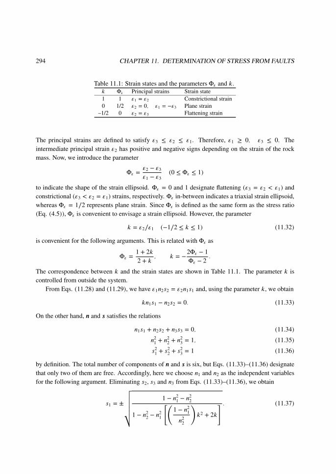
Table 11.1: Strain states and the parameters Φε and k.k Φε Principal strains Strain state1 1 ε1 = ε2 Constrictional strain0 1/2 ε2 = 0, ε1 = −ε3 Plane strain
–1/2 0 ε2 = ε3 Flattening strain
The principal strains are defined to satisfy ε3 ≤ ε2 ≤ ε1. Therefore, ε1 ≥ 0, ε3 ≤ 0. Theintermediate principal strain ε2 has positive and negative signs depending on the strain of the rockmass. Now, we introduce the parameter
Φε =ε2 − ε3
ε1 − ε3(0 ≤ Φε ≤ 1)
to indicate the shape of the strain ellipsoid. Φε = 0 and 1 designate flattening (ε3 = ε2 < ε1) andconstrictional (ε3 < ε2 = ε1) strains, respectively. Φε in-between indicates a triaxial strain ellipsoid,whereas Φε = 1/2 represents plane strain. Since Φε is defined as the same form as the stress ratio(Eq. (4.5)), Φε is convenient to envisage a strain ellipsoid. However, the parameter
k = ε2/ε1 (−1/2 ≤ k ≤ 1) (11.32)
is convenient for the following arguments. This is related with Φε as
Φε =1 + 2k2 + k
, k = −2Φε − 1Φε − 2
.
The correspondence between k and the strain states are shown in Table 11.1. The parameter k iscontrolled from outside the system.
From Eqs. (11.28) and (11.29), we have ε1n2s2 = ε2n1s1 and, using the parameter k, we obtain
kn1s1 − n2s2 = 0. (11.33)
On the other hand, n and s satisfies the relations
n1s1 + n2s2 + n3s3 = 0, (11.34)
n21 + n
22 + n
23 = 1, (11.35)
s21 + s
22 + s
23 = 1 (11.36)
by definition. The total number of components of n and s is six, but Eqs. (11.33)–(11.36) designatethat only two of them are free. Accordingly, here we choose n1 and n2 as the independent variablesfor the following argument. Eliminating s2, s3 and n3 from Eqs. (11.33)–(11.36), we obtain
s1 = ±
√√√√√√√1 − n2
1 − n22
1 − n22 − n2
1
[(1 − n2
1
n22
)k2 + 2k
] . (11.37)
11.8. RECHES’ MODEL 295
The eliminated values s2, s3 and n3 are calculated using the four equations, i.e., s is linked with n
through the orthorhombic symmetry. Once the two variables n1 and n2 are specified, the fault activityto accommodate the prescribed strain is constrained.
The next problem is how the variables n1 and n2 are chosen. To solve this problem, we assumethat the frictional resistance
τR = τ0 + (tanφ) σN (11.38)
works on a fault plane with the parameters τ0 and φ common to all faults. Namely, while a fault ismoving, the shear stress on the fault plane is equal to
σS = τR (11.39)
Note that the rock mass is assumed to be isotropic. Therefore, the principal axes of stress coincidewith the coordinate system, and the normal and shear stresses satisfy the following relationship withprincipal stresses:
σN = t(n) · n = σ1n21 + σ2n
22 + σ3n
23, (11.40)
σS = t(n) · s = σ1n1s1 + σ2n2s2 + σ3n3s3. (11.41)
Rearranging Eqs. (11.33)–(11.41), we obtain(σ1 − σ3
) (n1s1 − n2
1 tanφ)+(σ2 − σ3
) (kn1s1 − n2
2 tanφ)= τ0 + (tanφ)σ3. (11.42)
This relationship is satisfied when a fault is slipping.We have assumed a uniform spacing between faults. Consider a set to have n faults within a cube
that has a unit length of sides. If one of the faces of the cube is parallel to the faults, the spacingequals 1/n. Since the engineering shear strain of the cube is γ, the displacement of each fault is γ/n.The cube deforms in a similar way to a deck of cards. The n faults move by the distance γ/n againstthe resisting force τR × (unit area) = τR. Therefore, the energy dissipation by the n faults within theunit volume of the cube is
w = σSγ. (11.43)
Combining Eqs. (11.28), (11.33), (11.34), (11.41) and (11.43), we obtain the total dissipation dueto the four sets in a unit volume The four sets of faults dissipate in a unit volume of the rock mass
4w = 4σSγ = 4(σ1n1s1 + σ2n2s2 + σ3n3s3
) · ε1
4n1s1
=[σ1n1s1 + σ2n2s2 + σ3n3s3 − (σ3n1s1 + σ3n2s2 + σ3n3s3)
] ε1
n1s1
=[(σ1 − σ3
)n1s1 +
(σ2 − σ3
)n2s2
] ε1
n1s1
=[(σ1 − σ3) + (σ2 − σ3)k
]ε1.
296 CHAPTER 11. DETERMINATION OF STRESS FROM FAULTS
Accordingly, the total dissipation is proportional to the strain ε1. Let us define the symbol W todenote the constant of proportionality
W = (σ1 − σ3) + (σ2 − σ3)k. (11.44)
This is the dissipation for every incremental strain ∂(4w)/∂ε1 = W . Using Φ = (σ2 − σ3)/(σ1 − σ3)and Δσ = σ1 − σ3, Eq. (11.44) is rewritten as
W = (1 + Φk)Δσ (11.45)
and Eq. (11.42) is rewritten as[(1 + Φk) n1s1 −
(n2
1 + Φn22
)tanφ
]Δσ = τ0 + (tanφ)σ3. (11.46)
The friction is thought to be dependent on confining pressure (Eq. (11.38)), so we regard σ3 as avariable controlled from outside this system instead of the confining pressure.
Since there are pre-existing fractures with various orientations in the rock mass, some of whichare chosen as faults, then the faults that can be activated by the minimum differential stress may bechosen. The right-hand side of Eq. (11.46) and Δσ are, by definition, positive in sign. In addition,the right-hand side is given. Hence, the minimization of Δσ is achieved by determining the optimalcombination of n1, n2 and Φ that maximizes the content of the brackets in the left-hand side of Eq.(11.46). We have the analytical solutions for the cases k = −1/2, 0 and 1.
Constrictional strain is represented by k = 1. Then, the stress tensor and the fault sets areexpected to have axial symmetry. Therefore,
σ1 = σ2, n1 = n2. (11.47)
Substituting these into Eq. (11.37), we have
s1 =
√1 − 2n2
1
2. (11.48)
Substituting Eqs. (11.47) and (11.48) into Eqs. (11.45) and (11.46), we obtain
2Δσ = W, (11.49)
2Δσ
⎛⎝n1
√1 − 2n2
1
2− n2
1 tanφ
⎞⎠ = τ0 + (tanφ)σ3. (11.50)
Therefore, the dissipation W is minimized when Δσ is minimized (Eq. (11.49)). The optimal n1 isobtained by maximizing the content of the parentheses in the left-hand side of Eq. (11.50). Solvingthe equation
ddn
⎛⎝n1
√1 − 2n2
1
2− n2
1 tanφ
⎞⎠ =
√1 − 3n1
2(1 − 2n1)− 2n1 tanφ = 0,

11.8. RECHES’ MODEL 297
and using Eqs. (11.47) and (11.48), we obtain the fault orientation and slip direction of the case ofconstrictional strain:
n1 =12
√1 − sinφ, n2 = n1, s1
12
√1 + sinφ. (11.51)
Plane strain is indicated by k = 0 and ε2 = 0. Due to the symmetry,
n2 = 0. (11.52)
Combining Eqs. (11.37) and (11.52), we have
s1 =√
1 − n21 (11.53)
and combining Eqs. (11.45) and (11.46), we obtain
Δσ = W, (11.54)
Δσ
(n1
√1 − n2
1 − n21 tanφ
)= τ0 + (tanφ)σ3. (11.55)
Δσ fluctuates with W , again. Similar to the above discussion, it is found that the minimum Δσrequires
n1 =
√2
2
√1 − sinφ, n2 = 0, s1 =
√2
2
√1 − sinφ. (11.56)
Flattening is indicated by k = −1/2 and ε2 = ε3. Due to symmetry, we have
n2 = n3, σ2 = σ3. (11.57)
Combining Eqs. (11.35), (11.37) and (11.57),
n1 =√
1 − 2n22, s1 =
√3(1 − n2
1). (11.58)
In this case, we have
Δσ = W, (11.59)
Δσ
(n1
√1 − n2
1 − n21 tanφ
)= τ0 + (tanφ)σ3. (11.60)
Δσ is minimized when
n1 =
√2
2
√1 − sinφ, n2 =
12
√1 + sinφ, s1 =
√2
2
√1 + sinφ. (11.61)
Interestingly, the three cases have a common minimum differential stress, which is obtained fromEqs. (11.49)–(11.51), (11.54)–(11.56) and (11.59)–(11.61):
Δσmin =2 cosφ
1 − sinφ[τ0 + (tanφ)σ3] . (11.62)
298 CHAPTER 11. DETERMINATION OF STRESS FROM FAULTS
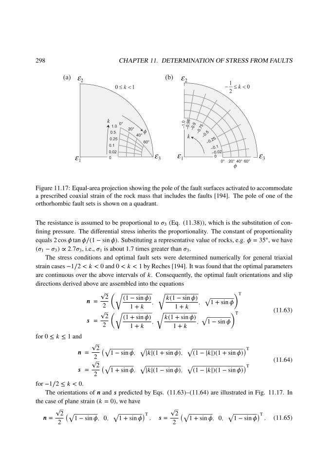
Figure 11.17: Equal-area projection showing the pole of the fault surfaces activated to accommodatea prescribed coaxial strain of the rock mass that includes the faults [194]. The pole of one of theorthorhombic fault sets is shown on a quadrant.
The resistance is assumed to be proportional to σ3 (Eq. (11.38)), which is the substitution of con-fining pressure. The differential stress inherits the proportionality. The constant of proportionalityequals 2 cosφ tanφ/(1 − sinφ). Substituting a representative value of rocks, e.g. φ = 35◦, we have(σ1 − σ3) ∝ 2.7σ3, i.e., σ1 is about 1.7 times greater than σ3.
The stress conditions and optimal fault sets were determined numerically for general triaxialstrain cases −1/2 < k < 0 and 0 < k < 1 by Reches [194]. It was found that the optimal parametersare continuous over the above intervals of k. Consequently, the optimal fault orientations and slipdirections derived above are assembled into the equations
n =
√2
2
(√(1 − sinφ)
1 + k,
√k(1 − sinφ)
1 + k,√
1 + sinφ
)T
s =
√2
2
(√(1 + sinφ)
1 + k,
√k(1 + sinφ)
1 + k,√
1 − sinφ
)T (11.63)
for 0 ≤ k ≤ 1 and
n =
√2
2
(√1 − sinφ,
√|k|(1 + sinφ),
√(1 − |k|)(1 + sinφ)
)T
s =
√2
2
(√1 + sinφ,
√|k|(1 − sinφ),
√(1 − |k|)(1 − sinφ)
)T(11.64)
for −1/2 ≤ k < 0.The orientations of n and s predicted by Eqs. (11.63)–(11.64) are illustrated in Fig. 11.17. In
the case of plane strain (k = 0), we have
n =
√2
2
(√1 − sinφ, 0,
√1 + sinφ
)T, s =
√2
2
(√1 + sinφ, 0,
√1 − sinφ
)T, (11.65)
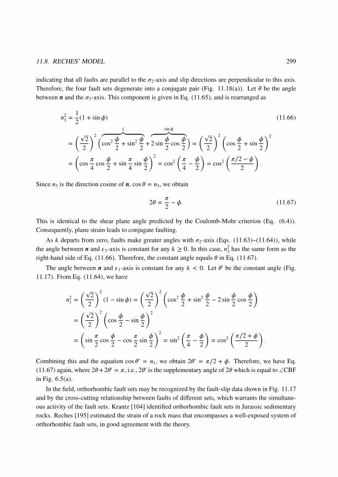
11.8. RECHES’ MODEL 299
indicating that all faults are parallel to the σ2-axis and slip directions are perpendicular to this axis.Therefore, the four fault sets degenerate into a conjugate pair (Fig. 11.18(a)). Let θ be the anglebetween n and the σ3-axis. This component is given in Eq. (11.65), and is rearranged as
n23 =
12
(1 + sinφ) (11.66)
=
(√2
2
)2 ( 1︷ ︸︸ ︷cos2 φ
2+ sin2 φ
2+
sinφ︷ ︸︸ ︷2 sin
φ
2cos
φ
2
)=
(√2
2
)2(cos
φ
2+ sin
φ
2
)2
=
(cos
π
4cos
φ
2+ sin
π
4sin
φ
2
)2
= cos2(π
4− φ
2
)= cos2
(π/2 − φ
2
).
Since n3 is the direction cosine of n, cos θ = n3, we obtain
2θ =π
2− φ. (11.67)
This is identical to the shear plane angle predicted by the Coulomb-Mohr criterion (Eq. (6.4)).Consequently, plane strain leads to conjugate faulting.
As k departs from zero, faults make greater angles with σ2-axis (Eqs. (11.63)–(11.64)), whilethe angle between n and ε3-axis is constant for any k ≥ 0. In this case, n2
3 has the same form as theright-hand side of Eq. (11.66). Therefore, the constant angle equals θ in Eq. (11.67).
The angle between n and ε1-axis is constant for any k < 0. Let θ′ be the constant angle (Fig.11.17). From Eq. (11.64), we have
n21 =
(√2
2
)2
(1 − sinφ) =(√
22
)2(cos2 φ
2+ sin2 φ
2− 2 sin
φ
2cos
φ
2
)=
(√2
2
)2(cos
φ
2− sin
φ
2
)2
=
(sin
π
2cos
φ
2− cos
π
2sin
φ
2
)2
= sin2(π
4− φ
2
)= cos2
(π/2 + φ
2
).
Combining this and the equation cos θ′ = n1, we obtain 2θ′ = π/2 + φ. Therefore, we have Eq.(11.67) again, where 2θ+2θ′ = π, i.e., 2θ′ is the supplementary angle of 2θ which is equal to ∠CBFin Fig. 6.5(a).
In the field, orthorhombic fault sets may be recognized by the fault-slip data shown in Fig. 11.17and by the cross-cutting relationship between faults of different sets, which warrants the simultane-ous activity of the fault sets. Krantz [104] identified orthorhombic fault sets in Jurassic sedimentaryrocks. Reches [195] estimated the strain of a rock mass that encompasses a well-exposed system oforthorhombic fault sets, in good agreement with the theory.
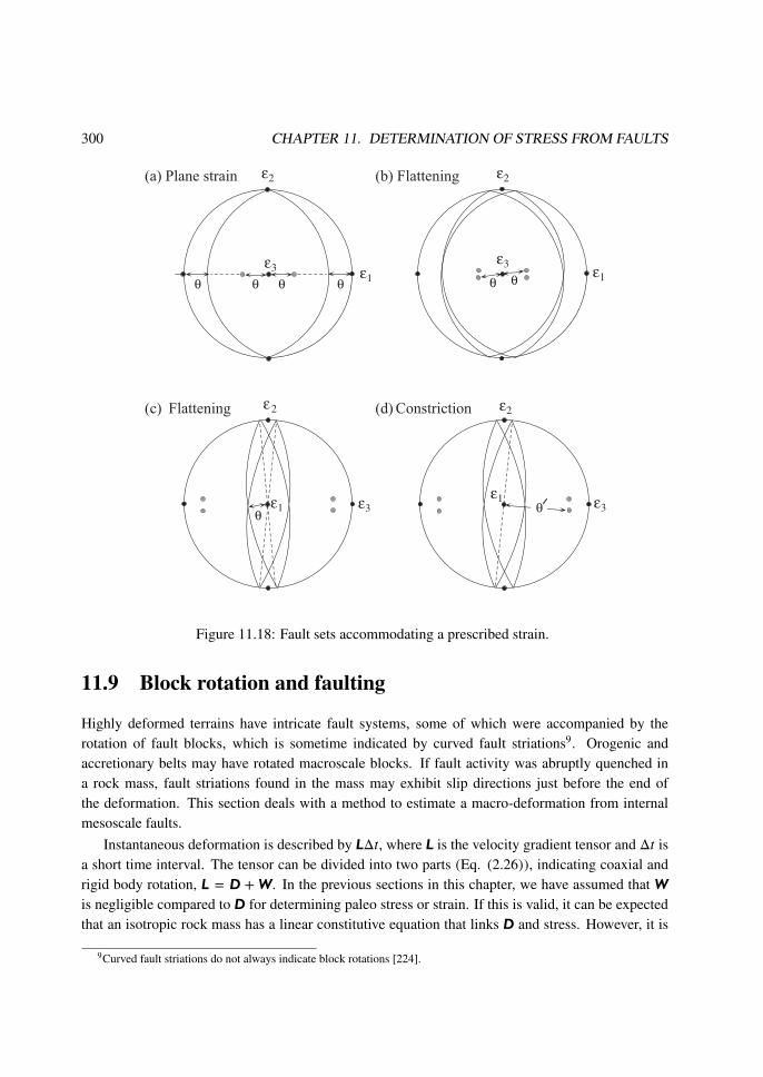
300 CHAPTER 11. DETERMINATION OF STRESS FROM FAULTS
Figure 11.18: Fault sets accommodating a prescribed strain.
11.9 Block rotation and faulting
Highly deformed terrains have intricate fault systems, some of which were accompanied by therotation of fault blocks, which is sometime indicated by curved fault striations9. Orogenic andaccretionary belts may have rotated macroscale blocks. If fault activity was abruptly quenched ina rock mass, fault striations found in the mass may exhibit slip directions just before the end ofthe deformation. This section deals with a method to estimate a macro-deformation from internalmesoscale faults.
Instantaneous deformation is described by LΔt, where L is the velocity gradient tensor and Δt isa short time interval. The tensor can be divided into two parts (Eq. (2.26)), indicating coaxial andrigid body rotation, L = D + W. In the previous sections in this chapter, we have assumed that Wis negligible compared to D for determining paleo stress or strain. If this is valid, it can be expectedthat an isotropic rock mass has a linear constitutive equation that links D and stress. However, it is
9Curved fault striations do not always indicate block rotations [224].
11.9. BLOCK ROTATION AND FAULTING 301
the present problem to incorporate the rotation in the fault striation analysis.To this end, the Twiss-Protzman-Hurst model utilizes the mechanics of micropolar continua
[249]. Micropolar continua are physically idealized macroscopic continua that have microscopicrigid particles and can model such substances as liquid crystals, rigid suspensions, concrete withsand, and muddy fluids. Within the present context, the rigid particles simulate fault blocks that canrotate. The mechanics of micropolar continua is beyond the scope of this book. Interested readerscan consult textbooks [58, 128]. Here, the results of the Twiss-Protzman-Hurst model is brieflyintroduced [249].
Micropolar continua is a limited version of micromorphic continua that has deformable mi-crostructures. The mechanics of micromorphic continua has macro and micro fields of kinematicvariables including position, velocity, and rotation. The macro velocity gradient tensor is written asusual: L = D + W. The micro velocity gradient tensor is also defined as L = D + W, i.e., we distin-guish macro and micro quantities by overlines. Fault blocks are assumed to be rigid so that we usethe mechanics of micropolar continua. Then we have D = O, and the micro velocity gradient tensorequals the micro spin tensor (L = W). Here, the principal values of D are numbered in descendingorder, D1 ≥ D2 ≥ D3. Obviously,
12ΔD ≡ 1
2
(D1 −D3
)is the maximum shearing rate, just like the maximum shear stress equals half the differential stress.The dimensionless quantity
ΦD ≡ D2 −D3
D1 −D3
(0 ≤ ΦD ≤ 1)
designates the shape of the instantaneous strain ellipsoid. Here, elongation is positive so that ΦD = 0and 1 indicate constriction and flattening, respectively. ΦD = 1/2 corresponds to plane strain.
Taking the principal axes of D to define the rectangular Cartesian coordinates O-123, the max-imum shear rate is on the O-13 plane. The non-diagonal components of a spin tensor make up avorticity vector (Eq. (2.43)), and the vorticity is related to an angular velocity (Eq. (2.44)). Themacro and micro angular velocities within the O-13 plane are equal to W 13 and W13, respectively.
The quantity(W 13 −W13
)indicates the difference in the velocities. Accordingly, we define the
dimensionless number
Ω ≡ W 13 −W13
ΔD/2to indicate the difference.
Let N be the outward unit normal to a small part on the surface of a fault block. The surface isrubbed by the relative velocity of the surface of the neighboring block. Twiss et al. [249] derivedthe direction of the resultant striae, being parallel to the vector
v =
⎛⎝ 1 −N21 − ΦDN
22
ΦD −N21 − ΦDN
22
−N21 − ΦDN
22
⎞⎠T⎛⎝N1
N2
N3
⎞⎠ +Ω2
⎛⎝ N3
0−N1
⎞⎠ . (11.68)

302 CHAPTER 11. DETERMINATION OF STRESS FROM FAULTS
Figure 11.19: Tangent-lineation diagrams showing fault-slip data predicted by the Twiss-Protzman-Hurst model with different Ω and the same ΦD = 0.5 and the same principal axes of D [249]. TheD-axis indicates the orientation of the maximum instantaneous elongation.
Given the dimensionless numbers ΦD and Ω, the striating direction is calculated with this equationfor any surface with N . If the micro rotation is quenched by the cessation of macro deformation, thestriation on the surface of fault blocks may give constraints to the kinematic parameters ΦD and Ωand the principal orientations of D.
The fault-slip data predicted by this model is shown in Fig. 11.19. The tangent-lineation dia-grams in Fig. 11.5 show the fault-slip data specifically for the case of Ω = 0. When |Ω| is small, thegross pattern in the tangent-lineation diagram is similar to that of the case of Ω = 0. However, it nolonger has the orthorhombic symmetry but makes up a triclinic system. For a large Ω, arrows in thetangent-lineation diagram show a rotational pattern about D2-axis.
Exercises
11.1 Suppose a rock mass that is cut by a great number of conjugate sets of small-scale faults.Show that the strain of the mass caused by the internal fault activities is a plain strain. Assume thatthe orientation of stress axes does not change in the body, and that faulting are generated followingthe Coulomb-Navier criterion.
11.2 Show that the point S in Fig. 11.3 moves from S0 to S1 with an increase of ΦB from 0 to1, where the points S0 and S1 represent the orientation of the σ1 and σ3 axes, respectively, on thestereonet.
11.3 Verify that the σ1-axis with a specific stress ratio Φ is constrained by a fault-slip datum to bein the region to the left of the dotted line in the stereonet in Fig. 11.7.