DETERMINATION OF STATIC STIFFNESS OF MECHANICAL...

DETERMINATION OF STATIC STIFFNESSOF MECHANICAL STRUCTURESFROM OPERATIONAL MODAL ANALYSIS

A. Melnikov 1, K. Soal 2, J. Bienert 3

1 Mr, Technische Hochschule Ingolstadt, Germany, [email protected] Mr, Stellenbosch University, South Africa, [email protected] Prof, Technische Hochschule Ingolstadt, Germany, [email protected]

ABSTRACTThe experimental determination of static stiffness is an important task in structural design. The twocurrent methods include clamping the structure, applying pre-defined loads, and measuring the displace-ments, or performing EMA and interpolating the frequency response function to 0 Hz. Both methodsrequire high experimental effort in laboratory setup. This paper presents a new idea, whereby the struc-ture is measured during normal operating conditions, and OMA is used to reconstruct the stiffness matrix.The challenge of unscaled eigenvectors in operational modal analysis is overcome using mass modifica-tion scaling, whereby the structure is measured at a baseline and mass modified condition.Three different models were investigated: a basic discrete model, a laboratory ladder frame and a carbody. Investigations were conducted into the effects of the position and magnitude of the mass mod-ification, the number of assigned degrees of freedom of the system, the mode shape error effect andthe effect of modal truncation. Key findings include significantly reduced reconstruction errors whenthe mass modification is a scalar multiple of the mass matrix. It was also found that the accuracy ofthe reconstructed stiffness matrix is strongly dependent on the uncertainty in the eigenvectors, as wellas how the model is truncated. A finite element model of the ladder frame was used to test differentmodification strategies and to compare to results from operational modal analysis. A key finding whichwas not revealed by the discrete model was the importance of including the RBM in the stiffness matrixreconstruction. Finally experimental modal analysis and operational modal analysis were conducted onan Audi TT. The reconstructed stiffness matrices, bending and torsion static stiffness are then comparedand discussed.

Keywords: operational modal analysis, oma, measurement, static stiffness, car, body in white, biw, audi

1. INTRODUCTION

The dynamic behavior of most mechanical structures is fundamentally linked to their performance. Thecreation of mathematical models which can explain these physical responses is therefore key in the designand optimization process. The automotive industry provides such an example, where the vehicle chassisplays an integral role in the vehicle dynamics - handling, steering and road holding ability and in NoiseVibration Harshness (NVH) improvement. The chassis is also responsible for housing and linking themain elements - engine, wheels and drive train, and is a crucial safety barrier for the vehicle occupants.Two important metrics are the chassis bending and torsional stiffness, which can be calculated eitheranalytically or experimentally. Analytical methods are limited by complex geometries, materials andjoints, often requiring thorough experimental validation and updating. The two current experimentaltechniques include clamping the structure, applying pre-defined loads, and measuring the displacements,or performing experimental modal analysis and interpolating the frequency response function to 0 Hz.Both methods require high experimental effort in laboratory setup.

This paper presents a new idea, whereby the structure is measured during normal operating conditions,and Operational Modal Analysis (OMA) is used to reconstruct the stiffness matrix. The challenge ofunscaled eigenvectors in OMA is overcome using mass modification scaling, whereby the structure ismeasured at a baseline and mass modified condition. The mathematics of the reconstruction techniqueare presented first, followed by a discrete model simulation investigating the error effects of various massmodification configurations. The technique is then applied to a laboratory ladder frame structure. A finiteelement model of the ladder frame was also created and is compared to the experimental results. Finallythe technique is applied to a vehicle chassis Body in White (BIW).

2. FUNDAMENTAL IDEA

2.1. Basic equations

As a starting point the discrete Multiple Degree of Freedom (MDOF) ordinary differential equation inthe notation

Mx + Bx + Kx = f(t) (1)

is used, whereby M represents the mass matrix, B the damping matrix and K the stiffness matrix. Inmost engineering applications, for example in large steel structures, the damping part can be suppressedand the system of equations becomes much easier leading to the eigenvalue problem

KΦ = MΦΛ. (2)

The matrix Λ is a diagonal matrix and contains the eigenvalues corresponding with the position of theeigenvectors in the matrix Φ. Alternatively the state space notation can be used to include general viscousdamping into the equation by including of the momentum balance. This leads to the following eigenvalueproblem with twice the number of Degrees of Freedom (DOFs)

A0Φ = A1ΦΛ (3)

which can be solved like the undamped case in Equation 2. For reasons of simplicity the notation ofundamped systems will be used in the following discussion, which can be expanded to damped systemsbased on the state space formulation.

The mass normalization of the eigenvectors is an important procedure to access the complete set ofproperties of the modal matrix. The calculation step can be done in the following way

Φ = Ψ[ΨTMΨ]−1/2. (4)

In this case Φ represents for the modal matrix of mass-normalized eigenvectors and Ψ the matrix ofarbitrarily scaled eigenvectors.

Based on Equation 2 and including the mass normalization of the eigenvectors from Equation 4 the massand stiffness matrices can be reconstructed from the formulation

ΦTMΦ = I

ΦTKΦ = Λ(5)

by inverting the modal matrix Φ and multiplying it from right and left, it leads directly to the mass andstiffness matrices

M = (ΦT )−1IΦ−1

K = (ΦT )−1ΛΦ−1.(6)

The inversion of the modal matrix becomes more complicated when the number of DOFs and the numberof modes are different. In this case the use of the pseudo inverse is necessary. The general formulationuses the Singular Value Decomposition (SVD) to obtain the pseudo inverse in the following form

Φ = USV H

Φ+ = V S+UH .(7)

2.2. Mode shape rescaling and matrix reconstruction

There is no direct method to obtain the normalized shape vectors from OMA, however there are a fewapproaches of how to approximate it. These methods are mostly based on the sensitivity of eigenfrequen-cies and mode shapes described by DRESIG in [1] with the following conditions: eigenvector remainswithin modification

∆xi ≈ 0 (8)

and small mass change

‖∆M‖ �‖M‖ . (9)

A Sensitivity-based method to estimate the scaling factors was presented by PARLOO in [2] and wasvalidated on a full scale bridge in subsequent years [3]. The frequency shifts between the original andmass-modified system were used for re-scaling (mass-normalizing) of the mode shapes. Later the for-mulation of PARLOO was established as [4]

α =

√2∆ω

ωxT∆Mx(10)

and the formulation of BRINCKER, with only small differences was establishes as

α =

√ω21 − ω2

2

ω22x

T∆Mx. (11)

For easier use the BRINCKER formulation can be used in matrix form as

A = [(Λ−Λm)(diag{ΨT∆MΨ}Λm)−1]12 (12)

with the diagonal matrix A containing the scaling factors α. The rescaling can be done by multiplyingthe factors by the eigenvectors to obtain an approximation of the modal matrix

Φ ≈ Φ = ΨA (13)

where it must be remembered that the quality depends on the fulfillment of Equations 8 and 9. Thesystem matrices can then be reconstructed by

Mr = (ΦT )+IΦ+

Kr = (ΦT )+ΛΦ+(14)

using two OMA data sets - an original or baseline and a mass modified system.

3. DISCRETE MODEL

For testing purposes a simple discrete model with 5 DOFs was created as shown in Figure 1.

mk k k km m m m

Figure 1: Simple undamped 5 degrees of freedom system with one Rigid Body Mode/s (RBM)

The model consists of 5 equal masses connected by 4 springs with equal stiffness and can move only inone direction. Analyzing the model leads to one RBM, which was chosen to show the functionality ofthe method independent of RBM. The complete set of mode shapes is shown in Figure 2.

54321

Mode shape 3 by 5.91655 Hz

5

1 2 3 4 5

4321


5432


1

Mode shape 1 by 0 Hz

54321


Figure 2: Complete set of mode shapes for basic discrete model.

3.1. Results for different system setups

There are a number of ways to setup the system, which have an effect on the quality of the results. Theerrors obtained by applying a single 1% mass modification at one degree of freedom and varying itsposition are shown in the Figure 3. The highest error is present when the mass modification is located at

rela

tive e

rror

mass modification position

0.7

0.6

0.5

0.4

0.3

0.2

0.1

05432

mass error

stiffness error

1

Relative error estimation

Figure 3: Global relative error for mass and stiffness.

the center node. This becomes obvious when considering Figure 2 since the center node is located at avibration nodal point for modes 2 and 4, and therefore the mass modification does not contribute to thefrequency shift of these modes.

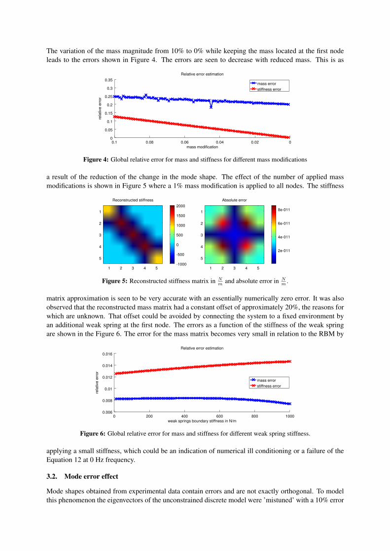
The variation of the mass magnitude from 10% to 0% while keeping the mass located at the first nodeleads to the errors shown in Figure 4. The errors are seen to decrease with reduced mass. This is as


rela

tive e

rror

mass modification

0.35

0.3

0.25

0.2

0.15

0.1

0.05

0

0.1 0.08 0.06 0.04 0.02

mass error

stiffness error

0

Figure 4: Global relative error for mass and stiffness for different mass modifications

a result of the reduction of the change in the mode shape. The effect of the number of applied massmodifications is shown in Figure 5 where a 1% mass modification is applied to all nodes. The stiffness

Absolute errorReconstructed stiffness

1 2 3 4 5

1

2

3

4

5

-1000

-500

0

1000

1500

2000

1 2 3 4 5

1

2

3

4

5

2e-011

4e-011

6e-011

8e-011

500

Figure 5: Reconstructed stiffness matrix in Nm and absolute error in N

m .

matrix approximation is seen to be very accurate with an essentially numerically zero error. It was alsoobserved that the reconstructed mass matrix had a constant offset of approximately 20%, the reasons forwhich are unknown. That offset could be avoided by connecting the system to a fixed environment byan additional weak spring at the first node. The errors as a function of the stiffness of the weak springare shown in the Figure 6. The error for the mass matrix becomes very small in relation to the RBM by


rela

tive e

rror

weak springs boundary stiffness in N/m

0.016

0.014

0.012

0.01

0.008

0.0061000800600400200

mass error

stiffness error

0

Figure 6: Global relative error for mass and stiffness for different weak spring stiffness.

applying a small stiffness, which could be an indication of numerical ill conditioning or a failure of theEquation 12 at 0 Hz frequency.

3.2. Mode error effect

Mode shapes obtained from experimental data contain errors and are not exactly orthogonal. To modelthis phenomenon the eigenvectors of the unconstrained discrete model were ’mistuned’ with a 10% error

of random sign for every entry. Using these eigenvectors for the reconstruction led to the stiffness matrixshown in the Figure 7. The structure of the original stiffness matrix is still recognizable, but there are


1 2 3 4 5

1

2

3

4

5 -1000

0

1000

2000

1 2 3 4 5

1

2

3

4

5 100

200

300

400

500

600

Figure 7: Reconstructed stiffness matrix in Nm and absolute error in N

m .

locally high errors for some entries. The reconstruction procedure is therefore sensitive to the modeshape errors.

3.3. Modal truncation

To investigate the influence of modal truncation one of the five modes were rejected from the reconstruc-tion. The stiffness matrices with the errors are shown in the following Figures 8 and 9. The truncation of


1 2 3 4 5

1

2

3

4

5

-1000

-500

0

1000

1500

2000

1 2 3 4 5

1

2

3

4

5

5

10

15

20

500

Figure 8: Truncation of the mode 1: reconstructed stiffness matrix in Nm and absolute error in N

m .


1 2 3 4 5

1

2

3

4

5

-500

0

500

1000

1 2 3 4 5

1

2

3

4

5200

400

600

800

1000

1200

1400

Figure 9: Truncation of the mode 5: reconstructed stiffness matrix in Nm and absolute error in N

m .

mode 1, which is the RBM had no effect on the reconstructed matrix, leading to the conclusion that thismode is superfluous in this basic model. The truncation of mode 5, which is the highest mode completelydestroys the result. The errors between mode 1 and mode 5 truncation lie between these extremes, alsodescribed in [5]. The higher modes are therefore of greater importance for the quality of the reconstructedstiffness matrix.

4. LABORATORY LADDER FRAME

Investigations of a ladder frame shown in the Figure 10, were conducted as a first laboratory testing step.The frame was attached by weak springs to a fixed environment and the measurements were conductedusing accelerometers at 6 locations. The geometry and measurement point positions are described in [5].

Figure 10: Ladder frame experimental set-up.

4.1. Finite Element Method (FEM) evaluation

The ladder frame was modeled with FEM and 20 modes were identified with the natural frequenciespresented in the Table 1. The stiffness matrix shown in the Figure 11 was extracted from the FEM

Table 1: FEM calculated frequencies.

Mode Frequenzy (Hz) Mode Frequency (Hz)

1 0.46330 · 10−1 11 518.142 0.50765 · 10−1 12 588.053 0.64566 · 10−1 13 611.434 43.049 14 727.705 244.46 15 802.406 254.54 16 841.367 274.41 17 845.578 310.14 18 863.109 383.85 19 900.0210 416.29 20 1000.5

model, and was used as the reference stiffness matrix. Four different mass modification strategies were

FEM stiffness matrix

1 2 3 4 5 6

1

2

3

4

5

6 -200

0

200

400

Figure 11: Extracted stiffness matrix from the FEM in Nmm .

analyzed using the FEM model. Modification with 156g at the Degree of Freedom (DOF) 1, symmetricalmodification at DOF 1 and 4 with 2 × 156g and 2 × 40g and a modification with 156g at all six pointswere applied. The results are presented in Table 2, were it can be seen that cases 2 and 3 are not in

the appropriate range. The reasons are in the validation of the requirements set by the Equations 8 and9. The results of case 5 show the smallest error, since the mass modification matrix is close to a scalarmultiple of the original mass matrix.

∆M = a ·M , a ∈ <, a > 0 (15)

4.2. OMA with single mass modification

OMA was conducted for the single mass modification with 156g at the DOF 1 and the reconstructedstiffness matrix is shown in Figure 12. The structure of the two 3× 3 diagonal blocks shows correlationwith the FEM calculated reference, however the off-diagonal blocks are different and the values arehigher than expected. A reason for the differences between the measurements and the FEM model isexpected to be as a result of the single point mass modification of large mass magnitude together withthe weakness of the OMA and FEM analysis. The corner joints in the FEM were modeled as mass pointswithout stiffness and damping properties and are therefore also expected to introduce errors. The resultsof the OMA reconstruction are presented and compared to the FEM reconstructions in Table 2.

absolute error to FEMOMA stiffness matrix

1 2 3 4 5 6

1

2

3

4

5

6-500

0

500

1000

1 2 3 4 5 6

1

2

3

4

5

6 200

300

400

500

600

700

Figure 12: Reconstructed OMA stiffness matrix Kr in Nmm and absolute error in N

mm (FEM reference).

Table 2: Ladder frame static stiffnesses gained by different mass modification approaches and technology.

Case Bend. Nmm B. error % Tors. N ·m

rad T. error %

1 FEM reference 906.79 - 695.19 -2 FEM 1× 156g 686.56 24.286 816.03 17.3833 FEM 2× 156g 554.93 38.803 374.83 46.0834 FEM 2× 40g 964.60 6.3746 712.01 2.41995 FEM 6× 156g 962.73 6.1685 698.17 0.42926 OMA 1× 156g 1026.7 13.225 1201.6 72.856

5. ADVANCED MODEL - VEHICLE BODY

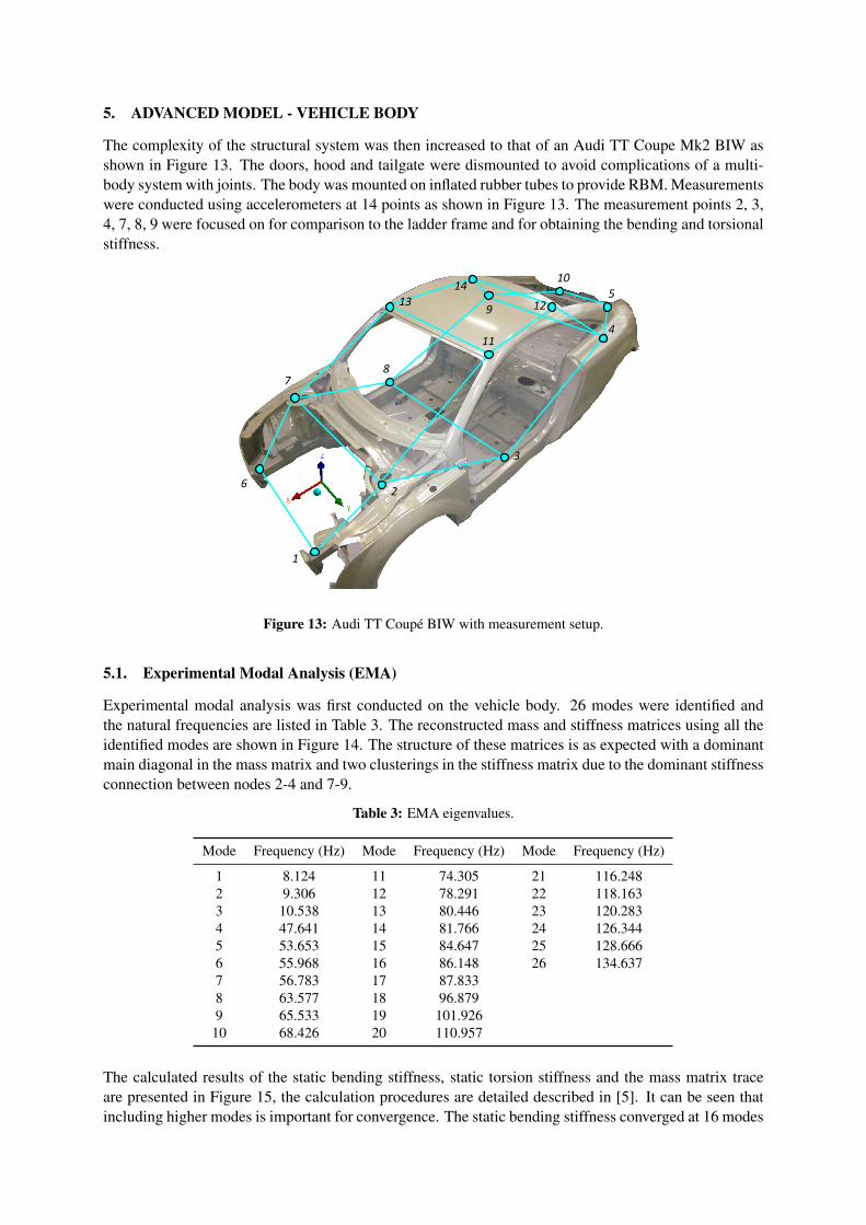
The complexity of the structural system was then increased to that of an Audi TT Coupe Mk2 BIW asshown in Figure 13. The doors, hood and tailgate were dismounted to avoid complications of a multi-body system with joints. The body was mounted on inflated rubber tubes to provide RBM. Measurementswere conducted using accelerometers at 14 points as shown in Figure 13. The measurement points 2, 3,4, 7, 8, 9 were focused on for comparison to the ladder frame and for obtaining the bending and torsionalstiffness.

1

2

3

4

5

6

7 8

9

10

11

12 13

14

Figure 13: Audi TT Coupé BIW with measurement setup.

5.1. Experimental Modal Analysis (EMA)

Experimental modal analysis was first conducted on the vehicle body. 26 modes were identified andthe natural frequencies are listed in Table 3. The reconstructed mass and stiffness matrices using all theidentified modes are shown in Figure 14. The structure of these matrices is as expected with a dominantmain diagonal in the mass matrix and two clusterings in the stiffness matrix due to the dominant stiffnessconnection between nodes 2-4 and 7-9.

Table 3: EMA eigenvalues.

Mode Frequency (Hz) Mode Frequency (Hz) Mode Frequency (Hz)

1 8.124 11 74.305 21 116.2482 9.306 12 78.291 22 118.1633 10.538 13 80.446 23 120.2834 47.641 14 81.766 24 126.3445 53.653 15 84.647 25 128.6666 55.968 16 86.148 26 134.6377 56.783 17 87.8338 63.577 18 96.8799 65.533 19 101.92610 68.426 20 110.957

The calculated results of the static bending stiffness, static torsion stiffness and the mass matrix traceare presented in Figure 15, the calculation procedures are detailed described in [5]. It can be seen thatincluding higher modes is important for convergence. The static bending stiffness converged at 16 modes

Mass matrixStiffness matrix

1 2 3 4 5 6

1

2

3

4

5

6-5e+006

0

5e+006

1e+007

1 2 3 4 5 6

1

2

3

4

5

6

0

20

40

60

Figure 14: Reconstructed EMA stiffness matrix Kr in Nm and mass matrix Mr in kg with full modal result set.

to approximately 20 kNmm . This is within the expected range from literature [6–8]. The static torsion

stiffness did not show clear convergence increasing to a final value of 144.94 kNdeg . This far exceeds the

value published by Audi of 28.5 kNdeg by 408%. The trace of the mass matrix converges at 13 modes to

296kg which is in the expected range.

5 10 15 20 25 3020406080

100120140160

Modes included

Stiffness in k

N/d

eg

Static torsion stiffness

5 10 15 20 25 300

1000

2000

3000

4000

5000

Modes included

Mass in k

g

Mass matrix trace

Static bending stiffness

Stiffness in

kN

/mm

Modes included

70

60

50

40

30

20

1030252015105

Figure 15: Static bending, static torsion stiffness and mass matrix trace as a function of the number of includedmodes.

5.2. OMA with Mass Modification

Operational modal analysis was then performed with random (in space and time) multi-point (2 person)tapping excitation. Mass modifications of ∼ 2.5 − 4.1kg =⇒ 0.8% − 1.4% of the total mass weremade at 6 DOFs (2 3 4 7 8 9), 2 DOFs (2 7) and 1 DOF (2) during consecutive tests in order to scalethe eigenvectors. It was found that due to the complexity (not in phase but in identifiable shape orsymmetry) of the resulting mode shapes, that it was very difficult to track and link the modal shift aftermass modification. Especially since the modes were closely spaced and did not all move by the sameamounts i.e. the order of the modes was changed. For this reason a reduced mode set of six identifiablemodes was used. The resulting reconstructed mass and stiffness matrices after modal scaling are shownin Figure 16

The mass matrix has a less dominant main diagonal, while the stiffness matrix retains most of the ex-pected matrix structure. The static stiffness results from both EMA and OMA are presented in Table 4.OMA with 6-mass scaling provided more accurate results than 2-mass and 1-mass scaling as expected

Mass matrixStiffness matrix

1 2 3 4 5 6

1

2

3

4

5

6-1e+007

0

1e+007

2e+007

1 2 3 4 5 6

1

2

3

4

5

6 -50

0

50

100

150

Figure 16: Reconstructed OMA stiffness matrix Kr in Nm and mass matrix Mr in kg with full modal result set.

from the discrete model. If it is however not possible to place masses at each measurement location forpractical reasons, certain points may provide better results, as shown by the 1-mass vs. 2-mass compar-ison. The large error in the torsion stiffness for EMA with full resolution is unclear. It was howeverseen that including higher modes was important to achieve convergence. The importance of includingthe RBM in the reconstruction can be seen in the poor results of case 3.

Table 4: Static stiffness results from EMA and OMA.

Case Bend. kNmm Tors. kNm

mm T. error %

1 EMA full res. 20.35 144.94 408.562 EMA 6-modes 167.71 26.15 8.263 EMA full no RBM 64.65 314.93 1005.04 OMA 6-masses 47.95 25.92 9.055 OMA 2-masses 3.55 13.64 52.136 OMA 1-mass 31.74 20.06 29.63

6. CONCLUSION

The determination of static stiffness from OMA reconstruction was tested and benchmarked. A basicdiscrete model was used to prove the concept and investigate the effects of the mass modification position,number of applied mass modifications and the size of the masses. It was found that reconstruction errorswere smallest when the mass modification is a scalar multiple of the mass matrix and the masses aremade as small as possible but as large as necessary to exceed measurement error. The reconstructionerrors were found to be strongly dependant on the uncertainty in the eigenvectors, as well as by how themodel was truncated - with the inclusion of higher modes significantly reducing the error.

A ladder frame structure was used to test the idea in the laboratory and a FE model was built to in-vestigate different modification strategies and to compare to results from OMA. Large errors resultedfrom the OMA reconstruction mainly due to the single mass modification and subsequently poor modeshape scaling. The revelation of the matrix structure could however still be an important factor for under-standing and investigating natural phenomena. Finally EMA and OMA were conducted on an Audi TTBIW, and the reconstructed stiffness matrices were used to calculate the bending and torsion static stiff-ness. Results showed convergence when increasing the number of modes included in the reconstruction.Accurate bending stiffness values were calculated from OMA reconstruction with 6-mass modification.The most accurate torsional stiffness values were calculated from EMA with a truncated 6 mode set.Importantly it was also found that the RBM played an insignificant role in the ladder frame stiffnessreconstruction but a significant role in the vehicle body reconstruction. The technique has shown muchpotential, but requires further research to quantify and improve the reconstruction error effects.

This method has been registered as patent DE 10 2015 208 613 A1 2016.11.10 [9].

REFERENCES

[1] Dresig, H. and F. Holzweißig (2012): Maschinendynamik. 11th ed. Springer Vieweg.[2] Parloo, E. et al. (2002): “Sensitivity-Based Operational Mode Shape Normalization”. In: Mechani-

cal Systems and Signal Processing:757–767.[3] Parloo, E. et al. (2005): “Sensitivity-Based Operational Mode Shape Normalization: Application to

a Bridge”. In: Mechanical Systems and Signal Processing:43–55.[4] Brincker, R. and P. Andersen (2003): “A Way of Getting Scaled Mode Shapes in Output Only

Modal Testing”. In: Processing of the 21st International Modal Analysis Conference (IMAC).[5] Melnikov, A. (2016): Determination of static stiffness from operational modal analysis, Masterthe-

sis. Technische Hochschule Ingolstadt.[6] Helsen, J. et al. (2010): “Global static and dynamic car body stiffness based on a single experimental

modal analysis test”. In: Proceedings of ISMA2010 including USD2010:2505–2522.[7] Sharanbasappa, E. S. Prasd, and P. Math (2016): “Global Stiffness Analysis of BIW Structure”. In:

International Journal of Research in Engineering and Technology 5:182–187.[8] Reichelt, M. (2003): Identifikation schwach gedämpfter Systeme am Beispiel von Pkw-Karosserien.

Fortschritt-Berichte VDI: Reihe 11, Schwingungstechnik, Lärmbekämpfung. VDI-Verlag.[9] Bienert, J. (2016): Verfahren zur experimentellen Bestimmung einer Steifigkeitsmatrix, einer Massen-

matrix und/oder einer Dämpfungsmatrix eines mechanischen Objekts. Pat. DE102015208613 A1.

DETERMINATION OF STATIC STIFFNESS OF MECHANICAL...

Documents

Transcript of DETERMINATION OF STATIC STIFFNESS OF MECHANICAL...