Determinants of interregional mobility in Russia:

evidence from panel data∇

Yuri Andrienko* and Sergei Guriev**

February 2003

Abstract The paper studies determinants of internal migration in Russia. Using panel data on gross

region-to-region migration flows in 1992-99, we estimate the effect of economic, political

and social factors. Although overall migration is rather low, it turns out that its intensity does

depend on economic factors even controlling for fixed effects for each origin-destination pair.

People move from poorer and job scarce regions with worse public good provision to ones

that are richer and more prospering both in terms of employment prospects and public goods.

Migration is however constrained by the lack of liquidity; for the poorest regions, an increase

in income raises rather than decreases outmigration. Our estimates imply that up to a third of

Russian regions are locked in poverty traps.

JEL Codes: P23, J61, P36, R23

Keywords: internal migration, liquidity constraints, gravity model, Russia's transition

∇ The authors thank John Earle, Guido Friebel, Stas Kolenikov, Vladimir Popov, Ekaterina Zhuravskaya, and participants of the CEFIR seminar and Russia2015 conference for discussion and helpful comments. We would also like to thank the organizers of the Russian Longitudinal Monitoring Survey (RLMS). * Centre for Economic and Financial Research (CEFIR), Moscow. E-mail: yandrienko@cefir.ru ** New Economic School and CEFIR. E-mail: sguriev@nes.ru

2

Non-technical summary Interregional labor mobility is one of the key issues in Russia’s transition to market economy.

To transform its economy, Russia has to reallocate resources from inefficient enterprises

established under the Soviet system to new sectors. This problem has an important regional

dimension: Russia has inherited a geographically concentrated industrial structure. Many

towns and even regions rely upon a single industry or, in some cases, a single enterprise.

Intersectoral reallocation of resources therefore requires interregional mobility of factors.

Since Russia still lacks mature capital market institutions, capital mobility is very low; capital

does not reallocate to regions with cheap and qualified labor. This is why geographical labor

mobility is vital to successful transition.

In this paper, we use panel data on region-to-region gross migration flows for 1992-99 to

estimate what determines interregional migration in modern Russia. We study the

characteristics of the source region that induce people to leave and the factors that attract

people in the destination areas. We test whether migration is explained by differentials in

income, unemployment, poverty, education, life expectancy, conflict, public good provision,

or inertia and legacies inherited from the Soviet time. In other words, we estimate whether

people ‘vote with their feet.’

We find that although the inertia and legacies do account for a substantial share of migration,

current economic performance and public goods provision also matter a great deal. Internal

migration depends upon income per capita, unemployment rate, poverty and public goods

provision in the intuitive way, even controlling for legacies, inertia, and macroeconomic

shocks. Our analysis implies that there is a Tiebout-type competition between Russian

regions. Regional policies that improve living standards, create jobs and improve public

goods provision, attract migrants. These effects are not large but substantial relative to

average migration rate. However, the overall migration rates are low both compared to other

countries and to the Soviet time. We show that liquidity constraints are an important barrier

to mobility. While the effect of income on outgoing migration is negative on average, it is

positive for poor regions. Although lower income makes people more willing to leave, it also

makes them less able to overcome the liquidity constraints and go. About a third of Russian

regions are locked in poverty traps which explains lack of convergence between rich and poor

regions. Hence, development of financial markets is crucial for strengthening the Tiebout

competition between Russian regions.

3

1 Introduction In this paper, we study what determines the gross migration flows in modern Russia. We test

whether migration is explained by differentials in income, unemployment, poverty,

education, life expectancy, conflict, public good provision etc. or inertia and legacies

inherited from the Soviet time. In other words, we estimate whether people ‘vote with their

feet’, i.e. whether there is any degree of Tiebout competition between Russian regions.

Interregional labor mobility is crucial for Russia’s successful transition. To transform its

economy, Russia has to reallocate resources from inefficient enterprises established under the

Soviet system to new sectors. This problem has a regional dimension: Russia has inherited a

geographically concentrated industrial structure. Many towns and even regions rely upon a

single industry or, in many cases, a single enterprise.1 Intersectoral reallocation of resources

therefore requires interregional mobility of factors. Since Russia still lacks capital market

institutions, including market infrastructure and good corporate governance, capital mobility

is limited. Capital cannot move to the regions with cheap and skilled labor. This is why

geographical labor mobility is vital for restructuring.

However, interregional migration in Russia is low by international standards, moreover, it is

also lower than it used to be in the Soviet Union. The interregional differentials in real

income, wage and unemployment rates are quite large, and what is more important, are not

decreasing over time. The lack of convergence indicates that labor force does not reallocate

from the backward regions. Certain Russian regions seem to be locked in poverty traps. To

understand the nature of the traps, one has to study the barriers to geographical mobility and

check if migration responses to economic performance and policy in the regions.

To estimate the incentives and barriers to move, we need to distuinguish responses to current

economic performance from inertia and legacies. The latter are very important: interregional

migration in Russia is influenced by the huge regional distortions that have been accumulated

during the Soviet regime. First, there are legacies of the Soviet government’s ethnic policies.

Central government used to move whole nations by force (Crimean Tartars, Chechens and

Ingushes, Jews, Volga Germans etc.). The political liberalization allowed these people back

home, which has become a major determinant of the post-communist migration flows. The

1 According to the Expert Institute (2000) and World Bank (2001), about 24.5 mln Russians (out of 146 mln total) reside in mono-towns (i.e. settlements where the largest enterprise accounts for more than 50% of employment). Using a nationally representative survey of households RLMS, Friebel and Guriev (2000) estimate that the average share of four largest employers in total local employment is 59 per cent.

4

second issue is the rise of nation states and republics both within Russia and in former Soviet

republics that drives many native Russians back to Central Russia (Zayonchkovskaya, 1994).

In some of the ethnic republics and the newly independent states, the share of migrants to

Russia during the 1990s accounted for tens of percent of the labor force.

The third source of distortions is the Soviet system of restricting mobility from rural areas

and small towns to metropolitan areas (through so-called propiska). The controls imposed on

migration to major cities resulted in significantly faster growth of population in uncontrolled

cities (Gang and Stuart, 1999). Soviet government has also been expelling criminals and the

(voluntarily) unemployed from major cities, what led to significant differentials in living

conditions, in particular in crime levels (Shelley, 1984). All these legacies have created a

large potential for migration from northeast of Russia to the European part of the country.2

As Fig.1 shows, northern and eastern regions have lost substantial shares of population that

moved to the southwestern regions.

In order to estimate how much the internal migration depends on current economic

performance controlling for long-term migration trends (including those due to Soviet

legacies), we (i) study the gross region-to-region flows, and (ii) use panel data. This

methodology allows distinguishing between migration induced by current living standard

differentials and the long-term trends in migration (inertia or legacy); the latter are controlled

for by using fixed effects.

The paper proceeds as follows. In Section 2 we discuss related literature and provide some

basic facts on the internal migration in Russia. Section 3 describes empirical strategy

(Subsection 3.1), the dataset (Subsection 3.2) and the results (Subsection 3.3) of econometric

analysis. Section 4 concludes.

2 Literature Although worker mobility is central to restructuring of formerly planned economies, lack of

data made studying labor mobility in transition economies rather difficult. Job flows in large

and medium-sized industrial enterprises have been studied relatively well (see, e.g. a survey

in Brown and Earle, 2003). As for the worker flows, there are only a few papers on Central

and East European countries and virtually none on Russia and CIS. A survey by Filer et al.

(2001) suggests that geographical mobility has been low in all transition countries because of

2 Heleniak (1999) estimates that among 9 mln people residing in Russian North, about 2 mln should be considered potential migrants.

5

administrative barriers and underdevelopment of housing markets. Boeri and Flinn (1999)

explained lack of worker mobility in transition economies by low monetary returns to job

changes and by market segmentation of job offers. A survey by Svejnar (1999) concludes

that while most labor markets in transition countries have been rather flexible, the

geographical mobility was lower than expected given huge and often growing regional

differentials.

While the low level of geographical labor mobility in Russia has been recognized by many

authors, there has been almost no direct evidence. First, it is hard to measure mobility since

there are large informal flows. Second, it is hard to compare interregional mobility in Russia

and Central European countries simply because of different size of regions. The indirect

measures suggest that internal migration in Russia is indeed low. The interregional job flows

in Russia are much lower than in other transition countries (see Faggio and Konings, 1999,

and Konings’ calculations cited in Friebel and Guriev, 2000). Also, regional disparities in

income and unemployment are large and not decreasing over time (see Table A2 in the

Appendix).

The official migration data (the dataset is described in the next section) also suggest that

interregional mobility is lower in Russia than in other countries of similar size. As shown in

the Table A1 (in the Appendix), only 2 per cent of population change their residence within

Russia borders annually since 1991 (including intraregional mobility) compared to about 3-4

per cent in Soviet Union during 1980s. In developed countries, these measures are

considerably higher (see Table 1 below). In 1981, Canada, and the US had the internal

migration rates in the range of 17 to 19 per cent (Greenwood, 1997).

Table 1. Internal migration in 1998, percent of total population

Korea 11.8 Finland 10.0 Australia 7.9 Norway 6.5 Switzerland 6.1 Japan 4.9 Netherlands 4.0 Hungary 4.0 Czech Republic 1.9 Russia 1.8

Sources: National Statistical Yearbooks (cited in Besstremyannaya, 2001).

6

Official data do not cover informal migration. To estimate the latter, we have used a

nationally representative survey of Russian households RLMS (see Zohoori et al., 1998).

RLMS includes a question ‘are you going to move in the next 12 months?’ If people have

answered positively and are not found in the same community after a year, they should have

moved or passed away. Using the average national age-adjusted death rate, we obtained a

rough estimate for the total outmigration of about 3.5 per cent in 1996. Hence, the informal

migration is about as large as the official one.

Official migration data also do not include commuting which has become an (imperfect)

substitute for migration in some transition countries (see Filer et al., 2001). Boeri et al. (1996)

estimate the commuting distance that pays off in transition economies to be at most 30

kilometers. While this distance is long enough to travel to another region in Central Europe,

this is of course too short for Russian regions many of which stretch for thousands of

kilometers.3

There have been a few econometric studies of interregional migration in Russia. Using cross-

section Russian regional data on gross migration flows in early transition, Brown (1997) has

shown that migration responded to average wages and prices. She found that higher wages

and higher rate of apartment privatization increased both inmigration and outmigration. This

suggests that potential migrants may be liquidity constrained, and underdevelopment of

financial and housing markets may be a serious barrier to mobility. Indeed, if there were no

liquidity constraints, higher wages should reduce rather than increase outmigration. This

finding is consistent with a survey of potential migrants in Heleniak (1997) where housing

market imperfections and financial constraints are named to be the most important barriers to

migration from the Russian North.

Korel and Korel (1999) did a similar study for 1998. The cross-section OLS regression

analysis has shown that average income, housing prices and geography (from northeast to

southwest) are significant determinants of mobility but unemployment rate is surprisingly not

significant. As noticed by Gerber (2000), this study has a number of methodological

weaknesses, like simultaneity problems and double counting for some regions (autonomous

okrugs that are parts of other regions). 3 See, however, World Bank (2001) on commuting in Central Russia where people work in neighboring regions coming back home for weekends only. There is little evidence on the magnitude of this phenomenon which is somewhat similar to informal temporary migration. It is not negligible: according to Zayonchkovskaya (2001), in the town of Vyazniki 300 kilometers from Moscow (the major destination), about 25 per cent of population is involved in commuting; her survey of 5 regional capitals (Irkutsk, Barnaul, Moscow, Smolensk, and Stavropol) provides an estimate of 11 per cent.

7

Gerber (2000) took a step further in the empirical analysis of Russian migration. Instead of

analyzing cross-section data, he built a panel dataset of net migration flows in Russian

regions from 1993 to 1997. His results indicate that labor market conditions have an impact

on migration similar to one in the market economies. Poor economic situation in a region

makes people seek more attractive regions with higher real wages, lower unemployment and

lower proportion of insolvent enterprises. These results remain valid after controlling for

public goods provision, including availability of housing, crime rates, urbanization and

geography, which are also significant and have intuitive signs. However, this paper also

suffers from certain methodological problems. The author applies random effects model,

which is marginally applicable in only one specification out of five. Also, unobserved

heterogeneity of regions may well be correlated with other regressors; fixed effects should

therefore be more applicable. In this paper, we address these problems; also, we study gross

region-to-region flows rather than net flows.

Internal migration in modern Russia is also discussed in sociology literature (see

Zayonchkovskaya, 2001). This literature uses case studies and small surveys to analyze the

reversal of flows of highly qualified labor force from neighboring CIS countries. The

literature identifies two ‘problem zones’ in Russia: the North (where outmigration makes

several regions non-sustainable) and the South-West where the labor market cannot

accommodate fully the incoming migrants. The literature also looks at the age profile of

migrants and explains the low mobility of the 1990s by reduced migration opportunities for

the young. The young that have always been the most mobile age group have been hit badly

during the transition by financial and housing markets imperfections.

3 Empirical analysis.

3.1 Hypotheses Our empirical analysis is based on the so-called ‘gravity model’ which is very common in the

migration literature (e.g. Greenwood, 1997). The gravity model is similar to Newton’s law of

universal gravity: the number of people ijM ‘attracted’ by a given region i from another

region j increases with the size of each region Pi, Pj and decreases with the distance between

the two regions )( ijD . In the econometric form, this simple equation can be written as

γ

βα

ij

jiij D

PPGM

⋅⋅= ,

8

where G is a constant, and parameters γβα ,, are to be estimated. Newton’s law of gravity

assumes α=1, β=1, γ=2. Certainly, there is no reason to believe that α, β and γ should be the

same in the case of migration.

A simple example is a country of N regions that have different populations PPP N

i ii =∑ =1, ,

but are identical in terms of other characteristics. In this case the incentive to move is simply

the preference for variety. Assume that every year a small share s of population randomly

chooses next residence out of all the regions, including their current residence. Therefore, if

transportation costs are small and fixed, number of people migrating from region i to region j

is proportional to the population size in either region and parameters of the gravity model are

.0,1,1, ==== γβαPsG

Controlling for regions’ sizes also helps to take into account the problem of intra-regional

migration. Larger regions tend to have higher rates of intra-regional relative to inter-regional

migration. This is certainly important in Russia where several regions are larger than most

European countries in terms of area, and some – in terms of population. In our dataset, intra-

regional migration exceeds inter-regional migration in several regions. To account for the

endogeneity of intra-regional migration, one could use polychotomous logistic model to

normalize flows by dividing probability of migration to probability of non-migration

(Greenwood, 1997). Since the migration rates are very low in Russia, the results would be

similar.

Distance influences migration decisions through costs of moving that include transportation

costs, costs of search and information acquisition, psychological costs of leaving the place of

birth and close relatives and friends. Apparently, these costs increase with physical distance

(γ >0). Taking into account modern information and transportation technologies, one should

not, however, expect that γ to be very large. Since all these costs increase slower than

linearly, γ should be below 1. It was found that distance elasticity of migration γ declines

over time (Greenwood, 1997, p. 667).

The gravity model as stated above is certainly not realistic. Regions differ in terms of

economic development and public goods provision. Migrants should take into account the

difference between their utility at the current place of residence and potential utility they will

get in the place where they move. Thus, the gravity model should be extended by adding

different characteristics of the origin and destination areas. The modified model assumes G to

9

depend on characteristics of i and j, rather than being a universal constant. Modified gravity

models are usually specified in a logarithmic form:4

ijttijjtitijt YYkcM ξδηλ +++′+′+=ln (1)

Here Yit and Yjt are characteristics of the source and host regions that may change over time,

such as logarithm of per capita real income, unemployment rate, poverty level, crime level,

development of housing market, provision of public goods e.g. roads, healthcare (doctors per

capita and hospital beds per capita), public transportation (buses per capita) etc.

As Table A1 indicates, population mobility in Russia has been decreasing during the 1990s.

One could assume that this was happening along with the convergence in income and

unemployment levels. However, this has not been the case: Table A2 shows no sign of

convergence either in real income or in unemployment rates. One of the possible explanations

of low mobility and lack of convergence is liquidity constraints. To test the hypothesis that

liquidity constraints are an important barrier to mobility, we include both income and squared

income in our regression. People with higher income are less likely to be willing to leave,

since there other regions are less attractive to them, however, their ability to leave is higher.

The liquidity effect is stronger for poorer people and regions; it should disappear once the

income level is sufficiently high. Hence, for low income levels the marginal effect of

additional ruble (in real terms) of income on mobility should be less negative than for high

incomes. Therefore the negative coefficient at the squared income implies that liquidity

constraints are important. Moreover, for the very lowest income levels the liquidity effect

should be stronger than the effect of returns to mobility, so that the marginal effect of income

may even become positive (similarly to Ghatak et al., 1996, who suggest that a higher wage

gap between receiving and sending regions increases migration only if potential migrants do

not face borrowing constraints).5

To control for long-term trends in migration, inertia and legacy, we include fixed effects ηij

for each pair of regions. Suppose that the Soviet government moved an ethnic group from

region j to region i. Then migration from region i to j will be influenced by this event: when

political liberalization started, people were allowed to go back (and sometimes even claim

their property). Another example is a presence of the federal program of housing construction

4 The log specification cannot deal with trivial observations. The alternatives include Poisson model or negative binominal model. For the simpilicity’s sake, we use log specification, treatment of zero observations is described below; the other methods provide very similar results. 5 A better test of the liquidity effect is to study the incomes of the lowest quantiles of region’s population. However, regional income distribution data are not available.

10

in a particular central region for people resettled from a particular northern territory (these

programs, however, have usually been poorly financed and have had a negligible effect on

migration, see Regent, 1999). We also include time dummies δt to control for macroeconomic

and global shocks.

The equation (1) allows to test whether current migration flows depend upon changes in

living standards and public goods provision controlling for long-term trends in migration (i.e.

whether Tiebout competition works). Then, in order to understand the long-term

determinants of migration, we estimate a GLS regression with between-effects:

ijjijiijij XXYYkDbM ξ+ν′+µ′+λ′+′+γ+= ⋅⋅⋅ lnln (2)

Неre ln Mij and Yi are the averages of ln Mijt and Yit over time, respectively. ijD is the distance

between two regions. X is a matrix of regional variables that do not change over time or

change very slowly, including population (in logarithms), climate, geography, education,

demographic and ethnic structure, urbanization, resource potential, reform indicators,

conflict.

3.2 Data The main source of data is the official dataset on migration between 89 Russian regions from

1992 to 1999. For each pair of regions and each year, we know how many people migrated

from one region to the other one during the year. These data are collected by the Interior

Ministry’s registration authorities (formerly in charge of propiska). Propiska is the

registration at the local police department that Soviet government used for restricting

migration. The registration is still required for getting access to official jobs, social benefits,

and public goods such as kindergartens, schools and healthcare. In most regions, registration

is awarded to all applicants, although in some (Moscow, Sakha-Yakutiya republic,

Krasnodarskiy and Stavropolskiy krays) the authorities still can deny registration even though

this is against federal legislation.

To the best of our knowledge, this is the only available dataset on region-to-region migration

flows in Russia. It has a number of shortcomings. We do not have full time series for 12

regions. Ten of them are administratively parts of other regions and have to be excluded from

the analysis. We have also excluded Chechen Republic since there was a full-scale civil war

for more than a half of our time period. Its neighbor region Ingush Republic was also

11

removed from the analysis since many data series are absent. Our unbalanced panel therefore

includes only 77 regions.

The map in Figure 1 (see Appendix) shows the net migration to a region which is the number

of immigrants less the number of emigrants for the ten-year period from 1990 to 1999 as a

percentage of 1990 population. Northern and Eastern areas of Russian Federation are net

sources of emigrants, while the regions in the Central and Southern parts are major receiving

areas.

The official registration data count every single person who moved. If the official data report

zero migration from region i to region j in year t, we substitute zero by half a person in order

to be able to keep the logarithm finite. Zero observations constitute only 0.3% of the panel.

The other region-level indicators (Y and X in the equations (1) and (2)) are obtained from

Russia’s Federal Committee for Statistics (Goskomstat), mainly from Goskomstat (2000).

Real income is calculated in logarithms of the number of consumer baskets (conventional 25-

good basket used by Goskomstat) the average regional income can buy. In 1999, the basket

cost $21 on average. Unemployment rate is calculated according to the ILO definition.

Poverty is measured as the share of population with income below subsistence level. Natural

resource potential index and distribution of population by city size in 1996 are provided by

the Renaissance Capital investment bank (Ahrend, 2000). The evaluation of the general

socio-political conflict in Russian regions is constructed by the Moscow Center for Study and

Resolution of Conflicts at our request. Crime rate is approximated by the number of

homicides per 100 000 population, the measure that suffers the least from underreporting

relative to other types of crime (Andrienko, 2001). Distance between regions is proxied by

the distance between geographical centers of the regions in kilometers. Distance for intra-

regional migration is measured as a half of the regional ‘radius’ based on the area of the

region and assuming circular shape. The data on ethnic and demographics structure of

population come from the 1989 Census.

Exact definitions and descriptive statistics of all variables used in the empirical analysis are

presented in Table A3 in Appendix.

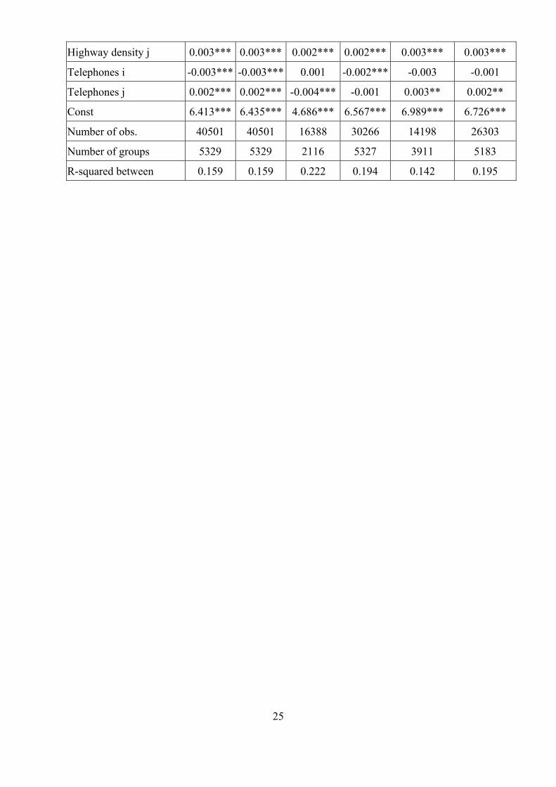
3.3 Results The results of fixed effects GLS estimations (equation (1)) are reported in Table A4.

Hausman test is rejected at the 1% level in all specifications so that the random effect model

is not valid.

12

The first two columns present the results of the regressions for the whole sample. The first

regression includes only income while the second one includes both income and squared

income. The other four are run for various subsamples to check robustness of the results. The

number of observations varies from 14 to 40 thousands. All results for indicators of economic

performance (income, unemployment and poverty) are significant and robust.

Economic performance and labor market conditions measured by the purchasing power of

average income and unemployment rate are significant both in host and source regions.

Outmigration rises with higher unemployment rate and inmigration grows with lower

unemployment rate. Coefficients show, that if the unemployment rate in a region increases by

1 per cent, ceterus paribus, then 0.7 per cent more people leave this region and at the same

time 1 per cent less people come.

Economic performance also matters: on average, higher real income attracts migrants and

reduces outflows of migrants. The most interesting results are the ones related to the non-

linear effect of income presented in the second column. The greater is the income in the host

region, the stronger the marginal effect – the coefficient at the squared income at the host

region is positive. This may be explained by a non-trivial fixed cost of moving – if income

differential is too small, only a few people are willing to move, but once the income

differential covers the fixed costs, more people respond to gross returns to mobility.

The effect of income in the source region on migration is negative on average, but its

magnitude is significantly weaker for poorer regions. Indeed, the coefficient at income is

–0.081 while the coefficient at the squared income is negative and equals –0.044 (both

coefficients are significant at 5 per cent level). The marginal effect of income on mobility is

therefore – 0.081 – 2*0.044*(income – 1.18). Hence, an increase in income increases

outgoing mobility for incomes below certain threshold level and decreases it otherwise. This

result is similar to what Banerjee and Kanbur (1981) have found for inter-regional rural-

urban migration in Indian states. As discussed above, this result is consistent with the

liquidity constraint hypothesis.

To find the threshold level of income at which the liquidity constraints become less important

than the effect of returns to mobility, one should calculate the peak of the estimated quadratic

function: 0.5*(-0.081±0.014)/(0.044±0.018) +1.18=0.26±3. This estimate is too crude, so we

have also used an alternative approach. Instead of including squared income, we ran the

regression for various subsamples of poorest regions. It turned out that for the the subsample

13

of 35% or less observations with lowest income, higher income increases outgoing mobility

(reported in the column (5) of Table A4). The 35% percentile corresponds to incomes below

2.98 consumer baskets (log income below 1.04). Once we take the 40%, the coefficient at

income becomes insignificant. For the sample of the richest 65% and for the whole sample it

is negative and significant (see columns (1) and (6) of Table A4). The result is striking:

roughly one third of Russian regions are locked in the poverty traps. In 1999, 28% Russian

population resided in regions with income below the threshold level. In Figure 1, these

regions are marked with bars; the height of the bar shows the gap between the regional

income and the threshold level.

The share of privately owned apartments is positively correlated with inmigration and

negatively (except for the regression for the European part) with outmigration. This may

reflect the higher utility of being able to own a home. On the other hand, this may be related

to the progress of reforms in the region (assuming that the mobile part of population prefers

economic reforms). This result is at odds with the evidence from cross-section data in Brown

(1997), where apartment privatization increases outgoing mobility (which may be explained

by the need to sell an apartment to finance the move). This suggests that cross-section

analysis may sometimes be misleading.

The next set of results deals with different measures of public goods provision within a

region. According to the famous Tiebout hypothesis, people ‘vote with their feet’ for better

provision of local public goods. Ceteris paribus, agents prefer a region with better public

goods provision. This hypothesis appears to hold for public healthcare and infrastructure.

Greater per capita number of buses, hospital beds, road density, telephones decrease

population outflow. At the same time more doctors, hospital beds, roads, and telephones

stimulate migration inflow. The magnitude of these effects is substantial: one standard

deviation change in each variable results in a 5 to 10 per cent change in the migration rates.

The counter-intuitive results are those for the railroads density: the density of railroads

positively influences outmigration and decreases inmigration; one has to keep in mind,

however, that the change in the railroads in 1992-99 was almost exclusively about closing the

old railroads rather than constructing new ones. The effect of crime rates on the inflows is

insignificant. Surprisingly, higher crime rates significantly reduce outflow; once we control

for poverty, however, the sign becomes intuitive (positive).

Table A4 does not present time dummies. These are shown in the Figure 2, along with the

overall intra-Russia migration rates in these years. Despite the remaining interregional gaps

14

in income and unemployment, migration has been declining over time. A possible

explanation is based on the existence of poverty traps. Apparently, those were both willing

and able to migrate, have migrated in the early years. The remaining potential migrants may

be too poor to afford the move.

To check whether the results are robust, we ran the regression for several subsamples

(columns 3 to 6 in Table A4).6 The third regression presents results for the subsample of the

48 regions that belong to the European part of Russia. The fourth regression includes poverty

level. Unfortunately, this reduces the sample to only 6 years (the poverty data have been

collected since 1994). All regressions show that results are quite robust but there are some

minor changes. The fifth column shows results for migration from the 35% observations with

lowest incomes, while the sixth regression is run for the rest of sample. These regressions

confirm the importance of liquidity constraints. For the poor regions, the effect of income is

positive, significant and quite large: a 10% raise in real income increases outgoing migration

by 1.6%

It is interesting to test what part of variation is explained by the current economic variables

and public goods provision. In turned out that both fixed effects and time-varying indicators

explain substantial shares of the variation in migration. In the regressions with five thousand

fixed effects and seven time dummies only, the R2-within was 0.13, compared with 0.16

when another 24 time-varying variables are included.

Besides estimating the determinants of migration controlling for region-to-region fixed

effects, we have also estimated the between-effects model (equation (2)). Results of the six

regressions are reported in Table A5 in Appendix.

All regressions show that population in both sending and receiving regions is a significantly

positive determinant of migration flows. As expected, larger regions send and attract more

migrants. Elasticities of migration with respect to the population of both sending and

receiving regions are close to 1 in almost all specifications.

Elasticity of migration with respect to distance is negative and significant, with its absolute

value being approximately equal to 1. This suggests that at least to a certain extent, low

mobility in Russia is related to huge distances. Indeed, as a thought experiment, let us reduce

6 We have also tried different specifications for the whole sample. We have estimated a dynamic migration model using Arellano-Bond linear, dynamic panel data estimator for autoregressive model in first differences assuming endogeneity of some explanatory variables. Results are similar. Table A6 presents the Poisson estimations which are also similar except for the regression for the European part of Russia.

15

Russia’s territory by 50 times to make it comparable with Japan (with population lower by 15

per cent), Norway or Finland. Then internal mobility of Russians will increase sevenfold and

exceed Japanese mobility by the factor of 2, Norwegian mobility by 50%, and will be higher

than the mobility in Finland (which is among the highest in EU). At the same time, this

exercise may be misleading: other countries of similar size (US, Canada and Australia) do

have much higher internal migration rates. Also, USSR had the same geographical problems

and still had high migration rates.

Other geographical variables also play an important role. Migrants tend to move to regions

with access to sea and largest rivers. Availability of port provides the region with 15-20 per

cent additional migrants. This may be related to better opportunities of entrepreneurship.

Educational level significantly increases both incoming and outgoing flows, but outflow is

more sensitive than inflow. An additional year of education increases outmigration by 40 per

cent.

The last set of results describes the impact of the progress of reforms in a region. Small

business privatization approximated by the share of privatized firms in trade and services

seems to favor both migration inflows and outflows. On the other hand, government subsidies

per 100 rubles of agricultural production reduce both inflows and outflows significantly.

These results suggest that state intervention cannot attract labor force but can make people in

those regions less mobile.

How do out coefficients compare to estimates for other countries? We are aware of five

similar studies, most of which are using Poisson model or extended Negative Binomial model

accounting for overdispersion, or extra-Poisson variation: Shen (1999) for China, Congdon

(1988) for Greater London, Boyle and Halfacree (1995) for England and Wales, Fik and

Mulligan (1998) for the US, and Devillanova and Carcia-Fontes (1998) for Spain.

Unfortunately, population size and distance are the only variables common to all of these

studies. Our estimates of elasticities of migration with respect to population (from 0.9 to 1.6

in the core models) are above the ones from these studies, 0.4-0.8 for Spain provinces and

0.3-0.9 in China. Our result on distance elasticity (-0.9 in the core model) is very close to

distance elasticity of labor migration in US, (-0.8 -1.1) and slightly below that in Spain and

China, (-1.1). Some studies include income and unemployment, results being similar to ours.

In Spain, income in origin area has a negative effect on outmigration. Also, negative sign for

16

unemployment in destination is reported for London and positive impact of the ratio between

unemployment in origin to that in destination is found in Spain.

4 Concluding remarks The main goal of this paper is an empirical analysis of internal migration in Russia. We use a

panel dataset of gross migration flows between Russian regions. Our methodology allows

distinguishing the effect of current economic performance and public goods provision in the

regions from the long-term trends in migration due to inertia and Soviet-time legacies. The

empirical analysis shows that although overall internal migration is low in Russia, it does

depend on income per capita, unemployment rate, poverty and public goods provision in the

intuitive way, controlling for fixed effects (for each pair of host-source regions) and

macroeconomic shocks. This has important policy implications for Russia’s regional policy

and fiscal federalism. Indeed, our analysis suggest that there is Tiebout competition between

Russian regions. The impact of economic performance of the region on migration is not

trivial. Regional policies that improve living standards, create jobs and improve public goods

provision, do attract migrants. These effects are substantial relative to average migration rate.

Our empirical analysis shows that liquidity constraints are an important barrier to migration.

The population of the poorest regions cannot leave simply because they are unable to finance

the cost of moving. For these regions, income growth increases rather than decreases

outgoing migration. The financial constraints effectively attach the population to the region,

reducing outside options and wages. We estimate that a third of Russian population is locked

in such poverty traps.

We have also found that elasticity of migration to distance is as high as in other countries (i.e.

close to one), so the effect of the geography on the interregional labor reallocation should not

be underestimated.

Two caveats are due. First, we use official data that do not account for informal migration.

Informal migration is at least as high in Russia as the official one. What is more important, it

may be not proportional to official migration; e.g., the informal migration is higher in places

where one needs authorities’ permission to register. Hence the analysis of official migration

may be biased. Second, we study regional rather than individual data. This implicitly assumes

that migrants are representative of their region, which is unlikely. These two problems cannot

be resolved without migration data from a nationally representative survey of potential and

actual migrants that (to the best of our knowledge) does not exist.

17

In our future research, we are going to extend our analysis in several directions. First, to deal

with possible endogeneity problems, we will look for good instrumental variables. Another

extension is to carry out more accurate dynamic panel data analysis by running GMM system

estimation with joint weak endogeneity of some explanatory variables introduced by

Arrelano and Bond (1991). Third, we are going to break the region-to-region migration flows

into rural and urban categories and study the determinants of mobility to and from rural and

urban areas. Even in the developing countries, rural-urban migration accounts for only 30 per

cent of total migration (Lucas, 1997). One should expect that in Russia that is already an

industrialized country the urban-urban and urban-rural migration plays an important role,

especially given that our research shows that education and access to finance should make

urban population more mobile.

5 References Ahrend, R. (2000) “Speed of Reform, Initial Conditions, Political Orientation, or What?

Explaining Russian Regions' Economic Performance,” RECEP Working Paper No.

2000/2, Moscow.

Andrienko, Yu. (2001). “V poiskah ob’yasneniya rosta prestupnosti v Rossii v perekhodniy

period: Ekonomitcheskiy i kriminometritcheskiy podkhodi“ [Explaining Crime Growth in

Russia during Transition: Economic and Criminometric Approach], Economic Journal of

the Higher School of Economics, No.2. [in Russian]

Arellano, M., and S. R. Bond (1991) “Some Tests of Specification for Panel Data: Monte

Carlo Evidence and an Application to Employment Equations”, Review of Economic

Studies, 58, pp. 277-297.

Banerjee, B., and S. M. Ravi Kanbur (1981). “On the specification and estimation of macro

rural-urban migration functions: with application to Indian data”, Oxford Bulletin of

Economics and Statistics 43, pp. 7-29.

Besstremyannaya, G. (2001). “The Applicability of the Tiebout Hypothesis to Russian

Jurisdictions”, Master Thesis, New Economic School, Moscow.

Boeri, T., and C. J. Flinn (1999). “Returns to Mobility in the Transition to a Market

Economy”, Journal of Comparative Economics 27, pp. 4-32.

Boeri T., M. Burda, and J. Kollo (1996). “Mediating the Transition Labor Markets in Central

and Eastern Europe”, Economic Policy Intitiative, No.4, CEPR, London.

Boyle P.J., and K.H. Halfacree (1995). “Service Class Migration in England and Wales,

1980-1981: Identifying Gender-specific Mobility Patterns”, Regional Studies, 29 (1), pp.

43-57.

Brown, A.N. (1997) “The Economic Determinants of Internal Migration Flows in Russia

During Transition”, Department of Economics, Western Michigan University, Mimeo.

Brown, D., and J. Earle (2003) “Gross Job Flows in Russian Industry Before and After

Reforms: Has Destruction Become More Creative?”, Journal of Comparative Economics,

forthcoming.

Congdon, P. (1988). “Modelling Migration Flows between Areas: An Analysis for London

Using the Census and OPCS Longitudinal Study”, Regional Studies, 23 (2), pp. 87-103.

19

Expert Institute (2000).“Monotowns and town-shaping enterprises”, Expert Institute,

Moscow. [In Russian]

Devillanova, C., and W. Garcia-Fontes (1998). “Migration across Spanish Provinces:

Evidence from the Social Security Records (1978-1992)”, Working Paper 319,

University Pompeu Fabra, Barselona.

Faggio, G., and J. Konings (1999). “Gross Job Flows and Firm Growth in the Transition

Countries: Evidence Using Firm Level Data on Five Countries”, CEPR Discussion Paper

No. 2261, London.

Fik T.J., and G.F. Mulligan (1998) “Functional form and spatial interaction models”,

Environment and Planning A, 30, pp. 1497-1507.

Filer, R.K., T.Gylfason, Š. Jurajda, and J. Mitchell (2001). “Markets and growth in the post-

communist world”, mimeo, Global Development Network, Washington, DC.

Friebel, G., and S. Guriev (2000) “Why Russian workers do not move: attachment of workers

through in-kind payments” CEPR Discussion Paper No. 3268, London.

Gang, I. N., and R.C. Stuart (1999). “Mobility where mobility is illegal: Internal migration

and city growth in the Soviet Union”, Journal of Population Economics, 12, pp. 117-134.

Gerber, T. P. (2000) “Regional Miration Dynamics in Russia Since the Collapse of

Communism”, University of Arizona, Mimeo.

Ghatak S., P. Levine, and P.S. Wheatly (1996). “Migration Theories and Evidence: An

Assessment”, Journal of Economic Surveys, 10 (2).

Goskomstat (2000) “Regioni Rossii: statistitcheskiy sbornik” [Russian Regions: Statistical

Yearbook], State Statistics Committee, Moscow, Russia. [in Russian]

Greenwood, M. J. (1997). “Internal Migration in Developed Countries” in Handbook of

Population and Family Economics, eds. M. R. Rozenzweig and O. Stark, Elsevier

Science.

Heleniak, T. (1997). “Internal Migration in Russia During the Economic Transition”, Post-

Soviet Geography and Economics, 38 (2), pp. 81-104.

20

Heleniak, T. (1999) “Out-Migration and De-Population of the Russian North During the

1990-es”, Post-Soviet Geography and Economics, 40 (3), pp.155-205.

Korel L., and I. Korel (1999) “Migrations and Macroeconomic Processes in Post-socialist

Russia: Regional Aspect”, mimeo, Economic Education and Research Consortium,

Moscow.

Lucas R.E.B. (1997) “Internal Migration in Developing Countries” in Handbook of

Population and Family Economics, eds. M. R. Rozenzweig and O. Stark, Elsevier

Science.

Regent, T. M. (1999). “Migratsiya v Rossii: Problemy Gosudarstvennogo Upravleniya”,

(Migration in Russia: the Problems of Government Management), Moscow: ISESP

Publishers. [In Russian]

Shelley, L. (1982) “Soviet Population Migration and Its Impact on Crime”, Canadian

Slavonic Papers, XIII (1), pp. 77-87.

Shen, J. (1999)“Modelling regional migration in China: estimation and decomposition”,

Environment and Planning A, 31, pp. 1223-1238.

Svejnar J. “Labor Markets in the Transitional Central and East European Economies” in

Handbook of Labor Economics, Volume 3, eds. O. Ashenfelter and D. Card, Elsevier

Science B. V., 1999.

World Bank, “The Russian Federation After the 1998 Crisis: Towards “Win-win” Strategies

for Growth and Social Protection”, May 2001.

Zayonchkovskaya, Zh. A. (1994) “Migration of population and labor market in Russia”,

Institute for Economic Forecasting, Moscow, 1994. 66 P. [in Russian]

Zayonchkovskaya, Zh. A. ed. (2001) “Labor Migration in Russia and Abroad”, Minfederatsii,

Moscow. [in Russian]

Zohoori N., T. Mroz, B. Popkin, E. Glinskaya, S. Lokshin, D. Mancini, P. Kozyreva,

M.Kosolapov, and M. Swafford (1998) “Monitoring the Economic Transition in the

Russian Federation and its Implications for the Demographic Crisis – the Russian

Longitudinal Monitoring Survey”, World Development, 26, pp. 1977-93.

20

Appendix. Table A1. Migration in Russia, percent of mid-year present-in-area population 1990 1991 1992 1993 1994 1995 1996 1997 1998 1999 Total arrivals 4.1 3.5 3.0 2.7 2.9 2.7 2.4 2.2 2.1 1.9 Out of which From Russia 2.9 2.5 2.2 2.0 2.0 2.1 2.0 1.8 1.8 1.7 Out of which Same region 1.2 1.0 1.0 1.1 1.1 1.0 1.0 0.9 Other regions 1.0 0.9 1.0 1.0 0.9 0.8 0.8 0.8 Other countries 0.7 0.5 0.7 0.7 0.8 0.6 0.4 0.4 0.3 0.3 N/A 0.5 0.5 0.1 0.1 0.1 0.0 0.0 0.0 0.0 0.0 Total departures 3.6 3.2 2.7 2.4 2.3 2.3 2.1 2.0 1.9 1.8 Out of which Within Russia 2.7 2.3 2.1 2.0 2.0 2.1 1.9 1.8 1.7 1.7 Out of which Same region 1.2 1.0 1.0 1.1 1.1 1.0 1.0 0.9 Other regions 0.9 1.0 1.0 0.9 0.8 0.8 0.8 0.7 Other countries 0.5 0.5 0.5 0.3 0.2 0.2 0.2 0.2 0.1 0.2 N/A 0.4 0.4 0.1 0.1 0.1 0.0 0.0 0.0 0.0 0.0

21

Table A2. Segmentation of the labor market and real income per capita Unemployment rate (ILO definition)

Year Obs Mean Std. Dev. Min Max 1990 77 4.1 1.8 0.7 11.5 1991 77 4.1 1.8 0.7 11.5 1992 77 5.2 1.6 2.0 14.5 1993 77 6.1 1.9 3.3 17.5 1994 77 8.6 2.3 4.6 18.0 1995 79 11.0 5.6 5.4 43.1 1996 79 11.1 4.8 5.5 32.2 1997 79 13.8 6.6 4.8 58.2 1998 79 15.3 6.3 4.7 51.1 1999 79 15.4 6.4 5.6 51.8

Real income per capita: Number of 25-product baskets that the regional monthly income can buy.

Year Obs Mean Std. Dev. Min Max 1990 76 8.4 3.2 4.0 25.6 1991 76 7.7 3.0 3.6 23.3 1992 76 3.6 1.2 1.7 10.0 1993 76 3.5 1.0 2.1 7.7 1994 76 2.9 0.9 1.7 7.6 1995 79 3.1 1.4 0.9 12.5 1996 79 3.5 1.9 1.3 16.2 1997 79 4.3 1.8 1.8 15.4 1998 79 3.0 1.4 1.3 12.5 1999 77 3.5 1.7 1.5 14.3

22

Table A3. Descriptive statistics of the variables. Var Definition Obs Mean Std. Dev. Min Max

Migration (log) Number of people migrated from one region to another 40501 4.5 1.5 -0.7 11.2

Life expectancy Life expectancy from birth, years 40501 65.9 2.1 55.3 72.3

Conflict General socio-political conflict indicator 40501 8.5 6.3 0.2 46.6

Income (log) December average income in 25-good-basket 40501 1.2 0.3 0.2 2.8

Unemployment Unemployment rate, per cent (ILO methodology) 40501 10.5 4.9 2.8 31.2

Poverty Share of population with income below subsistence level 30266 30.8 13.1 11.5 88.8

Share of men Share of men as of beginning of 1991 40501 47.3 1.4 45.1 50.4

Share of young Share of young people from 0 to 15 years of age as of beginning of 1991

40501 24.7 3.2 19.4 35.5

Share of old Share of old people, men from 60 and women from 55 years of age as of beginning of 1991

40501 18.7 4.4 7.1 25.7

Apartment privatization

Share of privately owned apartment 40501 35.2 14.9 1.0 73.0

Homicides Homicide rate per 1.000 population 40501 0.19 0.07 0.04 0.42

Buses Number of buses per 100.000 population 40501 83 19 32 156

Doctors Number of doctors per 1.000 population 40501 9 8 1 73

Hospital beds Hospital beds per 1.000 population 40501 1.3 0.1 0.8 1.9

Railroad density Railroad density km per 10.000 km^2 40501 170 121 0.5 586

Highway density Highway density km per 1.000 km^2 40501 108 75 1.5 327

Telephones Number of telephones per 100 households 40501 35 11 18 105

Population (log) Population as of beginning of 1990, thousands 39069 7 1 5 9

Distance (log) Distance between two regions, km 39069 7.6 1.1 3.2 9.5

Education Average years of education of population above 15 years of age 39069 9.3 0.3 8.7 10.1

23

ELF Ethno-linguistic fractionalization 39069 0.3 0.2 0.1 0.8

Large cities Share of population residing in cities with more 500.000 population

39069 0.1 0.2 0.0 0.6

Rural population Share of rural population 39069 0.3 0.1 0.1 0.6 Resource potential Resource potential index 39069 1.0 0.5 0.4 2.7

Temperature in January

Average temperature in January, degrees centigrade 39069 -13 7 -37 -1

Temperature in July

Average temperature in July, degrees centigrade 39069 18 2 12 25

Dummy for port Dummy for regions with major ports 39069 0.2 0.4 0 1

Subsidies to agriculture

Budget subsidies per 100 rubles of agricultural production as of 1995

39069 10 5 1 29

Small privatization

Share of privatized businesses in trade, catering and household services as of 1996

39069 82 33 20 306

Price regulation Proportion of goods and services with regulated prices as of 1996 39069 16 9 3 69

24

Table A4. Regression results: GLS fixed effect regressions for migration. Migration and income are in logs, including squared log of income. Therefore, the respective coefficients are elasticities of migration with respect to income. The squared income is adjusted for 1.18 (the mean income for the entire sample) to reduce correlation between income and squared income. Significance levels: *** - 1%, ** - 5%, * - 10%. Index ‘i’ denotes source region and ‘j’ denotes destination.

Variable Core 92-99

Main 92-99

Main for European Part 92-99

Main with poverty 94-99

Core for poorest 35%

92-99

Core for richest 65%

92-99 Unemployment i 0.007*** 0.007*** 0.008*** 0.005*** 0.012*** 0.006***

Unemployment j -0.010*** -0.011*** -0.014*** -0.006*** -0.008*** -0.012***

Income i -0.080*** -0.081*** -0.037** 0.046** 0.161*** -0.163***

Income j -0.001 -0.0001 0.057*** -0.144*** -0.039 0.018

(Income – 1.18)2 i -0.044** -0.017 -0.049***

(Income – 1.18)2 j 0.063*** 0.067** 0.065***

Poverty i 0.0004

Poverty j -0.002***

Life expectancy i -0.020*** -0.020*** -0.019*** -0.029*** -0.0016 -0.024***

Life expectancy j -0.0012 -0.0019 0.020*** -0.003 -0.012** 0.007*

Socio-political conflict i -0.001 -0.0006 0.002** -0.0004 0.005*** -0.003***

Socio-political conflict j -0.002*** -0.002*** -0.001 -0.004*** -0.004*** -0.002***

Apartment privatization i -0.003*** -0.003*** 0.004*** -0.002** -0.008*** 0.0002

Apartment privatization j 0.003*** 0.003*** 0.004*** 0.003*** 0.002* 0.004***

Homicides i -0.385*** -0.373*** 0.129 0.363*** -0.441** -0.493***

Homicides j 0.014 -0.003 0.067 -0.056 -0.327 0.174

Buses i -0.003*** -0.003*** -0.003*** -0.002*** -0.002*** -0.003***

Buses j -0.0002 -0.0003 -0.001* 0.0003 -0.0007 0.000

Doctors i 0.015*** 0.015*** 0.020*** 0.014*** 0.027** 0.015***

Doctors j 0.009** 0.008* -0.026*** 0.047*** 0.024*** -0.005

Hospital beds i -0.34*** -0.342*** -0.160** -0.104* -0.0733 -0.565***

Hospital beds j 0.235*** 0.239*** 0.222*** 0.123** 0.131 0.311***

Railroad density i 0.0004* 0.0004* 0.001*** 0.001*** -0.01*** 0.001***

Railroad density j -0.002*** -0.002*** -0.002*** -0.002*** -0.002*** -0.002***

Highway density i -0.002*** -0.002*** -0.001*** -0.001* -0.003*** -0.001***

25

Highway density j 0.003*** 0.003*** 0.002*** 0.002*** 0.003*** 0.003***

Telephones i -0.003*** -0.003*** 0.001 -0.002*** -0.003 -0.001

Telephones j 0.002*** 0.002*** -0.004*** -0.001 0.003** 0.002**

Const 6.413*** 6.435*** 4.686*** 6.567*** 6.989*** 6.726***

Number of obs. 40501 40501 16388 30266 14198 26303

Number of groups 5329 5329 2116 5327 3911 5183

R-squared between 0.159 0.159 0.222 0.194 0.142 0.195

26

Table A5. Regression results: GLS between-effects regressions for migration.

Variable Core 92-99

Main 92-99

Main for European Part 92-99

Main with poverty 94-99

Core for poorest 35%

92-99

Core for richest 65%

92-99 Distance -0.922*** -0.922*** -1.38*** -0.921*** -0.916*** -0.909***

Education i 0.432*** 0.45*** -0.363 0.41*** 0.367*** 0.719***

Education j 0.133 0.113 -0.277 0.214** 0.393*** 0.198**

Unemployment i 0.052*** 0.057*** 0.088*** 0.041*** 0.068*** 0.03***

Unemployment j -0.005 -0.010 0.069*** -0.011 -0.005 -0.008

Income i -0.105 0.008 -0.276 0.619*** 0.853*** -0.518***

Income j 0.152 0.033 0.372* 0.749*** 0.102 0.076

(Income-1.18)2 i -0.272* -2.42*** -0.597***

(Income-1.18)2 j 0.288** -1.25* -0.1058

Poverty i 0.014***

Poverty j 0.016***

Life expectancy i -0.18*** -0.172*** 0.144*** -0.141*** -0.023 -0.141***

Life expectancy j -0.133*** -0.142*** -0.025 -0.125*** -0.048*** -0.085***

Socio-political conflict i 0.008** 0.004 0.014 0.005 -0.013*** 0.003

Socio-political conflict j -0.009** -0.005 -0.022** -0.005 -0.004 -0.013***

Log population i 1.609*** 1.608*** 0.40** 1.418*** 1.159*** 1.483***

Log population j 0.923*** 0.924*** 0.817*** 0.968*** 0.774*** 0.785***

Initial share of men i 0.173*** 0.174*** 0.802*** 0.22*** 0.42*** 0.273***

Initial share of men j 0.116*** 0.115*** 0.548*** 0.141*** 0.192*** 0.16***

Initial share of young i -0.106*** -0.107*** -0.03 -0.117*** -0.17*** -0.072***

Initial share of young j -0.056*** -0.056*** 0.076** -0.065*** -0.036* -0.026

Initial share of old i -0.105*** -0.106*** 0.203*** -0.09*** -0.074*** -0.052**

Initial share of old j -0.048** -0.046** 0.164*** -0.038* -0.004 -0.016

Apartment privatization i 0.013*** 0.013*** 0.014*** 0.012*** 0.001 0.01***

Apartment privatization j 0.015*** 0.014*** 0.011** 0.012*** 0.008*** 0.01***

Homicides i -2.319*** -2.191*** 4.453*** -1.628*** -0.648 -1.721***

Homicides j -2.008*** -2.144*** 0.815 -1.662*** -1.005*** -1.622***

Buses i 0.003*** 0.003*** -0.001 0.002* 0 0.003***

Buses j -0.0004 -0.001 -0.003** -0.0006 -0.001 -0.0004

Doctors i -0.085*** -0.082*** 0.0144 -0.067*** -0.026*** -0.063***

Doctors j -0.004 -0.007 0.002 -0.009 0.006 0.01

27

Hospital beds i 0.362*** 0.391*** -2.438*** 0.25* -0.734*** 0.441***

Hospital beds j -0.367*** -0.396*** -2.081*** -0.380*** -0.254* -0.359***

Railroad density i 0.0004* 0.0004* -0.0002 0.0003 -0.0003 0.000

Railroad density j 0.001*** 0.001*** -0.0005 0.001** 0.001*** 0.001***

Highway density i 0.0004 0.0004 0.0003 0.001* -0.0001 0.0006

Highway density j 0.0006 0.0007 0.003*** 0.001*** 0.0001 0.0004

Telephones i -0.020*** -0.022*** 0.009** -0.019*** -0.021*** -0.018***

Telephones j -0.018*** -0.015*** 0.006 -0.014*** -0.018*** -0.017*** Ethno-linguistic fractionalization i -0.532*** -0.494*** 1.214*** -0.492*** -0.193 -0.561***

Ethno-linguistic fractionalization j -0.129 -0.168 0.597* -0.290* -0.33** -0.281*

Big cities i 0.38*** 0.319*** -0.668*** 0.301*** -0.218 0.289***

Big cities j 0.096 0.161 -0.353* 0.098 0.065 0.087

Rural i 1.904*** 2.034*** -2.986*** 1.734*** 1.351*** 1.855***

Rural j 1.038*** 0.902*** -2.241*** 0.778*** 0.766*** 0.791***

Resource potential i 0.192*** 0.169*** 0.358*** 0.245*** 0.101 0.1**

Resource potential j 0.235*** 0.259*** 0.328*** 0.236*** 0.29*** 0.281***

Temperature in January i -0.034*** -0.034*** -0.06*** -0.032*** -0.038*** -0.031***

Temperature in January j -0.024*** -0.024*** -0.046*** -0.017*** -0.029*** -0.024***

Temperature in July i -0.043*** -0.047*** -0.099*** -0.039*** -0.061*** -0.049***

Temperature in July j -0.036*** -0.031*** -0.046** -0.026** -0.037*** -0.048***

Dummy for port i 0.147*** 0.142*** 0.286*** 0.118*** 0.128** -0.0335

Dummy for port j 0.193*** 0.198*** 0.222*** 0.145*** 0.162*** 0.185***

Subsidies to agriculture i -0.001 -0.002 -0.022*** -0.001 -0.011** -0.009***

Subsidies to agriculture j -0.002 -0.002 -0.016*** 0.0004 -0.012*** -0.003

Small privatization i 0.001** 0.001** 0.003 0.001*** 0.002*** 0.001

Small privatization j 0.001*** 0.001** -0.0003 0.001*** 0.001** 0.001**

Price regulation i 0.0002 -0.0001 -0.002 -0.001 -0.005*** -0.002

Price regulation j -0.001 -0.0004 0.0004 -0.001 -0.003** -0.002

Const 1.5987 1.6418 -64.114*** -6.931 -26.068*** -14.172***

Number of obs. 39069 39069 15488 28850 13942 25127

Number of groups 5041 5041 1936 5039 3811 4899

R-squared within 0.765 0.766 0.78 0.756 0.766 0.754

28

Table A6. Regression results: Poisson fixed effect regressions for migration.

Variable Core 92-99

Main 92-99

Main for European Part 92-99

Main with poverty 94-99

Core for poorest 35%

92-99

Core for richest 65%

92-99 Unemployment i 0.014*** 0.014*** 0.017*** 0.011*** 0.007*** 0.016***

Unemployment j -0.009*** -0.009*** -0.011*** -0.006*** -0.003*** -0.012***

Income i -0.040*** -0.036*** -0.058*** 0.041*** 0.057*** -0.063***

Income j 0.091*** 0.085*** 0.073*** 0.021*** 0.018*** 0.084***

(Income 1.18)2 i -0.024*** 0.028*** -0.0313***

(Income 1.18)2 j 0.063*** -0.009* 0.097***

Poverty i 0.0007***

Poverty j -0.001***

Life expectancy i -0.028*** -0.027*** -0.039*** -0.032*** -0.032*** -0.028***

Life expectancy j 0.019*** 0.018*** 0.035*** 0.013*** -0,002 0.03***

Socio-political conflict i -0.002*** -0.002*** 0,0001 0.0004*** -0.002*** -0.002***

Socio-political conflict j 0.001*** 0.001*** -0.002*** -0.001*** -0.002*** 0.003***

Apartment privatization i 0.002*** 0.002*** 0.002*** 0.002*** 0.001*** 0.002***

Apartment privatization j 0.001*** 0.001*** 0.001*** 0.002*** -0.001*** 0.002***

Homicides i -0.027* -0.012 0.015 0.412*** 0.532*** -0.336***

Homicides j -0,013 -0.044*** 0.12*** -0.397*** -0.868*** 0.366***

Buses i -0.001*** -0.001*** -0.001*** -0.001*** -0.002*** -0.001***

Buses j 0.0006*** 0.0004*** 0.001*** 0.0002*** -0,0001 0.0006***

Doctors i 0.014*** 0.014*** 0.009*** 0.006*** 0.038*** 0.012***

Doctors j 0.005*** 0.004*** -0.008*** 0.019*** 0.005*** 0.002***

Hospital beds i -0.079*** -0.082*** -0.028** -0.043*** -0.167*** -0.031***

Hospital beds j 0.155*** 0.16*** 0.033** 0.209*** 0.265*** 0.112***

Railroad density i 0.0003*** 0.0002*** 0.000 0.001*** 0.003*** 0.0003***

Railroad density j -0.001*** -0.001*** -0.002*** -0.001*** 0.002*** -0.002***

Highway density i -0.002*** -0.002*** -0.001*** 0.0001* -0.001*** -0.002***

Highway density j 0.002*** 0.002*** 0.002*** 0.0003*** 0.003*** 0.002***

Telephones i 0.002*** 0.002*** 0.003*** 0.002*** -0.001*** 0.003***

Telephones j -0.003*** -0.003*** -0.008*** -0.006*** -0.004*** -0.001***

Number of obs. 40496 40496 16388 30123 13588 25906

Number of groups 5328 5328 2116 5184 3305 4786

29

Figure 1. Net migration, total for 1990-99 as % of 1990 population (color) and gap between regional income and the threshold level (bar).

-56 to -6-6 to 00 to 33 to 44 to 66 to 42

% below threshold:

2 27 51

Figure 2. Evolution of migration over time: the intra-Russia migration rates in 1992-99 and time dummies in the core regression. Since the regression is run for the log migration, the graph presents exp(year dummies).

0,0

0,5

1,0

1,5

2,0

2,5

1990 1992 1994 1996 1998 20000,00,20,40,60,81,01,2

Migration in Russia, % population, left scaleexp(year dummies), right scale