DETERMINANTS OF HOUSEHOLD ACCESS TO ANDPARTICIPATION IN FORMAL AND INFORMAL CREDIT

MARKETS IN MALAWI

Aliou Diagne

FCND DP No. FCND DP No. 6767

FCND DISCUSSION PAPER NO. 67

Food Consumption and Nutrition Division

International Food Policy Research Institute2033 K Street, N.W.

Washington, D.C. 20006 U.S.A.(202) 862–5600

Fax: (202) 467–4439

May 1999

FCND Discussion Papers contain preliminary material and research results, and are circulated prior to a fullpeer review in order to stimulate discussion and critical comment. It is expected that most Discussion Paperswill eventually be published in some other form, and that their content may also be revised.

ABSTRACT

The paper uses the concept of credit limit to analyze the determinants of household

access to and participation in informal and formal credit markets in Malawi. Households

are found to be credit constrained, on average, both in the formal and informal sectors;

they borrow, on average, less than half of any increase in their credit lines. Furthermore,

they are not discouraged in their participation and borrowing decisions by further

increases in the formal interest rate and/or the transaction costs associated with getting

formal credit. This suggests that getting access to credit is much more important than its

cost for these households. Hence, credit policies should focus on making access easier

rather than providing credit with subsidized interest rates.

The composition of household assets is found to be much more important as a

determinant of household access to formal credit than the total value of household assets

or landholding size. In particular, a higher share of land and livestock in the total value of

household assets is negatively correlated with access to formal credit. However, land

remains a significant determinant of access to informal credit. Therefore, poor

households whose assets consist mostly of land and livestock but who want to diversify

into nonfarm income generation activities may be constrained by lack of capital. As

informal loans are usually too small to help poor households start a viable nonfarm

iii

business, these households may be forced to rely on farming as the sole source of income,

despite its unreliability because of the frequency of drought in Malawi.

Finally, formal and informal credit are found to be imperfect substitutes. In

particular, formal credit, whenever available, reduces but does not completely eliminate

informal borrowing. This suggests that the two forms of credit fulfill different functions

in the household’s intertemporal transfer of resources.

CONTENTS

Acknowledgments . . . . . . . . . . . . . . . . . . . . . . . . . . . . . . . . . . . . . . . . . . . . . . . . . . . . vi

1. Introduction . . . . . . . . . . . . . . . . . . . . . . . . . . . . . . . . . . . . . . . . . . . . . . . . . . . . . . . 1

2. Measurement and Determinants of Access to Credit . . . . . . . . . . . . . . . . . . . . . . . . . 4

Analyzing Access to Credit with the Credit Limit Variable . . . . . . . . . . . . . . . . . . 5Access to Credit and Participation in Credit Programs . . . . . . . . . . . . . . . . . . . . . 7“Expectations,” Observability of the Credit Limit, and the Demand for Credit . . . 8

3. Specification of the Empirical Model . . . . . . . . . . . . . . . . . . . . . . . . . . . . . . . . . . . 11

Identification of the Model . . . . . . . . . . . . . . . . . . . . . . . . . . . . . . . . . . . . . . . . . 13Sampling and Estimation Methodologies . . . . . . . . . . . . . . . . . . . . . . . . . . . . . . 14

4. Empirical Results . . . . . . . . . . . . . . . . . . . . . . . . . . . . . . . . . . . . . . . . . . . . . . . . . . 20

Structure of the Formal and Informal Credit Markets in Malawi . . . . . . . . . . . . . 21Determinants of Participation in and Access to Credit Markets in Malawi . . . . . . 23

Determinants of Participation in Credit Programs . . . . . . . . . . . . . . . . . . . 24Determinants of the Extent of Household Access to Credit . . . . . . . . . . . . 26Determinants of Demands for Formal and Informal Loans . . . . . . . . . . . . 28

5. Conclusion . . . . . . . . . . . . . . . . . . . . . . . . . . . . . . . . . . . . . . . . . . . . . . . . . . . . . . . 32

Appendix 1: Partial Effect b of When Only Expected b Is Observed . . . . . . . . . . 36max max

Appendix 2: Correcting for the Effects of Choice-based Sampling . . . . . . . . . . . . . . . 38

Appendix 3: Data and Empirical Results . . . . . . . . . . . . . . . . . . . . . . . . . . . . . . . . . . . 44

References . . . . . . . . . . . . . . . . . . . . . . . . . . . . . . . . . . . . . . . . . . . . . . . . . . . . . . . . . . 57

TABLES

1 Formal and informal credit limits in Malawi (October 1993 toDecember 1995) . . . . . . . . . . . . . . . . . . . . . . . . . . . . . . . . . . . . . . . . . . . . . . . . 45

v

2 Formal and informal loan sizes in Malawi (October 1993 toDecember 1995) . . . . . . . . . . . . . . . . . . . . . . . . . . . . . . . . . . . . . . . . . . . . . . . . 46

3 Formal and informal unused credit lines in Malawi (October 1993-December 1995) . . . . . . . . . . . . . . . . . . . . . . . . . . . . . . . . . . . . . . . . . . . . . . . . 47

4 Definition and summary statistics of variables used in the model . . . . . . . . . . . . . 48

5 Probability choice model parameters . . . . . . . . . . . . . . . . . . . . . . . . . . . . . . . . . 50

6 Predicted conditional probability choices (standard errors in parentheses) . . . . . . 51

7 Matrix of partial changes of probability choices with respect to changes inselected independent variables . . . . . . . . . . . . . . . . . . . . . . . . . . . . . . . . . . . . . . 52

8 Formal credit limit equation (FLOANMAX): Matrix of direct and indirectpartial effects of selected variables . . . . . . . . . . . . . . . . . . . . . . . . . . . . . . . . . . . 53

9 Informal credit limit equation (ILOANMAX): Estimated coefficients ofselected variables (partial effects) . . . . . . . . . . . . . . . . . . . . . . . . . . . . . . . . . . . . 54

10 Formal credit demand equation (FLOANVAL): Matrix of direct and indirectpartial effects of selected variables . . . . . . . . . . . . . . . . . . . . . . . . . . . . . . . . . . . 55

11 Informal credit demand equation (ILOANVAL): Matrix of direct andindirect partial effects of selected variables . . . . . . . . . . . . . . . . . . . . . . . . . . . . . 56

FIGURES

1 Distribution of formal and informal credit limits in Malawi (October 1993 toDecember 1995): Box plot diagrams . . . . . . . . . . . . . . . . . . . . . . . . . . . . . . . . . 45

2 Distribution of formal and informal loan sizes in Malawi (October 1993 toDecember 1995): Box plot diagrams . . . . . . . . . . . . . . . . . . . . . . . . . . . . . . . . . 46

3 Distribution of unused formal and informal credit lines in Malawi (October1993 to December 1995): Box plot diagrams . . . . . . . . . . . . . . . . . . . . . . . . . . . 47

vi

ACKNOWLEDGMENTS

This paper has benefitted from the comments of Manfred Zeller, Andrew Foster,

Alain de Janvry, Manohar Sharma, Lawrence Haddad, Hanan Jacoby, Soren Hauge, John

Strauss, and seminar participants at the International Food Policy Research Institute

(IFPRI) and the 1998 annual meeting of the American Economic Association. Financial

support from the Rockefeller Foundation and from the German Agency for Technical

Cooperation (GTZ), the United States Agency for International Development (USAID),

and the United Nations Children's Fund (UNICEF) offices in Malawi is gratefully

acknowledged.

Aliou DiagneVisiting Research FellowInternational Food Policy Research Institute

1. INTRODUCTION

It has been a long-held belief among policymakers that poor households in

developing countries lack access to adequate financial services for efficient intertemporal

transfers of resources and risk coping, and that without well-functioning financial

markets, these households do not have much prospect for increasing in any significant

and sustainable way their productivity and living standards. Because of these reasons,

and the fact that traditional commercial banks typically have no interest in lending to poor

rural households due to their lack of viable collateral and the high transaction costs

associated with the small loans that suit them, most developing-country governments and

donors have set up during the past three decades credit programs aimed at improving

rural household access to formal credit. The vast majority of these credit programs,

especially the so-called “agricultural development banks,” which provided credit at

subsidized interest rates, have failed to achieve their objectives both to serve the rural

poor and be sustainable credit institutions (Adams, Graham, and von Pischke 1984;

Braverman and Guasch 1986; Adams and Vogel 1986).

Both in response to these failures and in recognition of the critical role that credit

can play in alleviating rural poverty in a sustainable way, innovative credit delivery

systems are being promoted throughout the developing world as a more efficient way of

improving rural households’ access to formal credit with no or minimal government

2

involvement. The failure of government-supported financial institutions throughout the

developing world has also convinced many researchers of the need for a better

understanding of how poor households in less-developed countries, often living in highly

risky environments, insure against risk and conduct their intertemporal trade in the

absence of well-functioning financial markets (Deaton 1989; Coate and Ravallion 1993;

Townsend 1994; Udry 1994, 1995; Fafchamps 1992).

Several studies conducted in the past two decades have substantially increased

economists' understanding of the workings of informal financial institutions in

developing countries (see, for examples, the surveys by Besley 1995, Alderman and

Paxson 1992, and Gersovitz 1988). The studies have revealed the complex strategies

used by poor households in developing countries to increase their productive capacity,

share risks, and smooth consumption over the life cycle. These strategies generally work

through self-enforcing informal contracts among friends, neighbors, and members of the

extended family, and are arranged within networks of informal institutions of diverse

natures (Fafchamps 1992; Coate and Ravallion 1993; Udry 1994; Lund and Fafchamps

1997; Kochar 1997). These nonmarket informal institutions, the economic rationales of

which have long eluded the attention of researchers and policymakers, have often been

found to outperform the financial institutions governments have set up to serve the rural

population. One hypothesis that is often advanced by researchers and policymakers to

explain this phenomenon is that government- and nongovernment organization (NGO)-

supported credit programs often crowd out the financial services offered by these

3

informal financial institutions. Hence, understanding how nonmarket informal

institutions serve the financial need of households and interact with the formal credit

institutions set up by governments and NGOs is important. Such understanding is

valuable for sustainable and market-oriented financial institutions that would expand and

complement the services offered by the existing informal credit market rather than

substitute for them.

This paper analyzes what determines the extent of household access to informal

and formal credit markets in Malawi and how severe are household credit constraints.

The paper also analyzes household demand for formal and informal credits and provides

empirical evidence on the substitutability between formal and informal credits in Malawi.

The analysis is based on a data set collected in a three-round survey of 404 households in

45 villages and five districts of Malawi conducted in 1995 and 1996. To satisfactorily

analyze the determinants of both access to credit and participation in formal credit

programs, the paper makes the distinction between access to credit (formal or informal)

and participation (in formal credit programs or in the informal credit market). A

household has access to a particular source of credit if it is able to borrow from that

source, although for some reasons it may choose not to borrow. This paper measures the

extent of access to credit as the maximum amount a household can borrow (credit limit).

The paper is organized as follows: Section 2 presents the methodology of the paper

and discusses the conceptual differences between the various credit-related concepts used.

Section 3 briefly describes the structure of the formal and informal credit markets in

4

Malawi and the data used in this paper. Section 4 presents the results of the econometric

analysis of the determinants of the extent of households’ access to informal and formal

credit markets, as well as households’ demand for formal and informal credits. Section 5

concludes the paper with some final remarks on the policy implications of the findings of

the paper.

2. MEASUREMENT AND DETERMINANTS OF ACCESS TO CREDIT

There are presently two methodologies for measuring household access to credit

and credit constraints in the literature. The first method infers the presence of credit

constraints from violations of the assumptions of the life-cycle/permanent-income

hypothesis. More precisely, the method uses household consumption and income data to

look for a significant dependence (or “excess sensitivity”) of consumption on transitory

income. Empirical evidence of significant dependence is taken as an indication of

borrowing or liquidity constraint (see, for examples, the recent surveys by Browning and

Lusardi [1996] and Besley [1995]). The second method directly uses information on

households’ participation and experiences in the credit market to classify them as credit

constrained or not. The classification is then used in reduced form regression equations

to analyze the determinants of a household being credit constrained (see Jappelli 1990;

Feder et al. 1990; Zeller 1994; Barham and Boucher 1994). The shortcomings of these

two approaches are reviewed in Zeller et al. (1996 and 1997) and Diagne, Zeller, and

Sharma (1997). The next section develops a methodology based on the credit limit

5

concept, which allows a more satisfactory analysis of the determinants of the extent of a

household’s access to credits and its demand for formal and informal credits.

ANALYZING ACCESS TO CREDIT WITH THE CREDIT LIMIT VARIABLE

In general, lenders are constrained by factors outside their control on the maximum

amount they can possibly lend to any potential borrower. Consequently, any borrower,

however creditworthy, faces a limit on the overall amount s/he can borrow from any

given source of credit, regardless of the interest rate s/he is willing to pay and/or collateral

he is willing to put up to back the loan. Furthermore, due to the possibility of default and

lack of effective contract enforcement mechanisms, lenders have the incentive to further

restrict the supply of credit, even if they have more than enough to meet a given demand

and the borrower is willing to pay a high enough interest rate (Avery 1981; Stiglitz and

Weiss 1981). Therefore, from the borrower’s view, the relevant limit on supply is not the

maximum the lender is able to lend, but rather the maximum the lender is willing to lend.

The latter perceived maximum limit or credit limit that cannot be exceeded when

borrowing, regardless of how much interest one is willing to pay, is the focus of the

methodology used in this paper for quantifying the extent of household access to credit.

To motivate the reduced form equations estimated in the empirical section of the

paper, a conceptual framework focusing explicitly on the credit limit variable is

summarized (see Diagne, Zeller, and Sharma 1997 for more details). The conceptual

framework basically follows from a contract-theoretic view of loan transactions (see

bmax

bmax

b amax

b amax

bmax

b (

6

Freixas and Rochet 1997, for example). The framework is based essentially on the fact

that the credit limit variable, , facing a potential borrower, and the amount the

potential lender wants to be repaid, are the variables that lenders can choose. On the

other hand, the optimal amount, b , to be borrowed within the range set by the lender*

remains the sole choice of the borrower, who also chooses ex-post (i.e., once the loan is

disbursed) whether and when to pay back the loan.

The lender’s optimal choice of , which is interpreted here as the supply for

credit, is a function of the maximum s/he is able to lend, . It is also a function of the

lender’s subjective assessment of the likelihood of default and of other borrowers’

characteristics. However, this function is not a supply-for-credit function in the

traditional meaning of the term, where, under the assumption of price-taking behavior, the

supply-for-credit function represents the schedule of what the lender is willing to lend as

the market interest rate varies. This traditional supply function for credit is not defined in

this context, in which the lender him or herself chooses the interest rate. Similarly, the

optimal interest rate, r, chosen by the lender is a function of , the lender’s subjective

assessment of the likelihood of default and other borrowers’ characteristics. The reader is

referred to Avery (1981) and Stiglitz and Weiss (1981), respectively, for an empirical and

formal analysis of how the lender’s assessment of the likelihood of default affects the

optimal choice of both and r. On the other hand, the function defining the

borrower’s optimal choice of loan size, , is a demand-for-credit function in the

traditional meaning of the term (i.e., the schedule of what the borrower is willing to

b ( bmax

bmax

bmax

bmax

7

borrow when the interest rate varies). The fact that is a function of in addition to

being a function of the interest rate is a mere reflection of the borrowing constraint and

the imperfect substitutability of the different sources of loans. However, because of

imperfections in the enforcement of the loan contract and the resulting adverse selection,

the demand for credit need not be a downward-sloping function of the interest rate.

Hence, as pointed out by Stiglitz and Weiss (1981), lenders cannot use the interest rate as

a way of rationing credit.

ACCESS TO CREDIT AND PARTICIPATION IN CREDIT PROGRAMS

Access to formal credit is often confused with participation in formal credit

programs. Indeed, the two concepts are often used interchangeably in many credit

studies. The crucial difference between the two concepts lies in the fact that participation

in a credit program is something that households choose to do freely, while access to a

credit program entails constraints placed on households (availability and eligibility

criteria of credit programs, for example). In other words, participation is more of a

demand-side issue related to the potential borrower’s choice of the optimal loan size, b ,*

while access is more of a supply-side issue related to the potential lender’s choice of the

maximum credit limit, . The lack of access to credit for a given source of credit can

be defined as when the maximum credit limit, , for that source of credit is zero. That

is, one has access to a certain type of credit when the maximum credit limit, , for that

bmax

bmax

bmax

bmax

8

credit type is strictly positive; and one improves someone’s access to that type of credit by

increasing for that credit.

“EXPECTATIONS,” OBSERVABILITY OF THE CREDIT LIMIT, AND THEDEMAND FOR CREDIT

The observations above suggest that the maximum credit limit a borrower faces

depends on both the lender and the borrower’s characteristics and actions. But it depends

also on random events that affect the fortune of lenders and other potential borrowers

(who may compete with the borrower for the same possible credit). For example, one can

expect the occurrence of drought in a rural agriculture-based economy to reduce the

supply of informal credit, while also increasing the number of people looking for loans.

Hence, the maximum credit limit, , facing a potential borrower is a random variable

whose values are determined by events of which only some are under the borrower’s

control; others are under the lender’s control and still others outside the control of both.

The fact that depends on random events also implies that its realized value at

the times when borrowing actually takes place cannot be known exactly in advance by

either the lender or the borrower. The fact that it cannot be known in advance by the

borrower is clear, since the realized value ultimately will be the result of the lender’s

choice (although, as explained above, the borrower can influence that choice to some

extent). The borrower can only form “expectations” about the likely value of at the

time of actual borrowing. But formal lenders usually provide enough information about

their loan policy (eligibility criteria, types of project funded, collateral and down-payment

bmax

bmax

bmax

bmax

bmax

bmax

bmax

9

requirements, and so on) to enable potential borrowers to have reasonably accurate

“expectations” about their from each source of formal credit. In most NGO and

government-supported credit programs, lenders even set and announce fixed credit limits

for all potential borrowers.

Furthermore, at the time of borrowing, it is only the lender who observes the

realized value of (which the lender himself/herself determines), and may or may not

have the opportunity to reveal it to the borrower. For example, if the borrower’s realized

optimal choice of loan size is strictly positive but strictly less than the realized value of

, then the lender may never have the chance to tell the borrower his or her actual

realized choice of . Clearly, if at a particular time, a borrower does not ask for a loan

from a given source of credit, that borrower will never learn, even in retrospect, about his

or her realized from that source of credit at that time (there may be exceptions in the

cases of NGO- and government-supported credit programs that set and announce fixed

credit limits for all potential borrowers). However, the potential borrower will always

have “expectations” on what would have been the likely value of . Furthermore, it is

precisely the borrower’s prior “expectations” about the likely value of and its

variability that influence his or her behavior and make him or her decide whether or not

to seek a loan from that particular source of credit. For example, in the direct method of

detecting credit constraints discussed above, the classification of borrowers usually

includes a class of “discouraged borrowers” (see Jappelli 1990, for example). These

“discouraged borrowers” did not seek any loan because either they expected to face zero

bmax

bmax

bmax

bmax

bmax

bmax

bmax

bmax bmax

bmax

bmax

10

or very low , or they expected a relative high cost (including transaction costs) for

getting loans. The “discouraged borrowers” may have been wrong in their expectations

and could perhaps obtain worthwhile loans at reasonable costs. But, whether they are

wrong or right, at the end, it is the “expectations” about their that have determined

their behavior, not the realized values of their , which will remain unknown to them.

Even when borrowers seek loans from a given source of credit, the realized value of the

optimal loan size is largely determined by the borrowers’ “expectations” about their

(especially if the borrowers have reasonably accurate information that allows them to

predict accurately the location of ).

The arguments above imply that in the analysis of the demand for credit, the

borrower’s “expectations” about are much more important in determining the

actually demanded amounts of credit than the realized values of . However, from a

policy point of view, what is of interest a priori is not the borrower’s response to changes

in his or her “expectations” about , but his or her response to “change” in itself,

because this is the variable under the lender’s control and it determines access to credit.

In the empirical evidence presented in the next section, the borrower’s expected

from different sources of credit is analyzed. The survey from which the data are drawn

did not collect the realized values of , which only lenders could provide with some

reasonable accuracy. The survey focused on the demand side of the credit market, and for

a relative large survey, it is not feasible to interview the lender for each loan transaction.

bmax b (

bmax b (

bmax

bmax bmax

bmax bmax

bmax

11

Moreover, borrowers may not be willing to identify their informal lenders or may refuse

to be interviewed if they know that the latter are going to be interviewed as well.

However, with an econometric analysis, it is possible to estimate and evaluate the

impact of on and other household choice or outcome variables, based solely on

expected . For this to be possible, it is necessary to assume that the realized and

other household choice or outcome variables depend only on expected and not on

higher moments of and its realized values. This restriction is plausible if does

not vary much (so that its variance and higher centered moments are close to zero) and

the borrower has reliable information that allows him or her to predict the location of

with reasonable accuracy (so that the realized value of will have little influence

on realized optimal choices). Under this restriction, the impacts of on household

choice and outcome variables can be assessed by exploiting the proprieties of the

mathematical expectation operator, which, as usual, is identified with the borrower’s

“expectation process” (see Appendix 1).

3. SPECIFICATION OF THE EMPIRICAL MODEL

The reduced form equations for the determination of the maximum credit limits

and the demands for credit presented below can be rationalized by a household utility

maximization model in which the contractual relationships between the household and its

lenders and the (imperfect) substitutability between formal and informal credit are

bmax

b Fmax' "1x1 % $F

1z F1 % gF ,

b Imax' "2x2 % $I

1zI1 % gI,

b F ' "3x3 % $F2z F

2 % *Fr % (F1b F

max% (I1b

Imax% u F ,

b I' "4x4 % $I2z

I2 % *Ir % (F

2b Fmax% (I

2bImax% u I,

b Fmax b I

max b F b I

z F

z I

12

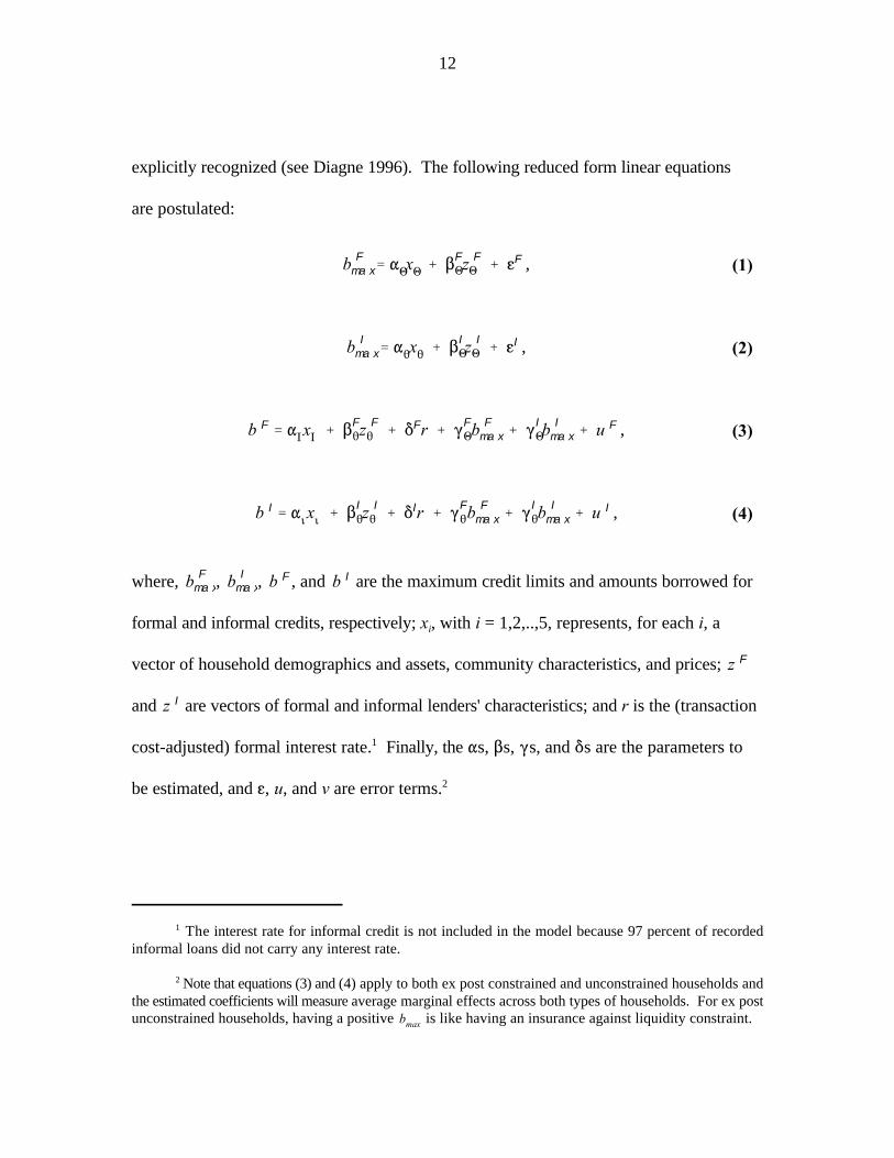
The interest rate for informal credit is not included in the model because 97 percent of recorded1

informal loans did not carry any interest rate.

Note that equations (3) and (4) apply to both ex post constrained and unconstrained households and2

the estimated coefficients will measure average marginal effects across both types of households. For ex postunconstrained households, having a positive is like having an insurance against liquidity constraint.

(1)

(2)

(3)

(4)

explicitly recognized (see Diagne 1996). The following reduced form linear equations

are postulated:

where, , , , and are the maximum credit limits and amounts borrowed for

formal and informal credits, respectively; x , with i = 1,2,..,5, represents, for each i, ai

vector of household demographics and assets, community characteristics, and prices;

and are vectors of formal and informal lenders' characteristics; and r is the (transaction

cost-adjusted) formal interest rate. Finally, the "s, $s, (s, and *s are the parameters to1

be estimated, and g, u, and v are error terms. 2

13

IDENTIFICATION OF THE MODEL

Equations (1) to (4) constitute a recursive system of simultaneous equations with

the exogenous variables constituted by the household demographics and assets,

community characteristics, and lenders’ characteristics appearing in all equations. Hence,

exclusion restrictions on these variables are needed for the system to be identified. The

simultaneity of the maximum credit limit variables (which are choice variables for

lenders, not borrowers) result from the fact that they are likely to be correlated with

unobservable household characteristics (the likelihood of defaulting, for example)

absorbed into the error terms, u and v. It is clear that any household demographic,

community characteristics, and prices observed by the econometrician can reasonably be

expected to be observable by informal lenders. The same can be said for formal lenders,

especially those that use the group-based lending technology. In addition, these

observables are likely to determine both lenders’ choices of credit limits and the

borrowers’ choices of loan sizes. Therefore, as argued by Udry (1995), one should not

expect to be able to find exclusion restrictions on these sets of variables to identify

equations (3) and (4).

The main argument used for identifying equations (3) and (4) is that not all the

lender’s characteristics variables enter directly into the determination of the amount

borrowed. That is, some of the lender’s characteristics influence the amounts borrowed

only through the effects they have in determining how much the lender is willing to lend.

For informal credit, the information collected on the lender’s characteristics are relative

bmax

14

All the other potential variables (such as source of program funding, whether the program is for3

agricultural inputs or for nonfarm income, etc.) turned out to be perfectly correlated with the program dummies.

One can conceive of circumstances in which the lender’s identity influences directly the size of the4

loan sought by a borrower. For example, borrowers may be willing to borrow more from lenders with laxcredit recovery systems compared to those who punish default harshly, even if the maximum credit limits fromboth sources are the same. This possibility is ruled out for the purpose of identifying the model.

Only the characteristics of those lenders whose loan transactions were recorded are used as5

instruments. Unfortunately, we did not collect the characteristics of lenders for households that were notinvolved in any loan transaction (although their were collected). The information could have beencollected but we became aware of the problem too late in the survey. The characteristics of formal andinformal lenders used in the estimation are all in the form of dummy variables, which were set to zero forhouseholds not involved in any loan transaction.

wealth compared to the borrower, professional occupation, relation to the borrower, place

of residence, and whether he or she is a member of a credit program. It is argued that all

these characteristics influence the amounts borrowed only through the informal

maximum credit limit. For formal credit, the only available information on the lender’s

characteristics are the program dummy variables. It is argued here that these program3

dummies, which stand for the formal lenders’ identities and other unobserved specific

attributes, influence the amounts borrowed only through the formal maximum credit

limit. Prices and selected community characteristics variables were also used as4, 5

additional instruments (see Tables 8 and 9 in Appendix 3 for details).

SAMPLING AND ESTIMATION METHODOLOGIES

The data used in the analysis come from a year-long three-round survey (February

1995 - December 1995) of 404 households in 45 villages in five districts of Malawi

where the four microcredit programs studied were operating. The four microcredit

15

programs are Malawi Rural Finance Company (MRFC, a state-owned and nationwide

agricultural credit program), Promotion of Micro-Enterprises for Rural Women

(PMERW, a microcredit program for nonfarm income generation activities supported by

the German Agency for Technical Cooperation [GTZ]), the Malawi Mudzi Fund (MMF,

an IFAD-funded program modeled on the Grameen Bank and now incorporated into

MRFC), and the Malawi Union of Savings and Credit Cooperatives (MUSCCO, a union

of locally based saving and credit unions). All the programs are based on group lending

except MUSCCO.

If the sample were drawn randomly, then given the above identifying restrictions,

the system can be estimated straightforwardly using standard simultaneous equation

estimation methods. However, despite the fact that there are numerous credit programs

operating in various part of Malawi, credit program participation is still a rare reality

found only in a few villages. Out of 4,700 households enumerated in the 45 villages

covered in the village census, only 12 percent were current members of a credit program.

Moreover, the 12 percent figure significantly overstates the likelihood of credit program

membership in Malawi because it represents the percentage of membership in villages

that are actually hosting the four credit programs studied. The majority of villages in

Malawi do not host any credit program. This fact alone ruled out at the outset straight

random sampling at any geographical level above the village level. Since it was

necessary to include enough credit program participants for the study, the only feasible

alternative was to stratify along the program membership status variable with random

E(yi|xi) '"xi%jJ&1

j'1$jwji

i'1,...,n ,

16

(5)

selection within each strata. About half of the sample were participants of the four credit

programs. The second half of the sample were equally divided between past participants

(mostly from a failed government credit program), and households that never participated

in any formal credit program. The reader is referred to Diagne, Zeller, and Mataya (1996)

for details on the survey and data collection methodology.

Under the circumstances stated above, not only is the chosen method of choice-

based sampling more cost-efficient than straight random sampling, but it also yields,

provided the appropriate estimation methods are used, estimates with better statistical

properties than those obtained under straight random sampling (Manski and McFadden

1981; Cosslett 1981 and 1993; Amemiya 1985). Appendix 1 shows that the choice-based

sampling correction required when estimating the system (equations [1]-[4]) involves

only the equations where the program dummies appear as regressors. Moreover, the

correction consists merely of replacing the program dummies by the corresponding

choice-based-corrected conditional probability choices. The choice-based corrected

equations have the following form:

where y and x are generic dependent variable and regressor, respectively, and

Q(j)/H(j)

wj/

H(j)Q(j)

p(j|x)

jJ

j'1

H(j)Q(j)

p(j|x)

j'1,...,J

p(j|x)

H(j)/nj/n

Q(j)/Nj/N

p(j|x)

p(j|x)

17

The ratio is the sample analogue of the Manski-Lerman weight used in the weighted6

maximum likelihood procedure to get consistent estimates under choice-based sampling (see Manski andMcFadden 1981, or Amemiya 1985, chapter 9).

(6)

are the choice-based-corrected conditional probability choices, while " and $ are thej

parameters to be estimated. The indices j = 1,...,J are the mutually exclusive J program

choices defining the strata, and j designates the strata of the i household; is theith

population conditional choice probability that program j is chosen, given x.

and are the respective sampling and population ratios, with n (resp N ) beingj j

the size of the sample (resp population) strata defined by program j, and n and N being

the total sample and population sizes, respectively. Note that the calculation of the partial

effects of any variable in an equation corrected for choice-based sampling has to take into

account the changes in the w if that variable appears also as a regressor in the estimationj

of the .

A two-stage estimation method similar to Heckman’s two-step procedure for Tobit

models is used to estimate equation (5). In the first stage, the Manski-Lerman weighted

maximum likelihood estimator is used to consistently estimate the conditional probability

choices and construct the w . In the second stage, the estimated w are used inj j6

18

equation (5) to estimate each resulting equation with an Ordinary Least Squares (OLS) or

Two-Stage Least Squares (TSLS) procedure, depending on the equation.

A four-alternative, two-level nested multinomial logit model is used to estimate the

population conditional choice probabilities (see Appendix 2 for details). However, the

model allows the vector of parameters to be different across the four alternative choices

(Judge et al. 1985; Maddala 1983; Schmidt and Strauss 1975). In the first level of the

nesting, the choice is between participation and nonparticipation in a credit program. In

the second level, which is reached only if participation is the chosen alternative, the

choice is between (1) joining and remaining a member of MRFC, (2) joining and

remaining a member of the second program, and (3) joining either MRFC or the second

program and then dropping out of the program (i.e., being a past member). The

classification defined by the four mutually exclusive alternative choices corresponds

exactly to the stratification used in selecting the households. In each village, there are, at

most, two credit programs operating: MRFC and one of the other three programs, which,

as choice variable, is generically called PROG2 in the estimated model. However, the

program dummy variables (Mudzi, MUSCCO, and PMERW) were used as alternative-

specific regressors instead of the generic label. As usual in a multinomial discrete choice

model, these dummy alternative-specific variables control for unobserved attributes

specific to each alternative; they can explain why a household prefers one alternative over

another (see, for example, Manski and McFadden 1981; Cosslett 1981, 1993). In fact, for

PMERW, its two sister programs (designated here as PMERW1 and PMERW2) are

19

PMERW1 is a revolving fund targeted to very poor women, while PMERW2 operates through one7

of the main commercial banks in Malawi as a loan guarantee scheme. PMERW2 members are either“graduates” of PMERW1 or successful, but not very wealthy, businesswomen living in the areas covered bythe program.

All the partial effects are calculated for each households before taking weighted averages across8

households. This is preferable to evaluating partial effects at the means because of the nonlinearities in theprobability choices (all estimations and computations were performed with GAUSS).

differentiated because of their different attributes and target groups. Therefore, the7

partial effects for all the program dummies are estimated for both the conditional

probability choices and the equations including the three choice-based-corrected

conditional probability choices for MRFC, PROG2, and Past members (these constitute

the w above and are called WMRFC, WPROG2, and WPAST in the tables in Appendix 3j

that report the results of the estimation). 8

Finally, the estimation procedure follows McFadden’s (1981) sequential maximum

likelihood estimation for nested multinomial logit models. Because of the sequential

nature of McFadden’s procedure, the usual maximum likelihood standard errors are not

valid. Therefore, the Bootstrap method (Effron and Tibshirani 1993; Jeong and Maddala

1993), implemented by replicating (with replacement) exactly the sampling procedure

used to select the households, is used to calculate standard errors for all the estimated

conditional probability choice parameters and the ones for the subsequently estimated

simultaneous equations system. To account for the possibility of the instruments being

only weakly correlated with the endogenous variables, the relevant F statistics and

exogeneity and overidentification test statistics for each equation were computed

following Staiger and Stock (1997).

20

4. EMPIRICAL RESULTS

The information collected in the survey includes household demographics, land

tenure, agricultural production, livestock ownership, asset ownerships and transactions,

food and nonfood consumption, credit, savings and gift transactions, wages, self-

employment income and time allocation, and anthropometric status of preschoolers and

their mothers. The agricultural data cover the 1993/94 and 1994/95 seasons. Because the

methodology used to measure access to credit is based on the maximum credit limit, few

details will be given on the way the variable was collected in the survey.

The questionnaire on credit and savings was administered to all adult household

members (over 17 years old) in the sample. In each round, respondents were asked the

maximum amount they could borrow during the recall period from both informal and

formal sources of credit. If the respondent was involved in a loan transaction as a

borrower, the question was asked for each loan transaction (both for granted and rejected

loan demands). In this case, the maximum credit limit is referring to the time of

borrowing and to the lender involved in that particular loan transaction. If the respondent

did not ask for any loan, the question was asked separately for formal and informal

sources of credit with no reference to particular formal or informal lenders. Respondents

who were granted loans were also asked the same general question (i.e., with no reference

to particular formal or informal lenders) in a way that elicited the maximum credit limit

they would face if they wanted more loans, not just from the same lender, but from the

same sector of the credit market (formal or informal) from which they have borrowed.

Q(j)/H(j)

21

Given the central importance of the credit limit variable for the methodology of the study, several9

other control questions were used to verify the consistency of the answers given by the respondents to thisquestion. Such control questions included household program membership status; whether respondents weregiven a lesser amount if they received a loan, how much did they ask for; whether they did ask for a loan andwere rejected; and why they did not ask for any (or more) loans. In addition, the enumerators were instructedto use other control questions not included in the questionnaires whenever there seemed to be inconsistenciesin the respondent’s answers.

To correct for the over sampling of credit program participants, the summary statistics in the tables10

have been weighted using the strata population and sample ratios ( ); corrected with weightsconstructed using the district-level 1987 population census data.

The exchange rate is 1 US dollar for 15 Malawi kwacha (Mk).11

Consequently, for both formal and informal credit, the maximum formal and informal

credit limits of each adult household member were obtained in each round, even if the

member was not involved in any loan transaction.9

STRUCTURE OF THE FORMAL AND INFORMAL CREDIT MARKETS INMALAWI

Appendix 3, Table 1 presents the average maximum informal and formal credit

limits from October 1993 to December 1995 for the whole population and for formal

sector borrowers only. In particular, the table shows that the average maximum formal10

and informal credit limits for the population as a whole are 167 and 99 Malawi kwacha

(Mk), respectively. The corresponding figures for formal-sector borrowers were 67511

and 90 Mk, respectively. To put these figures in perspective, Malawi’s 1995 per capita

GNP was US$170 (i.e., 2,550 Mk) and the average per capita 1995 income in the sample

was 1,190 Mk. The box plot diagrams of the distributions presented in Appendix 3,

Figure 1 give a better picture of the extent of access to credit in Malawi. The figure

22

shows that the median formal and informal credit limits in the population as a whole are,

respectively, zero and 40 Mk. Fifty percent of the population can borrow, at most, 100

Mk (less than $10) from either sector of the credit market. One notes that formal-sector

borrowers have higher median formal credit limits (375 Mk) but lower median informal

credit limits (20 Mk). This is likely to reflect the fact that two of the credit programs

studied are targeted to poor women who might have been excluded from the few existing

sources of informal credit because of their socioeconomic situation (see Appendix 3,

Figure 1).

With regard to household participation in formal credit programs and the informal

credit market, there were 372 loans granted during the survey, 41 percent of which were

from the formal sector of the credit market. These included all formal loans taken since

membership in the credit programs began (1992 only for the old government credit

program) and relatively large-sized informal loans (more than 100 Mk) taken since

October 1994 and up through December 20, 1995. For informal loans of less than 15 Mk

and for those between 15 and 100 Mk, the recall period were 8 weeks and 3 months,

respectively. There were 100 demands for loans rejected, 56 percent of which were

rejected by informal lenders. In total, 71 percent of adult individuals in the sample did

not ask for any loan during the three rounds of the survey. The most common reason for

not asking for formal or informal loans was dislike of or no need for borrowing (48

percent and 27 percent for informal and formal, respectively). Informal loans were

mostly between friends and relatives (93 percent). The majority of them did not have any

23

For comparison, 2,233 informal and 338 formal loans were recorded in Bangladesh in a similar IFPRI12

survey in 1994 involving 350 households (Zeller, Sharma, and Ahmed 1995). In another similar IFPRI surveyof 189 households in Madagascar in 1991, there were 1,375 and 245 informal and formal loans, respectively(Zeller et al. 1993).

due date (57 percent). Virtually all informal loans were interest-free loans (98 percent)

with an average size of 76 Mk for the period October 1993 to December 1995. In

contrast, formal loans carried an average annual interest rate of 39 percent and their

average size was 530 Mk. These figures show that the credit market in Malawi is not as

active as in other Asian and African countries.12

DETERMINANTS OF PARTICIPATION IN AND ACCESS TO CREDIT MARKETSIN MALAWI

The system of equations (1)-(4) was estimated using the two-stage methodology

presented in the previous section. The estimation results for the conditional probability

and for the credit limits and loan demands equations are presented in Appendix 3, Tables

5–11. The relevant F statistics and exogeneity and overidentification test statistics are

also presented for each equation. In particular, one notes the high F statistics for the joint

significance of the lenders’ characteristics (the program dummies) in the formal credit

limit equation (F = 50.41). On the other hand, the F statistics for the joint3,1505

significance of the informal lenders’ characteristics in the informal credit limit equation is

relatively low F = 3.88). This indicates that the informal lenders’ characteristics may7,1505

introduce biases in the TSLS estimates of the credit demand equations due to their weak

correlations with the informal credit limit (Staiger and Stock 1997). Furthermore, for

24

When the instruments are weakly correlated with the endogenous regressors, Staiger and Stock13

(1997) recommend using the Durbin and Basmann tests when testing the exogeneity and overidentificationrestrictions, respectively. The Basmann test uses the Limited Information Maximum Likelihood (LIML)estimates.

There was not much difference between the TSLS and OLS estimates, however.14

both the formal and informal credit demand equations, the Wu-Hausman and Durbin tests

fail to reject the null hypothesis of exogeneity of the presumed endogenous variables.

The overidentifying restrictions are also rejected by the Basmann test. Under these13

conditions, it is more appropriate to estimate the two credit demand equations by OLS.

Therefore, the results are reported as OLS.14

Determinants of Participation in Credit Programs

The parameter estimates of the conditional probability choice estimation are

presented in Appendix 3, Table 5, but will not be discussed. Instead, the more readily

interpretable partial changes in the probability choices are discussed in the following

paragraph. The predicted conditional probability choices are presented in Appendix 3,

Table 6, with their bootstrap standard errors. The table shows that there is a 62 percent

chance that a household will participate in a credit program. Once a household has

decided to participate, there is a 36 percent chance that it will join and stay with MRFC, a

28 percent chance that it will join and stay with one of the other four programs, and a 36

percent chance that it will join one of the five programs and then drop out (either

voluntarily or by defaulting).

25

Appendix 3, Table 7 presents the absolute partial changes in the four probability

choices after marginal changes in the independent variables. First, controlling for all

other factors, the unobserved specific program attributes picked up by the program

dummies have statistically significant influences on the average household’s decision to

participate. The attributes of MRFC have, however, the greatest influence (+11 percent

absolute increase in the probability of participating compared to 8 percent for PMERW

and Mudzi Fund, and 4 percent for MUSCCO). Once the decision to participate has been

made, the unobserved specific program attributes have statistically significant effects on

the choice of joining a specific program or leaving after joining. Everything else being

equal, MRFC’s unobserved specific attributes increase the probability of joining and

staying with MRFC by 26 percent in absolute terms and reduce the probabilities of

joining a second program and leaving MRFC by 11 percent and 15 percent in absolute

terms, respectively. The corresponding figures for the second program choice are

generally lower. For example, PMERW’s attributes, which have the strongest effects,

increase the probability of joining and staying with the second program (instead of

MRFC) by 20 percent in absolute terms, and reduce (in absolute terms) the probabilities

of joining MRFC by 10 percent and leaving the second program by 10 percent. The

opposite directions of these effects are reflections of the mutual exclusivity of the three

choices.

The other key variables that have statistically significant effects on program

membership decisions with expected signs are (1) having had any membership

26

application rejected (DMEMREJH), which decreases the probability of participating

(perhaps because rejected households become discouraged to apply again); (2) knowledge

of the existence of a credit club (DKNOWCLB), which increases the probabilities of

participating and joining MRFC and decreases the probability of being a past member;

(3) share of cultivable land out of total household land (AGLPAREA), which increases

the probability of participating; (4) share of value of land out of total household assets

(LDPASSTH), which increases the probability of joining the second program; (5) being a

male-headed household (MALEHEAD), which increases the probability of joining

MRFC but decreases the probabilities of joining the second program and being a past

member (this is not surprising because female-headed households are more likely to be

landless and therefore would prefer joining credit programs that lend for nonfarm

businesses rather than MRFC, which gives seasonal agricultural loans only). Finally, one

notes that both the household adult population size (POPADL15) and dependency ratio

(DEPRATIO) decrease the probability of participating, while the household adult

population size decreases the probability of joining MRFC but increases the probabilities

of joining the second program and being a past member.

Determinants of the Extent of Household Access to Credit

Appendix 3, Tables 8 and 9 present the results of the determinants of the extent of

household access to formal and informal credits as measured by household credit limits in

each market. First, one notes that, as expected, all five credit programs have contributed

27

statistically significantly to the access to formal credit by their member households. The

differences compared to noncurrent members range from as low as 20 Mk per capita per

season for MRFC to as high as 57 Mk per capita per season for PMERW1. Furthermore,

credit program members (NGOLEND) contribute significantly to the accessibility of

informal credit to other households. Also, the extent of household access to formal and

informal credits was significantly higher before October 1994 (see variable DP9495). For

formal credit, this reflects partly the longer recall period for loans before October 1994

and the fact that MRFC started operating only in October 1994, following the collapse of

the previous state-owned agricultural credit program.

Second, household total value of assets (TASSETVH) has no significant effects on

access to both formal and informal credits, whereas landholding size (LANDAREH) has

a positive but statistically significant effect only on access to informal credit. Although

not significant at the 5 percent level (a t-value of 1.8), the share of cultivable land in total

household land has a positive effect on access to formal credit. This positive effect can

be attributed to the fact that seasonal agricultural loans come as input packages

corresponding to farmers’ acreage. On the other hand, the marginal effects of the share of

the value of land in the total value of household assets is negative and statistically

significant for both access to formal and informal credits. The share of livestock in the

total value of household assets also has a negative and statistically significant effect on

access to informal credit. Hence, overall, these results suggest that the composition of

household assets is much more important in determining household access to formal

28

In particular, most of the PMERW credit groups are located around small rural towns or around so15

called “rural growth centers.”

credit in Malawi than the overall value of the assets. In particular, except for seasonal

agriculture loans, formal lenders are willing to lend less to households whose assets

consist mostly of land and livestock. However, landholding size remains a significant

determinant of access to informal credit.

The other demographic variables that have statistically significant effects on the

extent of access to formal credit are household adult population size and dependency

ratio, DEPRATIO (-); the number of wholesale buyers coming to the village, NWLSBUY

(+); distance to the home of the field credit officer, DISTFA (-); distance to the trading

center, DISTTCEN (-); and distance to the post office, DISTPO (+). Except for the

distance to the post office, the coefficients of these community “infrastructure” variables

have the expected signs. Indeed, for logistical and economic reasons, one should expect

the credit programs to tend to locate in trading centers and be willing to lend more to

households from villages with higher levels of economic activity. Finally, as the15

regression results show, gender, education, and occupation have no significant effect on

access to both formal and informal credits.

Determinants of Demands for Formal and Informal Loans

The estimation results for the determinants of the demand for formal and informal

loans are reported in Appendix 3, Tables 10 and 11. From Table 10, the average

29

marginal propensity to borrow out of every additional Mk of formal credit made available

(FLOANMAX) is estimated to be 0.49 Mk. It is statistically significantly different from

both zero and 1 (at the 5 percent level). Since the coefficient measures the marginal

increase in the average amount borrowed, it can be said that households are, on average,

constrained in their demand for formal credit and would borrow, on average, about half

the amount of any increase in their formal credit limits. As Appendix 3, Table 11 shows,

the same is also true for informal credit (ILOANMAX), but with much lower marginal

propensity to borrow (.07).

With regard to the substitutability between formal and informal sources of credit,

Appendix 3, Table 10 shows that the availability of informal credit (ILOANMAX) has a

negative but not statistically significant effect on the demand for formal credit. Similarly,

it can be seen in Table 11 that the availability of formal credit (FLOANMAX) induces a

very small and not statistically significant reduction in the demand for informal credit.

However, this marginal reduction in the demand for informal credit is much larger for

credit program members with statistically significant differences compared to noncurrent

members ranging from -0.07 Mk for MRFC to -0.19 Mk for PMERW1 per capita per

season. Therefore, at least for credit program members, formal and informal credits

appears to be substitutable.

The transaction cost-adjusted interest rate for formal credit (FAINRATT) does not

play any role in this substitutability between formal and informal sources of credit.

Therefore, at their present level of access to formal credit, households are not discouraged

30

The decrease in informal borrowing due to the existence of a due date is not statistically significant16

at the 5 percent level, but is at the 10 percent level (t-value = 1.86).

by further increases in interest rates. However, higher interest rates may not be in the

advantage of the lender because they increase the likelihood of default (Stiglitz and Weiss

1981). Some of the other terms of informal loan contracts seem to play a significant role

in this substitutability: When informal loans have due dates (IDUEDATE) or any

condition attached to them (INOCLCND), borrowing from formal sources is increased

significantly, while borrowing from the informal ones is decreased significantly. In16

contrast, formal loan due dates and conditions (FDUEDATE and FNOCLCND) and the

processing times of formal and informal loans (FWEEKDLY and IWEEKDLY) have no

statistically significant effect on the demands for formal and informal loans. Hence,

when deciding which source of loans to use when they are both available, borrowers seem

to care more about the “noncost attributes” of the informal loans they have access to and

less about the relative cost of the two types of loans.

One can note from the tables that increases in the price of maize (PVMAIZE) and

fertilizer (PCFERT95) increase significantly the demand for formal loans. On the other

hand, the producer price of tobacco (PPTOB95) and those for seed—hybrid maize

(PSHMZ95), local maize (PSLMZ95), and tobacco (PSTOB95)—have no statistically

significant effect on the demand for formal loans. This is not surprising because,

everything else being constant, higher maize prices make growing maize more profitable,

leading households to want to increase maize production, which they can achieve by

31

This is consistent with the finding in Zeller, Diagne, and Mataya (1997) that participation in the17

programs that provide seasonal agricultural loans increases significantly the share of total land allocated tohybrid maize.

The tobacco quota system was lifted in 1996 (see Zeller, Diagne, and Mataya 1997 for more details18

on the restrictions on tobacco production and marketing prior to 1996).

increasing their demands for seasonal agricultural loans if their own resources are not

enough. In normal circumstances, the higher producer prices for tobacco should have17

the same effects on the smallholder demand for seasonal agricultural loans. However,

prior to 1996, tobacco was produced in Malawi under a quota system and few smallholder

farmers in Malawi were allowed to grow it. Therefore, higher tobacco prices would not

necessarily have increased the smallholders’ demands for formal loans since their tobacco

outputs were constrained by the quota system and other marketing restrictions. When18

the price of an input increases, we can either see a decrease in the use of that input and/or

other inputs in order to maintain total input costs at the same level, or we can see an

increase in total input expenditures in order to maintain the level of input use. Results

suggest that smallholder farmers would respond to an increase in fertilizer prices by

increasing their demands for formal credit in order to maintain the same levels of

fertilizer use. Note that seasonal agricultural loans come almost always in the form of

fixed input packages designed to match the borrower’s landholding. Therefore, the value

of a loan for the same package appreciates with higher fertilizer price. The fact that seed

prices have no statistically significant effect on credit demand can be explained by the

fact that seed expenditure constitutes a small part of a farmer’s total input costs.

Furthermore, when seed prices increase, farmers can substitute “recycled” seed taken

32

from their own production. In fact, more than 40 percent of the value of the seed used by

the sample households were from own production (see Diagne, Zeller, and Mataya 1996).

Finally, the very few other variables that significantly affect the demand for formal

or informal loans are the household adult population size and dependency ratio, both of

which decrease the demand for formal loans. Since the loans are in per capita terms, this

is probably a reflection of the fact that credit programs usually allow only one member

per household to join.

5. CONCLUSION

Understanding the socioeconomic factors influencing household access to formal

and informal credit, and how the latter interacts with and serves household demand for

financial services when both informal and formal credit are available can help in the

design of credit programs targeted to the poor. Such programs can offer services that

expand and complement rather than substitute for those offered by the existing informal

credit market. This paper uses the concept of credit limits to analyze the determinants of

the extent of household access to and participation in informal and formal credit markets

in Malawi. There are several conclusions drawn from the analysis.

First, the composition of household assets is much more important as a determinant

of household access to formal credit than the total value of household assets or

landholding size. In particular, a higher share of land and livestock in the total value of

household assets is negatively correlated with access to formal credit. However,

33

landholding size remains a significant determinant of access to informal credit.

Therefore, poor households that have assets consisting mostly of land and livestock but

want to diversify into nonfarm income generation activities may be constrained by lack of

capital. They may be forced to rely on farming as a sole source of income, even though

the frequency of drought in Malawi makes this an unreliable income source. Indeed,

informal loans are usually too small to help start a viable nonfarm income generation

activity. Such poor households may not have any other choice but to sell some of their

agriculture-specific assets if they want to start a nonfarm microenterprise. Hence, to help

maintain the level of food security in Malawi, microfinance institutions should have a

targeting mechanism that can help these types of poor households diversify their sources

of incomes without reducing their agricultural production capabilities.

Second, the unobserved program-specific attributes captured by the program

dummy variables are the most significant factors that influence household decisions to

participate in a credit program. These unobserved program-specific attributes include the

types of loans provided and restriction on their use, as well as other educational and

social services provided by the programs. This suggests that these attributes are much

more important for the households than, for example, the interest rate they are asked to

pay.

Third, 50 percent of the sample households in Malawi can borrow, at most, about

US$10 from the informal and formal credit markets combined, or about 6 percent of

annual per capita income. Despite the severe credit constraints, we found that only

34

50 percent of an increase in the credit limit would be used by the households in the short

run. The remainder would be kept in reserve as insurance against future risks.

Furthermore, the households are not discouraged in their borrowing decisions by further

increases in the formal interest rate and/or the transaction costs associated with getting

formal credit. This suggests that getting access to credit is much more important to these

households than its cost. Hence, credit policies should focus on making that access easier

rather than providing credit with subsidized interest rates.

Finally, formal and informal credit are imperfect substitutes. In particular, formal

credit, whenever available, reduces, but not completely eliminates, informal borrowing.

This suggests that the two forms of credit fulfill different functions in the household’s

intertemporal transfer of resources. Despite the fact that credit is fungible, informal credit

is used perhaps for consumption-smoothing purposes only, while formal credit is sought

and used mostly for agricultural production purposes and investment in nonfarm income-

generating activities. The empirical evidence also suggests that the imperfect

substitutability between formal and informal credit reflects to some extent the existence

of due dates and conditionality on informal loan contracts.

35

APPENDIXES

Mf(bmax, .)/Mbmax

bmax bmax

Mf(bmax, .)/Mbmax

bmax

ME f(bmax, .) |bmax'x /Mx

bmax Mf(bmax, .)/Mbmax

b (/f(bmax, .)

bmax

bmax

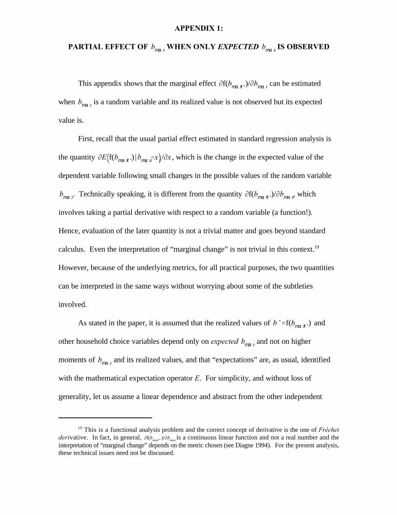
This is a functional analysis problem and the correct concept of derivative is the one of Fréchet19

derivative. In fact, in general, is a continuous linear function and not a real number and theinterpretation of “marginal change” depends on the metric chosen (see Diagne 1994). For the present analysis,these technical issues need not be discussed.

APPENDIX 1:

PARTIAL EFFECT OF WHEN ONLY EXPECTED IS OBSERVED

This appendix shows that the marginal effect can be estimated

when is a random variable and its realized value is not observed but its expected

value is.

First, recall that the usual partial effect estimated in standard regression analysis is

the quantity , which is the change in the expected value of the

dependent variable following small changes in the possible values of the random variable

. Technically speaking, it is different from the quantity , which

involves taking a partial derivative with respect to a random variable (a function!).

Hence, evaluation of the later quantity is not a trivial matter and goes beyond standard

calculus. Even the interpretation of “marginal change” is not trivial in this context. 19

However, because of the underlying metrics, for all practical purposes, the two quantities

can be interpreted in the same ways without worrying about some of the subtleties

involved.

As stated in the paper, it is assumed that the realized values of and

other household choice variables depend only on expected and not on higher

moments of and its realized values, and that “expectations” are, as usual, identified

with the mathematical expectation operator E. For simplicity, and without loss of

generality, let us assume a linear dependence and abstract from the other independent

f(bmax, .) ' $Ebmax

Mf(bmax, .)/Mbmax' $E

Mf(bmax, .)/Mbmax(h) ' $Eh bmax dbmax

Mf(bmax, .)/Mbmax(dbmax) ' $Edbmax Mf(bmax, .)/Mbmax

b ( bmax

37

variables. That is, . Thus, $ is the usual partial effect and the

coefficient to be estimated in a standard regression. Because the expectation operator is a

linear function, one has and for all random variables h,

. In particular, for a “marginal change” in of size ,

we have . In fact, can be identified with

$ and interpreted as the expected change in following an expected change in .

This proves the claim made in the paper.

p(y|x) 'jJ

j'1

H(j)Q(j)

p(j|x)p(y|x,j)

jJ

j'1

H(j)Q(j)

p(j|x)

38

The derivation of equations (8) and (9) follows from the sampling procedure and Bayes’s rule.20

(7)

APPENDIX 2:

CORRECTING FOR THE EFFECTS OF CHOICE-BASED SAMPLING

To consistently estimate the parameters of any of the equations in the system

(1)-(4), one needs to derive the probability density and conditional means under choice-

based sampling of the distribution of y|x. Although the case treated in the literature on

estimation under choice-based sampling is when the dependent variable y is used as a

stratifying variable (Manski and McFadden 1981; Amemiya 1985; Hausman and Wise

1981; Cosslett 1981, 1993), the same methods can be used to derive consistent estimators

of the population parameters when the endogenous stratifying variable is other than y (the

membership status variable in this case). If j = 1,...,J indexes the J alternative choices

defining the strata, then under choice-based sampling, the conditional probability density

and mean of y|x are given respectively by20

and

E(y|x) / myp(y|x)dy '

jJ

j'1

H(j)Q(j)

p(j|x)E(y|x,j)

jJ

j'1

H(j)Q(j)

p(j|x)

.

wj/

H(j)Q(j)

p(j|x)

jJ

j'1

H(j)Q(j)

p(j|x)

j'1,...,J ,

E(y|x) 'jJ

j'1wjE(y|x,j) .

E(y|x,j)

p(j|x)

39

(8)

(9)

(10)

If we define the choice-based-corrected conditional probability choices as

then the conditional mean of y|x under choice-based sampling can be written as a

weighted sum of the population conditional means, , where the weights are

precisely the choice-based-corrected conditional probability choices. That is,

Since in this study the population ratios, Q(j), j=1,...,J, are known (they are

obtained from the village census done prior to the survey), one can use equation (7) to

jointly and consistently estimate by maximum likelihood methods the population

parameters of the distribution of y|x,j and the conditional probability choices (after

specifying a multinomial probit or logit model for ). Except for the additional terms

involving the conditional density of y|x,j, the likelihood function resulting from equation

p(j|x)

E(y|x,j) ' "x % $jz(j) j'1,...,J .

E(y|x) '"x % jJ

j'1wj$jz(j) .

E(y|x,j)

40

The Manski-McFadden estimator estimates the population parameters of the conditional probability21

choices .

For simplicity, equation (13) does not take into account the additional terms arising from the22

simultaneity of some of the regressors in x and z(j).

(11)

(12)

(7) is the same as the one for the Manski-McFadden (1981) choice-based sampling

estimator (see, also, Amemiya 1985, 330). However, as described in this paper, a two-21

stage estimation method similar to Heckman’s two-step procedure for Tobit models is

used.

The explicit form of equation (10) for equations (1)-(4) are derived by writing the

population conditional means as

Here z(j) is a vector of alternative-specific regressors and " and $ are the parameters toj

be estimated. Hence, equation (10) becomes22

Because the alternative-specific regressors in the system of equations (1)-(4) are

comprised only of the credit program dummy variables, equation (12) can be further

simplified. Indeed, let (D ,...,D ) be the J dimensional vector of program dummies1 J

corresponding to the mutually exclusive J alternative choices defining the strata. Also, let

$jzi(j) 'jJ&1

k'1$kDk(ji) with Dk(ji)'1 if ji'k and 0 otherwise.

E(yi|xi) '"xi% jJ&1

j'1wjij

J&1

k'1$kDk(ji) '"xi%j

J&1

j'1wji

$jDji(ji) '"xi%j

J&1

j'1$jwji

i'1,...,n.

41

Again, as noted in footnote 8, equation 14 does not take into account the additional terms arising from23

the possible simultaneity of some of the regressors in x and z(j).

(13)

(14)

j designate the strata or alternative choice of the i household. Then, for the iith th

household, we have, after dropping one of the (redundant) dummy variables,

Hence, the sample analogue of equation (12) can be written as

As claimed in the paper, equation (14) shows that the choice-based sampling

correction concerns only the equations where the program dummies appear as regressors

and the correction consists simply of replacing the program dummies by the

corresponding consistently estimated choice-based-corrected conditional probability

choices. Of course, the estimated $ parameters have to be interpreted accordingly.23j

ESTIMATION OF THE CONDITIONAL PROBABILITY CHOICES

The four-alternative nested multinomial logit is specified to have two levels. In the

first level, the choice is between participation and nonparticipation in a credit program

(corresponding to choice j = 0). In the second level, which is reached only if participation

P0i/prob{ji'0} 'eX )

0i$0

e X )

0i$0 % aTi(()D,

P1i/prob{ji'1} 'eX )

1i(1

Ti((),

42

The reason for drop out may be either voluntary or exclusion because of default. However, almost24

all the past members in the sample are from SACA, a failed government agricultural credit program, theoperations of which have been taken over by MRFC. MRFC has offered defaulters from SACA the optionto join MRFC after agreeing on a rescheduling of their past SACA loans.

(15)

(16)

is the chosen alternative, the choice is between (1) joining and remaining a member of

MRFC (j = 1), (2) joining and remaining a member of the second program (j = 2), and

(3) joining either MRFC or the second program and then dropping out of the program

(i.e., being a past member; j = 3). MRFC is the only program operating in one of the24

five districts represented in the survey. Therefore, the estimation imposes the restriction

that households in that district do not have a second program choice. Allowing for

different parameter vectors for the regressors in the four alternative choices, normalizing

the coefficient for the fourth alternative to zero, and taking into account the fact that there

is no second program in one of the five districts, the four probability choices for a

household i are given by (see Amemiya 1985; Maddala 1983; Judge et al. 1985; Schmidt

and Strauss 1975)

P2i/prob{ji'2} ' (1&di)eX )

2i(2

Ti((),

P3i/prob{ji'3} '1

Ti((),

Ti(() / 1%eX )

1i(1% (1&di)eX )

2i(2 ( / ((1,(2)/ ($1/D ,$2/D)

43

(17)

(18)

and

where and . The X are vectorsji

of alternative specific regressors, d is a district dummy variable, and $ , a, and D are thei j

parameters to be estimated. McFadden’s (1981) sequential maximum likelihood

estimation for nested multinomial logit models consists of first estimating ( from

equations (16)-(18), which constitute a simple multinomial logit model (with the Manski-

Lerman weighted MLE). The estimated ( parameter is then plugged into equation (15) to

get estimates of $ , a, and D by the Manski-Lerman weighted MLE. The estimates of $ ,0 1

and $ are then obtained from the estimates ( and D. The estimation was implemented in2

GAUSS, using the Berndt et al. (1974) algorithm.

44

APPENDIX 3:

DATA AND EMPIRICAL RESULTS

214257 214257N =

FEMALEMALE

1000

900

800

700

600

500

400

300

200

100

0

-100

Formal

Informal 471471N =

InformalFormal

1000

900

800

700

600

500

400

300

200

100

0

-100

5930 5930N =

FEMALEMALE

2000

1800

1600

1400

1200

1000

800

600

400

200

0

-200

Formal

Informal 5930 5930N =

FEMALEMALE

Cre

dit l

imit

(MK

)

2000

1800

1600

1400

1200

1000

800

600

400

200

0

-200

Formal

Informal

Table 1—Formal and informal credit limits in Malawi (October 1993 to December1995)

Credit limits (Mk). All respondents Formal-sector borrowers only($1=15Mk)

Formal Informal Formal Informal

Mean 167 99 675 90Median 0 40 500 20Standard deviation 497 354 911 499Minimum 0 0 13 0Maximum 10,000 12,000 10,000 12,000

Source: IFPRI/Bunda, Rural Finance survey, 1995.

Figure 1—Distribution of formal and informal credit limits in Malawi (October1993 to December 1995): Box plot diagrams

All respondents

Formal-sector borrowers only

Notes: Box plot diagrams are interpreted as follow: For each box, 50 percent of cases have values within the box andthe solid horizontal line inside is the median. The length of the box is the interquartile range and the lowerboundary (resp upper boundary) of the box is the 25th (resp 75th) percentile. Finally, the circles are outliersand the stars are extreme values. The exchange rate is $1 = 15 Mk. Malawi’s 1995 per capita GNP is $170(i.e., 2,550 Mk, World Tables, 1997).

10859 16230N =

InformalFormal

2000

1800

1600

1400

1200

1000

800

600

400

200

0

-200

Male

Female27090N =

InformalFormal

2000

1800

1600

1400

1200

1000

800

600

400

200

0

-200

46

Table 2—Formal and informal loan sizes in Malawi (October 1993 to December1995)

Loan size (Mk). Formal Informal($1=15Mk)

Male Female All Male Female All

Mean 651 469 530 80 77 76Median 453 355 393 40 20 30Standard deviation 919 458 652 237 313 269Minimum 84 13 13 1 1 1Maximum 9,025 4,000 9,025 7,500 8,000 8,000

Source: IFPRI/Bunda, Rural Finance survey, 1995.

Figure 2—Distribution of formal and informal loan sizes in Malawi (October 1993to December 1995): Box plot diagrams

Notes: Box plot diagrams are interpreted as follow: For each box, 50 percent of cases have values within the box andthe solid horizontal line inside is the median. The length of the box is the interquartile range and the lowerboundary (resp upper boundary) of the box is the 25th (resp 75th) percentile. Finally, the circles are outliersand the stars are extreme values. The exchange rate is $1=15 Mk. Malawi’s 1995 per capita GNP is $170(i.e., 2,550 Mk, World Tables 1997).

471471N =

InformalFormal

1000

900

800

700

600

500

400

300

200

100

0

-100214257 214257N =

FEMALEMALE

1000

900

800

700

600

500

400

300

200

100

0

-100

Formal

Informal

9090N =

InformalFormal

2000

1800

1600

1400

1200

1000

800

600

400

200

0

-2005930 5930N =

FEMALEMALE

2000

1800

1600

1400

1200

1000

800

600

400

200

0

-200

Formal

Informal

47

Table 3—Formal and informal unused credit lines in Malawi (October 1993-December 1995)

Unused credit lines All respondents Formal-sector borrowers only(Mk).($1=15Mk) Formal Informal Formal Informal

Mean 49 51 148 69Median 0 10 0 10Standard deviation 245 138 474 202Minimum 0 0 0 0Maximum 6,576 4,000 6,576 4,000

Source: IFPRI/Bunda, Rural Finance survey, 1995.

Figure 3—Distribution of unused formal and informal credit lines in Malawi(October 1993 to December 1995): Box plot diagrams

All respondents

Formal-sector borrowers only

Notes: Box plot diagrams are interpreted as follow: for each box, 50 percent of cases have values within the boxand the solid horizontal line inside is the median. The length of the box is the interquartile range and thelower boundary (resp upper boundary) of the box is the 25th (resp 75th) percentile. Finally, the circles areoutliers and the stars are extreme values. The exchange rate is $1=15 Mk. Malawi’s 1995 per capita GNP is$170 (i.e., 2,550 Mk, World Tables 1997).

48

Table 4—Definition and summary statistics of variables used in the modelStandard

Variable Mean Deviation Minimum Maximum N Label

AGEH 45.82 13.76 20.0 86.0 1,885 Age of headAGLPAREA 81.35 19.02 0 100 1,885 Percent share of household ag. land out of total landCDTH3Y .26 .45 0 2 1,885 Number of deaths in household within last 3 yearsCDWAGE .11 .31 0 1 1,885 1=Has a daily wage contractCFCWAGE .09 .29 0 1 1,885 1=Has a fixed work contractCILLAC3Y .18 .52 0 5 1,885 Number of illness/accident in household in last 3 yearsCINC94 192.89 440.67 –324 4,864 1,885 Mk Total household 94 net crop incomeCPVENT3Y .51 .89 .00 8.00 1,885 Number of positive events in household in last 3 yearsCROPRISK 7.78 1.53 5 10 1,885 Index of crop risk 1 to 9CVG9495P 1.24 .34 .85 2.03 1,885 94/95 gaps within-peak season coefficient of var.CVGAPYYP .30 .06 .20 .45 1,885 Coefficient variable across years days of gaps (no rain)CWMWAGE .12 .33 0 1 1,885 1=Has a weekly/monthly wage contractDEPRATIO .49 .22 .00 1.00 1,885 Dependency ratio (population <15 & >64)DISTFA 2.33 3.75 .00 15.00 1,885 Distance to FA/CDA homeDISTPO 6.64 7.70 .00 26.00 1,885 Distance to post officeDISTPSCH 1.65 1.76 .00 5.00 1,885 Distance to primary schoolDISTTCEN 5.04 5.16 .00 15.00 1,885 Distance to trading centerDP9495 .60 .49 .00 1.00 1,885 1=1994/1995 dataDPASTMH .24 .43 0 1 1,885 1=Household is a past member of a credit programFAINRATT .34 .20 .00 2.96 1,885 Transaction cost-adjusted formal int. rateFAMTSTD 13.02 52.90 –145 846 1,885 Mk outstanding on previous period formal loanFARMLEND .05 .22 0 1 1885 1=Lender is a simple farmerFGIFTRV 4.21 22.10 0 417 1,508 Mk value of NGO gifts received by householdFLOANMAX 70.50 172.91 0 2,600 1,603 Maximum formal credit limitFLOANVAL 30.75 110.09 0 2,256 1,885 Mk value of formal loans receivedFNOCLCND .06 .23 .00 1.00 1,885 1=No condition on the formal loanFPDEFLT .09 .29 0 1 1,885 1=Has defaulted on past formal loansFWEEKDLY 1.37 2.32 .00 26.00 1,885 Formal loan weeks of delay before receiptIAMTSTD .45 5.47 –4 100 1,885 Mk outstanding on previous per. informal loanIDUEDATE .26 .44 0 1 1,885 1=Informal loan with fixed due dateILLACCDN .19 .49 0 4 1,885 Number of illness/accident in householdILOANMAX 25.14 49.39 0 743 1,511 Maximum informal credit limitILOANVAL 2.23 11.51 0 200 1,885 Mk value of informal loans receivedINOCLCND .07 .25 0 1 1,885 1=No condition on the informal loanIWEEKDLY .06 .28 .00 4.70 1,885 Informal loan weeks of delay before receiptLANDAREH 1.96 1.41 .1 13 1,885 Total hectares of household landLCGIFTG 4.01 24.52 0 720 1,508 One period lag of cumulative gifts givenLCLOANG 8.48 35.81 0 566 1,508 One period lag of cumulative loans givenLDAOWNS .43 .47 .00 1.00 1,885 Share of acres of household land owned by spouseLDPASSTH .51 .25 .0 1.0 1,885 Share of value of household assets held as landLVPASSTH .13 .20 .0 1.0 1,885 Share of value of household assets in livestockMALEHEAD .72 .45 0 1 1,885 1=Male-headed householdMALELEND .09 .29 0 1 1,885 1=Lender is a maleMRFCH .22 .42 0 1 1,885 1=Household is a current member of MRFCMUDZIH .07 .25 0 1 1,885 1=Household is a current member of MUDZI FUNDMUSCOH .07 .26 0 1 1,885 1=Household is a current member of MUSCONCLWATER .38 .48 0 1 1,885 1=No access to clean waterNGOLEND .01 .11 0 1 1,885 1=Lender is a credit club memberNWLSBUY .98 1.22 .00 4.00 1,885 Number of wholesale buyers coming to villagePCFERT95 2.13 .84 .94 6.67 1,885 1995 Chemical fertilizer price (Mk/kg)PDASOWNS .40 .46 .00 1.00 1,885 Share of value of household productive assetPEVENTN .41 .82 .00 8.00 1,885 Number of positive events in household

(continued)

49

Table 4 (continued)

StandardVariable Mean Deviation Minimum Maximum N Label

PHVKM 30.03 94.01 0 700 1,885 Distance from village of parents of headPMERW1H .16 .36 0 1 1,885 1=Household is a current member of PMERW1PMERW2H .09 .29 0 1 1,885 1=Household is a current member of PMERW2POPADL15 2.56 1.26 0 8 1,885 Adult household members between 15 and 64PPTOB95 12.17 3.98 2.00 30.00 1,885 1995 Tobacco producer price (Mk/kg)PSHMZ95 3.88 1.36 .70 7.00 1,885 1995 Hybrid maize seed price (Mk/kg)PSLMZ95 16.97 105.63 .33 2,000.00 1,885 1995 local maize seed price (Mk/kg)PSTOB95 1.40 .41 .12 4.50 1,885 1,995 Tobacco seed price (Mk/g)PSVKM 26.55 77.20 0 600 1885 Distance from village of parents of spousePVBEANS 8.12 2.86 3.70 25.00 1885 Village consumer (weighted) price of beanPVCASVA 2.78 1.51 .55 6.45 1885 Village consumer (weighted) price of cassavaPVCATL 776.77 474.93 95 3,000 1885 Village-level (weighted) prices of cattlePVCHKD 223.77 728.19 5 5,106 1885 Village-level (weighted) prices of chickenPVDRINK 12.45 10.24 2.08 53.60 1885 Village consumer (weighted) price of drinkPVGSHP 87.50 37.13 26 255 1885 Village-level (weighted) prices of goatsPVMAIZE 1.52 .95 .08 6.16 1885 Village consumer (weighted) price of maizePVMEAFSH 8.37 3.07 .73 16.01 1885 Village consumer (weighted) price meat/fishPVOTHER 6.09 4.25 .24 19.79 1885 Village consumer (weighted) price of otherPVOXEN 1,787.71 485.29 450 3,000 1885 Village-level (weighted) prices of oxenPVVEGFRT 2.21 .94 .11 6.89 1885 Village cons. (weighted) price of vegetablesRELALEND .06 .23 0 1 1885 1=Lender is a relative of borrowerRICHLEND .08 .27 0 1 1885 1=Lender is richer than borrowerSHTRADEL .04 .21 0 1 1885 1=Lender is a shopkeeper or traderSOUTH .24 .43 0 1 1885 1=Southern regionTASSETVH 2,111.13 4,187.78 130 79,991 1885 Mk total value of all assets owned by householdVPOORER .20 .40 .00 1.00 1885 1=Village is poorer than neighboring villageWSL12MHH 1.01 1.92 .00 17.33 1885 Average Weeks of sick. in last 12 months in householdYYEDUCH 4.20 3.32 .00 12.00 1885 Years of schooling of headYYEDUCS 3.14 3.05 .00 10.00 1885 Years of schooling of spouse

50

IndependentVariable

Estimated coefficients IndependentVariable

Estimated coefficients

Beta0 Beta1 Beta2 Beta0 Beta1 Beta2

CONSTANTs.e MRFCH s.e FPDEFLT s.e MUDZIH s.e MUSCOH s.e PMERW1H s.e PMERW2H s.e DMEMREJHs.e DKNOWCLBs.e PVMAIZE s.e PPTOB95 s.e PVOXEN s.e PVCATL s.e PVGSHP s.e PVCHKD s.e CDWAGE s.e CWMWAGE s.e CFCWAGE s.e LANDAREHs.e AGLPAREAs.e

-1.9049 0.1123 1.1781 0.0405-0.0681 0.0340 . . . . . . . . 0.0200 0.0375 0.0857 0.0227 0.0153 0.0074-0.0054 0.0055 0.0007 0.0000 0.0001 0.0000-0.0012 0.0005 0.0000 0.0000 0.0290 0.0242-0.0269 0.0233 0.0264 0.0203 0.0107 0.0078 0.0006 0.0006

0.7687 0.1716 . .-0.0139 0.0216 1.2087 0.0739 0.6845 0.0622 1.2931 0.0180 1.2811 0.0323 0.0303 0.0253-0.0508 0.0172 0.0035 0.0099-0.0005 0.0035-0.0005 0.0000-0.0001 0.0000-0.0009 0.0003-0.0000 0.0000 0.0502 0.0136-0.0367 0.0154 0.0338 0.0145-0.0090 0.0060 0.0004 0.0004

1.1957 0.1958 . . . . . . . . . . . . 0.3542 0.0708-0.5365 0.0404 0.0162 0.0154 0.0005 0.0056-0.0001 0.0001-0.0002 0.0001 0.0004 0.0009 0.0000 0.0000-0.0057 0.0543 0.0341 0.0449-0.0109 0.0468-0.0063 0.0141-0.0021 0.0010

TASSETVHs.e LDPASSTHs.e LVPASSTHs.e PDASOWNSs.e LDAOWNS s.e AGEH s.e MALEHEADs.e YYEDUCH s.e YYEDUCS s.e PHVKM s.e CDTH3Y s.e CILLAC3Ys.e POPADL15s.e DEPRATIOs.e NCLWATERs.e NWLSBUY s.e DISTFA s.e DISTPO s.e CROPRISKs.e

-0.0000 0.0000-0.0364 0.0466 0.0769 0.0698 0.1179 0.0769-0.0243 0.0624-0.0011 0.0008 0.1221 0.0340 0.0067 0.0049-0.0123 0.0051 0.0002 0.0001 0.0148 0.0174-0.0017 0.0280-0.0496 0.0166-0.0717 0.0461 0.0253 0.0204 0.1011 0.0128 0.0201 0.0025 0.0039 0.0017 0.0302 0.0103

-0.0000 0.0000 0.1054 0.0313 0.0590 0.0332 0.0417 0.0519-0.0136 0.0387 0.0008 0.0004 0.0019 0.0153-0.0023 0.0032 0.0006 0.0033 0.0003 0.0001 0.0053 0.0101-0.0007 0.0091 0.0148 0.0083 0.0264 0.0258 0.0528 0.0090-0.0879 0.0094-0.0077 0.0036-0.0017 0.0022 0.0299 0.0147

-0.0000 0.0000-0.0983 0.0921 0.0856 0.1567 0.0392 0.1247 0.0205 0.1092 0.0004 0.0015-0.0307 0.0566 0.0047 0.0073-0.0129 0.0081-0.0004 0.0002 0.0344 0.0354-0.0232 0.0292-0.0720 0.0209-0.2886 0.1016 0.0531 0.0421-0.0403 0.0182 0.0111 0.0039-0.0061 0.0023 0.0378 0.0164

D = 0.997 s.e: 0.503 McFadden's pseudo R-squared 0.79

Notes: The parameter a was normalized to 1 because of difficulties identifying it. The 0.997 estimate for D is practically andstatistically significantly not different from 1. Therefore, the reported results are basically for a multinomial logit model withdifferent parameter vectors (which corresponds to D = 1).

Table 5—Probability choice model parameters

51

Conditional probability of:

Not participating Participating

0.38 (0.025) 0.62 (0.025)

Conditional on participating,probability of being:

a member ofMRFC

a member ofMudzi, MUSCCO or PMERW

a past member

0.36 (0.017) 0.28 (0.02) 0.36 (0.019)

Table 6—Predicted conditional probability choices (standard errors in parentheses)

52

Independent variable

Partial changes of probability choices

MRFC Second program Past member Never been member

MRFCH s.e FPDEFLT s.e MUDZIH s.e MUSCOH s.e PMERW1H s.e PMERW2H s.e DMEMREJHs.e DKNOWCLBs.e PVMAIZE s.e PPTOB95 s.e LANDAREHs.e AGLPAREAs.e TASSETVHs.e LDPASSTHs.e LVPASSTHs.e AGEH s.e MALEHEADs.e YYEDUCH s.e YYEDUCS s.e PHVKM s.e CDTH3Y s.e CILLAC3Ys.e POPADL15s.e.DEPRATIOs.e

0.2579 0.0127-0.0121 0.0079-0.0976 0.0085-0.0661 0.0069-0.1022 0.0066-0.1016 0.0067 0.0019 0.0079 0.0197 0.0053 0.0027 0.0020-0.0010 0.0012 0.0026 0.0018 0.0001 0.0001-0.0000 0.0000-0.0137 0.0113 0.0109 0.0154-0.0003 0.0002 0.0231 0.0075 0.0014 0.0010-0.0024 0.0011 0.0000 0.0000 0.0025 0.0040-0.0003 0.0065-0.0104 0.0038-0.0154 0.0106

-0.1114 0.0057 0.0022 0.0043 0.1940 0.0176 0.1158 0.0142 0.2055 0.0139 0.2039 0.0139 0.0033 0.0039-0.0131 0.0031-0.0004 0.0017 0.0003 0.0006-0.0021 0.0010 0.0000 0.0001 0.0000 0.0000 0.0182 0.0066 0.0040 0.0065 0.0002 0.0001-0.0074 0.0032-0.0008 0.0004 0.0009 0.0005 0.0000 0.0000-0.0002 0.0020-0.0000 0.0028 0.0054 0.0017 0.0086 0.0053

-0.1465 0.0081 0.0099 0.0053-0.0964 0.0094-0.0496 0.0076-0.1033 0.0076-0.1023 0.0076-0.0052 0.0065-0.0066 0.0037-0.0023 0.0011 0.0007 0.0009-0.0006 0.0013-0.0001 0.0001 0.0000 0.0000-0.0045 0.0069-0.0149 0.0112 0.0001 0.0001-0.0157 0.0054-0.0006 0.0009 0.0015 0.0009-0.0000 0.0000-0.0023 0.0027 0.0003 0.0040 0.0050 0.0026 0.0068 0.0072

-0.1120 0.0063 0.0063 0.0032-0.0803 0.0082-0.0384 0.0063-0.0872 0.0066-0.0862 0.0065 0.0775 0.0193-0.1225 0.0125 0.0061 0.0059 0.0002 0.0022-0.0024 0.0054-0.0008 0.0004-0.0000 0.0000-0.0371 0.0351 0.0314 0.0594 0.0002 0.0006-0.0168 0.0136 0.0018 0.0028-0.0050 0.0031-0.0001 0.0001 0.0131 0.0137-0.0089 0.0112-0.0279 0.0080-0.1124 0.0409

Table 7—Matrix of partial changes of probability choices with respect to changes inselected independent variables

53

Independentvariable

Directeffect a

Indirect effectthrough theprobabilitychoices

Totaleffect

Independentvariable

Directeffect a

Indirect effectthrough theprobabilitychoices

Totaleffect

CONSTANTs.e MRFCH s.e MUDZIH s.e MUSCOH s.e PMERW1H s.e PMERW2H s.e WMRFC s.e WPROG2 s.e WDPAST s.e FPDEFLT s.e DP9495 s.e LANDAREHs.e AGLPAREAs.e TASSETVHs.e LDPASSTHs.e LVPASSTHs.e YYEDUCH s.e YYEDUCS s.e

-2534.62343.0319 . . . . . . . . . . 2913.05 309.66 2928.46 322.59 2790.41 328.91-20.7784 13.8852-10.8881 4.6691 7.0622 5.7895 0.2929 0.3149 0.0017 0.0033-79.3011 28.5800-46.0946 34.1626 -0.0618 2.4691 2.4703 2.7511

. . 19.6259 3.9254 54.0689 7.6468 33.7595 6.2161 56.8125 8.0875 56.4310 7.7808 . . . . . . -2.7817 0.8726 . . 0.4440 0.8846 0.2658 0.0757 0.0009 0.0004 15.3997 6.2558 -7.2518 10.3868 -0.6180 0.5209 1.5237 0.5690

-2534.62343.0319 19.6259 3.9254 54.0689 7.6468 33.7595 6.2161 56.8125 8.0875 56.4310 7.7808 2913.05 309.66 2928.46 322.59 2790.41 328.91-23.5600 13.7048-10.8881 4.6691 7.5062 6.0081 0.5587 0.3190 0.0026 0.0032-63.9014 29.9756-53.3463 37.0432 -0.6798 2.4549 3.9940 2.7320

POPADL15 s.e DEPRATIO s.e AGEH s.e MALEHEAD s.e PVMAIZE s.e PPTOB95 s.e PVOXEN s.e PVCATL s.e PVGSHP s.e PVCHKD s.e NWLSBUY s.e DISTFA s.e DISTPO s.e DISTPSCH s.e DISTTCEN s.e SOUTH s.e

-19.6817 5.4872-90.6065 33.2885 -0.0063 0.5270-18.3682 16.3404 5.9506 4.5373 3.9528 2.9707 0.0062 0.0102 0.0341 0.0143 -0.8954 0.3711 0.0218 0.0188 21.7647 7.6705 -4.1433 2.0048 6.7724 2.2097 6.1053 5.9583 -5.5751 2.2008-72.9070 47.1576

9.0646 1.575635.7310 7.5305-0.0244 0.0977 5.8149 2.4588-1.7266 0.9757-0.0950 0.4106-0.0042 0.0045 0.0183 0.0037-0.0881 0.0635-0.0022 0.0026 1.7904 1.2270-1.5329 0.2872 0.6807 0.1656 . . . . . .

-10.6171 5.7452-54.8756 34.9863 -0.0307 0.5538-12.5533 16.5945 4.2240 4.8009 3.8578 2.9262 0.0020 0.0111 0.0524 0.0146 -0.9835 0.3691 0.0196 0.0189 23.5552 7.8415 -5.6762 2.0243 7.4531 2.2246 6.1053 5.9583 -5.5751 2.2008-72.9070 47.1576

R-squared: 0.20F-stat. (all coefficients): F = 7.38(49,1458)

F-stat for the program dummies: F = 50.41(3,1505)

F-stat for all instruments : F = 9.15 b(27,1481)

The column of direct effects corresponds to the estimated coefficients of the variables included in the equations.a

These are the exogenous regressors used as instruments in some of the other equations of the system: WMRFC WPROG2 WPASTb

PVMAIZE PVCASVA PVBEANS PVVEGFRT PVMEAFSH PVDRINK PVOTHER PPTOB95 PVOXEN PVCATL PVGSHPPVCHKD CDTH3Y CILLAC3Y PHVKM PSVKM NCLWATER NWLSBUY DISTFA DISTPO DISTPSCH DISTTCENCROPRISK CVGAPYYP

Table 8—Formal credit limit equation (FLOANMAX): Matrix of direct and indirectpartial effects of selected variables

54

Independent variable Partial effect Independent variable Partial effect

CONSTANTs.e RELALENDs.e SHTRADELs.e FARMLENDs.e MALELENDs.e RICHLENDs.e SVLGLENDs.e NGOLEND s.e FPDEFLT s.e DP9495 s.eLANDAREHs.e AGLPAREAs.e TASSETVHs.e

88.7567 39.7190 0.7911 5.3971 -9.8742 9.5635 -7.9653 5.9776 10.0884 6.4531 8.4306 10.0360 8.2313 5.6507 24.5043 9.7688 2.1497 3.5205 -4.0459 2.3682 5.9994 2.0169 -0.0779 0.0937 -0.0000 0.0005

LDPASSTHs.e LVPASSTHs.e YYEDUCH s.e YYEDUCS s.e POPADL15s.e DEPRATIOs.e AGEH s.e MALEHEADs.e DISTPO s.e PVMAIZE s.e PPTOB95 s.e PVOXEN s.e PVCATL s.e PVGSHP s.e PVCHKD s.e

-26.9211 8.4329-26.2156 8.4539 0.8625 0.7060 0.1897 0.6052 -0.9945 1.3143-17.6419 6.5542 -0.2330 0.1454 -4.3006 3.9398 -0.6407 0.4969 -1.0145 2.3822 -0.8183 0.4166 0.0052 0.0038 0.0039 0.0052 -0.0618 0.0541 0.0062 0.0051

R-squared : 0.12F-stat. (all coefficients): F = 3.47 (56,1451)

F-stat lender characteristics : F = 3.88a(7,1501)

F-stat for all instruments : F = 2.60 b(31,1477)

RELALEND SHTRADEL FARMLEND MALELEND RICHLEND SVLGLEND NGOLENDa

These are the exogenous regressors used as instruments in some of the other equations of the system:b

RELALEND SHTRADEL FARMLEND MALELEND RICHLEND SVLGLEND NGOLEND PVMAIZEPVCASVA PVBEANS PVVEGFRT PVMEAFSH PVDRINK PVOTHER PPTOB95 PVOXENPVCATL PVGSHP PVCHKD CDTH3Y CILLAC3Y PHVKM PSVKM NCLWATER NWLSBUYDISTFA DISTPO DISTPSCH DISTTCEN CROPRISK CVGAPYYP.

Table 9—Informal credit limit equation (ILOANMAX): Estimated coefficients ofselected variables (partial effects)

55

Independentvariable

Directeffect a

Indirect effect through Totaleffect

Independentvariable

Directeffect a

Indirect effect through Totaleffect

FLOANMAX ILOANMAX FLOANMAX ILOANMAX

CONSTANTs.e FLOANMAXs.e ILOANMAXs.e MRFCH s.e MUDZIH s.e MUSCOH s.e PMERW1H s.e PMERW2H s.e WMRFC s.e WPROG2 s.e WDPAST s.e DP9495 s.e FWEEKDLYs.e FNOCLCNDs.e IWEEKDLYs.e IDUEDATEs.e INOCLCNDs.e IAMTSTD s.e FAMTSTD s.e FPDEFLT s.e FAINRATTs.e

2.1633 17.2245 0.4887 0.0873 -0.0411 0.0435 . . . . . . . . . . . . . . . . 13.6721 2.8850 -0.7499 1.0541 16.4898 13.2291 4.4648 4.0671 63.6118 9.6131-27.7287 6.5529 0.0597 0.1718 -0.1085 0.0571 . . 2.1165 15.5655

. . . . . . 9.5921 2.0898 26.4259 3.8919 16.4998 3.0489 27.7668 4.0558 27.5804 3.8885 1423.73 192.06 1431.26 191.69 1363.80 196.57 -5.3215 2.1320 . . . . . . . . . . . . . .-11.5148 7.5773 . .

. . . . . . . . . . . . . . . . . . . . . . 0.1662 0.2369 . . . . . . . . . . . . . .-0.0883 0.2636 . .

2.1633 17.2245 0.4887 0.0873 -0.0411 0.0435 9.5921 2.0898 26.4259 3.8919 16.4998 3.0489 27.7668 4.0558 27.5804 3.8885 1423.73 192.06 1431.26 191.69 1363.80 196.57 8.5168 3.8359 -0.7499 1.0541 16.4898 13.2291 4.4648 4.0671 63.6118 9.6131-27.7287 6.5529 0.0597 0.1718 -0.1085 0.0571-11.6032 7.5652 2.1165 15.5655

PVMAIZE s.e PPTOB95 s.e PSTOB95 s.e PCFERT95s.e PSLMZ95 s.e PSHMZ95 s.e LANDAREHs.e AGLPAREAs.e TASSETVHs.e LDPASSTHs.e LVPASSTHs.e YYEDUCH s.e YYEDUCS s.e POPADL15s.e DEPRATIOs.e AGEH s.e MALEHEADs.e SOUTH s.e

4.6982 2.3373-0.5920 0.6393 6.8688 3.7419 4.3571 1.7454-0.0203 0.1641-1.4519 1.1416 1.3184 2.1390-0.0822 0.0995 0.0007 0.0006-7.3556 8.539820.4063 9.5880-1.4005 0.8164-0.3242 0.6678-3.0591 2.136218.923210.6739-0.1029 0.1572 0.6103 4.8669 3.4651 7.3878

2.0645 2.6874 1.8855 1.4113 . . . . . . . . 3.6686 3.2649 0.2731 0.1586 0.0013 0.0018-31.2315 15.3376-26.0728 21.5138 -0.3323 1.2185 1.9520 1.3535 -5.1890 2.9123-26.8202 18.6753 -0.0150 0.2720 -6.1354 7.8765-35.6329 23.0927

0.0417 0.1794 0.0336 0.0463 . . . . . . . .-0.2465 0.2732 0.0032 0.0066 0.0000 0.0000 1.1061 1.3246 1.0771 1.3185-0.0354 0.0638-0.0078 0.0412 0.0409 0.1085 0.7248 0.8437 0.0096 0.0136 0.1767 0.3420 0.7590 1.1775

6.8043 2.9309 1.3271 1.6583 6.8688 3.7419 4.3571 1.7454 -0.0203 0.1641 -1.4519 1.1416 4.7405 3.7103 0.1941 0.1666 0.0020 0.0022-37.4811 16.2740-45.4020 23.0834 -1.7682 1.3786 1.6201 1.3462 -8.2073 3.4768-45.0186 20.2506 -0.1084 0.2711 -5.3483 9.1147-31.4088 21.6019

R-squared: 0.33F-stat.(all coefficients): F = 16.40(44,1463)

F-stat. for the regressors used as instruments in other equations: F =(13,1495)

1.36

Wu-Hausman Chi-squared statistics for exogeneity : x = 0.58 b(9)

Durbin Chi-squared statistics for exogeneity : x = 1.39b(9)

Basmann's Chi-squared statistics for the overidentifying restrictions :c

x = 49.98 (60)

The column of direct effects corresponds to the estimated coefficients of the variables included in the equations.a

Endogenous regressors: FLOANMAX ILOANMAX IAMTSTD FAMTSTD CINC94 FGIFTRV CDWAGE CWMWAGE CFCWAGE.b

Instruments tested: WMRFC WPROG2 WPAST RELALEND SHTRADEL FARMLEND MALELEND RICHLEND SVLGLEND NGOLENDc

PVOXEN PVCATL PVGSHP PVCHKD PHVKM PSVKM NCLWATER LATRINE NWLSBUY DISTFA DISTPO DISTPSCH DISTTCENCROPRISK CVGAPYYP.

Table 10—Formal credit demand equation (FLOANVAL): Matrix of direct andindirect partial effects of selected variables

56

IndependentVariable

Directeffect a

Indirect effect through Totaleffect

Independentvariable

Directeffect a

Indirect effect throughTotaleffectFLOANMAX ILOANMAX FLOANMAX ILOANMAX

CONSTANTs.e FLOANMAXs.e ILOANMAXs.e MRFCH s.e MUDZIH s.e MUSCOH s.e PMERW1H s.e PMERW2H s.e WMRFC s.e WPROG2 s.e WDPAST s.e DP9495 s.e FWEEKDLYs.e FNOCLCNDs.e IWEEKDLYs.e IDUEDATEs.e INOCLCNDs.e IAMTSTD s.e FAMTSTD s.e FPDEFLT s.e FAINRATTs.e

0.0570 2.9869-0.0034 0.0019 0.0680 0.0227 . . . . . . . . . . . . . . . .-0.0731 0.4805 0.0000 0.0000-0.1278 0.1597-1.2613 0.8090 6.5236 2.9264 1.5294 0.822119.4587 2.4285-0.1046 0.0838 0.0025 0.0036 1.7213 1.8740

. . . . . . -0.0677 0.0172 -0.1865 0.0431 -0.1165 0.0338 -0.1960 0.0450 -0.1947 0.0435-10.0494 3.0750-10.1025 3.0391 -9.6263 3.0359 0.0376 0.0213 0.0813 0.0671 . . . . . . . . . . . . . . . .

. . . . . . . . . . . . . . . . . . . . . .-0.2751 0.2198 0.1461 0.2931 . . . . . . . . . . . . . . . .

0.0570 2.9869 -0.0034 0.0019 0.0680 0.0227 -0.0677 0.0172 -0.1865 0.0431 -0.1165 0.0338 -0.1960 0.0450 -0.1947 0.0435-10.0494 3.0750-10.1025 3.0391 -9.6263 3.0359 -0.3106 0.4886 0.2274 0.2930 -0.1278 0.1597 -1.2613 0.8090 6.5236 2.9264 1.5294 0.8221

19.4587 2.4285 -0.1046 0.0838 0.0025 0.0036 1.7213 1.8740

PVMAIZE s.e PPTOB95 s.e PSTOB95 s.e PCFERT95s.e PSLMZ95 s.e PSHMZ95 s.e LANDAREHs.e AGLPAREAs.e TASSETVHs.e LDPASSTHs.e LVPASSTHs.e YYEDUCH s.e YYEDUCS s.e POPADL15s.e DEPRATIOs.e AGEH s.e MALEHEADs.e SOUTH s.e

0.0001 0.2500 0.0012 0.0523-0.6294 0.5177-0.0204 0.2696 0.0012 0.0067-0.0163 0.1761-0.1317 0.3408-0.0193 0.0170 0.0002 0.0002 2.3883 1.1688 1.3474 1.2919-0.0265 0.1554 0.1984 0.1130-0.3012 0.2459-0.2360 1.3061 0.0151 0.0228 0.1279 0.7859 2.0511 1.1483

-0.0146 0.0221-0.0133 0.0131 . . . . . . . .-0.0259 0.0292-0.0019 0.0014-0.0000 0.0000 0.2204 0.1758 0.1840 0.1786 0.0023 0.0087-0.0138 0.0104 0.0366 0.0239 0.1893 0.1389 0.0001 0.0019 0.0433 0.0596 0.2515 0.2050

-0.0690 0.1594-0.0556 0.0318 . . . . . . . . 0.4079 0.1765-0.0053 0.0059-0.0000 0.0000-1.8303 0.6484-1.7823 0.6994 0.0586 0.0500 0.0129 0.0490-0.0676 0.1092-1.1994 0.6180-0.0158 0.0133-0.2924 0.2976-1.2559 0.8844

-0.0834 0.2560-0.0678 0.0612-0.6294 0.5177-0.0204 0.2696 0.0012 0.0067-0.0163 0.1761 0.2503 0.3205-0.0265 0.0180 0.0002 0.0002 0.7785 1.1080-0.2509 1.2871 0.0345 0.1788 0.1975 0.1272-0.3322 0.2702-1.2461 1.3453-0.0006 0.0217-0.1212 0.8512 1.0467 1.6091

R-squared: 0.35F-stat.(all coefficients): F = 18(44,1463)

F-stat. for the regressors used as instruments in other equations: F = 1.14 (13,1495)

Wu-Hausman Chi-squared statistics for exogeneity : x = 1.02 b(9)

Durbin Chi-squared statistics for exogeneity : x = 1.12b(9)

Basmann's Chi-squared statistics for the overidentifying restrictions :c

x = 102.83 (60)

The column of direct effects corresponds to the estimated coefficients of the variables included in the equations.a

Endogenous regressors: FLOANMAX ILOANMAX IAMTSTD FAMTSTD CINC94 FGIFTRV CDWAGE CWMWAGE CFCWAGEb

Instruments tested: WMRFC WPROG2 WPAST RELALEND SHTRADEL FARMLEND MALELEND RICHLEND SVLGLEND NGOLENDc

PVOXEN PVCATL PVGSHP PVCHKD PHVKM PSVKM NCLWATER LATRINE NWLSBUY DISTFA DISTPO DISTPSCH DISTTCENCROPRISK CVGAPYYP.

Table 11—Informal credit demand equation (ILOANVAL): Matrix of direct andindirect partial effects of selected variables

57

REFERENCES

Adams, D. W., and R. C. Vogel. 1985. Rural financial markets in low-income countries:

Recent controversies and lessons. World Development 14 (4): 477–487.

Adams, D. W., D. H. Graham, and J. D. von Pischke, eds. 1984. Undermining rural

development with cheap credit. Boulder, Colo., U.S.A.: Westview Press.

Alderman, H., and C. H. Paxson. 1992. Do the poor insure? A synthesis of the

literature on risk and consumption in developing countries. Discussion Paper 164.

Princeton, N.J., U.S.A.: Princeton University, Woodrow Wilson School of Public

and International Affairs.

Amemiya, T. 1985. Advanced econometrics. Cambridge, Mass., U.S.A.: Harvard

University Press.

Avery, R. B. 1981. Estimating credit constraints by switching regression. In Structural

analysis of discrete data with econometric applications, ed. C. F. Manski and D.

McFadden. Cambridge, Mass., U.S.A.: Massachusetts Institute of Technology

Press.

Barham, B., and S. Boucher. 1994. Credit constraints, credit unions, and small-scale

producers in Guatemala. Photocopy.

Berndt, E. K., B. H. Hall, R. H. Hall, and J. A. Hausman. 1974. Estimation and

inference in nonlinear structural models. Annals of Economic and Social

Measurement 3: 653–665.

58

Besley, T. 1995. Savings, credit and insurance. In Handbook of development economics,

Vol. III, ed. J. Behrman and T. N. Srinivasan. Amsterdam and New York:

Elsevier.

Braverman, A., and J. L. Guasch. 1986. Rural credit markets and institutions in

developing countries: Lessons for policy analysis from practice and modern theory.

World Development 14 (10/11): 1253–1267.

Browning, M., and A. Lusardi. 1996. Household saving: Micro theories and micro

facts. Journal of Economic Literature 4: 1797–1855.

Coate, S., and M. Ravallion. 1993. Reciprocity without commitment: Characterization

and performance of informal insurance arrangements. Journal of Development

Economics 40 (1): 1–24.

Cosslett, S. 1981. Efficient estimation of discrete-choice models. In Structural analysis

of discrete data with econometric applications, ed. C. F. Manski and D. McFadden.

Cambridge, Mass., U.S.A.: Massachusetts Institute of Technology Press.

Cosslett, S. 1993. Estimation from endogenously stratified samples. In Handbook of

Statistics, Vol. 11, ed. G. S. Maddala, C. R. Rao, and H. D. Vinod. Amsterdam:

Elsevier Science Publishers.

Deaton, A. 1989. Savings in developing countries: Theory and review. In Proceedings

of the World Bank Annual Conference on Development Economics, ed. S. Fischer

and D. de Tray, 61-96. Washington, D.C.: World Bank.

59

Diagne, A. 1994. Consumer behavior and welfare measurement under uncertainty:

Theory and empirical evidence from Senegal. Unpublished Ph.D. diss., Michigan

State University, Department of Agricultural Economics and Department of

Economics, East Lansing, Mich., U.S.A.

Diagne, A. 1996. Measuring access to credit and its impacts on household food security:

Some methodological notes. Paper presented at 1996 annual meeting of The

American Agricultural Economic Association (AAEA), San Antonio, Texas.

Diagne, A., M. Zeller, and C. Mataya. 1996. Rural financial markets and household food

security: Impacts of access to credit on the socioeconomic situation of rural

households in Malawi. Final report submitted to the Ministry for Women, Children

Affairs, Community Development and Social Welfare, and to the German Agency

for Technical Cooperation in Malawi. Bunda College of Agriculture, University of

Malawi, and International Food Policy Research Institute, Washington, D.C.

Diagne, A., M. Zeller, and M. Sharma. 1997. Empirical measurements of households'

access to credit and credit constraints in developing countries: Methodological

issues and evidence. International Food Policy Research Institute, Washington,

D.C. Photocopy.

Fafchamps, M. 1992. Solidarity networks in pre-industrial societies: Rational peasants

with a moral economy. Economic Development and Cultural Change 41 (1):

147–174.

60

Feder G., L. J. Lau, J. Y. Lin, and X. Luo. 1990. The relationship between credit and

productivity in Chinese agriculture: A microeconomic model of disequilibrium.

American Journal of Agricultural Economics 72 (5): 1151-1157.

Freixas, X., and J. C. Rochet. 1997. Microeconomics of banking. Cambridge, Mass.:

Massachusetts Institute of Technology Press.

Gersovitz, M. 1988. Savings and development. In H. Chenery and T. N. Srinivasan,

eds., Handbook of development economics, Vol. I, ed. H. Chenery and T. N.

Srinivasan. Amsterdam: Elsevier.

Hausman, J. A., and D. A. Wise. 1981. Stratification on endogenous variables and

estimation: The Gary income maintenance experiment. In Structural analysis of

discrete date with econometric applications, ed. C. F. Manski and D. McFadden.

Cambridge, Mass., U.S.A.: Massachusetts Institute of Technology Press.

Jappelli, T. 1990. Who is credit constrained in the U.S. economy? The Quarterly

Journal of Economics CV (1) (February): 219–234.

Jeong, J., and G. S. Maddala. 1993. A perspective on application of bootstrap methods

in econometrics. In Handbook of statistics, Vol. 11, ed. G. S. Maddala, C. R. Rao,

and H. D. Vinod. Amsterdam: Elsevier Science Publishers.

Judge, G., W. E. Griffiths, R. Carter, H. Lutkepohl, and T. Lee. 1985. The theory and

practice of econometrics, 2d edition. New York: John Wiley and Sons.

61

Kochar, A. 1997. Explaining poverty: An empirical analysis of the effects of ill-health

and uncertainty on the savings of rural Pakistani households. Department of

Economics, Stanford University, Stanford, Calif., U.S.A. Photocopy.

Lund, S. M., and M. Fafchamps. 1997. Risk-sharing networks in rural Philippines.

Department of Economics, Stanford University, Stanford, Calif., U.S.A.

Photocopy.

Maddala, G. S. 1983. Limited dependent and qualitative variables in econometrics.

Cambridge: Cambridge University Press.

Manski, C. F., and D. McFadden. 1981. Alternative estimators and sample designs for

discrete choice analysis. In Structural analysis of discrete data with econometric

applications, ed. C. F. Manski and D. McFadden. Cambridge, Mass., U.S.A.:

Massachusetts Institute of Technology Press.

McFadden, D. 1981. Econometric models of probabilistic choice. In Structural analysis

of discrete data with econometric applications, ed. C. F. Manski and D. McFadden.

Cambridge, Mass., U.S.A.: Massachusetts Institute of Technology Press.

Schmidt, P., and R. Strauss. 1975. The prediction of occupation using multiple logit

models. International Economic Review 16: 471–486.

Staiger, D., and J. H. Stock. 1997. Instrumental variable regression with weak

instruments. Econometrica 65 (3): 557–586.

Stiglitz, J. E., and A. Weiss. 1981. Credit rationing in markets with imperfect

information. American Economic Review 71 (3): 393–410.

62

Townsend, R. M. 1994. Risk and insurance in Village India. Econometrica 62 (3):

539–591.

Udry, C. 1994. Risk and insurance in a rural credit market. Review of Economic Studies

61 (3): 495–526.

Udry, C. 1995. Risk and saving in northern Nigeria. American Economic Review 85 (5):

1287–1300.

Zeller, M. 1994. Determinants of credit rationing: A study of informal lenders and

formal groups in Madagascar. World Development 22 (12): 1895–1907.

Zeller, M., A. Diagne, and C. Mataya. 1997. Market access by smallholder farmers in

Malawi: Implications for technology adoption, agricultural productivity, and crop

income. Paper presented at the XXIII International Conference of Agricultural

Economists, August 10-16, Sacramento, Calif., U.S.A. (Forthcoming in a special

issue of Agricultural Economics.)

Zeller, M., G. Schrieder, J. von Braun, and F. Heidhues. 1997. Rural finance for food

security for the poor: Implications for research and policy. Food Policy Review

No. 4. Washington, D.C.: International Food Policy Research Institute.

Zeller, M., A. Ahmed, S. Babu, S. Broca, A. Diagne, and M. Sharma. 1996. Rural

financial policies for food security of the poor: Methodologies for a multicountry

research project. Food Consumption and Nutrition Division Discussion Paper 11.

International Food Policy Research Institute, Washington, D.C. Photocopy.