Determinants of Group Size in Primates: A General Model · 2020-05-14 · The principal analysis...

proceedings of the British Academy, 88, 33-51

Determinants of Group Size in Primates:

A General Model

R. I. M. DUNBAR Department of Psychology, University of Liverpool,

PO Box 147, Liverpool, L69 3BX

Keywords: group size; systems model; time budgets; baboons; chimpanzees.

Summary. Significant constraints are placed on group size by local habitat conditions as a consequence of both the selection pressures that act on the animals and the design of their physiological systems. I use a linear programming approach to develop a model of habitat-specific minimum and maximum group sizes for baboons. Three main variables define the state space of realizable group sizes. These are the maximum group size withm which the animals can still balance their time budgets (the maximum ecologically tolerable group size), the minimum group size that reduces predation risk to some (undefined) acceptable level (the minimum permissible group size) and the maximum group size that animals’ neocortex size will allow them to maintain as a coherent stable social entity (the cognitive group size). Similar models have also been developed for gelada and chimpanzees. Once group size can be determined for a particular habitat, a number of other behavioural patterns can be determined as a consequence of well-understood general principles. I illustrate this with the example of male mating strategies.

OVER THE LAST TWO DECADES, our understanding of primate behaviour, and the selection forces acting on it, has grown spectacularly, thanks largely to the shift in emphasis generated by sociobiology during the early 1970s.

0 The British Academy 1996.

Copyright © British Academy 1996 – all rights reserved

34 R. I. M. Dunbar

Being able to view behavioural interactions from a strategic (or goal- directed) perspective opened up layers of complexity in animal behaviour that the traditional stimulus-response analyses of classical ethology had been unable to tap.

What we have tended to overlook, however, is the fact that many animals live in groups. The size, composition and dispersion of groups imposes limits on the range of options open to any given individual. These demographic factors are, in turn, largely a consequence of the local ecology interacting with the species’ ecological adaptations.

It is important to understand that the optimal group size is habitat- specific: it is a consequence of the way in which the particular environmental and climatic variables characteristic of a given habitat influence the behavioural ecology of the animal in question. Hitherto, attempts to explain social evolution have too often tended to view mating systems and grouping patterns as species-specific phenomena. Variance around the species typical value has often been viewed as little more than inevitable biological error. The assumption adopted here is that variations in group size are a direct consequence of optimisation decisions by the animals. Indeed, it is precisely the variation in group size across habitats and, within habitats, through time that we are trying to explain.

Group size is, of course, a consequence of decisions made by animals about the optimal size for groups in a given habitat. The costs and benefits on which this decision is based are a function of local environmental conditions. Strictly speaking, of course, the choice of optimal group size may itself be a consequence of the costs and benefits of the behavioural options open to an animal in terms of mating and parenting. Group size may, for example, influence fertility rates (van Schaik 1983), and so alter the anticipated gains of different mating strategies. Nonetheless, there is a useful sense in which we can see decisions about group size as antecedent to the decisions that an animal makes about mate choice and parenting effort. In effect, these strictly behavioural decisions are made in the context of prior decisions about grouping patterns (Dunbar 1988).

In this paper, I summarize our attempts to build functional models of primate socio-ecological systems designed to explore these issues. Unlike the micro-economic models characteristic of much of behavioural ecology over the past 30 years, these models owe more to the macro-economic approach favoured by the systems ecologists of the 1960s. Their principal purpose is to allow us to explore the relationship between environmental parameters and demographic variables. While we understand that the relationships involved are in fact mediated by conventional optimality decisions, our interest lies not in the optimization processes themselves (though these must ultimately be part of the story) but in the consequences of these decisions. Once we can


A MODEL OF GROUP SIZE IN PRIMATES 35

understand these, we will have a much clearer idea of the systemic constraints that act on individuals’ choices at the strategic level.

The model I outline here is based on studies of baboons. We are, however, also building similar models for several other taxa. I shall allude to an earlier model developed for gelada, as well as to one currently being developed for chimpanzees by Daisy Williamson (1996). In addition, we have also started work on a similar model for gibbons (Sear 1994). In each case, I conceive the core problem as identifying the determinants of group size. Once group size is determined, a number of fairly straightforward lifehistory considerations dictate the composition and reproductive characteristics of the group.

A LINEAR PROGRAMMING MODEL OF GROUP SIZE

We can approach the problem of optimal group sizes by considering it as a linear programming model. This assumes that the optimal group size is the intersection of a set of benefit and cost equations together with a number of constraints. These create a region of possible group sizes (the range of realizable group sizes) within the state space created by the range of conceivable group sizes: the zone of realizable group sizes must lie above the line generated by the benefit equation(s), and below those generated by the cost and constraint equations.

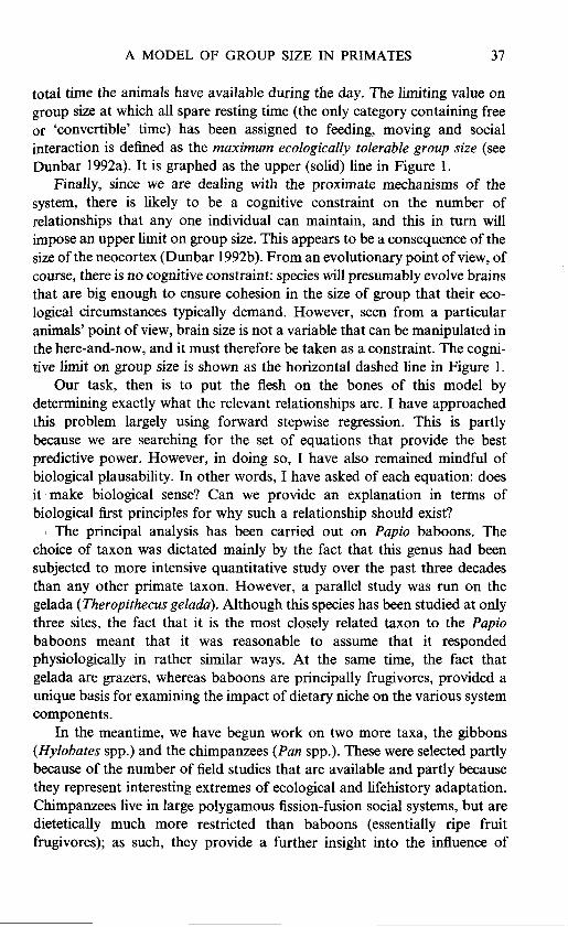
The basic model is shown in Figure 1. Here, group size is plotted against a notional environmental variable (e.g. rainfall). Strictly speaking, this should be a three-dimensional graph with fitness (or lifetime reproductive success) emerging out of the page at right angles to the other two dimensions. Each of the cost, benefit and constraint curves can then be represented more correctly as a surface in three-dimensions. Since this is difficult to show, it is simpler to illustrate the main points when the surfaces are represented by their projections in two dimensions. All points on a line are thus isometric with respect to fitness: each line represents the point at which fitness drops below some minimally acceptable level. Fitness increases above the benefit curve and it also increases below the cost and constraint curves.

The curves themselves need some interpretation. I assume that the benefit curve represents the selective advantage(s) of group size. For primates, these are usually understood to be either protection from predation risk or defence of resources (van Schaik 1983; Wrangham 1980, 1987; Dunbar 1988). Irrespective of which of these hypotheses is in fact correct, fitness increases with increasing group size. This is because both the risk of predation and the defendability of a resource increase monotonically


36 R. I. M . Dunbar

Figure

120 - Maximum Ecologically

Rainfall (mm) Linear programming model of group size. Group size is plotted against a notion;

environmental variable (in this case, meanannual rainfall). The range of realizable group sizes (harchedarea) is defmed by the minima set by the benefit variables and the maxima set by the cost and constraint variables. In this model, only one graph is shown for each type of variable. The plotted values for the maximum and minimum group sizes are those predicted by the baboon model at 25°C (approximate centre of the taxon’s preferred thermal zone). The cognitive constraint is that set by the relationship between observed mean group size and relative neocortex volume, and is almost certainly an underestimate of the true maximum cognitive group size.

with the size of the group. However, predation risk will always set a lower limit on the minimum group size than the demands of territorial defence, because the latter will inevitably tend to force the population into an arms race in which minimum group sizes are driven upwards towards the maximum tolerable by the spiralling effects of between-group competition. I define the size of group that reduces predation risk to some constant tolerable level as the minimum permissible group size. This is shown as the lower broken line in Figure 1.

However, the benefits that derive from grouping are necessarily offset by the costs of grouping. These come in two distinct kinds: direct (those due to competition and harassment, often reflected in reduced fecundity) and indirect (those that arise from the additional costs of servicing larger groups, such as increased day journey lengths and the additional feeding time required to fuel these, as well as the social time required to ensure the social cohesion of the group). Taken together, these will impose an upper limit on the size of the group that can remain together. This will arise partly from the marginal cost of reduced fecundity that females are unwilling to bear when group size exceeds some critical threshold. However, an important constraint may be imposed by the fact that the increased feeding, moving and social time requirements demanded by large groups may exceed the



total time the animals have available during the day. The limiting value on group size at which all spare resting time (the only category containing free or ‘convertible’ time) has been assigned to feeding, moving and social interaction is defined as the maximum ecologically tolerable group size (see Dunbar 1992a). It is graphed as the upper (solid) line in Figure 1.

Finally, since we are dealing with the proximate mechanisms of the system, there is likely to be a cognitive constraint on the number of relationships that any one individual can maintain, and this in turn will impose an upper limit on group size. This appears to be a consequence of the size of the neocortex (Dunbar 1992b). From an evolutionary point of view, of course, there is no cognitive constraint: species will presumably evolve brains that are big enough to ensure cohesion in the size of group that their ecological circumstances typically demand. However, seen from a particular animals’ point of view, brain size is not a variable that can be manipulated in the here-and-now, and it must therefore be taken as a constraint. The cognitive limit on group size is shown as the horizontal dashed line in Figure 1.

Our task, then is to put the flesh on the bones of this model by determining exactly what the relevant relationships are. I have approached this problem largely using forward stepwise regression. This is partly because we are searching for the set of equations that provide the best predictive power. However, in doing so, I have also remained mindful of biological plausability. In other words, I have asked of each equation: does it make biological sense? Can we provide an explanation in terms of biological first principles for why such a relationship should exist?

The principal analysis has been carried out on Papio baboons. The choice of taxon was dictated mainly by the fact that this genus had been subjected to more intensive quantitative study over the past three decades than any other primate taxon. However, a parallel study was run on the gelada (Theropithecus gelada). Although this species has been studied at only three sites, the fact that it is the most closely related taxon to the Papiu baboons meant that it was reasonable to assume that it responded physiologically in rather similar ways. At the same time, the fact that gelada are grazers, whereas baboons are principally frugivores, provided a unique basis for examining the impact of dietary niche on the various system components.

In the meantime, we have begun work on two more taxa, the gibbons (Hylobates spp.) and the chimpanzees (Pan spp.). These were selected partly because of the number of field studies that are available and partly because they represent interesting extremes of ecological and lifehistory adaptation. Chimpanzees live in large polygamous fission-fusion social systems, but are dietetically much more restricted than baboons (essentially ripe fruit frugivores); as such, they provide a further insight into the influence of


38 R. I. M . Dunbar

dietary niche. Gibbons are medium-sized strictly arboreal frugivores that live in small (monogamous) groups, and thus provide an insight into the constraints imposed by arboreality. Gibbons also contrast with the other species in being non-African, thereby allowing us to examine the impact of different kinds of forest environment on behavioural ecology and grouping patterns.

In all these analyses, we have ignored taxonomic differences at the species level. Species of the same primate genus differ principally in terms of their body weight and fine details of social behaviour. Differences in reproductive parameters and ecological niche are invariably minimal or non-existent, with variance in dietary and other behavioural variables being much greater between populations of the same species than between species (Dunbar 1992a). Moreover, in many cases (notably the baboons), species often seem to constitute a geographical cline rather than good biological species. Indeed, there is some evidence to suggest that the genetic distances between species of the same genus for many catarrhine primates is of a magnitude that would warrant only subspecific status in other Orders (Shotake et al. 1977, Kawamuto et al. 1982).

CLIMATIC VARIABLES

The basic model assumes that group size, day journey length, activity patterns and various environmental variables are all inter-related in a complex web of cause-effect relationships. Although the density and dispersion (patchiness) of vegetation (especially food species) are likely to be important environmental variables driving behaviour, these data are rarely available in the literature. However, these aspects of plant biology are themselves determined by climatic variables such as temperature and rainfall, and these variables are widely available (either for the study sites themselves or from nearby weather stations). It consequently seemed reasonable to bypass the intermediate steps and relate behavioural variables directly to the climatic variables.

My original analyses (Dunbar 1992a) were based on the use of four key climatic variables: mean ambient temperature, total annual rainfall and two measures of rainfall dispersion (an evenness index for monthly rainfall and the number of months in the year that received less than 50 mm of rainfall). I chose these variables mainly because they were widely available or easy to calculate given the data available. Daisy Williamson (1996) has since undertaken a very detailed analysis of data for 218 weather stations randomly chosen throughout sub-Saharan Africa from Wernstedt’s (1972) World Climatic Data. She carried out a principal components analysis of



nine weather variables and found that they clustered on just three key dimensions: mean annual temperature, total annual rainfall and rainfall dispersion (seasonality). All three indices are important determinants of the growing conditions for plants, and hence of primary productivity. Although other variables (including soil type and aspect, temperature variation, relative humidity, evapo-transpiration) are known to be important determinants of vegetation growth, very few sites provide enough information to include these in a comparative analysis. Moreover, Williamson’s analysis, combined with the broad success of the models based on just these three key parameters, suggests that the net gain from increasing the level of environmental data is likely to be marginal.

Only with respect to one variable is there a real problem, and that is the quantity of standing water (or water table level). It is clear that, whenever permanent water provides sufficient vegetation at the micro-habitat level, baboons can survive in extreme habitats (e.g. the Namib desert) that would otherwise be incapable of supporting them. Although in principle it would be possible to include standing water as a factor in the equations (its effect would be the equivalent of raising the value for rainfall: see Dunbar 1993a), in practice we do not yet have an easy way of assessing its impact.

MAXIMUM ECOLOGICALLY TOLERABLE GROUP SIZE

I assume that the main habitat-dependent constraint on grouping is imposed by the inelasticity of the time budget. In effect, this is equivalent to the indirect costs of grouping (Le. the marginal moving, feeding and social time costs required to sustain an additional increment in group size). Although these are strictly speaking costs of grouping, they can conveniently be thought of as imposing an upper limit on group size. This upper limit occurs when all spare time has been allocated to those activities needed to enable group size to be increased (the upper line in Figure 1).

Approximately 95% of an animal’s waking time is devoted to just four categories of activity (feeding, moving, social interaction and resting). Other activities (e.g. territorial defence, drinking, monitoring the environment) occupy a negligible proportion of the time budget and can be ignored for present purposes.

I assume that feeding time is largely determined by the animal’s body weight (following from Kleiber’s Law), environmental variables that determine the costs of thermoregulation, nutrient availability in plants and the energy costs of travel. Time spent moving is assumed to be a function of vegetation dispersion (patchiness), ambient temperature and day journey length. Because social time is associated with the maintenance of


40 R. I . M . Dunbar

social bonds (and hence the cohesion of groups), I assume that the amount of time devoted to social interaction (principally social grooming) is a monotonic (but not necessarily linear) function of group size.

Finally, I assume that resting time acts as a reserve of uncommitted time that animals can draw on when they need to increase the time allocation to any of the other three categories. Analyses of time budgets for different populations (Dunbar & Sharman 1984, Dunbar 1992a), for seasonal differences within habitats (Dunbar 1992a) and for mothers responding to the escalating energy demands of growing infants (e.g. Dunbar & Dunbar 1988) demonstrate that additional feeding time requirements are invariably taken first from resting time. Only once resting time reaches some minimum threshold is additional feeding time taken from elsewhere (normally social time: see also Altmann 1980). However, moving time can also provide some capacity in this respect in that savings of time may be achieved by travelling faster. There is evidence to suggest that baboons do travel faster as the environment deteriorates: as a result, moving time remains more or less constant across habitats despite changes in group size, even though day journey varies across populations by an order of magnitude (Dunbar 1992a). In the present analyses, this form of time-saving is in fact already incorporated into the data on moving time: moving time as we observe it is the net value after the animals have made all the adjustments they want to make.

In the original model (Dunbar 1992a), I determined linear regression equations for day journey length and time budget variables from a set of 14 study sites for which data were available, with an additional four sites providing data on day journey length but not time budgets. (Note that 18 sites were used for day journey length, not 21 as implied in Dunbar 1992a.) The effects of body weight were incorporated into the analyses, since it has been shown that baboon body weights vary systematically with rainfall and temperature (Dunbar 1990).

These equations were checked by using them to predict the time budgets of four other study sites not used in the original regression analyses: the mean difference between observed and predicted values was z = 0.44 (with only one of 16 values having P < 0.05: if this value is omitted, the mean difference between the remaining 15 observed and predicted values is only z = 0.28).

We have since been able to improve the data on climatic variables (notably for the Amboseli and Ruaha sites), and the equations were rerun to check for a better fit in each case. The new equation for feeding time is as follows:

ln(10) = 6.866 + 4.077 ln(Z) - 0.750 1n(T)

i’

-0.390 ln(V) + 0.155 ln(J)



where I; is the percentage of time devoted to feeding, Z is Simpson’s index of evenness for monthly rainfall across the year, Vis the number of dry months (i.e. months with less than 50 mm of rainfall) and J is the length of the day journey (in km). The moving time equation remains unchanged from that given in Dunbar (1992a).

The final step is to determine the maximum ecologically tolerable group size for any given habitat. This was done by determining the group size at which all available spare resting time has been allocated to feeding, moving and social activity (i.e. resting time is at the minimum value specific for that habitat).

In doing this, I used different equations for resting and social time to those derived from the stepwise analysis of time budgets. I argued that these two variables are of lower ecological priority than feeding and moving. Whereas feeding and moving time requirements are dictated in a rather strict way by environmental and demographic variables (and are thus beyond the control of the animals), the animals have rather more control over whether or not they invest in resting and social time. Hence, the observed values for resting and social time are likely to represent the compromise values after the animals have evaluated the difference between what they ought to do and what they think they can get away with in order to spare more time for feeding and moving. In marginal habitats, the ability to compromise on the strict demands for resting and social activity may mean the difference between being able to survive in that habitat and not being able to do so.

I assumed that the primary constraint on resting time is the need to seek shelter when ambient temperatures rise above a crucial threshold around the middle of the day. In order to estimate this, I reran the stepwise regression for resting time with all time budget and demographic vaiiables excluded. This yielded a best-fit equation in the two indices of the seasonality of rainfall, which I interpret as reflecting seasonal temperature load (the rainfall diversity index is largely a function of ambient temperature) and the availability of cover (length of dry season is a key determinant of bush cover). I use this equation as an attempt to identify the environmentally determined minimum resting requirement. The new equation for resting time using the updated database is:

ln(R) = 0.97 - 7.923 ln(Z) + 0.601 ln(V)

where R is the percentage of time devoted to resting during the day. As in Dunbar (1992a), resting time is subject to a minimum value of 5%.

In the case of social time, I assumed that the primary concern is the amount of time required to service relationships. Previous analyses of grooming time allocations by Old World monkeys and apes (Dunbar 1991)


42 R. I. M . Dunbar

suggested that social time increases with group size (perhaps reflecting the need to service proportionately more relationships as group size increases). In the original model (Dunbar 1992a), I set a linear regression to the data on species grooming time allocations given in Dunbar (1991). However, the data suggest that a nonlinear equation may be more appropriate. For the present version of the model, I therefore reanalysed the data for all catarrhine primates for which data are given by Dunbar (1991). The following quadratic equation provided the best fit:

ln(S) = -2.275 + 1.32 ln(N) - 0.0445(ln(N))2

( r2 = 0.997, N = 13 generic means for Catarrhine primates). In addition, a number of additional changes were introduced that

improves the biological validity of the model compared to the original version given in Dunbar (1992a). Jeanne Altmann has pointed out to me that the original model generates impossible values of 2 (the index of rainfall diversity): an upper limit of 2 = 0.9167 (the maximum possible value for a set of 12months) was therefore imposed. In addition, it was possible for significant values of maximum group size to be obtained at temperatures in excess of 40°C. In practice, non-fossorial animals cannot physically survive in habitats where mean ambient temperatures exceed about 35°C (Peter Wheeler, personal communication). An upper limit on survival was therefore placed at 35°C. Finally, the original equation for feeding time incorporated a negative relationship between feeding time and ambient temperature (reflecting the costs of thermoregulation in low temperature environments). Strictly speaking, energy consumption does not decrease indefinitely as temperatures rise, but rather starts to increase again once ambient temperature exceeds 30°C (Mount 1979). I therefore amended the feeding time equation so that it was symmetrical about the 30°C point, with an absolute cut-off at an ambient temperature of 35OC. For temperatures exceeding 30°C, the feeding time equation was modified to reverse its slope against temperature as follows:

ln(F) = 1.768 + 4.077 ln(2) + 0.750 ln(T) - 0.390 ln(V)

+O. 155 ln(J)

This equation simply sets a new intercept at T = 30°C and then reverses the sign of the slope parameter for T.

The simulation resulting from this analysis yields a maximum ecologically tolerable group size that is habitat-specific. For ease of presentation, these are given against just two habitat variables, total annual rainfall and mean ambient temperature, in Table 1. In order to do this, it was necessary to reduce the original four independent climatic variables to two. This was possible



Table 1. Maximum ecologically tolerable group size, N-,, for baboons under different c h a t i c conditions. ~

Annual temperature ("C) Rainfall (mm) 0 5 10 15 20 25 30 35

~

~ 100 300 500 700 900

1100 1300 1500 1700 1900 2100 2300 2500 2700 2900

0 0 9 23 31 0 0 15 39 54 0 1 18 48 70 0 1 19 52 80 0 1 19 53 84 0 0 16 51 84 0 0 12 45 79 0 0 8 35 70 0 0 4 24 56 0 0 2 14 40 0 0 0 7 26 0 0 0 4 16 0 0 0 2 10 0 0 0 1 7 0 0 0 1 6

30 58 79 96

107 112 109 102 89 71 53 37 26 20 17

22 7 52 57 79 57

101 80 119 100 131 114 136 121 131 118 118 105 101 85 81 63 62 44 48 31 39 24 35 21

Note: Values predicted by new version of model based on more realistic climatic constraints (see text).

because both the evenness of rainfall (2) and the number of dry months ( V ) turn out to be weakly related to rainfall (P) and temperature (7') by the following equations (based on Williamson's [ 19951 analysis of 218 weather stations distributed throughout sub-Saharan Africa):

V = 11.49 - O.O078P+ 1.5 * 1OP6P2 ( r2 = 0.714)

2 = 1.04 - 0.0122V- 0.0037' ( r2 = 0.475) (1) The resulting distribution for N,,, the maximum ecologically tolerable

group size, shown in Table 1 differs only in detail from that generated by the original version of the model given in Dunbar (1992a). Indeed, we have run a number of versions using slightly different forms for the key equations, and these produce essentially similar results. The main message is that there is a limit to the range of habitats that baboons can occupy. By and large, baboons cannot survive in very hot or very dry habitats, or in cooler climates. Secondly, there is clearly very considerable variation in the maximum tolerable group sizes that baboons can maintain over the range of habitats that they can occupy. In some hotter/drier habitats, maximum tolerable group sizes may be as low as 10-15 animals; in some wetter/ warmer habitats, it may be as high as 135. However, as rainfall increases above about 1500mm per year, baboons find it increasingly difficult to maintain groups of any significant size.


44 R. I. M . Dunbar

It is clear, however, that rainfall seasonality (reflected in the model by the two variables Z and V ) does have a significant effect on baboon time budgets, and therefore on the maximum ecologically tolerable group size. I therefore reran the simulation model to produce an output in three dimensions with V, the number of dry months, as the third independent variable (with 2 calculated from equation [I] as before). Since Vis related to P, it was necessary to impose some constraints on the range of possible values for V. Williamson (1995) obtained the following limits for Vfrom her analyses of the data for 218 sub-Saharan weather stations:

Vmin = 13.219 - 0.0073P

V,,, = 13.065 - 0.0066P + 1.2 x 1OP6P2

( r 2 = 0.916)

( r2 = 0.671)

Figure 2 shows the combination of rainfall, temperature and dry months at which the model predicts that baboons can maintain groups of at least 15 individuals. I take 15 to be the minimum viable group size since the observed mean minimum group size for the 28 populations in the whole sample was 22.5 (range 7-51), with a distinct cluster of data points in the region 12-17. These results suggest that, within any given rainfall and temperature regime, baboons do rather better in habitats that are more seasonal.

We can test the validity of these predictions by comparing the predicted values obtained for maximum group sizes against those observed in real populations. The strongest test would come from showing that maximum group sizes predict the presence or absence of baboons in a geographically limited area. I have undertaken such tests for two areas in Ethiopia, neither of which contributes to the systems model presented here. In the Simen Mountains in northern Ethiopia, the 3000m hgh escarpment provides a

Dry Mnth

Figure 2. Zone of ecological survival for baboons: each point represents a specific combination of annual rainfall (mm), rainfall seasonality (indexed as the number of dry months: those with less than 50mm rainfall) and mean annual temperature (“C) under which baboons would be able to maintain a maximum ecologically tolerable group size of at least 15 animals.



striking temperature gradient combined with a marked east-west rain shadow along a transect that is only about 150 km in length. We were able to determine the presence or absence of baboons at six sites within this area. In addition, we were able to obtain similar data from two sites on Mt Menegasha, some 500km to the south of the Simen. We can use the simulation model to predict maximum group sizes for each site, given its observed annual rainfall, rainfall seasonality and temperature. Figure 3 shows the results, with an N,,, = 15 again being taken as the minimum viable mean group size. The model appears to be able to predict the presence/absence of baboons in these two very different habitats extremely well. Group counts are available only for Menegasha: here the observed group size (20 animals) was well within the low maximum ecologically tolerable group size predicted by the model (38).

An alternative way to test the model is to compare observed and predicted group sizes for baboon populations throughout sub-Saharan Africa. Figure 4 plots observed mean group sizes for individual populations against the maximum predicted for each habitat by its specific rainfall and temperature characteristics (using all four climatic variables). (The Simen and Menegasha sites are not included here since we do not have adequate population demographic data for any of the populations in these two samples.) Populations which were used in determining the regression equations are shown as open circles; other populations not used in these analyses are shown as solid circles. With respect to the first group of

j

=? 0 j

I _.

0 -

1000 2000 3000 4000 5000 Altitude (rn)

Figure 3. Maximum ecologically tolerable group sizes predicted by the model for two series of sites in Ethiopia (Simen Mountains in northern Ethiopia and Mt Menegasha in central Ethiopia), plotted against site altitude. The horizontal line (at N,, = 15) represents the minimum group size for a viable population. (In fact, minimum permissible group sizes predicted by the model given below vary from 11-54, but are always less than the predicted Nmm for those populations where baboons actually occur, and are always greater than N,, at all sites where baboons do not occur.) N,,,,, is estimated using site-specific values for all four climatic variables. Symbols: squares, Simen Mts; circles, Mt Menegasha. Filled symbols, sites at which baboons are observed; open symbols, sites where baboons do not occur.


46 R. I. M . Dunbar

60 40

20 0

0 1

0 20 40 60 80 100 120 Predicted Maximum Group Size

Figure 4. Observed mean group size for individual baboon populations, plotted against the maximum ecologically tolerable group size, N,,,,. for that population (calculated using all four climatic variables). Open symbols, sites used in the regression analyses for the model; filled symbols, other independent sites. Two sites used in the regression analysis (Gilgil 1984, Ruaha) were omitted because only the size of the study group is known, Data for Giant’s Castle are split into ‘low’ and ‘high’ altitude sub-populations. Comparison of sites before and after population collapse: square, Kuiseb (1975 vs 1988); upward triangle, Amboseli (1969 vs 1975); downward triangle, Mikumi (1976 vs 1991). (Source: Dunbar 1992a, tables 2 and 7. Additional sources: Brain 1990; D. Hawkins & G. Norton personal communication.)

populations, it should be noted that the values shown in Figure 4 are population means. Since the regression equations were obtained from data for only a single group in each population and since the size of groups chosen for study are not always a random sample of the group sizes available in a population (Sharman & Dunbar 1982), these populations in fact also constitute a legitimate test of the model.

Figure 4 suggests that mean group size rarely exceeds the predicted maximum group size (and then only by a relatively small quantity). Of the eight sites whose means lie above the main diagonal (the line at which observed and predicted values are equal), three lie very close to the line and are well within the margin of error around the estimate of Nmax. A further three (Mikumi, Amboseli and Kuiseb, indicated by separate symbols) concern sites where the population crashed shortly after the census was taken: in each case, the mean group size after the population collapse was close to or below the new predicted maximum group size. The remaining two deviant cases (Papio papio at Mt Assirik, Senegal, and P. ursinus at Suikerbosrand, South Africa) both involve populations where groups habitually fragmented into small unstable foraging parties that often slept and ranged alone.



t A A A b A h A A A A

A A A A A A A A A A

A A A A A A A A A

~ 0 . 0 0 . 0 0 0 0 0 0 0 0 0 .

0 .. . 0 ~.o,.o~oo.o.o~.o..o.~ 0 0. 0 f

These two tests thus provide compelling evidence for the validity of the model.

On balance, then, it seems that baboon populations do not normally exceed their ecologically maximum tolerable group size, and that when they do they either crash or are forced to fragment during foraging. These results also imply that when individual groups undergo fission, they do so because they have overshot the maximum tolerable size.

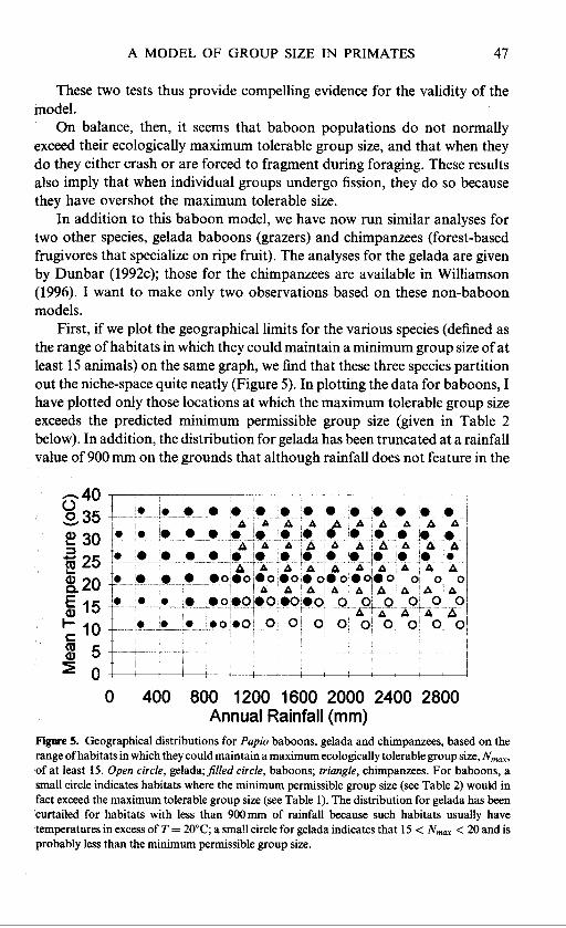
In addition to this baboon model, we have now run similar analyses for two other species, gelada baboons (grazers) and chimpanzees (forest-based frugivores that specialize on ripe fruit). The analyses for the gelada are given by Dunbar (1992~); those for the chimpanzees are available in Williamson (1996). I want to make only two observations based on these non-baboon models.

First, if we plot the geographical limits for the various species (defined as the range of habitats in which they could maintain a minimum group size of at least 15 animals) on the same graph, we find that these three species partition out the niche-space quite neatly (Figure 5). In plotting the data for baboons, I have plotted only those locations at which the maximum tolerable group size exceeds the predicted minimum permissible group size (given in Table 2 below). In addition, the distribution for gelada has been truncated at a rainfall value of 900 mm on the grounds that although rainfall does not feature in the

40 W 0 35 g! 30 E 25

E 15 10

3 CI

8 20

; 5 5 0

c i I I

0 400 800 1200 1600 2000 2400 2800 Annual Rainfall (mm)

Figure 5. Geographical distributions for Papio baboons, gelada and chimpanzees, based on the range of habitats in which they could maintain a maximum ecologically tolerable group size, N,,,, of at least 15. Open circle, ge1ada;filled circle, baboons; triangle, chimpanzees. For baboons, a small circle indicates habitats where the minimum permissible group size (see Table 2) would in fact exceed the maximum tolerable group size (see Table 1). The distribution for gelada has been curtailed for habitats with less than 900 mm of rainfall because such habitats usually have temperatures in excess of T = 20°C; a small circle for gelada indicates that 15 < N,, < 20 and is probably less than the minimum permissible group size.


48 R. I. M . Dunbar

Table 2. Minimum ecologically permissable group size, N,,, for baboons under different climatic conditions.

Annual temperature ("C)

Rainfall (mm) 0 5 10 15 20 25 30 35

100 300 500 700 900

1100 1300 1500 1700 1900 2100 2300 2500 2700 2900

7 29 38 44 49 53 57 7 29 38 44 49 53 57 7 29 38 44 49 53 57 7 29 38 44 49 53 57 3 13 17 20 22 24 26 2 10 13 15 17 18 19 2 9 11 13 15 16 17 2 8 10 12 13 15 16 1 7 10 11 13 14 15 1 7 9 11 12 13 14 1 7 9 10 12 13 14 1 7 9 10 11 12 13 1 6 8 10 11 12 13 1 6 8 9 11 12 12 1 6 8 9 10 11 12

60 60 60 60 27 20 18 17 16 15 14 14 13 13 13

Note: Values predicted by new version of model based on more realistic climatic constraints (see text).

gelada model, there is a relationship between mean temperature and minimum rainfall in the African weather station database: low rainfall values are only found in high temperature habitats. More importantly, data collated by Hurni (1982) for the Simen area also show that habitats below 1500m in altitude (equivalent to mean temperatures in excess of about 19OC at the latitude of the Simen) do not receive more than about 1OOOmm of rain a year, while habitats at higher altitudes do not receive less than this.

The data show that gelada occur only in cooler habitats (mean ambient temperatures of around 10-15°C), as a result of which there is relatively little overlap in geographical range with baboons (who tend to favour habitats with temperatures in the range 20-30°C). This is a consequence of gelada being restricted by their dietary niche to the high altitude grasslands that currently occur only in habitats over about 1500 m in altitude. Analysis of the impact of changing temperature regimes on the altitudinal distributions of baboons and gelada shows rather nicely how the zonal distributions of these two taxa moves up and down the altitudinal gradient as global temperatures rise and fall (Dunbar 1992d). Similarly, the chimpanzee distribution is a more or less mirror image of that for baboons, but with rainfall being the main factor separating the two taxa. This apparently reflects the chimps' preference for tree-based feeding sites in contrast to the baboons' preference for feeding sites in the shrub/bush layer.



Second, the niche separation between the three taxa can be traced back to the dietary differences between them and the way in which their preferred dietary sources respond to climatic variables. The easiest way to show this is in respect of the gelada and the baboon feeding time equations. When these are reduced to the first two independent variables, they have the form:

h(FGe[) = 5.9 - 0.6 h ( T ) - 0.9 1n(Q)

ln(FBub) = 6.4 - 0.6 ln(T) + 5.7 ln(Z) (2)

(3) where Fcer and FBub are the percentages of time devoted to feeding by the gelada and the baboon respectively, Tis mean ambient temperature, Q is the protein content of grass (% protein by weight) and 2 is Simpson’s index of the diversity of rainfall across the months of the year. Now, it turns out that, for this set of baboon study sites, both Q and 2 are quadratic functions of T:

1n(Q) = -26.7 + 23.9 ln(T) - 4.8(ln(T))2

ln(2) = -4.9 + 3.2 ln(T) - 0.6(ln(T))2

(4)

( 5 )

(r2 = 0.97) and

(r2 = 0.65). Substituting equations (4) and (5) into equations (2) and (3) yields:

h(FGe[) = 14.2 - 8.0 h ( T ) + 1.5(ln(T))2

ln(FBub) = -22.2 + 17.5 h ( T ) - 3.1(ln(T))2

which are virtual mirror images of each other: in habitats where baboons have to feed a lot, gelada have to feed relatively little, and vice versa. These turn out to have this form because the two taxa’s primary food sources (grass for the gelada, the bush layer vegetation for baboons) respond in diametrically opposite ways to temperature. Grasses (at least of the kind on which gelada feed) are common at low temperatures, whereas bush level cover is common at higher temperatures. Time spent moving behaves similarly due to the fact that inter-patch distance for each vegetation layer is inversely related to vegetation density.

MINIMUM PERMISSIBLE GROUP SIZE

I assume that the minimum permissible group size is determined by the level of predation risk in a given habitat. Primates in general use group size as a key means of deterring predators (van Schaik 1983; Dunbar 1988). In trying to determine how minimum group size relates to environmental variables, we need to identify the key problems that animals encounter with respect to predation.


50 R. I. M . Dunbar

The first point to note is that mortality per se is not necessarily a good guide to the problem that animals face. If group size is the animals’ response to predation risk, then mortality rates should be constant across habitats (except where animals are prepared to trade up predation risk against other variables in order to be able to survive at all). I therefore assume that animals adjust the minimum size of group they are prepared to live in so that predation risk is equilibrated (to some roughly constant low level) across habitats.

Cowlishaw (1993) found that, in a Namibian baboon population, the degree of cover was the most important factor influencing both the risk of exposure to predator attack and the animals’ nervousness. Similarly, Rasmussen (1983) found that baboons in southern Tanzania were more likely to bunch and to act nervously during travel at those times of year when the level of vegetation cover made it difficult for them to see stalking predators, while Altmann & Altmann (1970) found that both alarms and actual predator attacks in their Kenyan baboon population were concentrated in wooded areas. Equally, however, baboons may be nervous in very open areas when they are far from trees and other suitable refuges (baboons: Byrne 1981; gelada: Dunbar 1989). This suggests that, for baboons at least, predation risk may be positively related to the density of low level cover (e.g. ground and bush layers), but negatively related to the density of large trees that can function as refuges.

Usable data on tree and bush level cover are not available for most of these sites. I therefore used my own data on the percentage of ground surface with tree and bush level cover at nine sites in eastern Africa (see Dunbar 1992a, with an additional Ugandan forest site sampled by Louise Barrett) and derived regression equations relating each of these two variables to fundamental climatic variables. The best-fit equations are:

’

ln(B) = -2.072 + 1.811 ln(T)

E = 86.28 - 14.078V

( r2 = 0.36)

( r2 = 0.85)

where B is the percentage of ground covered by bush/shrub layer vegetation and E is the percentage of ground covered by tree layer vegetation.

I used these equations to calculate tree and bush cover indices for each of the habitats in the sample, and then regressed the minimum observed group size for each population against these values. This yielded the following best-fit equation:

ln(Nmh) = 2.67 - 0.23 ln(E) + 0.202 ln(B) (6)

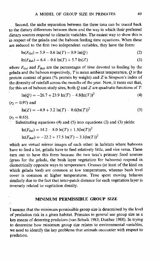
( r2 = 0.516, N = 33, P < 0.05). The distribution in Figure 6 shows quite clearly that the minimum group size gets larger as the level of bush cover



Figure 6. Minimum group sizes for individual baboon populations plotted against percentage of tree and bush level cover for each habitat. Group size increases as the density of bush cover increases and decreases as the density of tree cover increases.

increases (increased risk of unseen predator attack) and the level of tree cover declines (reduced availability of refuges).

If we use equation (6) to determine minimum permissible group sizes, we obtain the distribution given in Table 2. (Once again, I show the data for combinations of rainfall and temperature only, and use these variables to estimate habitat-specific values of Z, V, B and E.) Comparison of Tables 1 and 2 reveals that the minimum permissible group size exceeds the maximum tolerable group size in some habitats, especially those character- ized by less than about 400mm of rainfall and temperatures below about 15OC. Baboons are prevented from occupying these habitats except where micro-habitat conditions (e.g. riverine forest) allow them to reduce the minimum group size or increase the maximum.

COGNITIVE CONSTRAINTS

The final component of the linear programming model is the constraint imposed on group size by the species’ cognitive abilities. This constraint is derived directly from the ‘Machiavellian Intelligence’ hypothesis for primate brain size (Byrne & Whiten 1989). This argues that the principal selection pressure promoting the evolution of large brain size in primates has been the need to integrate and function effectively within increasingly large and tightly bonded social groups. The issue here is not simply creating large loosely structured aggregations. Primate groups are very tightly bonded structures whose coherence through time depends on the acquisition and


52 R. I. M . Dunbar

exploitation of social knowledge about other group members. As a result, primate social groups differ in a number of important ways from those of other species. One of these is the complexity of their coalitions. Harcourt (1989; Harcourt & de Waal 1992) has argued that the coalitions of higher primates differ from those of other species in both their use of third parties and their temporal structure (primate coalitions are commonly established well in advance of the circumstances under which they are needed). These observations suggest that primates are able to acquire and make use of social knowledge about how other individuals behave that is based on deeper insights into others’ mental worlds.

There are two corollaries to this claim. One is that the level of social complexity that one might expect from a species will increase with increasing brain size. This has in fact been shown to be true, both for the use of tactical deception (Byrne 1993) and the use of tactics that undermine the effects of linear dominance hierarchies (Pawlowski & Dunbar 1996). The second is that as the number of individuals that an animal has to keep track of increases, so the cognitive demands on it will increase, and thus demand proportionately larger brains with which to compute social spaces and animals’ trajectories within them.

Note that the issue here is not simply remembering who-is-who in a large group, but rather remembering who-is-friends-with-who, constantly updat- ing this knowledge as friendships change through time and, finally, using this knowledge in building and servicing one’s own friendships and alliances. Prima facie evidence in support of this claim comes from the finding that, in primates, group size does correlate with brain size (Dunbar 1992d, 1995; Barton & Purvis 1995). In both these cases, it seems that it is neocortex size that is crucial (see Barton & Purvis 1995). This is not too surprising, since it is the disproportionate growth of the neocortex that has largely been responsible for the increases in total brain size during primate evolution (Stephan 1972; Passingham 1982).

These findings thus suggest that there is ultimately a cognitive limit to the size of group that a particular species can exhibit. The issue is not that large groups are impossible but that they are much harder to hold together, so that any centrifugal forces that might exist (foraging competition, patch size constraints, harassment) will tend to encourage their dispersal. Such groups will thus tend to fragment rather easily. We do not at present know exactly what the cognitive constraint is. We know only that there is a relationship between mean group size and brain size in primates. Presumably, the information-processing constraint imposed by neocortex size must act via maximum group size. However, we cannot at present identify what this is, since the observed maximum group sizes are likely to be confounded by ecological considerations.



There is, in addition, a further reason for supposing that the relationship between brain size and group size is more complex. Kudo et al. (in preparation) have examined grooming clique sizes in anthropoid primates and shown that these also correlate with relative neocortex size. Grooming cliques are the foundations for coalitions in primate groups, and we suspect that at least part of the constraint may reflect the number of coalitions partners whose conflicting interests can be managed simultaneously. Grooming clique size turns out to be a very tight linear function of group size in anthropoid primates. One plausible interpretation of this is that, as group size increases, so proportionately larger coalitions are needed to buffer individuals against the stresses and strains of living in such large groups.

DISCUSSION

The burden of these analyses is to show that we can define a set of equations that constrain quite tightly the range of group sizes that a given primate species can occupy. These group sizes are habitat-specific and reflect an individual species’ ecological niche adaptations. Figure 1 plots the actual values generated by the baboon systems model for populations living in habitats with a mean annual temperature of 25OC (approximately the centre of the baboon’s thermal zone). I have plotted the cognitive group size as that used in the analysis of neocortex size by Dunbar (1992b). It is therefore necessary to add the rider that this is almost certainly too low: it represents the mean group size not the cognitive maximum group size. It is important to be aware that this is very much a progress report. We are still very much engaged in developing the basic models and further refinements in parameter values and equations can be expected as we learn more about how the animals behave.

Nonetheless, given that we can proceed in this way, three important points follow.

One is that the model as I have presented it is underpinned by conventional optimality considerations. We should be able to identify the limiting processes in the animals’ ecological world that give rise to these group size distributions. Indeed, these optimal solutions to conventional ecological and physiological problems are, in a very real sense, assumptions of the model. We should be able to test these directly by further field work. In many respects, the value of modelling exercises of this kind is to draw our attention to the key processes involved.

A second point arises from the fact that groups are the context in which animals play out their social and reproductive strategies. Their decisions on which strategies to pursue are influenced by the costs and benefits of the


54 R. I. M . Dunbar

options available to them. Not only may the options themselves be determined by the size and composition of their groups (you can only choose to form an alliance with a sister if you have sisters living with you), but also the very costs and benefits that weight those strategies are a product of the demography of the group. Thus, once we know group size, a number of other things follow in a fairly straightforward way (Dunbar 1993b). I shall confine myself to just one example here.

It turns out that, for most primate species, the number of males in a group is a function of the number of females in the group (Dunbar 1988). In most cases, this is a direct consequence of an optimization problem being solved by the males in the population. The problem was originally identified by Emlen & Oring (1977) as one of monopolizing reproductive females. Dunbar (1988) has shown that, in primates at least, a male’s ability to keep other males away from a group of females (so as to maintain a one-male group) depends on a combination of the size of the female group (a direct reflection of the ecological constraints on group size) and the reproductive synchrony among the females. (Srivastava & Dunbar [in press] have since been able to show that the distance males have to travel to find another female group [the search time in conventional optimal foraging terminology] is also an important consideration.) Thus, the choice between female- defence polygyny and conventional mate-defence promiscuity turns out to be a direct consequence of the way demographic and lifehistory variables weight the costs and benefits of mate defence for males.

Once males are in a multimale group, further consequences follow. Cowlishaw & Dunbar (1991) have shown that the dominant male’s ability to monopolize matings within a multimale group is a negative function of the number of males in the group (and hence the pressure from rivals). In fact, there appears to be a crucial threshold at four males: with a small number of competitors in the group, the dominant male can command a disproportionate share of the matings (and, indeed, conceptions), but once there are more than four males it becomes increasingly difficult for him to do so.

In part, the dominant male’s problem reflects the extent to which females can exert an influence on the situation through female choice. This, in turn, is partly a reflection of levels of sexual size dimorphism (something which varies considerably not just between species, but also within species in response to environmental parameters: for baboons, see Dunbar 1990). The larger males are relative to females, the more valuable they are as allies in any situation where power is a function of physical size. Although females have to balance a male’s size-dependent value as an ally against the value of longer-lasting alliances formed with female relatives (Dunbar 1988, 1993b), there will inevitably be a point at which the power-asymmetry offered by large males outweighs the benefits offered by female relatives through kin selection.



As a result, group composition, male mating strategies and female social strategies should be a straightforward function of group size and other ecological factors. However, in contrast to the species-specific socio- ecological models of the 1970s, the important lesson from these analyses is that these variables may be expected to vary from one population to another within a species. Preliminary analyses (Dunbar 1993b) suggest that this simple deterministic model yields outcomes for these social variables that bear a rather complex relationship to climatic variables. Although the relationships involved are all causally deterministic, non-linear elements in the equations generate what appear superficially to be chaotic behaviour when carried through into further layers of equations.

Finally, given that we can define both demographic and behavioural aspects of a species’ behaviour in this way, one obvious implication is that we can do the same for extinct species. The constraints lie only in the precision of our knowledge about the climatic parameter values for palaeoenvironments, body weights for extinct species and their dietary niches. Of these, only the latter remains genuinely problematic, although even in this respect tooth shape and wear patterns (Kay & Covert 1984) and the trace element content of fossil bone (e.g. Lee-Thorp et al. 1989) are beginning to elucidiate matters. Significant advances have been made during the past decade in determining palaeoclimates from both faunal and vegetational assemblages and it is possible to specify with some degree of confidence the likely rainfall and temperature values by using modern habitats with comparable faunal or floral profiles (e.g. Vrba 1988). Similarly, it is now possible to estimate body weights with considerable accuracy from bone fragments: thanks mainly to general physical principles, the cross-sectional dimensions of weight-bearing bones provide an accurate estimate of the weight they carried in life (e.g. Martin 1990). Given this, it should be possible to say quite a lot about the population demography and behavioural ecology of individual populations of fossil taxa, at least so long as they belong to the same dietary grade as a living taxon. Preliminary attempts to do so have been carried out for fossil papionines (Dunbar 1991) and fossil theropithecines (Dunbar 1993a) with some success.

In addition to predicting how a taxon might have behaved at a given site, we can use the model in reverse to explore the likely reasons why a species went extinct. By using the model to predict group size at fossil sites where they are known not to have occurred or at different time horizons within a site, we may be able to show why a species went extinct.

In sum, the approach adopted here holds out significant hope for building a model that allows us both to predict the form and structure of species’ socio-ecological systems and to explore aspects of that species’ biogeography and evolutionary history postdictively as well as predictively.


56 R. I . M . Dunbar

In other words, not only may we be able to account for the species’ past history, but we may also be able to predict what the consequences of major habitat or climatic change may be for the species’ distribution and future survival. By simultaneously building top-down (i.e. systems models of the kind described here) and bottom-up (i.e. more conventional optimization models), we may be able to produce a very securely constructed general theory of primate social systems.

REFERENCES

Altmann, J. 1980: Baboon Mothers and Infants. Cambridge (MA): Harvard University Press. Altmann, S.A. & Altmann, J. 1910: Baboon Ecology. Chicago: University of Chicago Press. Barton, R.A. & Purvis, A.J. 1995: Primate brains and ecology: looking below the surface. In

Proceedings of XIVth Congress of the International Primatological Society, Strasburg. Brain, C . 1990: Spatial usage of a desert environment by baboons (Papio ursinus). Journal of

Arid Environment 18, 61-73. Byme, R.W. 1981: Distance vocalisations of Guinea baboons (Papio papio) in Senegal: an

analysis of function. Behaviour 78, 283-312. Byrne, R. 1993: The Thinking Ape. Oxford: Oxford University Press. Byme, R.W. & Whiten, A. (eds) 1989: Machiavellian Intelligence. Oxford: Oxford University

Cowlishaw, G. 1993: Trade-offs Between Feeding Competition and Predation Risk in Baboons.

Cowlishaw, G. & Dunbar, R.I.M. 1991: Dominance rank and mating success in male primates.

Dunbar, R.I.M. 1988: Primate Social Systems. London: Chapman & Hall. Dunbar, R.I.M. 1989: Social systems as optimal strategy sets: the costs and benefits of sociality.

In Comparative Socioecology (ed. V. Standen & R. Foley), pp. 131-150. Oxford Blackwell Scientific.

Dunbar, R.I.M. 1990: Environmental determinants of intraspecific variation in body weight in baboons (Papio spp.). Journal of Zoology, London, 220, 157-169.

Dunbar, R.I.M. 1991: Functional significance of social grooming in primates. Folia Primatologica 51, 121-131.

Dunbar, R.I.M. 1992a. Time: a hidden constraint on the behavioural ecology of baboons. Behavioural Ecology and Sociobiology 31, 35-49.

Dunbar, R.I.M. 1992b. Neocortex size as a constraint on group size in primates. Journal of Human Evolution 20, 469-493.

Dunbar, R.I.M. 1992c. A model of the gelada socioecological system. Primates 33, 69-83. Dunbar, R.I.M. 1992d. Behavioural ecology of the extinct papionines. Journal of Human

Evolution 22, 401-421. Dunbar, R.I.M. 1993a. Socioecology of the extinct theropiths: a modelling approach. In

Theropithecus: The Rise and Fall of a Primate Genus (ed. N.G. Jablonski), pp.465-486. Cambridge: Cambridge University Press.

Dunbar, R.I.M. 199313. Ecological constraints on group size in baboons. Physiology & Ecology, Japan 29, 221-236.

Dunbar, R.I.M. 1995: Neocortex size and group size in primates: a test of the hypothesis. Journal of Human Evolution 28, 281-296.

Dunbar, R.I.M. & Dunbar, P. 1988: Maternal time budgets of gelada baboons. Animal Behaviour 36, 970-980.

Press.

PhD thesis, University of London.

Animal Behaviour 41, 1045-1056.



Dunbar, R.I.M. & Shaman, M. 1984 Is social grooming altruistic? Zeitschrgt fCr Tierpsychologie 64, 163-173.

Emlen, S.T. & Oring, L. 1977: Ecology, sexual selection and the evolution of mating systems. Science 197, 215-223.

Harcourt, A.H. 1989: Social influences on competitive ability: alliances and their consequences. In Comparative Socioecology (ed. V. Standen & R. Foley), pp. 223-242. Oxford: Blackwell Scientific.

Harcourt, A.H. & de Waal, F. (eds) 1992: Coalitions and Alliances in Humans and Other Animals. Oxford: Oxford University Press.

Humi, H. 1982: Climate and the Dynamics of Altitudinal Belts from the Last Cold Period to the Present Day. (Simen Mountains-Ethiopia, Vol. 11) Bern: University of Bern Geographical Institute.

Kawamuto, Y., Shotake, T., & Nozawa, K. 1982: Genetic differentiation among three genera of Family Cercopithecidae. Primates 23, 272-286.

Kay, R.F. & Covert, B. 1984: Anatomy and behaviour of extinct primates. In Food Acquisition and Processing in Primates (ed. D.J.Chivers, B. Wood & A. Bilsborough), pp. 467-508. New York Plenum Press.

Lee-Thorp, J.A., van der Merwe, N.J. & Brain, C.K. 1989: Isotopic evidence for dietary differences between two extinct baboon species from Swartkrans. Journal of Human Evolution 18, 183-190.

Martin, R.D. 1990: Primate Origins and Evolution. London: Chapman & Hall. Mount, L.E. 1979: Adaptation to Thermal Environment. London: Arnold. Passingham, R. 1982: The Human Primate. San Francisco: Freeman. Pawlowski, B.B. & Dunbar, R.I.M. 1996: Neocortex size, social skills and mating success in

male primates. (Submitted) Rasmussen, D.R. 1983: Correlates of patterns of range use of a troop of yellow baboons (Papio

cynocephalus). 11. Spatial structure, cover density, food gathering, and individual behaviour patterns. Animal Behaviour 31, 834-856.

Sear, R. 1994 A Quantitative Analysis of Gibbon behavioural Ecology. MSc thesis, University College London.

Shaman, M. & Dunbar, R.I.M. 1982: Observer bias in selection of study group in baboon field studies. Primates 23, 567-573.

Srivastava, A. & Dunbar, R.I.M. (In press) The mating system of hanuman langurs: a problem in optimal foraging. Behavioural Ecology and Sociobiology.

Shotake, T., Nozawa, K., & Tanabe, Y. 1977: Blood protein variations in baboons. I. Gene exchange and genetic distance between Papio anubis. Papio hamadryas and their hybrids. Japanese Journal of Genetics 52, 223-237.

Stephan, H. 1972: Evolution of primate brains: a comparative anatomical investigation. In Functional and Evolutionary Biology of Primates (ed. R. Tuttle), pp. 155-174. Chicago: Aldine- Atherton.

van Schaik, C.P. 1983: Why are diurnal primates living in groups? Behaviour 87, 120-144. Vbra, E.S. 1988: Late Pliocene climatic events and hominid evolution. In Evolutionary History

of the 'Robust' Australopithecines (ed. F.Grine), pp. 183-238. Albany: SUNY Press. Wernstedt, F.L. 1972: World Climatic Data. New York Climatic Data Press. Williamson, D. 1996: Modelling the Socioecology of Early Hominids. PhD thesis, University of

Wrangham, R.W. 1980: An ecological model of female-bonded primate groups. Behaviour 75,

Wrangham, R.W. 1987: Evolution of social structure. In Primate Societies (eds. B.B.Smuts, D. Cheney, R. Seyfarth, R.W. Wrangham & T.T. Struhsaker), pp. 282-295. Chicago: Chicago University Press.

London.

262-300.


Determinants of Group Size in Primates: A General Model · 2020-05-14 · The principal analysis...

Documents

Transcript of Determinants of Group Size in Primates: A General Model · 2020-05-14 · The principal analysis...