Sustainable Upland Farm Businesses (1): Exploring

determinants of efficiency among England’s upland

farms

Janet Dwyer1 and Mauro Vigani1

1University of Gloucestershire - CCRI

Contributed Paper prepared for presentation at the 90th Annual Conference of the

Agricultural Economics Society, April 4-6 2016, Warwick University, Coventry, UK

Copyright 2016 by author(s). All rights reserved. Readers may make verbatim copies of this document for

non-commercial purposes by any means, provided that this copyright notice appears on all such copies.

1

Sustainable Upland Farm Businesses (1): Exploring determinants of efficiency among England’s upland farms

Janet Dwyer1 and Mauro Vigani1 1University of Gloucestershire - CCRI

Abstract

This paper represents the start of a research programme to investigate in detail the economics of English upland farming, in order to pursue greater economic, environmental and social sustainability in future. The Farm Business Survey sample of farms in the English LFA is analysed, examining economic performance over 4 years (2010 to 2013), looking for potential determinants of efficiency. The analysis examines technical efficiency as a first indicator, and analyses data for the 263 LFA grazing livestock farms in the dataset. A stochastic frontier approach is used to test hypotheses concerning whether farm scale, and/or various indicators of farming intensity, CAP subsidy and risk management, have significant influence upon performance. The results highlight some of the challenges in identifying and applying suitable indicators and suggest that the LFA may best be analysed by differentiating between higher-altitude and lower-lying farms, as the economic characteristics of these two groups are distinct. Within these groups we identify specific strategies as potentially significant, including early recruitment of ewe lambs into breeding and the sale of wool, as well as diversification off the holding, for lower lying farms; while agri-environment support and extensification appear influential among the higher-altitude group. Planned next steps include applying meta-frontier techniques; also analysing for determinants of profitability; and building a discussion and exchange forum with farmers and other stakeholders, through the Uplands Alliance, to maximise the value of these analyses via a wider community of learning.

1. Introduction: context and aim of the paper

For many years now, the Farm Business Survey analysis of farming in England’s Less Favoured Areas has suggested that the majority of hill and upland farms in the country struggle to cover their costs, year on year, and depend significantly for their survival upon continuing high levels of government subsidy from both Pillars of the CAP (Harvey and Scott, 2011; 2012; 2013; 2014; 2015). Yet at the same time, these analyses suggest that there can be significant differences in performance between farms in these areas, with the most efficient businesses making reasonable net incomes and agricultural business incomes (i.e. net of subsidy), even in relatively poor years (ibid). The annual survey reports offer few clues as to what factors appear to underlie these differences. Expert commentators, advisers and farmers themselves suggest different tactics for improving profitability and/or viability, with some believing that growth – in land and in business scale – is the only way to enhance returns, while others encourage income

2

diversification and/or extensification (cutting costs to a minimum) as more promising strategies for resilience and survival (e.g. Harvey and Scott, 2013; Dwyer et al, 2015; Eblex, 2014; Jones, 2015).

The aim of the paper is to use the detailed farm-level dataset of Defra’s Farm Business Survey since 2010 to analyse in greater depth, the determinants of farming efficiency of uplands LFA Grazing Livestock Farms. Through this, it is hoped to stimulate further knowledge exchange with farmers, policy makers and other upland stakeholders in an effort to promote more economically, environmentally and socially resilient and successful farming in these areas, in the future. For this purpose, we develop and compare two hypotheses drawn from the current literature.

The first hypothesis is built on the common assumption that the most successful upland farms – therefore those which appear most technically efficient - are those with bigger dimensions (as was identified by Harvey and Scott in 2013). This is in line with a notion of economies of scale applying to England’s upland farms. Based on this assumption, the first hypothesis that we would seek to test is:

H1: Upland farms’ efficiency increases with farm business size or the area of land farmed.

The second hypothesis derives from a consideration of market and policy challenges faced by farms in the uplands, over the last decade. These challenges are linked to market liberalisation, increased price volatility and the full decoupling of single payment subsidies in 2005, as well as the increased targeting of support to those upland farms delivering environmental services, through Environmental Stewardship (Silcock et al., 2012).

In responding to these combined challenges, we suggest that some farms may instead be pursuing economies of scope, as a tactic to enhance performance. This could mean that some upland farmers have adopted strategies of either agricultural intensification or extensification, and/or greater ‘risk management’, including income diversification. These strategies would also determine different levels of farming efficiency, hence a second hypothesis for testing is:

H2: Intensification, risk management and the type and scale of CAP payments received affect the efficiency of upland farms.

2. Conceptual framework

In order to estimate the impact of the different factors determining the efficiency of upland farming, we use a stochastic frontier (SF) analysis. The SF analysis is a two-step simultaneous estimation: first, the estimation of the SF production function, and, second, the estimation of the inefficiency model.

The SF model is based on the theory that no economic agent (company or farm) can exceed the ideal “frontier" of the maximum amount of output that can be obtained from a given allocation of inputs – so, a measure of relative technical efficiency in using the factors of production. Any

3

deviations from this extreme are seen as representing an individual farm’s relative inefficiency in allocating and using inputs. Note that for this calculation, the total value of output is measured net of CAP subsidies – so, assessing the value of the agricultural outputs alone.

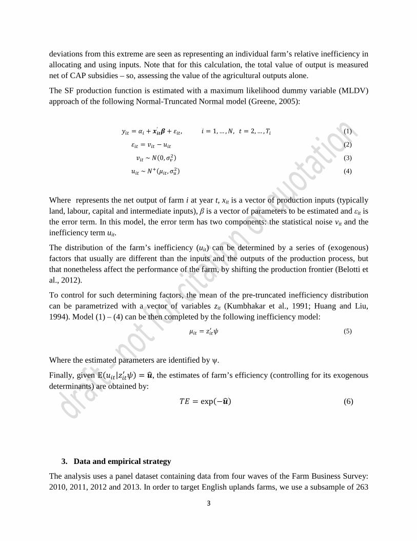
The SF production function is estimated with a maximum likelihood dummy variable (MLDV) approach of the following Normal-Truncated Normal model (Greene, 2005):

𝑦𝑖𝑖 = 𝛼𝑖 + 𝒙𝒊𝒊’ 𝜷 + 𝜀𝑖𝑖 , 𝑖 = 1, … ,𝑁, 𝑡 = 2, … ,𝑇𝑖 (1) 𝜀𝑖𝑖 = 𝑣𝑖𝑖 − 𝑢𝑖𝑖 (2) 𝑣𝑖𝑖 ~ 𝑁(0,𝜎𝑣2) (3)

𝑢𝑖𝑖 ~ 𝑁+(𝜇𝑖𝑖 ,𝜎𝑢2) (4)

Where represents the net output of farm i at year t, xit is a vector of production inputs (typically land, labour, capital and intermediate inputs), β is a vector of parameters to be estimated and εit is the error term. In this model, the error term has two components: the statistical noise vit and the inefficiency term uit.

The distribution of the farm’s inefficiency (uit) can be determined by a series of (exogenous) factors that usually are different than the inputs and the outputs of the production process, but that nonetheless affect the performance of the farm, by shifting the production frontier (Belotti et al., 2012).

To control for such determining factors, the mean of the pre-truncated inefficiency distribution can be parametrized with a vector of variables zit (Kumbhakar et al., 1991; Huang and Liu, 1994). Model (1) – (4) can be then completed by the following inefficiency model:

𝜇𝑖𝑖 = 𝑧𝑖𝑖′ 𝜓 (5)

Where the estimated parameters are identified by ψ.

Finally, given 𝔼(𝑢𝑖𝑖|𝑧𝑖𝑖′ 𝜓) = 𝒖�, the estimates of farm’s efficiency (controlling for its exogenous determinants) are obtained by:

𝑇𝑇 = exp(−𝒖�) (6)

3. Data and empirical strategy

The analysis uses a panel dataset containing data from four waves of the Farm Business Survey: 2010, 2011, 2012 and 2013. In order to target English uplands farms, we use a subsample of 263

4

farms contained in the FBS. These farms are classified as LFA Grazing Livestock Farms, each one having more than two thirds of its total SO standard output coming from cattle, sheep and other grazing livestock; and 50% or more of its total area in the LFA.

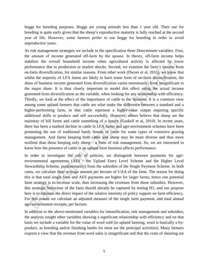
The productivity of uplands farms is represented by a Cobb–Douglas stochastic production frontier, estimated through the following MLDV “true” fixed effects (TFE) time-varying model (Greene, 2005):

𝑙𝑛𝑦𝑖𝑡 = ɑi + 𝛽1 𝑙𝑛𝐿𝑎𝑏𝑜𝑢𝑟𝑖𝑡 + 𝛽2 𝑙𝑛𝐿𝑎𝑛𝑑𝑖𝑡 + 𝛽3 𝑙𝑛𝐴𝑠𝑠𝑒𝑡𝑠𝑖𝑡 + 𝛽𝑛 ∑𝑙𝑛𝐼𝑛𝑡𝑒𝑟𝑚𝑒𝑑𝑖𝑎𝑡𝑒 𝑖𝑛𝑝𝑢𝑡𝑠𝑖𝑡 + 𝑣𝑖𝑡 − 𝑢𝑖𝑡 (7)

Where 𝑦𝑖𝑡 is the value of agricultural output of farm i at time t and intermediate inputs are veterinary medical costs, and machinery running costs.

The TFE model has some important advantages over other time-varying SF models. It allows us to solve the problem of time invariant unobservable factors (which are unrelated to the production process but can affect the output) through unit-specific intercepts (ɑi). While other time-varying models estimate the same intercept (ɑ) across all the productive units generating a mis-specification bias in the inefficiency term uit, the TFE model disentangles the time-varying inefficiency from the unit specific time invariant unobserved heterogeneity, reducing the bias in uit.

The inefficiency model contains the determinants potentially affecting the farm efficiency and it is defined by the equation:

𝑢𝑖𝑖 = δ 0 + ∑ δ𝑛𝑘𝑛=1 HHC𝑖𝑖 + ∑ δ𝑙𝑘

𝑙=1 Determinants𝑖𝑖 (8)

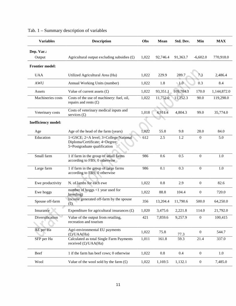
Where HHC are standard head-of-household characteristics (age and education). Our variables of interest to test H1 and H2 are contained in the group of Determinant variables. Descriptive statistics of the variables used in the SF model are presented in Table 1.

To test H1 (whether farm size affects the technical efficiency of upland farms, net of subsidies), we use two binary variables. The first is equal to 1 if the farm falls into the category of “small farms” according to the classification of the FBS, and 0 otherwise. The second one is a similar binary variable, but equal to 1 if the farm falls in the FBS category of “large” farms. These categories appear to be determined on the basis of economic size class, for all FBS farms.

In order to test H2, the Determinant variables include proxies for agricultural intensification, risk management and policies.

To account for agricultural intensification we use the following variables: i) the intensity of lambs per ewe (Lambs/Ewe), which is also a measure of ewes’ productivity; ii) the use of ewe

5

hoggs for breeding purposes. Hoggs are young animals less than 1 year old. Their use for breeding is quite early given that the sheep’s reproductive maturity is fully reached at the second year of life. However, some farmers prefer to use hoggs for breeding in order to avoid unproductive years.

As risk management strategies we include in the specification three Determinant variables. First, the amount of income generated off-farm by the spouse. In theory, off-farm income helps stabilize the overall household income when agricultural activity is affected by lower performance due to production or market shocks. Second, we examine the farm’s income from on-farm diversification, for similar reasons. From other work (Dwyer et al, 2015), we know that whilst the majority of LFA farms are likely to have some form of on-farm diversification, the share of business income generated from diversification varies enormously, from insignificant to the major share. It is thus clearly important to model this effect using the actual income generated from diversification as the variable, when looking for any relationship with efficiency. Thirdly, we look at the effect of the importance of cattle to the business. It is a common view among some upland farmers that cattle are what make the difference between a standard and a higher-performing farm, in that cattle represent a higher-value output requiring specific additional skills to produce and sell successfully. However, others believe that sheep are the mainstay of hill farms and cattle something of a luxury (Gaskell et al, 2010). In recent years, there has been a marked decline in cattle in LFA farms and agri-environment schemes have been promoting the use of traditional hardy breeds of cattle for some types of extensive grazing management. And farms keeping both cattle and sheep may be more diverse and thus more resilient than those keeping only sheep – a form of risk management. So, we are interested to know how the presence of cattle in an upland farm business affects performance.

In order to investigate the role of policies, we distinguish between payments for agri-environmental agreements (AES - the Upland Entry Level Scheme and the Higher Level Stewardship Scheme, predominantly) from the subsidies of the Single Payment Scheme. In both cases, we calculate their average amount per hectare of UAA of the farm. The reason for doing this is that total single farm and AES payments are higher for larger farms; hence one potential farm strategy is to increase scale, thus increasing the revenues from these subsidies. However, this strategic behaviour of the farm should already be captured by testing H1, and our purpose here is to estimate the direct impact of the relative intensity of policy support on farm efficiency. For this reason we calculate an adjusted measure of the single farm payment, and total annual agri-environment receipts, per hectare.

In addition to the above-mentioned variables for intensification, risk management and subsidies, the analysis sought other variables showing a significant relationship with efficiency and on that basis we include a variable for the value of wool sold (in upland farming, wool is basically a by-product, as breeding and/or finishing lambs for meat are the principal activities). Many farmers express a view that the revenue from wool sales is insignificant and that the costs of shearing are

6

rarely recouped from this revenue. So, we were interested to know how selling wool appears related to overall efficiency.

All the variables included in the model are used in their logarithmic form, with the exception of the binary variables.

Efficiency estimations are conducted for the whole sample of upland farms, but also dividing the sample into two groups, for farms located above and below 300m in altitude, to examine how this affects the patterns emerging. The altitude of farms may induce different strategies in allocating inputs, related to the fact that at higher altitudes land is much less fertile and less productive, so different tactics may be needed and different business strategies better suited to these harsher conditions.

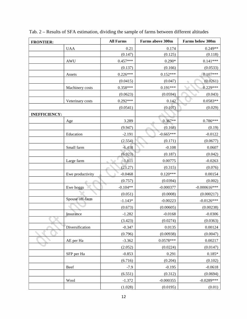
4. Results and discussion

Table 2 shows the results of the SF model. In the first column the results cover the whole sample of upland farms included in the FBS dataset for the period 2010-2013. In the second and third columns the sample of upland farms is divided into those farms located above and below 300m in altitude, respectively, over the same period. This discussion compares the patterns revealed in the analysis with our qualitative understanding of upland farmer opinions, experiences and concerns in England, drawn from a number of recent, previous studies (Dwyer et al, 2015; Gaskell et al, 2010, Clothier and Finch, 2009).

Firstly, we note that the variables used for estimating the production frontier are all of the expected sign (so, positively linked to the outcome) and the majority appear statistically significant. Increasing levels of agricultural land (UAA), assets (the value tied up in current stock and machinery), labour force, machinery and veterinary input costs are each positively associated with higher agricultural output, for the group of upland farms located below 300m (i.e. those which should have slightly more productive land holdings). However, the output value of the group of farms above 300m is significantly related only to their agricultural land area and machinery costs (so, labour force and veterinary costs have insignificant relationships to production value – probably reflecting the lower labour and veterinary costs of these production systems more generally).

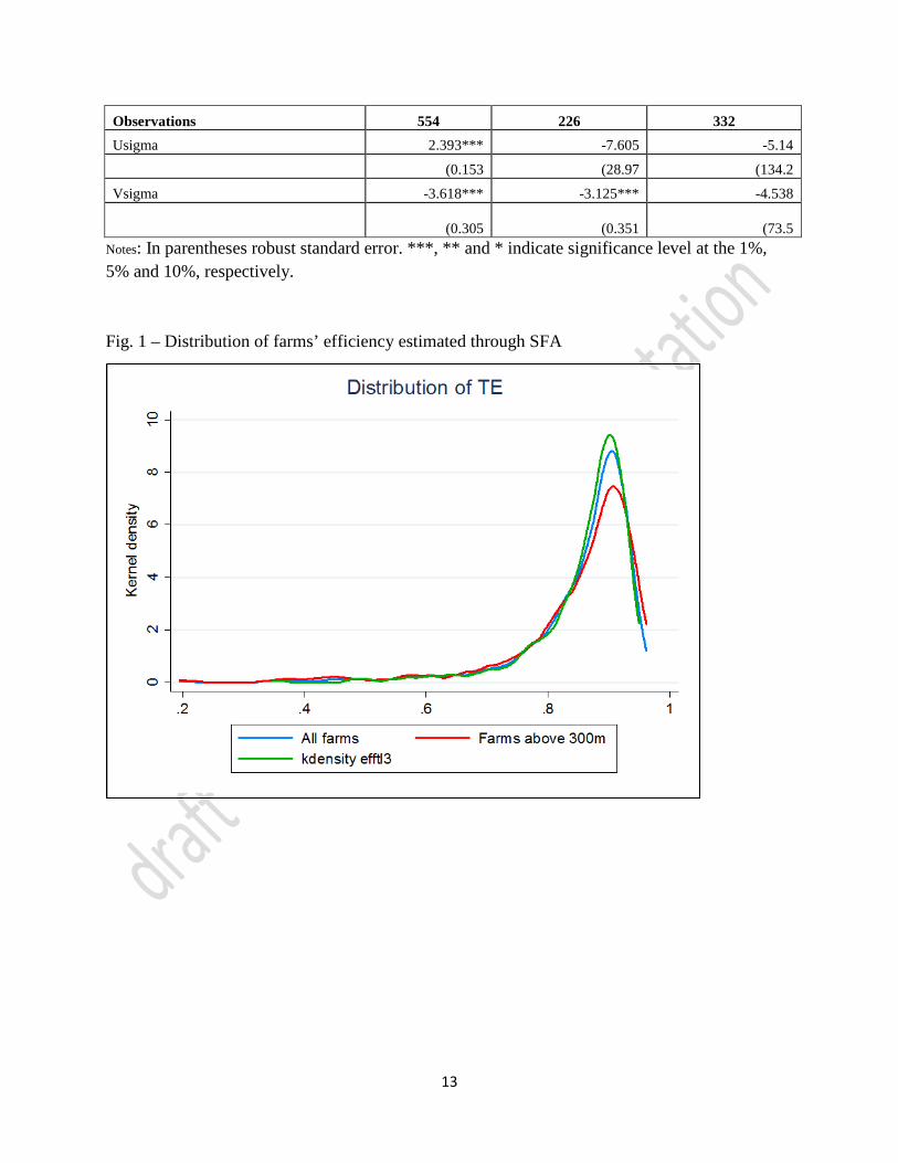
Interestingly, UAA does not appear significant in influencing output when the whole sample is analysed together, nor for the higher-altitude farms alone, which tends to suggest that the absolute performance levels of the two groups and their relationships to the area farmed are actually quite different. In order to compare the overall level of efficiency between upper and lower-lying farms, we obtained estimates of the efficiencies through Eff = exp(-û). The distributions of the efficiencies of the whole sample and of the farms above and below 300m are shown in Figure 1. The distributions are similar, all with negative skewness, but the figure clearly shows that lower-lying farms are, on average, more technically efficient than higher-altitude farms, as would be expected, given the variation in land quality. This presents a strong

7

case for dealing separately with the interpretation of our dataset, as between lower and higher-altitude farms within the group as a whole. And indeed, the determinant variables’ relationships to inefficiency in Table 2 show important differences between farms above and below 300m.

H1 is not confirmed by the result of the binary variable “Large farm” for the whole dataset, which could suggest that larger farms (in respect of scale of business - ESU) are associated with higher inefficiency. However, some caution is necessary here, as the share of these farms in the total is relatively small – under 10% of the sample - so we are dealing with small numbers, in looking for any relationship. By contrast, ‘small farms’ classified by business scale account for more than half of the total FBS LFA population. Here, we see no clear relationship between business scale and efficiency, using this binary approach, either for the whole dataset or for the two altitude-defined groups taken separately.

In columns 2 and 3 (i.e. when the farms are analysed separately according to altitude), the frontier model shows a significant and positive effect of larger UAA on farm output for the lower-lying farms only. So, larger farms (by area) produce a higher value of output, as would be expected. But we cannot say whether UAA affects relative efficiency from this data, as we have used it as a variable to estimate the frontier. More work is necessary to seek a method which could more adequately investigate the influence of farm size in UAA, upon farm performance.

Concerning H2, we begin by looking at the variables for intensification. The positive and significant sign of the ewe productivity variable in the sample of farms on the higher altitude land suggests that having more lambs per ewe is not a good strategy to increase farm efficiency in these most marginal areas. This result would appear to confirm expert and farmer opinions that ‘true hill farms’ operating on the poorest land should not attempt to seek high lambing percentages. By contrast, the practice of using young ewe hoggs for breeding seems successful in terms of production-factor efficiency, among both higher and lower-lying farms. However, it is worth noticing that the coefficients are quite small, suggesting that the gains in efficiency from breeding with ewe hoggs are modest. This again would appear to be consistent with accepted wisdom in respect of limits to production efficiency. Many farmers believe that the biggest challenge to LFA livestock farming is the high costs of keeping stock through the winter when they require feeding, but grass is not growing. For those ewes carrying lambs, this cost represents an investment in the following year’s income from lamb sales, but for ewe hoggs which are not in lamb, it would represent an investment for the longer term, over 2 years, which is more costly.

Among the variables for risk management, on-farm diversification strategies seem to have an insignificant efficiency effect. However the results suggest that on lower-lying farms, a significantly higher level of efficiency is found on farms with additional income coming from off-farm work by the spouse. In higher-altitude farms neither of these variables appears significantly related to greater technical efficiency.

In respect of the influence of cattle in the business mix, the relationship was not found to be significant when modelled in this simple way (using a dummy variable for yes/no). We believe it would be worth seeking an improved indicator of the influence of cattle, to explore this further.

8

Also, to examine diversification effects, some differentiation of the sources of income between tourism, sport or other outputs could also be very useful.

Regarding policies and subsidies, no relationship is apparent between the relative level of support from the single farm payment and farms’ technical efficiency. However, the coefficient of agri-environment payments turns significantly positive in the case of farms above 300m (so, the higher the AES payment, the lower the technical efficiency). This seems logical in that farms which enter HLS are anticipated to forego some level of agricultural output in order to prioritise environmental outputs – an extensification which represents less-than-efficient performance, in economic terms, order to increase environmental effectiveness, for which they receive compensation through the scheme.

Finally, selling wool seems to improve significantly the efficiency of those LFA farms located below 300m, although for all farms, the sign of the relationship is positive but the relationship is not strong enough to be significant. This would appear to suggest that selling wool is making a positive contribution to a more efficient use of farming resources, particularly for lower-lying (more productive) farms.

5. Conclusions and next steps

These are emerging results of an analysis which we plan to take further, as we become more experienced in using the FBS dataset to good effect. As such, the tentative relationships suggested in this paper should be viewed as starting points, rather than significant conclusions, in respect of our basic hypotheses. We suggest that the most interesting points are:

• That farms above and below the 300m altitude mark appear to operate systems with different characteristics which require separate analysis

• That no strong linkage between farm business size and technical efficiency is yet apparent – but we accept this needs further probing in view of the less-than-ideal initial approach to this question that we have used

• That some relationships appear to confirm practitioner views about LFA farms’ limited scope for increasing productivity, and the significant cost of keeping non-productive adult sheep

• That income diversification through working off-farm appears to have a positive impact upon efficiency, in contrast to one popular narrative which suggests that dividing a family’s time and attention between farming and another business will mean they ‘take their eye off the ball’ in respect of the quality of their farm operations

• That, again contrary to some perceptions within the sector, wool sales can make a positive contribution to the overall efficiency of the farm business.

These are first-cut findings which we plan to feed into further work to interrogate and understand the dataset and what it can tell us about LFA farming performance. Key next steps include the following:

9

• To re-run the analysis using some more refined indicators, in respect of some variables and considering other variables as suggested in discussions at the conference;

• We will consider making an analysis of efficiency using the alternative ‘meta-frontier’ approach which has been favoured by others as producing more accurate assessments (O’Donnel et al., 2008);

• We will make an analysis of the effect of variables such as are examined here, upon farm profitability, to see if this shows up significant differences between farm performance measured in these two ways. Ultimately, it should be profitability over the medium term which underpins farm business sustainability and this is not quite the same as efficiency;

• Once we feel we have sufficient material of interest, we will share it with the emerging farmer and stakeholder groups convened as part of the Uplands Alliance, to examine sustainable farm business models for the uplands. Our work is intended as a stimulus to alternative and complementary practical and applied thinking, adding to shared understanding, and seeking options for better policy and practice in future.

6. References

Battese, G. E. and Coelli, T. J., 1995. A model for technical inefficiency effects in a stochastic frontier production function with panel data. Empirical Economics. 20: 325–332.

Belotti, F., Daidone, S., Ilardi, G. and Atella, V. (2012). Stochastic frontier analysis using Stata. The Stata Journal, 55(2): 1-39.

Clothier, L., & Finch, F. (2009). The farm practices survey: uplands and other less favoured areas (LFAs) survey report. Defra Agricultural Change and Environment Observatory Research Report No. 16. Dwyer, J, Condliffe, I, Short, C and Pereira, S. (2010) Sustaining marginal areas: the case of the English uplands. RuDI Case Study WP8 report. CCRI, Cheltenham. At www.rudi-europe.net Dwyer, J., Mills, J., Powell, J., Lewis, N., Gaskell, P. and Felton, J. (2015) The State of Farming in Exmoor, 2015. Report to the Exmoor Hill Farming Network. CCRI, Gloucester.

Eblex (2014) Stocktake report 2014. Agricultural and Horticultural Development Board, London.

Gaskell, P., Dwyer, J., Jones, J., Jones, N., Boatman, N., Condliffe, I., Conyers, S., Ingram, J., Kirwan, J., Manley, W., Mills, J., and Ramwell, C. (2010) Economic and environmental impacts of changes in support measures for the English Uplands: An in-depth forward look from the farmer’s perspective, Final report to the Defra Agricultural Change and Environment Observatory programme by the Countryside and Community Research Institute and the Food and Environment Research Agency Central Science Laboratory.

10

Harvey, D. And Scott, C. (2012) Farm Business Survey 2010/2011 Hill Farming in England. Rural Business Research at Newcastle University.

Harvey, D. And Scott, C. (2013) Farm Business Survey 2011/2012 Hill Farming in England. Rural Business Research at Newcastle University.

Harvey, D. And Scott, C. (2014) Farm Business Survey 2012/2013 Hill Farming in England. Rural Business Research at Newcastle University.

Harvey, D. And Scott, C. (2015) Farm Business Survey 2013/2014 Hill Farming in England. Rural Business Research at Newcastle University.

Huang, C. J., and J. T. Liu. 1994. Estimation of a Non-Neutral Stochastic Frontier Production Function. The Journal of Productivity Analysis, 5: 171-180.

Jones, G. (2014) High Nature Value farming in the Northern Upland Chain, European Forum on Nature Conservation and Pastoralism.

Kumbhakar, S. C., S. Ghosh, and J. T. McGuckin (1991). A Generalized Production Frontier approach for estimating the inefficiency in U.S. Dairy Farms. Journal of Business & Economic Statistics 9: 279-286.

O’Donnell, C. J., Rao, D. S. P., Battese, G. E. (2008). Metafrontier frameworks for the study of firm-level efficiencies and technology ratios. Empirical Economics 34, 231–255.

Silcock, P., Brunyee, J. and Pring, J. (2012). Changing livestock numbers in the UK Less Favoured Areas – an analysis of likely biodiversity implications. Report for the Royal Society for the Protection of Birds.

11

Tab. 1 – Summary description of variables

Variables Description Obs Mean Std. Dev. Min MAX

Dep. Var.: Output Agricultural output excluding subsidies (£) 1,022 92,746.4 91,363.7 -6,602.0 770,918.0

Frontier model:

UAA Utilized Agricultural Area (Ha) 1,022 229.9 289.7 7.3 2,486.4

AWU Annual Working Units (number) 1,022 1.8 1.0 0.3 8.4

Assets Value of current assets (£) 1,022 93,351.1 109,784.3 170.0 1,144,872.0

Machineries costs Costs of the use of machinery: fuel, oil, repairs and rents (£)

1,022 11,752.0 11,252.3 90.0 119,298.0

Veterinary costs Costs of veterinary medical inputs and services (£) 1,018 4,911.4 4,804.3 99.0 35,774.0

Inefficiency model:

Age Age of the head of the farm (years) 1,022 55.8 9.8 28.0 84.0

Education 1=GSCE; 2=A level; 3=College/National Diploma/Certificate; 4=Degree; 5=Postgraduate qualification

612 2.5 1.2 0 5.0

Small farm 1 if farm in the group of small farms according to FBS; 0 otherwise

986 0.6 0.5 0 1.0

Large farm 1 if farm in the group of large farms according to FBS; 0 otherwise

986 0.1 0.3 0 1.0

Ewe productivity N. of lambs for each ewe 1,022 0.8 2.9 0 82.6

Ewe hoggs number of hoggs <1 year used for breeding) 1,022 88.8 104.4 0 720.0

Spouse off-farm Income generated off-farm by the spouse (£) 356 13,204.4 11,790.6 500.0 64,250.0

Insurance Expenditure for agricultural insurances (£) 1,020 3,475.6 2,221.8 114.0 21,792.0

Diversification Value of the output from retailing, recreation and tourism

421 7,859.6 9,257.9 0 100,415

AE per Ha Agri-environmental EU payments

(£)/UAA(Ha) 1,022 75.8 77.3 0 544.7

SFP per Ha Calculated as total Single Farm Payments received (£)/UAA(Ha)

1,011 161.8 59.3 21.4 337.0

Beef 1 if the farm has beef cows; 0 otherwise 1,022 0.8 0.4 0 1.0

Wool Value of the wool sold by the farm (£) 1,022 1,169.5 1,132.1 0 7,485.0

12

Tab. 2 – Results of SFA estimation, dividing the sample of farms between different altitudes

FRONTIER: All Farms Farms above 300m Farms below 300m

UAA 0.21 0.174 0.249**

(0.147) (0.125) (0.118)

AWU 0.457*** 0.290* 0.141***

(0.137) (0.166) (0.0533)

Assets 0.226*** 0.152*** 0.107***

(0.0415) (0.047) (0.0261)

Machinery costs 0.358*** 0.191*** 0.229***

(0.0623) (0.0594) (0.043)

Veterinary costs 0.292*** 0.142 0.0583**

(0.0541) (0.107) (0.029)

INEFFICIENCY:

Age 3.289 0.367** 0.786***

(9.947) (0.168) (0.19)

Education -2.191 -0.665*** -0.0122

(2.554) (0.171) (0.0677)

Small farm -6.418 -0.108 0.0607

(6.923) (0.187) (0.042)

Large farm -1.811 0.00775 -0.0263

(23.27) (0.315) (0.076)

Ewe productivity -0.0468 0.120*** 0.00154

(0.757) (0.0394) (0.002)

Ewe hoggs -0.104** -0.000377 -0.000616***

(0.051) (0.0008) (0.000217)

Spouse off-farm -1.143* -0.00223 -0.0126***

(0.673) (0.00605) (0.00238)

Insurance -1.282 -0.0168 -0.0306

(3.423) (0.0274) (0.0363)

Diversification -0.347 0.0135 0.00124

(0.796) (0.00938) (0.0047)

AE per Ha -3.362 0.0578*** 0.00217

(2.052) (0.0224) (0.0147)

SFP per Ha -0.853 0.291 0.185*

(6.716) (0.204) (0.102)

Beef -7.9 -0.195 -0.0618

(6.551) (0.312) (0.0694)

Wool -1.372 -0.000355 -0.0289***

(1.028) (0.0195) (0.01)

13

Observations 554 226 332 Usigma 2.393*** -7.605 -5.14

(0.153 (28.97 (134.2

Vsigma -3.618*** -3.125*** -4.538 (0.305 (0.351 (73.5

Notes: In parentheses robust standard error. ***, ** and * indicate significance level at the 1%, 5% and 10%, respectively. Fig. 1 – Distribution of farms’ efficiency estimated through SFA