UNIVERSIDAD CENTROAMÉRICA

“JOSÉ SIMEÓN CAÑAS”

DETERMINACIÓN DE LA TRAYECTORIA IDEAL DE UN

VEHÍCULO DE ALTO DESEMPEÑO EN UNA PISTA

PRE-DEFINIDA CONSIDERANDO RESTRICCIONES

GEOMÉTRICAS Y FÍSICAS

PARA OPTAR AL GRADO DE

INGENIERO MECÁNICO

POR:

RENÉ VINICIO AYALA SARAVIA

OCTUBRE 2010

ANTIGUO CUSCATLÁN, EL SALVADOR, C.A.

RECTOR

JOSÉ MARÍA TOJEIRA, S.J.

SECRETARIO GENERAL

RENÉ ALBERTO ZELAYA

DECANO DE LA FACULTAD DE INGENIERÍA Y ARQUITECTURA

EMILIO JAVIER MORALES QUINTANILLA

COORDINADOR DE LA CARRERA DE INGENIERÍA MECÁNICA

MARIO WILFREDO CHÁVEZ MOLINA

DIRECTOR DEL TRABAJO

MARIO WILFREDO CHÁVEZ MOLINA

LECTOR

AARÓN MARTÍNEZ

THANKS TO

All the persons that made possible the realization of this investigation, but in special to:

My parents, my brothers and all of my family who supported me while realizing the present

investigation.

To the professor Mauro Speranza Neto for the orientation that he gave me during the

realization of the investigation.

To the persons that are involved in the exchange program of the University UCA and the

University PUC, that permitted me to realize this investigation within an exchange program

in the PUC University.

To the professor Mario Chávez, who was my tutor in El Salvador and who was always

orientating my work from there.

To my friends for always being there, supporting me while developing this project and for

encourage me for develop well the present investigation.

To God, for allow me finalize successfully the present investigation and for guiding me

through the whole project.

DEDICATORY

Dedicated to my father and my mother.

i

EXECUTIVE SUMMARY

In the present investigation it was pursued the develop of a theoretical base of the behavior

of a high performance vehicle in a race-track, considering certain geometrical and physical

restrictions, being these used for establish parameters that was going to be easily used for

whatever race-track that is needed to be evaluated. Parting from this base, it was intended

to develop a program that could be able to determine the best path that could be taken by

the vehicle in the race-track selected, having like a final result the time that the vehicle

needed for covering one lap in the race-track, considering that in each corner it was taken

the biggest arc radius that can fit on it.

By saying that a theoretical base was needed to be created, it means that before defining the

problem of the present investigation it is needed to be defined all of the variables that are

going to affect the behavior of the vehicle in the race-track, to define the kind of segments

that the different race-tracks will count with and the important points within the race-track

for having a behavior that would permit to reach the best time possible within the model

that is being analyzed.

First of all it is important to understand how the vehicle is going to be evaluated within the

investigation, making some simplifications on it for having a mathematical model that

could be easily evaluated for every point in the race-track. The simplifications that were

made to the vehicle are resumed in the one that takes the vehicle like a single particle that is

moving around the race-track, having with this an approximation to the real behavior of the

vehicle, that even so is not the most trustable result that could be expected, for educative

and understanding endings gives an acceptable evaluation of the vehicle and an idea about

how the vehicle should behave within the race-track.

The model of the vehicle that is being evaluated is a high performance vehicle which is

capable to support high amounts and changes of acceleration and velocity and the idea of

the investigation is to try to work within these limits of velocity and acceleration for trying

to reduce the most possible the lap-time of the vehicle. The high performance vehicle

model was capable to cover the selected race-track in a range of velocities between 0 km

/h

and 300 km

/h and it was capable to support changes of centripetal acceleration and tangential

ii

acceleration fixed by the Modified Friction Circle limits which is a graphic that delimits the

total acceleration that the vehicle could support in whatever point of the race-track within a

plane where its principal axes are the tangential acceleration (G) vs. the centripetal

acceleration (G) having like a resultant the total acceleration plotted in the GG Diagram.

The graphic that delimits the acceleration of the vehicle is shown in the figure below.

Modified friction circle limits for a high performance vehicle

For evaluating the race-track there will be needed to divide it in traces, which will only

depend of the race-track that is being evaluated, where one by one it will be applied a

criteria to follow of the behavior of the velocity of the vehicle through each trace. The three

principal kind of traces in which the track it is going to be divided are the followings:

The straights that could be taken like straights.

The straights that could be taken like “S Curves”.

The corners (Applying the maximum arc radius on each one).

From the last three kinds of traces, the corners are the ones that have the biggest influence

in the lap-time of the vehicle and parting by this idea, these traces should be deeply

analyzed for having a better behave of the vehicle in the entire race-track. So the corners

will have three important points to take in count for having the best behave possible in the

corner and for reaching the higher radius possible in each one, which are (These points are

-5

-4

-3

-2

-1

0

1

2

-6 -4 -2 0 2 4 6

Centripetal acceleration

Tangential acceleration

The modified friction circle limits

iii

shown in the figure below and for each race-track were obtained and designed with the

program Autocad):

The track-in point.

The apex point.

The track-out point.

The three points for making the maximum radius in a corner

And the last limitation at what the vehicle is going to be fixed to, is the geometrical

limitation (which is the same race-track) because it has to be considered that the vehicle

could not abandon the race-track in any moment, so all the design made for constructing the

ideal line that the vehicle should follow it would have to be done considering the fact that

the vehicle should be moving within the limits of the race-track.

After all of the considerations about the vehicle and the race-track have been taken in

count, a program created in Visual Basic for Applications and executed in Microsoft Excel

was used for evaluate each trace of the race-track that is wanted to be analyzed, having like

a final result the curves of “Velocity vs. time”, “Tangential acceleration vs. time”,

“Centripetal acceleration vs. time” and the total time that the vehicle spent for making a

iv

complete lap in the race-track. The typical graphics that the created program is capable to

generate are like the ones that are shown below.

Velocity of the vehicle vs. time in one lap

Centripetal and Tangential acceleration vs. time

0

20

40

60

80

0 5 10 15 20 25 30 35 40 45

V (m/s)

t (s)

V vs. t

-6

-4

-2

0

2

4

6

0 5 10 15 20 25 30 35 40 45

an (G)

t (s)

an vs. t

-4

-3

-2

-1

0

1

2

0 5 10 15 20 25 30 35 40 45

at (G)

t (s)

at vs. t

INDEX

EXECUTIVE SUMMARY ..................................................................................................... i

FIGURES INDEX ................................................................................................................. ix

TABLES INDEX ................................................................................................................... xi

ABBREVIATIONS ............................................................................................................ xiii

MEASURE UNITS .............................................................................................................. xiv

SIMBOLOGY ....................................................................................................................... xv

PROLOGUE .......................................................................................................................xvii

PRÓLOGO ........................................................................................................................ xviii

CHAPTER 1. INTRODUCTION ........................................................................................... 1

1.1. Motivation ................................................................................................................ 2

1.2. Objectives ................................................................................................................. 3

1.3. Description ............................................................................................................... 4

1.3.1. The ideal line .................................................................................................... 4

1.3.1.2. Corners .......................................................................................................... 5

1.3.2. Different ways of taking the corners ............................................................... 11

1.3.2.1. At a constant velocity .................................................................................. 11

1.3.2.2. Accelerating and turning ............................................................................. 12

1.3.2.3. Braking and turning ..................................................................................... 13

1.3.3. The apex point ................................................................................................ 15

1.4. Annotations ............................................................................................................ 18

CHAPTER 2. THE VEHICLE MODEL .............................................................................. 19

2.1. Model considerations ............................................................................................. 19

2.1.1. Oversteer ......................................................................................................... 22

2.1.2. Understeer ....................................................................................................... 23

2.1.3. A simplification of the model ......................................................................... 24

2.2. The friction circle .................................................................................................. 28

2.2.1. The modified friction circle ............................................................................ 32

2.3. Annotations ............................................................................................................ 37

CHAPTER 3. CONSTRUCTING THE IDEAL LINE ........................................................ 39

3.1. Path # 1 .................................................................................................................. 41

3.2. Path # 2 .................................................................................................................. 44

3.2.1. Explaining the traces ...................................................................................... 48

3.2.1.1. The curves ................................................................................................... 48

3.2.1.2. The straights ............................................................................................... 52

3.3. Comparison between the path # 1 and the path # 2 ............................................... 69

3.4. Annotations ............................................................................................................ 71

CHAPTER 4. APPLICATION OF THE PATH #2 MODEL IN THE BARCELONA

RACE-TRACK .................................................................................................................... 73

4.1. The History of the Circuit de Catalunya ................................................................ 73

4.2. Behave of the variables .......................................................................................... 74

4.2.1. Path #2 model ................................................................................................. 74

4.2.2. The path taken by a Formula One Racer ........................................................ 83

4.3. Comparison between the Path # 2 trajectory and the Formula One vehicle

trajectory ....................................................................................................................... 86

4.4. Annotations ............................................................................................................ 89

CHAPTER 5. CONCLUSIONS AND RECOMMENDATIONS ....................................... 91

5.1. CONCLUSIONS ................................................................................................... 91

5.2. RECOMMENDATIONS....................................................................................... 92

GLOSSARY ......................................................................................................................... 93

BIBLIOGRAPHY ................................................................................................................ 95

APPENDIX

APPENDIX-A. THEORETICAL BASE EXERCISES

APPENDIX-B. CONSIDERATIONS FOR USING THE MICROSOFT EXCEL

PROGRAM

ix

FIGURES INDEX

Fig. 1.1 The three crucial points of a corner ............................................................... 7

Fig. 1.2 The velocity vector in a corner ...................................................................... 8

Fig. 1.3 The acceleration vector and its components in a corner ................................ 9

Fig. 1.4 Constant speed and acceleration in a constant radius corner ...................... 12

Fig. 1.5 The acceleration of a particle in a curve ...................................................... 13

Fig. 1.6 The deceleration of a particle in a curve ..................................................... 15

Fig. 1.7 The different apex points that could be taken ............................................. 16

Fig. 2.1 The vehicle model with all its parameters ................................................... 20

Fig. 2.2 Images of a car oversteering. ....................................................................... 23

Fig. 2.3 Images of a car understeering. ..................................................................... 24

Fig. 2.4 Approximating the yaw angle to zero ......................................................... 26

Fig. 2.5 Comparison between the curvature radius that the vehicle follows and the

length between the front tires and the rear tires ........................................................ 27

Fig. 2.6 The model of the vehicle represented by a particle ..................................... 28

Fig. 2.7 The theoretical friction circle that a vehicle follows ................................... 30

Fig. 2.8 The modified friction circle ......................................................................... 33

Fig. 2.9 The GG Diagram of a Porsche 928S ........................................................... 34

Fig. 3.1 The race-track chosen for develop the ideal line ......................................... 40

Fig. 3.2 The path of the vehicle by the center of the road ........................................ 42

Fig. 3.3 Modified friction circle limits for a high performance vehicle ................... 43

Fig. 3.4 The three points for making the maximum radius in a corner .................... 45

Fig. 3.5 The acceleration behavior of the vehicle in the race-track .......................... 46

Fig. 3.6 The path of the vehicle by the maximum radius ......................................... 47

Fig. 3.7 The different traces in which the race-track was divided ............................ 48

Fig. 3.8 The GG Diagram for the biggest radius corners ......................................... 52

Fig. 3.9 “a vs. V” in traction in a straight ................................................................. 53

Fig. 3.10 GG Diagram for the trace 5 ....................................................................... 61

Fig. 3.11 GG Diagram for the trace 7 ....................................................................... 63

Fig. 3.12 Velocity of the vehicle vs. time in one lap ................................................ 64

x

Fig. 3.13 Tangential acceleration of the vehicle vs. time in one lap ........................ 65

Fig. 3.14 Centripetal acceleration of the vehicle vs. time in one lap ....................... 66

Fig. 3.15 at, an and V of the vehicle vs. time in one lap ........................................... 68

Fig. 4.1 Aerial view of the Circuit de Catalunya ..................................................... 74

Fig. 4.2 Dimensions of the centerline of the Circuit de Catalunya .......................... 76

Fig. 4.3 Angles of the centerline of the Circuit de Catalunya .................................. 77

Fig. 4.4 Numeration of the traces of the Ideal Line of the Circuit de Catalunya ..... 78

Fig. 4.5 Dimensions of the traces of the Ideal Line of the Circuit de Catalunya ..... 79

Fig. 4.6 Angles of the corners of the Ideal Line of the Circuit de Catalunya .......... 80

Fig. 4.7 Curve of V vs. t in one lap in the Circuit de Catalunya .............................. 81

Fig. 4.8 at vs. t in one lap in the Circuit de Catalunya.............................................. 82

Fig. 4.9 an vs. t in one lap in the Circuit de Catalunya ............................................. 82

Fig. 4.10 Behavior of the variables of a Formula One vehicle while covering the

Circuit de Catalunya lap ........................................................................................... 84

Fig. 4.11 The smoothed values of the variables of the Formula One vehicle while

covering the Circuit de Catalunya lap. ..................................................................... 85

Fig. 4.12 The trajectory traced by a Formula One driver ......................................... 87

Fig. 4.13 The trajectory used in the Path # 2 model ................................................. 87

xi

TABLES INDEX

Table 3.1 The acceleration limits .............................................................................. 42

Table 3.2 Behavior of the traces 2, 4, 6, 8, 10 and 12 .............................................. 49

Table 3.3 Behavior of the trace 1 .............................................................................. 54

Table 3.4 Behavior of the trace 3 .............................................................................. 57

Table 3.5 Behavior of the trace 9 .............................................................................. 58

Table 3.6 Behavior of the trace 11 ............................................................................ 59

Table 3.7 Behavior of the trace 5 .............................................................................. 60

Table 3.8. Behavior of the trace 7 ............................................................................. 62

xiii

ABBREVIATIONS

PUC-Río: Pontifica Universidade Católica do Río de Janeiro (Universidad Pontífica

Católica de Río de Janeiro)

UCA: Universidad Centroamericana “José Simeón Cañas”.

xiv

MEASURE UNITS

Mile Mi

Kilometer km

Meter m

Feet ft

Hour h

Second s

Degree (Angle measure) °

xv

SIMBOLOGY

: The distance between two points in the race-track.

: The difference of times between two points in the race-track.

: The difference of velocities between two points in the race-track.

: The angle between the axis “t” and the axis “x”

: The angle generated between the total acceleration vector and the

centripetal acceleration vector of the vehicle.

: The variable radius of a corner.

: The angle between the axis “x” and the axis “X”.

: The angular velocity of the vehicle regarding the center of the corner

that the vehicle is taking.

: The angular velocity of the vehicle regarding its mass center.

: The total acceleration that the vehicle is experimenting in a moment

of time.

: The centripetal acceleration that the vehicle is experimenting in a

moment of time.

: The tangential acceleration that the vehicle is experimenting in a

moment of time.

: The axis where is located the centripetal acceleration of the vehicle.

: The axis where is located the tangential acceleration of the vehicle.

: The axis that cuts the vehicle by the middle which is parallel with the

direction to where the point of the vehicle is pointing to.

xvi

: The horizontal reference axis of the vehicle (Starting point axis).

: The axis that cuts the vehicle by the middle which is perpendicular

with the direction to where the point of the vehicle is pointing to.

: The vertical reference axis of the vehicle (Starting point axis).

: Center of the arc of the curve that is being evaluated.

: Center mass of the vehicle.

: The centripetal forcé that the vehicle is experimenting.

: The tangential force that the vehicle is experimenting.

: The gravity acceleration.

: The length between the front tires and the rear tires of the vehicle.

: The mass of the vehicle.

: The particle that represents the vehicle.

: The constant radius of a curve (An arc of circle).

: The total velocity vector of the vehicle.

: The total velocity vector of the vehicle at the end of a trace of the

race-track.

: The total velocity vector of the vehicle at the beginning of a trace of

the race-track.

: The component of the total velocity vector of the vehicle projected

over the axis “x” in a moment of time.

: The component of the total velocity vector of the vehicle projected

over the axis “y” in a moment of time.

xvii

PROLOGUE

Ayala Saravia, René Vinicio; Speranza Neto, Mauro. Determination of the optimum

trajectory that could be taken by a high performance vehicle in a predefined race-

track considering geometrical and physical limits. Río de Janeiro, 2010. Graduation

project – Mechanical Engineering Department, Pontífica Universidade Católica do Río de

Janeiro.

The develop of high performance vehicles is needed for affronting the nowadays races, that

usually have race-tracks that requires from the vehicles that are going to cover them, to be

submitted to their limits, having in this sense the necessity of have vehicles that can handle

this limits requested by the race-tracks but also design paths that facilitates the

displacement of the vehicle, having like a result a reduction in the time that vehicle needs

for cover a lap.

Is for the intention of covering the laps with the best time possible that, in the present

investigation, are going to be used the acceleration limits that a vehicle of high performance

could have for construct an ideal line that the driver should choose for trying to get

advantage of the geometrical limits that the race-track present to the vehicle. For

constructing this ideal line, it should be also taken in count that the vehicle also will have

its own physical limitations that will condition the behavior of the vehicle within the race-

track and that this limits will be directly related with the displacement permitted by the car

while it is constructed the ideal line that could reduce the time that the vehicle spent in the

track.

The concept of the ideal line is an idea that will probably be hard to put in practice due in

the real life races is hard to follow a pre-established pattern because so many variables

complicates the following of this line, but if at less it is used like a reference pattern then

certainly the time that the vehicle could spend covering a lap will be improved.

xviii

PRÓLOGO

Ayala Saravia, René Vinicio; Speranza Neto, Mauro. Determinação da trajetoria ótima

de um veículo de alto desempenho em um traçado pré-definido considerando

restrições geométricas e Físicas. Río de Janeiro, 2010. Projeto de graduação –

Departamento de Engenharia Mecánica, Pontífica Universidade Católica do Río de Janeiro.

É necessário o desenvolvimento de veículos de alto desempenho para afrontar as corridas

de hoje em dia, que normalmente têm pistas que exigem dos veículos que as percorrerão,

para ser submetidos aos seus limites, tendo neste sentido a necessidade de ter veículos que

podem lidar com estes limites, mas também criar caminhos que facilitem o deslocamento

do veículo, tendo como resultado uma redução no tempo.

É a intenção de percorrer as voltas com o melhor tempo possível que, na presente pesquisa,

vão ser usados os limites de aceleração que poderia ter um veículo de alto desempenho para

a construção de uma linha ideal que o condutor deve escolher para tentar obter vantagem

dos limites geometricos que a pista apresenta para o veículo. Para construir esta linha, deve

ser igualmente tido em consideração que o veículo também terá suas próprias limitações

físicas que vão limitar o comportamento do veículo dentro da pista de corrida e que estes

limites vão estar diretamente relacionados com o deslocamento permitido pelo carro

enquanto é construída a linha ideal que poderia reduzir o tempo que o veículo gasta na

pista.

O conceito da linha ideal é uma idéia que provavelmente será difícil de pôr em prática

devido nas corridas da vida real é difícil de seguir um padrão pré-estabelecido devido a

tantas variáveis que complicão o seguimento desta linha, mas se, ao menos ele é usado

como um padrão de referência, então certamente o tempo que o veículo pode precisar para

dar uma volta vai ser melhorado.

1

CHAPTER 1. INTRODUCTION

The kinematics of the vehicles is a science that studies how the behavior of the cars is while

they cover a certain race-track with some restrictions of acceleration and velocity.

Principally, the restrictions of acceleration are the ones responsible to determine how the

vehicle will handle whatever race-track. Now, the limits of velocity will determine how

faster a vehicle could cover a piece of the race-track submitted to a certain acceleration of

the vehicle in a period of time.

Is from the interest of trying to reduce the time that a vehicle needs for cover the race-track,

where surges the necessity of make an analysis of what is needed for reducing such

variable. Like the accelerations that a vehicle experiment are the directly responsibly in

measure the behavior of the vehicle, it is going to be played with this variable at the long of

this investigation for trying to determinate the best trajectory that should be taken for

reaching the lowest time possible in the race-track, making comparisons at the end, about

which is the best alternative for affronting whatever race-track.

For reaching the best behavior of acceleration in the race-track, it is going to be used the

method of “proof and error” in the easier race-track possible, where by mathematical

calculations, and physical and geometrical restrictions, there will be constructed a method

that at the end will automate the process of assigning variation of acceleration to every

place that is going to be covered by the vehicle into the race-track, for applying it in an easy

way to whatever road.

2

1.1. Motivation

There are a lot of companies working in the automotive industry, competing always for

have the fastest car inside the market. This goal is always looked for getting the shorter

time during a race, but racing is not only a matter of having the fastest car, it is also about

knowing perfectly the race-track, knowing when to pass the opponent and when to wait for

getting the perfect moment to advance a position. It has to be a perfect combination

between the vehicle and the racer, so in this sense, the car has to be an integrated part of the

racer, and the racer has to known perfectly its car. If this vehicle-racer integration is

reached it would be easier to learn the correct path that the car will have during the whole

race.

The automotive industry is always seeking for improving themselves by designing cars that

will have better characteristics (aerodynamics, shape, stability, velocity, faster accelerations

in shorter times, etc.) than the ones that they built before. The only way that this huge

industry has for doing all of these improvements it is making a lot of tests with the cars and

making calculations for improving the run times that a car could have in a track.

By knowing that a lot of calculations must be done for improving the characteristics of a

vehicle, there is one that is really fundamental for developing these improvements and is

the one of calculating “the ideal line” that a car must have during a certain ideal track

(commonly a race-track).

The ideal line consists in the draw of an imaginary path that the racer will try to follow

during the race, including also different accelerations and decelerations during the laps. If

the racer could make it car stays the most it can into this line, there is going to be a better

result in time that the one that could be reached if the racer pick a random path for racing

the race-track.

It is for all of these reasons that this thesis would be focused in determine the optimum

trajectory that a car would need for reducing the time during the race-track, and these

would be done trough numeric calculations and simulations that will try to approach the

3

behavior of the vehicle in the race-track and that will be explained in the following

chapters.

The Pontífica Universidade Católica do Rio de Janeiro “PUC” is a University that counts

with a Mechanical Engineering Department which assigns part of its investigation to the

automotive area, having the possibility of make an investigation about the behavior that a

vehicle should have in a race-track, using this thesis to try to find the best path that a

vehicle should follow making the closest approach possible to the ideal line of a vehicle in

a specific track that will be fixed to some geometrical and physic restrictions.

Due the intention of the project is to try to reach the most realistic behavior of the vehicle,

there will be used specialized softwares, for not just determine this ideal line but for try to

determine the precise velocity that the vehicle should have in every segment of the track,

that at the end will be transformed into a simulation that will show the ideal displacement

of the car during the whole track.

1.2. Objectives

Since the idea of developing this project turns around the investigation of how to reach the

ideal line that a driver most have during a race, the main objective will be to develop a

model that shows in the most realistic way the behavior of the car trough the race-track,

including the variations in accelerations and velocities, and the comparison between the

different paths that could be taken for finally pick the one that gives the best lap-time

possible.

For choosing this ideal line it would be necessary to develop a complete mathematical

formulation in which each part of the race-track will has it owns Equations describing the

entire behave of the vehicle, so the whole race-track will become into a big quantity of

Equations that will be describing the way how the car moves. The Equations that will be

needed for develop the behavior of the vehicle in the race-track will involve some science

areas like physics, dynamics and geometry in which the vehicle will be analyzed like a

4

particle a solid body moving through a path with the same direction, velocity and

acceleration.

Like it is very difficult to set out Equations for each single part of the race-track, there will

surge the necessity to use advanced softwares like “Matlab” and “Simulink” that are

capable to support programs that can involve the Equations of the whole race-track, and

that at the end could give back a 2-D version of how the vehicle will move through the

circuit with its respectively geometrical and physic restrictions. These restrictions are

mentioned because the model will never be equal to the real vehicle, but for educational

purposes the assumptions that will be considered in this project will be a valid

approximation for understanding better the behave of the vehicle.

1.3. Description

1.3.1. The ideal line

The first thing that should be descript is the concept of the “ideal line”, which is a term that

is used within the race car language and that in simple words is the imaginary line on which

the circuit can be driven by a racer in his vehicle in the fastest possible time. So, what the

most quantity of racers always will try to do is to find its line, but, how do you get the line?,

what do you need for getting the line?. Obviously, is always much easier explain the

concept than actually putting it in practice when you are running the car at 200 km/h or

more, but, it is important to know the different parts that the ideal line most have, before

trying to really reach it when you are driving the vehicle. So the ideal line will be basically

divided in two big groups, these are the straights and the corners.

5

1.3.1.1. Straights

These are the portions of the ideal line in which the driver will try to reach the higher

velocity by accelerating the hardest as possible in that segment of the circuit. But taking a

straight is not only matter of accelerating as harder as possible, it is a matter of braking in a

zone close to the end of the straight, diminishing the velocity that the vehicle has for taking

a corner that will be at the end of the straight at an ideal velocity. So basically the straight

will be divided in the accelerating zone (that almost always will be the larger part of the

straights) and the braking zone.

The straights are really crucial in the development of the laps because they are usually the

larger part of the circuit, so in other words, are the parts where the racers will usually gain

the major velocity, being this equal to say that are the parts where the racers will probably

try to reduce the lap-times the most as they can. But is also vital knowing when and where

is the point to begin to push the brakes, due is really important to reach a specific velocity

before entering the corner, this is because every corner will have its own limit velocity due

the velocity in a corner will be directly proportional to the square root of the radius of the

corner, that means if the radius of a corner is big, the limit velocity that the corner will hold

will be big, and if the radius diminish, then the velocity will diminish too. So at the end this

will be important to avoid slipping off each corner of the race-track by having the correct

velocity in each corner.

It is important to know how is the behave of the components of velocity and acceleration

that will be involved while the vehicle is in the straights and is in these sector of the race-

track the components of velocity and acceleration gets a little bit reduced in number

because the absence of a corner, so the components of these both vectors will have the

same sense and direction of the vector of displacement of the vehicle.

1.3.1.2. Corners

Like it was said before, it is truly important to reach the best velocity possible before

entering a corner, because the maximum velocity that could be reached in a corner will be

limited by the radius of the same, so it is crucially that the racer push the brakes in the

6

correct moment at the straight for having at the entering of the corner the maximum

velocity permitted for not slipping off the corner and to try to have an equal or superior

velocity at the end of the corner, because like it could be expected at the end of a corner

could be another corner or the begin of a new straight, so the higher the velocity at the end

of a corner, the higher the velocity the vehicle will have for starting the straight; this means

that the racer will easily reach a higher velocity in the next straight, meaning this a

reduction of the time of the lap.

Now the corners are compound of three significant points which will determine the correct

trajectory that should be followed in a corner and these are the turn-in point, the apex point

and the turn-out point. These three points (Fig. 1.1) are really crucial for determine the

correct radius inside the corner and for reaching the highest velocity possible in the same

corner.

The turn-in point is the one that is just at the end of the braking zone of the past straight or

the exit of the last corner (depending of the case), so is the beginning of the arc that the

driver will have to follow during the corner, which often is hard to find because it is needed

a hard time of practice and a big quote of experience to remember exactly where to stop

braking and start taking the corner at the velocity that is needed for taking the corner at the

best as possible.

The next important point is the apex-point, which is the one that is located always at the

interior part of the corner and is the place where the circular path of the ideal line and the

interior part of the corner are tangents. The importance of this point is that it gives an idea

to the driver if he is really following the path of the ideal line or if he has deviated for “x”

or “y” reason his vehicle from the path that was supposed to be taken.

Now the last but not less important point in the corner is the track-out point, which is the

point where the racer takes off the corner and starts to accelerate in the following straight or

corner (depending of the case). This point is going to turn in one of the most crucial points

of the whole race track because the higher the velocity the vehicle abandon the corner, the

higher the velocity that will be reached in the next straight of the circuit. There is the

common mistake of thinking that what difference could make 1 km/h more or 1 km/h less

7

at the end of one corner, but in matter of time, this difference in velocity could represent a

huge difference in distance that will be being accumulated at the long of the race, so it is

always preferred have the higher velocity that could be reached at the track-out point.

Like it is indicated in the Figure 1.1, there are two different probable lines to be taken; there

is the racing line1 and the “oops line”

2. The basically difference between these two corners

is that in the racing line an ideal radius was reached, but in the “oops line” there was taken

a radius higher than the one that the corner could handle, due this the driver has two

options, the first one is to do not notice that it has been reached a wrong radius so the racer

will be expulsed of the race-track because the car was not decelerated and the second and

the more logical option will be to try to reach the ideal radius by decelerating the vehicle

until the driver get back in the track. This second option will make the vehicle has a lower

velocity than the expected because the willing of reach lower radius for not been spited out

of the race-track, what will conduce to a lower velocity at the beginning of the next straight

and consequently to a loss in the lap-time.

Fig. 1.1 The three crucial points of a corner

About the variables that the vehicle will experiment during the corners, it could be said that

the velocity will have the same behavior that the one that the vehicle used to have in the

straights because the velocity vector will have always its direction tangent to the trajectory,

so if the trajectory is a straight, the velocity vector will be parallel to the straight what will

8

be the same to say that the velocity vector is tangent to a corner with an infinite radius, but

if we are talking about a corner the velocity vector will be tangent to the corner (Fig. 1.2).

Fig. 1.2 The velocity vector in a corner

Now, the acceleration vectors that the vehicle will experiment during the corner will have a

variation about the acceleration vector that the vehicle used to have in a straight because in

the straight the vehicle will only feel a force that is parallel to its trajectory which is a

straight, but in a corner the force that the vehicle will feel is going to be compound by a

tangential force and a centripetal force. These both forces that the vehicle experiment

during the corner are ruled by the following Equations:

(Tangential force) (Equation 1.1)

(Centripetal force) (Equation 1.2)

In the last Equations is the tangential force that is been applied over the vehicle, is

the centripetal force, is the mass of the vehicle, is the tangential acceleration which is

generated by the tangential force and is the centripetal acceleration that is generated by

the centripetal force. Now, the important of the last two Equations is to notice that the both

Equations will be compound by the multiplication of the mass of the vehicle with it each

acceleration. These both accelerations will always be perpendicular with each other, what

9

will conduce to a total acceleration that could be obtained with a little of geometry (Fig.

1.3). Like is shown in the Figure 1.3, the tangential acceleration (at) will be located in the “t

axis” which is a line tangent to the corner that the vehicle3 has taken. Now the centripetal

acceleration (an) will be always pointing to the center of the corner over the “n axis” and

this is because this acceleration is the one that allow the car to stay inside of the corner

ruled by the maximum tangential velocity that could be reached in that corner. In the

Figure, it does also exists a variable named “R”, which is the instantaneous radius of the

vehicle in every point of the corner, which while is varying will be also providing a

variation of the acceleration and velocity variables of the vehicle.

Fig. 1.3 The acceleration vector and its components in a corner

The Equations that describe the accelerations of the vehicle in the corner are described by

the physic laws and are presented below.

(Tangential acceleration) (Equation 1.3)

(Centripetal acceleration) (Equation 1.4)

In the last Equations is the change of the speed of the vehicle while it is suffering an

acceleration, is a period of time while the car is experimenting an acceleration, is the

speed of the car in some point of the race-track and is the instantaneous curvature radius

of the road. From the Equation 1.3 it can be concluded that it is needed a change of velocity

10

while the car is in the corner for the vehicle experiment a tangential acceleration, otherwise

it could be said that this vehicle is not influenced by a tangential acceleration, what will be

the same to say that the velocity is constant during the corner. What will always exist while

the car is in the corner is the centripetal acceleration, which like was said before, it is

created by the centripetal force which is the responsible for making the car stays in the

race-track making it follow the corner at a certain velocity and like its shown in the

Equation 1.4 the velocity of the vehicle will be directly proportional to the square root of

the radius of the corner, so the bigger the radius of the corner, the bigger the velocity that

the vehicle will experiment during that corner at a constant centripetal acceleration and vice

verse, so it is precise that the driver try to take biggest radius possible for each corner for

trying to have the lowest time in each corner and for trying to have the highest velocity

possible at the track-out point which will lead the driver to begin the next straight with the

higher velocity possible, that will be traduced in a lower time in the next straight for the

possibility of reaching a higher velocity in each point of the same straight.

The vector summation of the centripetal acceleration and the tangential acceleration will

lead to a total acceleration which will be the acceleration vector of the vehicle in the race-

track. The magnitude (Eq. 1.5) and the angle (Eq. 1.6) between this vector and the

centripetal acceleration are described in the following Equations:

(Equation 1.5)

(Equation 1.6)

In the last Equations is the total acceleration magnitude that the vehicle is

experimenting and is the angle created between the total acceleration vector and the

normal acceleration vector (Fig. 1.3). From this is important to notice that the vehicle will

always have a positive velocity due it is a kind of vector that only allows positive values

(like it is shown in the Figure 1.3) and even if the driver is decelerating the vehicle, it will

always have this behavior during the whole race-track4 because the velocity vector is

always pointing to the same direction and sense of the displacement vector, what means

11

that the vehicle will be always be moving forward. The vector that could sometimes have a

negative sense will be the acceleration vector and by telling that this vector is negative, it

means that in some parts of the race-track the vehicle will have the necessity of slow down,

so the tangential acceleration vector will has a contraire sense to the one that the velocity

vector has, what leads to a relatively negative acceleration.

1.3.2. Different ways of taking the corners

Like it was explained in the point before, the corners are a very important part of the

circuit, because if the corners are well taken then the speeds in the straights could get better,

reducing considerably the lap-times. Due this is really important to know how is the

properly way for turning for trying to afford the major velocity in a corner without slipping

out or abandoning the road.

There are three different ways how a corner could be properly taken bringing different

results between each other in the order of time and these are:

At a constant velocity.

Accelerating and turning.

Braking and turning.

1.3.2.1. At a constant velocity

This is the most ideal case of all and it will be very difficult to keep the car at the same

velocity during the whole curve, but if the driver could stabilize the speed of the vehicle in

the corner there will not exist a tangential acceleration because the variation of the velocity

while the vehicle is displacing by the corner will be zero. Because the same reason the

centripetal acceleration will be constant what makes the vehicle follow a constant radius

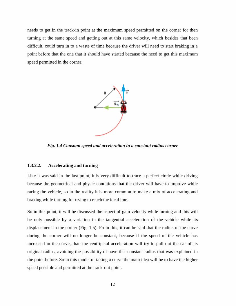
during the whole corner (Fig. 1.4).

Because in this case the same velocity is sustained in the whole corner, the driver will have

to do a hard effort for trying to start braking in the straight at the right moment because he

12

needs to get in the track-in point at the maximum speed permitted on the corner for then

turning at the same speed and getting out at this same velocity, which besides that been

difficult, could turn in to a waste of time because the driver will need to start braking in a

point before that the one that it should have started because the need to get this maximum

speed permitted in the corner.

Fig. 1.4 Constant speed and acceleration in a constant radius corner

1.3.2.2. Accelerating and turning

Like it was said in the last point, it is very difficult to trace a perfect circle while driving

because the geometrical and physic conditions that the driver will have to improve while

racing the vehicle, so in the reality it is more common to make a mix of accelerating and

braking while turning for trying to reach the ideal line.

So in this point, it will be discussed the aspect of gain velocity while turning and this will

be only possible by a variation in the tangential acceleration of the vehicle while its

displacement in the corner (Fig. 1.5). From this, it can be said that the radius of the curve

during the corner will no longer be constant, because if the speed of the vehicle has

increased in the curve, than the centripetal acceleration will try to pull out the car of its

original radius, avoiding the possibility of have that constant radius that was explained in

the point before. So in this model of taking a curve the main idea will be to have the higher

speed possible and permitted at the track-out point.

13

By trying to reach this model, it should be noticed that a lower velocity could be reached at

the track-in point for trying in the curve to accelerate the vehicle until its speed limit of the

curve. So it is really important to try to reduce the time in the curves of the whole race-

track because they usually represent a big part of the lap and are really fundamental for the

leaving a straight or for taking one.

Fig. 1.5 The acceleration of a particle5 in a curve:

a) The variation of the velocity and time components in a curve while accelerating.

b) The vectors of acceleration and velocity in a curve while accelerating.

1.3.2.3. Braking and turning

Due the importance of the corners in the laps it is precise to try to gain the major speed

possible in the track-in points as in the track-out points. So, like was explained in the point

before, for gaining the maximum speed possible in the track out point it is necessary that

the driver accelerate the car while it is in the corner. But, for getting the maximum speed

possible at the track-out point it could be used the ability of braking and turning in just a

part of the corner. So, what will happened when this model is executed is that the driver

will have the possibility of start braking in the straight in a point after the one that was

a) b)

14

supposed to be taken for entering into the corner at the higher speed possible, what will

permit to the vehicle to enter to the track-in point with a higher speed than the limit one in

the corner.

It is not logical to say that the vehicle will be braking and turning at the whole corner,

because if this happens then the speed of the car will be much less that the one expected, so

the brake and turning model will be applied in just a part of the corner which will be

usually after the track-in point.

In this case the vehicle will suffer the opposite consequence that the one that was described

in the last point, because instead of increase the velocity of the vehicle, the objective of this

model is to reduce the speed of the car. Like the velocity is slowing down, the tangential

acceleration is also slowing (Fig. 1.6) and so the variation in the curvature radius during

this section will be negative, what means that while the velocity is slowing down, the radius

will be getting shorter.

It is here when the driver should know how to mix the three models set up before, because

if the driver could handle this then the time in the lap will be optimum. So, the driver

should know basically when to start braking at the straights for entering at the track-in point

with a speed higher than the limit one (what will represent a gain in time in the straight

before the corner) for braking and turning in a section of the corner; after this he will have

to know the best point for start accelerating an turning in the remaining section of the

corner for reaching a velocity higher than the allowed in the corner at the track-out point

(what will represent a gain in velocity in the straight after the corner), minimizing in this

way the lap-times.

15

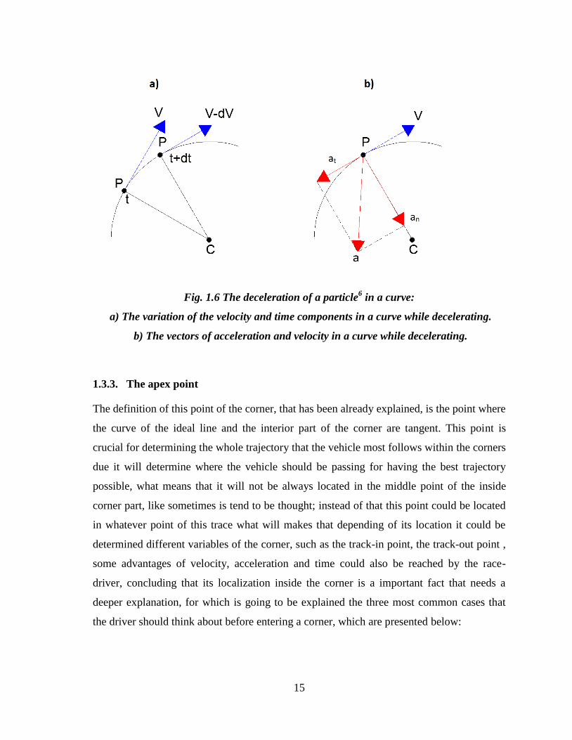
Fig. 1.6 The deceleration of a particle6 in a curve:

a) The variation of the velocity and time components in a curve while decelerating.

b) The vectors of acceleration and velocity in a curve while decelerating.

1.3.3. The apex point

The definition of this point of the corner, that has been already explained, is the point where

the curve of the ideal line and the interior part of the corner are tangent. This point is

crucial for determining the whole trajectory that the vehicle most follows within the corners

due it will determine where the vehicle should be passing for having the best trajectory

possible, what means that it will not be always located in the middle point of the inside

corner part, like sometimes is tend to be thought; instead of that this point could be located

in whatever point of this trace what will makes that depending of its location it could be

determined different variables of the corner, such as the track-in point, the track-out point ,

some advantages of velocity, acceleration and time could also be reached by the race-

driver, concluding that its localization inside the corner is a important fact that needs a

deeper explanation, for which is going to be explained the three most common cases that

the driver should think about before entering a corner, which are presented below:

16

The early apex-point.

The correct apex-point.

The late apex-point.

These three points are shown in the Figure 1.7, where could be noticed the regular behavior

that the vehicle has when it takes any of these trajectories that are actually conditioned by

where the apex point is located.

Fig. 1.7 The different apex points that could be taken

The first case, which is the one about the early apex-point that is represented in the Figure

1.7 with the red line, shows how the vehicle behaves in the corner, having an early turn-in

point, a bigger radius for taking the corner and a track-out point that due the bigger radius

would probably be out of the race-track, what is the same to say that because the radius that

the vehicle is following, the vehicle could be easier spitted out from the road. This type of

trajectory is usually taken, when the race-driver misses the properly track-in point, having a

major velocity than the one allowed for entering the corner, what will turn into a try for

reaching the correct apex-point while is following the trajectory but that it is immediately

17

traduced into an early apex-point and consequently, if the driver does not turn down the

speed of the vehicle then it will probably end out of the road. Analyzing the fact that the

vehicle has a major velocity in an early track-in point that the one that could have for a

regular track-in point, the disadvantage comes when it is begin to be talked about the track-

out point where for trying to conserve the gripe of the tires surges the of trying to reduce

the speed of the vehicle, having like a final result of the red line a speed that will be minor

that the one that the vehicle could have for a proper track-out point, and if this happens the

vehicle will start the next straight or corner with less speed than the expected, having like a

result a lost in the total lap-time.

Now, the correct apex-point is the one that is taken at the middle of the corner and which is

one of the points of the green trajectory that is shown in the Figure 1.7, which is the proper

line that could be chosen for that corner, where could be noticed that the biggest radius that

could fit in the curve had been taken, having like a result a normal turn-in point and a

correct track-out point, which means that the appropriates speeds had been taken for

entering and for leaving the corner.

Finally, the last kind of trajectories that could be taken in a corner is the one shown in the

Figure 1.7 with the yellow line, which corresponds to the late apex-point that is also

compound of a late track-in point and a late track-out point, having like a result a minor

radius that the one that was obtained when the “correct line” was taken, because is needed

to have a minor radius for having a trajectory that is still tangent to the inside part of the

corner (the late apex-point), having like an exit point a late track-out point, that like is

shown in the Figure is the safest track-out point that could be taken because is the one that

is farthest of the limits of the straight. But saying that is the safest condition, it does not

mean that is the best one that could be taken, because, having a smaller radius in a corner

will also means a minor speed for that corner, so probably the vehicle is in a safer

condition, but if the driver should have had abandoned the corner in the correct track-out

point, probably the speed of the vehicle would have been higher than the one that the

vehicle obtained leaving the corner in the late track-out point.

18

1.4. Annotations

1The ideal line in a corner.

2One of the wrong radius that could be taken.

3In the figure 1.3 the particle “P”.

4 This affirmation is equal for the straight parts of the track.

5The vehicle.

6The vehicle.

7http://www.nwalfaclub.com/track/images/apex.gif

19

CHAPTER 2. THE VEHICLE MODEL

In this chapter it will be introduced the different considerations that must be taken for

trying to reach the ideal line, because before this line is reached some boundaries would be

needed to be explained for trying to make the most realistic approach to the vehicle that is

trying to be descript. This approximation of the vehicle will be called the vehicle model,

and while the reader gets more involved in this subject, the idea of this model will open the

possibility to begin to understand the finality of this project, that like was said before, is to

try to develop a simulation showing the displacement of this vehicle model trough the ideal

line that is placed inside the race-track.

2.1. Model considerations

In this model is going to be descript all the factors that could intervene in the behavior of

the vehicle while it is been displaced by the road. For beginning, the car will be located in

an XY plane, which means that for the purpose of this investigation, the car will only be

allowed to move in a two dimensions plane. Saying this, is also important to know that the

car will have a reference point that will be located in the same plane in the point (0,0), so

the whole race-track will have a several quantity of point that could be plotted from this

reference point.

The model will be moving by a trajectory that will be compound by corners and straights,

but for a better approach, the whole model will be explained from the idea that this vehicle

is being displaced in a curve, because a straight is nothing more than a curve that has a

radius that is so big that it could be easily considered or approached like infinite, so it could

be thought that every segment of the race-track, even if is an straight, will be part of a

curve. Parting from this idea, the car will have a lot of variables involved in the

displacement of the vehicle in the race-track, between the ones exist the displacement,

speeds, accelerations, angular velocities, angular accelerations and a lot of angles that will

be changing while the model is moving. This concept is described in the Figure 2.1 where

20

all the variables that are involved in the displacement trough the race-track of the vehicle

are shown, fixed all of them in the gravity center of the car, which is the point where all of

these variables are applied.

Fig. 2.1 The vehicle model with all its parameters1

From the Figure 2.1, the first thing that should be noticed is the reference system, which is

a two dimensional system of coordinates represented by the plane XY with its positives

references shown in the Figure in the axes X and Y; the curvature radius of the mass center

of the vehicle model will be represented by the Greek letter ; the velocity of the vehicle

will be represented by the letter V and the angular velocity of the vehicle will be

represented by the Greek letter which represent the change of the angle in a corner in a

certain period of time. Because the curvature radius that the car will be describing, there

will be also involved a centripetal acceleration and a tangential acceleration represented by

n and t respectively; about this two vectors, it could be said that a sub-reference system

21

could be adopted, because the tangential acceleration will be always perpendicular to the

centripetal acceleration, which will permit to have two perpendicular axes, so this will be a

reference system that will be constantly changing by the movement of the vehicle and that

will be located between the axis “t” and the axis “n”.

In the Figure 2.1 it could also be noticed that there is a deviation of the car from its

tangential line, what will permit the possibility to a new sub-reference coordinated system

to exist, that will be located between the axes “x” and “y” and it is over this new sub-

system that the projections of the velocity will be located, that will represent the projections

of the velocity in every point of the road in this sub-system and that are represented by the

letters vx and vy respectively. About this new sub-reference system it could also be noticed

that it has a deviation angle between itself and the XY system, and this angle is represented

by the Greek letter , that like is shown in the Figure is also generated between the axis X

and the line that makes a transversal cut to the vehicle (x axis) and indicates the angle that

is generated between the direction line of the vehicle and the reference horizontal line of

the race-track.

There is another variable that is really important in the behavior of the vehicle and that will

determine how the behavior of the vehicle will be developed in the corner, and this one is

the angle between the tangential line of the mass center of the car (axis t) and the line that

marks the vehicle direction (axis x), this angle is represented by the Greek letter 2 and

will be determined by a new angular velocity, which will represent the rotation of the car

around its mass center and its represented by the letter . This angular velocity can be

different to the angular velocity ( ) of the center mass around the center of the circle,

because it will show how is the development of the tires of the vehicle in the curves, so the

more similar this angular velocities are, the better the traction the tires will have.

With the yaw angle are attached some new terms that will determine if the vehicle is

dripping off or if it is taking the corners properly, these new terms are “Oversteer” and

“Understeer”, which will be explained below.

22

2.1.1. Oversteer

Oversteer is a phenomenon that can occur in a vehicle while attempting to corner or while

already cornering. The car is said to oversteer (Fig. 2.2) when the rear wheels do not track

behind the front wheels but instead slide out toward the outside of the turn. The tendency

that a vehicle has for oversteering is affected by several factors such as mechanical

traction, aerodynamics and suspension and driver control, and should be applicable at any

level of lateral acceleration.

When cornering, oversteer describes more directional change than anticipated from a given

change of steering lock. The rear of the car steps out of line and the front of the car turns in

more than the anticipated. Limit oversteer occurs when the rear tires reach the limits of

their lateral traction during a cornering situation but the front tires have not, thus causing

the rear of the vehicle to head towards the outside of the corner.

Another way to describe this phenomenon is in terms of tire slip angle. Oversteer is also

said that occurs when the slip angle of the rear tires exceeds that at the front, which means

that the will be bigger than that in other words will be the same to say that the

angular velocity of the vehicle with respect to its center mass is bigger than the angular

velocity of the vehicle with respect to the center point of the corner that the vehicle is

taking, having like a result the phenomenon explained in this point, the Oversteer3.

23

Fig. 2.2 Images of a car oversteering.

2.1.2. Understeer

Understeer is the condition in which the vehicle does not follow the trajectory the driver is

trying to impose while taking the corner. Classically, understeer (Fig. 2.3.) happens when

the front tires have a reduction in traction during a cornering situation, thus causing the

front-end of the vehicle to have less mechanical grip and become unable to follow the

trajectory in the corner. When cornering, understeer describes the front of the car scrubbing

wide of the desired line, and thus the need to wind on more steering lock that would be

anticipated for a given directional change.

24

Fig. 2.3 Images of a car understeering.

Understeer occurs when the slip angle of the front tires exceeds that at the rear which

means that the will be lower than that in other words will be the same to say that the

angular velocity of the vehicle with respect to its center mass is lower than the angular

velocity of the vehicle with respect to the center point of the corner that the vehicle is

taking, having like a result the phenomenon explained in this point, the Understeer4.

2.1.3. A simplification of the model

As the goal of this project is to do an approximation of how the vehicle behaves in the real

life, some restrictions are going to be taken from the model that was explained before, for

trying to simplify the calculations and for having simpler Equations for the simulation

program that will be developed and explained in the next chapters. It is important to know

that these simplifications are not going to vary significantly the results from the reality, but

that there will be a certain percentage of error admitted for the finality of this project, and

25

that the approximation to the reality will have a certainty around 90%, which will be

enough for the end of this investigation.

If a deeper investigation will be required for getting a better percentage of certainty, like in

the real-world race line analyses, that requires a better approximation of the reality, the

considerations that are going to be taken in this point will not be valid and it will be needed

to have more elaborated programs, with more sub-routines that will throw more precisely

results.

So, the first consideration that it is going to be taken is that the velocity that was projected

in the axis “x” (vx) will be much bigger than the velocity projected in the axis “y” (vy),

making this vy velocity approximately equal to zero. This consideration will permit to

velocity projected vx to be the same to the total velocity of the vehicle V and with this

simplification the axis “x” will be transformed into the axis “t”, and the axis ”y” will

transform in to the axis “n”. This is the same to say that the yaw angle ( ) will be

approximately zero, so now the car will be oriented in the same line of the tangential line of

the mass center of the vehicle (Fig. 2.4.).

(Equation 2.1)

With this little simplification, it has also changed another variable that is important for

explaining the rotational behavior of the vehicle around the corner and around itself; since

the yaw angle it has transformed into approximately zero, the angular velocity of the mass

center of the vehicle around the center of the corner will be equal to the angular velocity of

the vehicle around its mass center, avoiding with this the variable of oversteering or

understeering the vehicle through the corner.

26

Fig. 2.4 Approximating the yaw angle to zero

The second consideration that will be taken for simplify the model will be to consider that

the curvature radius that the vehicle ( ) will have to follow in the road, will be much bigger

than the length between the front tires and the rear tires5 (Fig. 2.5), called “ ”.

(Equation 2.2)

27

Fig. 2.5 Comparison between the curvature radius that the vehicle follows and the length

between the front tires and the rear tires6

With this consideration the model is simplified in a lot of ways because, if this

consideration is not taken, than the velocity of each point of the car will be relatively

different than the one that the mass center has and so, each point of the vehicle will has its

own different inertia, making the calculations much more complicated. By doing this

simplification, the model vehicle will be reduced to a single particle (a point), that will

represent the movement of the vehicle trough the whole trajectory.

Now that the vehicle have been considered like a particle, all the variables that influence

the behavior of it, will be fixed to this single particle moving through the race-track, what

means that the behavior that this single particle will have while its being covered the

trajectory that should be taken will represent the real behavior of the vehicle in a simplified

model. So from this point, the model that will be considered will be the one that is shown in

the Figure 2.6, where the vehicle is properly represented like a particle.

28

Fig. 2.6 The model of the vehicle represented by a particle

It should be also considered, that like it is a model it will not represent perfectly the

behavior of the vehicle, but is good approximation of what the behavior of the vehicle

should be, having an error acceptable for the endings of the present investigation, so if it is

true that the results are not going to be the best that could be taken, certainly there will be

really nearby the results expected.

2.2. The friction circle

During the last points, it have been talked a lot about the variables that will be involved in

the behavior of the vehicle during the whole race-track, but since the objective of this

investigation is to try to determine the ideal line of the vehicle, this variables should be

known before determining this optimum trajectory that the vehicle should have to follow

for reaching the best time possible during the laps. But which of the variables are really

29

important for knowing how the behavior of the car will be during the laps? The answer for

this question, are the accelerations that the vehicle will experiment during the whole race-

track. But after this, comes a more controversial question which is, why the accelerations?

And this will be answered by saying that the accelerations are the change of the velocity of

the car in each point of the race-track, so this important variable that is divided in the

centripetal acceleration and the tangential acceleration will determine how the vehicle

behaves. This means that these both components of the acceleration will determine, into the

simulation system, how the vehicle (represented by a particle), takes every trace of the

track, and how it does change of speed and position while the time is running.

By knowing that the accelerations that the particle experiment in every point of the race-

track, it is vital to know how to determine this variables for every point, because this

variables will be changing by point to point. For knowing these accelerations, it will be

needed to have some geometrical limits (determined by the road) as well as acceleration

limits. For these last limits, it will be needed to use some theory for making the closer

approximation to the real-world vehicle behave, so it will be used a tool known as the

friction circle.

The components of the vehicle that are going to be responsible for transmit the change of

acceleration of the vehicle to the ground are the tires and these ones can only produce a

certain amount of traction (cornering force, grip, etc.), measured in “G-units” of

acceleration, which is a kind of measure that is used for determine the change of

acceleration of the vehicle. This measure is the rate between the acceleration that the

vehicle experiments and the total horizontal acceleration that the vehicle is experimenting

in every point of the lap. While the maximum force that a tire can take depends very much

on the current vertical load or weight on the tire, the acceleration of that tire does not

depend on the current weight. One "G" is equal to the amount of the acceleration gravity,

measured in a sideways instead of vertical direction. "Acceleration," in the engineering

sense, is defined as a change in "velocity." Velocity is composed of both speed and

direction. So acceleration means changing speed or changing direction, or both. This

acceleration applies not only when a vehicle is accelerating forward in the traditional sense,

but also applies when a vehicle is accelerating sideways (cornering at a steady speed), or

30

accelerating rearward (slowing down by braking). Assume that an hypothetical tire can

produce a maximum of only 1.0 G of acceleration, if the driver needs to speed up while

also covering a corner, the tires of the vehicle will still be limited to a total of 1.0 G. This is

shown in the Figure below (Fig. 2.7), which tries to explain the theoretical behavior of a

vehicle in whatever point of a race-track.

Fig. 2.7 The theoretical friction circle that a vehicle follows7

The axes that the diagram of the friction circle contempt, involves acceleration, braking,

left cornering and right cornering, resumed like a lateral acceleration vs. longitudinal

acceleration, which are indicated in the Figure 2.7 and that explains the combined variable

that a vehicle its experimenting in terms of acceleration, which is represented by G units of

acceleration. So, if a vehicle is cornering and accelerating, cornering and braking, just

accelerating or just braking, the vehicle will experiment a mixed behavior that will be

located between these axes and inside of the friction circle limits. This means that the point

of the acceleration could be located wherever inside this diagram, and it is here when the

limit of the friction circle begins to play a roll inside this diagram. It is important to notice

that the G units has no dimensions, so they are dimensionless, and this because it is a rate of

accelerations, so the units are cancelled and the best of all is that is not necessary to know

31

the weight of the car, so this law could be applied to whatever car, because it is just a

measure of the change in the rate of acceleration in every point in the time.

What this limit means, represented by a circle, is a limit of adherence that the tires could

have before sliding out of control in whatever point of the race-track. In the Figure 2.7, it

has been assumed a 1.0 G of acceleration for explanatory endings, and the acceleration that

a vehicle could have is generally measured using an electro-mechanical device called an

accelerometer. We all have a vertical acceleration of one G acting on us due the earth’s

gravity. Racing cars claim to be able to reach up to 3.5 G under acceleration and cornering,

and nearly 1.5 G under traction; this is because the engineering always tries to reach the

higher level possible of performance in its vehicles, so they are always submitted to the

highest conditions of design possible, permitting to the vehicle develop this higher

accelerations. On a more accessible level, a sports car on road tires is unlikely to reach one

G in cornering or under braking, though values of around 0.8 to 0.9 G are quite achievable.

Like it was said before, 1.0 G of acceleration will be used for explaining the diagram, so by

knowing this limit it could be said that if the vehicle has a combined acceleration minor

than 1.0 G of acceleration, than the vehicle will not slide out of the race-track and will have

the possibility to follow the path in the race-track at the highest speed permitted in each

point of the road. So, if the acceleration point of the vehicle is in the upper part of the

diagram (in the acceleration part) the vehicle will be winning speed, but if the acceleration

point of the vehicle is in the lower part of the diagram (in the braking part) the vehicle will

be losing speed. By saying this, it can be concluded that the best part where the acceleration

of the vehicle could be located is over the edge of the circle, which means that if this

happens the vehicle will be working at its limits of tire traction, and the curves and the

straights will be taken at the best way possible. In the real life, it is lot more complicated to

try to reach this acceleration limit without trespassing it, for which is needed a really

experimented driver and to know the real limit of the vehicle that its being driven, because

if this limit is trespassed than there will be a very big chance to the vehicle skid, making the

driver lose the control of the vehicle, even in a small proportion, what will be immediately

translated into a lost in lap-time in whatever point where the vehicle has skid out, because

32

the driver will try to recover the line that has been lost, compromising valuable time that

could make a huge difference in a race.

For a first approximation about the behavior of the variation of the acceleration of the

vehicle, this model of the friction circle diagram could be easily handled and sustained for

explaining the phenomenon that the vehicle experiments and how it should take every

single point of the road for avoid skidding out. But for making a closer appreciation of how

the vehicle behaves, there is a variation in the limits of this model represented by the same

axes, that receive the name of the “Modified Friction Circle” and that will be explained

below.

2.2.1. The modified friction circle

The modified friction circle is measured with the same parameters, is located inside the

same axes and it has like its origin point, the point (0, 0).

It is a derivation of the “Friction Circle” because it is a very similar limit representation,

that is also defined by the same circle but has a little variation in the traction part,

represented as a restriction that has a pattern of an arc of circle with a major radius that

closes the upper part of the friction circle limit (Fig. 2.8).

Assuming a car capable of support 0.9 G, as shown in Figure 2.8, the vehicle can turn left at

up to 0.9 G, brake at up to 0.9 G or turn right at up to 0.9 G, limited primarily by the grip

between the tires and the road surface. The suspension does have an effect in all of these

considerations, but it is main function here is to help the tires generate the grip that they are

potentially capable of.

33

Fig. 2.8 The modified friction circle8 &

9.

Under forward acceleration things are slightly different, as limiting factors other than tire

grip come into play. While in a low gear you may be able to spin the wheels, in higher

gears the available engine power becomes the limiting factor. This presents itself as a

distortion of the circle presented on the GG Diagram. The dashed line is what idealized

should happen, but the full line is what actually happens in a vehicle. Following this

diagram, it could be said that the safe ambient will be the range of points where the tires

reach their available grip. Outside this ambient, the vehicle will still be able to operate, but

not for very long because it will be operating under unstable conditions.

For understanding better this behavior there have been made some tests with

accelerometers for measure the real accelerations that a vehicle could experiment into a real

race-track. For this test it was used a Porsche 928S, which is a vehicle of high performance

and that was used for 8 minutes and its behavior was recorded by an accelerometer at 10

34

samples per second around the Sandown Motor Raceway to generate the trace shown.

These results are presented in the Figure 2.9, where clearly could be noticed that there is a

restriction in the acceleration part, so the upper limit is never trespassed and this due the

capacity that the motor of the vehicle has to accelerate.

Fig. 2.9 The GG Diagram of a Porsche 928S 10

Even in a high performance vehicle, this limit is not represented by the complete

circumference that was descript in the “Friction Circle Diagram”, what means that the

capability of the vehicle for accelerate will be restricted by the motor of every single

vehicle and each single vehicle will have a lower limit for accelerating than for braking,

concluding that the more the velocity the vehicle has reached, the most difficult is to try to

add more acceleration to the vehicle, which will be the same to say, that is more difficult to

add more speed to a vehicle if it is running at a high velocity because while the time is

passing, this vehicle is getting closer to its speed limit; the opposite happens if the vehicle

has a lower velocity because it is farther to its speed limit.

35

In the Figure 2.9 it must be highlighted that there is a big concentration of lines in the

vertical axis because a big part of the road must have been compound by straights. Also the

limit of acceleration was almost never reached and there is only one pike when the vehicle

almost reaches this superior limit. This because the limitation of the power of the motor

puts a restriction in the maximum acceleration that the vehicle could reach, so it is

confirmed the theory of the none constant radius arc in the traction part of the “modified

friction circle”, having for the same reason in the upper side of the Diagram a curve with a

larger radius that the one that the Friction Circle Diagram was supposed to have. Also it

should be noticed that this major radius circumference does not has it centers in the origin

and that the minor radius circumference is not a half of circumference, it is something about

¾ of circle due the mixed limit of turning and accelerating will be concentrated in this zone

and will be represented by the joining point of the major radius with the minor radius arc of

circle (Fig. 2.8).

Three particular points have been highlighted in the Figure 2.8. Point A is a small spike of

forward acceleration above what appears to be a fairly consistent horizontal boundary. The

recording of the acceleration data commenced before the car began moving. This spike

represents the acceleration of the car away from rest. Once moving, particularly around a

high speed circuit, the car has less acceleration capability. It is operating in a region where

it cannot attain as high a forward acceleration. This is the reason for the apparent boundary

of forward acceleration shown on the diagram.

Point B highlights that there is far more data displayed on the left side of the GG Diagram

than the right, so a car will spend much more time turning left than right. It is also apparent

that data occasionally appears beyond the curve defining the performance envelope. The

performance envelope indicates the sustained capabilities of a vehicle. Dynamic maneuvers

can exceed these capabilities, though only briefly, which is the reason why there are a few

picks of total acceleration, getting out and getting in (by a briefly period of time) of the

“modified friction circle” limits.

Point C indicates a spike arising from a dedicated maximum braking maneuver, executed

specifically to obtain an extreme value on the GG Diagram for later analysis. It is

interesting to contemplate whether this is a point arising from a dynamic maneuver, or a

36

sustained deceleration point, or some combination of both. The point itself peaked at a

deceleration value of 1.25 G, which is quite an impressive Figure for a road car.

37

2.3. Annotations

1 Class notes: Mauro Speranza Neto, 2009.

2 Also known as the yaw angle, which is a phenomenon that is developed whenever the

vehicle changes of direction, having like a result an angle between the direction of travel

and the centerline of the racecar.

3http://www.mgf.ultimatemg.com/group2/suspension/tracking.htm.

4http://www.mgf.ultimatemg.com/group2/suspension/tracking.htm.

5 The wheel base.

6 Class notes: Mauro Speranza Neto, 2009.

7 Lee, Johns. The friction circle: The secret of vehicle control.

8 The modified friction circle is plotted within the GG Diagram.

9 McIver, John. The GG Diagram. 1996.

10 McIver, John. The GG Diagram. 1996.

39

CHAPTER 3. CONSTRUCTING THE IDEAL LINE

For trying to make a better explanation of how the lap-time of the vehicle is modified

depending of the trajectory that is has been chosen by the race driver, it has been developed

different possible solutions that will involve different procedures that at the end will lead to

the best path to follow, being this the ideal line for this problem.

The limitations that have been considered for the problem are physical and geometrical; the

physical are the ones that involve the limitations of the behavior of the vehicle, between the

ones could be mentioned the velocity limits and the acceleration (accelerating and braking)

limits of the vehicle. The geometrical are the one referred about the race track, what means

that the different paths that could probably be taken are going to be located inside the race-

track, and that this limit could not be trespassed by the vehicle, otherwise it would be

running out of the race-track, conditioning the vehicle to try to reach the ideal line between

this parameters.

Different programs have been used for building the race-track and for calculating the lap-

times of the different paths that could be taken by the race driver; between this programs,

for designing the race-track it has been used Autocad, which is a tool that handles the

design of whatever that is needed to be built, that in this case was the race-track; by the

other hand for making an initial calculation of the lap-times it has been made an interaction

between the programs Autocad and Microsoft Excel, because is needed a link of measure-

calculating which is reached with the combinations of these two programs; with Autocad it

has been used the measure tool, for then inserting this measures in the Microsoft Excel

Worksheets, which is the tool in charge of calculate, by different formulas given to the

Excel program, the lap-time that each trace followed by the vehicle represents.

There were a lot of possibilities of race-tracks to be chosen for developing the

investigation, but in order to be perfecting the concept of the ideal line in a simplified

model it has been chosen one race track with 6 corners of 90° degrees accompanied by 6

straights traces. That race-track is shown in the Figure below (Fig. 3.1.) with its

corresponding dimensions.

40

Fig. 3.1 The race-track chosen for develop the ideal line1

This race-track was chosen due it is easy for being evaluated and because if the proper ideal

line is reached then there will not be a need to evaluate different paths to be taken in a more

complicated race-track, going directly to establish the path that gives a better lap-time for a

vehicle and simulating it in the Matlab program that will shows the vehicle moving through

this race-track.

At below, there will be shown and explained the different paths that a race driver could

take, showing there, the real path designed in Autocad, the formulas used for calculating

the time that the vehicle spend in the lap and different considerations that were assumed for

each model.

41

3.1. Path # 1: Through the center of the race-track at a constant speed

Since the principal objective of this investigation is to try to find the ideal line that a vehicle

could have in the race-track previously shown, there will be evaluated different paths that

could probably be taken for comparing the lap-times in each path. The first and simpler

trajectory that the vehicle could follow is at the middle of the road in every point of the

race-track at a constant speed.

By saying that, the vehicle will have a constant speed at the whole track, so some

considerations most be taken for developing this kind of theoretical behavior. First of all,

for comparison endings it would be considered that since the “zero point”2 the vehicle will

have a determined speed that will be different for each case. In this special case, a constant

speed will be handled by the vehicle in the whole race-track, which is the reason why the

vehicle was not began to be evaluated since the rest, because if it does start from this

condition, a change in the acceleration will be needed to be applied, but like in this first

case, the simpler case was tried to be explained, then is not going to be considered this

change of acceleration in the vehicle. As well there should be used the maximum speed

allowed by the road, that will be fixed by the geometrical place where the minimum

velocity could be reached, that is the corner with the minimum radius due the centripetal

acceleration in the curves will be always the same and so the maximum speed in the corner

with the minor radius will determine the speed that will be fixed in the whole race-track;

like in this case all the radius of the race-track are equals, then is from this constant radius

where the maximum speed for the whole race-track will be obtained.

The path for this case, with all its measures and with its starting point it is shown in the

Figure below (Fig. 3.2.)

42

Fig. 3.2 The path of the vehicle by the center of the road

Like it was explained in the chapter 2, in the point of the friction circle, the same limit of

accelerations will be used for each of the paths that will be developed, but the limits of

accelerations will be different that the ones explained in that point; these are shown in the

Table 3.1.

Acceleration limits

Centripetal (G) Tangential (G)

Turning left Turning right Accelerating Braking

-4 4 1.5 -4

Table 3.1 The acceleration limits

43

The acceleration limits shown in the past Table has values that a regular vehicle will

probably not resist in normal conditions, but due it is been evaluated a high performance

vehicle which is capable to support this big changes of velocity, then these conditions could

be applied to the vehicle in the whole race-track. Now, the graphic showing the acceleration

limits that a vehicle could have during the whole race-track are shown in the Figure 3.3 like

a modified friction circle limits, but with the values of the Table 3.1.

Fig. 3.3 Modified friction circle limits for a high performance vehicle

Like it has been explained before, in this special case a constant speed will be assumed

through the whole race-track what will lead to a constant centripetal acceleration in the

corners as well as a tangential acceleration of zero through the whole trajectory. Due the

acceleration will be constant in the corners, it could be used the Equation 1.4. for determine

the maximum velocity that the vehicle could has, before reaching its centripetal

acceleration limit that for these case will have a value of 4.0 G for the whole corner. So it

was evaluated in a Microsoft Excel Worksheet, making variations of 0.5 km/h in the

velocity since 0 until 300 km/h and it was determined that the maximum velocity that the

vehicle could handle in this curve with a radius of R=56.25 m, was of V=170.5 km/h (47.36

-5

-4

-3

-2

-1

0

1

2

-6 -4 -2 0 2 4 6

Centripetal acceleration

Tangential acceleration

The modified friction circle limits

44

m/s). So the vehicle will have this velocity through the whole path which has a total length

of 2150.14 m.

Now, for the calculation of the lap-time of the vehicle in this case it will be used an

Equation for a constant velocity, which it is shown below.

(Equation 3.1)

In the Equation 3.1, “t” is the time that the vehicle will need for complete the lap, “ΔS” is

the portion of race-track that will be followed at a “V” constant velocity that for this case

will be the complete trajectory at the middle of the road. At making the calculations in the

Microsoft Excel Worksheet, the result obtained from using the Equation 3.1 in the actual

race-track will lead to a total lap-time of 45.40 s. This result of time will be next used for

making a comparison between the different lap-times of the paths taken and for perfecting

the optimum trajectory to be chosen for showing that this first path taken will be far away

from the optimum time that could be reached if the vehicle has had chosen the ideal line

and variations of velocity and acceleration through the road.

3.2. Path # 2: Taking the maximum radius in the corners, considering

changes of acceleration and velocities trough the time

This second possibility of path that could be taken will be fixed by three crucial parameters

that will set the trend of behavior of the vehicle through the race-track, which are:

Take the maximum radius of the race-track: That was made with the help of one of

the tools of Autocad, which gives you the opportunity to trace an arc of

circumference by making tangential points in three different parts of the race-track

(Fig. 3.4), which are:

A point in a parallel line of the straight with an offset of 1 m 3 of the line that is

farthest from the center of the coming corner4.

A point in a 1 m offset circle of the inside circumference of the corner5.

45

A point in a parallel line of the straight with an offset of 1 m of the line that is

farthest from the center of the past corner6.

Consider that the velocity will be changing in every single point of the race-track, so

the acceleration will be also changing in every point. By having this consideration,

there will be needed to set a parameter of change of the acceleration, this parameter

will be after explained.

In the zero point (which will be tried to be located in the same position or at least in

the same sector for all the trajectories), the vehicle will have an initial velocity of

zero, this in order to try to compare this case with the other ones.

Fig. 3.4 The three points for making the maximum radius in a corner7

In the particular case of the race-track that is actually being evaluated, it is compound by 6

equal corners, what means that the maximum radius for one corner will be the same

maximum radius for the other corners, having the same behavior of velocities and

accelerations in all the corner of this race-track.

For set the acceleration behavior that the vehicle was going to follow in the race-track, it

was used the parameter set by Carl Lopez in one of his racing books8, where he tries to

46

explain the regular behavior that a vehicle should follow, which is an approximation about

what really happens in the real life, having this behavior like a parameter for the rest of the

investigation. The acceleration behavior of the vehicle in whatever race-track is shown in

the figure below (Fig. 3.5)

Fig. 3.5 The acceleration behavior of the vehicle in the race-track

The acceleration behavior that is shown in the Figure 3.5 could be used for whatever race-

track, because they will be compound by straights that are always located before the curves.

This behavior could be resumed by the next explanation: Being in the straight that is before

the corner by accelerating the vehicle (traction) or at a constant velocity (depending of its

length), for then beginning to brake for entering the corner; when the corner is reached,

keep braking by a ¼ piece of the corner, for then start accelerating the vehicle (traction)

until the exit of the corner has been reached (the resting ¾ piece of the corner); after the

track-out point has been reached, depending on the condition of the following straight (its

length), there will be needed to follow accelerating or to keep the vehicle with a constant

velocity before entering the next corner.

47

The path to be followed by the vehicle in this case was designed one more time with the

Autocad program, because it is a tool that makes easier the design of the trajectory to be

followed. The trajectory, its dimensions and the localization of the zero point are shown in

the Figure 3.6.

Fig. 3.6 The path of the vehicle by the maximum radius

For the analysis of this case, the race-track will be divided in twelve traces that will be

separately studied for determine the time needed to cover each trace of the path, due each

trace that the vehicle cover will have its own behavior and for future studies, if the same

analysis is needed to be executed, the race-track is going to be divided in how many traces

48

how necessary. The traces in which this specific race-track was divided are shown in the

Figure 3.7 with its proper enumeration.

Fig. 3.7 The different traces in which the race-track was divided

3.2.1. Explaining the traces

3.2.1.1. The curves

It could be noticed and it was explained before, that for this race-track there will be some

traces that will have the same dimensions, so for this case is there where the analysis

begins. These traces that are equals are the quarters of circumference that are inserted in the

six corners that the race-track contains for achieve the maximum radius there, which are the

traces 2, 4, 6, 8, 10 and 12. These maximum radius of these corners have a value of

R=94.13m and are 90° corners, which for this analysis will be divided in 16 little traces

which will be distributed between a braking zone and a accelerating zone. The braking zone

will possess the quarter of the circumference arc (22.5° of the 90° corner) and the

accelerating zone will possess three quarters of the circumference arc (68.5° of the 90°

corner)9; The 4 first mini-traces will correspond to the braking zone and the 12 remaining

mini-traces will correspond to the accelerating zone.

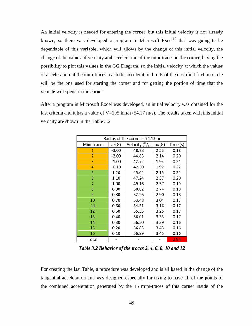
49

An initial velocity is needed for entering the corner, but this initial velocity is not already

known, so there was developed a program in Microsoft Excel10

that was going to be

dependable of this variable, which will allows by the change of this initial velocity, the

change of the values of velocity and acceleration of the mini-traces in the corner, having the

possibility to plot this values in the GG Diagram, so the initial velocity at which the values

of acceleration of the mini-traces reach the acceleration limits of the modified friction circle

will be the one used for starting the corner and for getting the portion of time that the

vehicle will spend in the corner.

After a program in Microsoft Excel was developed, an initial velocity was obtained for the

last criteria and it has a value of V=195 km/h (54.17 m/s). The results taken with this initial

velocity are shown in the Table 3.2.

Table 3.2 Behavior of the traces 2, 4, 6, 8, 10 and 12

For creating the last Table, a procedure was developed and is all based in the change of the

tangential acceleration and was designed especially for trying to have all of the points of

the combined acceleration generated by the 16 mini-traces of this corner inside of the

Radius of the corner = 94.13 m Mini-trace at (G) Velocity (m/s) an (G) Time (s)

1 -3.00 48.78 2.53 0.18 2 -2.00 44.83 2.14 0.20 3 -1.00 42.72 1.94 0.21 4 -0.10 42.50 1.92 0.22 5 1.20 45.04 2.15 0.21 6 1.10 47.24 2.37 0.20 7 1.00 49.16 2.57 0.19 8 0.90 50.82 2.74 0.18 9 0.80 52.26 2.90 0.18

10 0.70 53.48 3.04 0.17 11 0.60 54.51 3.16 0.17 12 0.50 55.35 3.25 0.17 13 0.40 56.01 3.33 0.17 14 0.30 56.50 3.39 0.16 15 0.20 56.83 3.43 0.16 16 0.10 56.99 3.45 0.16

Total - - - 2.94

50

modified friction circle limits. So it could be said that this change of tangential

accelerations was reached by proof and error, getting like a result, the points of the second

column of the Table. These tangential accelerations were applied from the initial point until

the exit point of each mini-trace11

.

For the third column, that is the column of velocities for each mini-trace, the next formula

was used.

(Equation 3.2)

Where, “Vf” is the final velocity of each mini-trace; “V0” is initial velocity for each mini-

trace; “at” is the tangential acceleration applied to each mini trace, needed for the change of

velocities; “ΔS”, is the length of the mini-trace, that in this case it is a 1/16 portion of the

quarter of the arc of circumference and that will have for this corner a value of ΔS=9.24 m.

So for the column of velocities the first value of initial velocity is needed for have a starting

point and for calculating the final velocity of the first mini-trace, then the initial velocity of

the second mini-trace will be the final velocity of the first mini-trace for then being able to

calculate the final velocity of the second mini-trace and so on for calculating the velocities

of the resting mini-traces. So it could be concluded that the velocity calculated and

registered for each mini-trace is actually the final velocity of each mini-trace.

Now, the third column was calculated with the Equation 1.4, where the centripetal

acceleration is equal to the square of the velocity in each point of the corner, divided by the

radius of the corner (that for this is case was considered like continuous). This last value

will represent the centripetal acceleration in “m

/s2” units, but due for plot the centripetal

acceleration in the GG diagram it is needed to have the units of the tangential and

centripetal acceleration dimensionless (actually in “G Units”), the value obtained from the

Equation 1.4 its divided by the G acceleration, which is the gravity acceleration and that for

this case will have a value of 10 m

/s2, that are the real values that appear in the 3

th column.

51

Finally, after it has been obtained the correct acceleration points (tangential as well as

centripetal), it was calculated the time that the vehicle spend in each mini-trace and it was

tabulated in the 3th

column. The final result of the time that the vehicle spent in the corner is

shown at the end of the 3th

column inside a red box and is the sum of the time spent in each

mini-trace.

It is also important to mention that this final time that is located in the red box of the Table,

is the final time just for one corner and that at the end of the explanation of the other traces,

there will be examined the develop of the velocity and acceleration of the vehicle through

the whole time that it has spent in the lap by some graphics that will explain easier this

behavior.

For the considerations of velocity that were obtained in the Table 3.2, the graphic in the

Figure 3.8 was obtained and it could be noticed that all of the points plotted are inside of

the modified friction circle limits. It should also be noticed that in the Figure 3.8 are plotted

two graphics, and this graphic that have like difference the sign of the centripetal

acceleration and this is because the graphic that is located at the right side of the origin

represents the curves that was taken to the right, and the graphic that is located at the left

side of the origin represents the curves that was taken to the left side. In the race-track that

is being evaluated exist 5 corners taken to the right side and one corner taken to the left side

(Figure 3.6).

52

Fig. 3.8 The GG Diagram for the biggest radius corners

3.2.1.2. The straights

Now that the corners has been explained, it would be explained the behavior of the vehicle

in the straights that will depend of its location inside the race-track, what means that if a

straight is located between two corners that will be taken for the same side (the both to the

left or the both to the right) than the straight will be taken like an straight; but if instead the

straight is located between two corners that are going to be taken for different sides (one to

the left and one two the right12

) than the straight will be taken in a kind of curve called “S

curve” because it will be needed to pass from one side of the straight to the other one, so

this kind of curve is taken in a straight for making the change of side of corner the

smoothest as possible.

So first will be explained the straights that are going to be taken like straights. For these

ones the behavior will be the next one:

-5.00

-4.00

-3.00

-2.00

-1.00

0.00

1.00

2.00

-6.00 -4.00 -2.00 0.00 2.00 4.00 6.00

an

at

GG Diagram for the corners

53

The part of the straight where the vehicle is accelerating is named the traction part,

and in this part it was used the behavior of the graphic shown in the Figure 3.9,

where depending from the velocity in whatever point of the traction part of the

straight there will be a corresponding acceleration according with the graphic. So

for example if the vehicle is experimenting a velocity of 25 km/h, then the

acceleration between 25 and 50 km/h will have a value of 1.5 G and so on for all of

the values of the velocity within the speed limits of the vehicle that are between 0

and 300 km/h

Fig. 3.9 “a vs. V” in traction in a straight

The part for decelerating the vehicle without trespassing its acceleration braking

limit, that in this case will be used a limit lower than the maximum, having for this

part an acceleration of 3 G. This deceleration will be applied until the vehicle reach

the speed needed to enter the curve. It was not used the braking limit due, this

deceleration was considered that was going to be applied to the whole braking part

of the straights, so for getting the closer as possible to the real behavior of the

vehicle, it was decided to use the acceleration before indicated.

0.00

0.20

0.40

0.60

0.80

1.00

1.20

1.40

1.60

0.00 50.00 100.00 150.00 200.00 250.00 300.00

a (G

)

V (km/h)

"a vs. V" in traction in a straigth

54

There will also exist a part where the vehicle will have a constant velocity. This part

will be located after the vehicle has reached its speed limit and before the vehicle

starts braking.

The first straight that will be explained is the trace 1 which has a length of 495.98 m and

that was tabulated with all its values of velocity, acceleration, distances and times in the

Table 3.313

.

Trace # 1

Mini-trace at (G) Distance (m) Velocity (m/s) Time (s)

1 1.50 6.43 13.89 0.93 2 1.25 23.15 27.78 1.11 3 1.00 48.23 41.67 1.39 4 0.75 90.02 55.56 1.85 5 0.50 173.61 69.44 2.78 6 0.25 104.54 73.11 1.47 7 0.00 0.14 73.11 0.00 8 0.00 0.14 73.11 0.00 9 0.00 0.14 73.11 0.00

10 0.00 0.14 73.11 0.00

11 -3.00 8.24 69.65 0.12 12 -3.00 8.24 66.01 0.12 13 -3.00 8.24 62.15 0.13 14 -3.00 8.24 58.04 0.14 15 -3.00 8.24 53.61 0.15

16 -3.00 8.24 48.78 0.16

Total - 495.98 - 10.34

Table 3.3 Behavior of the trace 1

The point where the past Table was began to be evaluated is the final velocity of the

braking part due it is the same velocity for starting the following corner so it will fix the

appropriate velocity at what the vehicle should abandon the straight and it was obtained

from the Table 3.2. Then the initial velocity of the braking part was assumed and is the one

which it could be played and is called the “equilibrium velocity” and is the one that

determines if a constant velocity part will exist, considering that the initial velocity of the

braking part will be equal to the final velocity of the accelerating part. For this straight the

55

equilibrium velocity had a value of 73.11 m

/s (263.2 km

/h). Now the initial velocity of the

accelerating part will be determined by the exit velocity of the last corner that is already

known and it was also taken from the Table 3.2.

The distances represented from the change of velocities of the accelerating part and of the

braking part were obtained from a variation of the Equation 3.2 which is shown below.

(Equation 3.3)

So if the sum of the distance of the accelerating part with the braking part is major than the

total length of the straight then it should be changed the equilibrium velocity (that like was

explained before, it could be easily changed in the program generated in Microsoft Excel).

Now if the sum of the distances of the accelerating part with the braking part is minor than

the length of the straight then there will also exist a constant velocity part which will be

given by the next Equation.

(Equation 3.4)

Being “ ” the length covered at a constant velocity, “ ” the total length of the

straight, “ ” the length covered when the vehicle is accelerating and “ ” the

length covered when the vehicle is decelerating for entering the next corner. So the

intention of the program will be to try to reduce the length covered at a constant velocity

the most as possible for trying to have the bigger traction length possible.

For calculating the times that the vehicle spends in each part of the straight there will be

used two different Equations, one used for the parts where the velocity is changing through

the time and the other one for the part where the velocity is constant; these Equations are

shown below.

(Parts with acceleration) (Equation 3.5)

56

(Part with constant velocity) (Equation 3.6)

After each time has been calculated, it could be summed for obtain the total time that the

vehicle has spent in the trace # 1, which is the sum of the time that the vehicle spent in the

accelerating part, the constant part and the braking part, having like a result a time of 10.34

seconds for this straight, that was shown in the red box of the Table 3.3.

The other traces into the race-track that will have a similar behavior that the one that the

vehicle has in the trace # 1 are going to be the traces # 3, 9 and 11, which corresponding

Tables are going to be shown below.

The results of the behavior of the trace # 3 were tabulated in the Table 3.4, where the

variables were applied to the vehicle in a total length of 83.48 m, with the same conditions

of the Table 3.3, knowing that the acceleration that will be applied for each mini-trace in

the traction part will depend of the graphic shown in the Figure 3.9.

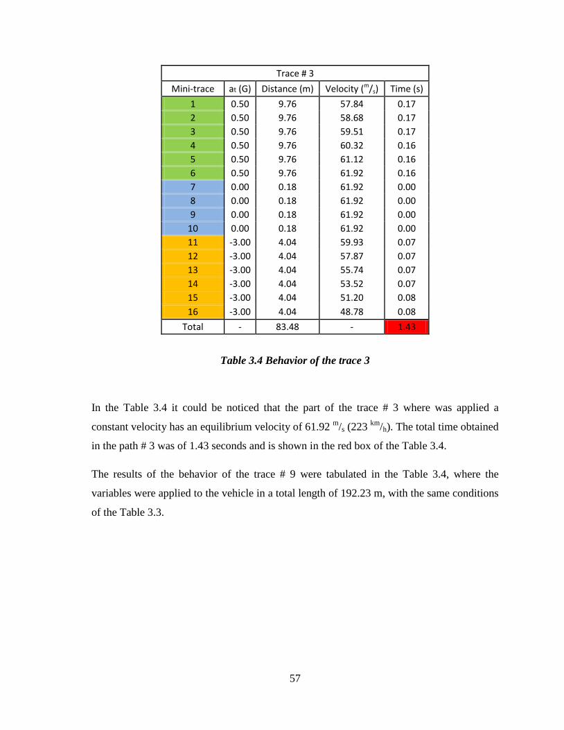
57

Trace # 3

Mini-trace at (G) Distance (m) Velocity (m/s) Time (s)

1 0.50 9.76 57.84 0.17 2 0.50 9.76 58.68 0.17 3 0.50 9.76 59.51 0.17 4 0.50 9.76 60.32 0.16 5 0.50 9.76 61.12 0.16 6 0.50 9.76 61.92 0.16 7 0.00 0.18 61.92 0.00 8 0.00 0.18 61.92 0.00 9 0.00 0.18 61.92 0.00

10 0.00 0.18 61.92 0.00 11 -3.00 4.04 59.93 0.07 12 -3.00 4.04 57.87 0.07 13 -3.00 4.04 55.74 0.07 14 -3.00 4.04 53.52 0.07 15 -3.00 4.04 51.20 0.08

16 -3.00 4.04 48.78 0.08

Total - 83.48 - 1.43

Table 3.4 Behavior of the trace 3

In the Table 3.4 it could be noticed that the part of the trace # 3 where was applied a

constant velocity has an equilibrium velocity of 61.92 m

/s (223 km

/h). The total time obtained

in the path # 3 was of 1.43 seconds and is shown in the red box of the Table 3.4.

The results of the behavior of the trace # 9 were tabulated in the Table 3.4, where the

variables were applied to the vehicle in a total length of 192.23 m, with the same conditions

of the Table 3.3.

58

Trace # 9

Mini-trace at (G) Distance (m) Velocity (m/s) Time (s)

1 0.50 25.34 59.17 0.44 2 0.50 25.34 61.28 0.42 3 0.50 25.34 63.31 0.41 4 0.50 25.34 65.28 0.39 5 0.50 25.34 67.20 0.38 6 0.50 25.34 69.06 0.37 7 0.00 0.09 69.06 0.00 8 0.00 0.09 69.06 0.00 9 0.00 0.09 69.06 0.00

10 0.00 0.09 69.06 0.00 11 -3.00 6.64 66.11 0.10 12 -3.00 6.64 63.03 0.10 13 -3.00 6.64 59.78 0.11 14 -3.00 6.64 56.36 0.11 15 -3.00 6.64 52.70 0.12

16 -3.00 6.64 48.78 0.13

Total - 192.23 - 3.09

Table 3.5 Behavior of the trace 9

A similar result was obtained and tabulated with the trace # 9, where with a speed of 69.06

m/s (248.6

km/h) the constant velocity part was covered. The total time that the vehicle spent

in this trace was of 3.09 seconds and is shown in the red box of the Table 3.5.

Finally, given the conditions of the race-track, the last straight that was actually taken like a

straight is the trace # 11, which length was of 300.98 m. The results of the variables applied

in this trace are shown in the Table 3.6.

59

Trace # 11

Mini-trace at (G) Distance (m) Velocity (m/s) Time (s)

1 0.50 52.48 61.42 0.89 2 0.50 52.48 65.56 0.83 3 0.50 52.48 69.44 0.78 4 0.25 31.60 70.57 0.45 5 0.25 31.60 71.68 0.44 6 0.25 31.60 72.78 0.88 7 0.00 0.03 72.78 0.00 8 0.00 0.03 72.78 0.00 9 0.00 0.03 72.78 0.00

10 0.00 0.03 72.78 0.00 11 -3.00 8.10 69.36 0.11 12 -3.00 8.10 65.76 0.12 13 -3.00 8.10 61.95 0.13 14 -3.00 8.10 57.90 0.14 15 -3.00 8.10 53.53 0.15

16 -3.00 8.10 48.78 0.16

Total - 300.98 - 5.07

Table 3.6 Behavior of the trace 11

In this trace the maximum velocity reached in the straight (the equilibrium velocity) has a

value of 72.78 m

/s. Now, the time spent in this trace reached a value of 5.07 seconds which

is shown in the red box of the Table 3.6.

There are still missing two straights that were not assumed like the rest of straights because

there are located between two corners that are need to be taken for different sides (one to

the left side and the other one to the right side), so like was explained before, these kind of

straight is not taken like they were straights, instead of that a “S curve” is used for cover

this kind of straight due the change of side should be made the smoothest as possible,

having the necessity of make this kind of curve inside of these straights for the well of the

lap-time. So for this race-track, these “S curves” will be applied in the resting traces that

have not been explained yet, which are the traces # 5 and # 7 that like shown in the Figure

3.6 will have this kind of behavior. What taking these straights like “S curves” mean is that

two equal constant radius arc of circle were joined at the middle of the straight for trying to

60

use the same kind of the methodology used in the corners with the only difference that the

angle covered by the vehicle in these cases is different. At the end, for making easier the

calculations these “S Curves” of each straight were considered like a single arc of

circumference that has an equivalent angle of the sum of the two joined arcs of circle angles

of the S Curve, what is the same to say that is twice of the angle of one of the arc of

circumferences of the S Curve.

The Tables that were created for explaining the behavior of the vehicle have their own

pattern due the mini-traces created for cover the “S Curves” were constantly changed until

a satisfactory result was obtain. Below in the Table 3.7 it is shown the behavior of the

vehicle in the trace # 5.

Table 3.7 Behavior of the trace 5

It could be noticed that there were used the same number of mini-traces for evaluating the S

Curve than for evaluating the corners, which means that the complete angle of the S Curve

was divided by the 16 mini-traces, that for the special case of the trace # 5 has an arc of

circle of 22 degrees, with a constant arc radius of 338.22 m. The difference that exists

between the Tables is that for this one the first part of the trace (12 first mini-traces) was

Radius of the corner = 338.22 m Mini-trace at (G) Velocity (m/S) an (G) Time (s)

1 1.10 58.54 1.01 0.14 2 1.06 59.99 1.06 0.14 3 1.02 61.36 1.11 0.13 4 0.98 62.64 1.16 0.13 5 0.94 63.84 1.21 0.13 6 0.90 64.98 1.25 0.13 7 0.86 66.04 1.29 0.12 8 0.82 67.04 1.33 0.12 9 0.78 67.98 1.37 0.12

10 0.74 68.86 1.40 0.12 11 0.70 69.68 1.44 0.12 12 0.66 70.44 1.47 0.12 13 -1.50 68.69 1.40 0.12 14 -1.00 67.50 1.35 0.12 15 -0.50 66.90 1.32 0.12 16 -0.50 66.29 1.30 0.12

Total - - - 1.99

61

used for accelerating and the final part of the trace (the 4 resting mini-traces) was used for

braking the car before entering the corner14

, which is an inverse behavior that the one used

in the Table 3.2. About the variables of the Table 3.7 against the variables of the Table 3.2.,

there were practically obtained with the same Equations, so the explanation about how

there were obtained is not needed because it was already done for the Table 3.2, having the

behavior of the acceleration plotted in the GG Diagram in the Figure 3.10.

Fig. 3.10 GG Diagram for the trace 5

The value of time that was spent in the “S Curve” of the trace # 5, is indicated in the red

box of the Table with a value of 1.99 seconds.

The trace # 7 is the last straight taken like an “S Curve” which has a different length than

the trace # 5, so respectively a different radius of “S Curve” will need to be taken, which in

this case will be a minor radius with a value of 107.37 m. A different angle is also used for

this S Curve, with a value of 32 degrees. Now that has been explained, the behavior of the

trace # 7 is shown in the Table 3.8, which is below.

-5.00

-4.00

-3.00

-2.00

-1.00

0.00

1.00

2.00

-6.00 -4.00 -2.00 0.00 2.00 4.00 6.00

an

at

GG Diagram for the S Curves

62

Radius of the corner = 107.37 m

Mini-trace at (G) Velocity (m/S) an (G) Time (s)

1 1.10 57.71 -3.10 0.07 2 1.06 58.40 -3.18 0.06 3 1.02 59.05 -3.25 0.06 4 0.98 59.67 -3.32 0.06 5 0.94 60.25 -3.38 0.06 6 0.90 60.81 -3.44 0.06 7 0.86 61.34 -3.50 0.06 8 0.82 61.84 -3.56 0.06 9 0.78 62.31 3.62 0.06

10 0.74 62.75 3.67 0.06 11 0.70 63.17 3.72 0.06 12 0.66 63.56 3.76 0.06 13 -1.50 62.67 3.66 0.06 14 -1.00 62.07 3.59 0.06 15 -0.50 61.77 3.55 0.06

16 -0.50 61.46 3.52 0.06

Total - - - 0.98

Table 3.8 Behavior of the trace 7

Like for the Table 3.7, the Equations needed for obtain all of the variables of the Table 3.8,

was before explained for obtaining the variables of the Table 3.2., which like a final result

has the total time of the “S Curve”, that is indicated in the red box of the Table 3.8 and that

has a value of 1.1494 seconds.

The behavior of the accelerations of the vehicle in the S Curve of the trace # 7 was plotted

in the Figure 3.11, which is shown below.

63

Fig. 3.11 GG Diagram for the trace 7

Now that all the traces have been explained is important to describe the tendency that the

vehicle experiments while is covering the whole trajectory, due this is going to be plotted

the behavior of the different variables that affect directly the vehicle against the time while

these variables are applied to the vehicle through a complete lap, considering for this case

that the maximum radius was taken in all the corners, but that the maximum accelerations

permitted for this vehicle was not used due the limitation of the radius, having all of the

accelerations inside the modified friction circle limits (Fig. 3.8).

The first graphic that is going to be explained is the one of the velocity of the vehicle in

every point of the trajectory vs. the time that the vehicle spends in the lap, which is shown

in the Figure 3.12, where it could be noticed that the vehicle suffers rises of velocity for

reaching a pick point in every concavity (that will be determined by the limits of speed of

the vehicle or by the geometric limits of the race-tracks) for then slowing the vehicle and

having a minimum velocity that for this case is going to be the same for every change of

curve15

of the graphic due it was considered that the six corners of this race-track was going

to have the same radius, so a same behavior will be obtained for the corners having like a

result a same minimum velocity for each corner. All of the points plotted in this graphic are

-5.00

-4.00

-3.00

-2.00

-1.00

0.00

1.00

2.00

-6.00 -4.00 -2.00 0.00 2.00 4.00 6.00

an

at

GG Diagram for the S Curves

64

positive due the magnitude of the vehicle will be always positive having only changes of

the direction and magnitude of this vector through the time.

Fig. 3.12 Velocity of the vehicle vs. time in one lap

It should also be noticed that the pick points of the curves are different between each

others, because there are some straights where the speed limit of the vehicle was not

reached due the length of the straights16

.

The tendency in all of the rises of velocity has a kind of logarithmic trend with a speed

limit, due while the vehicle is winning velocity is more difficult for itself to win more

velocity (this because different conditions of the road, the weather, the motor, the tires, etc),

so the more the speed that the vehicle has, the hardest would be to accelerate it for winning

more velocity, and this behavior could be noticed in the parts where the velocity is

increasing. The opposite behavior tends to happen while the vehicle is braking, which

behavior could also be noticed in the parts of the graphic where the vehicle is losing speed.

The next graphic that is going to be analyzed is the one that measures the change of the

tangential acceleration vs. the time that the vehicle spends in the lap (Figure 3.13). The first

thing that should be noticed is the limits of acceleration that the vehicle has in the whole

0

10

20

30

40

50

60

70

80

0 5 10 15 20 25 30 35 40 45

V (m/s)

t (s)

V vs. t

65

race-track, that like was explained before, for accelerating has a maximum value of 1.5 G

and for braking has maximum value of -3 G. The spots in the graphic where it was

maintained a constant tangential acceleration correspond to the parts of the straights where

it is tried to be reached the maximum speed for a straight or where is tried to decelerate the

maximum velocity reached in the straight for entering the next corner, being this directly

correspondent to the sign of the tangential acceleration of each part of the straight, so if the

vehicle is accelerating the sign of the tangential acceleration will be positive and if the

vehicle is braking, then the sign of the tangential acceleration will be negative.

Fig. 3.13 Tangential acceleration of the vehicle vs. time in one lap

Another spots that need to be analyzed are the ones where the tangential acceleration is

zero, what means that in this spots will not exist a change of velocity and this will be due

the maximum speed for each straight has been reached (the equilibrium velocity of each

straight), having like a result a piece of the straight where the velocity does not suffer a

change of magnitude.

Like could be noticed in the graphic of the at vs. t, there is a direct relation between the

tangential acceleration and the velocity of the vehicle, which will be traduced into winning

-4

-3

-2

-1

0

1

2

0 5 10 15 20 25 30 35 40 45

at (G)

t (s)

at vs. t

66

velocity while the vehicle is losing tangential acceleration due it is more difficult win

velocity while the velocity is rising, what means a reduction of centripetal acceleration. A

similar behavior happens when the vehicle is braking, because the driver will not push at

the bottom the brakes while the whole braking parts of the traces, what means that there

need to exist a transition between braking and decelerating which is traduced into increase

the tangential acceleration while the vehicle is braking until a point is reached where is

needed to start accelerating

Now that the behavior of the tangential acceleration have been explained, it is the turn to

analyze the behavior of the centripetal acceleration through the race-track and for this

reason it has been plotted the centripetal acceleration vs. the time that the centripetal

acceleration is applied to the vehicle in the lap (Fig. 3.14).

Fig. 3.14 Centripetal acceleration of the vehicle vs. time in one lap

For this graphic it could be noticed that all of the points plotted there are not positive, but

that there should be positive due the Equation that defines the centripetal acceleration

(Equation 1.4.) has involved the square velocity of the vehicle and the radius that the

vehicle is being covering in every trace of the race-track. So, the reason why there are parts

-5

-4

-3

-2

-1

0

1

2

3

4

5

0 5 10 15 20 25 30 35 40 45

an (G)

t (s)

an vs. t

67

of the graphic where exist a negative centripetal acceleration is just a way of represent that

in this parts of the race-track, the corners or S Curves were taken to the left side, and the

parts where the centripetal acceleration is positive, represent the parts where the corners or

the S Curves were taken to the right side.

There exist 4 spots in this graphic where the G centripetal acceleration is equal to zero,

these spots correspond to the straights that was actually taken like straights, this occurs

because like shown in the Equation 1.4. the radius is inversely proportional to the

centripetal accelerations, and the straights are considered like corners that have an infinite

radius, having like a result, places where the centripetal acceleration are equal to zero.

Now it could be also noticed that an erratic behavior is developed with the centripetal

acceleration through the whole race-track (excluding the parts where the centripetal

acceleration was equal to zero) and this happens because the centripetal acceleration will

only depend of the velocity of the vehicle, so if the velocity of the vehicle rises in a curve

then the centripetal acceleration in the same will rise too, but if the velocity of the vehicle

decreases in a curve then the centripetal acceleration of it in the corner will also decrease.

The last aspect to have in count about the graphic is that the centripetal acceleration limits

were not used in this case, due if a zero centripetal acceleration was used in a corner, it is

being said that the vehicle is over a straight, which is illogical, so was needed to use a

higher centripetal acceleration than zero for the corners. Now respect the maximum

centripetal acceleration that could be used with the vehicle in the corners, it was neither

used because if this higher centripetal acceleration was used then the changes of velocity in

the corners were not have been considerable, being to smalls for being taken in count. So

the centripetal accelerations that will properly fit to the requirements of the maximum

radius in the corners and the straights that were also taken like a kind of corner (Straights

like “S Curves”), will have an approximately range between 0.6 and 2.8 G for the whole

trajectory.

Finally, for making a resuming and comparative graphic, it has been plotted in the Figure

3.15 the three variables that affects directly the behavior of the vehicle through the time,

which are the velocity, the G centripetal acceleration and the G tangential acceleration. All

68

of these variables were plotted vs. the time that the vehicle suffers each variable through the

lap. This graphic is very useful because it could be related these three variables between

each other, with it could be noticed that the change of one of them will affect directly the

behavior of the other ones.

Fig. 3.15 at, an and V of the vehicle vs. time in one lap

The graphic that relates the three variables vs. the time of the vehicle in the race-track has

two vertical axes,; now, the primary axis has a scale of m/s due it measures the velocity of

the vehicle and the secondary axis has a scale in G units of acceleration due it is used for

the centripetal acceleration and the tangential acceleration. The both vertical axes share the

same horizontal axis that is the time that the vehicle spends in the race-track.

Like a last point of this model, the final time that the vehicle needed for covering the whole

race-track has a value of 40.57 seconds, which is the sum of the time spent by the vehicle in

each trace of the race-track.

-5

-4

-3

-2

-1

0

1

2

3

4

5

0

10

20

30

40

50

60

70

80

0 5 10 15 20 25 30 35 40 45

a (G)V (m/s)

t (s)

V vs. t

at vs. t

an vs. t

69

3.3. Comparison between the path # 1 and the path # 2

Now that the two paths have been completely evaluated, there could evaluated and

compared for seeing how the model advanced with respect each other.

First of all, for remembering the initial data, the considerations that were taken for each

model were:

For the first model it was considered that the vehicle was going to start with

an initial velocity different than zero, which was going to be the same

velocity for covering the whole race-track. Also it was considered that the

whole race-track was going to be covered by the middle of the road, having

centripetal accelerations only in the corners and like the velocity was going

to be constant through the whole race-track, then the tangential acceleration

through the lap was going to be zero.

For the second model it was considered that the vehicle was going to start

from an initial velocity of zero, so there was going to exist changes of

acceleration (tangential as well as centripetal) through the whole race-track.

The base of this model, was to take the bigger radius possible that could fit

in the corners, trying to have the best behavior of acceleration while the

vehicle was in the corners for optimizing the time of the vehicle in the lap. It

should be taken in count that a program in Microsoft Excel was developed

for evaluating the race-track, where was needed to establish the number of

traces in which the race-track was going to be divided, for then inserting

them in the program and defining them for then get a final result of the time

that the vehicle spend in the lap.

With the considerations before explained, the time obtained with the first model

of path was of 45.40 seconds and for the second model of path the total time

obtained in the lap was of 40.57 seconds. The result obtained indicates that the

second method of evaluating the race-track is better than the first one and

actually this behavior was already expected, because like it was explained at the

70

beginning of the develop of the path # 1, this path is the easier path that could be

taken and is also a path that actually is really far away from the real behavior of

the high performance vehicles. Now with the path # 2 a very big advance was

done because it was developed a behavior for the vehicle follow, depending of

its location inside the race-track and considering changes of acceleration that are

closer to the limits, so even if still is an approximation of what happens in the

real life with the high performance vehicles, it gives a certain idea of what

happens with the vehicle model affronting any kind of trajectory. So, for

concluding, in the race-track evaluated in this chapter there was obtain a

difference of time between the two paths of around 5 seconds, for what could be

said that second path and its methodology is far away better for optimizing the

time of the vehicle in the lap than the path # 1.

71

3.4. Annotations

1 Class notes: Mauro Speranza Neto, 2009.

2 The moment in the time that will be considered like the start of the measure of the

different variables of the vehicle.

3 This offset was set because it was considered that the width of the model vehicle used for

this analysis has a value of 2 m, so the offset has the value of the half of the width of the

vehicle, which is 1 m.

4 The track-in point.

5 The apex point.

6 The track-out point.

7 For understanding better how this maximum radius was obtained with the Autocad

program, please check the Appendix # 2.

8 Lopez, Carl. Going faster!, Mastering the Art of Race Driving. The Skip barber Racing

School, 1997.

9 The proportion of braking and accelerating in the corners will be independent of the

radius or of the angle of the corner.

10 The Microsoft Excel program is in a CD that is in the appendix A-2 and its conditions for

it usage are explained in the appendix A-3.

11 The mini-traces that were covered with a positive tangential acceleration are filled with

yellow, and the ones that were covered with a negative tangential acceleration are filled

with green in the Table 3.2 and in all of the traces where the straights were evaluated like

straights.

12 Regardless of the order.

72

13 The first six mini-traces that are filled with the color green in the table were taken with a

positive acceleration, the following four mini-traces that are filled with the color blue were

taken with a constant velocity and the last six mini-traces that are filled with yellow were

taken with a negative acceleration.

14 The accelerating mini-traces in the S Curves were filled with the color green and the

braking mini-traces were filled with the color yellow.

15 The part of the “V vs. t” graphic where the velocity stops descending and begins to rise.

16 The speed limit can only be reached in the straights.

73

CHAPTER 4. APPLICATION OF THE PATH #2 MODEL IN THE

BARCELONA RACE-TRACK

The Path # 2 model that was created in the last chapter is going to be evaluated in a real life

race-track by evaluating the geometrical conditions of the race-track in the Microsoft Excel

program created, for trying to see if the trajectory that was developed in that model is

logical and if it is closer to the real path that a real race driver used to take, having with this

the opportunity to compare and evaluate how farther is the model created from the reality.

Having this comparison done, there will exist the possibility for further investigations of

improve the model that is considered in the investigation.

But before comparing the model with the real life application, it is going to be introduced

the race-track that is going to be evaluated, which is the Barcelona race-track, presenting a

bit of it history which is shown below.

4.1. The History of the Circuit de Catalunya

The Circuit de Catalunya (Circuit of Barcelona) is a race-track in Montmeló, which is

located at the north of Barcelona, Catalunya. It is home of the Formula One Spanish Grand

Prix and the motorcycle Catalonia Grand Prix. With long straights and a variety of corners,

the Circuit de Catalunya is seen as an all-rounder circuit.

The Circuit de Catalunya was built in 1991 to coincide with the Olympic Games scheduled

to take place in Barcelona, and is often referred to as “Barcelona” in the racing community,

despite the fact that it is located in Montmeló. The Circuit de Catalunya should not be

confused with the Montjuïc circuit, which hosted the Spanish Grand Prix four times

between 1969 and 1975 and, unlike the Circuit de Catalunya, is actually located within the

city of Barcelona1.

For having a better idea about how the Circuit de Catalunya looks like, it is shown in the

Figure 4.1 an aerial view of it.

74

Fig. 4.1 Aerial view of the Circuit de Catalunya2

Now that has the race-track has been introduced, it is time to evaluate the behavior of the

idealized vehicle model as well as the behavior that a real race driver usually has in this

race-track, having like a conclusion, the comparison of these results.

4.2. Behave of the variables

4.2.1. Path #2 model

For evaluating the Circuit de Catalunya race-track it was used the program3 created in

Microsoft Excel, which was also used for evaluating the point 3.2 of the present

investigation.

But before using this program exist the necessity of design the whole race-track in the

program Autocad, for then follow the model of the biggest radius arc circles that could fit

75

in each corner, designing each trace of the race-track with the Autocad program. For

drawing the race-track it was started from the dimensions of the center of the race-track for

after giving an offset of 7.5 m to outside and 7.5 m to inside, having like a result the

complete Circuit de Catalunya, shown in the Figure 4.2 with the dimensions of the

centerline of the race-track and in the Figure 4.3 with the angles of the centerline corners.

For this race-track it was also considered that the width of the vehicle was going to have a

value of 2 m. This value is important for constructing the ideal line (based in the Path # 2

model) that the vehicle should follow, because for tracing the ideal line it will be used an

offset of 1 m (which is the half of the width of the car), for getting the biggest arcs

permitted4 and for also locating the straights and the S Curves in the whole race-track. The

figures that show the dimensions of the ideal line created with the Autocad program are

shown in the Figure 4.4 (that indicates the number of traces that the ideal line contains), in

the Figure 4.5 (which contains the real dimension of each trace of the race-track) and in the

Figure 4.6 (that contains the angles of the corners generated within the actual model.

76

Fig. 4.2 Dimensions of the centerline of the Circuit de Catalunya

77

Fig. 4.3 Angles of the centerline of the Circuit de Catalunya

78

Fig. 4.4 Numeration of the traces of the Ideal Line of the Circuit de Catalunya

79

Fig. 4.5 Dimensions of the traces of the Ideal Line of the Circuit de Catalunya

80

Fig. 4.6 Angles of the corners of the Ideal Line of the Circuit de Catalunya

81

After the Circuit de Catalunya was completely dimensioned and a trace was already defined

for using it like the ideal line of the problem, the values before obtained about the number

of traces and the dimensions of each trace were used for define the conditions of each trace

in the Microsoft Excel program and for obtaining the best behavior in each of them

(following the present model). Also it was considered that the initial velocity of the race-

track was going to be of 75 m

/s (270 km

/h) due is the initial velocity that was used by the real

race driver for covering the lap5. Knowing all the necessary information, the results of the

curves of Velocity (Figure 4.7), Centripetal acceleration (an) (Figure 4.8) and tangential

acceleration (at) (Figure 4.9) vs. the time that the vehicle spent in the lap are shown below.

Fig. 4.7 Curve of V vs. t in one lap in the Circuit de Catalunya

0

10

20

30

40

50

60

70

80

90

0 10 20 30 40 50 60 70 80 90

V (m/s)

t (s)

V vs. t

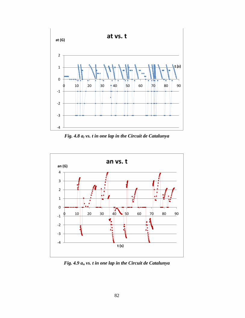
82

Fig. 4.8 at vs. t in one lap in the Circuit de Catalunya

Fig. 4.9 an vs. t in one lap in the Circuit de Catalunya

-4

-3

-2

-1

0

1

2

0 10 20 30 40 50 60 70 80 90

at (G)

t (s)

at vs. t

-4

-3

-2

-1

0

1

2

3

4

0 10 20 30 40 50 60 70 80 90

an (G)

t (s)

an vs. t

83

Finally, from this model calculation the time that the vehicle needed for covering a

complete lap was of 88.18 seconds. Such time will be then compared with the time that the

real race driver spent in the trajectory that is usually taken. For knowing more about how is

the real develop of the vehicle in this race-track, it is shown below the real behavior of the

vehicle within it.

4.2.2. The path taken by a Formula One Racer

Like the title says, in this point it is going to be treated the way how a Formula One race

driver affronted this race-track. For recollecting the data, there were installed

accelerometers and speedometers inside the vehicle for having the real behave of the

vehicle within the race-track having every moment that the data was recorded, nothing less

than real conditions.

All of these data was obtained by a remarked group of Engineers that work in the analysis

of the behavior of the vehicle during the race-track and who were responsible for making

an approximation to the behavior that the vehicle has during a race-track, by extracting the

real data of the variables of the vehicle and making a model that get closer to the behave of

them within the race-track, having done a complete investigation, resumed in a technical

note6 where is made an analysis between their model and the real life behavior of the

vehicle in the track of Barcelona.

The results obtained by the accelerometers and the speedometers were plotted and are

shown in the Fig. 4.10 which is below.

84

Fig. 4.10 Behavior of the variables of a Formula One vehicle while covering the Circuit

de Catalunya lap

Like it is shown in the last figure, the behavior of the centripetal acceleration (lateral

acceleration in the Figure 4.10) it is not represented by a constant line in the graphic,

instead of that it is represented by an erratic line that does not give a certainty of where is

located the centripetal acceleration in each moment of the lap. The velocity has a similar

behavior, but there is a more uniform line presented for this graphic. For the non-uniformly

line created in the last graphics, the engineers that were responsible of this investigation

made an approximation having like a final result a centripetal acceleration behavior that

could be smoothly represented and interpolated until it was obtained a uniformly line in the

graphic. The result obtained after they smoothed the behavior of the centripetal acceleration

of the vehicle is shown in the Fig. 4.11 which is below.

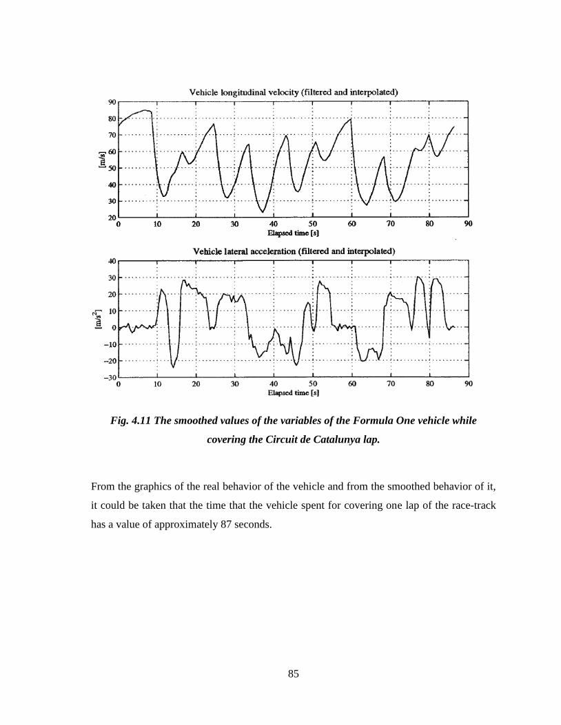
85

Fig. 4.11 The smoothed values of the variables of the Formula One vehicle while

covering the Circuit de Catalunya lap.

From the graphics of the real behavior of the vehicle and from the smoothed behavior of it,

it could be taken that the time that the vehicle spent for covering one lap of the race-track

has a value of approximately 87 seconds.

86

4.3. Comparison between the Path # 2 trajectory and the Formula One vehicle

trajectory

It could be noticed that if it is compared the behavior of the variables of the model and the

variables of the trajectory covered by the Formula One vehicle, it does not exist an equal

result, but there exist a certain similarity between each other, having similar behaviors

while each trace of the race-track is covered. About the times between each other, there

could be noticed that there was a difference between the times of the two trajectories of

Δt = 1.18s, being this a satisfactory result for the model, due it was made considering basic

physic equations for describing the movement of the vehicle within the race-track, having

also included the physical and geometrical restrictions for its calculations, concluding that

the Path # 2 model returns a closer approximation about how a high-performance vehicle

take the curves and gives to the persons interested into study this phenomenon, the

opportunity to have a good starting point tool that facilitates the calculation of the time of

the vehicle in whatever race-track, returning like a final answer a time that is really closer

with the time obtained by one the Formula One driver.

The final point of the comparisons in this point will be to compare the two trajectories and

to appreciate if they are closer enough or if it is mistaken to think that the model could be

approximated to the real life trajectory. For this comparison it is used the Figure 4.12,

which contains the real trajectory used by the Formula One driver accompanied by the

centerline of the Barcelona race-track and in the Figure 4.13 the model trajectory also

accompanied by the centerline of the Barcelona race-track. These both figures are shown

below.

87

Fig. 4.12 The trajectory traced by a Formula One driver

Fig. 4.13 The trajectory used in the Path # 2 model

88

In the last two figures the dotted lines, were the centerlines of the race-track and the solid

line of the figures were the trajectory of each one. Like it could be noticed, a same behavior

of trajectory was not obtained with the model, but certainly it is pretty similar with the real

trajectory, having like a final conclusion of this chapter that the program could actually be a

very useful and an easy to use tool for developing a first approximation about how the

displacement of the vehicle should be while its covering the race-track, considering also

that the times between the model and the Formula One driver trajectory are really close. It

should be also be have in mind that even that the results are closer enough like for using the

program like a starting tool, this Microsoft Excel program is just an approximation with a

some idealizations that tries to explain the real behave of a high performance vehicle, for

which the results obtained was satisfactory enough like for using it but for improving it, for

getting even more closer to the real results.

89

4.4. Annotations

1www.circuitcat.com

2http://galeria.forocoches.com/data/500/Montmel_.JPG

3 Appendix-B.

4 Fixed to the geometrical limits of the race-track.

5 The vehicle started by the rest, but the measure of its variables started with this value.

6 D Casanova, R S Sharp, P Symonds. Construction of race circuit geometry from on-car

measurements. ImechE. 2001.

91

CHAPTER 5. CONCLUSIONS AND RECOMMENDATIONS

5.1. CONCLUSIONS

This investigation was based in the fact that with the properly change of accelerations while

the vehicle is covering the race-track, there was going to be possible to obtain a trajectory

that was going to give the possibility to the race driver to achieve the lower time possible

for whatever kind of race-track. For getting this result, it was needed develop a model that

was going to be submitted to some restrictions, necessaries for having the closest

approximation possible to the real behavior that the high performance vehicle has in the

real life. The restrictions that were applied to the model were geometrical and physical,

having like geometrical restriction that the vehicle should cover the race-track inside of the

road and like physical restrictions that the vehicle will have some acceleration and velocity

limits that will mark the behave of the car in the race-track. Like acceleration limits there

was used the modified friction circle for having a restriction about between what values

should the total acceleration of the vehicle in whatever point of the vehicle be located in.

Now like velocity limits, it was considered that due it is being analyzed a high-performance

vehicle, its speed limits are located between 0 and 300 km/h

For concluding, it could be said that between the paths used for cover the race-track, the

best pattern was marked by the path # 2, due a program in Microsoft Excel was created for

trying to reach the best develop of velocities possible with the technique of “proof and

error” for which it could be assured that the high-performance vehicle will be always

working under the acceleration and velocity restriction, and that it will be always covering

the race-track within the road, having like a final guarantee that in the path # 2 it was

achieved a positive reduction in the lap-time of around five seconds, which is a huge

advantage if a race of a lot of laps (normally 50 or more in the common races that are done

nowadays) it is going to be realized.

92

5.2. RECOMMENDATIONS

The model that was finally developed in the path # 2 gives a very good idea about how the

behavior of the high-performance vehicle should be in a really race-track, nevertheless

there were made a lot of considerations for trying to model the behavior that the vehicle

should develop in the race-track, that still leaves the model like an approximation of what

should happened in the real life with the high performance vehicle. For improving the

behavior of the vehicle with the model created, fewer considerations should be done for

approximating more the model created with the real high-performance vehicle behavior.

It should be taken in count that for evaluating the path # 2, it was assumed that the bigger

radius possible was going to be used in each corner, considering changes of acceleration

and velocity in them. Like a recommendation for further investigations it could be

considered to evaluate different kind of curves that could develop a better behavior of

acceleration in the corners. It is really important to take in count this recommendation,

because if the corners are covered with a better behave of acceleration, then it will not only

be gained time in the corners, but also the straights will be covered with the better behave

of velocities possible, having like a final result a improve in the lap-time, which was since

the beginning the fundamental objective pursued in the present investigation.

93

GLOSSARY

Aerodynamics: Is a branch of dynamics concerned with studying the motion of air,

particularly when it interacts with a moving object.

Centripetal acceleration: Is the radial component of the acceleration of a particle or

object moving around a circle, which can be shown to be directed toward the center of

the circle.

Centripetal force: The component of force acting on a body in curvilinear motion that

is directed toward the center of curvature or axis of rotation. Centripetal force is

necessary for an object to move with circular motion.

Dynamics: The branch of mechanics that is concerned with the effects of forces on the

motion of a body or system of bodies, especially of forces that do not originate within

the system itself.

Geometry: A physical arrangement suggesting geometric forms or lines.

Physics: the branch of science concerned with the properties of matter and energy and

the relationships between them. It is based on mathematics and traditionally includes

mechanics, optics, electricity and magnetism, acoustics, and heat.

Speed: The rate or a measure of the rate of motion that is also the magnitude of the

velocity.

Tangential acceleration: The component of linear acceleration tangent to the path of a

particle moving in a circular path.

Tangential force: A force which acts on a moving body in the direction of a tangent to

the path of the body, its effect being to increase or diminish the velocity.

Velocity: The rate and direction of the change in the position of an object.

95

BIBLIOGRAPHY

Lopez, Carl. Going faster!, Mastering the Art of Race Driving. The Skip Barber Racing

School, 1997.

D Casanova, R S Sharp, P Symonds. Construction of race circuit geometry from on-

car measurements. ImechE. 2001.

Lee, Johns. The friction circle: The secret of vehicle control.

McIver, John. The GG Diagram. 1996.

Speranza Neto, Mauro. Class notes: Introduction to Engineering and Vehicle

Dynamics, 2009.

http://www.nwalfaclub.com/track/images/apex.gif

http://www.mgf.ultimatemg.com/group2/suspension/tracking.htm

http://www.mgf.ultimatemg.com/group2/suspension/tracking.htm

www.cicuitcat.com

http://galeria.forocoches.com/data/500/Montmel_.JPG

http://148.216.10.84/matematicas/cuerpo.htm

http://www.driftingstreet.com/racing-line-corner-layout.html

http://www.kalipedia.com/kalipediamedia/cienciasnaturales/media/200709/24/fisicayq

uimica/20070924klpcnafyq_133.Ges.SCO.png

http://upload.wikimedia.org/wikipedia/commons/thumb/1/19/Moglfm0410_component

es_aceleración.jpg/300px-Moglfm0410_componentes_aceleración.jpg

http://www.iihs.org/ratings/esc/esc_explained.html

http://www.mgf.ultimatemg.com/group2/suspension/tracking.htm

http://en.wikipedia.org/wiki/Circuit_de_Catalunya

APPENDIX A

THEORETICAL BASE

EXERCISES

A-1

THEORETICAL BASE EXERCISES

In this appendix is going to be explained some base exercises that was used for developing

the different trajectories that could be taken with the vehicle, so there could be used for

having an idea about how was the process of creating the ideal line. The exercises cover the

different variables that affect the behavior of different vehicles in different race-track

situation but there were useful for having a base before trying to reach a process for create

an ideal line.

The base exercises are shown and explained at below:

1. The Equations that describe the cinematic behavior of a vehicle, supposing that is a

particle with a mass m (kg), are given for

n

t

aV

adt

dV

1

In the ones, V is the linear velocity (m/s), at is the tangential acceleration (m/s2), is it

angular velocity (rad/s) and an is the centripetal acceleration (m/s2).

The acceleration profiles that are shown in the Figure A-1.1 were measured by a

telemetric system that was installed in the vehicle while it was covering a determinate

trace of a race-track.

A-2

Fig.

A-1.1 Acc. profiles of a car in a determinate point of the race-track

Considering that V(0) = 180 km/h and g = 10 m/s2, prove that:

a) The velocity of the vehicle in the position X=250 m is of 180 km/h.

b) Between 250 m and 550 m the vehicle is covering a corner with a radius of 180 m

Solution

a) Using the Equation 3.2 and using the initial data, the velocity of the vehicle in the

position X=250 m is obtained, considering that two different tangential accelerations

are going to be applied to the vehicle before reaching the position X=250 m. In the trace

one (the first 200 m) an acceleration of 1 G was applied; in the trace 2 (the following 50

m) a deceleration of -4 G was applied.

A-3

R//

So like was asked, with the changes of acceleration, the velocity in the position X=250

m has a value of V=180 km/h.

b) In the trace between X=250 m and X=550 m it could be noticed that there is only

applied a centripetal acceleration with a value of 2.5 G, what means that the vehicle in

that moment is in a corner with a constant velocity. So for finding the radius that the

vehicle is covering in the corner, considering that due the non change of tangential

acceleration the velocity of the vehicle in the corner has a value of V=180 km/h, the

Equation 1.4. was used.

R//

So it is concluded that the radius for the trace of the race-track between the positions

X=250 m and X=550 m it is correctly R=100m

A-4

2. In the Figure A-1.2 the vehicle A follow the trajectory a-a, while the vehicle B follows

the trajectory b-b, over a track without inclination. If each vehicle has a constant

limited velocity corresponding to a centripetal acceleration of 0.8 G, determine:

a) The times tA and tB which the ones the vehicles cover the corner delimited by the

line C-C

b) The velocities of the vehicles A and B in its corresponding trajectories.

c) The trajectory of the minimum time.

Fig. A-1.2 Trajectories in a predefined trace

Solution

a) There will be needed to obtain the velocity of the vehicles and the distances covered per

each vehicle at that constant velocity for determining the time of the vehicle in each

trace. So for determining the velocity of the vehicle in each trace was used the Equation

1.4 and for determining the time of the vehicle in each trace the Equation 3.6 was used.

A-5

The trace covered by each vehicle was:

The time that each vehicle spent in each trace was:

R//

R//

b) The velocity that was used to cover each trace was obtained before for calculating the

time that each vehicle spent in each trace, so the velocity of each vehicle is presented

below:

R//

R//

c) R// The trajectory that was made in the minimum time was the one covered by the

vehicle A, with a difference of time of 0.34 seconds between each other.

A-6

3. The Figure A-1.3 shows two possible trajectories that could be taken in a corner not

inclined in an horizontal trace of a race-track. The trajectory AA follows the central line

of the track and has a curvature radius of A = 85 m, while the trajectory BB uses parts

of the straights of the race-track having a good advantage for increasing the curvature

radius to a value of B = 200 m. If the pilots establish a limit for the velocities of the

vehicle in this corner, in a way that a centripetal acceleration of 0.8 G is not trespassed,

determine:

a) The maximum velocity for each trajectory.

b) The time that the vehicle needed to cover each trajectory.

c) The trajectory of the minimum time.

Fig. A-1.3Trajectories in a pre-defined trace

Solution

a) The maximum velocity for each trajectory was obtained with the Equation 1.4 which

the one is possible, knowing that each trajectory will have different radius, but that will

be covered at a same centripetal acceleration.

A-7

R//

R//

b) Like the vehicle will be covering the different trajectories with constant the velocities, it

is needed to obtain the length of the trace before calculating the time in each trace with

the Equation 3.6.

The trace that was going to be covered was:

The time that each vehicle spent in each trace with it constant velocity was:

R//

R//

c) R// With the calculation of the past literal it could be concluded that the trajectory in

which the vehicle spends the less time is the trajectory B, due the vehicle had a bigger

radius in this trajectory permitting to the vehicle to reach a higher velocity in the corner

for a result of a difference of time between the trajectories of 2.85 for the same corner.

A-8

4. Analyze the differences of velocity and time between the traces shown in the Figure A-

1.4

What is the value of the centripetal acceleration in each trace?

Fig. A-1.4 Different traces for a 90° corner

Solution

For each trace there will be used the Equation 1.4 for obtaining the maximal centripetal

acceleration that could be reached with the conditions of the vehicle in each trajectory.

Trajectory 1:

R//

A-9

Trajectory 2:

R//

Trajectory 3:

R//

Like it could be noticed, the minor centripetal acceleration was obtained in the corner

with the biggest radius due the centripetal acceleration is inversely proportional to the

radius of the corner, permitting to the vehicle to reach the higher velocity in the corner

with the biggest radius.

A-10

5. Analyze the differences in the traces of velocity and time between the trajectories

shown in the Figure A-1.5 for a “S corner”.

In which trace is obtained the minor time?

What is the value of the centripetal acceleration in each part of each the trace?

Fig. A-1.5.a Trace 1 for a S Curve

A-11

Fig. A-1.5.b Trace 2 for a S Curve

Fig. A-1.5.c Trace 3 for a S Curve

A-12

Fig. A-1.5.d Trace 4 for a S Curve

Solution

In this exercise it is shown the different paths that could be taken for minimizing the time in

the S Curve. Due each path has been covered with a different behavior of acceleration, then

there will be separately explained for a better comprehension of it solution. The paths are

explained at below:

a) The 1st path was divided in two mini paths with the following characteristics:

Mini-path a: Has a constant radius of R=46.02 m and a constant speed of

V=21.11 m

/s and is the first arc of circle of the S Curve.

Mini-path b: Has a constant radius of R=62.79 m and a constant speed of

V=24.71 m

/s and is the second arc of circle of the S Curve.

The centripetal accelerations of each mini-path were obtained with the Equation 1.4 and

are shown below:

A-13

R//

R//

Like it does not exist a change of velocity in the corners the times in each was taken

with the next formula:

The total time spent in the corner was the sum of the time spent in the mini-path a, with

the time spent in the mini-path b.

R//

b) The 2nd

path was divided in two mini paths with the following characteristics:

Mini-path a: Has a constant radius of R=49.68 m and a constant speed of

V=21.96 m

/s and is the first arc of circle of the S Curve.

Mini-path b: Has a constant radius of R=62.79 m and a constant speed of

V=24.71 m

/s and is the second arc of circle of the S Curve.

A-14

The centripetal accelerations of each mini-path were obtained with the Equation 1.4 and

are shown below:

R//

R//

Like it does not exist a change of velocity in the corners the times in each was taken

with the next formula:

The total time spent in the corner was the sum of the time spent in the mini-path a, with

the time spent in the mini-path b.

R//

c) The 3rd

path was divided in two mini paths with the following characteristics:

Mini-path a: Has a constant radius of R=46.02 m and a constant speed of

V=21.11 m

/s and is the first arc of circle of the S Curve.

A-15

Mini-path b: Has a constant radius of R=62.79 m and an initial velocity of

V=20.89 m

/s with a final velocity of V=22.67 m

/s and is the second arc of circle

of the S Curve. This mini-path will count with a change of velocity while its

covering the corner, so in this case it will exist a variable centripetal acceleration

and a constant tangential acceleration. The variable centripetal acceleration will

exist due the velocity is changing in the curve, so it was no calculated the

centripetal acceleration for the second part of the S Curve.

The centripetal accelerations of the mini-path a, was obtained with the Equation 1.4 and

is shown below:

R//

Before calculating the times of each mini-path it should be obtained the tangential

acceleration of the second mini-path, which was calculated with a variation of the

Equation 3.2, that is shown below.

In the first part of the S Curve it does not exist change of the velocity, so the time that

the vehicle spent was in that part of the track was calculated with the Equation 3.6, and

was of:

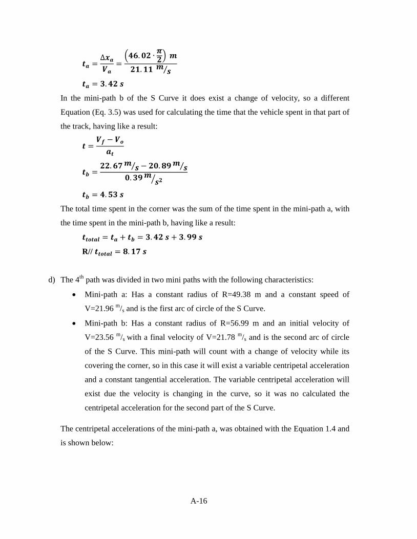
A-16

In the mini-path b of the S Curve it does exist a change of velocity, so a different

Equation (Eq. 3.5) was used for calculating the time that the vehicle spent in that part of

the track, having like a result:

The total time spent in the corner was the sum of the time spent in the mini-path a, with

the time spent in the mini-path b, having like a result:

R//

d) The 4th

path was divided in two mini paths with the following characteristics:

Mini-path a: Has a constant radius of R=49.38 m and a constant speed of

V=21.96 m

/s and is the first arc of circle of the S Curve.

Mini-path b: Has a constant radius of R=56.99 m and an initial velocity of

V=23.56 m

/s with a final velocity of V=21.78 m

/s and is the second arc of circle

of the S Curve. This mini-path will count with a change of velocity while its

covering the corner, so in this case it will exist a variable centripetal acceleration

and a constant tangential acceleration. The variable centripetal acceleration will

exist due the velocity is changing in the curve, so it was no calculated the

centripetal acceleration for the second part of the S Curve.

The centripetal accelerations of the mini-path a, was obtained with the Equation 1.4 and

is shown below:

A-17

R//

Before calculating the times of each mini-path it should be obtained the tangential

acceleration of the second mini-path, which was calculated with a variation of the

Equation 3.2, that is shown below.

In the first part of the S Curve it does not exist change of the velocity, so the time that

the vehicle spent was in that part of the track was calculated with the Equation 3.6, and

was of:

In the mini-path b of the S Curve it does exist a change of velocity, so a different

Equation (Eq. 3.5) was used for calculating the time that the vehicle spent in that part of

the track, having like a result:

A-18

The total time spent in the corner was the sum of the time spent in the mini-path a, with

the time spent in the mini-path b, having like a result:

R//

APPENDIX B

CONSIDERATIONS FOR

USING THE MICROSOFT

EXCEL PROGRAM

B-1

CONSIDERATIONS FOR USING THE MICROSOFT EXCEL

PROGRAM

Some considerations must be taken before running the Microsoft Excel program that is

responsible of evaluating the model of the path # 2 of the present investigation. These

considerations must be followed for having the program running with the best behavior

possible and are explained below:

The first consideration that should be taken is that the straights will always

be located between two corners, because for changing of straight it is needed

to take a corner, so it is confirmed that this consideration it is needed for

having the closer approximation to the real life behave.

The next consideration is that the final velocity of each straight should be

equal or lower than the initial velocity of it, trying to have the minimum

delta of velocity between these two values. This consideration is made due it

is not known how long will be the length of each straight, so condition was

assumed for having a good develop of the program and for reaching a

correct response from the program. Now, this consideration it is not assumed

for the first trace of the track (that usually is a straight of the race-track)

because the vehicle part from the rest (with a velocity equal to zero), having

always a higher velocity at the end of that straight, for which the condition

could not be used.

There will exist some places in the race-track where will exist the necessity

of take a corner after other corner and for these situations it will be needed to

use like initial velocity of the second corner, the final velocity of the first

corner for having a logical continuity of velocity of the vehicle.