Detention and mixing in free water wetlands

ELSEVIER Ecological Engineering 3 (1994) 345-380

ECOLOGICAL ENGINEERING

Detention and mixing in free water wetlands

R o b e r t H. Kadlec

The University of Michigan, Department of Chemical Engineering, Ann Arbor, MI 48109-2136, USA

Received 18 June 1993; accepted 10 February 1994

Abstract

Mixing was studied in a free water surface wetland receiving pumped river water, by measurement of the non-interacting tracer lithium. The flow pattern was found to be intermediate between plug flow and well-mixed. The nominal detention time, calculated from volume and flow, was 50% larger than the mean tracer detention time. The peak time was found to be one-half the tracer detention time. Three models were constructed: plug flow with dispersion, tanks in series, and a series-parallel network of tanks. All proved capable of fitting the exit tracer concentration curves but the network model provided a better fit to internal measurements. Pumping frequency was high enough to allow use of an average flowrate. The degree of mixing, as characterized by the variance of the exit tracer response curve, was comparable to that found by other researchers for wetlands, ponds and rivers.

Keywords: Detention time; Flow modeling; Hydrology; Mixing; Tracer testing; Wetlands

I. Introduction

Wetlands are finding increasing applications as potential chemical transformation systems for a wide variety of water-borne contaminants. This branch of ecological engineering has borrowed heavily from the concepts and practices of environmental engineering. Environmental engineering has in the past relied upon simplistic descriptions of the rates of transformation, reduction and removal of pollutants from water in various ecosystem settings. The assumptions of first order removal kinetics and plug flow or well-mixed water movement have typified models of transport and conversion. However, these presumptions are often only expedi- ent choices made because of a lack of system-specific information.

Constructed wetland ecosystems now number in the hundreds in each of several

0925-8574/94/$07.00 © 1994 Elsevier Science B.V. All rights reserved SSDI 0925-8574(94)00007-R

346 R.H. Kadlec /Ecological Engineering 3 (1994) 345-380

application categories and wetland types. Design of such ecosystems is a maturing science, which seeks to pinpoint the parameters of each new project within ever-narrowing bounds. Prediction and simulation of fate and transport of contaminants in a wetland requires modeling of processes in an existing ecosystem. Design of a constructed wetland utilizes those same models, but also requires knowledge of the influence of configuration and community structure on those processes.

Ecological process descriptions are complex, and therefore deservedly receive close scrutiny within each application category (Mitsch and Gosselink, 1993; Reddy and D'Angelo, 1994). Soils, sediments, microbes and macrophytes may all play important roles in removal mechanisms.

But first and foremost, it is necessary to understand the movements of water within the wetland. Process descriptions must involve hydrologic parameters at some level. The concepts of detention time and hydraulic loading rate may suffice to develop site-specific correlations of output versus input, but such correlations require extensive replication to define the variability due to site parameters. Unfortunately, the very popular and simple "first order model", when based solely on input and output information under invariant operating conditions, is nothing more than a variant of this correlation technique.

There is a very large body of knowledge, both experimental and theoretical, that has evolved from the necessity to design chemical reactors for the chemical, petrochemical, and biochemical process industries. The discipline of chemical reaction engineering has matured to the point that this information is standard in many textbooks, which address several levels of audiences (see e.g., Levenspiel, 1972; Fogler, 1992). Standard procedures are available for the blending of hydro- dynamics and intrinsic chemical or biochemical process rates. The principal ingredients of these procedures are the development of models for flow from tracer tests and mass balances, and the development of localized models of chemical interactions. In concrete-and-steel process reactors, flow models may often be inferred from past research and the geometry of the system, and operating conditions, such as flow rate and reactor volume.

There is now a need to develop similar understanding of wetland reactors. That need is based on the inefficiency of inter-site correlation as a means of explaining the abiotic processes of wetland hydrology and its influence on pollutant removal.

The traditional chemical reaction engineering literature is divided into several categories on the subjects of flow (hydrology) and mixing. Ideal mixing pattern limits are considered to be fully mixed (continuous stirred tank reactors = CSTRs) and plug flow (plug flow reactors = PFRs). Reactors are considered to be homogeneous if there are no chemically active solids present; or heterogeneous if there are chemically active solid surfaces present. Mass transfer limitations are inten- tionally minimized. Most process reactors are designed for steady flow operation at one extreme, or batch processing at the other extreme. Mass balances for the inert carrier (water) are generally not required. Flows are preset to be either laminar or turbulent. Designs are often set so that some set of these limiting conditions is met; based on an understanding of what the process chemistry requires and a knowledge of how to achieve the limiting conditions. For instance, a frequent

R.H. Kadlec / Ecological Engineering 3 (1994) 345-380 347

choice in the chemical industry is the steady state, heterogeneous plug flow reactor.

It is becoming apparent from a variety of research projects that wetland reactors do not fit any of these limiting conditions. They are intermediate between CSTR and PFR behavior, as this study shows. The flows are typically in the transition region between laminar and turbulent (Kadlec, 1990). They may receive a steady input flow, but they are not steady state because of meteorological phenomena. The chemistry is typically complex, involving biological reactions and mass transfer.

The objectives of this work are to introduce the concepts of non-ideal flow and mixing to wetland analysis, and to show that mixing is intermediate between plug flow and completely mixed. This paper illustrates techniques of description of wetland interior flow phenomena, and sets forth some results for a riverine wetland water quality improvement project.

1.1. RTD literature and theoretical background

The ideas used here were first proposed by Danckwerts (1953) who used the residence time distribution (RTD) to characterize chemical reactors. More recently, the theory of residence time distributions is elucidated in the textbooks of Levenspiel (1972) and Fogler (1992). These basic chemical reaction engineering principles can be applied to wetlands, since these are in fact chemical reactors. The residence time distribution represents the time various fractions of fluid (water in the case of the wetland) spend in the reactor, and hence is the contact time distribution for the system. In a broader context, the RTD is the probability density function for residence times in the wetland. This time function is defined by:

E ( t ) At = fraction of the incoming water which stays in the wetland

for a length of time between t and t + A t, (1)

where E = RTD function, 1/day; and t = time, day. The RTD function may be measured by injecting an impulse of dissolved inert

tracer material into the wetland inlet, and then measuring the tracer concentration as a function Of time at the wetland outlet. For an impulse input of tracer into a steadily flowing system, the function [E(t)] is:

OeC(t) C(t) E(t) = , (2)

o o

fo OeC(t) at fo c( t ) dt

where C(t) = exit tracer concentration, g/m3; and Qe = water flow rate, m3/day. The first numerator is the mass flow of tracer in the wetland effluent at any time t after the time of the impulse addition. The first denominator is the sum of all the tracer collected and thus should equal the total mass of tracer injected. The tracer concentration can be measured at interior wetland points as well as at the outlet.

348 R.H. Kadlec / Ecological Engineering 3 (1994) 345-380

Eq. 2 may then be used to determine the distribution of transit times to that internal point. In this broader sense, the RTD becomes a function of internal position, E(x, t ).

Unfortunately, most wetlands do not operate as steady state systems. For example, the flow rate is affected by pulsed pumping events, rainfall and evaporation. To account for the dynamic behavior, E(t) may be expressed in terms of mass instead of concentrations, as indicated by the first equality in Eq. 2.

Since the term E( t )A t represents the fraction of tracer that spends between time t and t + At in the system, the sum of these fractions is unity:

fo E ( t ) dt = 1. (3)

The moments of the RTD define the key parameters which characterize the wetland; the two most important being the actual detention time and the spreading of a concentration pulse due to mixing (variance of the pulse). The first absolute moment is the tracer detention time (~'a), which is the average time that a tracer particle spends in the wetland. This average time is also called actual residence time:

c~

= fo tE( t ) dt. (4) T a

Most of the literature on wetland hydrology defines a nominal residence time (also called the detention time) to be the ratio of the volume of water in the wetland divided by the volumetric flow rate of water through the wetland:

= V / Q , (5)

where V = volume of water in the wetland, m3; and ~- = nominal residence time, day.

A wetland may have excluded zones, which do not interact with flow, such as the volume occupied by plant materials. In a steady state system without excluded zones, the tracer detention time ( r a) equals the nominal residence time (r). This is true whether the flow patterns are ideal (plug flow or well-mixed), or nonideal (intermediate degree of mixing). In a dynamic wetland system, the nominal residence time would typically be defined as the ratio of the average water volume divided by the average water flow rate. However, in this situation, the nominal and mean residence times are usually not equal.

A second parameter which can be determined directly from the residence time distribution is the variance (or2), which characterizes the spread of the tracer response curve, or E-curve, about the mean of the distribution, which is %. This is the second central moment:

~r 2 = f o ( t - ~'a)2E(t) dt , (6)


where tr 2 = RTD variance, day 2. The variance of the RTD is created by preferen- tial flow paths and mixing of water during passage.

One measure of wetland performance is the extent of pollutant decomposition. The conversion of a reactant in any reacting system is defined as:

x = 1 - C/Co, (7)

where C = outlet reactant concentration, g/m3; and C O = inlet reactant concentration, g / m 3. The average conversion in a steady flow wetland can be found from the residence time distribution and batch reaction kinetics. For example, the conversion in a first order, homogeneous batch reaction is given by:

C / C o = 1 - x = e x p ( - k t ) , (8)

where k = reaction rate constant, day- l ; t = reaction time, day. This conversion is then averaged over the distribution of residence times within the actual wetland to yield:

0 o o o

X = £ x ( t ) E ( t ) d t = l - £ e x p ( - k t ) E ( t ) d t , (9)

where X = average conversion. Note that [x(t)E(t)dt] represents the conversion of the reactant fraction spending between time t and t + At in the system.

Clearly, the knowledge of E(t) permits the adaptation of simple kinetic expressions to the non-ideal flow patterns in a wetland for the prediction of average behavior in the steady flow system. However, transient flow patterns, with the accompanying transient storages of water and pollutants, would require transient RTD functions, which may differ depending upon the nature of the time-varying forcing functions. Transient RTD functions for the Des Plaines River wetlands are quite complex, as shown by Kadlec and Bastiaens (1992). It is therefore convenient to construct a flow model which embodies the measured RTD and the dynamic hydrological mass balance for water. There is then the possibility of capturing the major features of the dynamic flow patterns while preserving fairly simple calculation methods.

There are dozens of published methods for constructing such flow models (see the review of Call (1989), for example). Many of these consist of series and parallel combinations of the two ideal extremes of mixing: totally mixed zones (corresponding to a continuous stirred tank reactor or CSTR in the reaction literature) and totally unmixed zones (corresponding to a plug flow reactor or PFR in the reaction literature). The PFR may in turn be represented by an infinite series of CSTRs, or approximated by a smaller number, usually less than ten (Levenspiel, 1972). The end result is a that a series-parallel network of CSTRs is one of the possible representations of a non-ideal flow pattern, and is adopted in this work. A variation on this theme is the use of a dispersion process superimposed on a plug flow model. The dispersion coefficient is derivable from the variance of the tracer response.

350

2. Methods

R.H. Kadlec / Ecological Engineering 3 (1994) 345-380

2.1. Site description

Wetlands were constructed at a site on the Des Plaines River in northeastern Illinois, USA, for the purpose of demonstrating their potential for river water quality improvement. The basins were excavated and planted in 1987-88, and scheduled pumping of river water through four wetlands began in 1989. Extensive research has been conducted since that time, on all aspects of system function: hydrology, water quality, soils and biota. A more extensive description of these wetlands may be found in WRI (1992) and Hey et al. (1994).

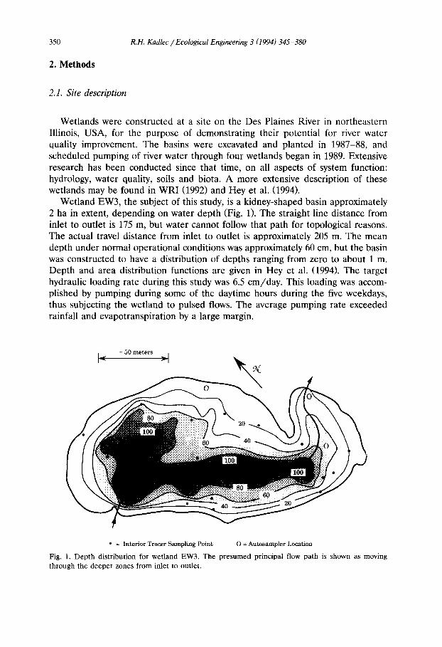
Wetland EW3, the subject of this study, is a kidney-shaped basin approximately 2 ha in extent, depending on water depth (Fig. 1). The straight line distance from inlet to outlet is 175 m, but water cannot follow that path for topological reasons. The actual travel distance from inlet to outlet is approximately 205 m. The mean depth under normal operational conditions was approximately 60 cm, but the basin was constructed to have a distribution of depths ranging from zero to about 1 m. Depth and area distribution functions are given in Hey et al. (1994). The target hydraulic loading rate during this study was 6.5 cm/day. This loading was accom- plished by pumping during some of the daytime hours during the five weekdays, thus subjecting the wetland to pulsed flows. The average pumping rate exceeded rainfall and evapotranspiration by a large margin.

]~ = 50 meters ~]

• = Interior Tracer Sampling Point O = Autosampler Location

Fig. 1. Depth distribution for wetland EW3. The presumed principal flow path is shown as moving through the deeper zones from inlet to outlet.


I .~ = 50 meters ~ I I~ r l

. . .

[ ] C a t t a i l ~ Floating Leaved ~ ' - ] Algae I IOp~nWat~r

=50meters ~1

Cattail ~ LeavedFl°ating I ]Algae I I Open W a t e r

Fig. 2. Principal vegetation types and distribution for wetland EW3, for (a, top) August 1, 1990 and (b, bottom) July 23, 1991. Interpreted from aerial color and color infrared photography and ground truth.

Vegetation patterns were slightly different in 1990 and 1991, which comprised the study period (Fig. 2). There was a slight decrease in the extent of cattail (Typha spp.) from 1990 to 1991, due in part to the activity of beavers and muskrats. There was an increase in the percent cover of floating leaved aquatic plants, mostly water


lily, Nymphea odorata (Fennessy et al., 1994). Filamentous green algae dominated a good share of the deeper water areas in both years, but the spatial distribution was different in the two years.

2.2. Hydrology

A water budget for wetland EW3 was available from the site, stored on a database. This included hourly values of inflow, outflow, precipitation, evapotranspiration (ET), seepage and simulated water levels. The overall water budget is dynamic in nature due to the discontinuous pumping, as well as the variability in rain and ET. Details are given by Hey et al. (1994).

The flow rate of river water into the wetland basins was tracked electronically by automated flow measuring sensors. Precipitation was measured using a rain gauge at the site. Evaporation was estimated from a modified Penman equation, which in turn relies upon weather data recorded at the site. Complete hydrologic budgets were prepared for the wetlands, including seepage (Hey et al., 1994). Seepage of water either into or out of EW3 was considered negligible for the duration of the tracer experiments; for instance, it comprised 0.12% of the inflow for the tracer test period in June 1991. The outflow from EW3 was determined from a stage-discharge calibration of the exit weir. Calibration was performed with a factory-calibrated turbine flow meter. Water levels were then calculated from the dynamic water mass balance equation.

This water budget was reprogrammed for purposes of this study because of the necessity of coupling the dynamic tracer mass balance equations to the dynamic water mass balance. This computer code utilized all but the discharge rates and simulated water levels from the site database. The discharge rate was thus determined from a modification of the Francis weir formula (Perry and Chilton, 1973):

Qe(t ) = / 3 [ h o ( t ) ] ,.5, (10)

where Q e ( t ) = o u t f l o w rate, m3/day; ho ( t )=he igh t over the weir, m; /3 = calibration constant, ml5 /day .

The discharge calibration did not extend to low water levels ( < 6 cm over the weir). This leads to some uncertainty in the accuracy of the weir formula during periods when basin levels were in this range. For EW3, /3 = 55.25 × 103 fit the 1991 experimental outflow values to within an average of 5.7%.

The basin water level was calculated from the dynamic mass balance for the wetland (see Fig. 3):

d ( A h ) dt - QP - Qe + A( P - E T ) ' (11)

where A = water surface area, m2; ET = evapotranspiration, m / d a y ; h = water elevation above datum, m; P = precipitation, m / d a y ; Qp = pumping rate, m3/day; t = time, day.


Evapotranspira t ion = ET Precipitation = R

,. '

L Surface Area = A

Fig. 3. G e n e r a l t e r m i n o l o g y a n d c o m p o n e n t s o f the w a t e r mass b a l a n c e .

The wetland bot tom topography was determined from a site survey, which in turn determined the water surface area at several water elevations. The d e p t h - a r e a distribution function is given in Hey et al. (1994). The surface area at and above weir elevations was essentially constant. The differential water balance was solved using a fourth order Runge -Ku t t a routine on a spreadsheet.

The total volume of water in the wetland is comprised of the volume above the weir and the volume below the weir. Wetland EW3 does not have a level bot tom (Fig. 1), and hence depth varies with location. The total volume below the weir was calculated from the basin topography. The mean depth below the weir is defined a s :

hw=VwA, (12)

where V w = water volume below weir, m3; h w = depth below the weir, m. The total depth to the mean bot tom elevation is:

h = h o + h w. (13)

The total water volume is:

V = hA. (14)

2.3. Tracer studies

Preweighed samples of lithium chloride were dissolved in Des Plaines river water in 150-1 plastic waste cans near the basin inlet. The resulting solution was dumped into the wetland inlet when the pump was on. To insure maximum mixing, the contents and subsequent rinse waters were poured directly into the turbulent zone at the pipe discharge point.


0.241 I ho model

0.211 * ho experimental /

0.18-~

~ '$ 0.15-

0 1 2

~. 0.09-

0.06 -

0.03 -

0 . 0 0 . . . . , . . . . , . . . . , . . . . , . . . . . . . . . , . . . . , . . . . , . . . . 0 5 10 15 20 25 30 35 40 45

Time, days

Fig. 4. Dynamic water elevations in wetland EW3 for the period June 3-July 16, 1991.

Samples were collected every 2 h at the wetland outlets using automatic samplers with 500-ml glass bottles. A 10-ml subsample was transferred to glass vials, previously acid washed, rinsed with deionized water, and rinsed with the sample solution.

Lithium analysis was performed via atomic absorption spectrophotometry. Stan- dard solutions containing 0.01, 0.1, 0.5 and 1.0 mg/1 lithium were made to calibrate the spectrophotometer. Five replicate absorption values were taken of each of the wetland samples and then averaged. The average standard deviation for two of the tracer runs was 0.0023 mg/1 (n = 2875). The detection limit for the instrument was approximately 0.001 mg/ l .

3. Results and discussion

3.1. Hydrology

The transient behavior of the wetland water level is shown in Fig. 4. The results are shown for a 45-day period in June of 1991 during which time a tracer test was taking place. The sharp peaks result from the pump being turned on for only 4 h per day. The water levels above the weir, h o, simulated using Eqs. 11-13, were accurate to within about 5 to 25% of measured values depending on the time period involved (Table 1). The measured values were recorded on site twice a day during weekdays. The five time periods listed in the table represent the duration of individual tracer tests conducted at the site. In August 1991, the average water level is in the uncertain range of the weir formula. If the height below the weir (h w) is included in the water level, errors are reduced significantly. However, the


Table 1 Water mass balance errors, wetland EW3. Mean depth=0.621_+0.015 m. Errors are differences between data and simulation

Run Height over weir Average error % error in h o % error in h Data average h o (m) (m) Height over weir Mean depth

Oct-90 0.101 0.006 5.9 1.0 May-91 0.094 0.018 18.2 2.9 Jun-91 0.101 0.006 7.3 1.0 Jul-91 0.098 0.009 9.8 1.5 Aug-91 0.064 0.015 23.5 2.5

Average 12.9 1.8

accuracy of the outflow rate is directly affected by the height over the weir (Eq. 13), and errors in h o propagate to the outflow (Qe).

3.2. Tracer studies

Tracer selection A non-reactive, soluble material is required for tracer studies. The tracer is

required to move with the water, and it is necessary that the tracer not react with or adsorb to any ecosystem component, such as soils, sediments, litter or vegetation. Comparative wetland studies (Netter and Bischofsberger, 1990; Pauly et al., 1990) demonstrated that bromine, lithium, and fluorescein dyes are all approximately equivalent for this purpose. Lithium was demonstrated to not sorb to wetland soils and sediments associated with wetland EW3. Laboratory tests involving exposure of soils and sediments to lithium chloride in solution yielded 98.4 + 3.3% (N = 30) recovery in the water phase.

The fluorescein dye Rhodamine B was also used in wetland testing, but was found to sorb significantly to wetland particulate materials in laboratory tests. Its use was subsequently discontinued. This finding is supported by other studies; for instance, Egger (1992) found that peat sorbed nearly all of the added Rhodamine at shallow water depths.

Tracer response curves The lithium exit concentration distributions were determined for wetland EW3

during several tests spanning the pumping seasons of 1990 and 1991. A typical response curve is bell shaped with a long tail (Fig. 5).

Tracer mass balances The lithium mass balance was checked, by comparing the added lithium to the

total lithium found in the exit flow. The total mass of lithium exiting a wetland during a test is given by:

M o = f t f O e ( t ) C ( t ) d t , (15) J0


%

o

0 . 4 0 "

0.35 "

0.30 "

0.25 •

0.20 "

0.15 '

0.10 •

0.05 •

0.00 . . . . i . . . . i . . . . ! • .

5 10 15 20 25

Time, days

Fig. 5. Lithium tracer response curve at the exit of wetland EW3 for the period July 16-August 10, 1991.

where M o = outflow lithium mass, g; tf = total time span of the outflow pulse, day. Eq. 15 defines Mo, the zeroth moment of the tracer flow distribution. The value of t f must be sufficiently high so that the tracer has totally flushed from the wetland.

[~1 o -- Q. foeC( t ) dt, (16)

where 0 = mean outflow, m3/day; Mo = zeroth moment based on mean outflow, g.

Eq. 16 is based on the approximation of the mean of the product equaling the product of the means for flow and concentration. This assumption was found to be

Table 2

Tracer mass balances, in g lithium, based on average flow, and on dynamic flow

Run Input Output Output

(mean flow) (dynamic flow)

Aug-90 1663 1483 Oct-90 5760

May-91 1606 a Jun-91 4125 4139 Jul-91 2695 3261 Aug-91 2673 2298 Oct-91 2670 2490

Average 2572 2734 Average 3164

Recovery 106%

6240 a

4560 3030 1490 b

3027

96%

Analytical problems. b Not modeled; ice blockage at outflow.


valid to within less than 1% for a typical tracer test. It avoids the expense of close interval outflow measurement. For wetland EW3, the net water loss due to evapotranspiration minus precipitation was 1% in 1990 and 3% in 1991 (Hey et al., 1994). Consequently, Q could be determined from the pumping rate and duration.

The calculation of 3~ o is sensitive to the long "tail" of the concentration response curve. Curl and McMillan (1966) found that such tails are well represented by an exponential decay. Therefore, truncated data which terminated too early were extrapolated to zero concentration via an exponential decay.

The recovery of lithium averaged 96 _+ 14% based on Eq. 15, and 106 _+ 32% based on Eq. 16 (Table 2). The August 1991 mass balance did not close well (44% missing), suggesting that all of the lithium did not exit the basin. Since the lithium concentration had tapered off by the time this test ended, the run was not prematurely stopped. A possible cause of the inaccuracy of Eq. 15 for this test was the low August water levels. During more than half of this test, EW3 operated at levels below 6 cm over the weir, for which there was not direct calibration data.

Tracer detention time The tracer detention times for tracer runs were calculated from the defining

Eqs. 2 and 4:

where

£tftQe( t )C( t ) dt M1

Ta = f ( i fQe(t)C(t) dt - M~°' (17)

M 1 = fo f tQe( t )C( t ) dt, (18)

Eq. 18 defines M1, the first moment of the tracer flow distribution. It is convenient to utilize the average flow rate in the computation of M 1, for the reasons given above for /~0. That means approximating the first moment of the tracer flow distribution according to:

M1 = O. fot'tC( t ) dt, (19)

where 11~ 0 = first moment based on mean outflow, g. day. There arc three ways to calculate the detention time in the wetland: from wetland volume and average flow, from dynamic tracer and flow measurements (Eqs. 17 and 18), and from dynamic tracer and average flow measurements (Eqs. 16, 17 and 19). These are compared in Table 3.

It is clear from Table 3 that the nominal detention time is about 50% larger than the tracer detention time. The inference is that about one-third of the wetland volume is not involved in tracer movement. That in turn is presumably due to space occupied by stems and litter, as well as to zones which do not exchange water with the main flow on the time scale of several weeks.


Table 3 Detention times in days. Nominal time based on 1992 topography. Predicted mode is for n CSTRs

Run Nominal Tracer Tracer Nominal: Nominal: Mean: Mode Mode: Predicted (= V/Q) (mean (dynamic mean dynamic dynamic mean mode: mean

flow) flow)

Aug-90 10.43 6.60 6.17 158% 169% 1.07 4.5 68% 65% Oct-90 8.95 6.99 6.22 128% 144% 1.12 1.6 23% 64% May-91 9.19 8.20 ~t 112% ~ 1.7 Jun-91 9.73 6.36 7.04 153% 138% 0.90 3.5 55% 46% Jul-91 10.54 7.35 7.36 143% 143% 1.00 3.1 42% 57% Aug-91 24.55 12.45 11.12 197% 221% 1.12 6.9 55% 77% Oct-91 12.61 13.40 b 94% b 6.8 51% 54%

Average 149% 163% 1.04 49% 60%

a Analytical problems. b Not modeled; ice blockage at outflow. Excluded from average.

It is also possible that the wetland bottom topography is not correct, which may result from three sources of error. The first source is inaccuracy in the survey of the wetland bottom, which was conducted at the completion of construction, and again after three year's operation. The second error may be the datum elevation of the wetland bottom. The third potential error is the possibility of volume loss due to sediment accretion from internal and external sources. Surveying errors may be serious: two surveys of EW3 differed by 33% in wetland volume. The erroneous survey resulted in a volume so small that the tracer detention time exceeded the nominal detention time, thus requiring a volume correction (Kadlec and Bastiaens, 1992).

The use of a mean flow approximation seems to be justified for the flow schedules in this study. The detention times determined by the two techniques are not significantly different (significance level a = 0.05). The ratio was 1.04 + 0.09.

The time for the peak of the tracer to reach the outlet is by definition the mode of the concentration distribution. This peak time averaged 49% of the mean detention time (Table 3), and only 30% of the nominal detention time.

Tracer mixing The variance of the tracer response curve corresponds to the degree of mixing

in the wetland. The variance is a measure of the spreading of the concentration pulse after travel through the wetland. Eqs. 2 and 6 may be used to calculate 0-2:

0 -2 = fo"(t - "Ca)2Qe(t)C(t) dt

/ ' Q e ( t ) C ( t ) d t

where:

M 2 = f / f t 2 Q e ( t ) C ( t ) dt .

M 2 M~

M 0 M02 , (20)

(21)

R.H. Kadlec / Ecological Engineering 3 (1994) 345-380

Table 4 Wetland and depth dispersion numbers

359

Run z actual Exit pulse Normalized Wetland Dispersion Number of Depth (day) variance var iance dispersion constant well-mixed dispersion

tr 2 ~r02 number D sections number (day 2) D / uL (m2 / day) n D / uh

Aug-90 6.60 15.4 0.354 0.228 1464 2.8 77.05 Oct-90 6.99 17.8 0.364 0.238 1438 2.7 80.16 May-91 8.20 25.6 0.380 0.253 1303 2.6 85.22 Jun-91 6.36 22.0 0.545 0.461 3067 1.8 155.52 Jul-91 7.35 23.5 0.434 0.309 1777 2.3 104.15 Aug-91 12.45 35.2 0.227 0.131 444 4.4 44.11 Oct-91 13.40 83.6 0.465 0.233 735 2.2 78.54

Mean 31.9 0.396 0.264 1461 2.7 89.2 Standard deviation 23.7 0.100 0.101 843 0.8 34.2

Eq. 21 defines M 2, the second moment of the tracer flow distribution. It is convenient to utilize the average flow rate in the computation of M2, for the reasons given above for M 0. That means approximating the second moment of the tracer flow distribution according to:

)~12 = Q foqt2C( t ) d t , (22)

where 2Q 2 = second moment based on mean outflow, g" day. Variances calculated from Eqs. 16, 19, 20, and 22 range from 15 to 83 day 2 (Table 4). This range indicates an intermediate degree of mixing, between plug flow and a CSTR.

Replication o f field tracer tests Autosampling was performed at two locations inside wetland EW3 (Fig. 1) for

the tracer run of August, 1990. Results for samples taken at station 3a, located 75% of the way to the outlet along the main flow path, were satisfyingly similar to those for samples taken at station 3 at the wetland outlet, and provide confidence in the test and sampling procedures. At station 3a, 96% of the wetland volume was upstream; and the measured detention time was 6.32 days, or 96% of the detention time to the outlet (6.60 days).

Rhodamine B as a tracer Rhodamine B was also evaluated as a tracer. A dual pulse injection was made

into wetland EW3 (Urban, 1990), and the resultant concentrations of lithium and Rhodamine B were determined at the outlet in timed samples. Lithium was measured in the laboratory as specified previously. Rhodamine B was measured using a spectrofluorimeter (detection limit 1 rig/l). For the August, 1990 test, 159 triplicate samples were analysed for rhodamine, and 159 quintuplicate samples were analysed for lithium.


I ~ Rhodamine B, ppb

15 • ~ 100*Lithium, ppm

~ 13"

0 ' 0 5 10 15 20

Time, days

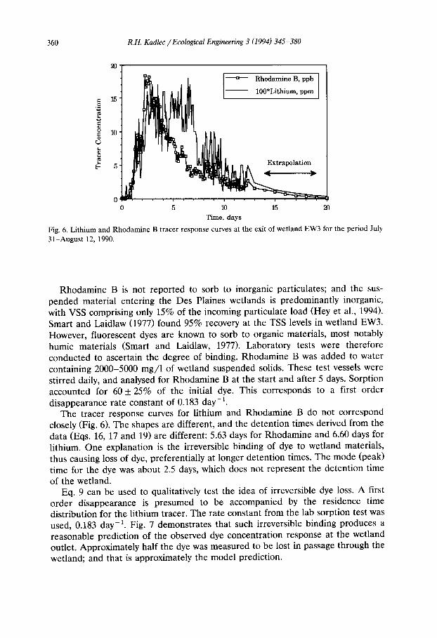
Fig. 6. Lithium and Rhodamine B tracer response curves at thc exit of wetland EW3 for the period July 31 -Augus t 12, 1990.

Rhodamine B is not reported to sorb to inorganic particulates; and the suspended material entering the Des Plaines wetlands is predominantly inorganic, with VSS comprising only 15% of the incoming particulate load (Hey et al., 1994). Smart and Laidlaw (1977) found 95% recovery at the TSS levels in wetland EW3. However, fluorescent dyes are known to sorb to organic materials, most notably humic materials (Smart and Laidlaw, 1977). Laboratory tests were therefore conducted to ascertain the degree of binding. Rhodamine B was added to water containing 2000-5000 mg/l of wetland suspended solids. These test vessels were stirred daily, and analysed for Rhodamine B at the start and after 5 days. Sorption accounted for 60 _+ 25% of the initial dye. This corresponds to a first order disappearance rate constant of 0.183 day-l.

The tracer response curves for lithium and Rhodamine B do not correspond closely (Fig. 6). The shapes are different, and the detention times derived from the data (Eqs. 16, 17 and 19) are different: 5.63 days for Rhodamine and 6.60 days for lithium. One explanation is the irreversible binding of dye to wetland materials, thus causing loss of dye, preferentially at longer detention times. The mode (peak) time for the dye was about 2.5 days, which does not represent the detention time of the wetland.

Eq. 9 can be used to qualitatively test the idea of irreversible dye loss. A first order disappearance is presumed to be accompanied by the residence time distribution for the lithium tracer. The rate constant from the lab sorption test was used, 0.183 day -1. Fig. 7 demonstrates that such irreversible binding produces a reasonable prediction of the observed dye concentration response at the wetland outlet. Approximately half the dye was measured to be lost in passage through the wetland; and that is approximately the model prediction.


3.3. Modeling

Three models are explored here that can explain the experimental tracer response curves: plug flow accompanied by dispersive mixing, well-mixed "tanks" (CSTRs) in series, and a series-parallel network of CSTRs.

Plug flow with dispersion In this model, mixing is presumed to follow a diffusion equation. It can be

shown that the same equation also describes the mixing which occurs due to a velocity profile in the direction transverse to flow (Fogler, 1992). A one-dimensional spatial model is chosen, for two reasons. First, analytical expressions are available for computation of pollutant removal for the one-dimensional case (see e.g., Fogler, 1992). Second, a two-dimensional version requires the two-dimensional velocity field, which is obtainable only with extreme difficulty. The tracer mass balance equation is a partial differential equation, which includes both spatial and temporal variability:

~2 C ~( uC ) aC (23)

D ~x 2 0x at '

where u = velocity, m/day ; D = dispersion constant, mm2/day; x = distance from inlet toward outlet, m.

The boundary conditions most appropriate for this mass balance are known as the closed-closed boundary conditions (Fogler, 1992). These imply that no tracer can diffuse back into the inlet pipe, nor back up the exit flume at the wetland outlet. Solutions to this mass balance have been available for more than two decades (Levenspiel, 1972). Only the pertinent results from those solutions are presented here.

0.09 ~ ^ ^ " [ - - -o-- - Sorption Model Smoothed I

.~ ~ o.t~ ~ [ ~ .3715°Dy e [ ~ ~ i -~ ~ 0.07

0.05 -

0.04

E "--.", 0 1 2 3 4 5 6 7 8 9 1{3 11 12

Time, days

Fig. 7. Rhodamine B tracer response curve and a first order sorption model for wetland EW3 for the period July 31-August 12, 1990. The dye concentrations have been scaled to match the modal concentration.


o

,.m

8

1.4

1.3 ! Model, D/uL = 0.2 I 1.2 - ----a-- August 91, D/uL = 0.13 ] Ii ' 0 • i I I ~ August 9,DIuL=0.231 1.0" 0.9 - 0.8 " 0.7 " 0.6 -" 0.5 : 0.4 i 0.3- 0.2 -' 01" o:o:

0•0 0.5 1.0 1.5 2.0 2.5

Number of Residence Times

Fig. 8. Plug flow plus dispersion model fit for the lithium tracer tests of August 1990 and August 1991. The less frequent sampling of 1991 shows a smoother curve.

The dimensionless pa ramete r which characterizes Eq. 23 is the Peclet number , or its inverse, the wetland dispersion number :

uL 1 Pe D . ~ ' (24)

where Pe = Peclet number , dimensionless; _~; = wetland dispersion number, dimensionless; L = distance from inlet to outlet, m. The two results of interest for the pulse test are the t racer detent ion time and the dimensionless variance:

"r = L / u , (25)

(7.2 2 2 r - - f = o.~ Pe Pe 2 ( 1 - e - P c ) ' (26)

where o .2 = dimensionless variance of t racer response. The wetland dispersion number may therefore be calculated f rom the moments of the t racer response curve (Eqs. 16, 19, 20, 22 and 26). Values of ~ ; range from 0.13 to 0.46 (Table 4).

It is also instructive to compare the predic ted shape of the t racer response curve to the observed data (Fig. 8). The model calculation for .~; = 0.2 (Levenspiel, 1972) is seen to be a reasonable approximation of the two August test results, for which the best fit values were 2 ; = 0.23 and 0.13, respectively. The mode of the model curve is located at about 60% of one mean detent ion time.

It should be noted that the solution of the partial differential Eq. 23 requires special numerical methods.

Tanks in series

A second method of introducing dispersion into the flow field is to conceptually section the wet land into a series of equal-sized, well-mixed regions. This model has also been in existence for over two decades (Levenspiel, 1972). This concept has


the effect of discretizing the spatial variation, and results in ordinary differential equations for the concentrations of the tracer in each of the well-mixed regions. This model contains two parameters, the mean detention time and the number of regions. The mathematics of the model are well established (Fogler, 1992), and only the necessary features are given here. The two results of interest for the pulse test are the detention time and the variance:

nV/ r = Q , (27)

0 -2 1 . . . . , ( 2 8 ) ,/.2 0-2 n

where V~ -- volume of the ith section, m3; n = number of sections. The number of sections may therefore be calculated from the moments of the tracer response curve (Eqs. 16, 19, 20, 22 and 28). Values of n range from 1.8 to 4.4, with an average of 2.7 (Table 4).

The model permits the calculation of the mode of the response curve; it is:

tp 1 0 o = - - 1 , (29)

~- n

where Or, = peak t ime/de ten t ion time; tp = peak time, day. Thus, the time for the peak to emerge is predicted to be between 45% and 77% of the detention time, according to this model (Table 3). Experimentally, this range was from 23% to 68%.

It is again instructive to compare the predicted shape of the tracer response curve to the observed data. The model calculation for the August 1991 test

1.0

0.9 ~ P ~ \ [ . . . . . 3 CSTRs

0s ° I " - ' , A \ I 4cs ,~/ \ % \ I . . . . . . . . . 5 CSTRs

0.7 ~ X ~ I ° August 91 I

i . ~ 0.1

0.0 ~ ° - - ~ - - - - 0.0 0.5 1.0 1.5 2.0 2.5 3.0

Number of Detention Times

Fig. 9. Well-mixed sections in series model compared to August 1991 data.


indicates 4.4 sections; Fig. 9 shows that to be a reasonable fit over the entire response. However, the number of sections may also be calculated by other curve fitting procedures, such as minimization of the mean square error between experimental points and the model. When this procedure is applied to the August 1991 data set, the value of n = 3.8, compared to 4.4 from the moment analysis.

Network model Not all the tracer response curves displayed the shape expected of either tanks

in series or a plug flow with dispersion models. Some tracer typically exited too early (bypassing), some was retained too long (storage). The simplest model which can produce these effects is a series of well-mixed zones in a main flow path, which interchange water and tracer with side zones that are not in the main flow path. Such a network was proposed by Levenspiel (1972) for chemical reactors; but the same notions were advanced by Valentine and Wood (1977) for river systems. More recently, Seo (1990) showed that a storage zone model was superior for describing pool and riffle flows.

The alternative network consists of a series of stirred sections, each of which is connected to a side section. The side sections represent areas out of the main flow path. These storage zones are modeled as CSTRs which exchange fluid elements with the main CSTRs via interchange flows. Levenspiel (1972) advances a version of this model which contains three parameters: the fraction of dead zones, the exchange rate, and the number of stages. This model has been adopted here as a potential improvement over the preceding models.

The compartmental model used for Des Plaines EW3 is a slight modification of the model described by Levenspiel (1972). Based on the analysis of the preceding section, a series of three CSTRs are envisioned to describe the main deep flow channel of the kidney shaped EW3 (Fig. 1). Although the basin averages about 60 cm in depth, the central area is deeper with only submergent and floating-leaved vegetation, while the fringes are shallow and densely covered with cattail. The

Plug Flow

Fig. 10. Patterns of flow model layout. Well-mixed sections in series interchange water and dissolved substances with side zones. A plug flow component permits use of a lag time for first tracer appearance

at the outlet.


shallow side zones are not in the direct flow path. They are represented as storage zones by three sections added in parallel to each side of the main flow sections, and are envisioned to exchange water with the central sections via wind-driven, biota-driven, and gradient-driven flows. These interchange flows can exchange dissolved and suspended constituents with the water passing in the main flow path. A sketch of this model is shown below in Fig. 10. The shallow, vegetated zones to the two sides of main flow may be combined for purposes of calculation.

This model must satisfy the dynamic wetland water budget calculations. The volume of each wetland zones will thus change with time according to pumping events, evaporation, etc. The total area occupied by the sex stirred sections is:

6

A = E A i , (30) i=1

where A; = section area, m 2. To keep the model simple, the number of zone sizes was limited to two; the three main flow zones were assumed to be of equal size, and the three side zones were also kept to one size. Thus:

A I = A 3 = A 5 , and A 2 = A 4 = A 6 . (31)

The dead zone fraction (4)) was defined as the fraction of volume occupied by the side zones, which is taken proportional to area for constant mean depth:

4) = (A 2 + A 4 + A 6 ) / A . (32)

In addition, the side zones were assumed to experience equal interchange flows (~). These flows might occur, for instance, as a result of wind-driven surface water moving into a side zone, and being balanced by a return flow across the wetland bottom.

This model has two adjustable parameters: 4) and q~. However, in a practical sense, the flushable water volume of the wetland is generally not known. Thus this volume becomes a third parameter.

Sectional water balances Sectional water balances are needed to calculate all connecting flowrates. The

water level in the wetland is essentially flat. As a result, one of the model criteria is to maintain equal water levels, h(t), in each section. These equations begin with a mass balance on each of the sections:

dV i 7 dt = ~-,Qji + ( P - ET)Ai , (33)

j = 0

where V/= section volume, m3; Oji = net flow from section j to section i; j = 0 refers to inflow source (pump); j = 7 refers to outflow sink (flume). Also,

V~ =Aih ( t ) (34)


and the A i are nearly constant over the range of fluctuation. Therefore, the level pool constraints are:

d ~ dh dt =Ai-"~ ' i = 1, 2 . . . . . 6. (35)

The level change, dh/d t , is determined from the overall water mass balance, Eq. 11. Eqs. 33 and 35 can be solved algebraically for the unknown flowrates Qij at any time. Interchange flows do not appear in these mass balances, since they are equal and opposite.

Dynamic tracer mass balances The tracer mass balances consist of a component balance on each of the mixed

zones. The derivation of these equations is a bit more complex than the zonal mass balances just discussed. For a tracer pulse of concentration C i entering the first zone, the tracer mass balance on this zone is:

d(ViCi) 7 6 dt EQjiC~+ EqJji(Cj-Ci) , i = 1 , 2 , . . . , 6 , (36)

j--O j - -1

where

k = i

and

k=j

if Oji < 0,

if Oji > O.

The interflow array components ~tji a r e zero except for qJ21 = ~043 = I]/65 = if/. These six coupled differential equations were solved numerically with a fourth order Runge -Ku t t a routine.

A lag time correction The tracer response curves display a delay between time zero, when the lithium

is dumped, to the time at which lithium is first measured at the outlet. This is characteristic of a transport delay superimposed on the CSTR network, and accordingly a constant-volume plug flow zone, with a detention time matching the lag time, was added to the model to account for this delay. The volume was determined using the average pumping rate during the run.

Vpf = 0 q ' p f , (37)

where Vpf = volume of plug flow zone, m3; Zpf = detention time in plug flow zone, day. The balance of the wetland volume was divided among the CSTR sections. The inclusion of this transport delay adds a third parameter to the model, Zpf.

Parameter determination The plug flow detention time Zpf measured directly from the experimental

distributions. As previously noted, errors in the calculation of basin volumes or flow rates caused discrepancies between measured and nominal detention times.


0.40 ~ - _ _

0.35

0.30

~ 0.25

~ 0.20

0.15

0.10

0.05

0.00 0 5 10 15 20 25

Time, days Fig. 11. Patterns of flow model fit to data for October, 1990.

For example, the determination of the exact basin topology was hampered by a difficulty in defining the basin floor. Therefore, it was necessary to set the model mean residence time equal to the experimental mean residence time, by adjusting the wetland volume. The average wetland depth becomes a parameter in the model fitting procedure (Kadlec and Bastiaens, 1992).

The remaining two parameters are the dead zone fraction ¢ and the interchange volumetric flow rate @. Both affect the simulated value of the outlet

0.35

[ " Data July 1991 I "~.~ 0.250"30 f ~ ~ l ~ [ Model (Oct 90 Parameters) ]

~ 0.20

0.15 ' .

0.10

0.05 '

0 . 0 0 , ~ . • • - , . . . . , . . . . , . . . . , . . . . . . . . ,

0 5 10 15 20 25 30 Time, days

Fig. 12. Patterns of flow model, with October, 1990 parameters, compared to July, 1991 data.


Table 5 Comparison of network parameters

Run T actual ~" plug flow Dead zone Interchange Throughflow (day) zone fraction flow Q

(day) 4) ~ (m3/day) (m3/day)

Ratio interchange: throughflow

Oct-90 6.99 1.00 0.50 2210 1625 1.36 Jun-91 6.36 1.00 0.30 170 1585 0.11 Jul-91 7.35 0.92 0.35 340 1465 0.23 Aug-91 12.45 0.08 0.30 0 580 0.00

lithium concentration. The best fit was chosen to minimize the sum of the squared errors.

Fit of first data set The model effectively simulated the October 1990 tracer concentration distribu-

tion curve (Fig. 11). The model thus adequately describes the flow patterns in EW3 during the time period of the tracer test. The optimum set of parameters included a plug flow detention time of one day, a 50% dead zone fraction, an interchange flow rate of 2210 m3/day, which was 1.36 times the average throughfiow of 1625 m3/day. The tracer detention time for this run was 6.22 days.

The three 1991 tracer runs of June, July and August were simulated using the parameters from the October, 1990 tracer test. Good predictions were not ob- tained (see for example Fig. 12). The parameters for each run were then individu- ally fit (Table 5). These new parameters produced a good fit (see for example Fig. 13).

0.35

0.30

0.25

0.20

0.15

0.i0

0.05

0.00 0 5 10 15 20 25 30

Time, days

Fig. 13. Patterns of flow model, with July, 1991 parameters, compared to July, 1991 data.


\° _.] 24o 3,0 Z-"

SIX DAYS AFTER INJECTION ~._

(c)

~ A / ,3 7 ,7 7 ~

54 12

33 17

TEN DAYS AFTER INJECTION ~_

Fig. 14. Progression of the lithium pulse (/zg/l) through the wetland during August, 1990. The tracer detention time for the entire wetland was 6.60 days.

3.4. Internal tracer measurements

There is no clear advantage to any of the three models in terms of ability to fit the data (Figs. 8, 9, and 11). Internal wetland stations were sampled during the August 1990 test, and provide a potential basis for model discrimination. Daily grab samples were taken at 26 interior locations (Fig. 1). Lithium concentrations at these locations give an indication of the rate of progress of the lithium pulse through the wetland, and of the spreading of the pulse due to mixing processes. The sequence of lithium maps shown in Fig. 14 depict the movement of the tracer "cloud" through the wetland. One day after the tracer was added to the inlet flow in a single dose, high lithium concentrations (ca. 200-300 ppb) were found throughout more than half the wetland (Fig. 14a), and these were rather uniformly distributed. The nominal detention time for this run was 6 days; and therefore the tracer had moved much further than would be anticipated (ca. 1/6 of the way to


0.15 [] Cattail [] Non-cattail

0.10

0.05 <

II 0.00 . . . . . . . . . . . . . . . . . . . . . . . . . . . .

Site

Fig. 15. Average tracer concentration at various interior wetland stations during the August , 1990 test, grouped by cover type. Cattail (Typha spp.) is not different from non-cattail (a = 0.05).

the outlet) if water moved in plug flow. Mechanisms that could contribute to such a tracer pattern include wind-driven mixing and velocity profile effects. Attempts at measuring local velocity profiles all failed because no measurement technique was found to determine the extremely low velocities involved (ca. 0.05 cm/s) .

After six days, the highest lithium concentrations (ca. 150 ppb) were found in the exit region of the wetland (Fig. 14b). However, lithium remained at lower concentrations (50-90 ppb) over much of the wetland, including the inlet region. After ten days, most of the tracer had been flushed from the wetland (Fig. 14c).

Tracer responses were not correlated with wetland characteristics at the sampling locations. Several such characteristics might affect tracer response: water depth, vegetation density, and distance from the shortest path through the wetland. In the test of August 1990, no such effects were found. The average tracer concentration over the period of sampling at each location is representative of the amount of tracer reaching that location. For instance, if a tracer did not reach a particular station, its concentration would average zero there. If the entire wetland were well-mixed, tracer would average the same value at all stations.

Average tracer concentrations were not significantly correlated (a = 0.05) with the presence of dense emergent vegetation, namely cattail (Fig. 2). Fig. 15 displays the averages for all stations; cattail clearly does not group apart from other stations. Average tracer concentrations were not significantly correlated (a = 0.05) with the water depth at the station (Fig. 1). Fig. 16 displays the averages for all stations ordinated by depth category; there is not a trend. Average tracer concentrations were not significantly correlated (a = 0.05) with the distance of the station from the main flow path (Fig. 1). Fig. 17 displays the averages for all stations ordinated by this distance category; there is not a trend.


Depth Range, cm =

8

II I]1 [[I IIIII i01110 Ill °11 0 . 0 0 . . . . . . . . . . . . . . . . . . . . . . . . . . . .

Site Fig. 16. Average tracer concentration at various interior wetland stations during the August , 1990 test, grouped by water depth. Various depths are not different (a = 0.05).

Neither the plug flow plus dispersion model nor the tanks in series model is strongly supported by these internal tracer measurements. The problem is too much mixing in the inlet half of the wetland. Fig. 18 shows the response curves averaged over the three consecutive thirds of the wetland, as well as the model response for those same sections. Section 1 contained 9 sample stations, section 2

Distance off main flow path, meters =

o.1~.1 ~1~ 1~ ~ ~

0 . ~ . . . . . . . . . . . . . . . . . . . . . . . . . . . .

Site

Fig. 17. Average tracer concentration at various interior wetland stations during the August , 1990 test, grouped by distance from presumed main flow path. Various distances are not different (a = 0.05).


0.30 ~ - ~

" CSTR #1 0.251 \ ~ csTR ~2

i 0.20

0.15

0.10

0.05

0.00 0 1 2 3 4 5 6 7 8 9 10 11 12

Time, days

0.30 " CSTR 1

"" '¢ ' - -- CSTR 2 0.25

CSTR 3

0.20

0.15

0.10

0.05

0.00 , • , . , • , . , • , • , • , • , • , • ,

0 1 2 3 4 5 6 7 8 9 10 11 12

Time, days

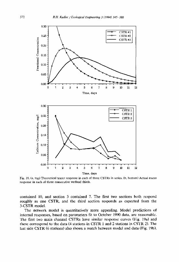
Fig. 18. (a, top) Theoretical tracer response in each of three CSTRs in series. (b, bottom) Actual tracer response in each of three consecutive wetland thirds.

contained 10, and section 3 contained 7. The first two sections both respond roughly as one CSTR, and the third section responds as expected from the 3-CSTR model.

The network model is quantitatively more appealing. Model predictions of internal responses, based on parameters fit to October 1990 data, are reasonable. The first two main channel CSTRs have similar response curves (Fig. 19a) and these correspond to the data (4 stations in CSTR 1 and 2 stations in CSTR 2). The last side CSTR (6 stations) also shows a match between model and data (Fig. 19b).

R.14. Kadlec / Ecological Engineering 3 (1994) 345-380 373

3.5. Comparison to ponds and rivers

Comparison to literature studies in more aquatic environments is possible. Most sources report a dimensionless dispersion number based on depth of the water body, D / u h , rather than length as for the wetland dispersion number D / u L . Table 6 summarizes mixing parameters calculated from several published sources.

Rivers Longitudinal mixing in rivers has been thoroughly investigated and reported

over the past three decades (Fischer et al., 1979; also summarized in French, 1985).

0.4

0.3'

0 .2

0.1'

0.0 0

----t--- Data Zone 1 d Model Zone 1

a l i l - : • a • l - l

2 3 4 5 6 7 8 9 10 Time, days

r.)

0.20

0.15 I --- t--- Data Zone6 I

Model Zone 6

• J " , ° , . .

! "',, ,';' " ' " ' t .............. o... 0"10

0.05

0.00 - - , - , • , - , - , • , - , - , • ,

0 1 2 3 4 5 6 7 8 9 10 Time, days

Fig. 19. Tracer response (a, top) in the inlet CSTR zone, and (b, bottom) in the last side CSTR zone, compared to network model. August 1990 data; October 1990 parameters.


Table 6 Mixing parameter values for wetland and aquatic systems

System Source Normalized System Depth variance dispersion dispersion or02 number number

D / u L D / u h

Wetlands Wetland EW3 Benton, KY Listowel, Ont. Richmond, N.S.W. Everglades

Ponds Nssuka, Nigeria Dredge Ponds

Rivers 22 Rivers & Channels 5 Rivers Experimental Channel

This study 0.40 + 0.10 0.26 + 0.10 89 + 34 TVA (1990) 0.22 0.12 136 Hershkowitz (1986) 0.13 0.07 117 Fisher (1990) 0.26 0.15 30 Rosendahl (1981) 0.14 0.07 50

Agunwamba (1992) 0.265 _+ 0.035 0.157 _+ 0.025 65 + 10 Thackson (1987) 0.40 _+ 0.28 0.48 -+ 0.64 77 _+ 38

Fischer et al. (1979) 60 +_ 41 Day (1975) 0.019-0.076 0.009-0.038 58 + 30 Seo (1990) 0.31 +0.05 0.19,+0.04

A summary of measurements for 22 rivers and channels of depth less than 1.1 m (Fischer et al., 1979) gave D/uh = 60 + 41, range: 12 to 160; where h = depth of the river, m.

Fischer et al. (1994) recommend estimation of dispersion according to:

u-h = 0.011 , (38)

where u * = shear velocity, m/day ; W = pond width, m. The shear velocity is in turn calculated from the slope of the channel and the hydraulic radius of the channel. In the present context, the large width of the wetland means that hydraulic radius is essentially equal to depth.

u * = /ghS , (39)

where S = river bed slope, m / m ; g = gravitational acceleration, m / d a y 2. In the wetland context, the problem becomes the estimation of this shear velocity. It is derived in the river context by presuming a velocity profile in the vertical direction, e.g., logarithmic. It may also be estimated from a description of fluid friction, which is frequently taken to be described by Manning's equation (French, 1985):

1 U = - - h 2/3 ~/S, (40)

n

where n = Manning's coefficient, s / m 1/3. Eqs. 39 and 40 combine to relate the shear velocity to Manning's coefficient. In fact,

u 1 - - = - - h - 1 / 6 ~ / g . (41) /A* g/


Values of Manning's coefficient are available from a few studies of wetland water flow (Rosendahl, 1981; Shih and Rahi, 1982; Kadlec, 1990). This coefficient takes on values of about 0.02-0.05 for streams and rivers; but is much larger for vegetated or partly vegetated wetlands, in the range of 0.3-3.0 s /m 1/3. The width to depth ratio for EW3 is 190. Presuming the lower value of Manning's coefficient of 0.3 s /m 1/3, Eqs. 38 and 41 produce a value of D/uh = 388 for EW3; the upper value n = 3.0 produces D/uh = 39. This range brackets the measured values. However, these estimates rely heavily on the estimate of Manning's coefficient.

Day (1975) tested several reaches of streams in New Zealand. His data show a smaller amount of mixing than found in EW3. In terms of dimensionless pulse variance, Day found values of tr 2 in the range 0.019 to 0.076, which correspond to values of D/uh = 5 to 20. Table 4 shows values for EW3 from 0.227 to 0.545. Day found more dispersion at lower flow rates, but all velocities were two orders of magnitude higher than in EW3. Day speculated that trapping might be important at lower velocities.

Valentine and Wood (1977) performed model calculations which suggested that "trapping" zones (recirculation eddies) greatly increased dispersion. Seo (1990) performed laboratory experiments on a pilot scale channel (50 m long by 2 m wide) which confirmed that a pool and riffle configuration indeed experienced more than "Fickian" dispersion. Seo's experiments produced values of 0, 2 in the range 0.26 to 0.36, which are in the middle of the range measured for EW3 (Table 6). It should be noted that river calculations are subject to open-open boundary conditions (Fogler, 1992), and consequently the system dispersion number is given by:

2 ~r2 = ~e" (42)

Ponds Ponds are perhaps a better analog to the wetland situation than rivers. Veloci-

ties in wastewater treatment lagoons are some tens of meters per day, which matches wetland velocities. Shallow ponds are in fact just the unvegetated extreme of a wetland.

Agunwamba et al. (1992) provide a summary analysis of recent mixing studies in waste stabilization ponds. They recommend an expression of the form:

h D ( u )0.82(W) -(°98+ 1385~ )

uh = 0.102 ~ - T (43)

They made measurements of dispersion in an unvegetated pond 0.3 m deep, 123 m long and 27 m wide in Nigeria, which gave D/uh = 64.5 + 10.3, N = 12, range: 45 to 88. Velocities in the pond were comparable to velocities in EW3. Eq. 43 correlated their data well (R 2 = 0.883, N = 12). When applied to wetland EW3, with W/h = 190 and n = 0.3, Eq. 44 gives D/uh = 37. Increasing n to 3.0 reduces D/uh to 3.7. These estimates are lower than the data in Table 4.


Agunwamba et al. (1992) also summarize data from three other studies, which were correlated by:

u~- = 0.119 , N = 4 7 . (44)

When applied to wetland EW3, with W / h = I90 and n = 0.3, Eq. 44 gives D / u h = 463. Increasing n to 3.0 reduces D / u h to 46. Again, this range brackets the measured values. Again these estimates rely heavily on the estimates of Manning's coefficient.

Thackson et al. (1987) investigated data from several dredged material contain- ment areas. Five of these had depths less than 1 m, and had aspect ratios (length to width ratios) in the range 1.6 to 3.2, which bracket that for EW3 (1.8). Several results from this study carry over to the wetland situation. First, the ratio of actual detention time to theoretical detention time for these ponds ranged from 19 to 63%, which is even less than the average of 67% measured for EW3 (Table 3). Second, the ratio of peak time to mean detention time was 0.46 + 0.25, compared to 0.49 + 0.33 for wetland EW3. Third, the range of ~ was from 0.08 to 0.82, which spans that found for EW3 (Table 4).

3.6. Comparison to other wetlands

There are other reports of wetland tracer studies (see e.g., Fisher, 1990; Cooper, 1992; Egger, 1992; Pilgrim et al., 1992). However, most of these do not involve any attempt to quantify the effects of mixing via flow modeling. Table 6 summarizes calculations made for several wetland systems. Care must be exercised in interpretation of the data in Table 6; all studies listed except EW3 were done with fluorescent dyes, and are therefore subject to sorption errors.

TVA (1990) performed Rhodamine WT tracer studies at a free water surface wetland in Benton, KY. That tracer response showed a peak time equal to 67% of the mean tracer detention time. The tracer detention time was 80-98% of the nominal detention time, depending on the assumption made for wetland water volume. Kadlec et al. (1993) illustrated that the tracer response was characterizable by the volume being apportioned 40% to a PFR, 30% to CSTR 1 and 30% to CSTR 2. However, the dimensionless variance shown in Table 6 (0.22) would also be produced by four to five CSTRs in series (n = 4.6).

Dye tests at Listowel, Ontario (Hershkowitz, 1986) indicated internal peak times that were about 40% of the nominal detention time. Kadlec et al. (1993) estimated that the tracer response was characterizable by about four CSTRs in series.

Fisher's (1990) data indicate a peak time which is 55% of the tracer detention time. Kadlec et al. (1993) illustrated that the tracer response was characterizable by the volume being apportioned 34% to a PFR, 33% to CSTR 1 and 33% to CSTR 2. However, the dimensionless variance shown in Table 6 (0.26) would also be produced by four CSTRs in series (n = 3.9).

Rosendahl (1981) correlated both velocity and the dispersion constant as a function of depth in Shark River Slough, an Everglades freshwater marsh. The


marsh dispersion number was found to be D / u L = 0.068 + 0.002 for depths in the range of 12 to 91 cm. However, this value is somewhat in error, since the detention time was taken to be the peak time; which yields velocities that are too high.

There is a surprisingly narrow range of depth dispersion numbers which characterize wetlands, shallow rivers and shallow ponds (Table 6). Aspect ratios ( L / W ) for river studies tended to be high, ca. 1000:1, and therefore system dispersion numbers were low compared to those for ponds and wetlands, which typically have aspect ratios in the range of 1 : 1 to 25 : 1.

4. Conclusions

The network model did the best job of describing the Des Plaines EW3 tracer response curves. However, both tanks in series and dispersion models adequately simulated the exit responses.

Parameter estimation includes determination of the detention time of the wetland. The Des Plaines experimental wetlands were constructed and surveyed with more than normal care, yet the water volumes were not known with sufficient accuracy. Likewise, both inflows and outflows were measured and cross checked with redundant metering, more than the normal effort. Yet outlet water flows were not measured with sufficient accuracy. Consequently, the calculation of nominal detention time produced a value which was in error by as much as 50% (high). Models of wetland water chemistry involve the concept of contact time, and it seems necessary to quantify it more accurately than by use of a nominal detention time.

Tracer detention time is the most logical candidate, since it forces closure of the mass balance for a non-reactive dissolved constituent. However, it must be noted that closure of the tracer mass balance is prerequisite to a good tracer test. Detent ion time is a necessary ingredient in all mass balance models currently in use.

The use of peak travel time as a surrogate for tracer detention time is appealing, since there is no need to measure volumes or flows, nor to measure a complete response curve. Unfortunately, all data and all models lead to the same conclusion: peak times are much shorter than tracer detention times, often by a factor of two. Use of a sorbing tracer can further compound this error, since sorption shortens the peak time still further.

The data from all wetland, river and pond studies indicate that the degree of mixing of waters in passage through the system is not small. One measure of the degree of mixing might be taken as the dimensionless variance of a pulse tracer test ~ro 2. This paramete r is zero for a plug flow system, and unity for a totally mixed system. Thus the wetlands and shallow ponds in Table 6 are from 13 to 40% of the way from plug flow to completely mixed.

The information contained in an R T D may be used in Eq. 10 to calculate the conversion of a pollutant. The difference between exit concentrations for plug flow


and completely mixed wetlands of the same detention time can be large for efficient systems (Kadlec et al., 1993).

There is another useful fact about ~ro2: it is a close approximation to the fraction of the way between PFR exit concentration and CSTR exit concentration for a system conducting a volumetric first order reaction of a dissolved constituent, regardless of the size of the rate constant. To illustrate, suppose that a PFR of a given detention time converts 95% of a pollutant, leaving 5%. A CSTR of the same detention time would leave 25% of the pollutant. A partially mixed wetland of the same detention time, with cr d = 0.5 would leave 15% unconverted (14.2% with no approximation). Thus ~r 2 represents an approximate linear interpolator between concentrations remaining in the PFR and the CSTR for a volumetric first order reaction.

Obviously, not all reactions will be first order volumetric, in the wetland context. Other volumetric reactions may be calculated using the E-function and the appropriate kinetic rate expression, as indicated in Eq. 10.

Many wetland reactions are believed to involve sediments or biota that are distributed on an areal basis. To calculate constituent concentrations in this situation, it is necessary to know where the water spends its time in passage through the wetland. A network model can provide this information, whether it be CSTRs in series, or the more complex network which described EW3. For EW3, the network model required tracer detention time ~- and three other parameters: a PFR lag time, ~'pf, a dead zone fraction ~b, and an exchange flow ~b. Calculations for any spatially non-uniform wetland conducting areal reactions will require a model of this complexity.

Dynamics do not appear to influence the tracer behavior of EW3 to any marked extent, as illustrated by the success of the use of time average flow rates. Further, effects of pumping dynamics at Des Plaines are not predicted to have a significant effect on chemical reaction processes; these may also be treated on an average basis. This topic is explored in more detail in Kadlec and Bastiaens (1992). However, it should be noted that the pumping time periods for EW3 (once per day) were shorter than the detention times (6-12 days). Similar conclusions likely do not hold for event frequencies which are comparable or slower than the turnover frequency (detention time).

Dynamics do influence the observed degree of mixing. Each pumping event moved ten centimeters of water to all areas of the wetland, and each weekend moved fifteen centimeters of water to all areas. Thus the shallow areas were turned over several times during a 3-week test and these areas contained the densest emergent macrophytes.

Acknowledgements

Lithium and dye analyses were performed by Dave Wochaski in 1990, and Shelly Rivette in 1991. Dave Urban (1990) and Barbie Ballack (1991) performed on-site sample collection. Willem Bastiaens did the network model calculations.

R.H. Kadlec / Ecological Engineering 3 (1994)345-380

Financial support was provided by the U.S. Environmental through Wetlands Research, Inc.

379

Polution Agency

References

Agunwamba, J.C., N. Egbunniwe and J.O. Ademiluyi, 1992. Prediction of the dispersion number in waste stabilization ponds. Water Res., 26: 85-89.

Call, M.L., 1989. Estimation of micromixing parameters from tracer concentration fluctuation measurements. PhD Thesis, The University of Michigan, Ann Arbor, MI, 356 pp.

Cooper, A.B., 1992. Coupling wetland treatment to land treatment: an innovative method for nitrogen stripping. In: Wetland Systems in Water Pollution Control. IAWQ, Sydney, Australia, pp. 37.1-37.9.

Curl, R.L. and M.C. McMillan, 1966. Accuracy in residence time measurements. AIChE J., 12: 819-822.

Danckwerts, P.V., 1953. Continuous flow systems: distribution of residence times. Chem. Eng. Sci., 2: 1-13.

Day, T.J., 1975. Longitudinal dispersion in natural channels. Water Resour. Res., 11: 909-918. Egger, P., 1992. Wetland treatment for trace metal removal from mine drainage: the importance of

aerobic and anaerobic processes. In: Wetland Systems in Water Pollution Control. IAWQ, Sydney, Australia, pp. 46.1-46.9.

Fennessey, M.S., J.K. Cronk and W.J. Mitsch, 1994. Macrophyte productivity and community development in created freshwater wetlands under experimental hydrological conditions. Ecol. Eng., 3: 469-484.

Fischer, H.B., E.J. List, R.C.Y. Koh, J. Imberger and N.H. Brooks, 1979. Mixing in Inland and Coastal Waters. Academic Press, New York, 483 pp.

Fisher, P.J., 1990. Hydraulic characteristics of constructed wetlands at Richmond, NSW, Australia. In: P.F. Cooper and B.C. Findlater (Eds.), Constructed Wetlands in Water Pollution Control. Perga- mon Press, Oxford, pp. 21-32.

Fogler, H.S., 1992. Elements of Chemical Reaction Engineering, Second Edition. Prentice-Hall, Englewood Cliffs, NJ, 838 pp.

French, R.H., 1985. Open-Channel Hydraulics. McGraw-Hill, New York, NY, 705 pp. Hershkowitz, J., 1986. Listowel Artificial Marsh Project Report. Ontario Ministry of the Environment,

Water Resources Branch, Toronto, 251 pp. Hey, D.L., K.R. Barrett and C. Biegen, 1994. The hydrology of four experimental constructed marshes.

Ecol. Eng., 3: 319-343. Kadlec, R.H., 1990. Overland flow in wetlands: vegetation resistance. ASCE J. Hydraul. Eng., 116:

691-706. Kadlec, R.H. and W.V. Bastiaens, 1992. The use of residence time distributions (RTDs) in wetland

systems. Chapter 2, Volume II of The Des Plaines River Wetlands Demonstration Project, Report to USEPA, July 1992, 74 pp.

Kadlec, R.H., W. Bastiaens and D.T. Urban, 1993. Hydrological design of free water surface treatment wetlands. In: G.A. Moshiri (Ed.), Constructed Wetlands for Water Quality Improvement. Lewis Publishers, Boca Raton, FL, pp. 77-86.

Levenspiel, O., 1972. Chemical Reaction Engineering, Second Edition. John Wiley & Sons, New York, NY, 578 pp.

Mitsch, W.J. and J.G. Gosselink, 1993. Wetlands, Second Edition. Van Nostrand Reinhold, New York, NY, 641 pp.

Netter, R. and W. Bischofsberger, 1990. Hydraulic investigations on planted soil filters. In: P.F. Cooper and B.C. Findlater (Eds.), Constructed Wetlands in Water Pollution Control. Pergamon Press, Oxford, pp. 11-20.

Pauly, U., A. Horstmeyer and A. Odenthal, 1990. Integration von Abwasser- und Schlammbehandlung im Wurzelraumverfahren. Berichte zur t~kotechnik, Gesamthochschule Universitat Kassel, Ger- many, pp. 60-74.


Perry, R.H. and C.H. Chilton, 1973. Chemical Engineers' Handbook, Fifth Edition. McGraw-Hill, New York, NY.

Pilgrim, D.H., T.J. Schulz and I.D. Pilgrim, 1992. Tracer investigation of the flow patterns in two field-scale constructed wetland units with subsurface flow. In: Wetland Systems in Water Pollution Control. IAWQ, Sydney, Australia, pp. 19.1-19.9.

Reddy, K.R. and E.M. D'Angelo, 1994. Soil processes regulating water quality in wetlands. In: W.J. Mitsch (Ed.), Global Wetlands: Old World and New. Elsevier, Amsterdam, pp. 309-324.

Rosendahl, P.C., 1981. The determination of Manning's roughness and longitudinal dispersion coeffi- cients in the Everglades marsh. Paper presented at the Symposium on Progress in Wetlands Utilization and Management, Orlando, FL, June 1981, 22 pp.

Seo, I.W., 1990. Laboratory and numerical investigation of longitudinal dispersion in open channels. Water Resour. Bull., 26: 811-822.

Shih, S.F. and G.S. Rahi, 1982. Seasonal variations of Manning's roughness coefficient in a subtropical marsh. Trans. ASAE, 25: 116-120.

Smart, P.L. and I.M.S. Laidlaw, 1977. An evaluation of some fluorescent dyes for water tracing. Water Resour. Res., 13: 15-33.

Tennessee Valley Authority, 1990. Unpublished dye study results from September, 1990 at Benton KY. Thackson, E.L., F.D. Shields Jr. and P.R. Schroeder, 1987. Residence time distributions of shallow

basins. J. Environ. Eng. ASCE, 113: 1319-1332. Urban, D.T., 1990. Methods of determining residence time distributions in a reconstructed wetland. MS

Thesis, Illinois Institute of Technology, Chicago, IL, 76 pp. Valentine, E.M. and I.A. Wood, 1977. Longitudinal dispersion with dead zones. J. Hydraul. Div. ASCE,

103: 975-990. Wetlands Research, Inc., 1992. The Des Plaines River Wetlands Demonstration Project. Report to

USEPA, July 1992, 7 Volumes, Wetlands Research, Inc. Chicago, IL.

Detention and mixing in free water wetlands

Documents

Transcript of Detention and mixing in free water wetlands