Draft: October 31, 2013

Detection of Potential Transit Signals in Sixteen Quarters of

Kepler Mission Data

Peter Tenenbaum, Jon M. Jenkins, Shawn Seader, Christopher J. Burke, Jessie L.

Christiansen1, Jason F. Rowe, Douglas A. Caldwell, Bruce D. Clarke, Jeffrey L. Coughlin,

Jie Li, Elisa V. Quintana, Jeffrey C. Smith, Susan E. Thompson, and Joseph D. Twicken

SETI Institute/NASA Ames Research Center, Moffett Field, CA 94305, USA

peter.tenenbaum@nasa.gov

Michael R. Haas, Christopher E. Henze, Roger C. Hunter, and Dwight T. Sanderfer

NASA Ames Research Center, Moffett Field, CA 94305, USA

Jennifer R. Campbell, Forrest R. Girouard, Todd C. Klaus, Sean D. McCauliff, Christopher

K. Middour, Anima Sabale, Akm Kamal Uddin, and Bill Wohler

Orbital Sciences Corporation/NASA Ames Research Center, Moffett Field, CA 94305, USA

and

Thomas Barclay and Martin Still

BAER Institute/NASA Ames Research Center, Moffett Field, CA 94305, USA

ABSTRACT

We present the results of a search for potential transit signals in four years

of photometry data acquired by the Kepler Mission. The targets of the search

include 111,800 stars which were observed for the entire interval and 85,522 stars

which were observed for a subset of the interval. We observed that 9,743 targets

contained at least one signal consistent with the signature of a transiting planet,

where the criteria for detection are periodicity of the detected transits, adequate

signal-to-noise ratio, and acceptance by a number of tests which reject false

positive detections. When targets that had produced a signal were searched

repeatedly, an additional 6,542 signals were detected on 3,223 target stars, for a

total of 16,285 potential transiting planet signatures. Comparison of the set of

detected signals with a set of known and vetted transit events in the Kepler field

of view shows that the recovery rate for these signals is 97.0%. The ensemble

properties of the detected signals are reviewed.

– 2 –

Subject headings: planetary systems – planets and satellites: detection

1. Introduction

We have reported on the results of past searches of the Kepler Mission data for signals

of transiting planets, in particular the search of the first three quarters (Tenenbaum et al.

2012) and the search of the first three years (Tenenbaum et al. 2013). We now update and

extend those results to incorporate an additional year of data acquisition and an additional

year of Kepler Pipeline development.

1.1. Kepler Science Data

The details of Kepler operation and data acquisition have been reported elsewhere (Haas

et al. 2010). In brief: the Kepler spacecraft is in an Earth-trailing heliocentric orbit and

maintained a boresight pointing centered on α = 19h22m40s, δ = +44.5◦. The Kepler pho-

tometer acquired data on a 115 square degree region of the sky. The data were acquired

in 29.4 minute integrations, colloquially known as “long cadence” data. The spacecraft was

required to rotate about its boresight axis by 90 degrees every 93 days in order to keep

its solar panels and thermal radiator correctly oriented; the interval which corresponds to

a particular rotation state is known colloquially as a “quarter.” Because of the quarterly

rotation, target stars were observed throughout the year in 4 different locations on the focal

plane. Science acquisition was interrupted monthly for data downlink, quarterly for maneu-

ver to a new roll orientation (typically this is combined with a monthly downlink to limit

the loss of observation time), once every 3 days for reaction wheel desaturation (one long

cadence sample is sacrificed at each desaturation), and at irregular intervals due to space-

craft anomalies. In addition to these interruptions which were required for normal operation,

data acquisition was suspended for 11.3 days, from 19:39 Z 2013 January 17 through 03:50

Z 2013 January 29 (555 long cadence samples): during this time, the spacecraft reaction

wheels were commanded to halt motion in an effort to mitigate damage which was being

observed on Reaction Wheel 4, and spacecraft operation without use of reaction wheels is

not compatible with high-precision photometric data acquisition.

1Current affiliation: NASA Exoplanet Science Institute, California Institute of Technology, Pasadena,

CA 91125, USA

– 3 –

In July 2012, one of the four reaction wheels used to maintain spacecraft pointing during

science acquisition experienced a catastrophic failure. The mission was able to continue,

using the remaining three wheels to permit 3-axis control of the spacecraft, until May of

2013. At that time a second reaction wheel failed, which forced an end to Kepler data

acquisition in the nominal Kepler field of view. As a result, the analysis reported here is the

first which incorporates the full volume of data acquired from that field of view.

Kepler science data acquisition began at 00:00:00 UTC on 2009 May 12, and acquisition

of Quarter 16 data concluded at 11:17:11 UTC on 2013 April 8. This time interval contains

69,810 long cadence intervals. Of these, 4,726 were consumed by the interruptions listed

above, and 65,084 long cadence intervals were dedicated to science data acquisition. An

additional 1,076 long cadence intervals were excluded from use in Transiting Planet Search

(TPS) pipeline module. These samples were excluded due to data anomalies which came to

light during processing and inspection of the flight data. This includes a contiguous set of

255 long cadence samples acquired over the 5.2 days which immediately preceded the 11 day

downtime described above: the shortness of this dataset combined with the duration of the

subsequent gap led to a judgement that the data would not be useful for transiting planet

searches.

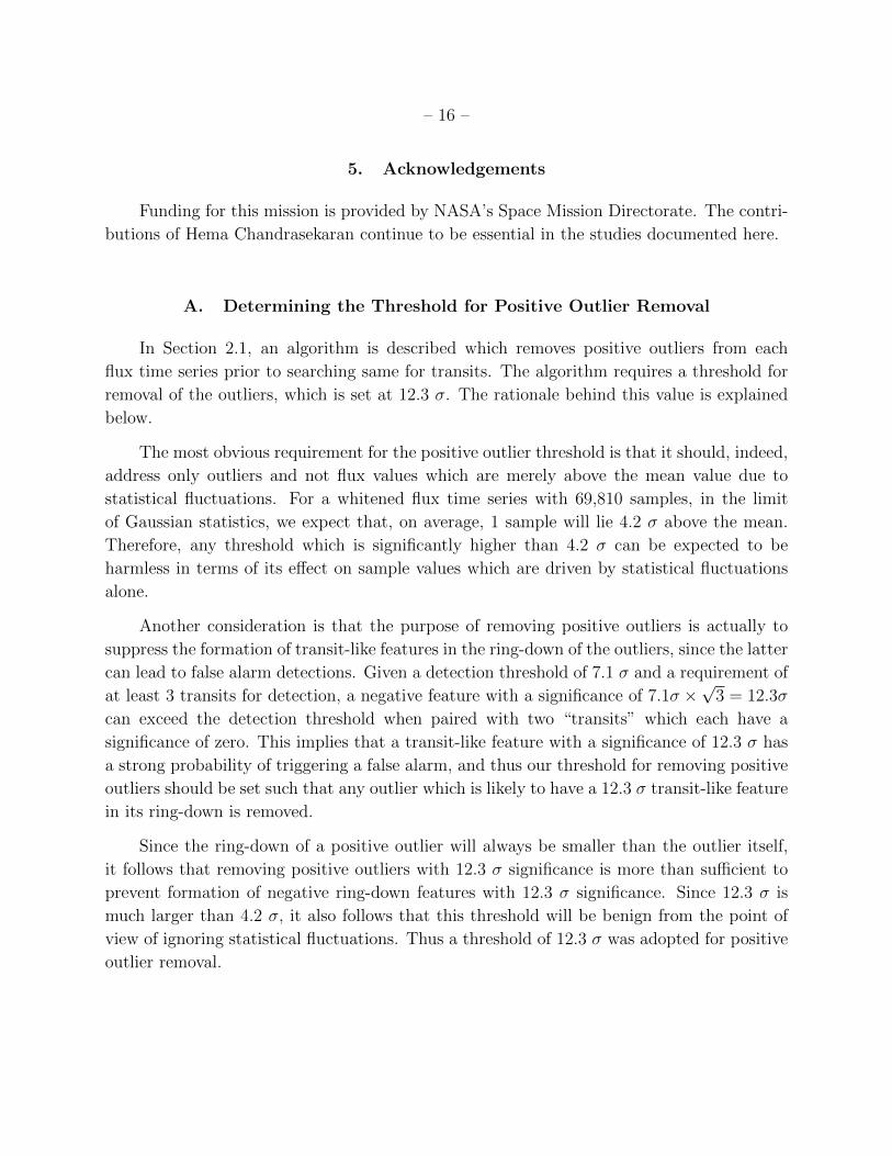
A total of 197,322 target stars were observed during some portion of Kepler’s four years

of data acquisition and were subsequently searched for evidence of transiting planets. Figure

1 shows the distribution of targets according to the number of quarters of observation. A

total of 111,800 targets were observed for all 16 quarters. An additional 39,964 targets were

observed for 13 quarters: the vast majority of these targets were in regions of the sky which

are observed in some quarters by CCD Module 3, which experienced a hardware failure in

its readout electronics during Quarter 4, resulting in a “blind spot” which rotates along with

the Kepler spacecraft. The balance of 45,558 targets which were observed for some other

number of quarters is largely due to gradual changes in the target selection process over the

duration of the mission.

As described in Tenenbaum et al. (2013), some eclipsing binaries are excluded from

TPS. In this case, a total of 1,519 eclipsing binaries were excluded. This number is smaller

than the number excluded in the Q1-Q12 analysis due to a change in exclusion criteria.

Specifically, we excluded eclipsing binaries from the most recent Kepler catalog of eclipsing

binaries (Kirk et al. 2013) that did not meet the criteria of being “transit-like”. Eclipsing

binaries were considered to be transit-like only if all of the following criteria were met:

1. The primary eclipse depth is greater than or equal to zero, i.e., flux must decrease at

primary eclipse

– 4 –

2. The primary and secondary eclipse depths are within 10% of each other OR the sec-

ondary eclipse depth is less than 10% of the primary eclipse depth

3. If detected, the phase of secondary eclipse has to occur within the range 0.49 - 0.51,

i.e., the binary star’s orbit must be near-circular

4. The morphology of the system, as defined in Kirk et al. (2013), has to be < 0.6, i.e.,

the primary and secondary eclipses must be well separated from one another.

Thus, the excluded eclipsing binaries are largely contact binaries which produce the most

severe misbehavior in TPS, while well-detached, transit-like eclipsing binaries are now pro-

cessed in TPS. This was done in order to ensure that no possible transit-like signature was

excluded, and also to produce examples of the outcome of processing such targets through

both TPS and Data Validation Wu et al. (2010); Twicken et al. (2014), such that quanti-

tative differences between planet and eclipsing binary detections could be determined and

exploited for rejecting other, as-yet-unknown eclipsing binaries detected by TPS.

1.2. Pre-Search Processing

Since the publication of Tenenbaum et al. (2013), there have been considerable im-

provements to the Pre-Search Data Conditioning (PDC) component of the Kepler pipeline.

The purpose of PDC is to remove variations in the flux time series which are generated by

changes in the spacecraft environment or other systematic effects. PDC performs very well

for the majority of targets in the Kepler Field of View. However, for an appreciable minority

the Bayesian Maximum A Posteriori (PDC-MAP) algorithm (Smith et al. 2012) does not

produce acceptable corrections of the visible systematics. To further minimize the number of

targets for which PDC-MAP fails to perform admirably a new method has been developed:

multi-scale MAP (or msMAP). Utilizing an overcomplete discrete wavelet transform the new

method divides each light curve into multiple channels, or bands, based upon characteristic

signal scales in time and frequency. This produces three time series for each flux time series:

one dominated by each of short-timescale, medium-timescale, and long-timescale variations.

The PDC-MAP algorithm is then applied to each band separately, which allows for a better

separation of characteristic signals and cleaner removal of the systematics. Relevant to tran-

sit detection, the new msMAP provides two distinct improvements to the PDC processed

data. The first is a significantly improved removal of thermal transients which occur in the

transition from Earth-pointing to science pointing after each data downlink. The second is

a modest reduction in introduced noise.

– 5 –

A second significant improvement to PDC is that it now “protects” known transits

from false detection as Sudden Pixel Sensitivity Dropouts (SPSDs) or other types of outlier.

Cadences containing known transits and eclipses are computed using the known epoch, period

and duration of the events. No SPSDs or outliers are flagged during the known transits.

This helps preserve transit depths and shapes from corruption by the SPSD and outlier

correction algorithms. Note that this only affects known transits. There is still the risk of

transit corruption for as yet undetected transits. However, once the transits are detected

and validated, subsequent data processing iterations will incorporate the new information.

2. Transiting Planet Search

This section describes the changes which have been made to the TPS algorithm since

Tenenbaum et al. (2013). For further information on the algorithm, see Jenkins (2002),

Jenkins et al. (2010b), and Tenenbaum et al. (2012).

2.1. Removal of Positive Flux Outliers

As described in Section 2.4 of Tenenbaum et al. (2013), removal of negative flux outliers

is a hazardous action, since it relies upon an algorithmic capability to distinguish between

a true outlier and a transit, and for obvious reasons removing the latter is frowned upon.

For this reason, strict limitations are placed upon the algorithm’s capabilities for removing

suspected negative outliers.

Positive outliers are much less risky to remove, since by definition a positive outlier

looks like the opposite of a transit. At first glance, one might therefore assume that positive

flux outliers are irrelevant as a source of false alarms or other difficulties, since the difference

between a short-duration positive flux excursion and a short-duration negative flux excur-

sion is intuitively obvious to the most casual observer. In actuality, however, positive flux

excursions can result in false alarm detections via the following mechanism: when a positive

flux excursion is subjected to the whitening filter, the whitened result includes ringing which

precedes and follows the excursion, as shown in Figure 2. The strongest components of the

ring-down have the opposite sign to the original excursion, thus a positive excursion in the

flux results in two negative excursions in the whitened flux, which are often misconstrued as

transits by the subsequent search.

The removal of positive outliers is accomplished by marking their locations in the

quarter-stitched flux time series as gaps and applying the standard TPS gap filling algo-

– 6 –

rithm. The identification of positive outliers, by contrast, makes use of the whitened flux.

The advantage to this is that by design the whitened flux contains only Gaussian-distributed,

zero mean, unit variance white noise, plus quasi-impulsive outliers; consequently, the posi-

tive outliers are extremely easy to identify in the whitened flux. The disadvantage is that

a positive outlier in the whitened flux can either indicate a positive outlier in the original

flux, or it can be part of the ring-down of a negative outlier such as a transit; this can be

visualized by inverting the lower plot in Figure 2. Thus the algorithm for positive outlier

removal is as follows:

• whiten the quarter-stitched flux

• identify clusters of whitened flux values which exceed a threshold: in this case a thresh-

old of 12.3 σ is used, as explained in Appendix A

• determine whether each cluster is due to positive outliers in the original flux or due

to the ring-down of negative outliers in the original flux: this is accomplished by

examining the local minima adjacent to each cluster, since for positive outliers the

local minima will be weaker than the positive outliers, whereas for the ring-down of a

transit one of the local minima will be much stronger than the positive outliers

• for each positive outlier value thus identified, mark the cadences in the quarter-stitched

flux as gapped and apply gap-filling

• produce a new whitened flux from the outlier-removed quarter-stitched flux and iterate

the process until no further positive outliers are identified: this takes account of the

fact that removal of outliers can change the local noise characteristics slightly, causing

values which had previously been below threshold to exceed the threshold.

2.2. Limitation on Allowable Transit Duty Cycles

An additional means of separating likely transiting planet signatures from false alarms

is to apply bounds to the ratio of the transit duration τ to the orbital period T . Equation

1 of Gilliland et al. (2000) shows the relationship between these parameters for Solar stellar

properties and a circular orbit:

τ [hours] = 1.4T [days]1/3. (1)

Equation 1 can be rewritten in terms of the transit duty cycle φdut ≡ τ/T :

φdut = 0.058T [days]−2/3. (2)

– 7 –

For late-type M dwarf stars, the constants in Equations 1 and 2 are 0.63 and 0.026, re-

spectively. A detection for which φdut is either much larger or much smaller than would

be expected from Equation 2 is unlikely to be actual transit signatures and as such can be

prevented from producing a TCE.

The shortest orbital period included in TPS searches is 0.5 days. At this limit, the

Solar-parameter value of φdut is approximately 0.092. To allow margin for elliptical orbits

or stars which are far from Solar in their parameters, we limit the maximum allowed value

of φdut to 0.16. This restriction is implemented by adjusting the minimum search period for

each trial transit duration used in the search: for 1.5 hour transits, the search is allowed to

operate down to periods of 0.5 days, while for 15 hour transits the minimum search period

is limited to 3.9 days. This restriction was also enforced in the Q1-Q12 processing reported

in Tenenbaum et al. (2013).

In the Q1-Q16 processing, an additional restriction was placed on the lower bound of

allowed φdut values, specifically

φdut ≥ 0.017T [days]−2/3. (3)

This limit is 3.4 times smaller than that expected for Solar stars and 1.5 times smaller

than expected for late M dwarf stars, which allows margin for elliptical orbits, large impact

parameter values, and non-Solar parameters. Equation 3 sets a maximum search period

which is a function of transit duration: for example, 1.5 hour transits are limited to search

periods of 50 days or less, while 3.0 hour transits are limited to search periods of 300 days

or less.

2.3. Detection and Vetoing of Potential Signals

Out of the 197,322 targets which were searched by TPS, a total of 112,981 were found

to have at least one periodic signal which exceeded the multiple event statistic of 7.1 σ, while

84,341 had no such signal. In this regard, current experience is consistent with past TPS

analyses, in which the number of targets for which the maximum multiple event statistic

exceeded the detection threshold was unphysically large, implying that the vast majority of

these events are false alarms. As in the past, a series of vetoes are used to eliminate false

alarms to the extent possible without rejecting excessive numbers of true transit signals.

The vetoes which are used in the current analysis – a robust statistic and a series of vetoes

based upon χ2 statistics – are described in modest detail in Tenenbaum et al. (2013), and in

particular the χ2 vetoes are described in considerable detail in Seader et al. (2013), so only

a description of changes to these quantities will be given here.

– 8 –

The multiple event statistic as well as the robust statistic only admit detections with

three or more transits. In detections where there are only three transits, the multiple event

statistic is blind to the quality of each transit whereas the robust statistic scrutinizes each of

the three transits to veto situations where one or more of the three transits overlaps signif-

icantly with a region of data that is anomalous in some way. The algorithm for examining

the transits for this case has changed slightly from that employed to produce the Q1-Q12

results in Tenenbaum et al. (2013). The past algorithm required that no more than 50%

of in-transit cadences be marked as anomalous for any of the three transits, whereas the

current algorithm requires that the average of the in-transit data quality weights be at least

0.5. Making this slight change has exposed an undesired sensitivity in the robust statistic

algorithm. This change is responsible for an increase in long period false alarms which is

discussed in Section 3. Future development work will be directed at enabling the χ2 vetoes

to identify these long period false alarms by including the data quality weights in the calcula-

tion of the degrees of freedom of the statistic (which are ultimately used in the computation

of the reduced χ2).

The two versions of the χ2 vetoes described in Tenenbaum et al. (2013) are again em-

ployed to produce the results of this paper. The first of these, χ2(1), remains unchanged.

There are some subtle issues, however, associated with the construction of χ2(2) which are

discussed at length in Seader et al. (2013) but will be briefly mentioned here for complete-

ness. Correcting for these subtleties enhances the vetoing efficiency of χ2(2) by enabling both

the quantities it is computed from and the statistic itself to have the correct statistical prop-

erties as described in both Allen (2004) and Seader et al. (2013). The first subtlety is that

the χ2(2) calculation implicitly requires that the calculated noise properties of the flux time

series are not changed by the presence or absence of a transit signal. In fact, while the noise

calculation is relatively robust against the effect of transits, it is not formally invulnerable:

while the presence or absence of a transit results in a change in the noise estimate which is

small enough to be neglected in the Multiple Event Statistic calculation, it was found to have

an effect on the value of χ2(2). This is addressed by applying the TPS auto-regressive gap-fill

algorithm to the cadences which are in-transit, which produces a flux time series which is

effectively transit-free; this time series is used to calculate the noise properties of the flux

time series for the purpose of χ2 discriminator calculations. The remaining subtleties arise

from the assumption that each transit is localized in time and isolated from every other

transit (i.e., the transit model consists of a series of short intervals of negative values sepa-

rated by longer intervals of zero values). While this is true for the unwhitened transit model,

it is not true for the whitened transit model, which is the model which must be used in

the calculation of the discriminators: in the whitened domain, the transits are “smeared,”

such that there are no cadences which have a model value of zero, and thus the value of

– 9 –

the model at one transit depends to greater or lesser extent on the values of all the other

transits. To mitigate thse effects, the χ2 contribution from each transit is calculated with all

other transits replaced by the auto-regressive gap fill values used for the noise calculation,

thus effectively performing the calculation for each transit as though it was the only transit

in the flux time series; in addition, the calculation neglects any cadence which is outside of

that transit, as determined by the unwhitened model, so that the effect of “smearing” into

out-of-transit cadence times is eliminated.

In addition to the above changes to existing vetoes, another version of the χ2 veto was

implemented that is more akin to a classical χ2 and is described in great detail in Seader et

al. (2013) as χ2(3). In this version, each single event statistic is compared with a calculated

expectation value in the whitened time domain (to avoid the subleties mentioned above).

These differences are then summed according to the exact expression for a classical χ2,

including division by the expectation value. The thresholding on this statistic is done in

the same manner as the previous two χ2 statistics as described in both Tenenbaum et al.

(2013) and Seader et al. (2013). It was discovered through the course of analysis of these

results that χ2(3) works well to veto short period false alarms but the threshold used was

too aggressive and is largely responsible for the cases of known short-period transits which

were not detected in the most recent processing. Work is currently underway to tune all the

vetoes more appropriately.

As mentioned above, the number of targets with a multiple event statistic above the

detection threshold was 112,981. The vetoes were then applied to this set of targets. The

robust statistic, with a threshold of 6.4σ, vetoed 64,233 target stars, leaving 48,748 targets

for which there was at least one signal which passed both the robust statistic and multiple

statistic criteria. The final layer of vetoes based on χ2 statistics, all with thresholds of 7.0σ,

removed 38,977 targets from consideration, leaving 9,771 target stars which produced at

least one threshold crossing event (TCE).

2.4. Detection of Multiple Planet Systems

For the 9,771 target stars which were found to contain a threshold crossing event, ad-

ditional TPS searches were used to identify target stars which host multiple planets. The

process is described in Wu et al. (2010) and in Tenenbaum et al. (2013). These additional

searches yielded 6,573 additional detections across 3,229 target stars, for a grand total of

16,344 TCEs.

In the analyses below, a small number of the 16,344 TCEs are not included. This is due

– 10 –

to the desire to limit the analysis presented here to TCEs for which there is a full analysis

available from the Data Validation (DV) pipeline module (Wu et al. 2010). A total of 28

targets, containing 55 TCEs, failed to complete their DV analyses and are thus excluded.

A total of 4 targets produced 11 TCEs each, in excess of the 10 planet limit set as a user-

specified parameter for DV; in these cases, the eleventh TCE was reported but not included in

the subsequent DV analysis. Considering these exclusions, a total of 9,743 targets produced

16,285 TCEs which are analyzed below. Only the 16,285 TCEs included in this analysis will

be exported to the tables maintained by the NASA Exoplanet Archive2.

3. Detected Signals of Potential Transiting Planets

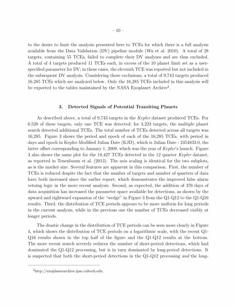
As described above, a total of 9,743 targets in the Kepler dataset produced TCEs. For

6,520 of these targets, only one TCE was detected; for 3,223 targets, the multiple planet

search detected additional TCEs. The total number of TCEs detected across all targets was

16,285. Figure 3 shows the period and epoch of each of the 16,285 TCEs, with period in

days and epoch in Kepler-Modified Julian Date (KJD), which is Julian Date - 2454833.0, the

latter offset corresponding to January 1, 2009, which was the year of Kepler’s launch. Figure

3 also shows the same plot for the 18,427 TCEs detected in the 12 quarter Kepler dataset,

as reported in Tenenbaum et al. (2013). The axis scaling is identical for the two subplots,

as is the marker size. Several features are apparent in this comparison. First, the number of

TCEs is reduced despite the fact that the number of targets and number of quarters of data

have both increased since the earlier report, which demonstrates the improved false alarm

vetoing logic in the more recent analysis. Second, as expected, the addition of 376 days of

data acquisition has increased the parameter space available for detections, as shown by the

upward and rightward expansion of the “wedge” in Figure 3 from the Q1-Q12 to the Q1-Q16

results. Third, the distribution of TCE periods appears to be more uniform for long periods

in the current analysis, while in the previous one the number of TCEs decreased visibly at

longer periods.

The drastic change in the distribution of TCE periods can be seen more clearly in Figure

4, which shows the distribution of TCE periods on a logarithmic scale, with the recent Q1-

Q16 results shown in the top half of the figure and the Q1-Q12 results at the bottom.

The more recent search severely reduces the number of short-period detections, which had

dominated the Q1-Q12 processing, but is in turn dominated by long-period detections. It

is suspected that both the short-period detections in the Q1-Q12 processing and the long-

2http://exoplanetarchive.ipac.caltech.edu.

– 11 –

period detections in the Q1-Q16 processing are dominated by false alarms, and that the

difference in the two populations is due to changes in the false alarm veto algorithms over

the intervening period of TPS development.

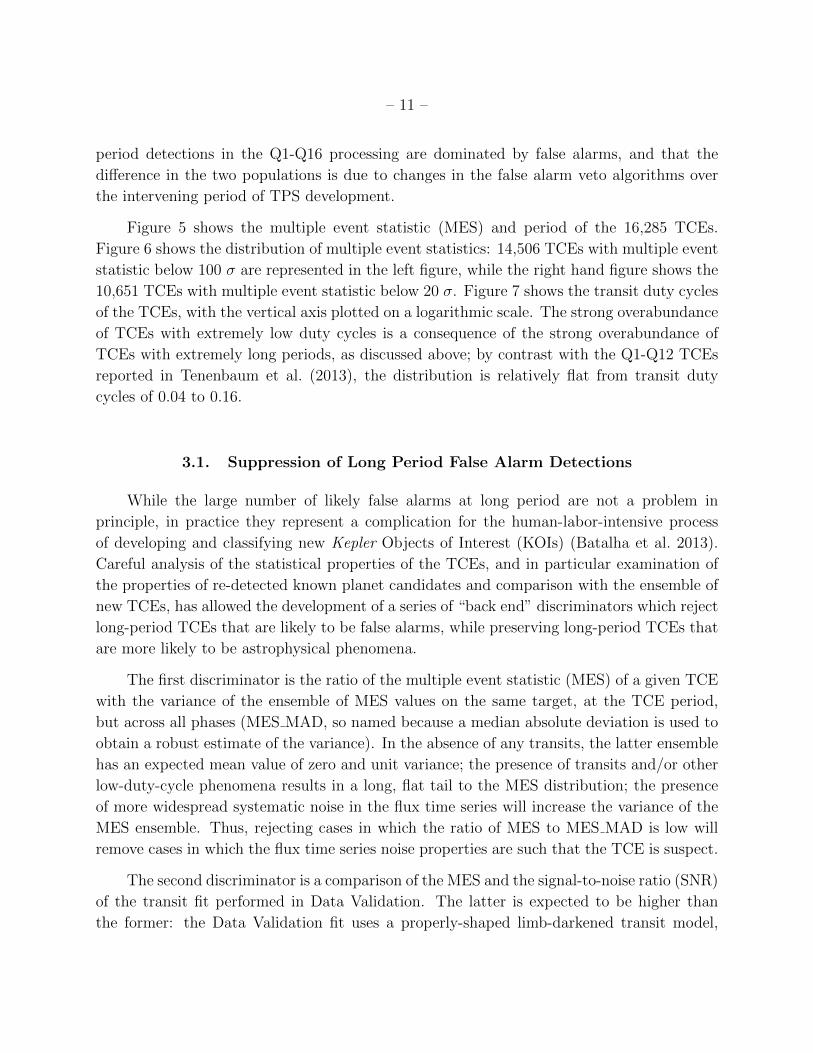
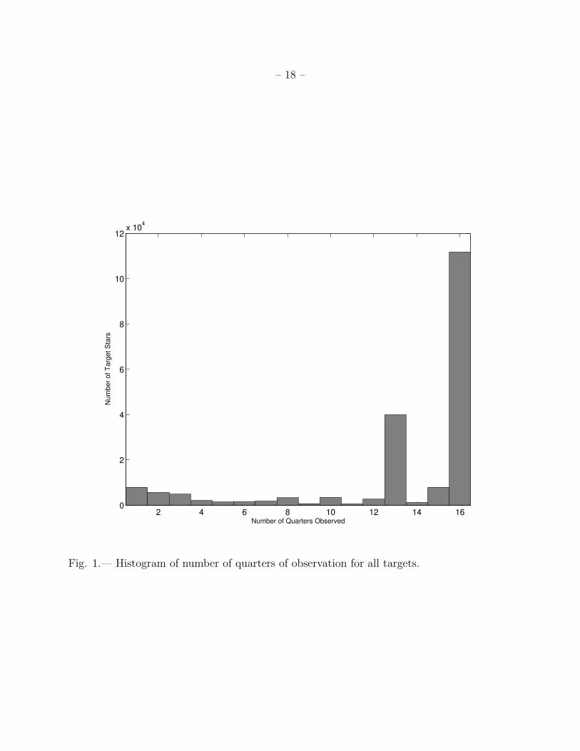
Figure 5 shows the multiple event statistic (MES) and period of the 16,285 TCEs.

Figure 6 shows the distribution of multiple event statistics: 14,506 TCEs with multiple event

statistic below 100 σ are represented in the left figure, while the right hand figure shows the

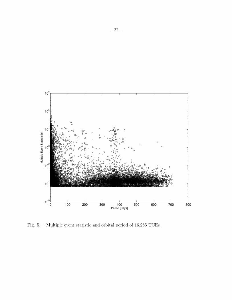
10,651 TCEs with multiple event statistic below 20 σ. Figure 7 shows the transit duty cycles

of the TCEs, with the vertical axis plotted on a logarithmic scale. The strong overabundance

of TCEs with extremely low duty cycles is a consequence of the strong overabundance of

TCEs with extremely long periods, as discussed above; by contrast with the Q1-Q12 TCEs

reported in Tenenbaum et al. (2013), the distribution is relatively flat from transit duty

cycles of 0.04 to 0.16.

3.1. Suppression of Long Period False Alarm Detections

While the large number of likely false alarms at long period are not a problem in

principle, in practice they represent a complication for the human-labor-intensive process

of developing and classifying new Kepler Objects of Interest (KOIs) (Batalha et al. 2013).

Careful analysis of the statistical properties of the TCEs, and in particular examination of

the properties of re-detected known planet candidates and comparison with the ensemble of

new TCEs, has allowed the development of a series of “back end” discriminators which reject

long-period TCEs that are likely to be false alarms, while preserving long-period TCEs that

are more likely to be astrophysical phenomena.

The first discriminator is the ratio of the multiple event statistic (MES) of a given TCE

with the variance of the ensemble of MES values on the same target, at the TCE period,

but across all phases (MES MAD, so named because a median absolute deviation is used to

obtain a robust estimate of the variance). In the absence of any transits, the latter ensemble

has an expected mean value of zero and unit variance; the presence of transits and/or other

low-duty-cycle phenomena results in a long, flat tail to the MES distribution; the presence

of more widespread systematic noise in the flux time series will increase the variance of the

MES ensemble. Thus, rejecting cases in which the ratio of MES to MES MAD is low will

remove cases in which the flux time series noise properties are such that the TCE is suspect.

The second discriminator is a comparison of the MES and the signal-to-noise ratio (SNR)

of the transit fit performed in Data Validation. The latter is expected to be higher than

the former: the Data Validation fit uses a properly-shaped limb-darkened transit model,

– 12 –

including fine adjustment of the transit duration, epoch, and period; the MES in the TCE is

effectively the SNR achieved by fitting a much lower-fidelity, box-shaped model to the same

data. When the ratio of the DV fit SNR to the TCE MES is low, it indicates an event which

does not have a transit-like shape. Note that, for some TCEs, no SNR value was available

due to issues in the Data Validation processing. In these cases, the cut on the SNR-to-MES

ratio was not applied.

Finally, the MES of the TCE can be compared to the minimum MES on the same target

at the TCE period but across all epochs. In the absence of astrophysical signatures, the MES

follows a normal distribution with zero mean and unit variance; consequently, the minimum

multiple event statistic at the TCE period should be a negative value, and should have a

probability distribution given by the negative-valued portion of a Gaussian. The ratio of

the absolute value of the minimum multiple event statistic (henceforth MES MIN) to the

MES of the TCE should therefore be small for a high-quality detection. The presence of

periodic positive excursions in the target flux time series at the TCE period indicate a strong

probability that some phenomenon other than transits is responsible for the TCE.

After analysis of the properties of the discriminators above, we found that it was possible

to remove a significant fraction of the long-period false alarms while preserving the high-

quality TCEs. This is accomplished by rejecting a TCE for which any of the following is

true:

1. MES / MES MAD < 7.1,

2. SNR / MES < 0.6 (for TCEs which have an SNR value available),

3. MES MIN / MES > 0.6.

When these cuts were applied to the Q1-Q12 population of planet candidates, it was

determined that approximately 1% would be rejected and approximately 99% retained. Ap-

plying these cuts to the Q1-Q16 TCEs reduces the number of TCEs to be vetted from 16,285

to 7,959, and of particular importance in this run, from 6,073 to 1,243 with periods of 300

days or more.

3.2. Comparison with Known Kepler Objects of Interest (KOIs)

As in past analyses (Tenenbaum et al. 2012, 2013), we have identified a subset of the

Kepler Objects of Interest (KOIs) which we use as a set of test subjects for the TPS run.

– 13 –

TPS does not receive any prior knowledge about detections on targets; therefore, the re-

detection of objects of interest which were previously detected and classified as valid planet

candidates is a valuable test to guard against inadvertent introduction of significant flaws

into the detection algorithm.

The list of Q1-Q12 KOIs has been analyzed and a set of high-quality “golden KOIs”

identified for comparison to the Q1-Q16 TCEs. This subset of the full KOI list is a repre-

sentative cross-section of all KOIs in the parameters of transit depth, signal-to-noise, and

period, and includes cases which have been identified as eclipsing binaries or astrophysical

false positives.

The “golden KOI” set includes 1,646 KOIs across 1,417 target stars. Figure 8 shows

the distribution of estimated transit depth, signal-to-noise ratio, and period for the “golden

KOIs.” Out of these, 1,372 target stars produced one or more TCE, while 45 target stars

did not. All 45 of the target stars which produced no TCE have one and only one KOI per

target, and the missed KOIs are strongly dominated by short periods: 39 out of 45 have

periods under 3 days, and only 1 out of 45 has a period in excess of 1 quarter. Examination

of the short period failures indicates that they are dominated by a common failure mode,

in which short period transits are mistaken for narrow-band oscillations of the host star

and eliminated by an algorithm which is designed to address such narrow-band oscillations

(this algorithm is discussed briefly in Section 2 of Tenenbaum et al. (2012)). Note that the

oscillations are only removed in instances in which they are strong, i.e., instances in which

a small number of narrow-band resonances dominate the stellar variability relative to more

broad-band variations. As a consequence, the removed transiting planet signatures have

short periods and are strong relative to the background stellar variability. This implies that

the resonance removal is primarily a problem for re-detection of planet candidate signatures

which were detected early in the Kepler Mission, and has little relevance for detection of

weak signals with short periods.

3.2.1. Matching of KOI and TCE Ephemerides

Detection of a TCE on a “golden KOI” target star is a necessary but not sufficient

condition to conclude that TPS is functioning properly. An additional step is that the TCEs

must be consistent with the expected signatures of the KOIs. This is assessed by comparing

the ephemerides of the KOIs and their TCEs, as described in Tenenbaum et al. (2013); the

ephemeris-matching process also implicitly compares the numbers of KOIs and TCEs on

each target star, which exposes cases in which, on a given star, some but not all KOIs were

detected.

– 14 –

Of the 1,601 KOIs on the 1,372 target stars which produced TCEs, it was possible

to find matches for 1,599 of the KOIs. The two KOIs which did not produce TCEs were

KOI 1101.01 (KIC 3245969), and KOI 351.04 (KIC 11442793). KOI 1101.01 is a short-

period candidate (2.84 days), and was most likely removed by the narrow-band oscillation

algorithm; the second candidate on this target, with a period of 11.4 days, was detected

with a correct ephemeris match. KOI 351 is a notorious multi-planet system with significant

transit timing variations (TTVs) ; since TPS requires highly periodic signals to produce a

valid detection, its performance on this system has always been poor. Nonetheless, TPS did

detect KOI 351.03, KOI 351.05, and KOI 351.06 with correct ephemeris matches, though in

the case of 351.05 the match is only approximate (match criterion value of 0.82, indicating

overlap between 82% of the transits in the KOI and the TCE).

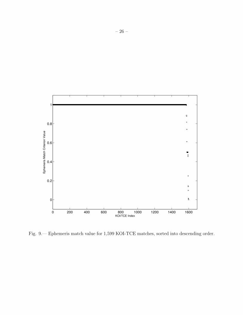
Figure 9 shows the value of the ephemeris match criterion for the 1,599 KOI-TCE

matches, sorted into descending order. A total of 1,569 KOI-TCE matches have a criterion

value of 1.0, indicating that each transit predicted by one ephemeris corresponds to a transit

predicted by the other, to within one transit duration. In these cases, it has been assumed

that TPS correctly detected the “golden KOI” in question and no further analysis was

performed.

In the 30 cases in which the ephemeris match was imperfect, each KOI-TCE match was

manually inspected. The disposition of the results is as follows:

• In 11 cases, the TCE actually matches the KOI, but the value of the match parameter

does not reflect this; in general this is because the KOI ephemeris was derived with

early flight data, requiring extrapolation to determine the transit times late in the

mission and permitting an accumulation of error in the KOI transit timings relative to

the actual timings

• In 13 cases, TPS detected a harmonic or sub-harmonic of the KOI, with a KOI period

twice the TCE period the most common by far

• In 2 cases, TPS detected the planet but produced an incorrect ephemeris due to transit

timing variations (TTVs)

• In 2 cases, TPS detected a known KOI which was different from the “golden KOI” on

the target in question, and which was not itself a “golden KOI”; when all of the KOIs

on a target are part of the “golden KOI” list there is no possibility of such a confusion,

but in cases where some but not all KOIs are on the list this sort of confusion can

happen

• In 2 cases, TPS failed to detect the KOI and the TCE appears to be a false alarm.

– 15 –

In conclusion, out of the 30 KOI-TCE pairs which have imperfect ephemeris matches, only

2 actually constitute a failure of the detection algorithm.

In addition to the TCEs described above, there were 476 TCEs detected on the KOI

targets which are not on the list of “golden KOIs.” The majority of these are known KOIs

which were not included on the “golden KOI” list (i.e., cases in which some of the KOIs on a

given target star were included while others fell below the threshold for inclusion); in other

cases, the unmatched TCE is a secondary eclipse of an eclipsing binary or an occultation of

a large planet behind its host star. In a few cases, these may constitute new detections of

additional planet candidates on stars already known to host one or more such candidates.

3.2.2. Conclusion of TCE-KOI Comparison

Out of 1,646 “golden KOIs” used to demonstrate the validity of the TPS algorithm,

1597 were correctly detected, for a recovery rate of 97.0%. The missed KOIs were largely

overlooked by TPS due to an algorithm which, in removing from the data narrow-band

resonances due to stellar variation, occasionally removes short-period transiting planet sig-

natures. This removal issue is not expected to impact future discoveries of transit signatures

which are weak relative to the overall stellar variability of their host stars.

4. Conclusions

The Transiting Planet Search (TPS) algorithm was used to search photometry data for

197,320 Kepler targets acquired over 4 years of science operations. This resulted in the de-

tection of 16,285 threshold crossing events (TCEs) on 9,743 target stars. The distribution of

TCEs was qualitatively different from those obtained in a similar search utilizing 3 years of

data: the more recent analysis contains a larger proportion of long-period detections which

are considered likely false alarms, but a smaller proportion of short-period false alarms. The

differences are believed to be due to changes made to the TPS algorithm, rather than to

the additional flight data or changes in the data pre-processing algorithms. Out of 1,646

Kepler Objects of Interest (KOIs) used to validate the detection algorithm, 1,597 were cor-

rectly detected; the missed detections were dominated by short-period objects, and a known

limitation of TPS is suspected in these cases.

– 16 –

5. Acknowledgements

Funding for this mission is provided by NASA’s Space Mission Directorate. The contri-

butions of Hema Chandrasekaran continue to be essential in the studies documented here.

A. Determining the Threshold for Positive Outlier Removal

In Section 2.1, an algorithm is described which removes positive outliers from each

flux time series prior to searching same for transits. The algorithm requires a threshold for

removal of the outliers, which is set at 12.3 σ. The rationale behind this value is explained

below.

The most obvious requirement for the positive outlier threshold is that it should, indeed,

address only outliers and not flux values which are merely above the mean value due to

statistical fluctuations. For a whitened flux time series with 69,810 samples, in the limit

of Gaussian statistics, we expect that, on average, 1 sample will lie 4.2 σ above the mean.

Therefore, any threshold which is significantly higher than 4.2 σ can be expected to be

harmless in terms of its effect on sample values which are driven by statistical fluctuations

alone.

Another consideration is that the purpose of removing positive outliers is actually to

suppress the formation of transit-like features in the ring-down of the outliers, since the latter

can lead to false alarm detections. Given a detection threshold of 7.1 σ and a requirement of

at least 3 transits for detection, a negative feature with a significance of 7.1σ ×√

3 = 12.3σ

can exceed the detection threshold when paired with two “transits” which each have a

significance of zero. This implies that a transit-like feature with a significance of 12.3 σ has

a strong probability of triggering a false alarm, and thus our threshold for removing positive

outliers should be set such that any outlier which is likely to have a 12.3 σ transit-like feature

in its ring-down is removed.

Since the ring-down of a positive outlier will always be smaller than the outlier itself,

it follows that removing positive outliers with 12.3 σ significance is more than sufficient to

prevent formation of negative ring-down features with 12.3 σ significance. Since 12.3 σ is

much larger than 4.2 σ, it also follows that this threshold will be benign from the point of

view of ignoring statistical fluctuations. Thus a threshold of 12.3 σ was adopted for positive

outlier removal.

– 17 –

REFERENCES

Allen, B. 2004, Phys. Rev. D 71, 062001

Batalha, N.M., et al. 2013, ApJS, 204, 24

Borucki, W.J., et al. 2010, ApJ, 713, L126

Caldwell, D.A. et al.2012, ApJ713,L92

Christiansen, J.L. et al. 2012, PASP, 124, 1279

Gilliland, R. L., Brown, T. M., Guhathakurta, P., et al. 2000, ApJ, 545, L47

Gilliland, R.L. et al. 2011, ApJS197, 6

Haas, M.R. et al.2010, arXiv:1001.0437

Jenkins, J. M. 2002, ApJ, 575, 493

Jenkins, J.M. et al.2010, arXiv:1001.0258

Jenkins, J.M., et al. 2010, Proc SPIE 7740,77400D

Kirk, B. et al. 2013, in preparation.

Seader, S., et al. 2013, ApJS, 206, 25

Smith, J.C. et al. 2012, PASP124, 1000

Tenenbaum, P. et al. 2012, ApJS199, 24

Tenenbaum, P. et al.2013, ApJS206, 5

Twicken, J.D., et al. 2010b, Proc SPIE 7740, 77401U

Twicken, J.D. et al. 2014, in preparation.

Wu, H. et al. 2010, Proc SPIE 7740, 774019

This preprint was prepared with the AAS LATEX macros v5.2.

– 18 –

2 4 6 8 10 12 14 160

2

4

6

8

10

12x 10

4

Number of Quarters Observed

Nu

mb

er

of

Ta

rge

t S

tars

Fig. 1.— Histogram of number of quarters of observation for all targets.

– 19 –

50 60 70 80 90 100 110 120 130 140 150−0.1

0

0.1

0.2

0.3

Re

lative

Flu

x

50 60 70 80 90 100 110 120 130 140 150−100

0

100

200

300

400

Relative Cadence Number

Wh

ite

ne

d F

lux [

σ]

Fig. 2.— Effect of a positive flux outlier. Top: original flux. Bottom: whitened flux. Note

that whitening introduces a negative outlier to the whitened flux, which can be misconstrued

as a transit. While the resulting negative outlier is much smaller than the original positive

outlier, in this case the negative outlier still has a single event significance of over 27 σ.

– 20 –

100 200 300 400 500 600 7000

200

400

600

800

100 200 300 400 500 600 7000

200

400

600

800

Epoch of First Transit [KJD]

Pe

rio

d [

Da

ys]

Fig. 3.— Top: epoch and period of the 16,285 TCEs detected in Q1-Q16 of Kepler data;

bottom: epoch and period of the 18,427 TCEs detected in Q1-Q12 of Kepler data, as reported

in Tenenbaum et al. (2013). Periods are in days, epochs are in Kepler-modified Julian Date

(KJD), see text for definition.

– 21 –

−0.5 0 0.5 1 1.5 2 2.5 30

200

400

600

800

1000

−0.5 0 0.5 1 1.5 2 2.5 30

200

400

600

800

1000

log10

Period [Days]

Nu

mb

er

of

TC

Es

Fig. 4.— Distribution of TCE periods, plotted logarithmically. Top: 16,285 TCEs in the

Q1-Q16 search. Bottom: 18,427 TCEs in the Q1-Q12 search.

– 22 –

0 100 200 300 400 500 600 700 80010

0

101

102

103

104

105

106

Period [Days]

Mu

ltip

le E

ve

nt

Sta

tistic [

σ]

Fig. 5.— Multiple event statistic and orbital period of 16,285 TCEs.

– 23 –

0 20 40 60 80 1000

500

1000

1500

Nu

mb

er

of

Occu

rre

nce

s

5 10 15 200

50

100

150

200

250

300

Maximum Multiple Event Statistic [σ]

Fig. 6.— Distribution of multiple event statistics. Left: 14,506 TCEs with multiple event

statistic below 100 σ. Right: 10,651 TCEs with multiple event statistic below 20 σ.

– 24 –

0 0.02 0.04 0.06 0.08 0.1 0.12 0.14 0.16 0.180

0.5

1

1.5

2

2.5

3

3.5

4

Transit Duty Cycle

log

10 T

CE

s

Fig. 7.— Transit duty cycles of TCEs.

– 25 –

1 1.5 2 2.5 3 3.5 4 4.5 5 5.50

50

100

150

log10

Transit Depth [PPM]

0.5 1 1.5 2 2.5 3 3.5 40

50

100

150

log10

SNR

Occu

rre

nce

s

−1 −0.5 0 0.5 1 1.5 2 2.5 30

50

100

log10

Period [Days]

Fig. 8.— Parameter distribution of “golden KOIs.” Note use of logarithmic horizontal axes

in all cases.

– 26 –

0 200 400 600 800 1000 1200 1400 1600

0

0.2

0.4

0.6

0.8

1

KOI/TCE Index

Ep

he

me

ris M

atc

h C

rite

rio

n V

alu

e

Fig. 9.— Ephemeris match value for 1,599 KOI-TCE matches, sorted into descending order.