Detection of Enhanced Radar Signal using LMS of Enhanced Radar Signal using LMS K.Anusha Asst.prof...

Detection of Enhanced Radar Signal using LMS K.Anusha Asst.prof

Department of ECE,Raghu Institute of Technology, Visakhapatnam, India.

K.S.L.Venkatesh IV/IV B.E Degree

Department of ECE Raghu Institute of Technology, Visakhapatnam, India.

B.Sai Sasidhar IV/IV B.E Degree


B.Venkatesh IV/IV B.E Degree


Abstract - Adaptive arrays mostly employ phased arrays to automatically sense and eliminate unwanted signals entering the radar's Field of View (FOV) while enhancing reception about the desired target returns. For this purpose, adaptive arrays utilize a rather complicated combination of hardware and require demanding levels of software implementation. Through feedback networks, a proper set of complex weights is computed and applied to each channel of the array. A successful implementation of adaptive arrays depends heavily on two factors: first, a proper choice of the reference signal, which is used for comparison against the received target/jammer returns. A good estimate of the reference signal makes the computation of the weights systematic and effective. On the other hand, a bad estimate of the reference signal increases the array's adapting time and limits the system to impractical (non- real time) situations. Second, a fast (real time) computation of the optimum weights is essential. Thus, the LMS algorithm has been developed for this purpose.

Key words: Linear array, Adaptive, LMS, FOV and Optimum weights.

I. INTRODUCTION

1.1 Linear Arrays: The Figure1. Shows a linear array antenna consisting of identical elements. The element spacing is d (normally measured in wavelength units).

Figure 1. Linear array of equally spaced elements

International Journal of Latest Trends in Engineering and Technology (IJLTET)

Volume 4 Issue 3 September 2014 130 ISSN: 2278-621X

Let element #1 serve as a phase reference for the array. From the geometry, it is clear that an outgoing wave at the nth element leads the phase at the element by , kdsin θ where k= 2π/l The combined phase at the far field observation point is independent of Ø and can be written as

(1) Thus, the electric field at a far field observation point with direction-sine equal to sin θ (assuming isotropic elements) is given by

(2) It follows that the normalized intensity pattern is equal to

(3) The normalized two-way array pattern (radiation pattern) is given by

(4) The radiation pattern G sin(θ) has cylindrical symmetry about its axis sin θ=0 and is independent of the azimuth angle. Thus, it is completely determined by its values within the interval (0 < θ < Ø). The main beam of an array can be steered electronically by varying the phase of the current applied to each array element. Steering the main beam into the direction-sine is accomplished by making the phase difference between any two adjacent elements equal to kd sinθ0. In this case, the normalized radiation pattern can be written as

(5)

If θ0=0 , then the main beam is perpendicular to the array axis, and the array is said to be a broadside array. Alternatively, the array is called an end fire array when the main beam points along the array axis.

II. LEAST MEAN SQUARES (LMS)

Adaptive signal processing evolved as a natural evolution from adaptive control techniques of time varying systems. Advances in digital processing computation techniques and associated hardware have facilitated maturing adaptive processing techniques and algorithms. Consider the basic adaptive digital system shown in Fig. 2.

.

Figure 2. Basic Adaptive system



The system input is the sequence x[k] and its output is the sequence y[k]. What differentiates adaptive from non adaptive systems is that in adaptive systems the transfer function Hk(z) is now time varying. The arrow through the transfer function box is used to indicate adaptive processing (or time varying transfer function).

The sequence d(k) is referred to as the desired response sequence. The error sequence is the difference

between the desired response and the actual response. Remember that the desired sequence is not completely known; otherwise, if it were completely known, one would not need any adaptive processing to compute it. The definition of this desired response is dependent on the system specific requirements.

Many different techniques and algorithms have been developed to minimize the error sequence. Using one

technique over another depends heavily on the operating environment under consideration. For example, if the input sequence is a stationary random process, then minimizing the error signal is nothing more than solving the least mean squares problem. However, in most adaptive processing systems the input signal is a non stationary process. In this section the least mean squares technique is examined. The least mean squares (LMS) algorithm is the most commonly utilized algorithm in adaptive processing, primary because of its simplicity. The time varying transfer function of order L can be written as a Finite Impulse Response (FIR) filter defined by

= (6) The input output relationship is given by the discrete convolution

(7) The goal of the adaptive LMS process is to adjust the filter coefficients toward an optimum minimum mean square error (MMSE).Where X the vector is the input signal sequence. Substituting into

yields

(8) The choice of the convergence parameter µ plays a significant role in determining the system performance. A successful implementation of the LMS algorithm depends on the input signal, the choice of the desired signal, and the convergence Parameter. Much research and effort has been devoted toward selecting the optimal value µ. Nonetheless, no universal value has been found. However, a range for this parameter has been determined to be 0<µ<1.

Often, a normalized value for the convergence parameter µN can be used instead of its absolute value. That is

(9)

Where L is the order of the adaptive FIR filter and s2 is the variance (power) of the input signal. When the input signal is not stationary and its variance is varying with time, a time varying estimate of s2 is used. That is

(10) Where a is a factor selected such that 0< a<1. Finally, Eq. can be written as

(11)



III. THE LMS ADAPTIVE ARRAY PROCESSING

Consider the LMS adaptive array shown in Fig. 3. The difference between the reference signal and the array output constitutes an error signal. The error signal is then used to adaptively calculate the complex weights, using a predetermined convergence algorithm. The reference signal is assumed to be an accurate approximation of the desired signal (or desired array response). This reference signal can be computed using a training sequence or spreading code which is supposed to be known at the radar receiver. The format of this reference signal will vary from one application to another. But in all cases, the reference signal is assumed to be correlated with the desired signal. An increased amount of this correlation significantly enhances the accuracy and speed of the convergence algorithm being used. In this section, the LMS algorithm is assumed.

Figure.3 A linear adaptive array.

In general, the complex envelope of a band pass signal and its corresponding analytical (pre-envelope) signal can be written using the quadrature components pair (xI (t) xt(Q) ). Recall that the quadrature components are related using the Hilbert transform as follows:

(12)

Using this notation, the adaptive output signal, its reference signal and the error signal can also be written using the same notation as

(13)

(14)

(15) Referencing Fig.3, denote the output of the nth array input signal as sn(t) and assume complex weights is given by

(16)

Therefore, the output of the entire adaptive array is

(17) As discussed earlier, one common technique to achieving the MMSE of an LMS algorithm is to use steepest

descent. Thus, the complex weights in the LMS adaptive array are related as defined in . That is,



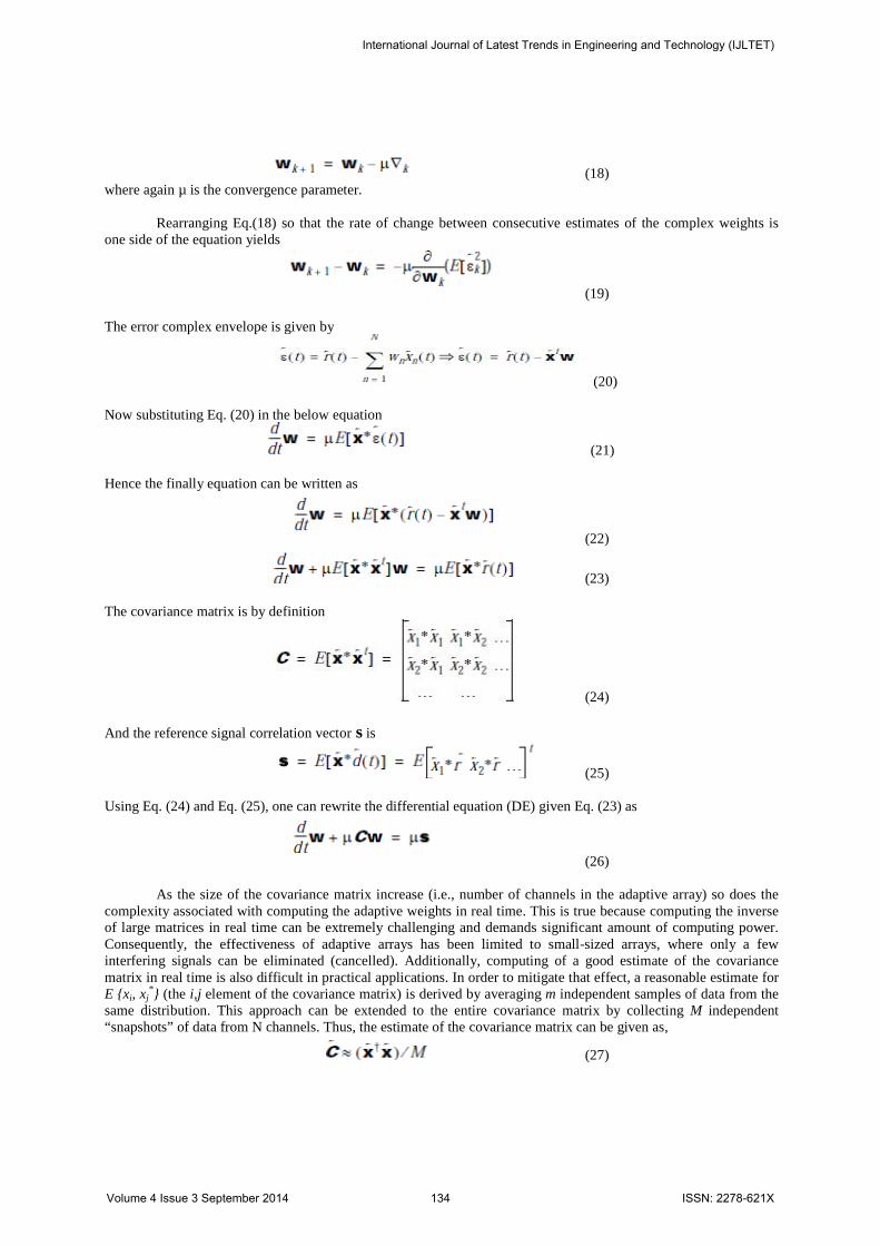
(18) where again µ is the convergence parameter.

Rearranging Eq.(18) so that the rate of change between consecutive estimates of the complex weights is one side of the equation yields

(19) The error complex envelope is given by

(20) Now substituting Eq. (20) in the below equation

(21)

Hence the finally equation can be written as

(22)

(23)

The covariance matrix is by definition

(24)

And the reference signal correlation vector s is

(25)

Using Eq. (24) and Eq. (25), one can rewrite the differential equation (DE) given Eq. (23) as

(26)

As the size of the covariance matrix increase (i.e., number of channels in the adaptive array) so does the complexity associated with computing the adaptive weights in real time. This is true because computing the inverse of large matrices in real time can be extremely challenging and demands significant amount of computing power. Consequently, the effectiveness of adaptive arrays has been limited to small-sized arrays, where only a few interfering signals can be eliminated (cancelled). Additionally, computing of a good estimate of the covariance matrix in real time is also difficult in practical applications. In order to mitigate that effect, a reasonable estimate for E {xi, xj

*} (the i,j element of the covariance matrix) is derived by averaging m independent samples of data from the same distribution. This approach can be extended to the entire covariance matrix by collecting M independent “snapshots” of data from N channels. Thus, the estimate of the covariance matrix can be given as,

(27)



IV. RESULTS

Case (1): Normalized Radiation pattern for linear array (for N=19)

-1 -0.8 -0.6 -0.4 -0.2 0 0.2 0.4 0.6 0.8 10

0.5

1

Arr

ay p

atte

rn

-1 -0.8 -0.6 -0.4 -0.2 0 0.2 0.4 0.6 0.8 1-60

-40

-20

0

sine angle - dimensionless

Pow

er p

atte

rn in

dB

Case (2): Radiation pattern with different Steering angles using Hamming window technique.

-80 -60 -40 -20 0 20 40 60 80-40

-20

0

Steering angle in degrees

An

tenn

a ga

in p

att

ern

in d

B

N = 19; d = 0.5l; q = 0 degrees; Perfect phase shifters

-80 -60 -40 -20 0 20 40 60 80

-40

-20

0


Ant

enn

a g

ain

patt

ern

in d

B N = 19; d = 0.5l; q = 0 degrees; Perfect phase shifters; Hamming window

-80 -60 -40 -20 0 20 40 60 80-30-20-10

010


Ant

enna

gai

n pa

ttern

in d

B

N = 19; d = 0.5l; q = -15 degrees; 3-bits phase shifters

-80 -60 -40 -20 0 20 40 60 80-20

-10

0

10


Ant

enna

gai

n pa

ttern

in d

B

N = 19; d = 0.5l; q = 5 degrees; 3-bits phase shifters; Hamming window

-80 -60 -40 -20 0 20 40 60 80-20

-10

0

10


Ant

enna

gai

n pa

ttern

in d

B

N = 19; d = 0.5l; q = 25 degrees; 3-bits phase shifters; Hamming window



-80 -60 -40 -20 0 20 40 60 80-60

-40

-20

0

Steering angle in degreesA

nten

na g

ain

patte

rn in

dB

N = 19; d = 1.5l; q = 48 degrees; Perfect phase shifters

-80 -60 -40 -20 0 20 40 60 80

-40

-20

0


Ant

enna

gai

n pa

ttern

in d

BN = 19; d = 1.5l; q = 48 degrees; Perfect phase shifters; Hamming window

-80 -60 -40 -20 0 20 40 60 80-40

-20

0


Ante

nna

gain

pat

tern

in d

B

N = 19; d = 1.5l; q = -53 degrees; 3-bits phase shifters

-80 -60 -40 -20 0 20 40 60 80

-40

-20

0


Ante

nna

gain

pat

tern

in d

B

N = 19; d = 1.5l; q = -33 degrees; 3-bits phase shifters; Hamming window

Case (3): Plot for Output response from FIR filter using LMS algorithm.

0 50 100 150 200 250 300 350 400 450 500-2

0

2

Des

ired

resp

onse

m = 0.01; a = 0.1

0 50 100 150 200 250 300 350 400 450 500-5

0

5

Cor

rupt

ed s

igna

l

0 50 100 150 200 250 300 350 400 450 500-2

0

2

time in sec

LMS

out

put



V. CONCLUSION

Case 1. Presents the Normalized Radiation pattern for linear array (for N=19), Case 2. Presents the Radiation pattern with different Steering angles using Hamming window technique. It is observed that in order to reduce the side-lobe levels, the array must be designed to radiate more power toward the centre and much less at the edges. This can be achieved through tapering (windowing) the current distribution over the face of the array. There are many possible tapering sequences that can be used for this purpose. However, as known from spectral analysis, windowing reduces side-lobe levels at the expense of widening the main beam. Thus, for a given radar application, the choice of the tapering sequence must be based on the trade-off between side-lobe reduction and main-beam widening. Finally the detection of the desired signal from the adaptive array and the output response of FIR filter using LMS algorithm presents in case 3.

REFERENCES [1] Barkat, M., Signal Detection and Estimation, Artech House, Norwood, MA,1991. [2] Barton, D. K., Modern Radar System Analysis, Artech House, Norwood, MA,1988. [3] Brookner, E., ed., Practical Phased Array Antenna System, Artech House,Norwood, MA, 1991. . [4] Compton, R. T., Adaptive Antennas, Prentice Hall, Englewood Cliffs, NJ,1988. [5] Gabriel, W. F., Spectral Analysis and Adaptive Array Superresolution Techniques,Proc. IEEE, Vol. 68, June 1980, pp. 654-666. [6] Hamming, R. W., Digital Filters, 2nd edition, Prentice Hall, Englewood Cliffs,NJ, 1983. [7] Meyer, D. P. and Mayer, H. A., Radar Target Detection: Handbook of Theory and Practice, Academic Press, New York, 1973. [8] Poularikas, A. and Ramadan, Z. M., Adaptive Filtering Primer with MATLAB, Taylor & Francis, Boca Raton, FL, 2006. [9] Weiner, M. M., ed., Adaptive Antennas and Recivers, Taylor & Francis, BocaRaton, FL, 2006.



Detection of Enhanced Radar Signal using LMS of Enhanced Radar Signal using LMS K.Anusha Asst.prof...

Documents

Transcript of Detection of Enhanced Radar Signal using LMS of Enhanced Radar Signal using LMS K.Anusha Asst.prof...