Detection and Tracking of Boundary of Unmarked Roads

Young-Woo SeoThe Robotics Institute

Carnegie Mellon UniversityPittsburgh, PA 15213 USA

Email: young-woo.seo@ri.cmu.edu

Ragunathan (Raj) RajkumarDept of Electrical Computer Engineering

Carnegie Mellon UniversityPittsburgh, PA 15213 USAEmail: raj@ece.cmu.edu

Abstract— This paper presents a new method of detectingand tracking the boundaries of drivable regions in road withoutroad-markings. As unmarked roads connect residential placesto public roads, the capability of autonomously driving on sucha roadway is important to truly realize self-driving cars in dailydriving scenarios. To detect the left and right boundaries ofdrivable regions, our method first examines the image regionat the front of ego-vehicle and then uses the appearanceinformation of that region to identify the boundary of thedrivable region from input images. Due to variation in theimage acquisition condition, the image features necessary forboundary detection may not be present. When this happens,a boundary detection algorithm working frame-by-frame basiswould fail to successfully detect the boundaries. To effectivelyhandle these cases, our method tracks, using a Bayes filter, thedetected boundaries over frames. Experiments using real-worldvideos show promising results.

I. INTRODUCTION

This study aims at developing a computer vision algorithmthat detects and tracks the boundaries of drivable regionsappearing on input images. The roads we are particularlyinterested in are paved roads, but no road-markings (e.g.,lane-markings, stop-lines, etc.) are painted, like ones con-necting public roads to residential areas. Figure 1 showsfour examples of such roads. To make self-driving cars trulyuseful, they should be capable of driving on such roads todemonstrate autonomous driving maneuvers from a house,through public roads, to a destination. This work reports theprogress of our effort that develops the perception part ofsuch a driving capability – detecting and tracking of drivableregions’ boundaries.

We assume that, in a given image, the appearance (e.g.,color and texture) of drivable regions would be, with a minorvariation, homogeneous. To understand the characteristicsof the drivable regions’ appearance, we analyze the imagesub-region at the front of ego-vehicle. The blue rectanglesin Figure 1 show examples of such a sampling area. Theidea of analyzing the image region around ego-vehicle tounderstand the characteristics of drivable regions has beenexploited in many outdoor navigation work [1], [2], [3], [4],[5], [6]. However, the actual methods of identifying road-drivable regions are different from one another, e.g.) utilizinglidar scans to define close-range drivable regions [2], using astereo camera to define road plane [3], and using the resultsof vanishing point detection to guide the sampling region [4].They are all similar to each other in that they analyzed thecolor in multi-channels (e.g., Hue-Saturation-Intensity) of thesampling area to extract color patterns of drivable regions.By contrast, our method does not learn the color model of

Fig. 1: Sample images of road without road-markings andthe outputs of the proposed algorithm. A self-driving carshould be capable of driving on roads like the ones appearingon these images. To do so, it is necessary to identifythe boundaries of drivable regions. Red lines represent theoutputs of our boundary detection algorithm and green linesdepict the outputs of our boundary tracking algorithm.

drivable regions because 1) analyzing images in multiplecolor channels requires more resources (e.g., computationaltime and memory space) and 2) learning the color modelis often unreliable in terms of the performance of a colorclassification. Instead our method transforms an input imageinto a bird-eye view image and uses an intensity thresholdingto identify the boundary of drivable regions. Alon et al. alsoused an inverse perspective image to identify the left andright boundaries of off-roads [7].

The performance of image-based algorithms is sensitiveto the variation of the relevant image features’ presence.For example, if the values of image features such as coloror intensity, are drastically changed due to the changesin an image acquisition process, frame-by-frame detectionalgorithms would fail to provide the outputs consistent overframes. To avoid such inconsistent outputs, we develop aBayes filter to track the detected boundaries. To this end, weuse Dickmanns and Mysliwetz’s seminal work, the clothoidmodel of road shape [8] to model the detected boundary anddevelop an unscented Kalman filter (UKF) [9] to implementto track the detected boundaries.

Most work of the drivable region boundary tracking beginswith a boundary detection. For the boundary tracking, theyused the results of boundary detection as measurements. Themajority of boundary tracking work employed the particle fil-ter [10], [11], [12], [13], [14]. To the best of our knowledge,the clothoid (or Euler spiral) is the most widely used modelfor delineating road geometric shape. Some works includingours used the clothoid to model road shape and approximatedactual shapes using cubic polynomials. Using this clothoidmodel, some works aimed at tracking the boundaries of ruralroads [10] and unpaved roads [11], but most of them targetedto track the boundaries of paved roads with road-markings[12], [13], [14].

In what follows, we detail how our method detects theboundaries of roads paved, but no road-markings paintedin Section II-A. And then we describe how our method,using an unscented Kalman filter (UKF), tracks the detectedboundaries over frames in Section II-B. Section III discussesthe finding of the experimental results and Section IV sum-marizes the findings.

II. IDENTIFICATION OF DRIVABLE REGION BOUNDARIESOF ROADS WITHOUT ROAD-PAINTING

This section details how our method 1) detects the leftand right boundaries of roads with no-road-paintings and 2)tracks the detected boundaries over frames.

To detect the boundaries of drivable regions, we first con-vert an input image into a bird-eye view image (or an inverseperspective image). We do this to reduce the computationalcost for image processing1 and to remove any distortioncaused by perspective image acquisition. From an inverseperspective image, our method analyzes the image regionat the front of our vehicle to understand the characteristicsof drivable regions’ appearance. In particular, we determinetwo intensity threshold values to identify the drivable region.Given the results of such a simple, but effective imageanalysis, we identify multiple of road-boundary points fromthe left and right side of ego-vehicle. The detected boundarypoints are then used as measurements for the boundarytracker. We use the clothoid model to model the boundary ofdrivable regions and develop an UKF to track the detectedboundaries.

A. Detection of Drivable Region Boundaries

To detect the boundary of road, we first transform aninput image into an inverse perspective image [15] and thenanalyze a rectangular image region at the front of ego-vehicle to understand the characteristics of drivable regions’appearance. The red rectangle at Figure 2 (b) shows anexample of such a sample image region. This red rectanglecorresponds to the blue rectangle at Figure 2 (a). We dosuch a sampling because we assume that drivable regionsappearing on an input image have similar appearance (e.g.,intensity). Figure 2 (b) shows an example of an inverseperspective image that converts the input image shown atFigure 2 (a). This happens through the transformation, PG =

1The dimension of an inverse perspective image (i.e., 627×711) is smallerthan that of the original image (i.e., 2448×2048).

Fig. 3: Examples of the boundary points. (a) The redcircles represents the detected boundary points on an inverseperspective image. (b) The boundary points detected froman inverse perspective image are projected onto an input,perspective image.

TGI PI , where PG is a point of an inverse perspective image,TGI is the inverse perspective transformation matrix, PI is apoint on the input image.

Using pixels in the sample region, we analyze the intensityof drivable regions and compute the statistics (i.e., mean,µI and standard deviation, σI ) of intensity to choose twointensity thresholds: µI − 3σI and µI + 3σI . We assumethat the intensity of drivable regions follows a Gaussiandistribution, x ∼ N(µ, σ) and choose all the pixels within3σ (intensity values similar to 99% of the sampling area).We apply such an intensity thresholding to the input imageand perform a connected-component analysis to the resultsof the thresholding, to identify a drivable region. Figure 2(c) shows the results of these steps. As the thresholding isnot a fine-tuned technique, the results of the thresholdingis not optimal in that this method does not return a convexpolygon of drivable region. However, as shown in Figure 2(c), executing grouping based on pixels’ connectivity resultsin most of the pixels belonging to the drivable region intothe same pixel group. This technique is fairly simple, butworks effectively in that the pixel group with the largestpixels always corresponds to the drivable region of an inputimage. Figure 2 (c), for instance, shows that our thresholdingmethod returned a pixel group in light blue color at theright front of our vehicle. Although this pixel group hasa couple of elliptical holes in it, the edges of the pixelblob correspond to the boundary of drivable regions. Oncewe find a pixel group corresponding to the drivable region(i.e., the pixel group with largest number of pixels), we scanthrough the pixel group, investigate the n number of rows,and pick two end of points of each investigating row asthe left and the right boundary points. This results in 2nboundary points, B =

{bLj ,b

Rj

}j=1,...,n

, where bL,Rj ∈ R2

is a two-dimensional vector containing the pixel coordinates,bLj(bRj)

= [xLj , yLj ]T

([xRj , y

Rj ]T

). Figure 3 (a) shows the

examples of these detected boundary points in an inverseperspective image and its perspective image (b).

B. Tracking of Drivable Region Boundaries

The previous section describes how our boundary de-tection method works. Our boundary detector analyzes arectangular image sub-region at the front of our car on an in-

Fig. 2: (a) A part of an input image (i.e., the yellow rectangle area) is transformed into a bird-eye view image (or aninverse perspective image) (b) to remove perspective effects and to facilitate image processing. (c) Our algorithm analyzesthe image region at the front of our vehicle and detects drivable-region by applying intensity-thresholding.

Fig. 4: The road-shape model and the measurement model.

verse perspective image and applies an intensity thresholdingto identify drivable image region. A connected-componentgrouping is applied to the result image of intensity thresh-olding and the biggest pixel group is chosen as the drivableimage region. This detection method results in 2n boundarypoints, B =

{bLj ,b

Rj

}j=1,...,n

. This section details how ourboundary tracker models, using these boundary points, theleft and the right boundaries and track, using a Bayes filter,these boundaries over time.

We use the clothoid to model roadway’s geometric shape[8]. A clothoid defines a function of road curvature givenroad (longitudinal) length, κ(l) = c0 + c1l =

∫ l0κ(τ)dτ ,

where c0 is the initial curvature and c1 is the curvaturederivative. Suppose that the starting point of a clothoid is

(x0, y0), where the curvilinear coordinate, l = 0, then eachcoordinate of the curvature function is in fact defined as

x(l) = x0 +

∫ l

0

sin θ(τ)dτ (1)

y(l) = y0 +

∫ l

0

cos θ(τ)dτ (2)

To numerically evaluate these functions, it is required toapproximate them using the Taylor expansions of sin θ andcos θ. The first-order approximation of the clothoid equationsis as

x =1

6c1y

3 +1

2c0y

2 + βy + xoffset (3)

where xoffset is the lateral offset between the boundary andthe vehicle (or boundaries of vehicle body), β is the headingangle with respect to the vehicle’s driving direction, c0 is thecurvature, and c1 is the curvature rate. Figure 4 illustratesthis model. We use this equation to model the boundary ofdrivable region appearing on an image and define the stateof our boundary tracker as:

x = [xoffset, β, c0, c1]T (4)

Algorithm 1 describes the procedure how our methodtracks drivable region boundary. Our tracker takes, as input,ego-vehicle’s speed and the outputs of the boundary detectionmethods described in Section II-A.

We initialize the state and its covariance matrix as

x0 = [100, 0, 0, 0]T (5)

P0 = diag([102, 0.052, 0.012, 0.0012

]T) (6)

Our initialization assumes that the boundary is initiallystraight and located from 100 pixels, laterally away fromego-vehicle. We empirically set those values for initializingP and found that they worked well.

An UKF uses an unscented transformation to model a non-linear dynamics [9]. This often works better than that of Ex-tended Kalman filter, which uses a linearization technique toapproximate a non-linear dynamics using Jacobian. Because

Algorithm 1 UKF for tracking the drivable regions’ bound-aries.Input: vk, ego-vehicle’s speed and

2n boundary points, B ={bLj ,b

Rj

}j=1,...,n

,

Output: xk = [voffset, β, c0, c1]T , an estimate of the road-

shapeFor the left (and the right) boundary, do the following:

1: Given a previous estimate, xk−1 and Pk−1, compute2m+ 1 sigma points and their weights,(χj , wj)← (xk−1,Pk−1, κ)

2: Predict a state and its error covariance,(x−k ,P

−k ) = UnscentTransform(f(χi, wi),Q)

3: Predict a measurement and its error covariance,(zk,Pz) = UnscentTransform(h(χi, wi),R)

4: Compute Kalman gain, Kk = PxzP−1z , where,

Pxz =∑2m+1i=1 wi

{f(χi)− x−

k

}{h(χi)− zk}T

5: for all{bLj (bRj )

}j=1,...,n

∈ B do6: xk = x−

k +Kj(zj − zj)7: Pk = P−

k −KjPjKTj

8: end for

of Jacobian, it may cause a divergence problem [16]. At thestep 1, the unscented transformation begins with generating2m+ 1 sigma points,

χ1 = xk, χi+1 = xk + ui, χi+m+1 = xk − ui, (7)w1 = κ

m+κ , wi+1 = 12(m+κ) , wi+m+1 = 1

2(m+κ) (8)

where m is the dimension of the state, for our case, m = 4,ui is a row vector from UTU = (m+ κ)Pk, κ = 3−m isa constant, and

∑2mi=0 wi = 1.

For the prediction steps 2 and 3, these sigma pointssampled around the current state, xk are used to computethe mean and covariance of the process model, f(x), toapproximate the non-linear process model.

x−k =

2m+1∑i=1

wif(χi) (9)

P−k =

2m+1∑i=1

wi {f(χi)− xk} {f(χi)− xk}T (10)

where x−k and P−

k are the predicted state and its covariance.Using such an unscented transformation, our process model,f(xk) predicts how the shape of a road is changed with anassumption that the acceleration and yaw rate of ego-vehicleare constant during each time step, ∆t.

xk+1 = f(xk) + qk = f(χi, wi)i=1,...,2m+1 + qk (11)

=

1 v∆t 1

2 (v∆t)2 16 (v∆t)3

0 1 v∆t 12 (v∆t)2

0 0 1 v∆t0 0 0 1

xk + qk

where v is a speed of ego-vehicle and qk is noise of theprocess model, qk ∼ N(0,Q).

The measurement model, h(x−k ) = zk also uses the un-

scented transformation to predict the expected measurements

at a given state. The measurement model is defined as

zk = h(x−1k ; y) + rk = h(χi, wi)i=1,...,2m+1 + rk

=1

6c1y

3 +1

2c0y

2 + βy + xoffset (12)

where rk is the noise of the measurement model, rk ∼N(0,R). Figure 4 illustrates the measurement model, wherea crimson, dashed line at the right is a boundary line basedon the expected measurements.

The next step, the step 4 is to compute a Kalman gainthat is used to determine how importantly a measurementis used to estimate the state. When each boundary point isused to estimate the state, the last step updates the state asmuch as the Kalman gain using the innovation (or residual),(zk− zk), the difference between an actual measurement anda predicted measurement.

Figure 5 shows a sequence of detection and trackingoutputs where the benefit of tracking is demonstrated. Someof the detection outputs incorrectly picked up the boundarylocations whereas the tracking outputs correctly delineatedthe boundary of drivable regions on roads without road-paintings.

III. EXPERIMENTS

This section details the settings and results of the experi-ments we carried out to evaluate performance of the proposedalgorithm. The goal of this work is to develop computervision algorithms that accurately detect and reliably trackthe boundaries of drivable regions of the roads with no road-markings. We first detail the experimental setup in SectionIII-A and then discuss the experimental results in SectionIII-B.

A. Experimental Settings

To collect video data, we drove our robotic vehicle [17]on multiple routes of sub-urban regions around Pittsburgh.These video data were obtained under various weather andillumination conditions. One video was recorded in witherwith snow accumulation in the background, another were ob-tained in spring, under fairly gentle illumination conditions,and the last was recorded on an evening in summer.

The vision sensor installed on our vehicle is PointGrey’sFlea3 Gigabit camera, which can acquire an image frameof 2448×2048, maximum resolution at 8Hz. For a faster,real-time processing, we rescaled the original resolution intohalf and used a predefined ROI, x1 = 0, x2 = Iwidth−1,y1 = 1300 and y2 = 1800 for the inverse-perspectivetransformation.2

We implemented the proposed algorithms in C++ withOpenCV libraries. Our implementation of boundary detectionand tracking ran about 10 Hz on a 2.7 GHz Pentium V.For the UKF, we used the Bayes++ package3 to imple-ment our boundary tracker and initialized the state and itserror (or covariance) matrix, x0 = [xoffset, β, c0, c1]

T=

[100, 0, 0, 0]T and P0 = diag

([102, 0.052, 0.012, 0.0012]

),

2These y-values are in the original resolution. If the image is scaled to ahalf of the original, these y-values are scaled as well.

3http://bayesclasses.sourceforge.net/Bayes++.html

Fig. 5: An example sequence of drivable-regions’ boundary detection and tracking.

where the values of x is in pixels, β is in radian, c0, andc1 are dimensionless curvature. In addition, the noises of theprocess model, Q = diag

([102, 0.052, 0.012, 0.0012]

)and

the measurement model, R =[32].

B. Experimental Results

We evaluate resulting boundary delineation in terms ofaccuracy of matching between output and ground truthpixels. To the best of our knowledge, no image data isavailable on identifying boundaries of unmarked road thatwe could use for comparison. Hence, we had to manuallydelineate the image data used for the evaluation.4

To evaluate our results at a pixel-to-pixel level, we utilizedthe method from evaluating performance of object boundarydetection [18]. Similar to [18], we regard the extractionof boundaries as a classification problem of identifyingboundary pixels and of applying the precision-recall metricsusing manually labeled boundaries as ground truth. Precisionis manifested in the fraction of outputs that are true positives;recall is the fraction of correct outputs over true positives. Toevaluate the performance using these metrics, it is necessaryto solve a correspondence problem that determines whichoutput pixels are used to detect which true positive pixels.While resolving such a correspondence problem, we mustcarefully consider a localization error that accounts for the(Euclidean) distance between an output pixel and a groundtruth pixel. Indeed, localization errors are present even inthe ground truth images as well. For resolving the corre-spondence between output pixels and ground truth pixels, weutilized the Berkeley Segmentation Engine’s 5 performanceevaluation scripts. These scripts solve, using Goldberg’s CSApackage, the correspondence problem as a minimum costbipartite assignment problem. Table I shows the performancedifference between the detection and tracking of drivableregions’ boundary, where the F-measure is computed by

4Some video clips about the results are available from http://www.cs.cmu.edu/˜youngwoo/research.html

5The BSE and related information are available at http://www.cs.berkeley.edu/˜fowlkes/BSE/

f = 2×precision×recallprecision+recall . The performance of our detection

algorithm showed a reasonable performance. As expected,the tracking indeed improved our system of identifying theboundaries of unmarked roads 11%.

F-measure Precision RecallDetection 0.70 0.63 0.78Tracking 0.83 0.78 0.89

TABLE I: A precision-recall metric comparison.

Figure 6 shows some example outputs of our boundarydetection and tracking algorithms. The first two rows showsome of the correctly tracked boundary outputs and thelast row show some example outputs that boundaries wereincorrectly identified. Because our boundary detector worksbased on an intensity-thresholding, it occasionally failedto correctly pick up the boundary pixels. Despite of thedetector’s failures, the tracker was able to smooth out incon-sistent outputs from the detector. However, our algorithmsfailed to track the boundaries 1) when our vehicle turned atintersections (e.g., the first image at the last row in Figure 6),2) when the intensities of ground are highly uneven (e.g., theimages between the second and the fourth at the last row),and 3) when the curvature of roads is high (e.g., the lastimage).

IV. CONCLUSIONS AND FUTURE WORK

This paper presented our methods of detecting and track-ing the boundaries of drivable regions of road with noroad-markings. To detect the left and right boundaries ofdrivable regions, our method examines the image region atthe front of ego-vehicle and uses the analyzed appearanceinformation of that region to identify the boundary of thedrivable region from input images. Due to variation in theimage acquisition condition, the image features necessary forboundary detection might not be present. When this happens,a boundary detection algorithm working based on frame-by-frame would fail to successfully detect the boundaries. Toprevent this, our method tracks, using an Unscented Kalman

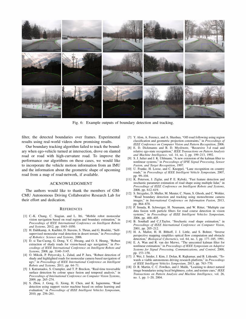
Fig. 6: Example outputs of boundary detection and tracking.

filter, the detected boundaries over frames. Experimentalresults using real-world videos show promising results.

Our boundary tracking algorithm failed to track the bound-ary when ego-vehicle turned at intersection, drove on slantedroad or road with high-curvature road. To improve theperformance our algorithms on these cases, we would liketo incorporate the vehicle motion information from an IMUand the information about the geometric shape of upcomingroad from a map of road-network, if available.

ACKNOWLEDGMENT

The authors would like to thank the members of GM-CMU Autonomous Driving Collaborative Research Lab fortheir effort and dedication.

REFERENCES

[1] C.-K. Chang, C. Siagian, and L. Itti, “Mobile robot monocularvision navigation based on road region and boundary estimation,” inProceedings of IEEE International Conference on Intelligent Robotsand Systems, 2012, pp. 1043–1050.

[2] H. Dahlkamp, A. Kaehler, D. Stavens, S. Thrun, and G. Bradski, “Self-supervised monocular road detection in desert terrain,” in Proceedingsof Robotics: Science and Systems, 2006.

[3] D. si Tue-Cuong, G. Dong, Y. C. Hwang, and O. S. Heung, “Robustextraction of shady roads for vision-based ugv navigation,” in Pro-ceedings of IEEE International Conference on Intelligent Robots andSystems, 2008, pp. 3140–3145.

[4] O. Miksik, P. Petyovsky, L. Zalud, and P. Jura, “Robust detection ofshady and highlighted roads for monocular camera based navigation ofugv,” in Proceedings of IEEE International Conference on IntelligentRobots and Systems, 2011, pp. 64–71.

[5] I. Katramados, S. Crumpler, and T. P. Breckon, “Real-time traversablesurface detection by colour space fusion and temporal analysis,” inProceedings of International Conference on Computer Vision Systems,2009, pp. 265–274.

[6] S. Zhou, J. Gong, G. Xiong, H. Chen, and K. Iagnemma, “Roaddetection using support vector machine based on online learning andevaluation,” in Proceedings of IEEE Intelligent Vehicles Symposium,2010, pp. 256–261.

[7] Y. Alon, A. Ferencz, and A. Shashua, “Off-road following using regionclassification and geometric projection constraints,” in Proceedings ofIEEE Conference on Computer Vision and Pattern Recognition, 2006.

[8] E. D. Dickmanns and B. D. Mysliwetz, “Recursive 3-d road andrelative ego-state recognition,” IEEE Transactions on Pattern Analysisand Machine Intelligence, vol. 14, no. 2, pp. 199–213, 1992.

[9] S. J. Julier and J. K. Uhlmann, “A new extension of the kalman filter tononlinear systems,” in Proceedings of SPIE Signal Processing, SensorFusion, and Target Recognition, 1997.

[10] U. Franke, H. Loose, and C. Knoppel, “Lane recognition on countryroads,” in Proceedings of IEEE Intelligent Vehicle Symposium, 2007,pp. 99–104.

[11] K. Peterson, J. Ziglar, and P. E. Rybski, “Fast feature detection andstochastic parameter estimation of road shape using multiple lidar,” inProceedings of IEEE Conference on Intelligent Robots and Systems,2008, pp. 612–619.

[12] S. Strygulec, D. Muller, M. Meuter, C. Nunn, S. Ghosh, and C. Wohler,“Road boundary detection and tracking using monochrome cameraimages,” in International Conference on Information Fusion, 2013,pp. 864–870.

[13] P. Smuda, R. Schweiger, H. Neumann, and W. Ritter, “Multiple cuedata fusion with particle filters for road course detection in visionsystems,” in Proceedings of IEEE Intelligent Vehicles Symposium,2006, pp. 400–405.

[14] B. Southall and C.J.Taylor, “Stochastic road shape estimation,” inProceedings of IEEE International Conference on Computer Vision,2001, pp. 205–212.

[15] H. A. Mallot, H. H. Blthoff, J. J. Little, and S. Bohrer, “Inverseperspective mapping simplifies optical flow computation and obstacledetection,” Biological Cybernetics, vol. 64, no. 3, pp. 177–185, 1991.

[16] E. A. Wan and R. van der Merwe, “The unscented kalman filter fornonlinear estimation,” in Proceedings of IEEE Symposium on AdaptiveSystems for Signal Processing, Communications, and Control, 2000,pp. 153–158.

[17] J. Wei, J. Snider, J. Kim, J. Dolan, R. Rajkumar, and B. Litkouhi, “To-wards a viable autonomous driving research platform,” in Proceedingsof IEEE Intelligent Vehicles Symposium, 2013, pp. 763–770.

[18] D. R. Martin, C. C. Fowlkes, and J. Malik, “Learning to detect naturalimage boundaries using local brightness, color, and texture cues,” IEEETransactions on Pattern Analysis and Machine Intelligence, vol. 26,no. 1, pp. 1–20, 2004.