arX

iv:p

hysi

cs/0

5020

36 v

1 8

Feb

200

5

Detailed analysis of a pseudoresonantinteraction between cellular flames and

velocity turbulence

V. Karlin

Centre for Research in Fire and ExplosionsUniversity of Central Lancashire, Preston PR1 2HE, UK

Email: VKarlin@uclan.ac.uk

Abstract

This work is dedicated to the analysis of the delicate details of the ef-fect of upstream velocity fluctuations on the flame propagation speed. Theinvestigation was carried out using the Sivashinsky model of cellularisationof hydrodynamically unstable flame fronts. We identified theperturbationsof the steadily propagating flames which can be significantlyamplified overfinite periods of time. These perturbations were used to model the effect ofupstream velocity fluctuations on the flame front dynamics and to study apossibility to control the flame propagation speed.

Key words: hydrodynamic flame instability, Sivashinsky equation, nonmodal am-plification, flame-turbulence interaction

AMS subject classification:35S10, 76E17, 80A25, 65F15

Abbreviated title: Analysis of pseudoresonant flame-turbulence interaction

1 Introduction

Experiments show that cellularisation of flames results in an increase of their prop-agation speed. In order to understand and exploit this phenomenon, we study theevolution of flame fronts governed by the Sivashinsky equation

∂tΦ−2−1 (∂xΦ)2 = ∂xxΦ− (γ/2)∂xH[Φ]+f(x, t), −∞ < x <∞, t > 0(1)

with the force termf(x, t). HereΦ(x, t) is the perturbation of the plane flamefront, H[Φ] = π−1

∫ ∞

−∞(x − ξ)−1Φ(ξ, t)dξ is the Hilbert transformation, and

γ = 1 − ρb/ρu is the contrast in densities of burnt and unburnt gasesρb andρu respectively. Initial perturbationΦ(x, 0) is given.

The equation without the force term was obtained in [1] as an asymptoticmathematical model of cellularisation of flames subject to the hydrodynamic flameinstability. The force term was suggested in [2] in order to account for the effect ofthe upstream turbulence on the flame front. It is equal to the properly scaled turbu-lent fluctuations of the velocity field of the unburned gas. In[3] and [4] equation(1) was further refined in order to include effects of the second order inγ. How-ever, as mentioned in [4], this modification can be compensated upon a Galileantransformation combined with a nonsingular scaling. Thus,we have chosen toremain within the first order of accuracy inγ of the original Sivashinsky model(1) as it should have the same qualitative properties as the more quantitativelyaccurate one.

The asymptotically stable solutions to the Sivashinsky equation withf(x, t) ≡0 corresponding to the steadily propagating cellular flames do exist and are givenby formula

ΦN,L(x, t) = VN,Lt+ 2

N∑

n=1

ln | cosh 2πbn/L− cos 2πx/L|, (2)

discovered in [5]. Here, realL > 0 and integerN from within the range0 ≤N ≤ NL = ceil(γL/8π + 1/2) − 1 are otherwise arbitrary parameters. Also,VL = 2πNL−1 (γ − 4πNL−1), andb1, b2, . . . , bN satisfy a system of nonlinearalgebraic equations available elsewhere. Functions (2) have a distinctive set ofNcomplex conjugate pairs of poleszn = ±ibn, n = 1, . . . , N and are called thesteady coalescent pole solutions respectively.

The steady coalescent pole solutions (2) with the maximum possible numberN = NL of the poles were found to be asymptotically, fort → ∞, stable if thewavelength of the perturbations does not exceedL, see [6]. However, in spite oftheir asymptotic stability, there are perturbations of these solutions which can behugely amplified over finite intervals of time resulting in significant transients, see

2

[7]. These perturbations are nonmodal, because they cannotbe represented by thesingle eigenmodes of the linearised Sivashinsky equation.In what follows we areinterested in solutions (2) withN = NL and retain the indexL only. Also, in allreported calculationsγ = 0.8.

In this work we calculate the most amplifiable nonmodal perturbations to theasymptotically stable cellular solutions of the Sivashinsky equation and use themto investigate the response of the flame front to forcing. In particular, we study theeffect of stochastic forcing or noise. The investigation ofthe effect of noise in theSivashinsky equation was carried out numerically and the observations were rein-forced by the analytical analysis of an approximation to thelinearised Sivashinskyequation suggested in [8].

2 The largest growing perturbations

SubstitutingΦ(x, t) = ΦL(x, t) + φ(x, t) into (1) for f(x, t) ≡ 0 and linearisingit with respect to theL-periodic perturbationsφ(x, t), one obtains

∂tφ = (∂xΦL)∂xφ+ ∂xxφ− (γ/2)∂xH[φ] = ALφ,

φ(x, 0) = Φ(x, 0) − ΦL(x, 0).(3)

The operatorAL generates the evolution operatoretAL , which provides the solu-tion to (3) in the formφ(x, t) = etALφ(x, 0).

Assuming that the polar decomposition of the evolution operator does exist,we write it as

etAL = U(t)S(t), (4)

whereU(t) is a partially isometric andS(t) =[(etAL

)∗etAL

]1/2is the nonnega-

tive self-adjoint operator, see e.g. [9]. The partial isometry of U(t) implies that itpreserves the norm when mapping between the sets of values of

(etAL

)∗andetAL ,

i.e. ‖U(t)φ‖ = ‖φ‖. Then, under certain conditions,‖φ(x, t)‖ = ‖S(t)φ(x, 0)‖and for the2-norm the sup

φ(x,0)∈D(etAL){‖S(t)φ(x, 0)‖ ×‖φ(x, 0)‖−1} is equal to

the largest eigenvalueσ1(t) of S(t). This eigenvalue is associated with the eigen-vectorψ1(x, t) of S(t).

The eigenvectorsψα(x, t) of S(t) are mutually orthogonal at any given timet = t∗ and can be used as a basis in the space of the admissible initial conditions

φ(x, 0) =∞∑

α=1

cα(0, t∗) ×ψα(x, t∗). Then, the associated eigenvaluesσα(t∗) pro-

vide the magnitudes of amplification of theψα(x, t∗) components of the initialconditionφ(x, 0) by the time instancet∗. Note, that for (3) the2-norm of the per-turbationφ(x, t) is just its energy and that the eigenvaluesσα(t), α = 1, 2, . . . and

3

eigenvectorsψα(x, t) of S(t) are the singular values and the right singular vectorsof etAL respectively.

According to [10], the Fourier imageAL of the operatorAL is defined by the(k, l)-th entry of its double infinite (−∞ < k, l <∞) matrix

(AL)k,l =

(−4π2

L2k2 +

πγ

L|k|

)δk,l +

8π2

L2l sign(k − l)

NL∑

n=1

e−2πbn|k−l|/L, (5)

whereδk,l is the Kronecker’s symbol. By limiting our consideration tothe firstKharmonics, we approximate our double infinite matrixAL with the (2K + 1) ×(2K + 1) matrix A(K)

L , whose entries coincide with those ofAL for −K ≤ k, l ≤K. Then, the matrixetA

(K)L ≈ etAL can be effectively evaluated by the scaling and

squaring algorithm with a Pade approximation. Eventually, the required estima-tions ofσα(t) and Fourier images ofψα(x, t) can be obtained through the singular

value decomposition (SVD) ofetA(K)L , see e.g. [11].

Indeed, if the SVD ofetA(K)L is given by

etAL(K)

= W(t)D(t)V(t)∗, (6)

whereW(t), V(t) are unitary andD(t) is the nonnegative diagonal matrix, thenthe matrices

U(t) = W(t)V(t)∗, S(t) = V(t)D(t)V(t)∗ (7)

satisfy the adequate finite-dimensional projection of the polar decomposition (4)and the eigenvaluesσα(t), α = 1, 2, . . . and eigenvectorsψα(x, t) of S(t) arejust the singular values and the Fourier syntheses of the right singular vectors of

etAL(K)

respectively.Graphs showing dependence of a few largest singular values of etAL versus

time are shown in Fig. 1. One may see that values ofσ1,2(t) for large enought match the estimation of the largest possible amplification of the perturbationsφ(x, t) obtained in [7] by a different method. An even more impressive observa-tion is that the dimension of the subspace of the significantly amplifiable pertur-bations is very low. Perturbations of only two types can be amplified by about106

times.The initial conditionsφ(x, 0), which would be the most amplified once by

t∗ = 100, 200, 300 and103, i.e.ψα(x, t∗), are depicted in Fig. 2. The dominatingsingular modesψα(x, t) stabilize to some limiting functions fort > 300. Forexample, their graphs fort = 500 and t = 103 are indistinguishable in Fig. 2.However, they vary in time significantly whent < 300 and for t = 200 the

4

0 500 1000 1500 200010

−2

100

102

104

106

t

σ α(t)

Figure 1: Twelve largest singular values ofetAL .

associated amplificationσ1,2(200) is already about103, thoughψ1,2(x, 200) doesnot coincide with neitherψ1,2(x, 103) norψ3,4(x, 103). Thus, the dependence ofψα on time makes the dimension of the subspace of perturbations, which can beamplified say about103 times much higher than two in contrast to what couldbe concluded from the graphs in Fig. 1. This illustrates the complicatedness ofstudies of the effect of transient amplification on short time scalest < 300.

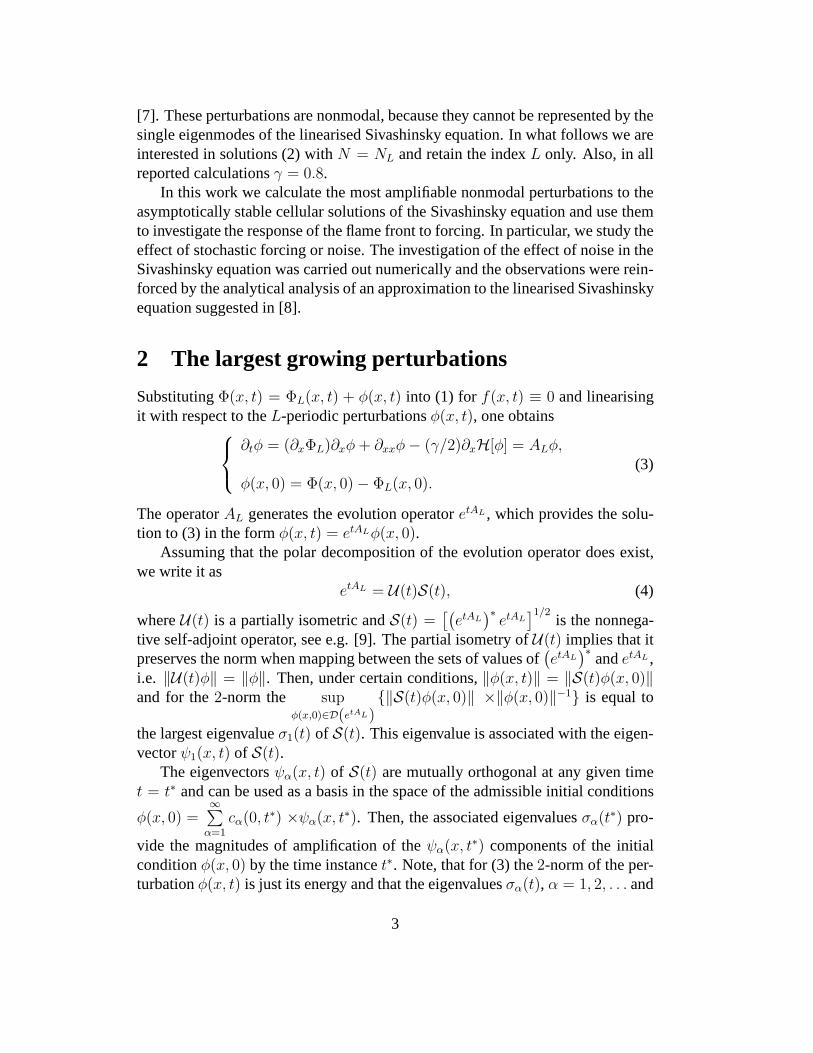
Fourier components ofψ1(x, t∗) andψ2(x, t

∗) for t∗ = 103 are depicted in Fig.3.

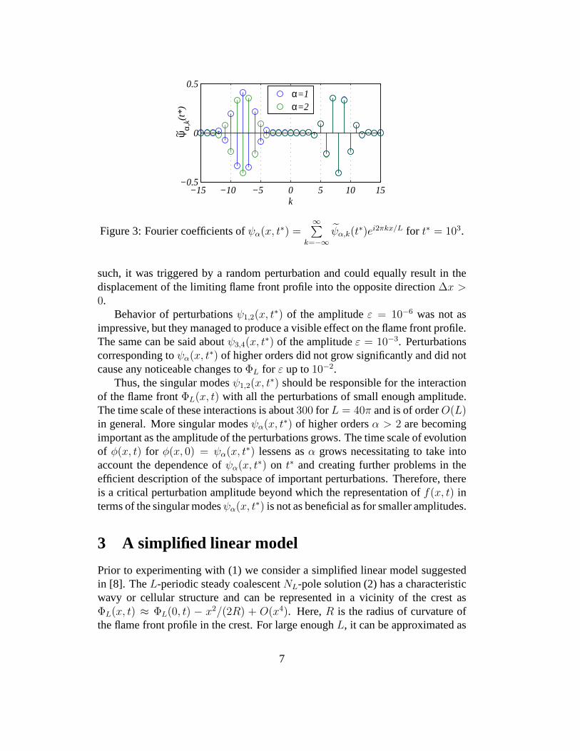
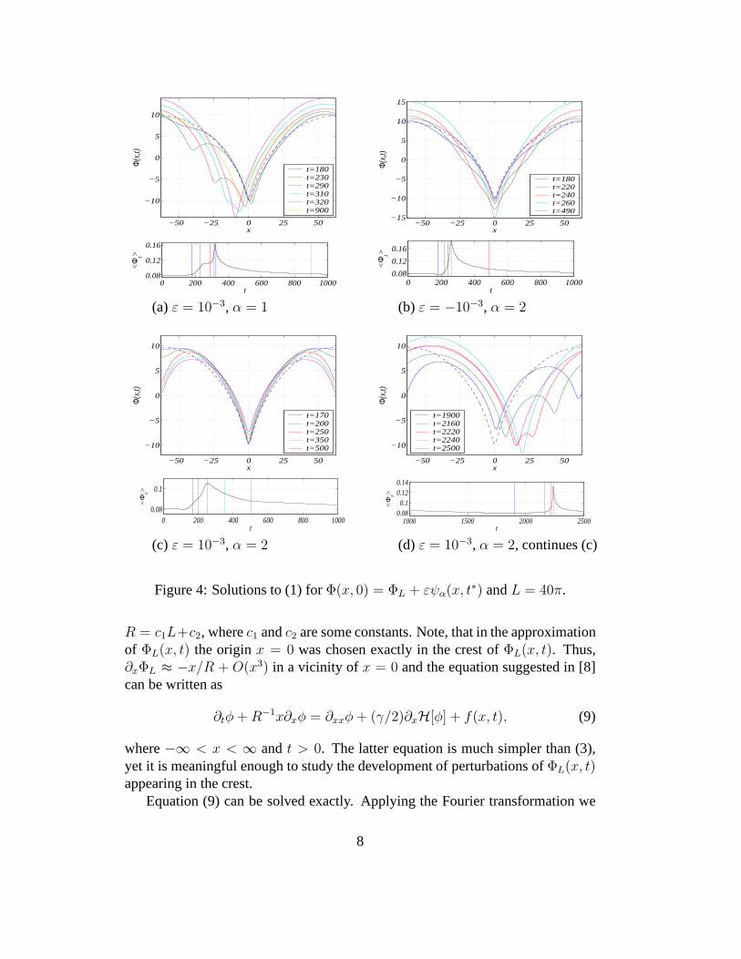
Evolution of the perturbations, which grow the most and is governed by thenonlinear Sivashinsky equation, is illustrated in Fig. 4. All the profiles weredisplaced vertically in order to compensate for steady propagation of flames insuch a way that their spatial averages are equal to zero. Matching graphs of thespatially averaged flame propagation speed

< Φt >=1

L

L/2∫

−L/2

∂tΦ(x, t)dx, (8)

are shown as well. The initial conditions wereΦ(x, 0) = ΦL(x, 0) + εψα(x, t∗),whereε = ±10−3, α = 1, 2, andt∗ = 103. The computational method used inthis work was presented in [12].

The asymmetric singular modeψ1(x, t∗) results in appearance of a small cusp

to the left or to the right from the trough ofΦL(x, 0) depending on the sign ofε. After the cusp merges with the trough, the flame profile converges slowly toΦL(x + ∆x, t), wheresign(ε)∆x > 0. For a positiveε = 10−3 the effect isillustrated in Fig. 4. Graphs ofΦ(x, t) for ε = −10−3 are exact mirror reflectionsof those depicted in 4(a) and graphs of< Φt > are exactly the same.

5

−50 −25 0 25 50−1

−0.5

0

0.5

1

x

ψ 1(x,t)

−50 −25 0 25 50−1

−0.5

0

0.5

1

x

ψ 2(x,t)

−50 −25 0 25 50−1

−0.5

0

0.5

1

x

ψ 4(x,t)

−50 −25 0 25 50−1

−0.5

0

0.5

1

x

ψ 3(x,t)

−50 −25 0 25 50−1

−0.5

0

0.5

1

x

ψ 6(x,t)

−50 −25 0 25 50−1

−0.5

0

0.5

1

x

ψ 5(x,t)

Figure 2: Right singular vectors ofetAL corresponding to the six largestσα(t) fort = 100 (cyan),200 (green),300 (blue), and103 (red).

The symmetric singular modeψ2(x, t∗) produces two symmetric dents moving

towards the trough on both sides of the profile ifε < 0, see Fig. 4(b). Byt ≈ 500the flame profile returns very closely toΦL(x, t). For ε > 0 two small cuspsmove towards the boundaries of the computational domain creating a quasi-steadystructure shown in Fig. 4(c) fort = 270. This structure survives untilt ≈ 1800,but eventually bifurcates, see Fig. 4(d), and the solution converges toΦL(x +∆x, t), ∆x < 0. It looks like the bifurcation in question is associated with thelack of the asymptotic stability of the intermediate quasi-steady structure. As

6

−15 −10 −5 0 5 10 15−0.5

0

0.5

k

ψα

,k(t

*)~

α=1α=2

Figure 3: Fourier coefficients ofψα(x, t∗) =∞∑

k=−∞

ψα,k(t∗)ei2πkx/L for t∗ = 103.

such, it was triggered by a random perturbation and could equally result in thedisplacement of the limiting flame front profile into the opposite direction∆x >0.

Behavior of perturbationsψ1,2(x, t∗) of the amplitudeε = 10−6 was not as

impressive, but they managed to produce a visible effect on the flame front profile.The same can be said aboutψ3,4(x, t

∗) of the amplitudeε = 10−3. Perturbationscorresponding toψα(x, t∗) of higher orders did not grow significantly and did notcause any noticeable changes toΦL for ε up to10−2.

Thus, the singular modesψ1,2(x, t∗) should be responsible for the interaction

of the flame frontΦL(x, t) with all the perturbations of small enough amplitude.The time scale of these interactions is about300 for L = 40π and is of orderO(L)in general. More singular modesψα(x, t∗) of higher ordersα > 2 are becomingimportant as the amplitude of the perturbations grows. The time scale of evolutionof φ(x, t) for φ(x, 0) = ψα(x, t∗) lessens asα grows necessitating to take intoaccount the dependence ofψα(x, t∗) on t∗ and creating further problems in theefficient description of the subspace of important perturbations. Therefore, thereis a critical perturbation amplitude beyond which the representation off(x, t) interms of the singular modesψα(x, t∗) is not as beneficial as for smaller amplitudes.

3 A simplified linear model

Prior to experimenting with (1) we consider a simplified linear model suggestedin [8]. TheL-periodic steady coalescentNL-pole solution (2) has a characteristicwavy or cellular structure and can be represented in a vicinity of the crest asΦL(x, t) ≈ ΦL(0, t) − x2/(2R) + O(x4). Here,R is the radius of curvature ofthe flame front profile in the crest. For large enoughL, it can be approximated as

7

−50 −25 0 25 50

−10

−5

0

5

10

x

Φ(x,

t)

t=180t=230t=290t=310t=320t=900

−50 −25 0 25 50−15

−10

−5

0

5

10

15

x

Φ(x,

t)

t=180t=220t=240t=260t=490

0 200 400 600 800 10000.08

0.12

0.16

t

<Φ

t>

0 200 400 600 800 10000.08

0.12

0.16

t

<Φ

t>

(a) ε = 10−3, α = 1 (b) ε = −10−3, α = 2

−50 −25 0 25 50

−10

−5

0

5

10

x

Φ(x,

t)

t=170t=200t=250t=350t=500

−50 −25 0 25 50

−10

−5

0

5

10

x

Φ(x,

t)

t=1900t=2160t=2220t=2240t=2500

0 200 400 600 800 10000.08

0.1

t

<Φ

t>

1000 1500 2000 25000.080.1

0.120.14

t

<Φ

t>

(c) ε = 10−3, α = 2 (d) ε = 10−3, α = 2, continues (c)

Figure 4: Solutions to (1) forΦ(x, 0) = ΦL + εψα(x, t∗) andL = 40π.

R = c1L+c2, wherec1 andc2 are some constants. Note, that in the approximationof ΦL(x, t) the originx = 0 was chosen exactly in the crest ofΦL(x, t). Thus,∂xΦL ≈ −x/R + O(x3) in a vicinity of x = 0 and the equation suggested in [8]can be written as

∂tφ+R−1x∂xφ = ∂xxφ+ (γ/2)∂xH[φ] + f(x, t), (9)

where−∞ < x < ∞ andt > 0. The latter equation is much simpler than (3),yet it is meaningful enough to study the development of perturbations ofΦL(x, t)appearing in the crest.

Equation (9) can be solved exactly. Applying the Fourier transformation we

8

obtain

∂tF [φ] −R−1ξ∂ξF [φ] = −(4π2ξ2 − πγ|ξ| − R−1

)F [φ] + F [f ](ξ, t), (10)

which is a linear non-homogeneous hyperbolic equation of the first order. Usingthe standard method of characteristics its exact solution can be written as follows

F [φ](ξ, t) = G(ξ, t)F [φ(0)](|ξ|et/R)+

t∫

0

G(ξ, t−τ)F [f ][|ξ|e(t−τ)/R, τ

]dτ, (11)

whereG(ξ, t) = et/R−2π2R(e2t/R−1)ξ2+πγR(et/R−1)|ξ|, (12)

and F [f ](ξ, t) =∫ ∞

−∞f(x, t)e−i2πxξdx denotes the Fourier transformation of

f(x, t).If the initial condition is a single harmonicsφ(0)(x) = cos(2πξ0x + ϕ) and

f(x, t) ≡ 0, then

φ(x, t) = e−2π2R(1−e−2t/R)ξ20+πγR(1−e−t/R)ξ0 cos

(2πξ0xe

−t/R + ϕ). (13)

The infinite time limit of (13) is equale−2π2Rξ20+πγRξ0 cosϕ and is reached ef-

fectively on the time scale of orderO(R). This time limit attains its maximumeγ2R/8 cosϕ for ξ0 = ξ∗ = γ/(4π), matching the asymptotic estimation of [8].Note that the wave number of the largest Fourier componentk∗ of bothψ1(x, t

∗)andψ2(x, t

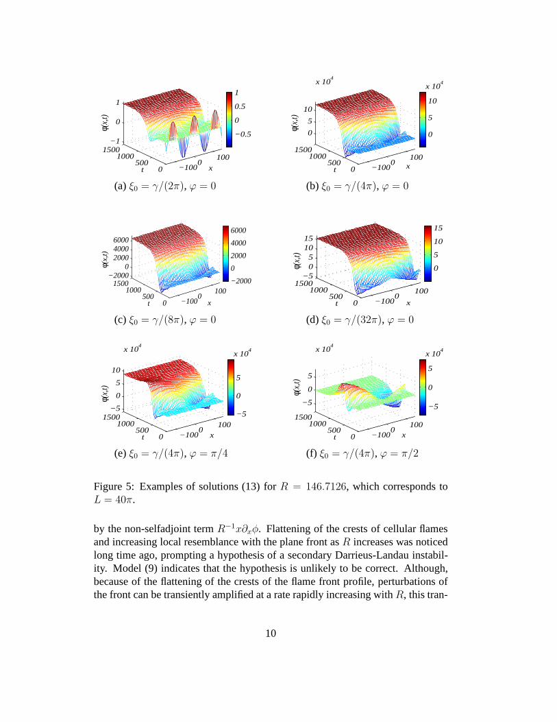
∗) for t∗ > 300 is equal toξ∗ = k∗/L = γ/(4π) as well, see Fig. 3.A few graphical examples of function (13) are given in Fig. 5.Note that the ar-gument of the cosine in (13) depends on time, which means thateven if the initialconditionφ(0)(x) is a linear combination of mutually orthogonal cosine harmon-ics, then the solutionφ(x, t) will remain a linear combination of cosine harmonicsfor t > 0, but those harmonics will no longer be mutually orthogonal.This ex-plains why the most amplified perturbations are formed by linear combinations ofa few initially orthogonal harmonics and approximateψ1,2(x, t

∗) asymptoticallyfor L→ ∞.

Behaviour of (13) is in a sharp contrast with the evolution ofthe single har-monics perturbations of the plane flame front

φ(x, t) = e(−4π2ξ20+πγξ0)t cos(2πξ0x+ ϕ), (14)

which grow infinitely if ξ0 < γ/(4π) or decay otherwise. They are governed bythe equation associated with a self-adjoint differential operator, which is obtainedfrom (9) upon removal of the termR−1x∂xφ. Solution (14) does not result from(13) forR → ∞, but is only equivalent to it whent/R ≪ 1. The difference be-tween (13) and (14) is an explicit illustration of the nonnormality of (9) introduced

9

−1000

100

0500

10001500

−1

0

1

xt

φ(x,

t)

−0.5

0

0.5

1

−1000

100

0500

10001500

0

5

10

x 104

xt

φ(x,

t)

0

5

10

x 104

(a) ξ0 = γ/(2π), ϕ = 0 (b) ξ0 = γ/(4π), ϕ = 0

−1000

100

0500

10001500

−20000

200040006000

xt

φ(x,

t)

−2000

0

2000

4000

6000

−1000

100

0500

10001500

−505

1015

xtφ(

x,t)

0

5

10

15

(c) ξ0 = γ/(8π), ϕ = 0 (d) ξ0 = γ/(32π), ϕ = 0

−1000

100

0500

10001500

−5

0

5

10

x 104

xt

φ(x,

t)

−5

0

5

x 104

−1000

100

0500

10001500

−5

0

5

x 104

xt

φ(x,

t)

−5

0

5

x 104

(e) ξ0 = γ/(4π), ϕ = π/4 (f) ξ0 = γ/(4π), ϕ = π/2

Figure 5: Examples of solutions (13) forR = 146.7126, which corresponds toL = 40π.

by the non-selfadjoint termR−1x∂xφ. Flattening of the crests of cellular flamesand increasing local resemblance with the plane front asR increases was noticedlong time ago, prompting a hypothesis of a secondary Darrieus-Landau instabil-ity. Model (9) indicates that the hypothesis is unlikely to be correct. Although,because of the flattening of the crests of the flame front profile, perturbations ofthe front can be transiently amplified at a rate rapidly increasing withR, this tran-

10

sient amplification is entirely different from the infinite growth of perturbationsin the Darrieus-Landau instability of plane flames. Moreover dynamics of pertur-bations in the case of cellular flames does not converge to that of the plane onescontinuously in the limitR → ∞.

Solution (11), (12) forφ(x, 0) = e−px2, p > 0 can be represented in a closed

form as well. Routine integration yields

φ(x, t) =π√pae

tR

+ b2−4π2x2

4a

{cos

πbx

a+ ℜ

[e

iπbxa erf

(b+ i2πx

2√a

)]}, (15)

where

a = a(t) = 2π2R(e2t/R − 1

)+ π2e2t/R/p, b = b(t) = πγR

(et/R − 1

).

(16)The result is illustrated in Fig. 6, where case (c) corresponds to the maximumgrowing perturbation of typeφ(x, 0) = e−px2

and initial conditionφ(x, 0) = δ(x)was used in (d). The solution formula in the latter case is given by (15) withp for-mally replaced byπ and it also should be used witha = a(t) = 2π2R

(e2t/R − 1

)

andb exactly the same as in (16).The steady coalescent pole solutions to the Sivashinsky equation correspond

to the flame fronts propagating steadily with the velocity exceedingub = 1 byVL, see e.g. [13]. Addition of the perturbationφ(x, t) results in a change in thevelocity of propagation by the value of the space average of∂tφ, which we denote<φt>. The correction provided by theφ(x, t) is only valid in a small vicinityof the crest ofΦL(x, t) . In sequel, the correction of the speed<φt> is onlyvalid for a small region−ε ≤ x ≤ ε of the flame front in a vicinity of the crestof ΦL(x, t). Hence, for our simplified linear model we define the increaseof theflame propagation speed as follows:

<φt>=1

2ε

ε∫

−ε

∂tφdx ≈ ∂tφ|x=0 . (17)

For the single harmonics solution (13) the expression for<φt> is obvious andis illustrated in Fig. 7. These graphs demonstrate high sensitivity of <φt> tothe wavelength of the perturbation. The phase, or location of the perturbation, isimportant as well.

4 The effect of noise

According to the results of Section 2, the forcing in the Sivashinsky equation canbe decomposed into the most amplifiable nonmodal component and the orthogo-nal complement. The latter can be neglected reducing spatio-temporal stochastic

11

(a)p = 1/R (b) p = R

(c) p = 0.0765 (d) φ(x, 0) = δ(x)

Figure 6: Examples of solutions (15), (16) forR = 146.7126, which correspondstoL = 40π.

0 500 1000 15000

100

200

300

t

<φ t>

ξ = γ/4πξ = γ/3πξ = γ/6π

Figure 7: Averaged increase of the local flame propagation speed<φt> for solu-tions (13),ϕ = 0.

noise to the appearance of a sequence of the most growing perturbationsψαm(x, t∗),

12

1 ≤ αm ≤ α∗ = α∗(f0) at a set of time instancestm,m = 0, 1, 2, . . .:

f(x, t) ≈ f0

∞∑

m=0

ψαm(x, t∗)δ(t− tm), 1 ≤ αm ≤ α∗ = α∗(f0). (18)

Thus, the amplitude of noisef0, alongside with the averages and the standarddeviations oftm+1 − tm andαm,m = 0, 1, 2, . . . are the only essential parametersof such a representation of noise.

The impulse-like noise (18) is used here for the sake of simplicity. Somearguments towards its validity were suggested in [2]. More sophisticated andphysically realistic models of temporal noise characteristics can be used with (1)as well.

If f0 ≪ σ−11 (t∗) then noise is not able to affect the flame at all and can be

completely neglected. This case can be referred to as the noiseless regime. On theother hand, iff0 is comparable with the amplitudea of the background solutionΦL(x, t), then almost all components of noise will be able to disturb the flameand thef(x, t) in (1) should be treated as a genuine spatio-temporal stochasticfunction. This is the regime of the saturated noise.

Eventually, there is an important transitional regime whenthe noise amplitudef0 is at least of order ofσ−1

1 (t∗), but still much smaller thana. In this case only thedisturbances with a significant component in the subspace spanned by the linearcombinations ofψα(x, t∗), 1 ≤ α ≤ α∗ have a potential to affect the solution.All other disturbances can be neglected and the forcef(x, t) in the Sivashinskyequation (1) can be approximated by (18) with a finite value ofα∗. We wouldlike to stress that though such representation of noise is correct for noise of anyamplitude, apparently it is only efficient iff0 < σ−1

α∗ (t∗) ≪ a, whereα∗ is smallenough.

4.1 Noise in the linear model

A random point-wise set of perturbations uniformly distributed in time and in theFourier space is a suitable model for both the computationalround-off errors anda variety of perturbations of physical origins. We are adopting such a model inour analysis in the following form

f(x, t) =

M(t)∑

m=1

am cos(2πξmx+ ϕm)δ(t− tm), (19)

wheream, tm, ξm, andϕm are non-correlated random sequences. It is assumedthat t1 ≤ t2 ≤ · · · ≤ tm ≤ · · · ≤ tM(t) ≤ t, 0 ≤ ϕm ≤ 2π, and ξm ≥0, m = 1, 2, . . . ,M(t). Availability of the exact solution (15) makes it also

13

possible to study an alternative noise model based on elementary perturbationsame

−pm(x−xm)2 , which are local in physical space.Using (11), (12) for the zero initial condition, the exact solution to (9), (19)

can be written as

φ(x, t) =

M(t)∑

m=1

ame−2π2R[1−e−2(t−tm)/R]ξ2

m+πγR[1−e−(t−tm)/R]ξm

× cos[2πξme

−(t−tm)/Rx+ ϕm

]. (20)

The expression for<φt> is obvious, see (17), and is illustrated in Fig. 8. Herewe generated random sequences of the time instancestm with a given frequencyF = M(T )/T on a time intervalt ∈ [0, T ]. Values of the wave numberξm and ofthe amplitudeam were also randomly generated and uniformly distributed withincertain ranges. According to the formula for<φt>, the effect of the phase shiftϕm just duplicates theam. Therefore, its value was fixed asϕm ≡ 0.

If values ofam are uniformly distributed in[−1, 1], then the time average of<φt> is obviously zero, because of the linearity of the problem. In the Sivashinskyequation this effect is compensated by the nonlinearity. The cusps generated bythe perturbations of opposite signs move into opposite directions along the flamesurface, see Section 2, though they both contribute into thespeed positively. Thiseffect of the nonlinearity can be mimicked by restricting the range of possiblevalues of the amplitudes, e.g.am ∈ [0, 1], as this can be seen in Fig. 8.

0 1 2 3 4 5

x 104

0

1000

2000

3000

t

<φ t>

0 1 2 3 4 5

x 104

0

1000

2000

3000

t

<φ t>

(a)F = 1, am, ξm ∈ [0, 1] (b) F = 1/33, am ∈ [0, 1],ξm ≡ γ/(4π)

Figure 8: The effect of noise (19) on<φt> for L = 40π.

Figure 8(b) shows that the increase of<φt> seen in Fig. 8(a) can be matchedby using only the largest growing perturbations with much smaller frequency,which is quite expected in virtue of the linearity of the problem. The amplitude offluctuations in Fig. 8(a) is noticeably less than in Fig. 8(b). This is attributed tothe smoothing effect of the less growing perturbations.

14

Because of the linearity of the problem in question, the effect ofF = M(T )/TandL on<φt> is straightforward. In particular, the value of<φt> raises up toabout4×108 for L = 80π and other parameters the same as in Fig. 8(a). It shouldbe noticed however that because of the limitationam ≥ 0 the quantity<φt> doesno longer represent the increase of propagation speed of theflame, but is just ameasure of the rate of transient amplification of perturbations. Figure 9 illustratesthe point, see also [7] and [12].

0 1 2 3 4 5

x 104

0

2

4

x 108

t

<φ t>

Figure 9: The effect of noise (19) on<φt> for L = 80π, F = 1, am ∈ [0, 1], andξm ∈ [0, 1].

Direct studies of the effect of noise in the Sivashinsky equation necessitate useof numerical simulations. However, because of the intrinsic discontinuity of noise,such DNS are hampered with very low accuracy of approximations questioningthe validity of numerical solutions. In this work we used explicit solutions (20)in order to validate DNS of (9) and, in sequel, of (1). The DNS of (9), (19) wascarried out using a spectral method. The delta functionδ(t−tm) was approximatedby (π∆t)−1/2e−(t−tm)2/∆t with a small enough∆t≪ 1/F . The calculations haveshown that discrepancies between (20) and its numerical counterparts obtainedwith the same sets oftm, am, andξm might be noticeable in a neighbourhood ofthe time instancest ≈ tm. Although, the averaged characteristics like<φt> werequite accurate. So, this linear model validates the DNS of the forced Sivashinskyequation at least in relation to the averaged flame propagation speed.

4.2 The Sivashinsky equation

We carried out a series of computations of (1), (18) withΦL(x, t) as initial con-dition and with a variety of parameters of the noise term. Up to twelve basisfunctionsψα(x, 103), whereα was uniformly distributed in the interval1 ≤ α ≤α∗ ≤ 12, were used. The sign off0 in (18) was either plus or minus for everymwith the equal probability1/2. The delta functionδ(t− tm) was approximated by(π∆t)−1/2e−(t−tm)2/∆t with a small enough value of∆t.

15

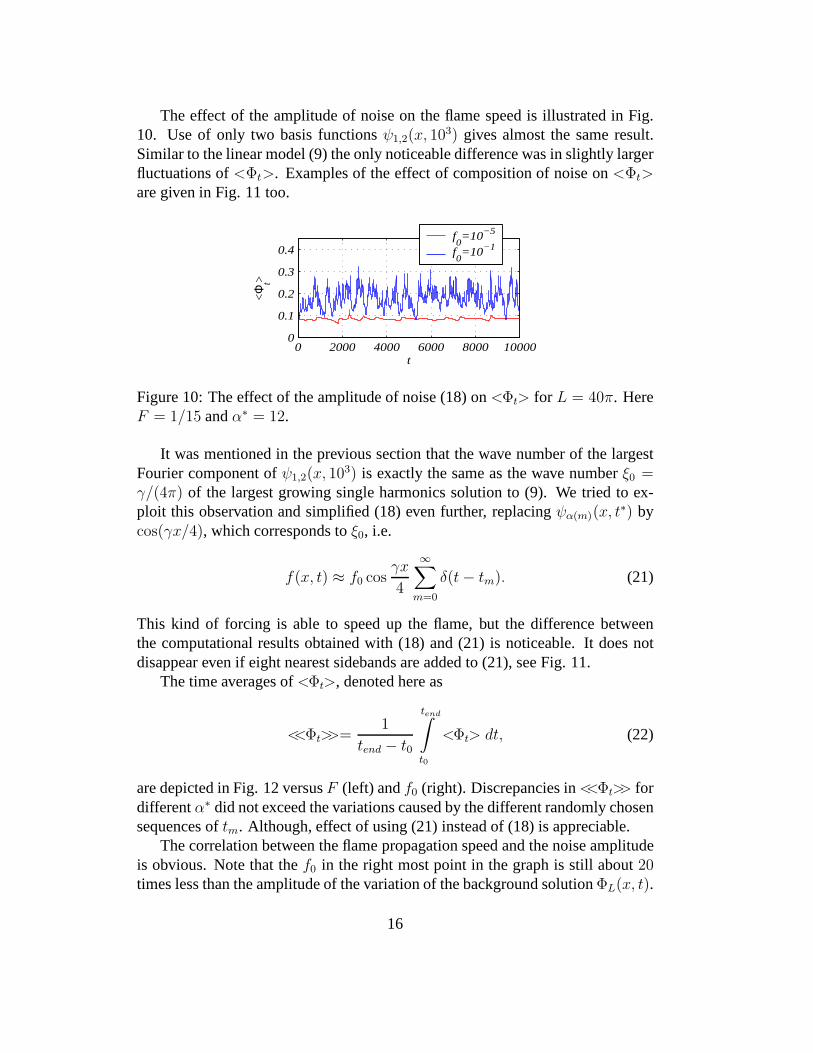
The effect of the amplitude of noise on the flame speed is illustrated in Fig.10. Use of only two basis functionsψ1,2(x, 103) gives almost the same result.Similar to the linear model (9) the only noticeable difference was in slightly largerfluctuations of<Φt>. Examples of the effect of composition of noise on<Φt>are given in Fig. 11 too.

0 2000 4000 6000 8000 100000

0.1

0.2

0.3

0.4

t

<Φt>

f0=10−5

f0=10−1

Figure 10: The effect of the amplitude of noise (18) on<Φt> for L = 40π. HereF = 1/15 andα∗ = 12.

It was mentioned in the previous section that the wave numberof the largestFourier component ofψ1,2(x, 103) is exactly the same as the wave numberξ0 =γ/(4π) of the largest growing single harmonics solution to (9). We tried to ex-ploit this observation and simplified (18) even further, replacingψα(m)(x, t

∗) bycos(γx/4), which corresponds toξ0, i.e.

f(x, t) ≈ f0 cosγx

4

∞∑

m=0

δ(t− tm). (21)

This kind of forcing is able to speed up the flame, but the difference betweenthe computational results obtained with (18) and (21) is noticeable. It does notdisappear even if eight nearest sidebands are added to (21),see Fig. 11.

The time averages of<Φt>, denoted here as

<<Φt>>=1

tend − t0

tend∫

t0

<Φt> dt, (22)

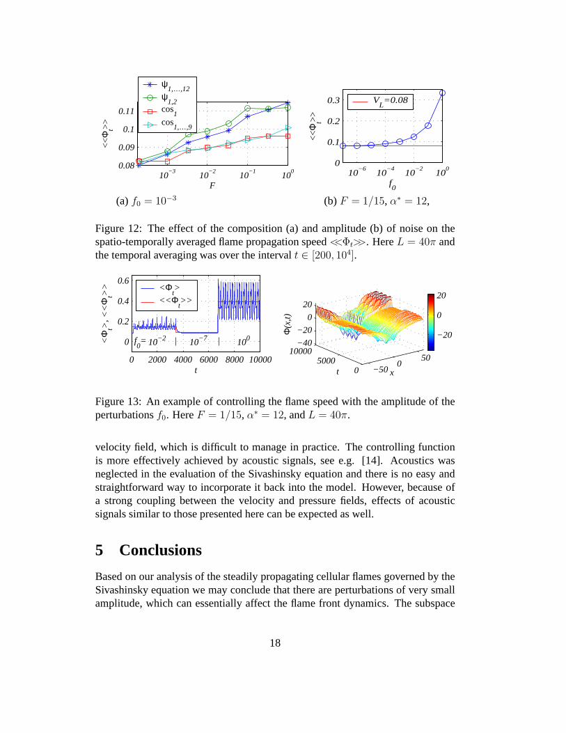
are depicted in Fig. 12 versusF (left) andf0 (right). Discrepancies in<<Φt>> fordifferentα∗ did not exceed the variations caused by the different randomly chosensequences oftm. Although, effect of using (21) instead of (18) is appreciable.

The correlation between the flame propagation speed and the noise amplitudeis obvious. Note that thef0 in the right most point in the graph is still about20times less than the amplitude of the variation of the background solutionΦL(x, t).

16

0 5000 100000.05

0.1

0.15

0.2

t

<φ t>

ψ1,2

, F=1/1000

0 5000 100000.05

0.1

0.15

0.2

t

<φ t>

ψ1,2

, F=1/100

0 5000 100000.05

0.1

0.15

0.2

t

<φ t>

ψ1,2

, F=1/10

0 5000 100000.05

0.1

0.15

0.2

t<

φ t>

ψ1,2

, F=1

0 5000 100000.05

0.1

0.15

0.2

t

<φ t>

ψ1,…,12

, F=1/10

0 5000 100000.05

0.1

0.15

0.2

t

<φ t>

cos1,…,9

, F=1/10

Figure 11: Examples of the effect of the composition of noiseon <Φt > forf0 = 10−3 andL = 40π.

In accordance with the idea developed in this paper, the value of<<Φt>> isdetermined by the productσ1f0. It was shown in [7] thatσ1 ∝ eO(L), resultingin <<Φt>>=<<Φt>> (eO(L)f0). Thus, the data shown in Fig. 12 are at least in aqualitative agreement with the dependence of<<Φt>> onL, which was obtainedin [7] for a fixed noise amplitudef0 ≈ 10−16 associated with the computationalround-off errors.

Eventually, in Fig. 13 we presented the results of an attemptto control theflame propagation speed using our special perturbationsψα(x, t∗) of properly se-lected amplitudes. Graphs of<Φt > and<<Φt >> are shown in the left andnumerical solutionΦ(x, t) corresponding to this controlling experiment is illus-trated in the right. The fluctuations of the obtained flame propagation speed arelarge indeed, but at least, they appear in quite a regular pattern.

In this paper noise or forcing in (1) represents the turbulence of the upstream

17

10−3

10−2

10−1

100

0.08

0.09

0.1

0.11

F

<<Φ

t>>

ψ1,…,12

ψ1,2

cos1

cos1,…,9

10−6

10−4

10−2

100

0

0.1

0.2

0.3

f0

<<Φ

t>>

VL=0.08

(a) f0 = 10−3 (b) F = 1/15, α∗ = 12,

Figure 12: The effect of the composition (a) and amplitude (b) of noise on thespatio-temporally averaged flame propagation speed<<Φt>>. HereL = 40π andthe temporal averaging was over the intervalt ∈ [200, 104].

0 2000 4000 6000 8000 10000

0

0.2

0.4

0.6

t

<Φ

t>,

<<

Φt>

>

f0= 10−2 | 10−7 | 100

<Φt>

<< Φt>>

−500

50

05000

10000−40

−20

0

20

xt

Φ(x

,t)

−20

0

20

Figure 13: An example of controlling the flame speed with the amplitude of theperturbationsf0. HereF = 1/15, α∗ = 12, andL = 40π.

velocity field, which is difficult to manage in practice. The controlling functionis more effectively achieved by acoustic signals, see e.g. [14]. Acoustics wasneglected in the evaluation of the Sivashinsky equation andthere is no easy andstraightforward way to incorporate it back into the model. However, because ofa strong coupling between the velocity and pressure fields, effects of acousticsignals similar to those presented here can be expected as well.

5 Conclusions

Based on our analysis of the steadily propagating cellular flames governed by theSivashinsky equation we may conclude that there are perturbations of very smallamplitude, which can essentially affect the flame front dynamics. The subspace

18

formed by these special perturbations is of a very small dimension and its basis canbe used for an efficient representation of the upstream velocity turbulence. Theseare the very perturbations which cause the increase of the flame propagation speedin numerical experiments. Hence, theoretically, they can be used to model certainregimes of flame-turbulence interaction and to control the flame propagation speedon purpose.

Acknowledgements

The research presented in this paper was supported by the EPSRC grantGR/R66692.

References

[1] G.I. Sivashinsky.Acta Astronautica, 4:1177–1206, 1977.

[2] G. Joulin.Combust. Sci. Tech., 60:1–5, 1988.

[3] G. Joulin and P. Cambray.Combust. Sci. Tech., 81:243–256, 1992.

[4] P. Cambray and G. Joulin. 24th Symp (Int) Combust, 61–67,Combust Inst,1992.

[5] O. Thual, U. Frisch, and M. Henon.Le J. de Phys., 46(9):1485–1494, 1985.

[6] D. Vaynblat and M. Matalon.SIAM J. Appl. Math., 60(2):679–702, 2000.

[7] V. Karlin. Proc. Combust. Inst., 29(2):1537–1542, 2002.

[8] G. Joulin.J. Phys. France, 50:1069–1082, 1989.

[9] I.C. Gohberg and M.G. Krein.Introduction to the Theory of LinearNon-selfadjoint Operators. AMS, Providence, Rhode Island, 1969.

[10] V. Karlin. Math. Meth. Model. Appl. Sci., 14(8):1191–1210, 2004.(Preprint arXiv: physics/0312095, December, 2003 athttp://arxiv.org).

[11] G.H. Golub and C.F. van Loan.Matrix Computations. The Johns HopkinsUniversity Press, 1989.

[12] V. Karlin, V. Maz’ya, and G. Schmidt.J. Comput. Phys., 188(1):209–231,2003.

19

[13] M. Rahibe, N. Aubry, and G.I. Sivashinsky.Combust. Theory Modelling,2(1):19–41, 1998.

[14] C. Clanet and G. Searby.Physical Review Letters, 80(17):3867–3870, 1998.

20