1

Designing E-commerce Supply Chains: a stochastic facility-location approach

A. Pagès-Bernaus1, H. Ramalhinho2, A. A. Juan3, L. Calvet3

(1) adela.pages@matematica.udl.cat, Dept. of Mathematics, University of Lleida, Spain (2) helena.ramalhinho@upf.edu, Dept. of Economics and Business, Universitat Pompeu Fabra, Spain

(3) {ajuanp, lcalvetl}@uoc.edu, IN3 – Dept. of Computer Science, Open University of Catalonia, Spain

Abstract: E-commerce activity has been increasing during the last years, and this trend is expected to continue in the near future. E-commerce practices are subject to uncertainty conditions and high variability in customers’ demands. Considering these characteristics, we propose two facility-location models that represent alternative distribution policies in e-commerce (one based on outsourcing and another based on in-house distribution). These models take into account stochastic demands as well as more than one regular supplier per customer. Two methodologies are then introduced to solve these stochastic versions of the well-known capacitated facility location problem. The first one is a two-stage stochastic programming approach that makes use of an exact solver. However, we show that this approach is not appropriate for tackle large-scale instances due to the computational effort required. Accordingly, we also introduce a ‘simheuristic’ approach that is able to deal with large-scale instances in short computing times. An extensive set of benchmark instances contribute to illustrate the efficiency of our approach, as well as its potential utility in modern e-commerce practices. Keywords: E-commerce, supply chain management, capacitated facility location problem, stochastic combinatorial optimization, simheuristics, stochastic programming.

1. Introduction Consumer behavior is moving from traditional offline shopping to online shopping experiences. According to some experts, the percentage of individuals ordering goods or services over the Internet in developed countries is steadily increasing, reaching a noticeable share of all commerce during the last years. Many factors have propelled the e-commerce revolution, among others: better search engines linked to retailers, programs focused in building confidence by improving online payment services, faster delivery services, strong marketing strategies, etc. In the following years, revenues coming from the e-commerce market are expected to grow annually at a rate of 9% in Europe, 7% in the United States, and 13% in Asia (Statista 2016). This increase in e-commerce activity not only generates new business opportunities, but it also arises some challenges that enterprises must face when designing their distribution networks.

One noticeable characteristic of online sales is the high variability in customers’ demands, which must be incorporated in the supply chain design. In fact, it is expected that future demand from online channels will grow together with the number of transactions driven by: (a) the increase in the number of users –also motivated by the dissemination of mobile access to the Internet (Criteo 2016); (b) a change in the shopping habits –shopping is no longer bounded by time or space constraints; and (c) new sectors entering the online shopping market. Another factor that affects demand is the public acceptance of marketing campaigns focused in boosting online shopping at specific dates, such as the “cyber-Monday” or other special offers that only apply to online shopping.

2

One of the strategic decisions that e-commerce enterprises must face is the location of their facilities or distribution centers (DCs). Notice that this decision has an impact on the daily logistics activity and, consequently, on the customers’ quality of service. In the context of e-commerce, this paper focuses on providing support to online distributors on how to select the DC locations, and how to perform the subsequent assignment of customers to these facilities. In particular, the study presented here was motivated by the requirements of a distributor offering products online to their customers (small business such as restaurants, grocery stores, etc.), although it is quite general and could be extended to many other e-commerce scenarios (mainly of B2B nature). This distributor wants to define its supply chain considering some specific aspects:

• Each customer should be assigned to more than one DC on a regular basis (e.g., in Figure 1, customer i is assigned to facilities A and B). In terms of inventory, layout, and transportation, it is important to know which customers are served from each DC. In traditional business, it is common to have each customer assigned to only one DC. The possibility of having two or more ‘regular’ providers adds flexibility to absorb the demand fluctuations and, accordingly, to achieve a lower delivery cost. The decrease of this cost may be due to the following factors: (i) an increase in the probability of having enough capacity to serve a new customer’s order –without requiring outsourcing; and (ii) a higher flexibility in choosing, for each new order, the DC that offers the lowest delivery cost.

• When none of the regular DCs have enough capacity to satisfy a new customer’s order, other delivery strategies should be explored. The first one considers using an outsourcing policy (e.g., facility D in Figure 1). Usually, there exists a high cost associated with this outsourcing service. However, there are some cases in which outsourcing may be a reasonable delivery option (e.g., in the case of a low-quantity order placed by a customer who is far away from any of its non-regular DCs). The second strategy considers servicing the customer in-house from a non-regular DC (e.g., facility C in Figure 1). Typically, this option will represent a higher transportation cost than using the regular DCs, but it will be generally cheaper than outsourcing.

Figure 1. A schematic representation of the problem being considered

Thus, this paper deals with a rich and realistic version of the facility location problem (FLP), a well-known combinatorial optimization problem (Klose and Drexl 2005, Melo et al. 2009). The

3

FLP has usually been applied to the design of supply chains in a traditional business context. Here, we consider an application motivated by the e-commerce industry. The goal of this work is to study this supply chain design problem and to analyze the impact of different delivery policies in the presence of uncertainty. Since the capacity at each DC is limited, the problem is modeled as a capacitated FLP (CFLP) with stochastic demands. The main contributions of the paper are:

• To present a formal model for the stochastic CFLP in which each customer not only has a random demand but also a reduced number of regular providers. A stochastic programming model is described for each of the two policies considered. Then, both models are solved using the Cplex commercial solver for small-scale instances.

• To propose a ‘simheuristic’ algorithm to solve the stochastic CFLP in the case of large-size instances. Simheuristics constitute a family of algorithms that combine a metaheuristic framework with simulation techniques to address stochastic combinatorial optimization problems in a natural way (Juan et al. 2015a, 2015b). In particular, our solving approach is based on the SimILS framework proposed by Grasas et al. (2016), which integrates Monte Carlo simulation techniques into the iterated local search (ILS) metaheuristic framework (Lourenço et al. 2010, Juan et al. 2014b).

• To evaluate the impact of the two proposed distribution policies (in-house vs. outsourcing), as well as their differences in terms of cost. In order to analyze this impact, a set of computational experiments are performed. The solutions provided by the algorithm are compared against those obtained with the Cplex solver –whenever the latter can be obtained.

The rest of this paper is organized as follows: Section 2 reviews some of the existing literature on the CFLP, including both the deterministic and the stochastic variants; Section 3 presents the formal models describing the CFLP variants considered in this paper; Section 4 provides a description of our simheuristic approach for solving the models; Section 5 includes an extensive set of computational experiments; Section 6 extends the analysis of the obtained results; finally, Section 7 outlines the main conclusions of this work and provides some suggestions for future research.

2. Related Works The study of how e-commerce impacts on the design of supply chains is a relevant topic in current business. However, most publications refer to the last part of the supply chain –e.g., the last-mile delivery (Morganti et al. 2014), the re-design of the batching rules and delivery policies of online orders (Zhang et al. 2016), the adequacy of government programs to eliminate barriers (Gessner and Snodgrass 2015), or the environmental implications of a dual –both traditional and online– channel strategy (Carrillo et al. 2014). For a broader picture, the reader is referred to Siddiqui and Raza (2015), who offer a survey of the e-commerce literature from a supply-chain perspective and identify both gaps and trends. The authors analyze 165 articles focusing on five dimensions: topic-of-study, unit-of-analysis, research perspective, and research method. They highlight the growing number of works involving e-supply chain modeling, design and/or implementation, while only a few authors focus on outsourcing issues. Moreover, it is stated that markets are becoming increasingly uncertain and that the competitiveness is growing fast. In this context, we are interested in developing models and methods that support strategic decisions at the time of planning the location of physical facilities, i.e., the so called mega e-fulfillment centers (Morganti et al. 2014), considering a high variability in the customers’ demands.

The popularity of FLPs is due to the large number of application areas they cover, ranging from logistics to computer and telecommunication networks. Some interesting surveys can be found in Balinski and Spielberg (1969), Revelle et al. (1970), Guignard and Spielberg (1977),

4

Krarup and Pruzan (1983), Revelle et al. (2008), and Melo et al. (2009). The simplest version of FLPs is the well-known uncapacitated FLP or UFLP (Verter 2011), where a set of locations are selected and each customer is allocated to the closest available facility –since these do not have capacity limitations. Many extensions of the UFLP have appeared with the aim of modeling more realistic situations (Klose and Drexl 2005). One of the most common characteristics added to this model is the capacity limit of the facilities. For the CFLP, customers’ demands and capacity limits are commonly provided as input parameters.

Since facility location decisions are usually a long-term investment, one important extension is the inclusion of uncertainty. Some of the parameters in a FLP model –such as future demands or costs–, are difficult to predict, and estimates may significantly differ from actual values. Such variations may have an impact on the overall profitability of the project, which justifies their inclusion in the optimization models. Owen and Daskin (1998) as well as Snyder (2006) offer reviews on FLP variants including uncertainty factors. Jucker and Carlson (1976) are among the first authors addressing the variability in customers’ demands. They include uncertainty in their CFLP models, either in the prices or in the demands. These authors also identify four types of firms with different behavioral characteristics, which sets the variables that are decided in advance or within the solving process. A great number of papers include variability in customers’ demands, and model the problem as a two-stage stochastic program with a scenario-based approach. Thus, for instance, Louveaux and Peeters (1992) determine the location and size of the facilities in a first stage, while the assignment of customers is left for a second stage. A similar approach is used by Snyder et al. (2007), who also consider inventory and safety stock levels and incorporates risk measures. In Laporte et al. (1994), however, location and assignment decisions belong to the first stage, and only the revenues from customers are observed in the second stage. The models proposed in our paper fall within this category, where the location of the facilities and the assignment of regular customers are determined in a first stage, and the actual amount of demand served from each facility to each customer is decided in a second stage.

Other extensions of the CFLP with uncertainty are discussed next. In Schütz et al. (2008), the location of the facilities and their capacities are optimized with the particularity of using non-linear costs. Both demands and short-run costs are stochastic. Albareda-Sambola et al. (2011) model a situation where it is unknown whether a customer will place an order. This is modeled using a Bernoulli distribution, which lends itself to find an analytical solution of the recourse problem. In Aydin and Murat (2013), the main source of variability comes from the possibility that a facility may be unavailable due to a disruption. Other approaches for dealing with uncertain parameters are those using probabilistic constraints (Lin 2009), fuzzy variables (Lau et al. 2010) or queueing theory, in which facilities represent servers (Baron et al. 2008, Wang et al. 2002).

Many algorithms have been developed for solving the associated stochastic-programming models. If the applications resulted in few facilities and customers, exact solvers are usually able to solve the deterministic equivalent model or DEM (Albareda-Sambola et al. 2011, Beraldi et al. 2004, Wang et al. 2002). Exact approaches, such as a branch-and-cut L-shaped procedure or a Lagrangian-relaxation procedure combined with branch-and-bound, are presented in Laporte et al. (1994) and in Snyder et al. (2007), respectively. However, since FLPs are NP-hard, the most common approach for solving medium- or large-sized instances is based on approximate methods. Thus, Louveaux and Peeters (1992) extend a heuristic that worked well for the deterministic counterpart to solve the stochastic problem by using a dual-based structure. Aydin and Murat (2013) combine a swarm-intelligence metaheuristic with a sample average approximation. The main idea behind this approximation is to solve many problems with small scenario trees. Each optimal solution may lead to different decision values, which are used as initial points in a particle swarm optimization framework. Another important class of solution procedures is based on Lagrangian relaxation (Schütz et al. 2008, Wang et al. 2002).

5

Our solving approach for the stochastic CFLP relies on a simheuristic algorithm, which hybridizes an ILS metaheuristic with simulation. As discussed in Juan et al. (2015a), a simheuristic algorithm constitutes a flexible framework that can be applied to solve stochastic combinatorial optimization problems in different fields. For instance, Juan et al. (2011, 2013) used simheuristics to solve the vehicle routing problem with stochastic demands, Gonzalez et al. (2016) to deal with the arc routing problem with stochastic demands, Juan et al. (2014a) to tackle the permutation flow-whop problem with stochastic processing times, and De Armas et al. (2017) to address the stochastic version of the UFLP.

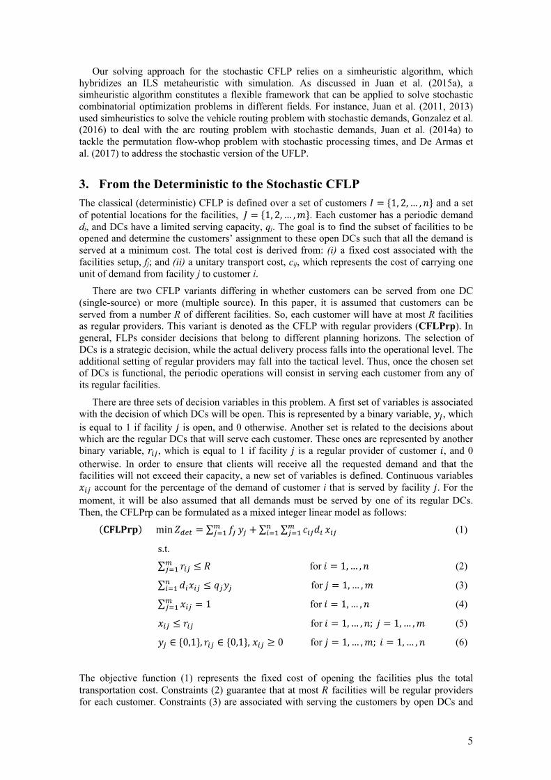
3. From the Deterministic to the Stochastic CFLP The classical (deterministic) CFLP is defined over a set of customers 𝐼 = {1, 2, … , 𝑛} and a set of potential locations for the facilities, 𝐽 = {1, 2, … ,𝑚}. Each customer has a periodic demand di, and DCs have a limited serving capacity, qj. The goal is to find the subset of facilities to be opened and determine the customers’ assignment to these open DCs such that all the demand is served at a minimum cost. The total cost is derived from: (i) a fixed cost associated with the facilities setup, fj; and (ii) a unitary transport cost, cij, which represents the cost of carrying one unit of demand from facility j to customer i.

There are two CFLP variants differing in whether customers can be served from one DC (single-source) or more (multiple source). In this paper, it is assumed that customers can be served from a number R of different facilities. So, each customer will have at most R facilities as regular providers. This variant is denoted as the CFLP with regular providers (CFLPrp). In general, FLPs consider decisions that belong to different planning horizons. The selection of DCs is a strategic decision, while the actual delivery process falls into the operational level. The additional setting of regular providers may fall into the tactical level. Thus, once the chosen set of DCs is functional, the periodic operations will consist in serving each customer from any of its regular facilities.

There are three sets of decision variables in this problem. A first set of variables is associated with the decision of which DCs will be open. This is represented by a binary variable, 𝑦!, which is equal to 1 if facility 𝑗 is open, and 0 otherwise. Another set is related to the decisions about which are the regular DCs that will serve each customer. These ones are represented by another binary variable, 𝑟"!, which is equal to 1 if facility 𝑗 is a regular provider of customer 𝑖, and 0 otherwise. In order to ensure that clients will receive all the requested demand and that the facilities will not exceed their capacity, a new set of variables is defined. Continuous variables 𝑥"! account for the percentage of the demand of customer i that is served by facility 𝑗. For the moment, it will be also assumed that all demands must be served by one of its regular DCs. Then, the CFLPrp can be formulated as a mixed integer linear model as follows:

(𝐂𝐅𝐋𝐏𝐫𝐩)min 𝑍#$% = ∑ 𝑓!&!'( 𝑦! +∑ ∑ 𝑐"!𝑑"&

!'()"'( 𝑥"! (1)

s.t. ∑ 𝑟"!&!'( ≤ 𝑅for𝑖 = 1,… , 𝑛 (2)

∑ 𝑑"𝑥"!)"'( ≤ 𝑞!𝑦! for𝑗 = 1,… ,𝑚 (3)

∑ 𝑥"!&!'( = 1for𝑖 = 1,… , 𝑛 (4)

𝑥"! ≤ 𝑟"! for𝑖 = 1,… , 𝑛; 𝑗 = 1,… ,𝑚 (5)

𝑦! ∈ {0,1}, 𝑟"! ∈ {0,1}, 𝑥"! ≥ 0for 𝑗 = 1,… ,𝑚; 𝑖 = 1,… , 𝑛 (6)

The objective function (1) represents the fixed cost of opening the facilities plus the total transportation cost. Constraints (2) guarantee that at most 𝑅 facilities will be regular providers for each customer. Constraints (3) are associated with serving the customers by open DCs and

6

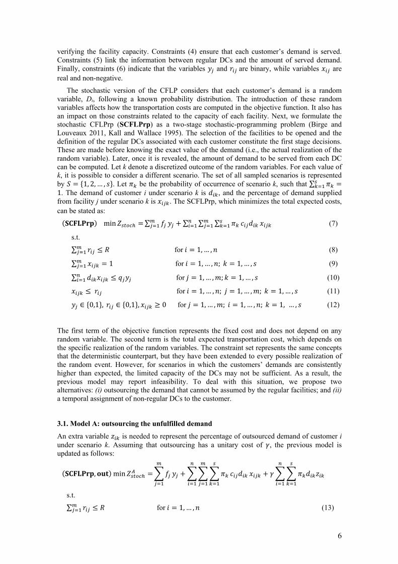
verifying the facility capacity. Constraints (4) ensure that each customer’s demand is served. Constraints (5) link the information between regular DCs and the amount of served demand. Finally, constraints (6) indicate that the variables 𝑦! and 𝑟"! are binary, while variables 𝑥"! are real and non-negative.

The stochastic version of the CFLP considers that each customer’s demand is a random variable, Di, following a known probability distribution. The introduction of these random variables affects how the transportation costs are computed in the objective function. It also has an impact on those constraints related to the capacity of each facility. Next, we formulate the stochastic CFLPrp (SCFLPrp) as a two-stage stochastic-programming problem (Birge and Louveaux 2011, Kall and Wallace 1995). The selection of the facilities to be opened and the definition of the regular DCs associated with each customer constitute the first stage decisions. These are made before knowing the exact value of the demand (i.e., the actual realization of the random variable). Later, once it is revealed, the amount of demand to be served from each DC can be computed. Let k denote a discretized outcome of the random variables. For each value of k, it is possible to consider a different scenario. The set of all sampled scenarios is represented by 𝑆 = {1, 2, … , 𝑠}. Let 𝜋* be the probability of occurrence of scenario k, such that ∑ 𝜋*+

*'( =1. The demand of customer i under scenario k is 𝑑"*, and the percentage of demand supplied from facility j under scenario k is 𝑥"!*. The SCFLPrp, which minimizes the total expected costs, can be stated as: (𝐒𝐂𝐅𝐋𝐏𝐫𝐩)min 𝑍+%,-. =∑ 𝑓!&

!'( 𝑦! + ∑ ∑ ∑ 𝜋*+*'( 𝑐"!𝑑"*&

!'( 𝑥"!*)"'( (7)

s.t. ∑ 𝑟"!&!'( ≤ 𝑅for𝑖 = 1,… , 𝑛 (8)

∑ 𝑥"!*&!'( = 1 for𝑖 = 1,… , 𝑛; 𝑘 = 1,… , 𝑠 (9)

∑ 𝑑"*𝑥"!*)"'( ≤ 𝑞!𝑦! for𝑗 = 1,… ,𝑚; 𝑘 = 1,… , 𝑠 (10)

𝑥"!* ≤𝑟"! for𝑖 = 1,… , 𝑛; 𝑗 = 1,… ,𝑚; 𝑘 = 1,… , 𝑠 (11)

𝑦! ∈ {0,1}, 𝑟"! ∈ {0,1}, 𝑥"!* ≥ 0for 𝑗 = 1,… ,𝑚; 𝑖 = 1,… , 𝑛; 𝑘 = 1, … , 𝑠 (12)

The first term of the objective function represents the fixed cost and does not depend on any random variable. The second term is the total expected transportation cost, which depends on the specific realization of the random variables. The constraint set represents the same concepts that the deterministic counterpart, but they have been extended to every possible realization of the random event. However, for scenarios in which the customers’ demands are consistently higher than expected, the limited capacity of the DCs may not be sufficient. As a result, the previous model may report infeasibility. To deal with this situation, we propose two alternatives: (i) outsourcing the demand that cannot be assumed by the regular facilities; and (ii) a temporal assignment of non-regular DCs to the customer.

3.1. Model A: outsourcing the unfulfilled demand

An extra variable 𝑧"* is needed to represent the percentage of outsourced demand of customer i under scenario k. Assuming that outsourcing has a unitary cost of 𝛾, the previous model is updated as follows:

(𝐒𝐂𝐅𝐋𝐏𝐫𝐩, 𝐨𝐮𝐭)min 𝑍+%,-./ =T𝑓!

&

!'(

𝑦! +TTT𝜋*

+

*'(

𝑐"!𝑑"*

&

!'(

𝑥"!*

)

"'(

+ 𝛾TT𝜋*𝑑"*𝑧"*

+

*'(

)

"'(

s.t. ∑ 𝑟"!&!'( ≤ 𝑅for𝑖 = 1,… , 𝑛 (13)

7

∑ 𝑥"!*&!'( +𝑧"* = 1 for𝑖 = 1,… , 𝑛; 𝑘 = 1,… , 𝑠 (14)

∑ 𝑑"*𝑥"!*)"'( ≤ 𝑞!𝑦! for𝑗 = 1,… ,𝑚; 𝑘 = 1,… , 𝑠 (15)

𝑥"!* ≤𝑟"! for𝑖 = 1,… , 𝑛; 𝑗 = 1,… ,𝑚; 𝑘 = 1,… , 𝑠 (16)

𝑦! ∈ {0,1}, 𝑟"! ∈ {0,1}, 𝑥"!* ≥ 0, 𝑧"* ≥ 0for 𝑗 = 1,… ,𝑚; 𝑖 = 1,… , 𝑛; 𝑘 = 1,… , 𝑠 (17)

Note that the objective function is composed of three terms: the fixed cost of opening facilities, the expected cost of serving the customers from the regular DCs, and the expected cost of outsourcing part of the demand. The sum of the last two terms constitutes the variable cost.

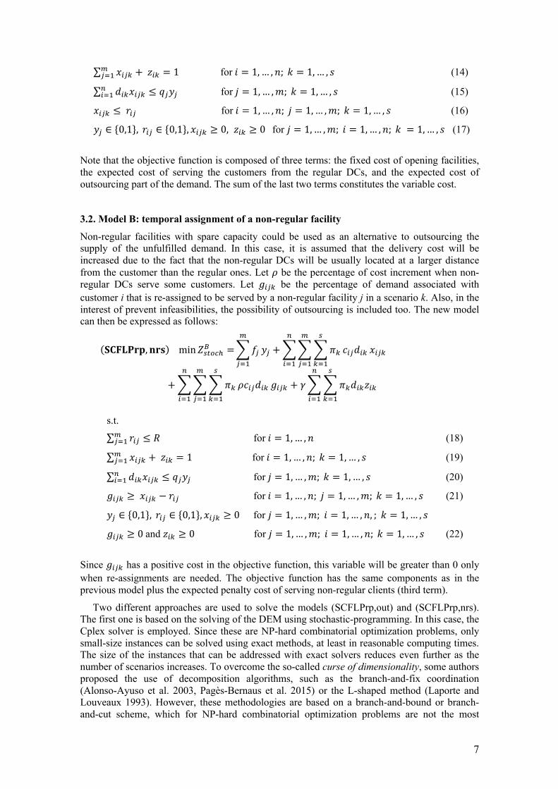
3.2. Model B: temporal assignment of a non-regular facility

Non-regular facilities with spare capacity could be used as an alternative to outsourcing the supply of the unfulfilled demand. In this case, it is assumed that the delivery cost will be increased due to the fact that the non-regular DCs will be usually located at a larger distance from the customer than the regular ones. Let 𝜌 be the percentage of cost increment when non-regular DCs serve some customers. Let 𝑔"!* be the percentage of demand associated with customer i that is re-assigned to be served by a non-regular facility j in a scenario k. Also, in the interest of prevent infeasibilities, the possibility of outsourcing is included too. The new model can then be expressed as follows:

(𝐒𝐂𝐅𝐋𝐏𝐫𝐩, 𝐧𝐫𝐬)min 𝑍+%,-.0 =T𝑓!

&

!'(

𝑦! +TTT𝜋*

+

*'(

𝑐"!𝑑"*

&

!'(

𝑥"!*

)

"'(

+TTT𝜋*

+

*'(

𝜌𝑐"!𝑑"*

&

!'(

𝑔"!*

)

"'(

+ 𝛾TT𝜋*𝑑"*𝑧"*

+

*'(

)

"'(

s.t. ∑ 𝑟"!&!'( ≤ 𝑅for𝑖 = 1,… , 𝑛 (18)

∑ 𝑥"!*&!'( +𝑧"* = 1 for𝑖 = 1,… , 𝑛; 𝑘 = 1,… , 𝑠 (19)

∑ 𝑑"*𝑥"!*)"'( ≤ 𝑞!𝑦! for𝑗 = 1,… ,𝑚; 𝑘 = 1,… , 𝑠 (20)

𝑔"!* ≥𝑥"!* − 𝑟"! for𝑖 = 1,… , 𝑛; 𝑗 = 1,… ,𝑚; 𝑘 = 1,… , 𝑠 (21)

𝑦! ∈ {0,1}, 𝑟"! ∈ {0,1}, 𝑥"!* ≥ 0for 𝑗 = 1,… ,𝑚; 𝑖 = 1,… , 𝑛, ; 𝑘 = 1,… , 𝑠

𝑔"!* ≥ 0and 𝑧"* ≥ 0for 𝑗 = 1,… ,𝑚; 𝑖 = 1,… , 𝑛; 𝑘 = 1,… , 𝑠 (22)

Since 𝑔"!* has a positive cost in the objective function, this variable will be greater than 0 only when re-assignments are needed. The objective function has the same components as in the previous model plus the expected penalty cost of serving non-regular clients (third term).

Two different approaches are used to solve the models (SCFLPrp,out) and (SCFLPrp,nrs). The first one is based on the solving of the DEM using stochastic-programming. In this case, the Cplex solver is employed. Since these are NP-hard combinatorial optimization problems, only small-size instances can be solved using exact methods, at least in reasonable computing times. The size of the instances that can be addressed with exact solvers reduces even further as the number of scenarios increases. To overcome the so-called curse of dimensionality, some authors proposed the use of decomposition algorithms, such as the branch-and-fix coordination (Alonso-Ayuso et al. 2003, Pagès-Bernaus et al. 2015) or the L-shaped method (Laporte and Louveaux 1993). However, these methodologies are based on a branch-and-bound or branch-and-cut scheme, which for NP-hard combinatorial optimization problems are not the most

8

appropriate techniques. As the computational experiments will show, exact solvers such as Cplex can only be efficiently employed in small instances of this problem. Thus, the use of a heuristic-based solving method becomes necessary.

4. Our Simheuristic Approach for the Stochastic CFLP As explained in the Introduction, our simheuristic algorithm relies on the well-known ILS metaheuristic framework. A well-designed ILS algorithm has all the desirable attributes of a metaheuristic according to Cordeau et al. (2002): accuracy, speed, simplicity, and flexibility. In Grasas et al. (2016), the authors propose the SimILS simheuristic framework, which is an extension of the ILS metaheuristic aimed at solving stochastic combinatorial optimization problems. The main idea consists in integrating a simulation component after the local search stage to evaluate the newly generated solution and provide valuable feedback. This feedback can then be used to update the base solution –i.e., to guide the search process inside the metaheuristic. This simulation component takes the new solution and a parameter indicating the number of simulation runs to be executed. In return, it provides a sample of observations on the performance of the new solution in a stochastic environment. From these observations, it becomes straightforward to obtain sample statistics such as the expected cost of the new solution, its variance, quartiles, etc. It also allows checking probabilistic constraints in case they exist –e.g., a constraint requiring that the percentage of customers requiring outsourcing or service from non-regular facilities falls below a given threshold.

In the SCFLPrp, the stochasticity is associated with the constraints and with the objective function. In both models, the possibility of outsourcing guarantees the existence of at least one feasible solution, although some solutions may have an extremely high cost. Notice that there are three decisions to make in the SCFLPrp: (a) which DCs should be opened; (b) which facilities will regularly serve each customer; and (c) the actual percentage of the demand served by each provider (regular DCs, non-regular ones, or external companies in the case of outsourcing). The two first decisions are strategic, and they should not be changed on the short run. However, the last one can vary on the short run depending on fluctuations in customers’ demands. These three decisions are set in successive steps. Algorithm 1 provides an overview of our SimILS approach. The local search stage focuses on providing configurations of open/closed facilities, as well as on the selection of the regular DCs. In the simulation stage, customers’ assignment decisions are made. Since the simulation stage is time consuming, only ‘promising’ solutions are tested in a stochastic environment. The way a local solution is labeled as promising is based on its deterministic cost. Thus, when a new solution improves the incumbent one in deterministic cost, it is considered as a promising solution and enters the simulation stage. Once the metaheuristic search is finished, a more computationally-intensive simulation stage can be added to increase the accuracy of the estimated values. At some steps of the solving process we make use of exact methods, and thus the algorithm could be considered as a matheuristic one (Lagos et al. 2016).

Procedure SimILS(inputData) 01 initSol ß generateInitialSolution(inputData) 02 03

baseSol ß localSearch(initSol) avgCost(baseSol) ß shortSimulation(baseSol)

04 bestSol ß baseSol 05 Repeat 06 newSol ß perturbation(baseSol) 07 newSol ß localSearch(newSol) 08 isPromising ß acceptanceCriterion(baseSol, newSol) 09 If (isPromising) Then 10 avgCost(newSol) ß shortSimulation(newSol) 11 12 13 14 15

If (avgCost(newSol) <= avgCost(baseSol)) Then baseSol ß newSol % baseSol is simulation-driven If (avgCost(newSol) < avgCost(bestSol)) Then bestSol ß newSol End If

9

16 End If 17 End If 18 Until (termination condition is met) 19 avgCost(bestSol) ß longSimulation(bestSol) 20 Return (bestSol)

Algorithm 1. Overview of the SimILS algorithm for the SCFLPrp

Algorithm 2 describes how the initial solution is generated. Using the deterministic scenario, a subset of open DCs is chosen randomly, but ensuring that the total capacity is higher than the total expected demand. Afterwards, employing expected demands as the only scenario and fixing variables𝑦!, model (SCFLPrp, out) or (SCFLPrp, nrs) is solved using Cplex. Thus, the following outcomes are obtained: (a) the regular facilities for each customer (variables 𝑟"!); (b) the percentage served by regular DCs (variables 𝑥"!) and by non-regular facilities (variables 𝑔"!); and (c) the amount of delivery that is outsourced.

Procedure generateInitialSolution(inputData) 01 totalDemand ß getTotalCustomersDemand(inputData) 02 facilsList ß getListOfFacilities(inputData) 03 openFacils ß empty 04 While (totalCapacity(openFacils) < totalDemand) do 05 newFacil ß randomSelect(facilsList) 06 openFacils ß addFacility(openFacils, newFacil) 07 End While 08 Set up model (CFLPrp, out/nrs) with openFacils 09 initSol ß solveExact(CFLPrp,out/nrs) 10 Return initSol

Algorithm 2. Procedure to generate an initial solution The aim of the perturbation procedure is to produce a new map of open DCs each time it is called. In this way, the risk of being trapped in a local minimum is noticeably reduced. The map re-generation is achieved by a classical destruction-and-reconstruction process, i.e.: a random selection of the DCs in the current base solution are closed and, in turn, new randomly chosen facilities are opened. Thus, this new map of open facilities is not constructed from scratch, but it maintains part of the DNA of the base solution –which, as the algorithm evolves, tends to be a better solution for the stochastic version of the problem.

Finally, a local search procedure is applied to improve any newly generated solution. It is based on operators that change the set of open DCs. Specifically, three operators are used: (a) open new facilities from the set of closed ones; (b) close some of the open DCs; and (c) swap a closed facility with an open one. The local search iterates for a predefined number of trials (100 in our case). After the local search stage, the set of DCs to open and the set of regular providers for each customer are fixed. This solution needs to be tested in a stochastic environment to assess its performance.

5. Computational Experiments This Section includes a series of computational experiments aimed at: (i) illustrating the advantages of using a simulation-optimization solving approach when dealing with stochastic optimization problems; and (ii) showing the difficulty of solving the problem addressed in this paper using standard exact methods alone. For each considered instance, we have tried to solve its deterministic equivalent model using a scenario tree. The main advantage of this methodology is that optimal solutions can potentially be found with complete information (or at least as much as the scenario tree captures) of the variability structure. However, the number of variables and constraints grows proportionally to the number of scenarios, which sometimes

10

results in models that are far too large to be solved using this approach. As it will be properly discussed, in those cases our SimILS algorithm will show to be a valid alternative.

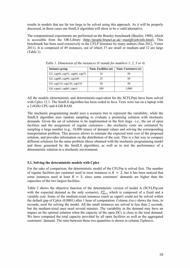
The computational experiments are performed on the Beasley benchmark (Beasley 1988), which is accessible from the OR-Library (http://people.brunel.ac.uk/~mastjjb/jeb/info.html). This benchmark has been used extensively in the CFLP literature by many authors (Sun 2012, Verter 2011). It is composed of 49 instances, out of which 37 are small or medium and 12 are large (Table 1).

Table 1. Dimension of the instances (# stands for numbers 1, 2, 3 or 4)

Instance group Num. Facilities (m) Num. Customers (n)

G1: cap4#, cap51, cap6#, cap7# 16 50

G2: cap8#, cap9#, cap10# 25 50

G3: cap11#, cap12#, cap13# 50 50

G4: capa#, capb#, capc# 100 1,000

All the models (deterministic and deterministic-equivalent for the SCFLPrp) have been solved with Cplex 12.1. The SimILS algorithm has been coded in Java. Tests were run on a laptop with a 2.6GHz CPU and 4 GB RAM.

The stochastic programming model uses a scenario tree to represent the variability, while the SimILS algorithm uses random sampling to evaluate a promising solution with stochastic demands. Given the set of solutions to be implemented in the first stage –i.e., the set of open facilities and the assignment of regular customers–, the stochastic costs are estimated by sampling a large number (e.g., 10,000 times) of demand values and solving the corresponding transportation problem. This process allows to estimate the expected total cost of the proposed solution, and provides information on the distribution of the cost. This is a fair way to compare different solutions for the same problem (those obtained with the stochastic programming model and those generated by the SimILS algorithm), as well as to test the performance of a deterministic solution in a stochastic environment.

5.1. Solving the deterministic models with Cplex

For the sake of comparison, the deterministic model of the CFLPrp is solved first. The number of regular facilities per customer used in most instances is 𝑅 = 2, but it has been noticed that some instances need at least 𝑅 = 3, since some customers’ demands are higher than the capacities of the two largest facilities.

Table 2 shows the objective function of the deterministic version of model A (SCFLPrp,out with the expected demand as the only scenario), 𝑍#$%/ , which is composed of a fixed and a variable cost. Some of the medium-sized instances (such as capa#) could not be solved within the default gap of Cplex (0.0001) after 1 hour of computation. Column t(sec) shows the time, in seconds, used for solving the model. All the small instances are solved in less than 2 seconds, but the medium-sized ones need several minutes. The variability in the demand may have an impact on the optimal solution when the capacity of the open DCs is close to the total demand. We have computed the total capacity provided by all open facilities as well as the aggregated customers’ demand. The ratio between these two quantities is shown in column Tightness.

11

Table 2. Results for the deterministic version of model A Instance R t (sec) 𝒁𝒅𝒆𝒕𝑨 Tightness Instance R t (sec) 𝒁𝒅𝒆𝒕𝑨 Tightness cap41 3 0.14 1045083 89.6 cap111 3 0.48 826124 68.6 cap42 3 0.17 1102640 97.1 cap112 3 1.03 901376 77.7 cap43 3 0.16 1157640 97.1 cap113 3 1.16 970569 83.2 cap44 3 0.16 1240140 97.1 cap114 3 1.74 1066451 89.6 cap51 2 0.39 1025208 72.8 cap121 2 0.70 793440 25.9 cap61 2 0.17 932617 35.3 cap122 2 1.42 852525 35.3 cap62 2 0.17 977801 43.2 cap123 2 1.55 895304 43.2 cap63 2 0.38 1014063 55.5 cap124 2 1.64 946052 55.5 cap64 2 0.33 1045652 77.7 cap131 2 0.66 793440 6.7 cap71 2 0.19 932617 9.1 cap132 2 0.98 851496 9.1 cap72 2 0.16 977801 11.1 cap133 2 0.94 893079 12.5 cap73 2 0.23 1010642 20.0 cap134 2 1.34 928945 25.0 cap74 2 0.16 1034979 25.0 capa1* 2 3600.86 19242041 90.9 cap81 3 0.28 838635 68.6 capa2* 2 3601.38 18455311 84.8 cap82 3 0.41 914775 77.7 capa3* 2 3601.30 17782690 84.8 cap83 3 0.64 980343 83.2 capa4 2 455.20 17160910 90.9 cap84 3 0.56 1072713 89.6 capb1 2 474.44 13656488 93.5 cap91 2 0.23 796649 25.9 capb2 2 1211.30 13361939 95.2 cap92 2 0.64 855734 35.3 capb3 2 1058.01 13198566 91.8 cap93 2 0.75 896618 48.6 capb4 2 1337.59 13082535 91.8 cap94 2 0.94 946052 55.5 capc1 2 825.41 11646585 92.6 cap101 2 0.22 796649 6.7 capc2 2 478.89 11570336 88.6 cap102 2 0.42 854705 9.1 capc3 2 346.84 11518730 87.1 cap103 2 0.38 893783 12.5 capc4 2 409.89 11506487 78.1 cap104 2 0.33 928945 25.0 In the case of model B (deterministic version of SCFLPrp,nrs), Table 3 shows only those instances with results different from the ones obtained for model A. Notice that, for the deterministic version, only a few instances make use of re-assignments. Specifically, cap4#, cap8#, and cap11#. In addition, since model B is an extension of model A, the total cost of model B has to be equal or smaller than that of model A. The time needed for solving these instances are similar than in the case of model A.

Table 3. Solution to the deterministic model B Instance R t (sec) 𝒁𝒅𝒆𝒕𝑩 cap41 3 0.25 1043905 cap42 3 0.55 1101462 cap43 3 0.23 1156462 cap44 3 0.66 1238962 cap81 3 0.30 838635 cap82 3 0.45 912899 cap83 3 0.64 977899 cap84 3 0.42 1070263 cap111 3 0.76 826124 cap112 3 1.39 901376 cap113 3 1.45 970569 cap114 3 1.45 1064199

5.2. Solving the stochastic models

The deterministic instances have been used as the basis for the stochastic ones. Stochastic demands follow a known statistical distribution,𝐷", with a given mean and variance. Without loss of generality, we assumed that the demand of customer i follows a Log-Normal distribution with mean 𝐸(𝐷") = 𝑑" (where 𝑑" is the periodic demand of customer i in the deterministic benchmark), and standard deviation proportional to the mean value, i.e.:𝑆𝐷(𝐷") = 𝜅𝑑". Logically, as the value of 𝜅converges to zero the results from the stochastic version should converge to those obtained in the deterministic scenario. In other words, the deterministic

12

benchmark has been extended to a stochastic benchmark in a natural way. Note that the assumption on the demand distribution is made only to generate some numerical data that can be used in our experiments. Nevertheless, in a real-life application the modeler can use any other distribution based on historical data. If the inverse transform method is used to sample the Log-Normal distribution, the scaled mean 𝜇" (also called location parameter), and the standard deviation 𝜎" (or scale parameter) can be computed as follows:

𝜇" = 𝑙𝑛

⎝

⎜⎛ 1(3&)

5(6'()(&*

2

𝐸)𝐷𝑖*2⎠

⎟⎞= 𝑙𝑛 g #&

7(682h 𝜎" = i𝑙𝑛 g1 + 93(3&)2

𝐸(𝐷𝑖)2 h = jln(1 + 𝜅2)

We have tested the instances with several levels of demand variability by setting the parameter 𝜅 to different values. In particular, we used the values 𝜅 = 0.1 and 𝜅 = 0.2. For each level, Figure 2 shows the distribution of the aggregated customers’ demand for the instance cap41. Notice that, although the individual distributions are asymmetric, the sum of many values produces a quite symmetric distribution centered at the expected value.

Figure 2. Distribution of the aggregated customers’ demand (case cap41)

Regarding the specific parameters used in the stochastic version, we assumed an increased cost of re-assignment 20% higher than the regular assignment cost (𝜌 = 0.2). Likewise, we assumed a flat-rate outsourcing cost of𝛾 = 150 for the small cases, and of 𝛾 = 2,000 for the large ones. The value of 𝛾has been chosen to be higher than the 𝜌% of the highest 𝑐"! (which represents the unitary cost), so the outsourcing cost is always more expensive than serving from any in-house facility. The stochastic models have been solved using both Cplex and our SimILS approach. The model solved by Cplex is the deterministic equivalent one, using a scenario tree with 200 scenarios. The method used to build the scenario tree is a Monte Carlo sampling technique. The number of variables and the number of constraints grows proportionally to the number of scenarios considered. Fortunately, the number of binary variables remains the same as that of the deterministic model. However, this fact did not prevent the DEM to run out of memory for the larger instances (G4).

In the case of instances with large spare capacity, it is likely that deterministic solutions perform well when used in a stochastic environment. However, for tighter instances the deterministic solutions may frequently require the use of external support, which will generate a noticeable increase of the variable cost. In what follows, we focus our analysis in the subset of instances with a tightness percentage higher than 50%. Thus, Table 4 compares the solutions obtained with the two solving approaches for the model A under a variability level of 𝜅 = 0.2.

13

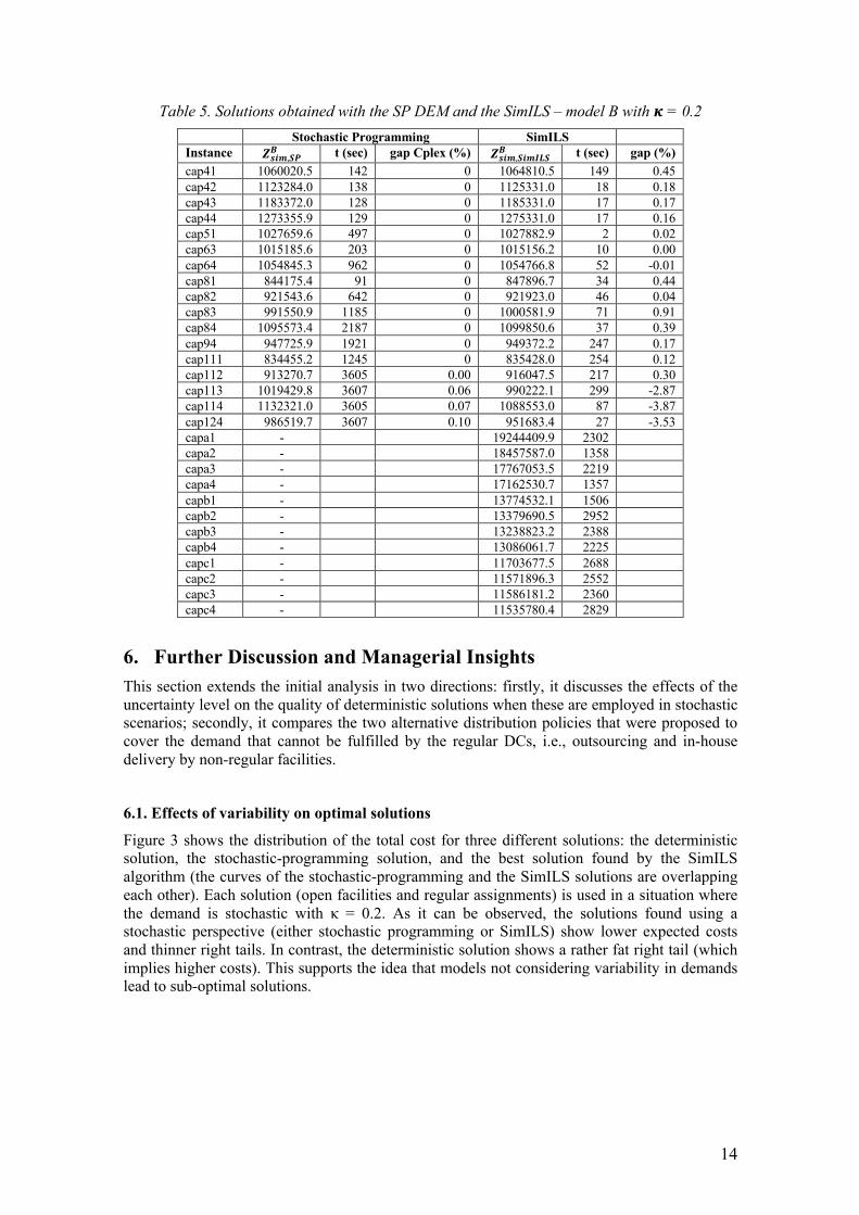
For each solution (found either by Cplex or SimILS), column 𝑍+"&,#/ shows the expected total cost. Equivalent results for model B are shown in Table 5.

Table 4. Solutions obtained with the SP DEM and the SimILS – model A with 𝜿 = 0.2

Stochastic Programming SimILS

Instance 𝒁𝒔𝒊𝒎,𝑺𝑷𝑨 t (sec) gap Cplex (%) 𝒁𝒔𝒊𝒎,𝑺𝒊𝒎𝑰𝑳𝑺𝑨 t (sec) gap (%) cap41 1099053.3 118 0 1108174.6 54 0.83 cap42 1159055.3 137 0 1161130.6 0 0.18 cap43 1219047.5 189 0 1221130.6 0 0.17 cap44 1309049.7 192 0 1311130.6 0 0.16 cap51 1029624.8 496 0 1029890.0 0 0.03 cap63 1015698.5 196 0 1015156.2 26 -0.05 cap64 1055515.6 842 0 1055271.1 25 -0.02 cap81 888939.5 155 0 890108.6 50 0.13 cap82 966076.1 768 0 969763.0 53 0.38 cap83 1036037.8 1329 0 1043960.0 26 0.76 cap84 1137068.5 3523 0 1143882.0 0 0.60 cap94 947986.3 2471 0 949375.9 5 0.15 cap111 879371.7 1103 0 883539.4 170 0.47 cap112 965382.2 3604 0.01 958047.4 303 -0.76 cap113 1047322.2 3603 0.04 1030653.5 294 -1.59 cap114 1160395.4 3604 0.06 1139246.8 50 -1.82 cap124 975397.6 3603 0.09 949375.9 65 -2.67 capa1 -

19244150.7 2263

capa2 -

18458612.4 2370

capa3 -

17827599.1 2934

capa4 -

17162132.3 963

capb1 -

13773560.0 809

capb2 -

13378972.7 2645

capb3 -

13238010.0 2086

capb4 -

13084859.8 2380

capc1 -

11704267.9 1363

capc2 -

11571933.3 1812

capc3 -

11540950.9 2850

capc4 -

11535842.8 1928

The DEM solved with Cplex is allowed to run for 1 hour. The gap column shows the goodness of the returned solution. Note that 4 instances from the G3 group cannot be solved to optimality within the given time limit. Moreover, the larger instances (G4) report an out-of-memory message without providing any feasible solution. On the contrary, the SimILS approach was given 300 seconds for finding a solution in the small-medium instances (G1, G2, and G3) and 3,000 seconds for the large instances (G4). The column t(sec) shows the time at which the best stochastic solution was found. As usual, the gaps between the solutions found by the stochastic-programming approach and our SimILS algorithm has been computed as 100 · (𝑍+"&,9"&<=9/ −𝑍+"&,9>/ )/𝑍+"&,9>/ . Comparing the small-medium instances, both approaches provide solutions of similar quality (with an average gap of -0.18% for model A and -0.41% for model B in favor of the stochastic programming approach). However, the time employed by the SimILS approach is one order of magnitude smaller. Moreover, for the larger instances G4 the SimILS increases the required computing time, but is able to provide feasible solutions. Similar conclusions can be drawn from Table 5 for model B. Both models will be further analyzed in the next section.

14

Table 5. Solutions obtained with the SP DEM and the SimILS – model B with 𝜿 = 0.2

Stochastic Programming SimILS

Instance 𝒁𝒔𝒊𝒎,𝑺𝑷𝑩 t (sec) gap Cplex (%) 𝒁𝒔𝒊𝒎,𝑺𝒊𝒎𝑰𝑳𝑺𝑩 t (sec) gap (%) cap41 1060020.5 142 0 1064810.5 149 0.45 cap42 1123284.0 138 0 1125331.0 18 0.18 cap43 1183372.0 128 0 1185331.0 17 0.17 cap44 1273355.9 129 0 1275331.0 17 0.16 cap51 1027659.6 497 0 1027882.9 2 0.02 cap63 1015185.6 203 0 1015156.2 10 0.00 cap64 1054845.3 962 0 1054766.8 52 -0.01 cap81 844175.4 91 0 847896.7 34 0.44 cap82 921543.6 642 0 921923.0 46 0.04 cap83 991550.9 1185 0 1000581.9 71 0.91 cap84 1095573.4 2187 0 1099850.6 37 0.39 cap94 947725.9 1921 0 949372.2 247 0.17 cap111 834455.2 1245 0 835428.0 254 0.12 cap112 913270.7 3605 0.00 916047.5 217 0.30 cap113 1019429.8 3607 0.06 990222.1 299 -2.87 cap114 1132321.0 3605 0.07 1088553.0 87 -3.87 cap124 986519.7 3607 0.10 951683.4 27 -3.53 capa1 -

19244409.9 2302

capa2 -

18457587.0 1358

capa3 -

17767053.5 2219

capa4 -

17162530.7 1357

capb1 -

13774532.1 1506

capb2 -

13379690.5 2952

capb3 -

13238823.2 2388

capb4 -

13086061.7 2225

capc1 -

11703677.5 2688

capc2 -

11571896.3 2552

capc3 -

11586181.2 2360

capc4 -

11535780.4 2829

6. Further Discussion and Managerial Insights This section extends the initial analysis in two directions: firstly, it discusses the effects of the uncertainty level on the quality of deterministic solutions when these are employed in stochastic scenarios; secondly, it compares the two alternative distribution policies that were proposed to cover the demand that cannot be fulfilled by the regular DCs, i.e., outsourcing and in-house delivery by non-regular facilities.

6.1. Effects of variability on optimal solutions

Figure 3 shows the distribution of the total cost for three different solutions: the deterministic solution, the stochastic-programming solution, and the best solution found by the SimILS algorithm (the curves of the stochastic-programming and the SimILS solutions are overlapping each other). Each solution (open facilities and regular assignments) is used in a situation where the demand is stochastic with κ = 0.2. As it can be observed, the solutions found using a stochastic perspective (either stochastic programming or SimILS) show lower expected costs and thinner right tails. In contrast, the deterministic solution shows a rather fat right tail (which implies higher costs). This supports the idea that models not considering variability in demands lead to sub-optimal solutions.

15

Figure 3. Cost distribution of 3 different solutions – 𝜿 = 0.2, model B, cap44

For the sake of analyzing the quality of deterministic solutions as the demand variability increases, we have estimated the total expected cost associated with the deterministic solution and the one associated with the stochastic solution. This has been performed for each level of variability, i.e.: 𝜅 = 0.1 and 𝜅 = 0.2. These estimated costs have been obtained using a simulation with 10,000 random samples of each stochastic demand. For each stochastic solution, we have computed its gap with respect to the expected cost of the deterministic solution when the latter is applied in a stochastic environment. Figure 4 displays a boxplot of these changes by variability level 𝜅, and type of solution (det for deterministic and SP for stochastic programming). Notice that, as the variability in the demand increases, using the deterministic solution instead of the stochastic one will report larger costs, while the cost associated with the stochastic solutions remains stable.

Figure 4. Variation (%) of the total expected cost as demand variability increases – model B

6.2. Comparing outsourcing vs. in-house policies

Table 6 shows aggregated results for each of the considered re-assignment models (outsourcing and in-house non-regular distribution). Notice that solutions obtained with policies based on model B show lower expected costs than solutions obtained with model A. This is reasonable since model B extends model A by adding the possibility of non-regular delivery. Based on this comparison, it is possible to estimate the savings of using re-assignments from non-regular DCs before outsourcing the demand. On the average, this policy represents around a 3% savings (of course, in a real-life application these savings will depend on the actual cost of in-house re-assignment as well as the cost of outsourcing). Notice also that both policies use the same

16

number of open facilities in all the instances except one. However, the number of regular DCs is generally lower when the assignment policy B is used. Finally, the table also shows the % of scenarios that have required outsourcing in each of the models. As it can be observed, the possibility of performing non-regular assignments absorbs nearly all the unserved demand, thus significantly reducing the need for outsourcing.

Table 6. Performance indicators of the two assignment policies Group Average gap (%)

in expected costs Difference in the total

number of assignments Outsourcing

model A Outsourcing

model B G1 1.84 6.71 11% 1%

G2 3.69 9.60 16% 0%

G3 3.76 6.20 17% 0%

G4 0.00 0.50 0% 0%

7. Conclusions and Future Work In the context of e-commerce, this paper presents two facility-location models, which consider stochastic demands as well as a restricted number of regular suppliers per customer. These models are then solved using two different approaches. On the one hand, we use a two-stage stochastic programming methodology. On the other hand, we propose a simheuristic algorithm, combining an ILS metaheuristic with simulation. According to the computational results obtained, the stochastic programming approach is efficient but limited to small- and medium-sized instances. On the contrary, the proposed simheuristic approach is able to solve large-sized instances in reasonable computing times, while providing also competitive results for smaller instances. In addition to compare both solving methodologies, the computational experiments also contribute to illustrate and quantify the effect of considering different outsourcing policies whenever the regular distribution centers cannot cover the customers’ demand, which is considered to be stochastic. To sum up, decision-makers can rely on these flexible approaches to efficiently design supply-chains. While it is clear that the simheuristic approach is needed for large-sized instances, for most of the other instances there is a trade-off between approaches’ performance in terms of computational time and solutions’ quality.

The introduction of simheuristic algorithms to analyze stochastic facility-location models is an emergent research field. In this paper we have showed its potential, but the number of different in-house/outsourcing policies and what-if scenarios that can be of interest for decision makers is almost unlimited, and a flexible tool combining the efficiency of metaheuristics with the ability of simulation to deal with uncertainty conditions can be very useful in supporting decision-makers in e-commerce business. In particular, potential lines of future research are: (a) to analyze the effect on expected costs of the maximum number of regular providers and different policies –such as using a safety stock in each facility to deal with unexpected demands; (b) to model costs as stochastic variables, since there are a number of factors with unpredictable effects on them (e.g., accidents or congestion); (c) to study heterogeneous facilities in terms of their commercial offer, which leads to demands that depend on the customers’ assignation; (d) to explore pricing strategies and replace the costs-based objective function by one focusing on benefits; and (e) to extend the models so they consider a multi-echelon supply chain.

Acknowledgments This work has been partially supported by the Spanish Ministry of Economy and Competitiveness and FEDER (TRA2013-48180-C3-P, TRA2015-71883-REDT) and the Erasmus+ programme (2016-1-ES01-KA108-023465). We also thank the support of the UOC doctoral programme.

17

References Albareda-Sambola, M., Fernández, E., Saldanha-da-Gama, F., 2011. The facility location

problem with Bernoulli demands. Omega 39, 335–345. Alonso-Ayuso, A., Escudero, L.F., Ortuño, M. T., 2003. BFC, A branch-and-fix coordination

algorithmic framework for solving some types of stochastic pure and mixed 0-1 programs. European Journal of Operational Research 151(3), 503–519.

Aydin, N., Murat, A., 2013. A swarm intelligence based sample average approximation algorithm for the capacitated reliable facility location problem. International Journal of Production Economics 145(1), 173–183.

Balinski, M.L., Spielberg, K., 1969. Methods for integer programming: Algebraic, combinatorial and enumerative. Progress in operations research 3, 195–292.

Baron, O., Berman, O., Krass, D., 2008. Facility Location with Stochastic Demand and Constraints on Waiting Time. Manufacturing & Service Operations Management 10(3), 484–505.

Beasley, J.E., 1988. An algorithm for solving large capacitated facility location problems. European Journal of Operational Research 33(3), 314–325.

Beraldi, P., Bruni, M.E., Conforti, D., 2004. Designing robust emergency medical service via stochastic programming. European Journal of Operational Research 158, 183–193.

Birge, J.R., Louveaux, F., 2011. Two-stage recourse problems. Introduction to stochastic programming, 181–263.

Carrillo, J.E., Vakharia, A.J., Wang, R., 2014. Environmental implications for online retailing. European Journal of Operational Research 239(3), 744–755.

Cordeau, J. F., Gendreau, M., Laporte, G., Potvin, J. Y., Semet, F., 2002. A guide to vehicle routing heuristics. Journal of the Operational Research Society 53, 512–522.

Criteo, 2016. What’s in and what’s out for eCommerce in 2016? Available at: http://www.criteo.com/blog/2015/12/criteo-ecommerce-industry-outlook-2016/ [Accessed April 15, 2017].

De Armas, J., Juan, A.A., Marques, J., Pedroso, J., 2017. Solving the Deterministic and Stochastic Uncapacitated Facility Location Problem: from a heuristic to a simheuristic. Journal of the Operational Research Society, DOI: 10.1057/s41274-016-0155-6.

Gessner, G.H., Snodgrass, C.R., 2015. Designing e-commerce cross-border distribution networks for small and medium-size enterprises incorporating Canadian and U.S. trade incentive programs. Research in Transportation Business and Management 16, 84–94.

Gonzalez, S., Juan, A.A., Riera, D., Elizondo, M., Ramos, J., 2016. A Simheuristic algorithm for solving the Arc Routing Problem with Stochastic Demands. Journal of Simulation, doi: 10.1057/jos.2016.11.

Grasas, A., Juan, A., Ramalhinho, H., 2016. SimILS: A Simulation-based extension of the Iterated Local Search metaheuristic for Stochastic Combinatorial Optimization. Journal of Simulation 10, 69-77.

Guignard, M., Spielberg, K., 1977. Algorithms for exploiting the structure of the simple plant location problem. Annals of Discrete Mathematics 1, 247-271.

Juan, A.A., Barrios, B., Vallada, E., Riera, D., Jorba, J., 2014a. A simheuristic algorithm for solving the permutation flow shop problem with stochastic processing times. Simulation Modelling Practice and Theory 46, 101–117.

Juan, A.A., Faulin, J., Grasman, S., Riera, D., Marull, J., Mendez, C., 2011. Using safety stocks and simulation to solve the vehicle routing problem with stochastic demands. Transportation Research Part C: Emerging Technologies 19(5), 751–765.

Juan, A.A., Faulin, J., Grasman, S.E., Rabe, M., Figueira, G., 2015a. A review of simheuristics: Extending metaheuristics to deal with stochastic combinatorial optimization problems. Operations Research Perspectives 2, 62–72.

Juan, A.A., Faulin, J., Jorba, J., Caceres, J., Marques, J., 2013. Using Parallel & Distributed Computing for Solving Real-time Vehicle Routing Problems with Stochastic Demands.

18

Annals of Operations Research 207, 43–65. Juan, A.A., Lourenço, H., Mateo, M., Luo, R., Castella, Q., 2014b. Using Iterated Local Search

for solving the Flow-Shop Problem: parametrization, randomization and parallelization issues. International Transactions in Operational Research 21(1), 103-126.

Juan, A.A., Rabe, M., Faulin, J., Grasman, S., 2015b. Simheuristics: hybridizing simulation with metaheuristics for decision-making under uncertainty. Journal of Simulation 9(4), 261–262.

Jucker, J.V., Carlson, R.C., 1976. The Simple Plant-Location Problem under Uncertainty. Operations Research 24(6), 1045–1055.

Kall, P., Wallace, S.W., 1995. Stochastic Programming. Wiley Interscience Series in Systems and Optimization.

Klose, A., Drexl, A., 2005. Facility location models for distribution system design. European Journal of Operational Research 162, 4–29.

Krarup, J., Pruzan, P. M., 1983. The simple plant location problem: survey and synthesis. European journal of operational research 12(1), 36-81.

Lagos, C., Guerrero, G., Cabrera, E., Niklander, S., Johnson, F., Paredes, F., Vega, J., 2016. A Matheuristic Approach Combining Local Search and Mathematical Programming. Scientific Programming 2016, 1.

Laporte, G., Louveaux, F. V., 1993. The integer L-shaped method for stochastic integer programs with complete recourse. Operations Research Letters 13(3), 133–142.

Laporte, G., Louveaux, F. V., van Hamme, L., 1994. Exact Solution to a Location Problem with Stochastic Demands. Transportation Science 28(2), 95–103.

Lau, H.C., Jiang, Z.Z., Ip, W.H., Wang, D., 2010. A credibility-based fuzzy location model with Hurwicz criteria for the design of distribution systems in B2C e-commerce. Computers and Industrial Engineering 59(4), 873–886.

Lin, C.K.Y., 2009. Stochastic single-source capacitated facility location model with service level requirements. International Journal of Production Economics 117, 439–451.

Lourenço, H.R., Martin, O.C., Stützle, T., 2010. Iterated Local Search: Framework and Applications. In: Handbook of Metaheuristics. pp. 363–397.

Louveaux, F. V., Peeters, D., 1992. A Dual-Based Procedure for Stochastic Facility Location. Operations Research 40(3), 564–573.

Melo, M.T., Nickel, S., Saldanha-da-gama, F., 2009. Facility location and supply chain management – A review. European Journal of Operational Research 196(2), 401–412.

Morganti, E., Seidel, S., Blanquart, C., Dablanc, L., Lenz, B., 2014. The impact of e-commerce on final deliveries: alternative parcel delivery services in France and Germany. International Scientific Conference on Mobility and Transport 4, 1–19.

Owen, S.H., Daskin, M.S., 1998. Strategic facility location: A review. European Journal of Operational Research 111, 423–447.

Pagès-Bernaus, A., Pérez-Valdés, G., Tomasgard, A., 2015. A parallelised distributed implementation of a Branch and Fix Coordination algorithm. European Journal of Operational Research 244, 77–85.

Revelle, C. S., Swain, R. W., 1970. Central facilities location. Geographical analysis 2(1), 30–42.

Revelle, C.S., Eiselt, H.A., Daskin, M.S., 2008. A bibliography for some fundamental problem categories in discrete location science. European Journal of Operational Research 184, 817–848.

Schütz, P., Stougie, L., Tomasgard, A., 2008. Stochastic facility location with general long-run costs and convex short-run costs. Computers and Operations Research 35, 2988–3000.

Siddiqui, A.W., Raza, S.A., 2015. Electronic supply chains: Status & perspective. Computers and Industrial Engineering 88, 536–556.

Snyder, L.V., 2006. Facility location under uncertainty: A review. IIE Transactions 38, 547–564.

Snyder, L.V., Daskin, M.S., Teo, C.P., 2007. The stochastic location model with risk pooling. European Journal of Operational Research 179, 1221–1238.

Statista, 2016. Online reports at the Statista portal. Available at:

19

https://www.statista.com/outlook/243/102/ecommerce/europe [Accessed April 15, 2017]. Sun, M., 2012. A tabu search heuristic procedure for the capacitated facility location problem.

Journal of Heuristics 18(1), 91–118. Verter, V., 2011. Foundations of Location Analysis. In: Eiselt, H.A., Marianov, V. (Eds.),

Foundations of Location Analysis. Springer Science Business Media, pp. 25–38. Wang, Q., Batta, R., Rump, C.M., 2002. Algorithms for a facility location problem with

stochastic customer demand and immobile servers. Annals of Operations Research 111(1–4), 17–34.

Zhang, J., Wang, X., Huang, K., 2016. Integrated on-line scheduling of order batching and delivery under B2C e-commerce. Computers and Industrial Engineering 94, 280–289.