Designing aquaponic production systems

Ragnar Ingi Danner

Faculty of Life and Environmental

Sciences

University of Iceland 2016

Ragnar Ingi Danner

90 ECTS thesis submitted in partial fulfillment of a

Magister Scientiarum degree in Biology

Advisors

Ragnheiður Inga Þórarinsdóttir

Kesara Anamthawat-Jónsson

Faculty Representative

Kesara Anamthawat-Jónsson

External Examiner:

Sveinn Aðalsteinsson

Faculty of Life and Environmental Sciences

School of Engineering and Natural Sciences

University of Iceland

Reykjavik, May 2016

Designing aquaponic production systems

90 ECTS thesis submitted in partial fulfillment of a Magister Scientiarum degree in

Biology

Copyright © 2016 Ragnar Ingi Danner

All rights reserved

Faculty of Life and Environmental Sciences

School of Engineering and Natural Sciences

University of Iceland

Sturlugata 7

101, Reykjavik

Iceland

Telephone: 525 4000

Bibliographic information:

Ragnar Ingi Danner, 2016, Designing aquaponics production systems, Master’s thesis,

Faculty of Life and Environmental Sciences, University of Iceland, pp. 59.

Printing: Háskólaprent

Reykjavik, Iceland, May 2016

Abstract

Aquaponics is a method of producing food in a sustainable manner where fish and plants

are grown together in a closed loop of nutrients. An aquaponics system is comprised of fish

rearing tanks, mechanical- and biological filtration and hydroponics units in a closed loop

of nutrients. Fish waste produces nutrients for the plants in the hydroponic unit

consequently removing nutrients from the water column to make the culture water more

suitable for fish. The purpose of this research was to evaluate and calculate the production

of tilapia and different aquaponic vegetables through a study period of two years. The

suitability of locally available feed and the selection of plant species were assessed. Effects

of water flow on plant growth and nutrient utilization were measured. In this study, six

aquaponics systems were built in four different places. One of the systems was a nutrient

film technology system whereas four were deep water cultures. Moreover, a flood and

drain system was built and tested. One system was built within an industrial building and

received artificial lighting while the others were all located inside greenhouses. Tilapia,

which is one of the most popular fish in aquaculture, was reared in all systems while

different leafy green and fruiting plants were grown. The fish were fed commercial

aquaculture feed for cod and charr. The feed conversion ratio is used to assess how

effective the fish’s growth is, typical FCR for tilapia is between 1.0 and 1.8 depending on

the feed quality and environment. The FCR observed in this research was between 0.9 and

1.5. Leafy green plants especially pak-choi showed similar yield to other research,

expected approximately four times the production of fish in mature systems. Fruiting

plants did not do as well as leafy greens in this experiment.

Útdráttur

Samrækt er sjálfbær ræktunaraðferð þar sem fiskur og grænmeti er ræktað saman í lokaðri

hringrás næringarefna. Samræktarkerfi samanstendur af fiskitönkum, fastefnasíu, lífhreinsi

og vatnsræktarkerfi. Úrgangur fisksins losar næringarefni sem plönturnar nýta sér til

vaxtar, við það lækkar styrkur næringarefnanna og kerfið verður vistlegra fyrir fiskinn.

Tilgangur rannsóknarinnar var að bera saman ræktun á mismunandi tegundum grænmetis,

meta hentugleika íslensks fiskeldisfóðurs til ræktunar á beitarfiski og meta hvaða plöntur

henta best í framleiðslu með samrækt. Sex mismunandi kerfi voru byggð í rannsókninni og

mælingar framkvæmdar á þeim til að meta samspil þátta innan kerfisins og áhrif þeirra á

stöðu kerfisins. Eitt kerfið var NFT kerfi, fjögur voru svokölluð DWC kerfi og eitt var

flood and drain kerfi. Eitt DWC kerfið var byggt í iðnaðarhúsnæði, þar sem notast var við

raflýsingu. Tilapia eða beitarfiskur er einn vinsælasti eldisfiskur í heimi og var ræktaður í

öllum kerfum á meðan plöntuval var misjafnt milli kerfa og samanstóð bæði af

blaðgrænmeti sem og ávaxtaplöntum. Fiskarnir voru fóðraðir á eldisfóðri fyrir sjófisk og

bleikju og fóðurstuðull þeirra reiknaður. Fóðurstuðull er mælikvarði á hversu vel fiskurinn

vex og er jafnan á bilinu 1,0 og 1,8 fyrir beitarfisk. Í þessari rannsókn var fóðurstuðullinn á

bilinu 0,9 til 1.5. Blaðgrænmeti, sérstaklega pak-choi skilaði góðum niðurstöðum í

kerfunum, sambærilegum við aðrar rannsóknir. Ávaxtaplöntur skiluðu ekki eins góðum

árangri.

vii

Table of Contents

List of Figures ................................................................................................................... viii

List of Tables ........................................................................................................................ x

List of Equations ................................................................................................................. xi

Abbreviations ..................................................................................................................... xii

Acknowledgements ........................................................................................................... xiii

1 Introduction ..................................................................................................................... 1

2 Background ..................................................................................................................... 3 2.1 Aquaponics .............................................................................................................. 3

2.2 Nitrification ............................................................................................................. 4 2.3 Hydroponic system types ........................................................................................ 6 2.4 Fauna & Flora .......................................................................................................... 7

3 Materials and methods ................................................................................................. 11 3.1 Systems .................................................................................................................. 11

3.1.1 System 1: Show case setup ......................................................................... 11

3.1.2 System 2 – 4: Greenhouse setup .................................................................. 13

3.1.3 System 5: Industry building setup................................................................ 15

3.1.4 System 6: Commercial Pilot setup ............................................................... 17 3.2 Fauna ..................................................................................................................... 18 3.3 Flora....................................................................................................................... 18

3.4 Lighting and electrical appliances ......................................................................... 19 3.5 Statistical analysis ................................................................................................. 19

3.6 Water sampling and Chemical analysis ................................................................. 20

4 Results ............................................................................................................................ 21 4.1 System 1 ................................................................................................................ 21 4.2 Systems 2-4 ........................................................................................................... 21

4.3 System 5 ................................................................................................................ 25 4.4 System 6 ................................................................................................................ 33

5 Discussion ...................................................................................................................... 37

6 Conclusions and recommendations. ............................................................................ 41

References........................................................................................................................... 43

Appendix A feed and additive ingredients ...................................................................... 47

Appendix B Posters and other material .......................................................................... 51

Appendix C Test kit user manuals. .................................................................................. 57

viii

List of Figures

Figure 2.1 Typical setup of an aquaponic system modified from Thorarinsdottir, et al.

2015. ................................................................................................................... 4

Figure 2.2 An illustration of a decoupled aquaponic system, modified from

Thorarinsdottir et al. 2015. ................................................................................. 7

Figure 3.1 A schematic illustration of the showcase system. .............................................. 12

Figure 3.2 A photograph of System 1. ................................................................................ 12

Figure 3.3 System 2, the arrows indicate the flow of water through the system. ............... 13

Figure 3.4 A photograph taken of System 3 while it was operative, system 1 can be

seen in the background. .................................................................................... 14

Figure 3.5 System 3, the arrows indicate the flow of water through the system. ............... 14

Figure 3.6 Schematic overview of System 4. ...................................................................... 15

Figure 3.7 The layout of System 5. ..................................................................................... 16

Figure 3.8 A schematic overview System 6. Arrows indicate the course of water

through the system 1A-1C are fish tanks. 2A is the drumfilter, 2B is the

solids collection tank. 3 is the sump 4A is the biofilter, 4B is the trickling

tower and 5 is the hydroponic unit. .................................................................. 17

Figure 3.9 The hydroponic part of the system. ................................................................... 18

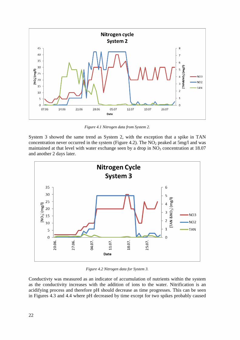
Figure 4.1 Nitrogen data from System 2. ............................................................................ 22

Figure 4.2 Nitrogen data for System 3. ............................................................................... 22

Figure 4.3 pH and conductivity data for System 2. ............................................................. 23

Figure 4.4 pH and conductivity data for System 3 in the greenhouse. ............................... 23

Figure 4.5 Basil (near) and mint (far) in System 3. ............................................................. 24

Figure 4.6 Rucola plant shows deficiency symptoms, healthy basil plant in the back. ...... 24

Figure 4.7 Tomato plants in the growbed in System 4. ....................................................... 25

Figure 4.8 Peppers in System 4. .......................................................................................... 25

ix

Figure 4.9 A graph showing the mass of edible greens produced in each bed between

runs. .................................................................................................................. 26

Figure 4.10 Nutrient concentrations in Pair A in Trial 1. .................................................... 27

Figure 4.11 Nutrient concentrations in Pair B in Trial 1. .................................................... 28

Figure 4.12 Nutrient concentrations in Pair C in Trial 1. ................................................... 28

Figure 4.13 Conductivity (EC) TDS and pH for the system in Trial 1. .............................. 29

Figure 4.14 Photos of bed B1 taken 9 days in between showing rapid growth in pak-

choi. .................................................................................................................. 29

Figure 4.15 Nutrient concentration in Pair A in Trial 2. ..................................................... 30

Figure 4.16 Nutrient concentrations in Pair B in Trial 2. .................................................... 30

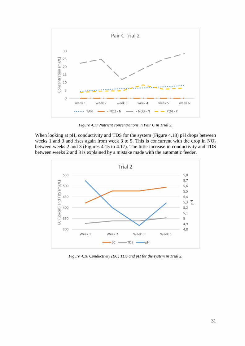
Figure 4.17 Nutrient concentrations in Pair C in Trial 2. .................................................... 31

Figure 4.18 Conductivity (EC) TDS and pH for the system in Trial 2. .............................. 31

Figure 4.19 Beds in Trial 1 at the day of harvest. ............................................................... 32

Figure 4.20 Tomato plants in System 6, bearing many fruit. .............................................. 34

Figure 4.21 Okra plants in System 6. A seed pod and a flower can bee seen at center-

left of the image. ............................................................................................... 35

x

List of Tables

Table 2.1 Different kinds of plants grown in aquaponics. .................................................... 8

Table 3.1 Systems and system types in the research. .......................................................... 11

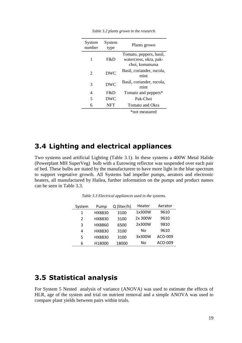
Table 3.2 plants grown in the research. ............................................................................... 19

Table 3.3 Electrical appliances used in the systems. ........................................................... 19

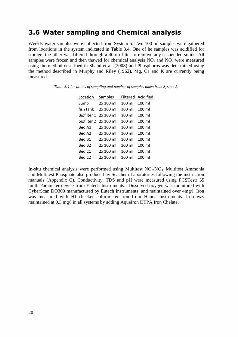
Table 3.4 Locations of sampling and number of samples taken from System 5. ................ 20

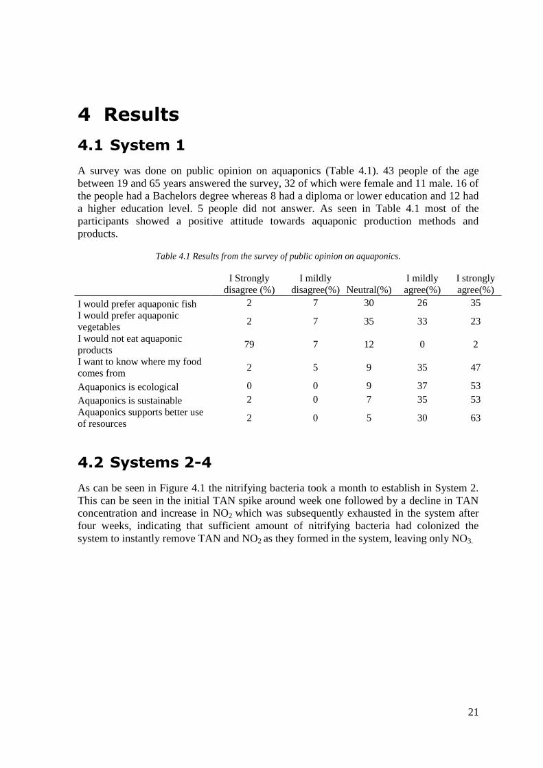
Table 4.1 Results from the survey of public opinion on aquaponics. ................................. 21

Table 4.2 Growth of fish and vegetables in the greenhouse systems. ................................ 23

Table 4.3 FCR and total plant to feed conversion ratio for the trials. ................................. 26

Table 4.4 Hydraulic loading rate (HLR) for each pair of beds. .......................................... 26

Table 4.5 Results of ANOVA for plant yield between pairs in Trial 1. .............................. 27

Table 4.6 Results of ANOVA for plant yield between pairs in Trial 2. .............................. 27

Table 4.7 Results of Nested ANOVA for effects of trials, weeks or HLR on TAN

removal. ............................................................................................................ 32

Table 4.8 Results of Nested ANOVA for effects of trials, weeks or HLR on NO2 –N

removal. ............................................................................................................ 32

Table 4.9 Results of Nested ANOVA for effects of trials, weeks or HLR on NO3–N

removal. ............................................................................................................ 32

Table 4.10 Results of Nested ANOVA for effects of trials, weeks or HLR on PO4–P

removal. ............................................................................................................ 33

Table 4.11 Growth of fish in System 6. .............................................................................. 33

Table 4.12 An explanation of plant biomass for System 6. ................................................ 33

Table 4.13 EROI results for the first 10 years of systems compared (Atlason et al.,

n.d. Table 2 included with authors permission). .............................................. 33

xi

List of Equations

Equation 1 The nitritation process (Sultana, 2014) ............................................................... 5

Equation 2 The process of nitratation (Sultana, 2014) .......................................................... 5

xii

Abbreviations

ANOVA – Analysis of variance

DWC – Deep Water Culture

FAO - Food and Agricultural Organization of the United Nations

FCR – Feed Conversion Ratio

F&D – Flood-and-drain

HLR – Hydraulic Loading Rate

MBB – Moving Bed Biofilter

NFT – Nutrient film Technique

RAS – Recirculating Aquaculture System

TAN – Total Ammonia Nitrogen

xiii

Acknowledgements

First I want to thank The University of Iceland, Svinna Engineering, Rannís and the

Ecoponics project for funding the research. Landsbankinn and the Organic farm Akur

receive gratitude for providing housing for the systems. And the following people for their

part in making this happen; Svanhvít Viðarsdóttir and Marvin Ingi Einarsson for their part

in building the systems and assisting with measurements. Ísak M. Jóhannesson, Ólafur P.

Pálsson, Rúnar Unnþórsson and Soffía K. Magnúsdóttir for their assistance with

measurements. Hermann D. Guls for assisting me with statistical analysis. Utra

Mankasingh for invaluable help with laboratory analysis. I also want to thank my advisors,

Ragnheiður Þórarinsdóttir and Kesara Anamthawat-Jónsson for their guidance and for

giving their time to make this project come true and last but not least I want to thank

Snæfríður Pétursdóttir for moral support during the stressful times of putting all of this

together.

1

1 Introduction

Aquaponics is a developing sustainable food production method coupling aquaculture and

horticulture together in one circular system mimicking nutrient and water cycles from

nature. Aquaponics has gained increased interest in recent years and the number of

aquaponic practicioners has increased greatly since 2007 (Love et al., 2014). Most

aquaponic practicioners are hobbyist mostly interested in making their own food and in

environmental issues (Love et al., 2014). However, a few startup companies in Europe

have taken the step towards commercial production (Thorarinsdottir et al., 2015). By using

renewable energy sources and abundant clean water in Iceland, aquaponic production

could develop into commercial scale production being environmentally friendly as waste

from the aquaculture and fertilizer use is minimized in aquaponics.

This study was done in cooperation with Svinna Engineering Ltd. as background studies

for establishing commercial scale aquaponic production in Iceland. The main goals of this

research were to evaluate and calculate the optimal production of different aquaponic

vegetables in different production systems and troubleshooting their design through a study

period of two years. The suitability of locally available feed for rearing tilapia was

evaluated as no special tilapia feed is produced in Iceland, and emphasis was put on

selecting suitable plant species for the production. Also the effects of water flow on plant

growth and nutrient utilization were measured, hypothesizing that plants in slower flow

would show increased growth and more nutrient removal.

The thesis is divided into five chapters. Chapter 1 is this introduction, Chapter 2 covers the

present knowledge within aquaponics and the results from other related studies. Chapter 3

presents the materials and methods used in the study, where system design, fauna and flora

of the systems, chemical and statistical analyses are described. Chapter 4 presents the

results from the experiments followed by the discussion in Chapter 5. Finally Chapter 6

contains the conclusions made from the experimental work and recommendations

regarding system design, feed and plant selection.

2

3

2 Background

2.1 Aquaponics

Aquaponics is a combination of recirculating aquaculture system (RAS), that is farming

fish in circulating systems, and hydroponics, that is growing plants in a solution of

nutrients and water (Rakocy, 1988). An aquaponic system consists of a fish rearing tank,

mechanical, and biological filtering, a hydroponic growbed and optionally a sump

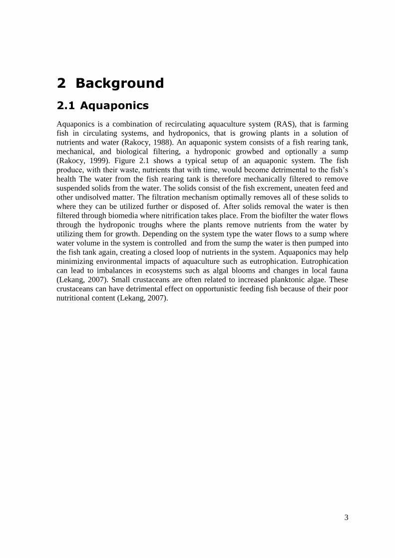
(Rakocy, 1999). Figure 2.1 shows a typical setup of an aquaponic system. The fish

produce, with their waste, nutrients that with time, would become detrimental to the fish’s

health The water from the fish rearing tank is therefore mechanically filtered to remove

suspended solids from the water. The solids consist of the fish excrement, uneaten feed and

other undisolved matter. The filtration mechanism optimally removes all of these solids to

where they can be utilized further or disposed of. After solids removal the water is then

filtered through biomedia where nitrification takes place. From the biofilter the water flows

through the hydroponic troughs where the plants remove nutrients from the water by

utilizing them for growth. Depending on the system type the water flows to a sump where

water volume in the system is controlled and from the sump the water is then pumped into

the fish tank again, creating a closed loop of nutrients in the system. Aquaponics may help

minimizing environmental impacts of aquaculture such as eutrophication. Eutrophication

can lead to imbalances in ecosystems such as algal blooms and changes in local fauna

(Lekang, 2007). Small crustaceans are often related to increased planktonic algae. These

crustaceans can have detrimental effect on opportunistic feeding fish because of their poor

nutritional content (Lekang, 2007).

4

Figure 2.1 Typical setup of an aquaponic system modified from Thorarinsdottir, et al. 2015.

After removal the solids are often composted, either as fertilizer for conventional

agriculture or mineralized in water (Lekang, 2007) where the nutrients released may be to

further use in the aquaponic system itself (Thorarinsdottir et al., 2015). It is neccessary to

remove the solids as they will adhere to plant roots (Rakocy, 1999) and could cause

negative changes to rhizosphere conditions. Accumulated solids can lead to depleted

oxygen content due to a high biochemical oxygen demand (BOD) and elevated ammonia

levels (Rakocy, 2007). BOD and chemical oxygen demand (COD) are measurements of

how much oxygen is needed to break down waste materials. As solids within a system

decompose, the bacteria consume oxygen from the water. Without removing the solids

from the system, the BOD of the system remains high, lowering oxygen concentration and

reducing the effectiveness of the biofilter (Graber et al., 2010). COD is the same as BOD

with the exception that COD includes decomposable organic matter that cannot be

decomposed with biological functions (Lekang, 2007). Mineralization is an essential

process in aquaponics. Mineralization is the process of releasing nutrients bound in solid

waste into their dissolved mineral phase.

2.2 Nitrification

Nitrification is an essential function in the system. As the fish excrete ammonia, the water

would soon become toxic without water exchange or microbial action. Nitrification is the

process of oxidizing ammonia to nitrate. Ammonia and nitrite, the first products of the

nitrification process are toxic to aquatic animals (Jensen, 2003; Kroupova et al., 2005).

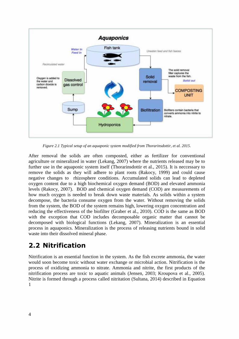
Nitrite is formed through a process called nitritation (Sultana, 2014) described in Equation

1

5

Equation 1 The nitritation process (Sultana, 2014).

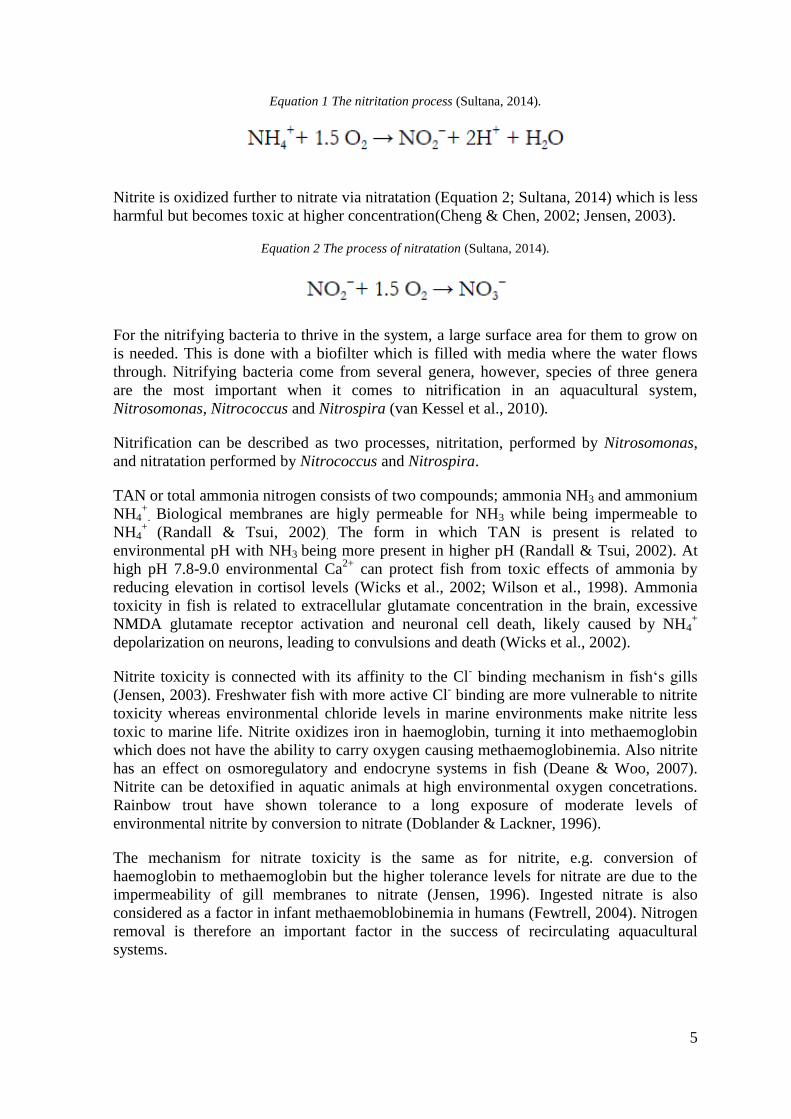
Nitrite is oxidized further to nitrate via nitratation (Equation 2; Sultana, 2014) which is less

harmful but becomes toxic at higher concentration(Cheng & Chen, 2002; Jensen, 2003).

Equation 2 The process of nitratation (Sultana, 2014).

For the nitrifying bacteria to thrive in the system, a large surface area for them to grow on

is needed. This is done with a biofilter which is filled with media where the water flows

through. Nitrifying bacteria come from several genera, however, species of three genera

are the most important when it comes to nitrification in an aquacultural system,

Nitrosomonas, Nitrococcus and Nitrospira (van Kessel et al., 2010).

Nitrification can be described as two processes, nitritation, performed by Nitrosomonas,

and nitratation performed by Nitrococcus and Nitrospira.

TAN or total ammonia nitrogen consists of two compounds; ammonia NH3 and ammonium

NH4+

. Biological membranes are higly permeable for NH3 while being impermeable to

NH4+

(Randall & Tsui, 2002). The form in which TAN is present is related to

environmental pH with NH3 being more present in higher pH (Randall & Tsui, 2002). At

high pH 7.8-9.0 environmental Ca2+

can protect fish from toxic effects of ammonia by

reducing elevation in cortisol levels (Wicks et al., 2002; Wilson et al., 1998). Ammonia

toxicity in fish is related to extracellular glutamate concentration in the brain, excessive

NMDA glutamate receptor activation and neuronal cell death, likely caused by NH4+

depolarization on neurons, leading to convulsions and death (Wicks et al., 2002).

Nitrite toxicity is connected with its affinity to the Cl- binding mechanism in fish‘s gills

(Jensen, 2003). Freshwater fish with more active Cl- binding are more vulnerable to nitrite

toxicity whereas environmental chloride levels in marine environments make nitrite less

toxic to marine life. Nitrite oxidizes iron in haemoglobin, turning it into methaemoglobin

which does not have the ability to carry oxygen causing methaemoglobinemia. Also nitrite

has an effect on osmoregulatory and endocryne systems in fish (Deane & Woo, 2007).

Nitrite can be detoxified in aquatic animals at high environmental oxygen concetrations.

Rainbow trout have shown tolerance to a long exposure of moderate levels of

environmental nitrite by conversion to nitrate (Doblander & Lackner, 1996).

The mechanism for nitrate toxicity is the same as for nitrite, e.g. conversion of

haemoglobin to methaemoglobin but the higher tolerance levels for nitrate are due to the

impermeability of gill membranes to nitrate (Jensen, 1996). Ingested nitrate is also

considered as a factor in infant methaemoblobinemia in humans (Fewtrell, 2004). Nitrogen

removal is therefore an important factor in the success of recirculating aquacultural

systems.

6

2.3 Hydroponic system types

There are various types of hydroponic system setups: Deep water culture (DWC), nutrient

film technique (NFT) and flood-and-drain (F&D) systems being the three most common

types used in aquaponics. They differ mostly in the method of irrigation.

DWC works by the plants growing in rafts floating in or being suspended over a watertight

growbed with their roots suspended in the nutrient solution that flows continuously. DWC

also adds a body of water where other organisms can be cultured. Sometimes microfauna

such as small crustaceans like ostracods and copepods, planarian flatworms and mosquito

larvae, can flourish in these conditions. Some species can be harmful to plants, but can be

remedied by introducing small predatory fish to the DWC bed (Rakocy et al., 1997).

NFT allows water to flow at a constant level through the rhizosphere of the plants, which

are grown in a vertical or horizontal tube. There is only a thin layer of nutrient solution that

continuously flows over the roots. It is essential to remove all solids in this kind of a

system as they will build up on the plant roots with detrimental causes for the plant‘s

health.

F&D systems utilize a bed of a porous medium for the plants to grow in, usually expanded

clay or pumice. The bed slowly fills up with water, when a certain maximum is reached a

simple device drains the bed for the cycle to start again. The media in the bed also serves

purposes other than just being a surface for the plant roots to stick to. The porous nature of

these materials also provides a large surface area for the essential nitrifying bacteria to

thrive on and therefore serves as a biofilter for the system, negating the need for a separate

biofilter in a well-balanced system, thus improving spatial utilization. The flushing of the

bed gives the bacteria highly oxygenated conditions that optimize their growth and

nitrification. F&D systems are however prone to solids buildup in the media. This can be

remedied by using a good solids remover or by manually removing and rinsing the media

which is labor intensive .

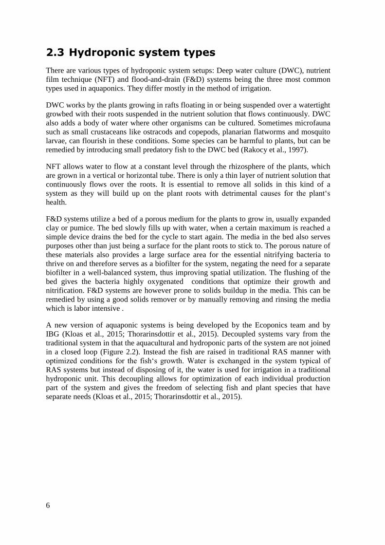
A new version of aquaponic systems is being developed by the Ecoponics team and by

IBG (Kloas et al., 2015; Thorarinsdottir et al., 2015). Decoupled systems vary from the

traditional system in that the aquacultural and hydroponic parts of the system are not joined

in a closed loop (Figure 2.2). Instead the fish are raised in traditional RAS manner with

optimized conditions for the fish‘s growth. Water is exchanged in the system typical of

RAS systems but instead of disposing of it, the water is used for irrigation in a traditional

hydroponic unit. This decoupling allows for optimization of each individual production

part of the system and gives the freedom of selecting fish and plant species that have

separate needs (Kloas et al., 2015; Thorarinsdottir et al., 2015).

7

Figure 2.2 An illustration of a decoupled aquaponic system, modified from Thorarinsdottir et al. 2015.

2.4 Fauna & Flora

Tilapia (Oreochromis niloticus) is one of the most popular fish in aquaculture and in

aquaponics systems. This is due to its omnivorous nature, rapid breeding and fast growth

which make it an ideal fish for aquaculture. Utilization of YY-chromosome males in the

brood stock has allowed for all-male cultures to be used leading to higher productivity

(Baroiller et al., 2009). The Food and Agricultural Organization of the United Nations

(FAO) has even suggested that aquaculture of tilapia should replace agriculture of

livestock in poorer regions because it has lower feed conversion ratio (FCR), using similar

feed as used for livestock, i.e. 1.6 for tilapia vs 8.8 for cereal fed beef (FAO, 2006;

Wilkinson, 2011) while FCR and product quality is highly dependent on feed composition

(Jatta, 2014). Tilapia is also very hardy and tolerant of a wide range of water quality and

parameters, making it a suitable species to grow in an aquaponics system that is still

maturing. The traits that make tilapia a popular aquacultural species have also led to them

8

colonizing new waters outside their natural range, through escapes from fish farms or

being released into the wild. Being a prolific and aggressive breeder, tilapia has become

invasive in many parts of the world. This, however, should not be a hazard in Iceland

because tilapia will not survive in temperatures below 10°C (Rakocy, 1989).

Other species of fish have also been tested in aquaponics systems. Rainbow trout

(Oncorhyncus mykiss) for example, is already a popular, dominant aquacultural species in

Europe and is being cultured in a test aquaponics system in Norway (Thorarinsdottir et al.,

2015).

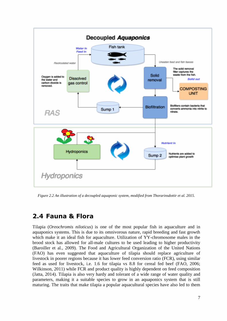
Various species of plants have been tested with success in aquaponic systems (Table 2.1).

Many studies show that leafy green plants such as various cultivars of lettuce (Latuca

sativa), basil (Ocimum basilicum) give very good yields in aquaponic systems (Rakocy et

al., 2003; Savidov et al., 2007; Trang et.al., 2010).

Table 2.1 Different kinds of plants grown in aquaponics.

Species Scientific name Reference Yield

(kg/m2/year

)

Basil Ocimum basilicum (Rakocy et al., 2003;

Savidov et al., 2007)

13-42

Lettuce Latuca sativa (Savidov et al., 2007;

Trang et al., 2010)

30

Pak-choi Brassica campestris. var. chinensis (Hu et al., 2015; Trang

et al., 2010)

3.8

(plant:feed

ratio)

Choy sum Brassica campestris. var. parachinensis (Trang et

al., 2010)

Tomato Solanum lycopersicon (Graber & Junge, 2009) 128

Water spinach Ipomoea aquatica (Liang & Chien, 2013;

Savidov et al., 2007)

60

Chives Allium schoenoprasum (Savidov et al., 2007) 14

Spinach Spinacia oleracea (Savidov et al., 2007) 15

Egg plant Solanum melongena (Graber & Junge, 2009;

Savidov et al., 2007)

32.9

Parsley Petroselinum crispum (Savidov et al., 2007) 20

Cucumber Cucumis sativus (Graber & Junge, 2009;

Savidov et al., 2007)

29.2

Watercress Nasturtium officinale (Savidov et al., 2007) 10

Okra Abelmoschus esculentus (Rakocy et al, 2004) 13,4

Staggered vegetable production seems to be favored over batch production. In Staggered

production the plants of the system are of different growth stages at all times, from

seedlings to harvest size plants allowing labor to be managed. Growing all of the plants in

the same growing phase can lead also to nutrition deficiencies while plants of different

growth stages have different nutritional requirements therefore moderating the nutrient

uptake (Rakocy et al., 2003).

9

The balance between the nitrogen waste produced in the system and plant uptake is of a

large importance, as described in section 1.2 Nitrogen metabolites carry a toxicity risk for

the animal life in the system. Plants utilize nitrogen mostly as ammonium (NH4+) or as

nitrate. Some co-influences on nutrient uptake are known such as uptake of ammonium

hinders the uptake of other cations from the substrate whereas nitrate uptake can impair the

uptake of phosphorus.(Haynes & Goh, 1978; Riley & Barber, 1971). Balance in the

concentrations of macronutrients N, P and K is therefore of utmost importance to keep the

nutrient use efficiency balanced (Janssen, 1998).

Nitrate removal through utilization is the most important function to the aquaponic system.

Plants assimilate CO2 and nitrate for the production of carbohydrates and amino acids that

will construct the body of the plant (Foyer et al., 2001). For efficient energy use during

photosynthesis a large amount of light harvesting chlorophyll proteins is necessary. The

protein that plays the major role in this is Rubisco. Rubisco is a catalyst and has a low

catalytic rate per mass of protein, therefore, for fast photosynthesis, Rubisco is needed in

large amounts. If nitrogen supply is low during the growth of the leaf, less amount of

Rubisco is formed leading to lower photosynthetic productivity in the leaf (Lawlor et al.,

1989). Rubisco also has a low affinity for CO2 therefore by increasing the concentration of

CO2 in the atmosphere, faster photosynthesis can be reached (Drake et al., 1997). However

high CO2 content in the culture water are detrimental to fish health, therefore measures

have to be taken to minimize the CO2 content.

11

3 Materials and methods

3.1 Systems

The work was carried out during a two years period from spring 2014 until spring 2016.

Aquaponics systems were developed in four different places during the development; a

show case system for visitors at Iceland Ocean Cluster House in Reykjavik; developing

units in a greenhouse in Kopavogur; and in an industry building in Reykjavik; and a small

scale commercial unit at the greenhouse farm Akur in Laugaras, South Iceland (Table 3.1).

The show case system in the Ocean Cluster House has been operational from January

2014. It has served well as an educational and presentation unit for a large group of visitors

from many different countries. In the greenhouse in Kopavogur, three systems were built

in June 2014 and operated until October the same year when they were moved to the

industry building in Reykjavik for further development. During spring 2015 the small scale

commercial unit was started in the greenhouse in Laugarás, South Iceland.

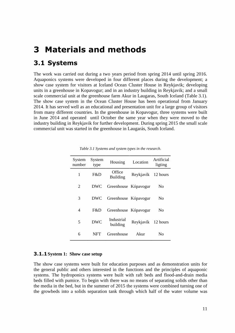
Table 3.1 Systems and system types in the research.

System

number

System

type Housing Location

Artificial

ligting

1 F&D Office

Building Reykjavík 12 hours

2 DWC Greenhouse Kópavogur No

3 DWC Greenhouse Kópavogur No

4 F&D Greenhouse Kópavogur No

5 DWC Industrial

building Reykjavík 12 hours

6 NFT Greenhouse Akur No

3.1.1 System 1: Show case setup

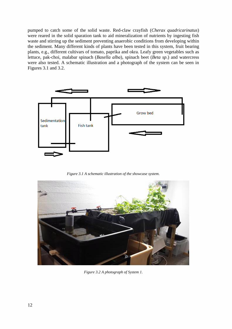
The show case systems were built for education purposes and as demonstration units for

the general public and others interested in the functions and the principles of aquaponic

systems. The hydroponics systems were built with raft beds and flood-and-drain media

beds filled with pumice. To begin with there was no means of separating solids other than

the media in the bed, but in the summer of 2015 the systems were combined turning one of

the growbeds into a solids separation tank through which half of the water volume was

12

pumped to catch some of the solid waste. Red-claw crayfish (Cherax quadricarinatus)

were reared in the solid sparation tank to aid mineralization of nutrients by ingesting fish

waste and stirring up the sediment preventing anaerobic conditions from developing within

the sediment. Many different kinds of plants have been tested in this system, fruit bearing

plants, e.g., different cultivars of tomato, paprika and okra. Leafy green vegetables such as

lettuce, pak-choi, malabar spinach (Basella alba), spinach beet (Beta sp.) and watercress

were also tested. A schematic illustration and a photograph of the system can be seen in

Figures 3.1 and 3.2.

Figure 3.1 A schematic illustration of the showcase system.

Figure 3.2 A photograph of System 1.

13

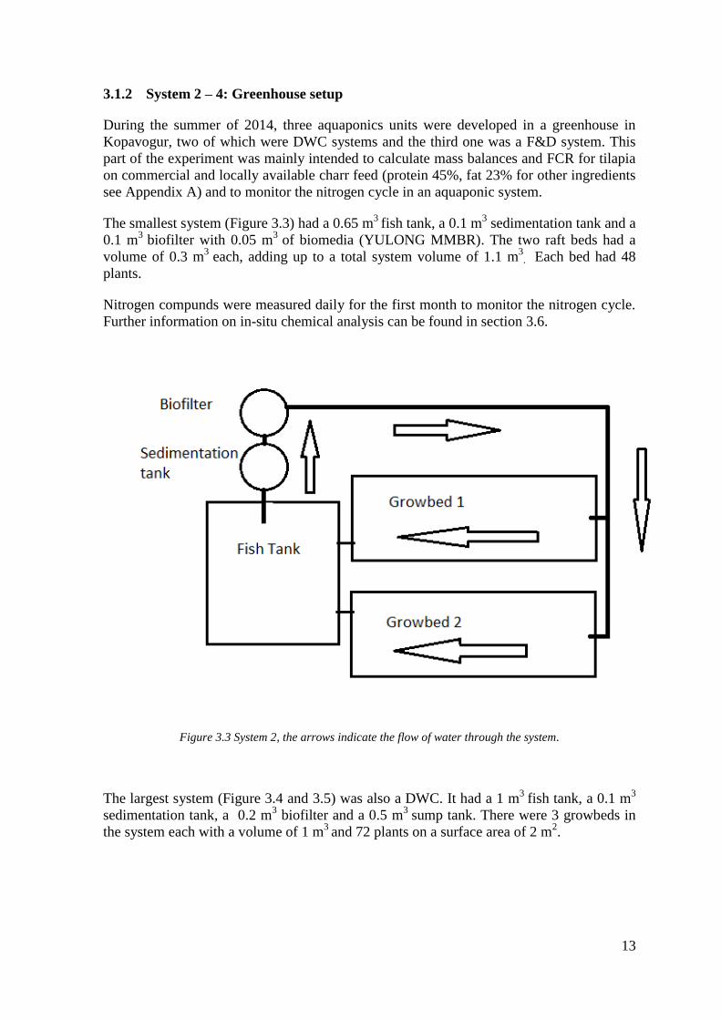
3.1.2 System 2 – 4: Greenhouse setup

During the summer of 2014, three aquaponics units were developed in a greenhouse in

Kopavogur, two of which were DWC systems and the third one was a F&D system. This

part of the experiment was mainly intended to calculate mass balances and FCR for tilapia

on commercial and locally available charr feed (protein 45%, fat 23% for other ingredients

see Appendix A) and to monitor the nitrogen cycle in an aquaponic system.

The smallest system (Figure 3.3) had a 0.65 m3

fish tank, a 0.1 m3 sedimentation tank and a

0.1 m3

biofilter with 0.05 m3

of biomedia (YULONG MMBR). The two raft beds had a

volume of 0.3 m3

each, adding up to a total system volume of 1.1 m3

. Each bed had 48

plants.

Nitrogen compunds were measured daily for the first month to monitor the nitrogen cycle.

Further information on in-situ chemical analysis can be found in section 3.6.

Figure 3.3 System 2, the arrows indicate the flow of water through the system.

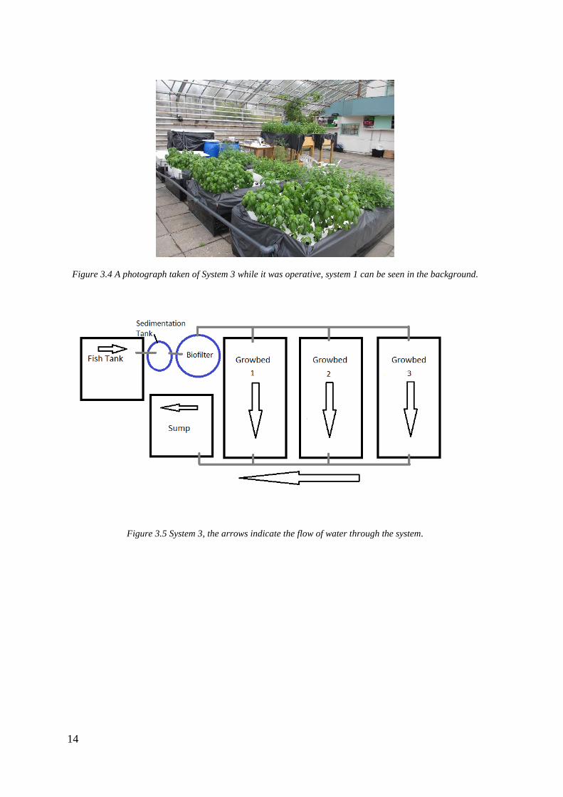
The largest system (Figure 3.4 and 3.5) was also a DWC. It had a 1 m3

fish tank, a 0.1 m3

sedimentation tank, a 0.2 m3 biofilter and a 0.5 m

3 sump tank. There were 3 growbeds in

the system each with a volume of 1 m3

and 72 plants on a surface area of 2 m2.

14

Figure 3.4 A photograph taken of System 3 while it was operative, system 1 can be seen in the background.

Figure 3.5 System 3, the arrows indicate the flow of water through the system.

15

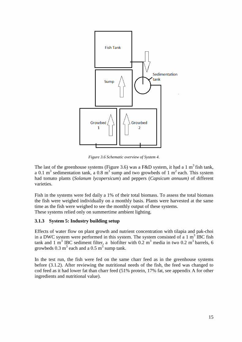
Figure 3.6 Schematic overview of System 4.

The last of the greenhouse systems (Figure 3.6) was a F&D system, it had a 1 m3

fish tank,

a 0.1 m3 sedimentation tank, a 0.8 m

3 sump and two growbeds of 1 m

2 each. This system

had tomato plants (Solanum lycopersicum) and peppers (Capsicum annuum) of different

varieties.

Fish in the systems were fed daily a 1% of their total biomass. To assess the total biomass

the fish were weighed individually on a monthly basis. Plants were harvested at the same

time as the fish were weighed to see the monthly output of these systems.

These systems relied only on summertime ambient lighting.

3.1.3 System 5: Industry building setup

Effects of water flow on plant growth and nutrient concentration with tilapia and pak-choi

in a DWC system were performed in this system. The system consisted of a 1 m3 IBC fish

tank and 1 m3 IBC sediment filter, a biofilter with 0.2 m

3 media in two 0.2 m

3 barrels, 6

growbeds 0.3 m3 each and a 0.5 m

3 sump tank.

In the test run, the fish were fed on the same charr feed as in the greenhouse systems

before (3.1.2). After reviewing the nutritional needs of the fish, the feed was changed to

cod feed as it had lower fat than charr feed (51% protein, 17% fat, see appendix A for other

ingredients and nutritional value).

16

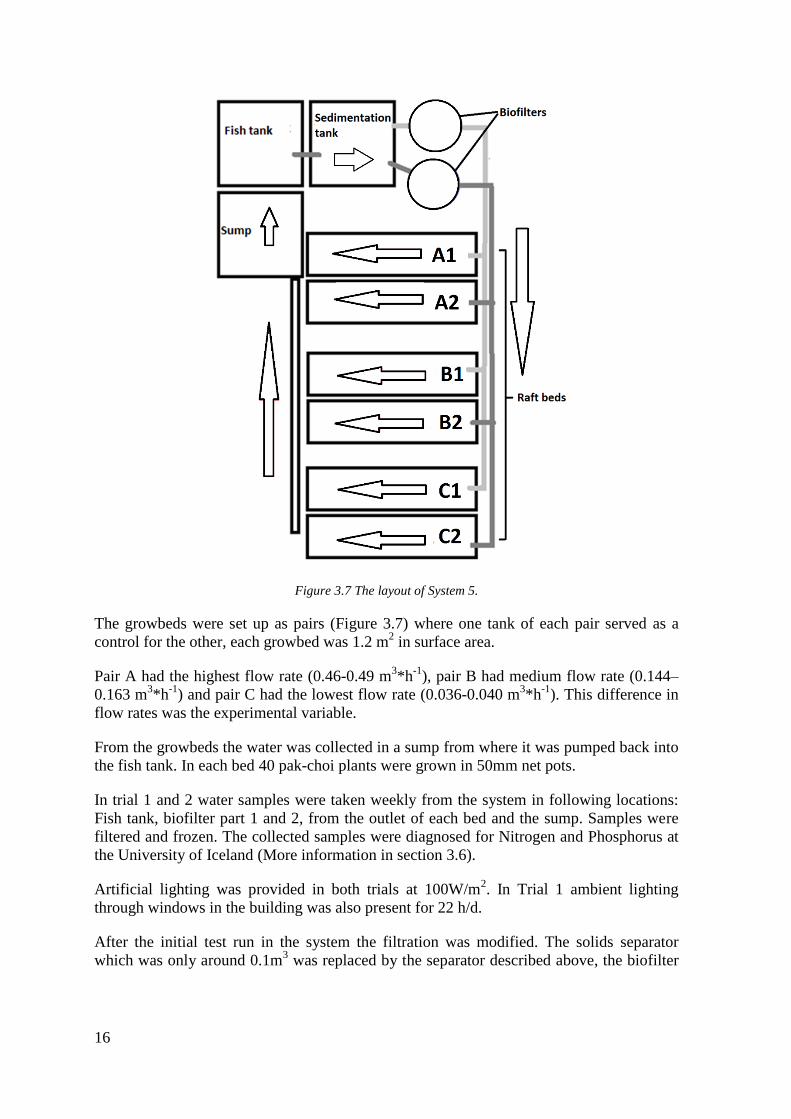
Figure 3.7 The layout of System 5.

The growbeds were set up as pairs (Figure 3.7) where one tank of each pair served as a

control for the other, each growbed was 1.2 m2 in surface area.

Pair A had the highest flow rate (0.46-0.49 m3*h

-1), pair B had medium flow rate (0.144–

0.163 m3*h

-1) and pair C had the lowest flow rate (0.036-0.040 m

3*h

-1). This difference in

flow rates was the experimental variable.

From the growbeds the water was collected in a sump from where it was pumped back into

the fish tank. In each bed 40 pak-choi plants were grown in 50mm net pots.

In trial 1 and 2 water samples were taken weekly from the system in following locations:

Fish tank, biofilter part 1 and 2, from the outlet of each bed and the sump. Samples were

filtered and frozen. The collected samples were diagnosed for Nitrogen and Phosphorus at

the University of Iceland (More information in section 3.6).

Artificial lighting was provided in both trials at 100W/m2. In Trial 1 ambient lighting

through windows in the building was also present for 22 h/d.

After the initial test run in the system the filtration was modified. The solids separator

which was only around 0.1m3 was replaced by the separator described above, the biofilter

17

which was also only 0.1m3 and contained 0.05 m

3 of media was also replaced by the filter

described.

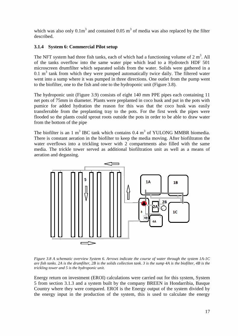
3.1.4 System 6: Commercial Pilot setup

The NFT system had three fish tanks, each of which had a functioning volume of 2 m3. All

of the tanks overflow into the same water pipe which lead to a Hydrotech HDF 501

microscreen drumfilter which separated solids from the water. Solids were gathered in a

0.1 m3 tank from which they were pumped automatically twice daily. The filtered water

went into a sump where it was pumped in three directions. One outlet from the pump went

to the biofilter, one to the fish and one to the hydroponic unit (Figure 3.8).

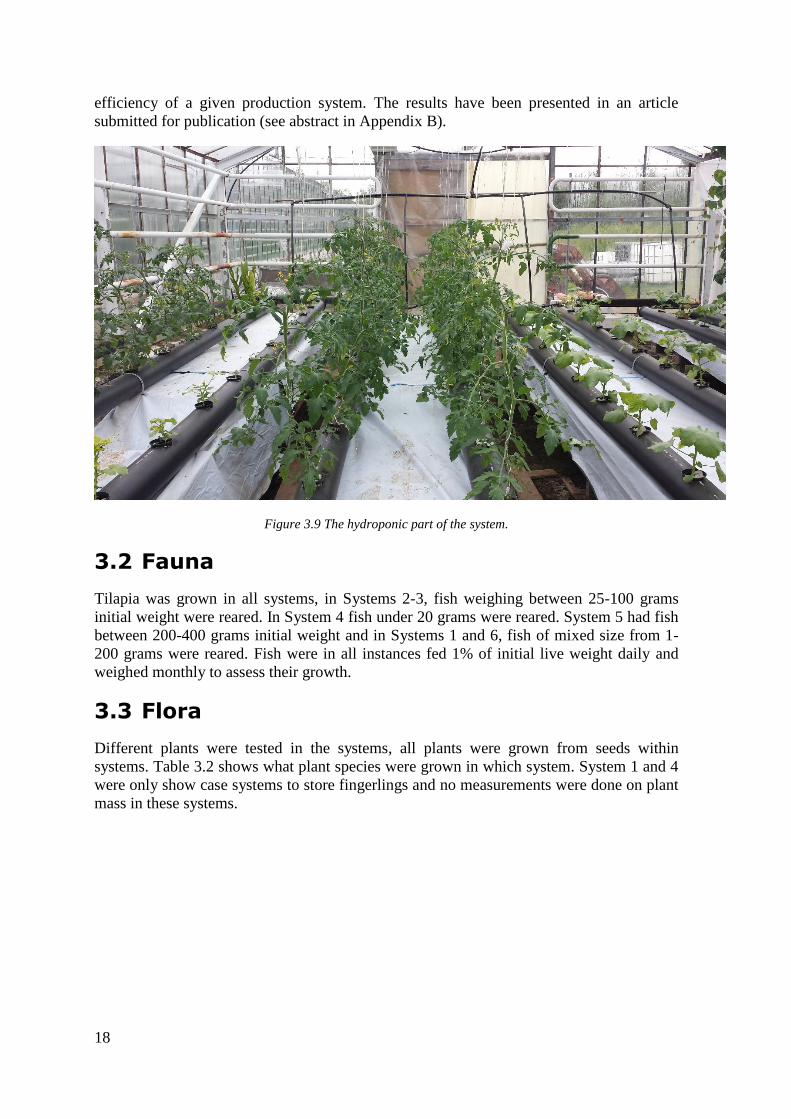
The hydroponic unit (Figure 3.9) consists of eight 140 mm PPE pipes each containing 11

net pots of 75mm in diameter. Plants were preplanted in coco husk and put in the pots with

pumice for added hydration the reason for this was that the coco husk was easily

transferrable from the preplanting tray to the pots. For the first week the pipes were

flooded so the plants could sprout roots outside the pots in order to be able to draw water

from the bottom of the pipe

The biofilter is an 1 m3 IBC tank which contains 0.4 m

3 of YULONG MMBR biomedia.

There is constant aeration in the biofilter to keep the media moving. After biofiltraton the

water overflows into a trickling tower with 2 compartments also filled with the same

media. The trickle tower served as additional biofiltration unit as well as a means of

aeration and degassing.

Figure 3.8 A schematic overview System 6. Arrows indicate the course of water through the system 1A-1C

are fish tanks. 2A is the drumfilter, 2B is the solids collection tank. 3 is the sump 4A is the biofilter, 4B is the

trickling tower and 5 is the hydroponic unit.

Energy return on investment (EROI) calculations were carried out for this system, System

5 from section 3.1.3 and a system built by the company BREEN in Hondarribia, Basque

Country where they were compared. EROI is the Energy output of the system divided by

the energy input in the production of the system, this is used to calculate the energy

18

efficiency of a given production system. The results have been presented in an article

submitted for publication (see abstract in Appendix B).

Figure 3.9 The hydroponic part of the system.

3.2 Fauna

Tilapia was grown in all systems, in Systems 2-3, fish weighing between 25-100 grams

initial weight were reared. In System 4 fish under 20 grams were reared. System 5 had fish

between 200-400 grams initial weight and in Systems 1 and 6, fish of mixed size from 1-

200 grams were reared. Fish were in all instances fed 1% of initial live weight daily and

weighed monthly to assess their growth.

3.3 Flora

Different plants were tested in the systems, all plants were grown from seeds within

systems. Table 3.2 shows what plant species were grown in which system. System 1 and 4

were only show case systems to store fingerlings and no measurements were done on plant

mass in these systems.

19

Table 3.2 plants grown in the research.

System

number

System

type Plants grown

1 F&D

Tomato, peppers, basil,

watercress, okra, pak-

choi, komatsuna

2 DWC Basil, coriander, rucola,

mint

3 DWC Basil, coriander, rucola,

mint

4 F&D Tomato and peppers*

5 DWC Pak-Choi

6 NFT Tomato and Okra

*not measured

3.4 Lighting and electrical appliances

Two systems used artificial Lighting (Table 3.1). In these systems a 400W Metal Halide

(Powerplant MH SuperVeg) bulb with a Eurowing reflector was suspended over each pair

of bed. These bulbs are stated by the manufacturere to have more light in the blue spectrum

to support vegetative growth. All Systems had impeller pumps, aerators and electronic

heaters, all manufactured by Hailea, further information on the pumps and product names

can be seen in Table 3.3.

Table 3.3 Electrical appliances used in the systems.

System Pump Q (liter/h) Heater Aerator

1 HX8830 3100 1x300W 9610

2 HX8830 3100 2x 300W 9610

3 HX8860 6500 2x300W 9810

4 HX8830 3100 No 9610

5 HX8830 3100 3x300W ACO-009

6 H18000 18000 No ACO-009

3.5 Statistical analysis

For System 5 Nested analysis of variance (ANOVA) was used to estimate the effects of

HLR, age of the system and trial on nutrient removal and a simple ANOVA was used to

compare plant yields between pairs within trials.

20

3.6 Water sampling and Chemical analysis

Weekly water samples were collected from System 5. Two 100 ml samples were gathered

from locations in the system indicated in Table 3.4. One of he samples was acidified for

storage, the other was filtered through a 40µm filter to remove any suspended solids. All

samples were frozen and then thawed for chemical analysis NO2 and NO3 were measured

using the method described in Shand et al. (2008) and Phosphorus was determined using

the method described in Murphy and Riley (1962). Mg, Ca and K are currently being

measured.

Table 3.4 Locations of sampling and number of samples taken from System 5.

Location Samples Filtered Acidified

Sump 2x 100 ml 100 ml 100 ml

fish tank 2x 100 ml 100 ml 100 ml

Biofilter 1 2x 100 ml 100 ml 100 ml

biofilter 2 2x 100 ml 100 ml 100 ml

Bed A1 2x 100 ml 100 ml 100 ml

Bed A2 2x 100 ml 100 ml 100 ml

Bed B1 2x 100 ml 100 ml 100 ml

Bed B2 2x 100 ml 100 ml 100 ml

Bed C1 2x 100 ml 100 ml 100 ml

Bed C2 2x 100 ml 100 ml 100 ml

In-situ chemical analysis were performed using Multitest NO2/NO3, Multitest Ammonia

and Multitest Phosphate also produced by Seachem Laboratories following the instruction

manuals (Appendix C). Conductivity, TDS and pH were measured using PCSTestr 35

multi-Parameter device from Eutech Instruments. Dissolved oxygen was monitored with

CyberScan DO300 manufactured by Eutech Instruments. and maintained over 4mg/l. Iron

was measured with HI checker colorimeter iron from Hanna Instruments. Iron was

maintained at 0.3 mg/l in all systems by adding AquaIron DTPA Iron Chelate.

21

4 Results

4.1 System 1

A survey was done on public opinion on aquaponics (Table 4.1). 43 people of the age

between 19 and 65 years answered the survey, 32 of which were female and 11 male. 16 of

the people had a Bachelors degree whereas 8 had a diploma or lower education and 12 had

a higher education level. 5 people did not answer. As seen in Table 4.1 most of the

participants showed a positive attitude towards aquaponic production methods and

products.

Table 4.1 Results from the survey of public opinion on aquaponics.

I Strongly

disagree (%)

I mildly

disagree(%) Neutral(%)

I mildly

agree(%)

I strongly

agree(%)

I would prefer aquaponic fish 2 7 30 26 35

I would prefer aquaponic

vegetables 2 7 35 33 23

I would not eat aquaponic

products 79 7 12 0 2

I want to know where my food

comes from 2 5 9 35 47

Aquaponics is ecological 0 0 9 37 53

Aquaponics is sustainable 2 0 7 35 53

Aquaponics supports better use

of resources 2 0 5 30 63

4.2 Systems 2-4

As can be seen in Figure 4.1 the nitrifying bacteria took a month to establish in System 2.

This can be seen in the initial TAN spike around week one followed by a decline in TAN

concentration and increase in NO2 which was subsequently exhausted in the system after

four weeks, indicating that sufficient amount of nitrifying bacteria had colonized the

system to instantly remove TAN and NO2 as they formed in the system, leaving only NO3.

22

Figure 4.1 Nitrogen data from System 2.

System 3 showed the same trend as System 2, with the exception that a spike in TAN

concentration never occurred in the system (Figure 4.2). The NO2 peaked at 5mg/l and was

maintained at that level with water exchange seen by a drop in NO3 concentration at 18.07

and another 2 days later.

Figure 4.2 Nitrogen data for System 3.

Conductivty was measured as an indicator of accumulation of nutrients within the system

as the conductivity increases with the addition of ions to the water. Nitrification is an

acidifying process and therefore pH should decrease as time progresses. This can be seen

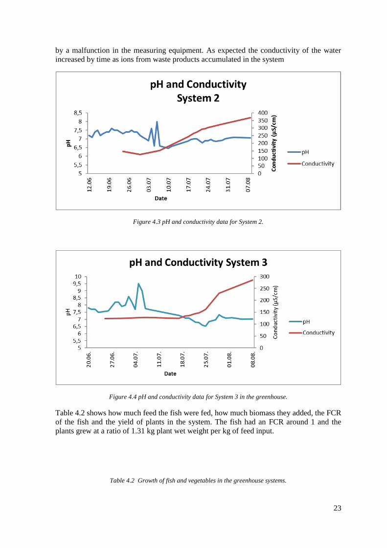
in Figures 4.3 and 4.4 where pH decreased by time except for two spikes probably caused

23

by a malfunction in the measuring equipment. As expected the conductivity of the water

increased by time as ions from waste products accumulated in the system

Figure 4.3 pH and conductivity data for System 2.

Figure 4.4 pH and conductivity data for System 3 in the greenhouse.

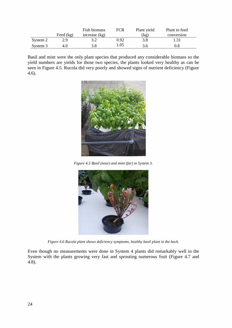
Table 4.2 shows how much feed the fish were fed, how much biomass they added, the FCR

of the fish and the yield of plants in the system. The fish had an FCR around 1 and the

plants grew at a ratio of 1.31 kg plant wet weight per kg of feed input.

Table 4.2 Growth of fish and vegetables in the greenhouse systems.

24

Feed (kg)

Fish biomass

increase (kg)

FCR Plant yield

(kg)

Plant to feed

conversion

System 2 2.9 3.2 0.92 3.8 1.31

System 3 4.0 3.8 1.05 3.6 0.8

Basil and mint were the only plant species that produced any considerable biomass so the

yield numbers are yields for those two species, the plants looked very healthy as can be

seen in Figure 4.5. Rucola did very poorly and showed signs of nutrient deficiency (Figure

4.6).

Figure 4.5 Basil (near) and mint (far) in System 3.

Figure 4.6 Rucola plant shows deficiency symptoms, healthy basil plant in the back.

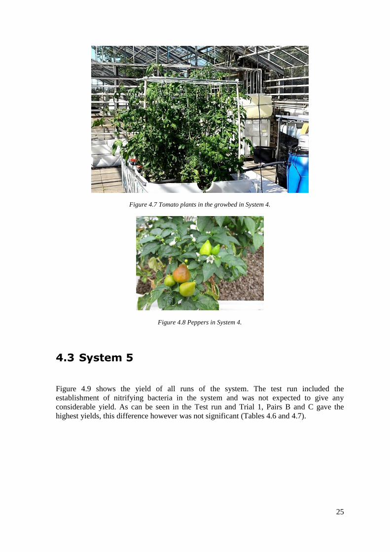
Even though no measurements were done in System 4 plants did remarkably well in the

System with the plants growing very fast and sprouting numerous fruit (Figure 4.7 and

4.8).

25

Figure 4.7 Tomato plants in the growbed in System 4.

Figure 4.8 Peppers in System 4.

4.3 System 5

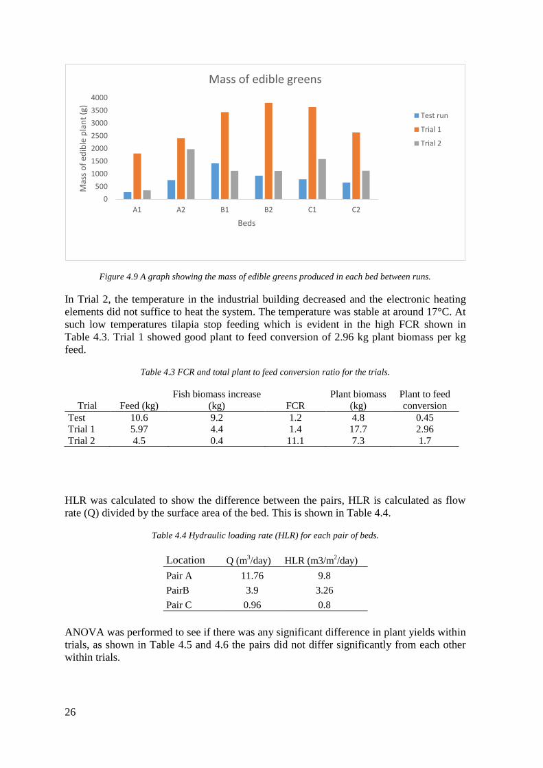
Figure 4.9 shows the yield of all runs of the system. The test run included the

establishment of nitrifying bacteria in the system and was not expected to give any

considerable yield. As can be seen in the Test run and Trial 1, Pairs B and C gave the

highest yields, this difference however was not significant (Tables 4.6 and 4.7).

26

Figure 4.9 A graph showing the mass of edible greens produced in each bed between runs.

In Trial 2, the temperature in the industrial building decreased and the electronic heating

elements did not suffice to heat the system. The temperature was stable at around 17°C. At

such low temperatures tilapia stop feeding which is evident in the high FCR shown in

Table 4.3. Trial 1 showed good plant to feed conversion of 2.96 kg plant biomass per kg

feed.

Table 4.3 FCR and total plant to feed conversion ratio for the trials.

Trial Feed (kg)

Fish biomass increase

(kg) FCR

Plant biomass

(kg)

Plant to feed

conversion

Test 10.6 9.2 1.2 4.8 0.45

Trial 1 5.97 4.4 1.4 17.7 2.96

Trial 2 4.5 0.4 11.1 7.3 1.7

HLR was calculated to show the difference between the pairs, HLR is calculated as flow

rate (Q) divided by the surface area of the bed. This is shown in Table 4.4.

Table 4.4 Hydraulic loading rate (HLR) for each pair of beds.

Location Q (m3/day) HLR (m3/m

2/day)

Pair A 11.76 9.8

PairB 3.9 3.26

Pair C 0.96 0.8

ANOVA was performed to see if there was any significant difference in plant yields within

trials, as shown in Table 4.5 and 4.6 the pairs did not differ significantly from each other

within trials.

0

500

1000

1500

2000

2500

3000

3500

4000

A1 A2 B1 B2 C1 C2

Mas

s o

f ed

ible

pla

nt

(g)

Beds

Mass of edible greens

Test run

Trial 1

Trial 2

27

Table 4.5 Results of ANOVA for plant yield between pairs in Trial 1.

Sum Sq Df Mean Sq F Pr(>F) Significance

Between 2382734 2 1191367 4.77 0.12 NS

Within 748747 3 249582

Table 4.6 Results of ANOVA for plant yield between pairs in Trial 2.

Sum Sq Df Mean Sq F Pr(>F) Significance

Between 62440.33 2 31220.167 0.066 0.94 NS

Within 1413623 3 471207.67

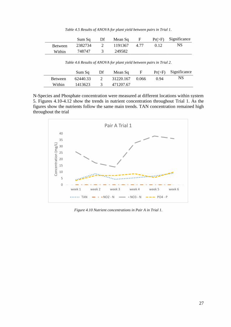
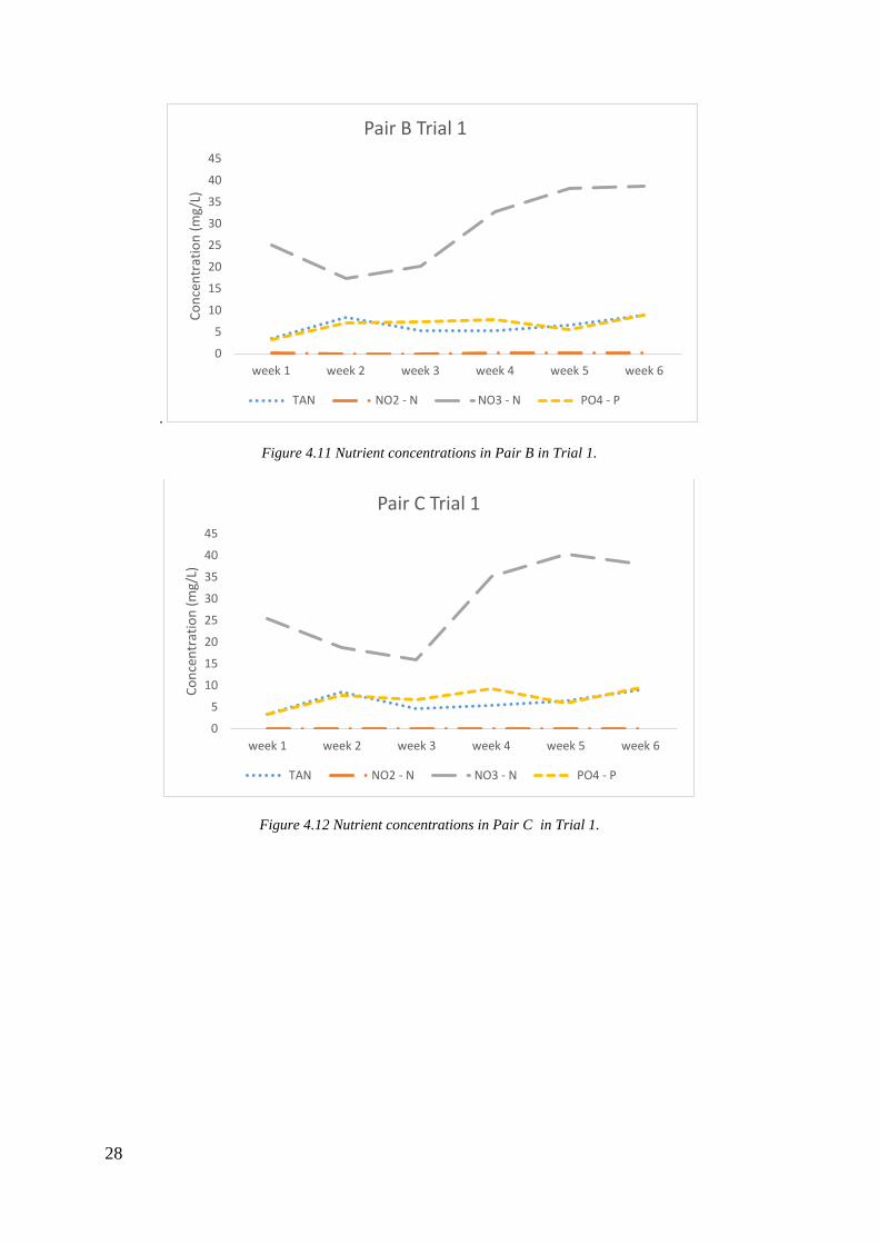
N-Species and Phosphate concentration were measured at different locations within system

5. Figures 4.10-4.12 show the trends in nutrient concentration throughout Trial 1. As the

figures show the nutrients follow the same main trends. TAN concentration remained high

throughout the trial

Figure 4.10 Nutrient concentrations in Pair A in Trial 1.

0

5

10

15

20

25

30

35

40

week 1 week 2 week 3 week 4 week 5 week 6

Co

nce

ntr

atio

n (

mg/

L)

Pair A Trial 1

TAN NO2 - N NO3 - N PO4 - P

28

.

Figure 4.11 Nutrient concentrations in Pair B in Trial 1.

Figure 4.12 Nutrient concentrations in Pair C in Trial 1.

0

5

10

15

20

25

30

35

40

45

week 1 week 2 week 3 week 4 week 5 week 6

Co

nce

ntr

atio

n (

mg/

L)

Pair B Trial 1

TAN NO2 - N NO3 - N PO4 - P

0

5

10

15

20

25

30

35

40

45

week 1 week 2 week 3 week 4 week 5 week 6

Co

nce

ntr

atio

n (

mg/

L)

Pair C Trial 1

TAN NO2 - N NO3 - N PO4 - P

29

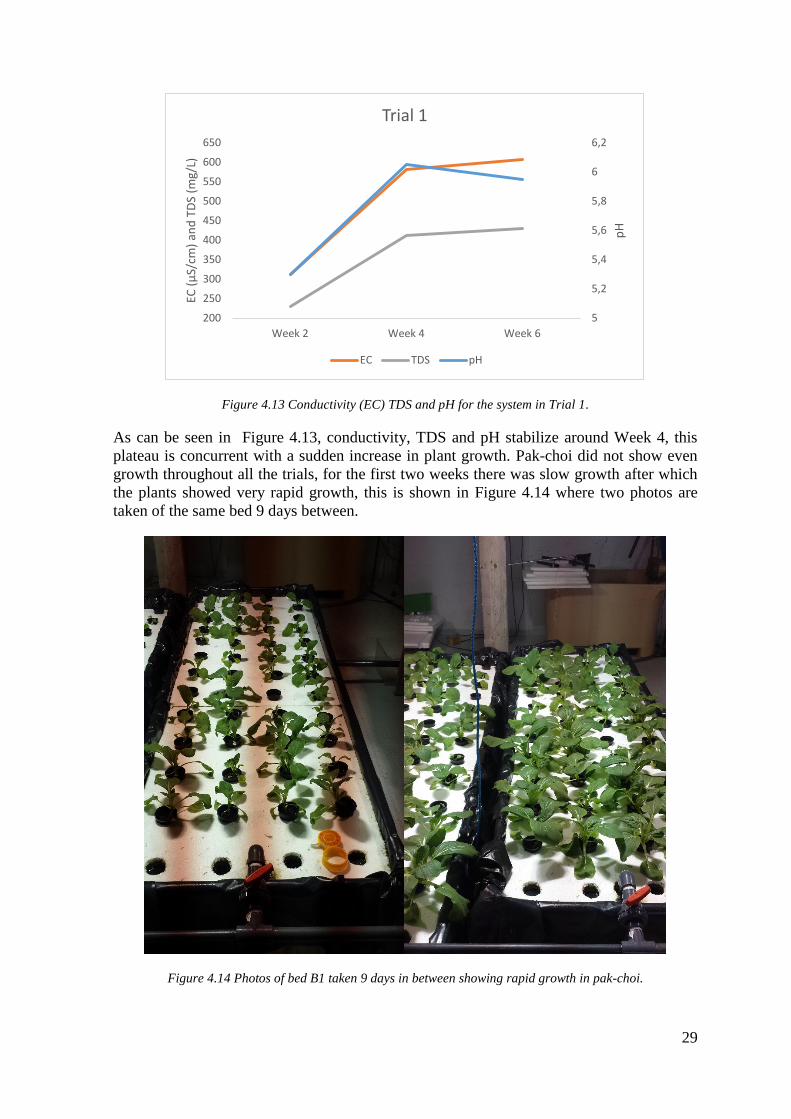
Figure 4.13 Conductivity (EC) TDS and pH for the system in Trial 1.

As can be seen in Figure 4.13, conductivity, TDS and pH stabilize around Week 4, this

plateau is concurrent with a sudden increase in plant growth. Pak-choi did not show even

growth throughout all the trials, for the first two weeks there was slow growth after which

the plants showed very rapid growth, this is shown in Figure 4.14 where two photos are

taken of the same bed 9 days between.

Figure 4.14 Photos of bed B1 taken 9 days in between showing rapid growth in pak-choi.

5

5,2

5,4

5,6

5,8

6

6,2

200

250

300

350

400

450

500

550

600

650

Week 2 Week 4 Week 6

pH

EC (

µS/

cm)

and

TD

S (m

g/L)

Trial 1

EC TDS pH

30

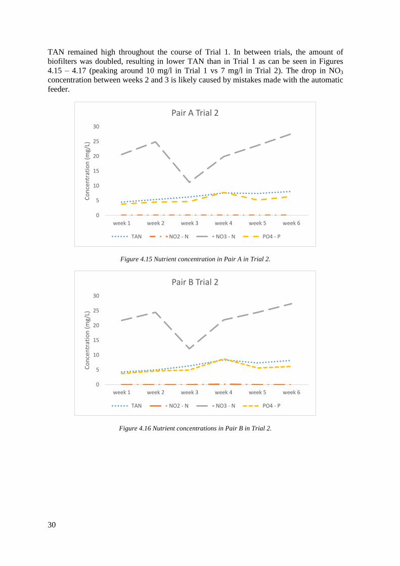
TAN remained high throughout the course of Trial 1. In between trials, the amount of

biofilters was doubled, resulting in lower TAN than in Trial 1 as can be seen in Figures

4.15 – 4.17 (peaking around 10 mg/l in Trial 1 vs 7 mg/l in Trial 2). The drop in NO3

concentration between weeks 2 and 3 is likely caused by mistakes made with the automatic

feeder.

Figure 4.15 Nutrient concentration in Pair A in Trial 2.

Figure 4.16 Nutrient concentrations in Pair B in Trial 2.

0

5

10

15

20

25

30

week 1 week 2 week 3 week 4 week 5 week 6

Co

nce

ntr

atio

n (

mg/

L)

Pair A Trial 2

TAN NO2 - N NO3 - N PO4 - P

0

5

10

15

20

25

30

week 1 week 2 week 3 week 4 week 5 week 6

Co

nce

ntr

atio

n (

mg/

L)

Pair B Trial 2

TAN NO2 - N NO3 - N PO4 - P

31

Figure 4.17 Nutrient concentrations in Pair C in Trial 2.

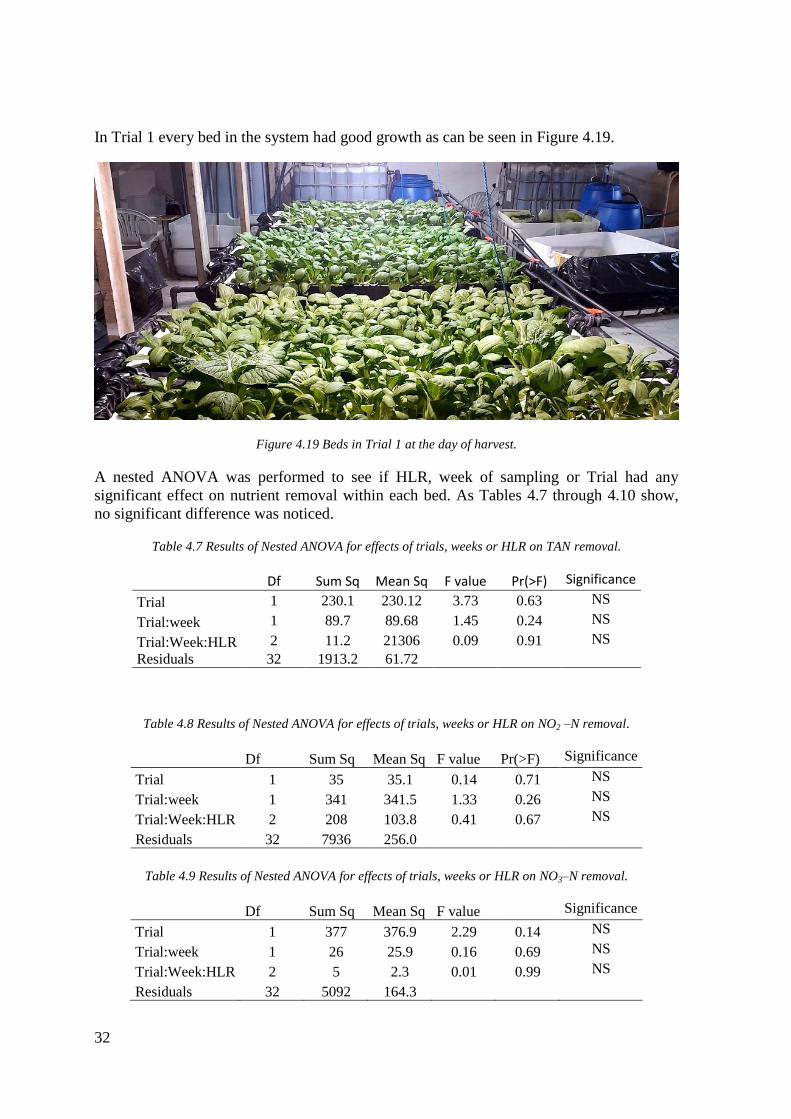
When looking at pH, conductivity and TDS for the system (Figure 4.18) pH drops between

weeks 1 and 3 and rises again from week 3 to 5. This is concurrent with the drop in NO3

between weeks 2 and 3 (Figures 4.15 to 4.17). The little increase in conductivity and TDS

between weeks 2 and 3 is explained by a mistake made with the automatic feeder.

Figure 4.18 Conductivity (EC) TDS and pH for the system in Trial 2.

0

5

10

15

20

25

30

week 1 week 2 week 3 week 4 week 5 week 6

Co

nce

ntr

atio

n (

mg/

L)

Pair C Trial 2

TAN NO2 - N NO3 - N PO4 - P

4,8

4,9

5

5,1

5,2

5,3

5,4

5,5

5,6

5,7

5,8

300

350

400

450

500

550

Week 1 Week 2 Week 3 Week 5

pH

EC (

µS/

cm)

and

TD

S (m

g/L)

Trial 2

EC TDS pH

32

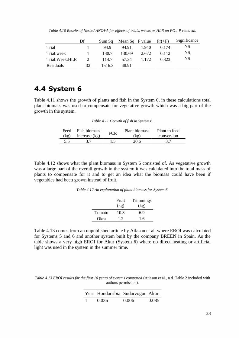
In Trial 1 every bed in the system had good growth as can be seen in Figure 4.19.

Figure 4.19 Beds in Trial 1 at the day of harvest.

A nested ANOVA was performed to see if HLR, week of sampling or Trial had any

significant effect on nutrient removal within each bed. As Tables 4.7 through 4.10 show,

no significant difference was noticed.

Table 4.7 Results of Nested ANOVA for effects of trials, weeks or HLR on TAN removal.

Df Sum Sq Mean Sq F value Pr(>F) Significance

Trial 1 230.1 230.12 3.73 0.63 NS

Trial:week 1 89.7 89.68 1.45 0.24 NS

Trial:Week:HLR 2 11.2 21306 0.09 0.91 NS

Residuals 32 1913.2 61.72

Table 4.8 Results of Nested ANOVA for effects of trials, weeks or HLR on NO2 –N removal.

Df Sum Sq Mean Sq F value Pr(>F) Significance

Trial 1 35 35.1 0.14 0.71 NS

Trial:week 1 341 341.5 1.33 0.26 NS

Trial:Week:HLR 2 208 103.8 0.41 0.67 NS

Residuals 32 7936 256.0

Table 4.9 Results of Nested ANOVA for effects of trials, weeks or HLR on NO3–N removal.

Df Sum Sq Mean Sq F value Significance

Trial 1 377 376.9 2.29 0.14 NS

Trial:week 1 26 25.9 0.16 0.69 NS

Trial:Week:HLR 2 5 2.3 0.01 0.99 NS

Residuals 32 5092 164.3

33

Table 4.10 Results of Nested ANOVA for effects of trials, weeks or HLR on PO4–P removal.

Df Sum Sq Mean Sq F value Pr(>F) Significance

Trial 1 94.9 94.91 1.940 0.174 NS

Trial:week 1 130.7 130.69 2.672 0.112 NS

Trial:Week:HLR 2 114.7 57.34 1.172 0.323 NS

Residuals 32 1516.3 48.91

4.4 System 6

Table 4.11 shows the growth of plants and fish in the System 6, in these calculations total

plant biomass was used to compensate for vegetative growth which was a big part of the

growth in the system.

Table 4.11 Growth of fish in System 6.

Feed

(kg)

Fish biomass

increase (kg) FCR

Plant biomass

(kg)

Plant to feed

conversion

5.5 3.7 1.5 20.6 3.7

Table 4.12 shows what the plant biomass in System 6 consisted of. As vegetative growth

was a large part of the overall growth in the system it was calculated into the total mass of

plants to compensate for it and to get an idea what the biomass could have been if

vegetables had been grown instead of fruit.

Table 4.12 An explanation of plant biomass for System 6.

Fruit

(kg)

Trimmings

(kg)

Tomato 10.8 6.9

Okra 1.2 1.6

Table 4.13 comes from an unpublished article by Atlason et al. where EROI was calculated

for Systems 5 and 6 and another system built by the company BREEN in Spain. As the

table shows a very high EROI for Akur (System 6) where no direct heating or artificial

light was used in the system in the summer time.

Table 4.13 EROI results for the first 10 years of systems compared (Atlason et al., n.d. Table 2 included with

authors permission).

Year Hondarribia Sudarvogur Akur

1 0.036 0.006 0.085

34

2 0.045 0.007 0.099

3 0.049 0.007 0.102

4 0.051 0.008 0.104

5 0.052 0.008 0.105

6 0.053 0.008 0.106

7 0.054 0.008 0.107

8 0.055 0.008 0.107

9 0.055 0.008 0.107

10 0.055 0.008 0.108

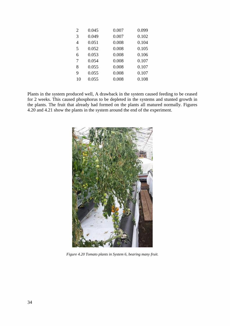
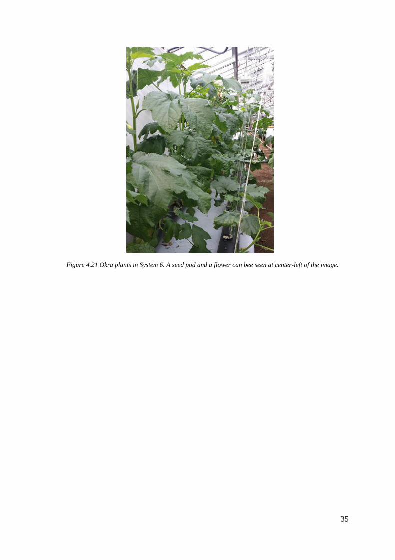
Plants in the system produced well, A drawback in the system caused feeding to be ceased

for 2 weeks. This caused phosphorus to be depleted in the systems and stunted growth in

the plants. The fruit that already had formed on the plants all matured normally. Figures

4.20 and 4.21 show the plants in the system around the end of the experiment.

Figure 4.20 Tomato plants in System 6, bearing many fruit.

35

Figure 4.21 Okra plants in System 6. A seed pod and a flower can bee seen at center-left of the image.

37

5 Discussion

System 1, The Showcase system, has been a successful demonstration of the neccessity of

proper solids removal. For the first year there were no visible effects but early in 2015 fish

started showing symptoms of deficiencies and stress. Instability in water conditions was

caused by buildup of solids in the system and following a cleaning of the substrate media

there was an ammonia spike that had to be remedied by rapid water changes for 3

consecutive days. After the addition of a settling tank a considerable amount of solids has

been removed from the system. Worms (Eisenia fetida) were added to the media bed to aid

with mineralization of the solids accumulating in the media and in the settling tank were

seven red-clawed-crayfish that constantly sifted through the accumulated solids. The

settling tank where the crayfish lived had a bottom area of around 1m2

and was littered

with PVC pipes for shelter. Some aggression and cannibalism was noted in the crayfish

indicating that they feel confined, this could be remedied by adding more pipes and hiding

places for them as stocking densities of up to 60 crayfish per m2 should be feasible for

breeding them (Barki & Karplus, 2000). Adding more pipes could also aid in catching

solids and minimizing direct current within the settling tank. Leafy green plants have

performed well in the system especially basil which produced enough to be distributed

promotionally. Fruit bearing plants did not thrive as well. Tomatoes rarely flowered with

around one flower per month. Okra showed mostly vegetative growth in the system. The

low productivity of fruit bearing plants is likely due to the stable warm conditions in the

office and unfavourable nutrient profile in the system. In April 2015 plants started showing

symptoms of stress again. Chlorosis, often associated with Fe deficiency was noted. Fe was

measured at 1mg/L in the water column A thorough cleaning of the media was done

revealing large amounts of accumulated solids in the media. Following the cleaning the

deficiency symptoms disappeared leading to suspicion of salt stress or other unfavourable

conditions forming in the growing medium. Salt stress increases suberization of root

endothelium leading to the plants stopping active absorbtion of nutriets (Barberon et al.,

2015).

In Systems 2 and 3 rucola showed purple leaves and stunted growth which are symptoms

of phosphorus deficiency (Bradley & Hosier, 1999). When measured, phosphorus was in

good supply (3 mg/L) in the water and the water pH was 6.4. Phosphorus uptake is pH

sensitive (Bradley & Hosier, 1999) so suspicion rose that the pH within the peat insert was

too low. A supporting argument for that was that the plants which showed signs of

deficiencies had no roots outside the insert and were therefore not in direct contact with the

water. A decision was made to add CaCO3 additive, Hafkorn (ingredients in Appendix A),

to the system. The symptoms of deficiency disappeared partly even though some of the

plants did still show stunted growth. Those that did best managed to sprout roots outside

the peat and into the water leading to the assumption that the pH in the peat was too low to

allow for proper nutrient uptake and healthy growth.

There was a noticeable amount of solids in all of the growbeds in the systems underlining

the necessity for better solids removal. In the end the roots on some of the plants in System

2 became clogged and rotted away. In one instance in the greenhouse systems hydrogen

sulphide smell was noticed in one of the growbeds indicating anaerobic conditions within

38

the sediment. This could have been alleviated by both increasing solids filtration and by

increasing water movement in the growbeds to keep the solids in suspension instead of

accumulating in the beds. Where the hydroponic part of the system is small solids should

be removed from the system as they are far in excess of what the plants will manage to

regulate (Rakocy, 1999).

After slaughtering fish from Systems 2 and 3 it became evident that the charr feed might

not be suitable for them. Tilapia mainly collect fat in visceral adipose tissue (He et al.,

2015) in fact the internal organs were all combined in a white mass of fat that had to be

removed to view the organs. The decision was made to switch to a lower fat feed than

charr feed (17% Cod feed vs 23% Charr feed) this would still be considered a high fat feed

for tilapia with 5 – 7.4 % fat being the optimum (He et al., 2015).

In System 5 the beds with the fastest flow showed the least biomass produced and also the

most solids buildup. Even though not measured there were visibly more solids that covered

the roots of these plants, especially in the Test run and Trial 1. The slower flow beds, pairs

B and C, produced more biomass, and had less solids built up on the roots. After officially

ending Trial 1 the plants were put back in the system with their protruding roots removed.

In a week the plants in all beds showed a minor increase in growth with healthy root

growth also, indicating that solids buildup was having negative effect on them.

There was no significant difference found in mass due to HLR in the beds (Tables 5.3 and

5.4). Light and temperature were different between the two trials and made the largest

contribution to the difference in mass between those two. Sudden drop in NO3 between

weeks 2 and three in Trial 2 is probably due to a mistake made with the automatic feeder as

the feeder looked half full when in fact it was clogged and therefore no feed was added to

the system for that week, interestingly, no drop in TAN concentration was observed.

No weekly measurements of plants were made so the contribution of weekly growth on

nutrient content could not be evaluated. Plant growth, however, was not linear, the plants

stayed small for around 2-3 weeks and suddenly showed a rapid growth. The production

cycle of the plants from seed to harvest took 6 weeks and yielded 1.01 (Trial 2) - 2.45

(Trial 1) kg/m2. This yield is within the same variable yields found for lettuce in

aquaponics (1.4 - 6.5 kg/m2) (Rakocy et al., 1997; Seawright et al., 1998). Pak-choi can be

very fast growing and demand after fresh pak-choi has grown with the diversifying

population of Iceland. The success of pak-choi also underlines the success of leafy green

vegetables grown in aquaponic systems and indicates that even more, commercially

valuable, species with similar requirements can be successfully grown in this kind of

system. There was no significant difference in plant nutrient removal between trials, beds

nor HLR, the largest contributing factor on plant mass was light, as in Trial 1 ambient

light was present through windows leading to to the suspicion that the hydroponic part of

this system could have been larger with lower HLR rates to support more production than

seen in this system. This is further supported by the fact that NO3 and PO4 concentrations

continued to rise and the nutrient utilization of the plants present in the system was

therefore not enough to regulate the nutrient concentrations (Rakocy, 1999).

The statistical tests done in System 5 are of little quality as the sample size (2 trials) was

very low. Further research with a larger sample are needed to give conclusive results.

39

The okra plants in System 6 could have produced more seed pods than they did. The

flowers would close and fall off as expected but the developing pods would die within two

days with less than 30% reaching harvest size. There was a drawback in the system where

feeding had to be stopped for two weeks and two weeks later the irrigation pipe to the

hydroponic unit was clogged for a whole day putting the plants under water stress from

evaporation. These drawbacks could have played a role in the plants sacrificing their pods

as reduced yield is a consequence of water stress (Gunawardhana & Silva, 2011). At the

same time the tomato plants were in full bloom and started showing deficiency symptoms

such as stunted growth in the plants themselves along with purple leaves. When water tests

were done phosphate was nonexistent in the system which was in accordance with the

deficiency symptoms (Bradley & Hosier, 1999). Flowering of the plants promptly halted

yet the tomatoes, which had already formed, all matured normally leading to the suspicion

that if the irrigation and feeding would have continued as normal the production would

have been much better, also bees were always present in the greenhouse so lack of

pollination is an unlikely cause. A decoupled system as described in Thorarinsdottir et al.

(2015) would have allowed for treatment of the fish system without negative effects on the

plants as they could have been supplemented in separation from the fish.

The EROI results show that building the system inside a greenhouse is more energy

efficient than building in an industry building with traditional artificial lighting. These

results though would only be relevant to summer time as the test was carried out in

summer where no artificial lighting was used in the Akur system. Artificial lighting with

LED lamps might help with more energy efficient system, LEDs have a longer lifespan

and do not produce large amounts of radiant heat as traditional HPS and MH lamps do.

Also LED is very customizable as the spectrum of light can be easily tampered with by

increasing or decreasing the ratio of red vs blue LEDs. The energy efficiency of LED

lamps is dependent on lamp design as blue LEDs use more energy than red LEDs do

(Currey & Lopez, 2013). LED lamps also allow for better spatial utilization by stacking

growbeds vertically with low profile lighting units suspended beneath the beds. Heat from

LED lamps can in that way be used for heating the water in the system.

The FCR of the fish is lowest in Systems 2 and 3 and highest in Trial 2 in System 5. This

can be contributed to two factors; the initial size of the fish and temperature. In Systems 2

and 3 the temperature was at all times higher than 21°C and the fish were at a small size of

less than 100 g per individual. In Trial 1 in System 5 temperature was stable at 21°C but

the fish were a lot larger 250g< but still growing considerably fast. Troubles with

temperature regulation in Trial 2 likely contribute the most to the slow growth of the fish in

the system as tilapia feeding and metabolism slows at temperatures below 20°C (Rakocy,

1999). The FCR of 1.0-1.5 is within the range often experienced with tilapia. The fish were

fed with feed that had a very high protein and fat content.

For better TAN removal for high protein feed at high stocking densities setting up a larger

biofilter would be necessary, perhaps a fixed bed filter or a moving bed filter with la larger

surface area. Moving bed filters do not react as well to elevated ammonia levels as fixed

bed filters. This could be contributed by the factor that biofilm is constantly being rubbed

off the outer surface of the biomedia (Suhr & Pedersen, 2010). This was evident, both in

the Industry building system in Reykjavík and in the Pilot commercial unit as no NO2 was

present in the system but TAN levels remained high. A low rate of nitrification could also

be due to the low pH, even though it has been shown that a high rate of nitrification can be

achieved at pH as low as 4.3 ( Tarre & Green, 2004).

40

Systems 5 and 6 both would have needed a larger hydroponic unit and might have

benefitted from being designed in a decoupled manner. That way nitrogen levels in the fish

tank could have been kept at more desirable levels. Due to the low pH of System 5 the high

TAN concentration was most likely in the form of NH4+

which is less harmful for fish

(Randall & Tsui, 2002). Also a long exposure to high levels of nitrate can have a negative

effect on hemoglobin in the fish (Jensen, 1996). CO2 addition increases photosynthesis in

the plant, increasing nitrogen uptake, whereas the fish rearing system design aims to

minimize CO2 levels within the system as increased CO2 impairs the growth of the fish

(Stiller et al., 2015).

The visitors to the systems have been from diverse groups, e.g. young children, high school

and university students, entrepreneurs, researchers, aquaculture and horticulture people,

policy advisors and people from government and municipalities, such as the US

ambassadeur and the president of Iceland. The results of the survey show that people have

a positive opinion on aquaponics. More people in Iceland are becoming environmentally

conscious and want to know where their food comes from and how it was produced.

The results have been presented at Aquaculture Europe 2014 in Spain, at the Science Day

at the University of Iceland in September 2015, at a seminar in Reykjavik in June 2015, at

the COST training programme held at Solheimar Iceland in September 2015 and at the

Icelandic Biology conference in October 2015, see Appendix B.

41

6 Conclusions and recommendations.

Both feed types used in this research were too high in fat and protein leading to fat deposits

around the visceral organs of the fish and very high TAN concentrations in the water and

would not be considered suitable for tilapia production. Pak-choi gave a good yield:feed

ratio of 3:1 which is suspected to be even higher in a larger hydroponic unit. No significant

effects of water flow on plant growth and nutrient uptake were measured leading to the

conclusion that the hydroponic production part of system 5 could have been larger than it

was.

The failure of fruiting plants in this research is more related to system flaws than suitability

issues as tomatoes and okra are known to show good yields in aquaponic production.

For establishing Aquaponic systems for industrial production I give these following

recommendations on system design based on the findings of this research.

1. Good particulate filtration is necessary. This could be done with a combination of

a settling tank, to remove larger particles and a microscreen drum filter, as in

System 6, to remove the finer matter. All of the systems built showed some

accumulation of solids in the hydroponic beds, the least solids were encountered in

System 6 which had the most effective filter.

2. NFT systems are more vulnerable to mishaps than DWC and F&D systems. In the

case of pump failure the NFT have very little water present at the roots of the plants

whereas DWC has the roots submerged in water and the substrate in the F&D beds

has very good moisture retention. For the longevity of the F&D system the bed has

to be cleaned regularly as solids will build up in the media, regardless of filtration

methods, and are hard to flush out without manually removing and rinsing the

media.

3. For lower TAN concentration feed with a lower protein content than used in this

experiment would be more feasible, This could also be done by improving biofilter

design e.g. by using media that has a larger surface area. Another way of dealing

with this would be removing more of the solids from the system mineralizing them

in a separate container before releasing nutrients back into the system.

4. For less compromise between optimal conditions for fish rearing and hydroponic

plant production a decoupled design would be preferred as the plants prefer higher

nutrient and CO2 concentrations, both of which have negative effect on the fish.

5. Leafy green vegetables with similar requirements as lettuce and pak-choi might be

a good choice for production in a larger scale system. Further research into plant

choices looking into current hydroponic production is necessary.

.

42

43

References

Atlason, R. S., Danner, R. I., Unnthorsson, R., Oddsson, G. V., Sustaeta, F., &

Thorarinsdottir, R. (n.d.). Improving operations based on Energy Return on

Investment : case studies from Icelandic and Spanish aquaculture. Submitted to:

Journal of Cleaner Production, 1–11.

Barberon, M., Engelbertus, J., Vermeer, M., De Bellis, D., Takano, J., Salt, D. E., Geldner,

N., Wang, P., Naseer, S., Andersen, T.G., Humbel, B.M., Nawrath, C. (2015).

Adaptation of Root Function by Nutrient-Induced Plasticity of Endodermal

Differentiation. Cell, 164, 1–13

Barki, A., & Karplus, I. (2000). Crowding female red claw crayfish, Cherax

quadricarinatus, under small-tanks hatchery conditions: What is the limit?

Aquaculture, 181(3-4), 235–240. http://doi.org/10.1016/S0044-8486(99)00235-5

Baroiller, J. F., D’Cotta, H., Bezault, E., Wessels, S., & Hoerstgen-Schwark, G. (2009).

Tilapia sex determination: Where temperature and genetics meet. Comparative

Biochemistry and Physiology - A Molecular and Integrative Physiology, 153(1), 30–

38. http://doi.org/10.1016/j.cbpa.2008.11.018

Bradley, L., & Hosier, S. (1999). Guide to Symptoms of Plant Nutrient Deficiencies. The

University of Arizona Cooperative Extension, AZ1106, 1–3.

Cheng, S.-Y., & Chen, J.-C. (2002). Study on the oxyhemocyanin, deoxyhemocyanin,

oxygen affinity and acid–base balance of Marsupenaeus japonicus following exposure

to combined elevated nitrite and nitrate. Aquatic Toxicology, 61(3-4), 181–193.

http://doi.org/10.1016/S0166-445X(02)00053-X

Currey, C. J., & Lopez, R. G. (2013). Comparing LED Lighting To High-Pressure Sodium

Lamps. Greenhouse Grower, (October).

Deane, E. E., & Woo, N. Y. S. (2007). Impact of nitrite exposure on endocrine,

osmoregulatory and cytoprotective functions in the marine teleost Sparus sarba.

Aquatic Toxicology (Amsterdam, Netherlands), 82(2), 85–93.

http://doi.org/10.1016/j.aquatox.2007.02.004

Doblander, C., & Lackner, R. (1996). Metabolism and detoxification of nitrite by trout

hepatocytes. Biochimica et Biophysica Acta - General Subjects, 1289(2), 270–274.

http://doi.org/10.1016/0304-4165(95)00166-2

Drake BG, Gonzalez-Meler MA, L. S. (1997). More efficient plants: a consequence of

rising atmospheric CO2? Annual Review of Plant Physiology and Plant Molecular

Biology, 48, 609–639. http://doi.org/10.1146/annurev.arplant.48.1.609

FAO. (2006). Livestock’s long shadow - environmental issues and options. Food and

Agriculture Organization of the United Nations, 3(1), 1–377.

http://doi.org/10.1007/s10666-008-9149-3

Fewtrell, L. (2004). Drinking Water Nitrate, Methaemoglobinaemia and Global Burden of

Disease: A Discussion. Environmental Health Perspectives, 112(14), 1371–1374.

44

http://doi.org/10.1289/ehp.7216

Foyer, C. H., Ferrario-Méry, S., & Noctor, G. (2001). Interactions Between Carbon and

Nitrogen Metabolism. In P. J. Lea & J.-F. Morot-Gaudry (Eds.), Plant Nitrogen (pp.

237–254). Berlin, Heidelberg: Springer Berlin Heidelberg. http://doi.org/10.1007/978-

3-662-04064-5_9

Graber, A., & Junge, R. (2009). Aquaponic Systems: Nutrient recycling from fish

wastewater by vegetable production. Desalination, 246(1-3), 147–156.

http://doi.org/10.1016/j.desal.2008.03.048

Gunawardhana, M. D. M., & Silva, C. S. De. (2011). Impact of Temperature and Water

Stress on Growth Yield and Related Biochemical Parameters of Okra, 23(1), 77–83.

Haynes, R. J., & Goh, K. M. (1978). AMMONIUM AND NITRATE NUTRITION OF

PLANTS. Biological Reviews, 53(4), 465–510. http://doi.org/10.1111/j.1469-

185X.1978.tb00862.x

He, A., Ning, L., Chen, L., Chen, Y., Xing, Q., Li, J., Qiao, F., Li, D., Zhang, M., Du, Z.

(2015). Systemic adaptation of lipid metabolism in response to low‐ and high‐ fat

diet in Nile tilapia ( Oreochromis niloticus ). Physiological Reports, 3(8), e12485.

http://doi.org/10.14814/phy2.12485

Hu, Z., Lee, J. W., Chandran, K., Kim, S., Brotto, A. C., & Khanal, S. K. (2015). Effect of

plant species on nitrogen recovery in aquaponics. Bioresource Technology, 188, 92–8.

http://doi.org/10.1016/j.biortech.2015.01.013

Janssen, B. H. (1998). Efficient use of nutrients: An art of balancing. Field Crops

Research, 56(1-2), 197–201. http://doi.org/10.1016/S0378-4290(97)00130-5

Jatta, S. (2014). The effects of substituting fishmeal with rapeseed meal at three protein

levels on growth and body composition of Nile tilapia fingerlings (Oreochromis

niloticus). United Nations University Fisheries Training Programme, Iceland [Final

Project].

Jensen, F. B. (1996). Uptake, elimination and effects of nitrite and nitrate in freshwater

crayfish (Astacus astacus). Aquatic Toxicology, 34(2), 95–104.

http://doi.org/10.1016/0166-445X(95)00030-8

Jensen, F. B. (2003). Nitrite disrupts multiple physiological functions in aquatic animals.

Comparative Biochemistry and Physiology - A Molecular and Integrative Physiology,

135(1),9–24.http://doi.org/10.1016/S1095-6433(02)00323-9

Kloas, W., Groß, R., Baganz, D., Graupner, J., Monsees, H., Schmidt, U., Staaks, G., Suhl,

J., Tschirner, M., Wittstock, B., Wuertz, Z., Zikova, A., Rennert, B. (2015). A new

concept for aquaponic systems to improve sustainability, increase productivity, and

reduce environmental impacts. Aquaculture Environment Interactions, 7(2), 179–192.

http://doi.org/10.3354/aei00146

Kroupova, H., Machova, J., & Svobodova, Z. (2005). Nitrite influence on fish: A review.

Veterinarni Medicina, 50(11), 461–471.

Lawlor, D. W., Kontturi, M., & Young, A. T. (1989). Photosynthesis by Flag Leaves of

Wheat in Relation to Protein, Ribulose Bisphosphate Carboxylase Activity and

Nitrogen Supply. Journal of Experimental Botany.

45

Lekang, O. I. (2007). Aquaculture Engineering. Aquaculture Engineering.

http://doi.org/10.1002/9780470995945

Liang, J.-Y., & Chien, Y.-H. (2013). Effects of feeding frequency and photoperiod on

water quality and crop production in a tilapia–water spinach raft aquaponics system.

International Biodeterioration & Biodegradation, 85, 693–700.

http://doi.org/10.1016/j.ibiod.2013.03.029

Love, D. C., Fry, J. P., Genello, L., Hill, E. S., Frederick, J. A., Li, X., & Semmens, K.

(2014). An international survey of aquaponics practitioners. PLoS ONE, 9(7).

http://doi.org/10.1371/journal.pone.0102662

Murphy, J., & Riley, J. P. (1962). A modified single solution method for the determination

of phosphate in natural waters. Analytica Chimica Acta, 27, 31–36.

http://doi.org/10.1016/S0003-2670(00)88444-5

Rakocy, J., Shultz, R. C., Bailey, D. S., & Thoman, E. S. (2003). Aquaponic production of

tilapia and basil: comparing a batch and staggered cropping system. In South Pacific

Soilless Culture Conference-SPSCC 648, 63–69.

Rakocy, J. (1999). The status of aquaponics, Part 1. Aquaculture Engineering, (August).

Rakocy, J. E. (1988). Hydroponic lettuce production in a recirculating fish culture system.

Island Perspectives, 1989(3), 4–10.

Rakocy, J. E. (1989). Tank Culture of tilapia. Southern Regional Aquaculture Center,

Publication No. 282.

Rakocy, J. E. (2007). Ten Guidelines for Aquaponic Systems. Aquaponics Journal, 3rd

Quarte(46), 14–17.

Rakocy, J. E., Bailey, D. S., Shultz, K. A., & Cole, W. M. (1997). Evaluation of a

Commercial-Scale Aquaponic Unit for the Production of Tilapia and Lettuce. Fourth

International Symposium on Tilapia in Aquaculture 1: 357–372., 1–15.

Rakocy, J. E., Bailey, D. S., Shultz, R. C., & Thoman, E. S. (2004). Update on tilapia and

vegetable production in the UVI aquaponic system. New Dimensions on Farmed

Tilapia: Proceedings of the Sixth International Symposium on Tilapia in Aquaculture,

Held September 12-16, 2004 in Manila, Philippines., 000, 676–690.

Randall, D. J., & Tsui, T. K. N. (2002). Ammonia toxicity in fish. Marine Pollution

Bulletin, 45(1-12), 17–23. http://doi.org/10.1016/S0025-326X(02)00227-8

Riley, D., & Barber, S. A. (1971). Effect of Ammonium and Nitrate Fertilization on

Phosphorus Uptake as Related to Root-Induced pH Changes at the Root-Soil

Interface1. Soil Science Society of America Journal, 35.

http://doi.org/10.2136/sssaj1971.03615995003500020035x

Savidov, N. a., Hutchings, E., & Rakocy, J. E. (2007). Fish and plant production in a

recirculating aquaponic system: A new approach to sustainable agriculture in Canada.

Acta Horticulturae, 742, 209–222.

Seawright, D. E., Stickney, R. R., & Walker, R. B. (1998). Nutrient dynamics in integrated

aquaculture-hydroponics systems. Aquaculture, 160(3-4), 215–237.

http://doi.org/10.1016/S0044-8486(97)00168-3

Shand, C. A., Williams, B. L., & Coutts, G. (2008). Determination of N-species in soil

extracts using microplate techniques. Talanta, 74(4), 648–654.

http://doi.org/10.1016/j.talanta.2007.06.039

46

Stiller, K. T., Vanselow, K. H., Moran, D., Bojens, G., Voigt, W., Meyer, S., & Schulz, C.

(2015). The effect of carbon dioxide on growth and metabolism in juvenile turbot

Scophthalmus maximus L. Aquaculture, 444, 143–150.

http://doi.org/10.1016/j.aquaculture.2015.04.001

Suhr, K. I., & Pedersen, P. B. (2010). Nitrification in moving bed and fixed bed biofilters

treating effluent water from a large commercial outdoor rainbow trout RAS.

Aquacultural Engineering, 42(1), 31–37.

http://doi.org/10.1016/j.aquaeng.2009.10.001

Sultana, R. (2014). Partial Nitritation/Anammox process in a moving bed biofilm reactor

operated at low temperatures. http://doi.org/ISBN-978-91-7595-148-5

Svendsen, L. M., & Jokumsen, A. (2010). Rainbow trout in Denmark. Aquaculture.

Tarre, S., & Green, M. (2004). High-rate nitrification at low pH in suspended- and

attached-biomass reactors. Applied and Environmental Microbiology, 70(11), 6481–

6487. http://doi.org/10.1128/AEM.70.11.6481-6487.2004

Thorarinsdottir, R., Kledal, P. R., Skar, S. L. G., Sustaeta, F., Ragnarsdottir, K. V.,

Mankasingh, U., Pantanella, E., van de Ven, R., Shultz, C. (2015). Aquaponics

guidelines. University of Iceland. http://doi.org/10.13140/RG.2.1.4975.6880

Trang, N., Schierup, H.-H., & Brix, H. (2010). Leaf vegetables for use in integrated

hydroponics and aquaculture systems: Effects of root flooding on growth, mineral

composition and nutrient uptake. African Journal of Biotechnology, 9(27), 4186–

4196. http://doi.org/10.4314/ajb.v9i27.

van Kessel, M. A. H. J., Harhangi, H. R., van de Pas-Schoonen, K., van de Vossenberg, J.,

Flik, G., Jetten, M. S. M., … Op den Camp, H. J. M. (2010). Biodiversity of N-cycle

bacteria in nitrogen removing moving bed biofilters for freshwater recirculating

aquaculture systems. Aquaculture, 306(1-4), 177–184.

http://doi.org/10.1016/j.aquaculture.2010.05.019

Wicks, B. J., Joensen, R., Tang, Q., & Randall, D. J. (2002). Swimming and ammonia

toxicity in salmonids: The effect of sub lethal ammonia exposure on the swimming

performance of coho salmon and the acute toxicity of ammonia in swimming and

resting rainbow trout. Aquatic Toxicology, 59(1-2), 55–69.

http://doi.org/10.1016/S0166-445X(01)00236-3

Wilkinson, J. M. (2011). Re-defining efficiency of feed use by livestock. Animal, 5(7),

1014–1022. http://doi.org/10.1017/S175173111100005X

Wilson, J. M., Iwata, K., Iwama, G. K., & Randall, D. J. (1998). Inhibition of ammonia

excretion and production in rainbow trout during severe alkaline exposure.

Comparative Biochemistry and Physiology - B Biochemistry and Molecular Biology,

121(1), 99–109. http://doi.org/10.1016/S0305-0491(98)10063-9

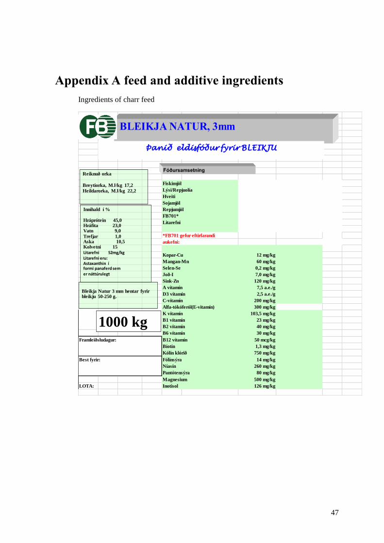
47

Appendix A feed and additive ingredients

Ingredients of charr feed

Fiskimjöl

Lýsi/Repjuolía

Hveiti

Sojamjöl

Repjumjöl

FB701*

Litarefni

*FB701 gefur eftirfarandi

aukefni:

Kopar-Cu 12 mg/kg

Mangan-Mn 60 mg/kg

Selen-Se 0,2 mg/kg

Joð-I 7,0 mg/kg

Sink-Zn 120 mg/kg

A vítamín 7,5 a.e./g

D3 vítamín 2,5 a.e./g

C-vítamín 200 mg/kg

Alfa-tókóferól(E-vitamín) 300 mg/kg

K vítamín 103,5 mg/kg

B1 vítamín 23 mg/kg

B2 vítamín 40 mg/kg

B6 vítamín 30 mg/kg

Framleiðsludagur: B12 vítamín 50 mcg/kg

Bíotín 1,3 mg/kg

Kólín klórið 750 mg/kg

Best fyrir: Fólínsýra 14 mg/kg

Níasín 260 mg/kg

Pantótensýra 80 mg/kg

Magnesium 500 mg/kg

LOTA: Inotisol 126 mg/kg

Þanið eldisfóður fyrir BLEIKJU

Innihald í %

Hráprótein 45,0 Hráfita 23,0 Vatn 9,0

Trefjar 1,0 Aska 10,5Kolvetni 15

Litarefni 52mg/kg Litarefni eru:Astaxanthin íformi panaferd semer náttúrulegt

Reiknuð orka

Breytiorka, MJ/kg 17,2

Heildarorka, MJ/kg 22,2

Bleikja Natur 3 mm hentar fyrir bleikju 50-250 g.

1000 kg

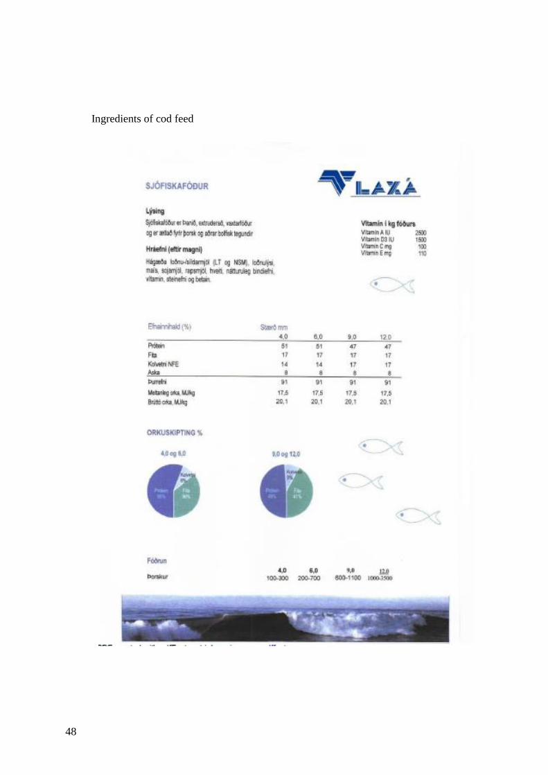
48

Ingredients of cod feed

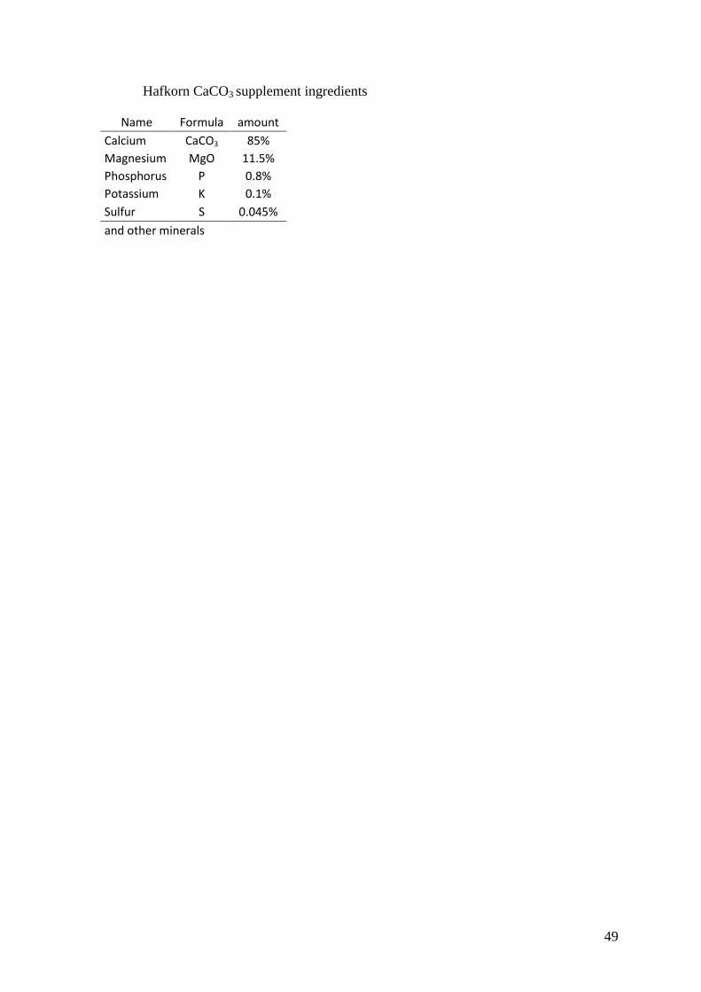
49

Hafkorn CaCO3 supplement ingredients

Name Formula amount

Calcium CaCO3 85%

Magnesium MgO 11.5%

Phosphorus P 0.8%

Potassium K 0.1%

Sulfur S 0.045%

and other minerals

50

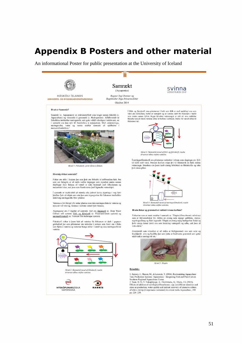
51

Appendix B Posters and other material

An informational Poster for public presentation at the University of Iceland

52

A poster for the Icelandic Biology conference 2015

53

Certificate of attendance in COST training school FA1305

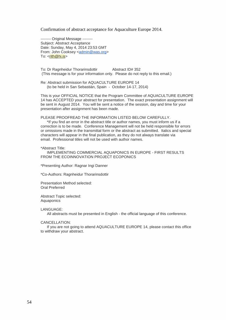
54

Confirmation of abstract acceptance for Aquaculture Europe 2014.

-------- Original Message -------- Subject: Abstract Acceptance Date: Sunday, May 4, 2014 23:53 GMT From: John Cooksey <admin@was.org> To: <rith@hi.is> To: Dr Ragnheidur Thorarinsdottir Abstract ID# 352 (This message is for your information only. Please do not reply to this email.) Re: Abstract submission for AQUACULTURE EUROPE 14 (to be held in San Sebastián, Spain - October 14-17, 2014) This is your OFFICIAL NOTICE that the Program Committee of AQUACULTURE EUROPE 14 has ACCEPTED your abstract for presentation. The exact presentation assignment will be sent in August 2014. You will be sent a notice of the session, day and time for your presentation after assignment has been made. PLEASE PROOFREAD THE INFORMATION LISTED BELOW CAREFULLY. *If you find an error in the abstract title or author names, you must inform us if a correction is to be made. Conference Management will not be held responsible for errors or omissions made in the transmittal form or the abstract as submitted. Italics and special characters will appear in the final publication, as they do not always translate via email. Professional titles will not be used with author names. *Abstract Title: IMPLEMENTING COMMERCIAL AQUAPONICS IN EUROPE - FIRST RESULTS FROM THE ECOINNOVATION PROJECT ECOPONICS *Presenting Author: Ragnar Ingi Danner *Co-Authors: Ragnheidur Thorarinsdottir Presentation Method selected: Oral Preferred Abstract Topic selected: Aquaponics LANGUAGE: All abstracts must be presented in English - the official language of this conference. CANCELLATION: If you are not going to attend AQUACULTURE EUROPE 14, please contact this office to withdraw your abstract.

55

Lecture schedule for a short course on aquaponics in June 2015

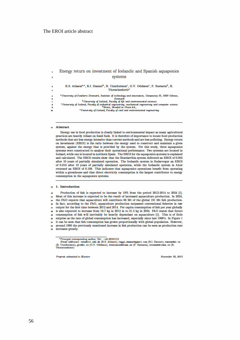
56

The EROI article abstract

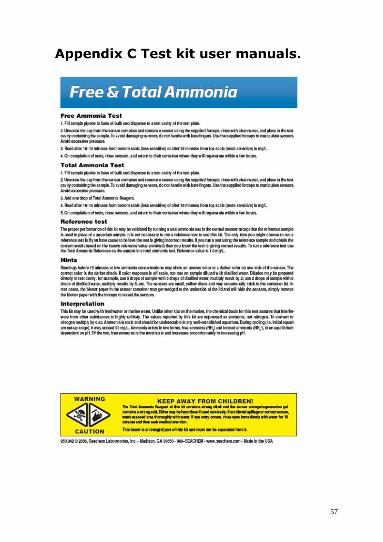
57

Appendix C Test kit user manuals.

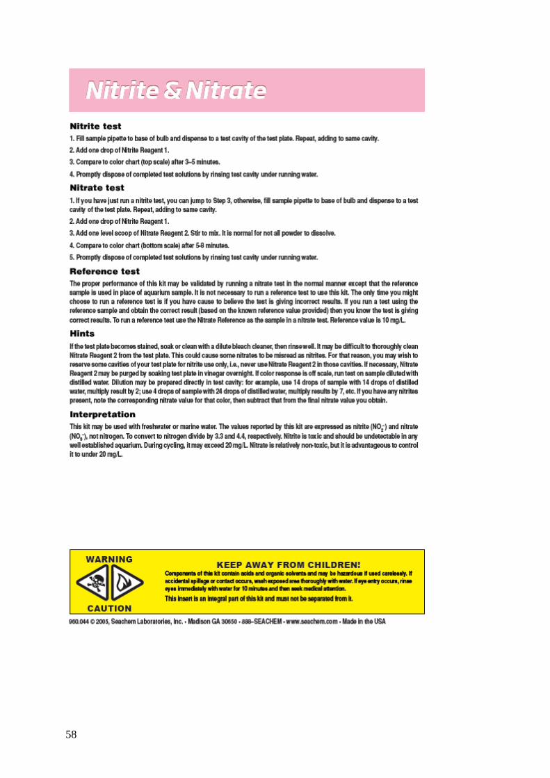
58

59