Designing and Performing BiologicalSolution Small-Angle Neutron ScatteringContrast Variation Experiments onMulti-component Assemblies

5

Susan Krueger

Abstract

Solution small-angle neutron scattering (SANS) combined with contrast

variation provides information about the size and shape of individual

components of a multi-component biological assembly, as well as the

spatial arrangements between the components. The large difference in the

neutron scattering properties between hydrogen and deuterium is key to

the method. Isotopic substitution of deuterium for some or all of the

hydrogen in either the molecule or the solvent can greatly alter the

scattering properties of the biological assembly, often with little or no

change to its biochemical properties. Thus, SANS with contrast variation

provides unique information not easily obtained using other experimental

techniques.

If used correctly, SANS with contrast variation is a powerful tool for

determining the solution structure of multi-component biological

assemblies. This chapter discusses the principles of SANS theory that

are important for contrast variation, essential considerations for experi-

ment design and execution, and the proper approach to data analysis and

structure modeling. As sample quality is extremely important for a suc-

cessful contrast variation experiment, sample issues that can affect the

outcome of the experiment are discussed as well as procedures used to

verify the sample quality. The described methodology is focused on

two-component biological complexes. However, examples of its use for

multi-component assemblies are also discussed.

Keywords

Small-angle neutron scattering • Contrast variation • Isotopic

substitution • Biological assemblies

S. Krueger (*)

NIST Center for Neutron Research, NIST, Gaithersburg,

MD 20899, USA

e-mail: susan.krueger@nist.gov

# Springer Nature Singapore Pte Ltd. 2017

B. Chaudhuri et al. (eds.), Biological Small Angle Scattering: Techniques, Strategies and Tips, Advancesin Experimental Medicine and Biology 1009, DOI 10.1007/978-981-10-6038-0_5

65

5.1 Introduction

Small-angle neutron scattering (SANS) is able to

provide the size, molecular mass and shape of a

macromolecular complex in solution on length

scales between approximately 10 Å to about

1,000 Å (Jacrot 1976; Svergun and Koch 2003;

Svergun 2010; Jacques and Trewhella 2010;

Zaccai 2012; Ankner et al. 2013). SANS com-

bined with contrast variation allows for the

unique retrieval of the internal structure and

organization of chemically distinct components

in a biological assembly. Recent reviews

(Neylon 2008; Whitten and Trewhella 2009;

Heller 2010; Gabel 2015; Zaccai et al. 2016) as

well as classic papers (Engelman and Moore

1975; Ibel and Stuhrmann 1975; Jacrot 1976)

describe the contrast variation technique as it

applies to biological systems in detail.

Contrast variation takes advantage of the large

difference in neutron scattering properties

between hydrogen and deuterium. By systemati-

cally varying the ratio of H2O to D2O (H2O:D2O

ratio) of the solvent, conditions are found in

which one component in a multi-component

assembly has the same scattering properties as

the solvent. Under these conditions, the

“matched” component is essentially invisible,

much like a transparent material, e.g., a glass

rod, can be optically invisible when in a solution

that matches its index of refraction. In theory, a

systematic series of measurements can be made

allowing the scattering from each component to

be determined as well as their positions with

respect to each other in the complex. Substitution

of deuterium for hydrogen in one or more of the

components of the complex is another form of

contrast variation.

This chapter introduces contrast variation

experiments, outlining pertinent principles of

SANS theory, essential considerations for exper-

iment design and execution, and the proper

approach to data analysis and structure modeling.

The discussions on experiment planning and

sample quality verification provide a guide for

preparing samples that will lead to a successful

contrast variation experiment. While the

methodology described here is focused on

two-component complexes, its use for multi-

component assemblies is also discussed.

5.2 Theory

5.2.1 Scattering Intensity

The measured SANS intensity from a macromol-

ecule consists of a coherent and an incoherent

contribution such that

I�~q� ¼ Icoh

�~q�þ Iinc: ð5:1Þ

The coherent contribution is dependent on the

scattering vector, ~q, which has a magnitude

defined as

q ¼ 4π sin θð Þλ

, ð5:2Þ

where 2θ is the scattering angle (typically in

degrees), measured from the axis of the incoming

neutron beam, and λ is the neutron wavelength.

The wavelength is usually expressed in nm or Å,such that q is stated in units of nm�1 or Å�1. The

shape of the coherent scattering intensity profile

depends on the shape of the molecule. On the

other hand, the incoherent contribution is not q-dependent and contributes mainly to the noise

level or “background”. Thus, the scattering inten-

sity will refer to only the coherent term unless

otherwise specified. The incoherent term will be

further discussed in the Experimental Method,

Data Analysis and Structure Modeling section.

Since SANS does not provide information on

the length scale of atomic bonds, the strength of

the scattering interaction can be described in

terms of a uniform scattering length density of

the entire molecule, ρ, within the molecular vol-

ume, V (in cm3 or Å3). The scattering length

density is usually expressed in units of cm�2 or

cm �3, but can be found stated in units of �2.

The SANS intensity from the molecule can be

written in terms of the scattering length density

as

66 S. Krueger

I�~q� ¼ ρ2V

1

V

ZV

ei~q�~rd~r����

����2

, ð5:3Þ

or

I�~q� ¼ ρ2V F

�~q��� ��2, ð5:4Þ

where F�~q��� ��2 is the form factor of the molecule.

5.2.2 Contrast

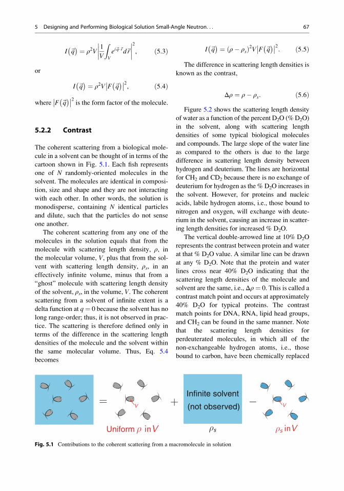
The coherent scattering from a biological mole-

cule in a solvent can be thought of in terms of the

cartoon shown in Fig. 5.1. Each fish represents

one of N randomly-oriented molecules in the

solvent. The molecules are identical in composi-

tion, size and shape and they are not interacting

with each other. In other words, the solution is

monodisperse, containing N identical particles

and dilute, such that the particles do not sense

one another.

The coherent scattering from any one of the

molecules in the solution equals that from the

molecule with scattering length density, ρ, in

the molecular volume, V, plus that from the sol-

vent with scattering length density, ρs, in an

effectively infinite volume, minus that from a

“ghost” molecule with scattering length density

of the solvent, ρs, in the volume, V. The coherent

scattering from a solvent of infinite extent is a

delta function at q¼ 0 because the solvent has no

long range-order; thus, it is not observed in prac-

tice. The scattering is therefore defined only in

terms of the difference in the scattering length

densities of the molecule and the solvent within

the same molecular volume. Thus, Eq. 5.4

becomes

I�~q� ¼ ρ� ρsð Þ2V F

�~q��� ��2: ð5:5Þ

The difference in scattering length densities is

known as the contrast,

Δρ ¼ ρ� ρs: ð5:6ÞFigure 5.2 shows the scattering length density

of water as a function of the percent D2O (%D2O)

in the solvent, along with scattering length

densities of some typical biological molecules

and compounds. The large slope of the water line

as compared to the others is due to the large

difference in scattering length density between

hydrogen and deuterium. The lines are horizontal

for CH2 and CD2 because there is no exchange of

deuterium for hydrogen as the % D2O increases in

the solvent. However, for proteins and nucleic

acids, labile hydrogen atoms, i.e., those bound to

nitrogen and oxygen, will exchange with deute-

rium in the solvent, causing an increase in scatter-

ing length densities for increased % D2O.

The vertical double-arrowed line at 10% D2O

represents the contrast between protein and water

at that % D2O value. A similar line can be drawn

at any % D2O. Note that the protein and water

lines cross near 40% D2O indicating that the

scattering length densities of the molecule and

solvent are the same, i.e., Δρ¼ 0. This is called a

contrast match point and occurs at approximately

40% D2O for typical proteins. The contrast

match points for DNA, RNA, lipid head groups,

and CH2 can be found in the same manner. Note

that the scattering length densities for

perdeuterated molecules, in which all of the

non-exchangeable hydrogen atoms, i.e., those

bound to carbon, have been chemically replaced

Uniform

(not observed)

Infinite solvent

Fig. 5.1 Contributions to the coherent scattering from a macromolecule in solution

5 Designing and Performing Biological Solution Small-Angle Neutron. . . 67

by deuterium, do not cross the water line. Thus,

the theoretical contrast match points for these

molecules would be greater than 100% D2O,

which is not obtainable in practice.

The SANS intensity from all N monodisperse,

randomly-oriented biological macromolecules in

a dilute solution can be written in terms of the

contrast as

I qð Þ ¼ n Δρð Þ2 V2 F�~q��� ��2D E

¼ n Δρð Þ2 V2P qð Þ, ð5:7Þ

where n is the number density (N per unit vol-

ume, v), of molecules (in cm�3). The brackets

represent an averaging over all orientations of the

molecule. The rotationally averaged form factor

is sometimes also called P(q). It can be seen fromEq. 5.7 that the scattering intensity is zero at the

contrast match point, Δρ ¼ 0.

A typical contrast variation experiment

involves measuring a complex consisting of two

components that have different scattering length

densities in solvent consisting of mainly water

with perhaps a small amount of salts and buffer-

ing compounds. When water mixtures with dif-

ferent H2O:D2O ratios are used, the contrast of

each component will change as a function of the

concentration of D2O in the solvent. Thus, con-

trast match points exist for each of the

components as well as the entire complex. As

the H2O:D2O conditions in the solvent are

varied, different parts of the complex scatter

more strongly depending on their individual scat-

tering length densities. By varying the amount of

D2O in the solvent, one component can be essen-

tially transparent at its contrast match point while

the others are still visible. If enough different

contrast conditions are measured, the scattering

intensities for the individual components as well

as their positions relative to each other are

obtained. It is this feature of SANS that makes

the method so powerful for selective measure-

ment of individual components within a

complex.

Fig. 5.2 Neutron

scattering length density as

a function of percentage

of D2O (% D2O) in the

solvent for some typical

biological molecules and

compounds (Zaccai et al.

2016)

68 S. Krueger

From Fig. 5.2, it is clear that proteins and

nucleic acids have different contrast match

points. The protein contrast match point is

around 40% D2O, meaning that only the DNA

or RNA is visible at this contrast. The DNA and

RNA contrast match points are around 65% D2O

such that only the protein is visible under these

conditions. Therefore, complexes consisting of

proteins and nucleic acids are ideal candidates

for contrast variation experiments (Gabel 2015).

For a complex consisting of two proteins,

replacement of some or all of the

non-exchangeable hydrogen atoms with deute-

rium in one of the components is required in

order for the two contrast match points to be

different. Since the contrast match point of

perdeuterated proteins is above 100% D2O, par-

tially deuterated proteins are generally used for

contrast variation experiments so that the con-

trast match point of the deuterated component is

somewhere between 60% D2O and 100% D2O

(Jacques et al. 2011). The exact contrast match

point of a deuterated component is dependent on

the amount of deuteration achieved. The contrast

variation experiment can be used to verify this

parameter, especially if a reliable determination

cannot be made by other methods such as NMR

or mass spectrometry. The method can be

extended to larger assemblies consisting of mul-

tiple copies of the two different components

(Appolaire et al. 2014).

Contrast variation methods also exist for solv-

ing the structures of multi-component assemblies.

The triple isotopic substitution method (TISM)

(Serdyuk and Zaccai 1996) allows for the deter-

mination of the scattering from one component at

a time. Each determination requires three

measurements with different deuteration levels

of the component of interest. The label triangula-

tion method (LTM) (Engelman and Moore 1972;

Hoppe 1973) allows for the structure of a complex

to be obtained by determining the distances

between pairs of components. Each distance

determination requires the selective labeling of

the two components of interest. After determining

a requisite number of distances, a 3D model of the

structure can be determined by triangulation. The

main applications of this method have been for the

determination of the location of various

components of the small (30S) and large (50S)

subunits of the ribosome. These historic works are

referenced in (May and Nowotny 1989).

Both the TISM and LTM methods require a

large number of measurements. In practice,

measurements of complexes consisting of three

or more components are often made under sol-

vent conditions that match each of the individual

components. While some components still must

be deuterated, this approach limits the number of

measurements needed. An attempt is then made

to find model structures that best fit all of the

contrast variation data. This approach often

works well when atomistic level starting

structures of individual components are already

available or can be built using homology

modeling techniques, distance constraints are

available from other techniques and/or docking

software can be used to build structure models.

The value of any such model is determined by its

ability to reproduce the SANS data.

5.2.3 Radius of Gyration and ForwardScattering Intensity

The radius of gyration, Rg, which is similar to the

moment of inertia with respect to the scattering

center of mass, and the forward scattering inten-

sity, I(0), which is the scattering intensity at q¼ 0,

are two important model-independent parameters

that are obtained from SANS data. Rg provides

information about the size of the molecule

whereas I(0) provides information about its

molecular weight. Both parameters depend on

the contrast, which can provide important clues

about the spatial distribution of contrast within the

molecule.

By definition, P(q) in Eq. 5.7 is equal to 1 at

q ¼ 0. Thus,

I 0ð Þ ¼ n Δρð Þ2 V2: ð5:8ÞThe number density, n (cm�3), can be written

in terms of the concentration of the molecule,

c (g cm�3), as

5 Designing and Performing Biological Solution Small-Angle Neutron. . . 69

n ¼ cNA

Mw, ð5:9Þ

where Mw is the molecular weight of the mole-

cule (in Da, where 1 Da ¼ 1 g mole�1) and NA is

Avogadro’s number. In addition, the molecular

volume, V, can be written in terms of the partial

specific volume, �v (cm3 g�1), as

V ¼ �vMw

NA: ð5:10Þ

Equations 5.8, 5.9 and 5.10 can be used to

relate I(0) to the Mw of the molecule if the

SANS data are on an absolute scale, usually in

units of cm�1. While I(0) ¼ 0 at the contrast

match point, this is not true at larger angles that

correspond to length scales on the order of the

internal scattering length density fluctuations that

were ignored by assuming a uniform scattering

length density in Eq. 5.3.

The Guinier approximation (Guinier and

Fournet 1955),

I qð Þ ¼ I 0ð Þ exp �q2R2g

3

!, ð5:11Þ

can be used on the low-q portions of the data to

obtain values for Rg and I(0). This low-q analysis

is valid only in the region where qRg ≲ 1.3, so

the valid q range depends on the size of the

molecule. A shape must be assumed for the mol-

ecule to relate Rg to the molecular dimensions. Rg

and I(0) are found by plotting the natural log of

Eq. 5.11 such that

ln I qð Þð Þ ¼ ln I 0ð Þð Þ � q2R2g

3: ð5:12Þ

A linear fit of ln(I(q)) vs q2 (Eq. 5.12) to

the low-q portion of the data allows the determi-

nation of Rg from the slope and I(0) from the

intercept.

Another method to obtain Rg and I(0), whichmakes use of all of the data rather than a limited

data set at small q values, is to use the distance

distribution function, P(r) vs r (Glatter and

Kratky 1982). This function represents the prob-

ability distribution of distances, r, between all

pairs of atoms in the molecule. The result is a

smooth histogram-like plot with peaks at the

most probable distances in the molecule. Thus,

the shape of the P(r) vs r curve depends stronglyon the shape of the molecule and can vary as a

function of contrast.

P(r) is typically obtained from the SANS data

using an indirect Fourier transformation method

(Glatter 1977; Moore 1982; Semenyuk and

Svergun 1991) using the relation

I qð Þ ¼ 4πV

Z Dmax

0

P rð Þ sin qrð Þqr

dr: ð5:13Þ

This analysis requires a stipulation by the user

of a maximum dimension, Dmax, beyond which P

(r) ¼ 0. Typically, several values of Dmax are

explored in order to find the range over which

the P(r) function doesn’t change as a function of

Dmax. Typically, the condition that P(r) ¼ 0 at

r ¼ 0 is also assumed. Rg and I(0) can be derivedfrom P(r), as described in (Glatter 1982).

5.3 Experimental Method, DataAnalysis and StructureModeling

The successful SANS contrast variation experi-

ment requires a number of steps from experiment

planning and sample preparation to data collec-

tion and analysis, culminating with structure

modeling. A flow chart showing these different

steps is shown in Fig. 5.3 and each is described in

detail in this section.

5.3.1 Sample Considerations

To obtain the most information possible from a

contrast variation experiment, the main require-

ment is that the biological complex must be

measured under dilute and monodisperse

conditions in all H2O:D2O solvents. In other

70 S. Krueger

words, the sample must be of high purity. Ideally,

this means that all the molecules have the same

stoichiometry under all contrast conditions and

there are no “free” components in the solution.

Furthermore, all of the complexes are in identical

conformations and there are no interactions

between the complexes. The above equations

describing the scattering intensity from

macromolecules in solution assume these

conditions are met.

In practice, there are many reasons why a

sample might not meet all of these conditions.

Sample preparation for contrast variation

experiments involves making biological

complexes in solvents containing D2O. In some

cases, the complexes themselves must be made

using deuterated components, which is typically

accomplished by expressing one of the protein

components using bacteria grown in deuterium-

enriched media.

Whenever deuterium is introduced into the

molecule or solvent, there is an increased chance

for undesirable aggregation, even under

conditions where the complex would not aggre-

gate were deuterium absent. SANS is a volume-

weighted technique. Since larger aggregates have

larger volumes, a small amount of larger

aggregates contribute more to the scattering

intensity than a larger amount of small

aggregates. While the signature of aggregation

is most obvious at lower q values, the contribu-

tion to the total scattering persists over a much

wider q range. Another issue when using

deuterated components is that the complex

might not form as readily or stably. This can

lead to a situation for which the complex is

associating and dissociating at a constant rate.

In such situations, it may not always be possible

to avoid having an excess of the constituent

components in the solution.

The amount of sample needed for a contrast

variation experiment is on the order of 0.5 mL at

a concentration of 1–5 mg mL�1 for complexes

with a typical Mw between 50 and 100 kDa.

Under solvent conditions where the contrast,

and thus I(q) is low, higher concentrations must

sometimes be used. This may introduce interpar-

ticle interference or aggregation effects that need

to be mitigated as much as possible, e.g., by

adding salts to the solvent to screen electrostatic

interactions or by adding compounds that inhibit

hydrophobic interactions. The mitigation of

interparticle interference and aggregation effects

is a difficult problem since every complex is

different and measures that work in one case

may not work in another.

Given the amount of material needed for a

contrast variation experiment, the care that must

be taken to prepare the samples, and the cost and

time involved in getting access to a SANS

beamline, it is important that such experiments

are well planned and that these issues are consid-

ered and tested well before committing to

making samples for a complete set of contrast

variation measurements. Steps that can be taken

to insure sample purity are discussed in detail in

(Jacques and Trewhella 2010). Thorough sample

characterization under the conditions that are

Fig. 5.3 Flow chart showing the steps necessary for performing a successful SANS contrast variation experiment

5 Designing and Performing Biological Solution Small-Angle Neutron. . . 71

being used for SANS should be performed prior

to the SANS experiments using not only bio-

chemical assays such as SDS-PAGE and gel

filtration, but also complementary physical char-

acterization techniques such as size exclusion

chromatography with multi-angle light scattering

(SEC-MALS), dynamic light scattering (DLS),

or analytical ultracentrifugation (AUC). The

amount of deuteration in a deuterated component

can be assessed by mass spectroscopy or deute-

rium NMR. Small-angle X-ray scattering

(SAXS) measurements can also be very helpful

to detect concentration or D2O-dependent aggre-

gation as will be discussed in more detail below.

5.3.2 Experiment Planning

For two component systems, the contrast of each

component as well as that for the complex can be

calculated from the chemical composition of

each component and the stoichiometry of the

complex as a function of the solvent composi-

tion. Two applications for performing this calcu-

lation are the MULCh (Whitten et al. 2008)

software and the Contrast Calculator (Sarachan

et al. 2013) module of the SASSIE (Curtis et al.

2012) software. For proteins and nucleic acids,

the chemical composition is defined in terms of

the amino acids or nucleotide bases, respectively,

including the amount of H-D exchange and deu-

teration for each component. Non-protein or

nucleic acid components can be entered based

on their chemical formulas. Non-water solvent

components such as salts and buffering

compounds can be included in the calculation

of the solvent scattering length densities to deter-

mine if they significantly alter the contrast match

points. This is usually not the case if they are

present in typical mmoles L�1 (mM) quantities.

Both contrast calculating programs provide a

web interface for easy access and use. While

MULCh is limited to two-component complexes,

it also provides options for data analysis that will

be described further below. The Contrast Calcu-

lator module allows for an unlimited number of

components in the complex and additionally

calculates expected I(0) values as a function of

solvent composition. The predicted I(0) values

are invaluable in determining the concentration

needed to obtain a measurable signal for each

solvent condition. If atomic coordinates are

available, such as from X-ray crystallography or

NMR structures, model scattering intensity

curves can be calculated at each contrast to per-

form the SANS experiment in silico prior to the

actual experiment. Software such as CRYSON

(Svergun et al. 1998) or the SasCalc (Watson and

Curtis 2013) module of SASSIE can be used for

this purpose. The experimental SANS data may

not match that calculated from the model struc-

ture if, for instance, disordered residues are miss-

ing or if the structure doesn’t accurately

represent the complex in solution. Model

structures must be complete if they are to be

used as starting points for further modeling

once SANS data are obtained. Thus, missing N

or C terminal residues, internal loops, domains

and/or disordered linkers must be added if

necessary.

The calculations of the scattering length

densities, contrast, I(0) and model scattering

intensity curves used to plan an experiment

apply only to the coherent scattering component

in Eq. 5.1. The hydrogen and deuterium in the

biological complex also have an incoherent scat-

tering component, which contributes a small

amount to the total scattering in dilute solutions.

On the other hand, the incoherent scattering from

a solvent containing mostly H2O:D2O is signifi-

cant. In fact, it can often be greater than the

calculated coherent intensity of a typical com-

plex in a dilute solution. For example, the calcu-

lated coherent I(0) value for a 1 mg mL�1

protein-protein complex consisting of a trimer

of the chaperone, Skp, bound to 50% deuterated

outer membrane protein, OmpA, is 0.086 cm�1

in H2O (i.e., 0% D2O) and 0.04 cm�1 in 98%

D2O (Sarachan et al. 2013). However, the inco-

herent scattering intensity for 98% D2O

is � 0.07 cm�1 and that of H2O is � 1.0 cm�1

(Rubinson et al. 2008). Thus, the incoherent

component is the dominant contributor to the

total scattering in H2O, and remains a significant

contributor in 98% D2O.

72 S. Krueger

The calculated scattering curves for the

Skp-OmpA complex are shown in Fig. 5.4 with

and without the addition of the incoherent scat-

tering component. The scattering that is actually

measured is that shown in Fig. 5.4b. Under ideal

conditions where there are no error bars on the

data points in Fig. 5.4b and the incoherent back-

ground is measured equally well, the scattering

curves in Fig. 5.4a could be recovered. However,

this is not the case in practice. Features such as

that shown at q � 0.2 �1 for the complex in

H2O (Fig. 5.4a) generally are not observable in

practice since the incoherent component already

significantly influences the total scattering at

q � 0.1 �1 (Fig. 5.4b). On the other hand,

features such as those shown at 0.15 �1 �q � 0.25 �1 for the complex in 98% D2O

typically are observable after subtraction of the

incoherent scattering component. This subtrac-

tion is accomplished by measuring the incoherent

scattering from a solvent that matches that of the

sample as closely as possible. Thus, dialysis is an

ideal method for exchanging the biological com-

plex into buffers with different H2O:D2O ratios,

as the dialysate solution can then be used to

measure the incoherent background scattering.

The incoherent scattering from the solvent

must be considered when planning data collec-

tion times. For a given calculated coherent I

(0) value, it will take longer to obtain data in

H2O than in D2O if the data are to have similar

statistics after the incoherent background is

subtracted. Furthermore, since the incoherent

background is much higher in H2O, the maxi-

mum q value obtained after buffer subtraction

will be lower for data obtained in H2O. Thus,

when planning an experiment, samples prepared

in solvents containing less than 50% D2O often

must be measured a higher concentration so that

the coherent I(0) is higher to make up for the

higher incoherent background under these

conditions. It should be noted that the scattering

from water can contain both incoherent multiple

scattering and inelastic scattering contributions

and thus can differ depending on instrument

conditions and sample geometry (Carsughi et al.

2000; Rubinson et al. 2008; Do et al. 2014). As

the instrument scientists are most familiar with

their instruments, it is important to rely on their

advice for the I(0) values that can reasonably be

measured at a given contrast at their facility.

Prior to performing a series of contrast varia-

tion measurements, two series of sample

a b

Fig. 5.4 Calculated I(q) values for a Skp-OmpA com-

plex in H2O (i.e., 0% D2O) and 98% D2O solvents (a)without incoherent scattering and (b) with incoherent

scattering. The coherent scattering curves were calculated

using the SasCalc module in SASSIE

5 Designing and Performing Biological Solution Small-Angle Neutron. . . 73

concentrationmeasurements should be performed,

one in H2O and one in >95% D2O, to determine

themaximum concentration at which the sample is

dilute and monodisperse. These measurements

also identify whether there are any effects due to

the presence of D2O in the solvent. Discussions

with instrument scientists, who are familiar with

the range of I(0) values that are measurable at their

facility, provide the best resource in planning the

range of sample concentrations to examine. This

will avoid wasting time measuring the complex at

sample concentrations that would result in

I(0) values that are too low to be measured. It

should also be noted that the accuracy of the

concentration is extremely important, as it is the

main source of error for determining theMw from

I(0) (Eqs. 5.8 and 5.9).

The SANS curves from a complex often are

significantly different in H2O and D2O solvents.

Indeed, this is the reason for performing a contrast

variation experiment in the first place. Therefore,

the measurements described above are for com-

parison of the behavior of the complex as a func-

tion of concentration separately in H2O and

D2O. The concentration needed to satisfy the

dilute and monodisperse conditions may be

lower in D2O than in H2O. If a SAXS instrument

is available, SAXS measurements are a good

option to determine whether there are any effects

from either deuterium in the complex (when it

consists of a deuterated and non-deuterated pro-

tein, for example) or D2O in the solvent. Since

X-rays are not sensitive to the difference between

hydrogen and deuterium, the scattering curves

should ideally be the same regardless of sample

or solvent deuteration. Another advantage is that

SAXS measurements require smaller samples, on

the order of 50 μL, requiring less sample prepara-

tion time for these important feasibility

measurements. The SAXS measurement can also

serve as another contrast point that can assist in

modeling the structure of the complex.

Once optimal concentrations in H2O and D2O

solvents have been found, then the feasibility of

performing the contrast variation experiment can

be further assessed by referring back to the

predicted I(0) values obtained for the complex

as a function of D2O in the solvent. For instance,

is there a conflict between the concentration

needed to obtain a reasonable signal and that

needed to obtain a dilute and monodisperse sam-

ple at a given solvent condition? Is there a way to

mitigate the issue, perhaps by altering the solvent

conditions slightly? Again, an experienced

instrument scientist can be a valuable resource

when considering these types of issues.

5.3.3 Data Collection and Reductionto I(q) vs q

Data collection consists of measuring both the

transmission of neutrons through the sample and

the scattering of neutrons from the sample. Typi-

cally, these two different types of measurements

require different instrument configurations and are

performed separately. Since the sample consists of

a biological complex in a solvent, these same

measurements are also made for the solvent

alone. Recall from Fig. 5.1 that the coherent scat-

tering from the solvent is not observable. How-

ever, Fig. 5.4b shows that the incoherent scattering

from a solvent containing mostly H2O:D2O is sig-

nificant and therefore must be subtracted from the

total sample scattering, which also contains this

incoherent component from the solvent. Since

both the sample and solvent alone are measured

in a sample holder, often a quartz cuvette or a

demountable cell with quartz windows, the trans-

mission and scattering from the empty holder (i.e,

the empty cell) should also be measured.

Typical windows used for SANS such as

quartz, aluminum and titanium have significant

scattering in the forward direction. Subtracting

the scattering of the empty cell from both the

sample and the solvent alone will eliminate the

scattering contribution from the windows so that

the shape of the scattering from the sample and

solvent can be accurately observed. The solvent

scattering should then be approximately flat since

it is mainly incoherent and, hence, not q-depen-dent (Eq. 5.1). Furthermore, the scattering

observed from the sample is then attributed to the

biological complex of interest plus the solvent

(as in Fig. 5.4b) with no contribution from the

sample holder. The transmission measurement is

74 S. Krueger

important for proper subtraction of the empty cell

and for placing the data on an absolute scale as

described, for example, in (Glinka et al. 1998).

An additional consideration when collecting

data is the time spent measuring each sample.

Counting times for transmission measurements

from the sample, solvent and empty cell are typi-

cally just a few minutes. On the other hand,

counting times for scattering measurements from

the sample (complex plus solvent) are concentra-

tion, contrast and instrument dependent and

should be determined in consultation with the

instrument scientist. For dilute samples, the

counting statistics on the sample and solvent

alone should be equivalent since the incoherent

scattering from the solvent dominates the total

scattering at most q values measured (Fig. 5.4).

Thus, counting times for the sample and solvent

alone should be the same. This is especially criti-

cal for measurements made under low contrast

conditions. An exception can sometimes be

made for a highMw complex, or for measurements

made under high contrast conditions, if the scat-

tering is significantly higher than that of the sol-

vent alone in the low-q region of the I(q) vs

q curve. However, the counting statistics of the

sample and solvent scattering should still be equal

in the higher-q portion of the curves, where the

signal from the complex is weak. Since the empty

cell scatters predominately in the forward direc-

tion, the counting times for these measurements

can be shorter, matching only the statistics of the

sample in the low-q region.

In a dilute solution, the incoherent scattering

from the hydrogen and deuterium in the

biological complex itself is negligible compared

to that from the solvent. While the background

levels of both sample and solvent alone should be

the same in this case, mismatches can occur for a

variety of reasons. Some possible sources for

these mismatches include statistical differences

in transmission values, the influence of incoher-

ent multiple scattering, micro- or macroscopic

bubbles in the solution, and mismatch in H2O:

D2O ratio between the sample and solvent alone.

However, under dilute conditions, the incoherent

scattering from the solvent alone can be removed

by scaling it to match the high-q region of the

total sample scattering and then subtracting

it. The acceptability of the solvent subtraction

can be assessed by not requiring that P(r) ¼ 0 at r ¼ 0 when calculating P(r) from the

SANS data (Jacques and Trewhella 2010). If P

(0) is positive or negative, then the solvent has

been under- or over-subtracted, respectively.

This approximation, used to remove the solvent

scattering by scaling it to match the sample scat-

tering, does not apply to concentrated solutions

(concentrations � 10 mg mL�1 and above for

samples in a D2O buffer), where the incoherent

scattering from the non-exchangeable hydrogen

atoms in the complex itself is significant. As an

alternative, it is tempting to simply subtract a

constant representing the incoherent scattering

from the solvent rather than subtract the measured

scattering from the solvent alone, but this only

works if the scattering from the solvent is truly

flat. Typically the solvent scattering is not exactly

flat due to incoherent multiple scattering, inelastic

scattering, and other contributions(Carsughi et al.

2000; Rubinson et al. 2008; Do et al. 2014), with

the shape depending on the H2O:D2O conditions

of the solvent. Given these issues, in practice it is

quite difficult to accurately subtract the solvent

scattering from the sample scattering. Thus, it is

not uncommon to find a systematic background

mismatch when comparing the calculated SANS

curves to the measured SANS data during the

structure modeling stage.

Methods of reducing data from the raw data

collected on a 2D position-sensitive detector to

the 1D I(q) vs q data vary depending on the

facility. However, if the end result is a set of

separate I(q) vs q curves on an absolute scale

for both the sample and the solvent alone, the

scattering from the solvent can be successfully

subtracted. If the solvent subtraction is

performed as part of the 2D data reduction, then

it is more difficult to diagnose problems that

often arise during the solvent subtraction step.

5 Designing and Performing Biological Solution Small-Angle Neutron. . . 75

5.3.4 Data Quality Checks

5.3.4.1 Rg and I(0)Once contrast variation data have been reduced

and the contribution from the solvent has been

subtracted, the basic parameters, Rg and I(0)

should be obtained at all contrasts using both

the Guinier and P(r) analyses (Eqs. 5.11–5.13).

Guinier analysis is usually provided by scattering

facilities as part of the data reduction software. If

P(r) analysis isn’t also included, a program such

as GNOM (Semenyuk and Svergun 1991) or

BayesApp (Hansen 2014) can be used. The

experimental values of I(0) are then compared

to the calculated values at each contrast in order

to confirm the integrity of the samples. The num-

ber density, n, is defined as in Eq. 5.9, but it is

now in terms of the concentration and Mw of the

entire complex. Similarly, Δρ refers to the mean

contrast of the entire complex and V is the vol-

ume of the complex. The Mw values should

match the calculated values to within 10% if the

data are on an absolute scale, I(0) has an error of

1-2%, and the concentrations are measured to

within 5%.

If the solution consists of a mixture of

monomers and dimers of the complex or another

combination of low-order oligomers, a valid

Guinier region may still exist, but the I(0) value

will be larger than that of the monomeric com-

plex. If there are larger aggregates of the mole-

cule in the solution, the Guinier region will occur

at smaller q values than expected and Eq. 5.12

will not be linear in the q-range related to the

expected size of the complex. Rather it will have

some curvature and the fit to a straight line in the

expected q-range will be poor. The effects can be

subtle or very obvious depending on the severity

of the aggregation (Jacques and Trewhella 2010).

If aggregation is present, whether subtle or

severe, the Rg and I(0) values no longer represent

that of a monomer complex in a monodisperse

solution. Rather, they are influenced by the larger

aggregates present in the solution. The P(r) func-

tion also changes in response to aggregation,

primarily in the high-r region. In cases of minor

aggregation, it may still be possible to calculate a

P(r) corresponding to the monomer but the more

severe the aggregation, the more difficult it is to

determine Dmax (Jacques and Trewhella 2010).

5.3.4.2 Contrast Match Point AnalysisTo further confirm the integrity of the sample at

all contrasts, the contrast match point of the of

the complex can be determined from the experi-

mental data. Expanding on Eqs. 5.8–5.10I(0) canbe written in terms of a two-component complex

as,

I 0ð Þ ¼ cMw

NA

�f 1Δρ1�v1 þ f 2Δρ2�v2

�2, ð5:14Þ

where f1 and f2 are the respective mass fractions

of the first and second components in the com-

plex. Now, Δρ1 and Δρ2 are respectively the

scattering contrasts of the first and second

components and �v1 and �v2 are respectively the

partial specific volumes of the first and second

components (Sarachan et al. 2013).

Because I(0) is proportional to c and to (Δρ)2,which is in turn dependent on the fraction of D2O

in the solvent, fD2O, the contrast match point of

the complex can be determined from the

x-intercept of a linear fit toffiffiffiffiffiffiffiffiffiffiffiI 0ð Þ=c

pvs fD2O

. An

example of this analysis is shown in Fig. 5.5,

where experimental values offfiffiffiffiffiffiffiffiffiffiffiI 0ð Þ=c

pvs fD2O

are plotted for the aforementioned Skp-OmpA

complex that was measured in 0%, 15%,

30% and 98% D2O buffer. An unweighted

linear fit to the data resulted in a line with a

slope of �0.51 � 0.01 and a y-intercept of

0.294 � 0.006, where the errors represent one

standard deviation. The x-intercept corresponding

to the match point of the complex was calculated

to be 0.576 � 0.014, or 57.6% � 1.4% D2O.

This analysis can also be performed using

MULCh (Whitten et al. 2008) and requires the

experimental I(0) values, the concentration of the

complex and the fraction of D2O in the buffer at

each contrast.

Comparison of this experimentally deter-

mined contrast match point to that calculated

with Δρ1 and Δρ2 determined from the chemical

composition of each component provides another

quality assurance test on the data in that the

76 S. Krueger

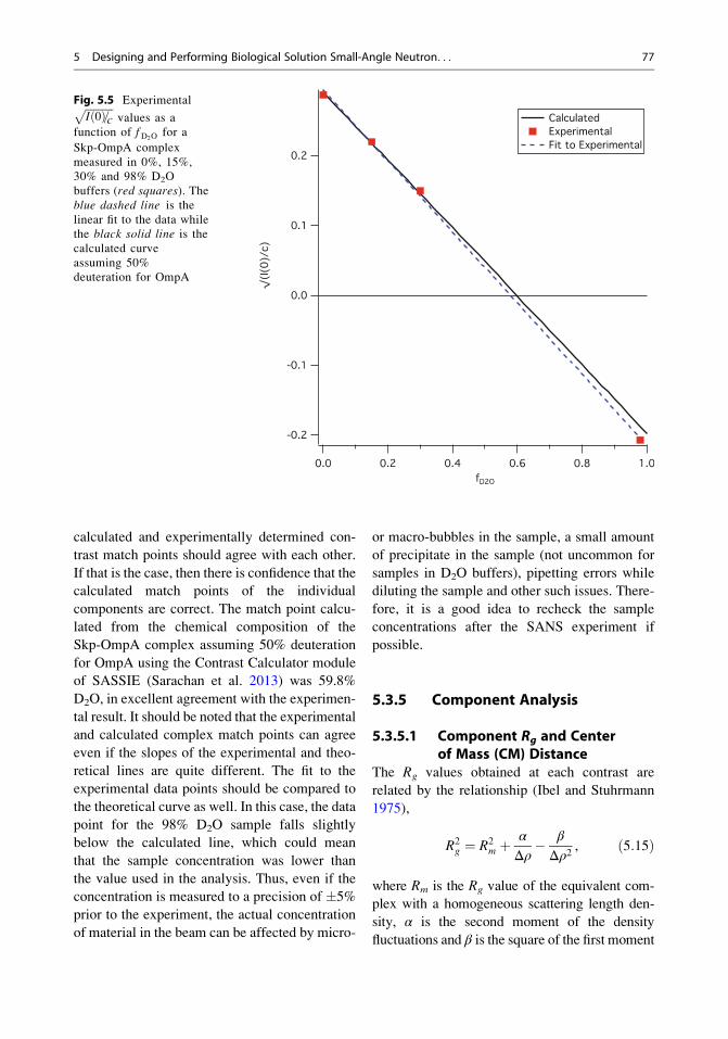
calculated and experimentally determined con-

trast match points should agree with each other.

If that is the case, then there is confidence that the

calculated match points of the individual

components are correct. The match point calcu-

lated from the chemical composition of the

Skp-OmpA complex assuming 50% deuteration

for OmpA using the Contrast Calculator module

of SASSIE (Sarachan et al. 2013) was 59.8%

D2O, in excellent agreement with the experimen-

tal result. It should be noted that the experimental

and calculated complex match points can agree

even if the slopes of the experimental and theo-

retical lines are quite different. The fit to the

experimental data points should be compared to

the theoretical curve as well. In this case, the data

point for the 98% D2O sample falls slightly

below the calculated line, which could mean

that the sample concentration was lower than

the value used in the analysis. Thus, even if the

concentration is measured to a precision of �5%

prior to the experiment, the actual concentration

of material in the beam can be affected by micro-

or macro-bubbles in the sample, a small amount

of precipitate in the sample (not uncommon for

samples in D2O buffers), pipetting errors while

diluting the sample and other such issues. There-

fore, it is a good idea to recheck the sample

concentrations after the SANS experiment if

possible.

5.3.5 Component Analysis

5.3.5.1 Component Rg and Centerof Mass (CM) Distance

The Rg values obtained at each contrast are

related by the relationship (Ibel and Stuhrmann

1975),

R2g ¼ R2

m þ α

Δρ� β

Δρ2, ð5:15Þ

where Rm is the Rg value of the equivalent com-

plex with a homogeneous scattering length den-

sity, α is the second moment of the density

fluctuations and β is the square of the first moment

Fig. 5.5 ExperimentalffiffiffiffiffiffiffiffiffiffiffiI 0ð Þ=c

pvalues as a

function of fD2Ofor a

Skp-OmpA complex

measured in 0%, 15%,

30% and 98% D2O

buffers (red squares). Theblue dashed line is the

linear fit to the data while

the black solid line is the

calculated curve

assuming 50%

deuteration for OmpA

5 Designing and Performing Biological Solution Small-Angle Neutron. . . 77

of the density fluctuations. For two component

systems with different scattering length densities,

the term α relates to the distribution of scattering

length densities relative to the center of mass

(CM) of the complex, and the term β provides

the separation of the scattering CM of the two

components (Moore 1982). A Stuhrmann plot

(Ibel and Stuhrmann 1975) of R2g vs (Δρ)�1

(Eq. 5.15) is used to determine Rm, α, and β. Ifthe plot is linear, then β¼ 0 and the CM of the two

components are concentric. In this case, the sign

of the slope of the line, α, is an indication of

whether the component with the higher scattering

length density is on the interior (negative) or exte-

rior (positive) of the complex. Examples of para-

bolic and linear Stuhrmann plots are shown in

Fig. 5.6. In practice, it is not always easy to

distinguish between a parabolic and linear

Stuhrmann plot, especially if Rg doesn’t change

appreciably as a function of contrast (α is close to

zero) or if Rg values are not available close to the

individual contrast match points of the two

components.

Similar information can be obtained from the

parallel axis theorem

R2g ¼

Δρ1 V1

ΔρVR21 þ

Δρ2 V2

ΔρVR22

þ Δρ1 Δρ2 V1 V2

ΔρVð Þ2 D2CM, ð5:16Þ

where R1 and R2 are the radii of gyration of the

components and DCM is the distance between the

scattering CM of the two components (Engelman

and Moore 1975). Here, Δρ1, Δρ2, V1 and V2

refer to the individual components and Δρ and

V refer to the complex. The parallel axis theorem

provides the radii of gyration of the components

and the CM distance between them directly,

whereas they are calculated from the definitions

of α and β when the Stuhrmann analysis is used.

In both cases, R1, R2 and DCM are contrast-

independent values that can be used in the struc-

ture modeling process. The MULCh software

provides both of these analyses (Whitten et al.

2008). The inputs are the measured Rg values as a

function of fD2O in the solvent. The contrasts,Δρ,Δρ1 and Δρ2, are determined from the chemical

composition of each component based on the

sequence information input earlier in the

analysis.

a b

Fig. 5.6 Examples of Stuhrmann plots from a

two-component complex in which a the centers of mass

are not concentric and b the centers of mass are

concentric and the component with the higher scattering

length density is on the exterior of the complex

78 S. Krueger

5.3.5.2 Component ScatteringIntensities and Cross-Term

The scattering intensity from a two-component

system with different scattering length densities

can be written as (Whitten et al. 2008)

I qð Þ ¼ Δρ12 I1 qð Þ þ Δρ1Δρ2I12 qð Þþ Δρ2

2 I2 qð Þ, ð5:17Þ

where I1(q) and I2(q) are the scattering intensities

of components 1 and 2, respectively, and I12(q) is

the scattering intensity due to the interference

between the two components. I1(q) and I2(q) are

related to the shapes of the two components and

I12(q) is related to their spatial distribution. For a

given set of measured contrast variation

intensities, I(q), and known values for the

contrasts, Δρ1 and Δρ2, the three unknowns,

I1(q), I2(q) and I12(q), are found by solving the

resultant set of linear equations at each q value.

Thus, data must be obtained at a minimum of

three contrasts to solve for the three unknowns.

The MULCh software (Whitten et al. 2008)

provides this analysis. The measured I(q) vs

q SANS curves and complex concentrations are

required for each contrast and Δρ1 and Δρ2 are

determined from the chemical composition of

each component based on the sequence informa-

tion input earlier in the analysis.

In practice, successful contrast variation stud-

ies that have resulted in the determination of

I1(q), I2(q) and I12(q) have employed at least

five strategically chosen contrast points includ-

ing the contrast match points of the individual

components, where high quality data were

obtained (Whitten et al. 2008). An example of a

successful application of this method can be

found in a study of a kinase, KinA, in complex

with an inhibitor, Sda (Whitten et al. 2007).

Based on this study and an analysis of the

corresponding theoretical scattering curves with

noise added, a data collection strategy was

recommended that includes a minimum of two

contrast points on either side of the average

match point of the entire complex (Whitten

et al. 2008). This results in a well-spread range

of contrast points that allows the individual R1,

R2 and DCM to be obtained with good accuracy

and precision.

For a complex consisting of a protein and

nucleic acid or a protein and a deuterated protein

(with a deuteration level such that the match

point is between 60% D2O and 80% D2O), a

typical contrast variation data set would include

0% D2O and 100% D2O, along with 20% D2O,

40% D2O (the protein match point) and a fifth

contrast point between 70% D2O and 80% D2O

(near the match point of the second component).

To obtain accurate scattering intensities of the

components (Eq. 5.17), high quality data are

needed at all measured contrasts. This analysis

can be a useful tool to model the components

separately and then arrange them with respect to

each other in their proper position within the

complex. However, structure modeling can pro-

ceed on the basis of the individual R1, R2 and

DCM information alone, as is shown by example

below.

5.3.6 Structure Modeling

Both SAXS and SANS are being used for struc-

tural determination of large biological complexes

and for complexes containing flexible regions in

solution. Many options are available for

modeling multimeric biological complexes

using a combination of rigid body and atomistic

approaches, as described in recent reviews

(Putnam et al. 2007; Rambo and Tainer 2010;

Schneidman-Duhovny et al. 2012; Boldon et al.

2015). The SASSIE software suite (Curtis et al.

2012) is one tool that is available to assist in the

atomistic and rigid body structure modeling of

biological molecules for comparison to SAXS

and SANS data. SASSIE provides users access

to molecular dynamics, Monte Carlo, docking

and rigid body modeling methods to assist in

generating structure models and assessing how

well models match the data. Constraints can be

incorporated from other techniques such as NMR

and AUC. SASSIE has been used for the struc-

ture modeling of many biological systems,

including intrinsically disordered monomeric

proteins (Curtis et al. 2012), large protein

5 Designing and Performing Biological Solution Small-Angle Neutron. . . 79

complexes (Krueger et al. 2011, 2014) and

single-stranded nucleic acids (Peng et al. 2014).

It has also been applied to the study of monoclo-

nal antibodies using free energy analysis (Clark

et al. 2013). A web version is available (https://

sassie-web.chem.utk.edu/sassie2/) for ease of

access and to handle the intensive computational

requirements of the structural modeling and data

analysis.

For a two-component complex, SANS and

contrast variation experiments provide the

added structural information from the individual

components as constraints for modeling the

entire complex. If obtainable, the scattering

intensities of the separate components

(Eq. 5.17) can be helpful for the modeling of

the individual components and for construction

of the model structure for the entire complex

(Whitten et al. 2008). However, the contrast-

independent R1, R2 and DCM distance constraints

found by the Stuhrmann (Eq. 5.15) and parallel

axis theorem (Eq. 5.16) analyses add unique

information that can be used in the modeling

process even in the absence of the component

scattering intensities. Often, structural informa-

tion for one or both of the components alone in

solution is used as a starting point for their

structures in the complex. Whether or not models

are constructed from the scattering intensities of

the separate components, the model SANS

curves should always be judged against the entire

contrast variation data set.

The first step in the structure modeling pro-

cess is to construct starting models that satisfy

the R1, R2 and DCM (as well as I1(q), I2(q) and

I12(q), if available) constraints found from the

data analysis. Since these parameters have errors

associated with them, several starting model

structures that encompass the range of these

parameters may be needed. Model structures

that are consistent with the SANS data at all

contrast conditions take full advantage of the

information content of the contrast variation

data set and provide the most robust representa-

tion of the data. Working model structures are

first tested against the data by calculating both Rg

and the theoretical SANS curves from the model

structures at each contrast measured. The

theoretical SANS curves are then compared to

the measured SANS curves, usually using a

goodness of fit criterion such as the reduced χ2

equation

χ2 ¼ 1

Np � 1� �X

q

Iexp qð Þ � Icalc qð Þ� �2σexp qð Þ2 ,

ð5:18Þwhere Iexp(q) is the experimentally determined

SANS intensity curve, Icalc(q) is the calculated

intensity curve from the model structure and

σexp(q) is the q-dependent error of the Iexp(q)values. The sum is taken over Np independent

data points.

The model structures producing the best-fit

curves to the SANS data are then evaluated to

verify that the Rg values at each contrast match

the values obtained from the experimental data.

This process can be partially automated by plot-

ting χ2 vs Rg at each contrast to identify the

structures that match the experimental Rg values

as well as give the best fits to the data. The

chi-square filter module in SASSIE (Curtis

et al. 2012) provides this analysis. The inputs

are the SANS data at a given contrast and the

calculated SANS curves from the model

structures at that same contrast.

The subset of best-fit model structures at each

contrast are then further filtered to obtain the best

overall agreement with the entire SANS contrast

variation data set. The global best-fit structures

can be evaluated using a parameter such as the

average reduced χ2 value

χ2 avgð Þ ¼ 1

Nc

Xi

χ2i , ð5:19Þ

where Nc is the number of contrast variation I(q)vs q scattering curves and χ2i is the reduced χ2

value for the ith scattering curve. An example of

this procedure is found in a recent methods paper

(Zaccai et al. 2016), in which complexes of the

Skp chaperone with two different unfolded Omp

proteins (uOmps) were studied, Skp-OmpA and

Skp-OmpW.

Structure modeling is an iterative process,

especially for complexes since the structures of

80 S. Krueger

two or more components and their spatial

arrangement need to be determined. This can be

illustrated by examining the recent Skp-OmpA

and Skp-OmpW study (Zaccai et al. 2016) more

closely. For both complexes, the uOmp compo-

nent was determined to be 50% � 5% deuterated

from the contrast match point analysis. First,

hybrid model structures for Skp-OmpW were

tested in which the Skp component was modeled

by an all-atom structure and OmpW was

modeled by an ellipsoid of revolution. Once a

working model structure was found that agreed

with all of the contrast variation data, the struc-

ture of the Skp component was adopted for the

Skp-OmpA complex as well.

In the Skp-OmpA complex, the OmpA com-

ponent contained a periplasmic domain

connected to the transmembrane domain by a

flexible linker. The Complex Monte Carlo mod-

ule of SASSIE (Curtis et al. 2012) was used to

create an ensemble of possible conformations of

the periplasmic domain that best match the entire

contrast variation data set. In this case, both

all-atom and ellipsoid models were used for the

OmpA component. However, in both cases, there

was a mismatch in the 98% D2O data at higher

q values, as shown in Fig. 5.7a. Since the scatter-ing from the deuterated OmpA is weak at this

contrast, the mismatch in the data was attributed

to the Skp component, which was not varied

from that found for Skp-OmpW (Zaccai et al.

2016). In fact, the 98% D2O scattering curves

from Skp-OmpW and Skp-OmpA clearly dif-

fered in shape at the higher q values. It was

evident that the Skp trimer is more symmetric,

with respect to the position of the three

monomers relative to each other, in the

Skp-OmpA complex than in the Skp-OmpW

complex. This was an important finding that

provided support to the notion that Skp changes

its conformation to accommodate different

uOmps (Zaccai et al. 2016).

To determine if a more symmetric Skp struc-

ture could be found to better agree with the 98%

D2O data for the Skp-OmpA complex, additional

structures of Skp were further examined. The Rg

values were calculated for 60 Skp structures that

were recorded during a biased MD simulation

a b

Fig. 5.7 SANS contrast variation data for a Skp-OmpA

complex. Solid lines represent the calculated SANS

curves from the model structures in the inset assuming

60% deuteration for OmpA. Skp is shown in blue and

OmpA is shown in red. a The model curves were calcu-

lated from the Skp-OmpA structure described in (Zaccai

et al. 2016). The dashed line for the 98% D2O contrast

was calculated assuming 50% deuteration for OmpA for

comparison. b Best-matched model curve calculated

using the same OmpA structure as in a paired with a

more symmetric Skp structure. Error bars represent thestandard error of the mean with respect to the number of

pixels used in the data averaging

5 Designing and Performing Biological Solution Small-Angle Neutron. . . 81

(Zaccai et al. 2016) in which the Skp monomers

were splayed out to specific separations

constrained to specific Rg values. The ten

structures that were in the best agreement with

the Rg value of Skp from the Stuhrmann analysis

of Skp-OmpA were paired with the OmpA com-

ponent from the best-matched Skp-OmpA struc-

ture. The new Skp-OmpA structures were

checked for overlap between the basis CA

atoms and then energy minimized using NAMD

(Phillips et al. 2005). The SasCalc (Watson and

Curtis 2013) module of SASSIE (Curtis et al.

2012) was then used to calculate their scattering

curves. Two sets of calculations were performed

assuming both 50% and 60% deuteration for the

OmpA component. The model SANS curves

were then compared to the SANS data at all

contrasts using the Chi-Square Filter module of

SASSIE (Curtis et al. 2012) to identify four

structures that were in better agreement with the

98% D2O data. The model SANS curve from the

overall best-matched structure is shown in

Fig. 5.7b for each contrast. The Skp structures

from the complexes shown in Fig. 5.7 have been

superimposed in Fig. 5.8 for comparison. While

the Skp structure in Fig. 5.7b is more symmetric

with respect to the location of the three

monomers as expected, there is still a mismatch

in the range 0.06 �1 � q � 0.1 �1.

Given the flexibility of the monomers in the

Skp trimer, it is not surprising that a single

structure does not match the 98% D2O data.

Mismatches of the type observed in Fig. 5.7b

often are an indication of polydispersity. Since

a large part of the OmpA structure is disor-

dered, including the entire transmembrane

(TM) domain that is encapsulated by Skp, it

is also likely that the TM domain of OmpA

exists in many different forms. Therefore, Skp

likely takes on different structures to encapsu-

late these different OmpA TM structures. This

is in addition to the conformations that can be

assumed by the periplasmic domain of OmpA.

While Skp and OmpA presumably exist in

multiple different conformations in the

Skp-OmpA complex, the SANS data reveal

that an overall symmetry with respect to the

configuration of the Skp monomers exists in

the best-matched structural ensemble.

5.4 Concluding Remarks

Contrast variation combined with small-angle

neutron scattering is a powerful tool for deter-

mining the structure of biological assemblies in

solution. Contrast variation can be easily applied

using neutrons due to the different scattering

properties between hydrogen and deuterium.

Through isotopic substitution of deuterium for

hydrogen in both the molecule and/or solvent,

the structures of individual components in a com-

plex can be determined as well as their spatial

arrangement. This represents unique information

that cannot be easily obtained using other exper-

imental techniques.

Experiments should be well-planned and the

quality of the samples verified in advance to

make the best use of beam time at neutron scat-

tering facilities. Software tools are available to

assist in experiment planning and facilities

employ experienced instrument scientists whoFig. 5.8 Skp structures from the complexes in Fig. 5.7a

(green) and Fig. 5.7b (blue)

82 S. Krueger

can offer assistance as well. Sample quality is

extremely important for a successful contrast

variation experiment. The integrity of the sample

must be verified under all contrast conditions to

have confidence in the data analysis and structure

modeling.

After quality samples have been measured

and the data reduced, model structures can pro-

vide valuable insight into the experimental sys-

tem. Calculated SANS curves from model

structures should be consistent with the SANS

data at all contrasts. A wide variety of structure

modeling software is becoming available to

assist in developing and testing models to iden-

tify those that agree with SANS data.

Tips for Performing a Successful SANS

Contrast Variation Experiment

Sample Preparation

• Prepare highly pure samples

– SDS-PAGE, gel filtration to remove

larger Mw species

– A280:260 nm to detect nucleic acid

– DLS, AUC to assess aggregation

– SEC-MALS for monodispersity

• Buffer and sample should match as

closely as possible

• Dialyze into final buffer

• Measure sample concentration as accu-

rately as possible

• Re-check after experiment

• Measure amount of deuteration in

deuterated components as accurately as

possible

– Mass spectroscopy

– Deuterium NMR

Preliminary Calculations and

Measurements

• Measure sample at multiple

concentrations in 0% and 100% D2O

buffers before contrast variation

experiment

• Assess concentration effects and D2O-

dependent aggregation

• Use SAXS if possible to also assess

more subtle D2O effects

• Plan the experiment ahead of time

– Calculate contrast match points of

complex and components

– Calculate expected I(0) values vs

fraction of D2O in the solvent

– Determine contrast conditions for

measurement, sample concentrations

and counting times (with help from

beam line instrument scientist)

Data Collection

• Measure data on an absolute scale

• Measure the buffers for the same

counting time as the samples

Data Reduction and Analysis

• Calculate I(q) vs q for samples and

buffers

• Subtract buffer scattering

• Perform preliminary Guinier and P(r)

analysis to obtain Rg and I(0) at each

contrast

• Verify calculated complex match point

from experimental data

• Perform Stuhrmann and Parallel Axis

Theorem analyses to obtain R1, R2, and

DCM

• Perform component analysis to obtain

I1(q), I2(q) and I12(q) (if possible)

Structure Modeling

• Verify that model structures are com-

plete (no missing residues, loops,

domains, linkers)

• Verify that starting model structures sat-

isfy R1, R2, DCM (and I1(q), I2(q) and

I12(q))

(continued)

5 Designing and Performing Biological Solution Small-Angle Neutron. . . 83

• Choose modeling method

(s) appropriate for complex

– Rigid body

– Monte Carlo for flexible regions

– Molecular Dynamics

• Best-fit structures must fit the entire

contrast variation data set

• Narrow choices at each contrast and

find subset that matches entire data set

References

Ankner JF, Heller WT, Herwig KW et al (2013) Neutron

scattering techniques and applications in structural

biology. In: Coligan JE, Dunn BM, Speicher DW,

Wingfield PT (eds) Current protocols in protein sci-

ence. Wiley, Hoboken

Appolaire A, Girard E, Colombo M et al (2014) Small-

angle neutron scattering reveals the assembly mode

and oligomeric architecture of TET, a large,

dodecameric aminopeptidase. Acta Crystallogr D

Biol Crystallogr 70:2983–2993. doi:10.1107/

S1399004714018446

Boldon L, Laliberte F, Liu L (2015) Review of the funda-

mental theories behind small angle X-ray scattering,

molecular dynamics simulations, and relevant

integrated application. Nano Rev. doi:10.3402/nano.

v6.25661

Carsughi F, May RP, Plenteda R, Saroun J (2000) Sample

geometry effects on incoherent small-angle scattering

of light water. J Appl Crystallogr 33:112–117. doi:10.

1107/S0021889899013643

Clark NJ, Zhang H, Krueger S et al (2013) Small-angle

neutron scattering study of a monoclonal antibody

using free-energy constraints. J Phys Chem B

117:14029–14038. doi:10.1021/jp408710r

Curtis JE, Raghunandan S, Nanda H, Krueger S (2012)

SASSIE: a program to study intrinsically disordered

biological molecules and macromolecular ensembles

using experimental scattering restraints. Comput Phys

Commun 183:382–389. doi:10.1016/j.cpc.2011.09.010

Do C, Heller WT, Stanley C et al (2014) Understanding

inelastically scattered neutrons from water on a time-

of-flight small-angle neutron scattering (SANS)

instrument. Nucl Instrum Methods Phys Res Sect

Accel Spectrometers Detect Assoc Equip 737:42–46.

doi:10.1016/j.nima.2013.11.030

Engelman DM, Moore PB (1972) A new method for the

determination of biological quarternary structure by

neutron scattering. Proc Natl Acad Sci U S A

69:1997–1999

Engelman D, Moore PB (1975) Determination of quater-

nary structure by small-angle neutron scattering. Q

Rev Biophys 4:219–241

Gabel F (2015) Small-angle neutron scattering for struc-

tural biology of protein–RNA complexes. Methods in

enzymology. Elsevier, 391–415

Glatter O (1977) A new method for the evaluation of

small-angle scattering data. J Appl Crystallogr

10:415–421. doi:10.1107/S0021889877013879

Glatter O (1982) Data treatment. In: Small-angle

x-ray scattering. Academic Press, New York, pp

119–165

Glatter O, Kratky O (1982) Small-angle x-ray scattering.

Academic Press, New York

Glinka CJ, Barker JG, Hammouda B et al (1998) The

30 m small-angle neutron scattering instruments at

the national institute of standards and technology. J

Appl Crystallogr 31:430–445. doi:10.1107/

S0021889897017020

Guinier A, Fournet G (1955) Small-angle Scattering of

X-rays. Wiley, New York

Hansen S (2014) Update for BayesApp : a web site for

analysis of small-angle scattering data. J Appl

Crystallogr 47:1469–1471. doi:10.1107/

S1600576714013156

Heller WT (2010) Small-angle neutron scattering and

contrast variation: a powerful combination for study-

ing biological structures. Acta Crystallogr D Biol

Crystallogr 66:1213–1217. doi:10.1107/

S0907444910017658

Hoppe W (1973) The label triangulation method and the

mixed isomorphous replacement principle. J Mol Biol

78:581–585. doi:10.1016/0022-2836(73)90480-4

Ibel K, Stuhrmann HB (1975) Comparison of neutron and

x-ray scattering of dilute myoglobin solutions. J Mol

Biol 93:255–265

Jacques DA, Trewhella J (2010) Small-angle scattering

for structural biology – expanding the frontier while

avoiding the pitfalls. Protein Sci Publ Protein Soc

19:642–657. doi:10.1002/pro.351

Jacques DA, Langley DB, Hynson RMG et al (2011) A

novel structure of an antikinase and its inhibitor. J Mol

Biol 405:214–226. doi:10.1016/j.jmb.2010.10.047

Jacrot B (1976) The study of biological structures by

neutron scattering from solution. Rep Prog Phys

39:911–953. doi:10.1088/0034-4885/39/10/001

Krueger S, Shin J-H, Raghunandan S et al (2011) Atomistic

ensemble modeling and small-angle neutron scattering

of intrinsically disordered protein complexes: applied

to minichromosome maintenance protein. Biophys J

101:2999–3007. doi:10.1016/j.bpj.2011.11.006

Krueger S, Shin J-H, Curtis JE et al (2014) The solution

structure of full-length dodecameric MCM by SANS

and molecular modeling: structure of dodecameric

MCM helicase. Proteins Struct Funct Bioinf

82:2364–2374. doi:10.1002/prot.24598

May RP, Nowotny V (1989) Distance information derived

from neutron low– Q scattering. J Appl Crystallogr

22:231–237. doi:10.1107/S0021889888014281

Moore PB (1982) Small-angle scattering techniques for

the study of biological macromolecules and macromo-

lecular aggregates. In: Ehrenstein G, Lecar H (eds)

84 S. Krueger

Methods of experimental physics. Academic,

New York, pp 337–390

Neylon C (2008) Small angle neutron and x-ray scattering

in structural biology: recent examples from the litera-

ture. Eur Biophys J 37:531–541. doi:10.1007/s00249-

008-0259-2

Peng Y, Curtis JE, Fang X, Woodson SA (2014) Struc-

tural model of an mRNA in complex with the bacterial

chaperone Hfq. Proc Natl Acad Sci 111:17134–17139.

doi:10.1073/pnas.1410114111

Phillips JC, Braun R, Wang W et al (2005) Scalable

molecular dynamics with NAMD. J Comput Chem

26:1781–1802. doi:10.1002/jcc.20289

Putnam CD, Hammel M, Hura GL, Tainer JA (2007)

X-ray solution scattering (SAXS) combined with crys-

tallography and computation: defining accurate mac-

romolecular structures, conformations and assemblies

in solution. Q Rev Biophys 40:191–285. doi:10.1017/

S0033583507004635

Rambo RP, Tainer JA (2010) Bridging the solution

divide: comprehensive structural analyses of dynamic

RNA, DNA, and protein assemblies by small-angle

x-ray scattering. Curr Opin Struct Biol 20:128–137.

doi:10.1016/j.sbi.2009.12.015

Rubinson KA, Stanley C, Krueger S (2008) Small-angle

neutron scattering and the errors in protein structures

that arise from uncorrected background and intermo-

lecular interactions. J Appl Crystallogr 41:456–465.

doi:10.1107/S0021889808004950

Sarachan KL, Curtis JE, Krueger S (2013) Small-angle

scattering contrast calculator for protein and nucleic

acid complexes in solution. J Appl Crystallogr

46:1889–1893. doi:10.1107/S0021889813025727

Schneidman-Duhovny D, Kim S, Sali A (2012) Integra-

tive structural modeling with small angle X-ray scat-

tering profiles. BMC Struct Biol 12:17. doi:10.1186/

1472-6807-12-17

Semenyuk AV, Svergun DI (1991) GNOM – a program

package for small-angle scattering data processing. J

Appl Crystallogr 24:537–540. doi:10.1107/

S002188989100081X

Serdyuk IN, Zaccai G (1996) The triple isotopic substitu-

tion method in small-angle neutron scattering:

application to studying macromolecular complexes. J

Mol Struct 383:197–200. doi:10.1016/S0022-2860(

96)09286-1

Svergun DI (2010) Small-angle X-ray and neutron scat-

tering as a tool for structural systems biology. Biol

Chem. doi:10.1515/bc.2010.093

Svergun DI, Koch MHJ (2003) Small-angle scattering

studies of biological macromolecules in solution.

Rep Prog Phys 66:1735–1782. doi:10.1088/0034-

4885/66/10/R05

Svergun DI, Richard S, Koch MHJ et al (1998) Protein

hydration in solution: experimental observation by

x-ray and neutron scattering. Proc Natl Acad Sci

95:2267–2272

Watson MC, Curtis JE (2013) Rapid and accurate calcu-

lation of small-angle scattering profiles using the

golden ratio. J Appl Crystallogr 46:1171–1177.

doi:10.1107/S002188981301666X

Whitten AE, Trewhella J (2009) Small-angle scattering

and neutron contrast variation for studying

bio-molecular complexes. In: Foote RS, Lee JW

(eds) Micro and nano technologies in bioanalysis.

Humana Press, Totowa, pp 307–323

Whitten AE, Jacques DA, Hammouda B et al (2007) The

structure of the KinA-Sda complex suggests an allo-

steric mechanism of histidine kinase inhibition. J Mol

Biol 368:407–420. doi:10.1016/j.jmb.2007.01.064

Whitten AE, Cai S, Trewhella J (2008)MULCh : modules

for the analysis of small-angle neutron contrast varia-

tion data from biomolecular assemblies. J Appl

Crystallogr 41:222–226. doi:10.1107/

S0021889807055136

Zaccai G (2012) Straight lines of neutron scattering in

biology: a review of basic controls in SANS and

EINS. Eur Biophys J EBJ 41:781–787. doi:10.1007/

s00249-012-0825-5

Zaccai NR, Sandlin CW, Hoopes JT, et al (2016) Deute-

rium labeling together with contrast variation small-

angle neutron scattering suggests how Skp captures

and releases unfolded outer membrane proteins. In:

Kelman Z (ed) Methods in enzymology. Elsevier, pp

159–210

5 Designing and Performing Biological Solution Small-Angle Neutron. . . 85