University of Rhode Island University of Rhode Island

DigitalCommons@URI DigitalCommons@URI

Open Access Master's Theses

2011

DESIGN, TESTING, AND ANALYSIS OF A NOVEL FATIGUE DESIGN, TESTING, AND ANALYSIS OF A NOVEL FATIGUE

TESTING APPARATUS TESTING APPARATUS

Michael Falco University of Rhode Island, mfalco27@gmail.com

Follow this and additional works at: https://digitalcommons.uri.edu/theses

Recommended Citation Recommended Citation Falco, Michael, "DESIGN, TESTING, AND ANALYSIS OF A NOVEL FATIGUE TESTING APPARATUS" (2011). Open Access Master's Theses. Paper 93. https://digitalcommons.uri.edu/theses/93

This Thesis is brought to you for free and open access by DigitalCommons@URI. It has been accepted for inclusion in Open Access Master's Theses by an authorized administrator of DigitalCommons@URI. For more information, please contact digitalcommons@etal.uri.edu.

DESIGN, TESTING, AND ANALYSIS OF A NOVEL FATIGUE TESTING

APPARATUS

BY

MICHAEL FALCO

A THESIS SUBMITTED IN PARTIAL FULFILLMENT OF THE

REQUIREMENTS FOR THE DEGREE OF

MASTERS OF SCIENCE

IN

MECHANICAL ENGINEERING AND APPLIED MECHANICS

UNIVERSITY OF RHODE ISLAND

2011

MASTER OF SCIENCE THESIS

OF

MICHAEL FALCO

APPROVED:

Thesis Committee:

Major Professor Dr. David Chelidze

Dr. Philip Datseris

Dr. George Tsiatas

Nasser H. Zawia DEAN OF THE GRADUATE SCHOOL

UNIVERSITY OF RHODE ISLAND 2011

ABSTRACT

A novel fatigue testing apparatus, its design, testing, and dynamical

characterization are described. The apparatus, capable of high frequencies, loads the

specimen with inertial forces of arbitrary load history. A sensing system is

incorporated to allow for the study of the coupling between fatigue crack evolution

and system dynamics. A numerical model of the system is described and its

parameters are estimated using nonlinear system identification tools.

Testing of the system reveals its capabilities, advantages and disadvantages.

Descriptions of modifications to the system are given, and the apparatus is evaluated

as a successful platform for the study of the interplay between fatigue and system

dynamics.

Fatigue experiments at different amplitudes are conducted, and the methods of

phase space warping (PSW) and smooth orthogonal decomposition (SOD) are used in

order to track the slowly drifting crack growth within the fast-time system dynamics.

The capabilities of the algorithms are shown for randomly and chaotically excited

systems. The rainflow counting method is applied in conjunction with the Palmgren-

Miner linear damage law to investigate the effects of time history on fatigue

accumulation. Testing results show that linear damage laws are not good models for

prediction of fatigue failure and time to failure is largely based on time history. These

conclusions are motivation for the further study of a predictive fatigue model which

does not rely on microscopic a priori information such as initial crack length or micro-

crack distribution.

iii

ACKNOWLEDGEMENTS

First I would like to thank my friends and family who have been supportive of my

academic endeavors.

I would like to take the time to express my gratitude to all of the people, who

have been involved in my studies at URI, especially my thesis committee members Dr.

David Chelidze, Dr. Philip Datseris, Dr. George Tsiatas, and Dr. Mayrai Gindy. The

guidance and direction of my advisor Dr. David Chelidze has been invaluable to my

educational experience at URI. I would like to particularly thank Professor Ming Liu,

from whom I learned an enormous amount of technical and practical skills, along with

my other lab mates Dr. David Segala and Nguyen Hai Son who have been

tremendously supportive and helpful. I also would like to thank all the faculty and

staff in the Mechanical Industrial and Systems Engineering department, especially

Dave Ferreira, Jen Cerullo, Joe Gomez, and Jim Byrnes who have always been willing

to help.

iv

TABLE OF CONTENTS

ABSTRACT .......................................................................................................... ii

ACKNOWLEDGEMENTS ................................................................................ iii

TABLE OF CONTENTS .................................................................................... iv

LIST OF TABLES .............................................................................................. vii

LIST OF FIGURES ........................................................................................... viii

CHAPTER 1 .......................................................................................................... 1

INTRODUCTION .............................................................................................. 1

CHAPTER 2 .......................................................................................................... 9

METHODOLOGY ............................................................................................. 9

2.1 Mechanical System Design ...................................................................... 9

2.2 Specimen Design and Preparation .......................................................... 14

2.3 Sensing/DAQ system .............................................................................. 17

2.3 Testing Procedure ................................................................................... 18

2.4 Modal Analysis ....................................................................................... 21

2.5 Algorithm: PSW and SOD ..................................................................... 21

2.6 Surrogate Data ........................................................................................ 24

2.7 Cycle Counting ....................................................................................... 25

CHAPTER 3 ........................................................................................................ 27

v

SYSTEM IDENTIFICATION .......................................................................... 27

3.1 Detection of Nonlinearity ....................................................................... 27

3.2 Nonlinear Model Selection ..................................................................... 28

3.3 Parameter Estimation .............................................................................. 32

3.4 Discussion ............................................................................................... 34

3.4.1 Dynamic Range ............................................................................... 34

3.4.2 Influence of Air Pressure ................................................................. 34

3.4.3 Linear Region .................................................................................. 35

3.4.4 Verification ...................................................................................... 37

Chapter 4 ............................................................................................................. 39

FATIGUE EXPERIMENTS ............................................................................. 39

4.1 Signal Generation ................................................................................... 40

4.2 High Amplitude Fatigue Tests ................................................................ 41

4.2.1 Damage Tracking ............................................................................ 44

4.2.2 Rainflow Counting ........................................................................ 49

4.3 Low Amplitude Fatigue Tests ................................................................ 52

4.4 Discussion of Test Results ...................................................................... 55

Chapter 5 ............................................................................................................. 58

CONCLUSION ................................................................................................. 58

5.1 Future Work ............................................................................................ 59

vi

APPENDIX A ...................................................................................................... 60

SPECIMEN DRAWING .................................................................................. 60

APPENDIX B ...................................................................................................... 61

SYSTEM DRAWINGS .................................................................................... 61

BIBLIOGRAPHY ............................................................................................... 80

vii

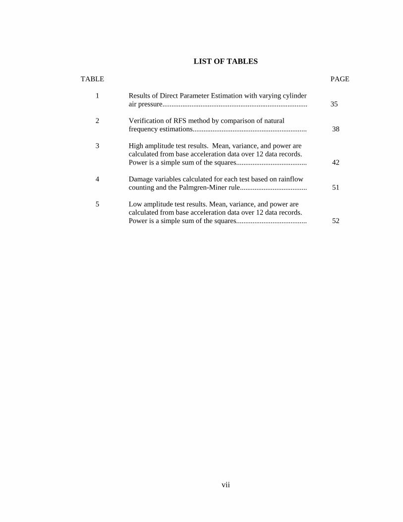
LIST OF TABLES

TABLE PAGE

1 Results of Direct Parameter Estimation with varying cylinder air pressure................................................................................

35

2

Verification of RFS method by comparison of natural frequency estimations...............................................................

38 3

High amplitude test results. Mean, variance, and power are calculated from base acceleration data over 12 data records. Power is a simple sum of the squares.......................................

42 4

Damage variables calculated for each test based on rainflow counting and the Palmgren-Miner rule.....................................

51 5

Low amplitude test results. Mean, variance, and power are calculated from base acceleration data over 12 data records. Power is a simple sum of the squares.......................................

52

viii

LIST OF FIGURES

FIGURE PAGE

1 Schematic of the apparatus. 1. Shaker; 2. Granite base; 3. Slip table; 4.Linear bearing; 5. Back mass; 6. Specimen supports; 7. Pneumatic cylinder supports; 8. Rails; 9. Front cylinder; 10. Front mass; 11. The specimen; 12. Bearing blocks; 13. Back cylinder; 14. Flexible connector……………

10

2

Model views of the apparatus. Top left: Granite base. Top right: Slip table mounted to linear bearings. Bottom Left: Zero axial backlash flexible coupling. Bottom Right: System components mounted to the slip table..........................

10

3

Solid model of the specimen. The machined notch can be seen in the center, the round hole on the left and the oblong slot on the right.........................................................................

12 4

Solid model of the original support design (Left) and the modified support (Right)...........................................................

13

5

Photograph of the ball bearing set screw shown mounted in the support tower. Before testing begins the screw is tightened against the face of the specimen and the nut is tightened to resist loosening due to vibration...........................

14

6

Photograph of the completed system........................................

15

7

Solid model showing all electrical connections to the specimen. The polarity must be kept as shown. Also note the staggered positioning of the ACPD lead wires (top)..........

16

8

Frequency response function with varying excitation amplitudes................................................................................

28

9

Simplified mass-spring-damper model of the fatigue testing apparatus...................................................................................

29

10

The distribution of data points within the phase plane (left). The data used to generate the Restoring Force Surface (right) is outlined by the dark dashed box............................................

30

11

Slice view of the RFS at �̇� = 𝟎 (top) and 𝒙 = 𝟎 (bottom)……

31

12

The RFS based on the nonlinear system model (left) and the error between the modeled surface and the calculated RFS (right).........................................................................................

33

ix

FIGURE PAGE

13

Relationship between nonlinearity and vibration amplitude.....

36

14

Weighting function based on the distribution of data used to perform weighted least squares for DPE, accentuating areas with a large amount of data.......................................................

37

15

Comparison of the original chaotic and surrogate data signals (left and righ columns respectively). Histogram of the time series data (top row) periodogram of the time series (bottom row)...........................................................................................

41

16

Histogram of the base acceleration data of the Random and Chaotic signals (left and right respectively)…………………..

43

17

ACPD signal reading normalized for direct comparison to the tracking results. (Results from Chaotic test 1-B)……………..

44

18

Estimation of embedding parameters using AMI for delay (left) and dimension (right) which are 𝜏 = 7 and 𝑑 = 4 (results from test 1-B)...............................................................

45

19

The ACPD signal reading from test 1-B (red) and the tracking results of the PSW and SOD (blue). The Damage metrics have been normalized for comparison..........................

46

20

The ACPD signal reading from test 2-A (red) and the tracking results of the PSW and SOD (blue). The Damage metrics have been normalized for comparison..........................

47

21

S-N curve used for evaluation of the damage sum, 𝐷: 𝑦 = 𝑎e𝑏log10(10) with the parameters 𝑎 = 4.3 × 104 and 𝑏 = 0.26....................................................................................

49

22

Beam diagram with applied forces. Because of the inertial force the shear and moment distribution changes shape, however we are concerned with the moment (related stresses).....................................................................................

50

23

Image of machined notch and fatigue crack at 40X magnification.............................................................................

53

24

Cycle counting of five data records on tests 8-A and 8-B (red and blue respectively). A larger number of cycle counts in the low stress range are prominent in the Random test, possibly attributing to the longer TTF......................................

54

x

FIGURE PAGE

25

Smooth trends (dashed blue) projected onto the ACPD signal (solid red). Top left: first smooth trend; Top right: first two smooth trends; Bottom left: first three smooth trends; Bottom right: first four smooth trends...................................................

56

1

CHAPTER 1

INTRODUCTION

Material fatigue has been a long standing topic of interest, and the question of

“why things break” has been addressed by many researchers in multiple disciplines of

engineering. Fatigue is studied to understand how and or when a structural element

will fail. Historically, tragic incidents such as the Versailles rail accident and the

Comet aircraft crash (1842 and 1945 respectively) have compelled researchers to

study fatigue (Smith & Hillmansen, 2004). Regardless of the efforts of countless

researchers events such as the August 1, 2007 collapse of the I-35W bridge located in

Minneapolis, Minnesota remind us that fatigue failures can still prove catastrophic

today.

Advances in solid mechanics have been made and various fatigue models based

on linear damage rules and crack growth models are available (Fatemi & Yang, 1998).

The study of linear elastic fracture mechanics has provided us with the Paris Law

(Sanford, 2003), and experimental studies have given us design criteria in the form of

the Palmgren-Miner Rule (Budynas & Nisbett, 2008). Both are used and accepted

within the scientific and industrial communities. However, these methods require very

specific and difficult to obtain a priori knowledge about the component and initial

states of damage, such as crack length or micro damage distribution.

2

The Palmgren-Miner rule is a very simple form of a cumulative fatigue damage

model. It is a stress-based method which relies on the use of S-N curves. An S-N

curve simply relates fatigue life in numbers of cycles, 𝑁, to an applied stress. The

Palmgren-Miner rule assumes that damage is a cumulative sum described as 𝐷 =

∑ 𝑛𝑖/𝑁𝑖𝑖 where 𝑛𝑖 is the number of applied cycles and 𝑁𝑖 is the total number of

cycles to failure at the stress level 𝜎𝑖 (𝑁𝑖 is obtained from an S-N curve of the testing

material). In other words, this rule states that the damage accumulated at each i-th

stress level is cumulative and can be superimposed to calculate the total damage and is

independent of the loading history. Variable loading is addressed with a combination

of cycle counting, where variable load histories are broken into a number of constant

load cycles, and the Palmgren-Miner rule. An example of this practice is a study on

the fatigue life of steel girders on the Yangpu cable-stayed bridge (built in Shanghai,

China) based on variable loading due to wind buffeting (Gu, Xu, Chen, & Xiang,

1999). This theory also ignores the presence of small stress cycles which lie below the

fatigue limit, which may or may not affect the total fatigue damage.

The Paris Law is a fatigue crack propagation model which has been derived from

linear elastic fracture mechanics. A classical form of the Paris equation [Paris 1961] is

( ) ,mda C KdN

= ∆ (1.1)

where 𝛥𝐾 = 𝑌𝜎√𝜋𝑎 is a stress intensity factor, 𝑎 is crack length, 𝐶 and 𝑚 are

material constants, and 𝑌 is a geometry factor. There exists a threshold value, 𝐾𝑡ℎ ,

below which crack propagation will not occur. This can be likened to the fatigue limit

evident on a typical S-N curve. The downfall to this method is the requirement for

3

previous knowledge of initial crack length. This type of microscopic information is

very hard and often impossible to obtain in real world applications. A second issue is

the consideration of variable amplitude loading rather than cyclic amplitude loading.

Unlike the Miner rule, Paris’ equation does not discount the affects of loading history

and this becomes a much more complicated problem. Methods such as the Wheeler

model require cycle-by-cycle integration of crack growth which attempt to include the

affects of over-stressing and are both very complicated and computationally expensive

(Anderson, 1995).

There exists a need for the development of real time procedures, which will be

a significant improvement on the outlined damage models, to perform structural health

monitoring (SHM) and condition based maintenance (CBM) tasks. It is the aspiration

of this research to design and build a platform which can be used to empirically

investigate such a model which requires no a priori knowledge of microscopic crack

information, and will decide the state of fatigue damage of a system. The platform is

tailored to meet these research goals and includes several key features which will be

outlined.

Variable amplitude loading is possible with current fatigue testing apparatuses

(Sonsino, 2007) but they do not take into account the effects of inertial and damping

forces within a system. Typical fatigue testing machines can be classified by methods

of load application as spring forces or dead weights, centrifugal forces, hydraulic

forces, pneumatic forces, thermal dilation forces, or electro-magnetic forces (Galal &

Shawki, 1990). Systems made to study the effects of inertial loading are limited in

existence and availability. The new fatigue apparatus designed and built for this study

4

is based on the fatigue testing apparatus designed by Wiereigroch’s research group in

Aberdeen, Scotland (Foong, Wiercigroch, & Deans, 2003). The capabilities of this

system meet the requirements to achieve the research goals of the study. However the

design has been streamlined for more efficient use and cost reduction.

There are two key features of the apparatus which are necessary for the study to

be successful; the system does not ignore inertial forces, and any arbitrary type of

loading can be applied (e.g., chaotic, random, and periodic). The ability to examine

the interplay between system dynamics and fatigue crack growth is achieved by the

mass-damper style loading employed in the system. Here, unlike available fatigue

apparatuses, the fatiguing specimen is a crucial component of the system’s structure.

Therefore, the structural dynamics change drastically with the evolution of the fatigue

crack.

The driving forces are provided by a programmable arbitrary function generator.

Using this equipment any time series can be used for forcing input. In this study, time

series are generated using Matlab (Mathworks, Natick, MA) and then converted to

waveforms using Tektronix software (the details of this will be covered in the

Methodology section).

An additional feature of the system is the ability to apply loading at any R-ratio

which can be defined as min max/R σ σ= where minσ and maxσ are minimum and

maximum stresses respectively. Also, the system is very adaptable to adding,

removing or moving components as it is built on a slip table with evenly spaced

mounting holes. This will also allow for the possibility of changing the geometry of

5

the specimen. The versatility of the data acquisition (DAQ) and sensing system

allows various different measurements to be taken from the system which is useful for

alternate test configurations. A final key feature of the testing apparatus is the ability

to test at high frequencies. Currently tests are conducted in the 20-30 Hz range. Fast

turnaround times in the design process require high-cycle fatigue testing to be done

quickly, and this feature drastically reduces the time expenses necessary to run each

experiment.

A reliable model of the healthy structure (the testing apparatus and a specimen

with no fatigue crack) is necessary in order to investigate the dynamical interactions

between fatigue crack evolution, load history, and structural dynamics. The model

will describe the structural dynamics of the system, and serve as a baseline for further

modeling efforts. This model is constructed using a three-step nonlinear system

identification procedure. Standard modal analysis is only used to verify the employed

methodologies because of the nonlinearity of the system.

Our predictive model will rely also on the ability to extract generalized fatigue

damage coordinates (GFDC’s) from the system dynamics data. These coordinates

will describe the existing state of damage within the system and will be obtained using

the methods of phase space warping (PSW) (Chelidze & Cusumano, 2006) and

smooth orthogonal decomposition (SOD) (Chelidze & Zhou, 2008). These

methodologies are used in conjunction to extract underlying slow-time processes using

readily available fast-time measurements of a system. SOD is a multivariate,

multiscale data analysis method that considers both spatial and temporal

characteristics of the data. Particularly, SOD is used to find smooth orthogonal

6

coordinates (SOC’s) which have minimal temporal roughness and maximal spatial

variance over the feature vectors which are constructed by calculating some standard

or common short-time statistical measure.

The method of PSW takes advantage of the small distortions in the phase space

of the fast subsystem resulting from the slow parameter drift. The dynamical system

of the following form is considered:

( , ( ), ),f tφ= µ x x (1.2)

( , ),gφ ε φ= x (1.3)

( ),y h= x (1.4)

where m∈x is the fast dynamic variable (observable state) nφ ∈ is the hidden,

underlying, slow dynamic variable, the parameter vector µ is a function of φ , t is

the time, the rate constant 0 1ε< is defined as time-scale separation between the

slow drift and fast time dynamics, and y is a scalar quantity observed under the

smooth function ( )h x .

In (Chelidze, Cusumano, & Chatterjee, 2002) this concept was applied to an

electro-mechanical system where a cantilever beam oscillated between a permanent

magnet and an electromagnet. In this study, the scalar time series y was collected

from strain gauges mounted to the beam. The electromagnet was powered by a 9-volt

battery and the slow time process, φ , represented the change in the potential field due

to the slow discharge of the battery. Using the strain gauge data alone a PSW based

7

tracking metric was shown to have a one-to-one relationship with the depletion of the

battery’s voltage.

In (Chelidze & Liu, 2005), an experimental setup with a cantilevered beam

oscillating between two permanent magnets is used. The setup is a well known

experiment described and introduced in (Moon & Holmes, 1979). The system consists

of a cantilevered beam, with a crack initiated near the cantilever, oscillating between

two permanent magnets. The physics are simple enough for a model to be created, yet

chaos can be observed within the system. Again strain gauge data is used to capture

the fast time dynamics of the beam, and a tracking matrix, which is in relationship

with the slow-time processes of the system, is extracted using PSW and SOD. The

results show that the extracted slow time variable is in good accordance with the Paris

Law as mentioned previously and represented by equation (1.1). Major additions of

the work presented in this thesis, to the aforementioned work, are that there will be an

independent measure of crack length, which can be compared to the extracted slow

process and the system itself is more adaptable to various experimental designs.

The first main research objective was to establish a platform for the investigation

of the interplay between structural dynamics and fatigue damage accumulation.

Traditional fatigue tests ignore damping and inertial forces; however in practical real

world situations fatigue accumulation is not isolated from these effects. In turn,

fatigue accumulation will affect the parameters of the system altering the structural

dynamics. Estimations of future loading patterns will be impossible without the

knowledge of the relationship with fatigue and system dynamics. Accurate fatigue life

estimations are impossible without the knowledge of all of these aspects.

8

A second goal of this research is to perform system identification of a healthy

structure. A valid and accurate model of the system dynamics at a healthy state is

necessary to begin to understand the effects of fatigue evolution. This will serve as

the basis to any proposed modeling efforts.

The fact that many structures in real world applications are not subject to constant

amplitude loadings provides the motivation to study variable load histories. It is

currently understood that load factors are nonlinearly coupled with fatigue life. The

Miner rule is inadequate in practice. It is the intention of this study to compare

variable load fatigue life predictions with actual fatigue testing of specimens under

variable loading conditions. Furthermore, chaotic loading is compared to random

loading. Variable load history tests are conducted using a time series derived from the

Duffing’s equation and are compared to random tests which are derived using

surrogate data techniques which preserve the power spectral density and the

probability distribution function of the original chaotic time series (Schreiber &

Schmitz, 1996), emphasizing the importance of time history in fatigue models. Cycle

counting methods will be applied along with the Miner rule to investigate the

predictive effectiveness of the technique. It is hypothesized that the resulting time to

failures will not be comparable between the two types of testing. It is also

hypothesized that simple cycle count based prediction will not reflect this

phenomenon.

9

CHAPTER 2

METHODOLOGY

2.1 Mechanical System Design

The fatigue testing apparatus was carefully designed to incorporate the desirable

features and reduce the cost as compared with the Wiereigroch research group’s

fatigue apparatus. A schematic of the novel apparatus is shown in Figure 1. The

driving force of the mechanical system is a low force electromagnetic shaker (Ling

Dynamic Systems, model V722) capable of a 2.9 kN peak force and supports up to a

100 kg payload. The maximum frequency of the shaker is about 4 kHz which is well

above the design requirement. The backbone of the fatigue apparatus is a slip table

guided by four linear bearings on two parallel rails mounted to a granite base. The

granite base provides a sturdy foundation for the test setup. It is carefully aligned to

be parallel with the axis of shaker in order to reduce any unnecessary wear on the

shaker itself.

The slip table is constructed of a 25.4 mm thick aluminum plate with a 12.7 mm

aluminum breadboard mounted above. The breadboard is pre-drilled and tapped for

M6-1 bolts at regular spacing of 20 mm on center. This makes for a very adaptable

mounting surface allowing for future modifications to the specimen or the system.

The slip table is connected to and driven by the shaker. This connection is managed

by a Nexen LK-2000 linear coupling. The coupling allows for angular misalignments

10

in all directions, but has zero axial backlash and can withstand forces up to 2000 N.

This coupling, combined with the careful alignment of the slip table and granite base,

Figure 1. Schematic of the apparatus. 1. Shaker; 2. Granite base; 3. Slip table; 4.Linear bearing; 5. Back mass; 6. Specimen supports; 7. Pneumatic cylinder supports; 8. Rails; 9. Front cylinder; 10. Front mass; 11. The specimen; 12. Bearing blocks; 13. Back cylinder; 14. Flexible connector.

Figure 2 Schematic of the apparatus. 1. Shaker; 2. Granite base; 3. Slip table; 4.Linear bearing; 5. Back mass; 6. Specimen supports; 7. Pneumatic cylinder supports; 8. Rails; 9. Front cylinder; 10. Front mass; 11. The specimen; 12. Bearing blocks; 13. Back cylinder; 14. Flexible connector.

Figure 1 Model views of the apparatus. Top left: Granite base. Top right: Slip table mounted to linear bearings. Bottom Left: Zero axial backlash flexible coupling. Bottom Right: System components mounted to the slip table.

11

should provide adequate protection to the internal bearings of the shaker.

The remainder of the apparatus is then constructed on top of the slip table. Two

specimen support towers are mounted to the slip table. The specimen is a simply

supported beam free to rotate about both pins and translate about one. The specimen,

shown in close detail in Figure 3, has a round hole on one end and an oblong slot on

the opposite end. It is crucial for contact between the specimen and the support pin to

be maintained, while still meeting the simply supported condition. The support pins

are made of steel tightly held to a tolerance of 12.7 mm. The hole of the specimen is

machined to 12.700 mm and reamed to 12.725 mm providing a very tight fit between

the pin and specimen. This is not a practical approach to maintain contact on the slot

side of the specimen, and this issue will be addressed in a later portion of the design

description.

The fatigue-inducing stresses are generated from the inertial masses

(approximately 5.8 kg each). Each mass is mounted to a bearing block guided by

linear rails. Two pneumatic cylinders are employed to keep the masses in constant

contact with the specimen. The pneumatic cylinders are connected to a constant air

supply and the pressure inside each cylinder is fully controllable by an air pressure

regulator. Therefore, the stresses in the specimen can be altered by simply changing

the pressure within the cylinders.

One obstacle in the design was the method of securing the beam in the vertical

direction along the pin. In order to keep the condition of a simply supported beam, the

ends of the specimen have to be free of clamping, but need to have a force keeping

12

them from lifting. Initially the beam was held between two brass bushings which were

in direct contact with the beam. This type of constraint required the tolerance on the

specimen to be very tight in order to avoid modifications to the clamping structure.

Audible clicking, indicative of under-clamping, coming from the specimen support

area were observed on multiple occasions during initial testing. Also, over-clamping

was evident in multiple tests. This was characterized by unusually long failure times

and very long crack lengths. The solution to this problem was to modify the existing

support system. Minimal changes were desired to avoid costly and time consuming

re-machining. A simple, yet effective solution, shown in Figure 3, was to incorporate

a spring in the design of the specimen support. A relatively stiff die spring was

selected with a spring constant of 140 kN/m. The tolerance of the specimen material

is ±0.203 mm. Therefore, with no adjustment the maximum change in force is only

±28.5 N. The spring is mounted along the support pin and between the specimen and

Figure 3. Solid model of the specimen. The machined notch can be seen in the center, the round hole on the left and the oblong slot on the right.

13

the top bushing. A brass washer is included between the specimen and the spring in

order to act as a bearing and maximize the contact area for an evenly applied spring

force. The only components which needed to be machined were the two risers. Their

proper height was determined by assembling the new setup without the risers, relying

on the bolts and the spring force to keep the assembly together. The bolts were

adjusted, increasing the compression on the spring, while the setup was also tested for

freedom of rotation of the specimen about the pin. Once a proper height was

established, the distance for the riser was measured. It should be noted that this new

support structure was adapted on both support towers.

Another tolerance issue is the joint between the slot and the pin. It is manageable

to hold a tight tolerance on a round hole, however the slot width varies slightly from

specimen to specimen. If the slot is too tight it will not receive the pin and if the slot

is too wide the play will cause constant collisions between the specimen and the pin.

In order to eliminate this play while maintaining the condition that the beam is free to

rotate and translate about the pin, a ball bearing set screw was added to the design.

Figure 4. Solid model of the original support design (Left) and the modified support (Right).

14

The screw is a normal set screw with a steel roller ball mounted at its tip. A tapped

hole was made at the correct height, in order for the center of the ball to contact the

center of the specimen, through the slot side support base. This can be seen in the

photograph provided (Figure 4). Before each experiment begins, the specimen is

mounted and the set screw is tightened to make contact. Because the steel ball bearing

is much harder than the aluminum the support tower can be unbolted and slid along

the slot. This forms a shallow groove in the specimen in which the ball bearing is

seated, with no play. The force from the screw keeps the specimen in constant contact

with the pin while conserving all simply supported beam conditions.

2.2 Specimen Design and Preparation

The specimen is made of aluminum 6061-T6 bar stock with initial dimensions of

1828.80 mm × 25.40 mm × 6.35 mm (l × w × t). The final dimensions of each

machined specimen are 314.71 mm × 20.32 mm × 6.35 mm. A drawing for the

Figure 5. Photograph of the ball bearing set screw shown mounted in the support tower. Before testing begins the screw is tightened against the face of the specimen and the nut is tightened to resist loosening due to vibration.

15

specimen can be found in APPENDIX A. To initiate fatigue more easily and increase

stress concentration in the beam, a V-notch is machined in the center of the specimen.

The notch is cut to a depth of 7.62 mm by a blade 0.762 mm thick with a 60 degree V-

shaped tip.

Since aluminum 6061 is heat treatable, the specimens are all fully annealed

(reduced from T6 to T0) to remove stress from the manufacturing or machining

processes, in order to keep the specimens as consistent as possible. The procedure for

heat treating is relatively simple. The specimens are loaded into a heat treating oven,

which is pre-heated to 775o F and left to sit for a minimum of two hours. After which

point the oven is shut off and the specimens are allowed to slowly cool. The rate of

cooling must be lower than 50o F per hour. This is easily achieved by the insulative

properties of the oven.

Figure 6. Photograph of the completed system.

16

The hole and slot must be machined after annealing to avoid the issue of thermal

expansion of the holes. Reaming a round hole is not a difficult task, but the slot is

very difficult to open up if these are machined prior to annealing. The machining is

done relatively far away from the crack tip and surrounding area so it is assumed there

are no major stresses induced from this process.

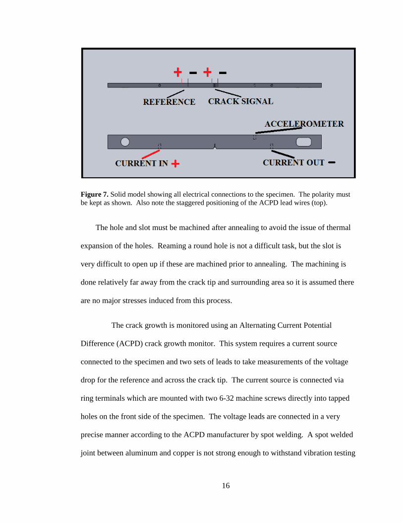
The crack growth is monitored using an Alternating Current Potential

Difference (ACPD) crack growth monitor. This system requires a current source

connected to the specimen and two sets of leads to take measurements of the voltage

drop for the reference and across the crack tip. The current source is connected via

ring terminals which are mounted with two 6-32 machine screws directly into tapped

holes on the front side of the specimen. The voltage leads are connected in a very

precise manner according to the ACPD manufacturer by spot welding. A spot welded

joint between aluminum and copper is not strong enough to withstand vibration testing

Figure 7. Solid model showing all electrical connections to the specimen. The polarity must be kept as shown. Also note the staggered positioning of the ACPD lead wires (top).

17

so the joint is reinforced using a two part epoxy which is specially formulated for high

vibration situations. The connection between the lead and ACPD monitor is made

using snap plug terminals which are isolated using electro-magnetic interference

(EMI) shielding. An accelerometer is also mounted directly to the beam which simply

requires one 5-40 tapped hole. The locations and orientations of all of these mounts

can be seen in Figure 6.

When using the eddy current sensor to measure the displacement of the beam, it is

necessary to mount, using double sided tape, a small aluminum plate to the specimen.

It is required because the beam itself is too thin for the eddy current sensor to work

properly. The dimensions of this plate are 25.400 mm × 12.700 mm × 3.175 mm.

2.3 Sensing/DAQ system

The system is monitored by a variety of sensors during each test and test set up

including an eddy current sensor, piezoelectric accelerometers, pressure transducers,

and load cells. Two single-axis accelerometers from PCB Piezoelectronics, model

number 333B42, are used. A sensitive axis of each accelerometer is always kept

parallel with the horizontal x-axis. These accelerometers are used to measure the

dynamics of the system. Typical experimental configuration will use one

accelerometer mounted to the rigid slip table and the other mounted to one of the two

inertial masses. A third accelerometer also from PCB Piezoelectronics, model number

352C66, is mounted directly to the specimen via a tapped 5-40 hole. An eddy current

displacement sensor from Lion Precision, model number U5 with driver number

ECL202, is used to measure the displacement of one of the masses or the beam

directly. These configurations will vary depending on the type of test being

18

conducted. Two PCB load cells are mounted in line between each mass and its

associated pneumatic cylinder. These can be used to track the restoring force in the

system. Two pressure transducers from PCB Piezoelectronics, model number

208C02, are mounted to the pneumatic cylinders. These are used during experimental

setup to ensure accurate pressure levels in each cylinder. All data from the sensors are

recorded at 1 kHz using a DAQ card from National Instruments connected to a PC and

all control and DAQ tasks are implemented through a LabView program.

The drive signals for the shaker are generated by a Tektronix arbitrary function

generator, model AFG 30222, which can produce standard output signals such as

Gaussian noise and sinusoid. It also has the ability to output an arbitrary waveform

which is programmed from any time series. The output signal is run through a low

pass filter with cutoff frequency, set depending on the type of signal, in order to

protect the system from high frequency components. The amplitude and frequency of

the output signal can be controlled via a USB interface and the LabView environment.

The signal is turned on and off (by a simple relay switch which uses the analog output

capabilities of the DAQ card) when the system is ready to run and when the failure

criteria has been met respectively. During a fatigue test the criteria for failure is

reached when the specimen deforms to the point beyond the saturation of the eddy

current sensor which measures the displacement of the beam. This feature is

particularly useful for long time tests as no operator is required to monitor the system.

2.3 Testing Procedure

The experimental procedure is the same for all types of test run with only varying

sensor locations or configurations of loading. The first step of any test is to prepare

19

the specimen. The voltage leads for the ACPD should be spot welded and epoxied

prior to experimentation. At this point the current cables can be attached. It is very

important to mount the cables with the correct polarity Figure 6. The positive current

cable is mounted to the hole-side of the specimen and the negative cable is mounted to

the slot side. This should be consistent with the polarity of the lead wires of the

reference and signal measurements. The positive cable runs across the front edge of

the specimen on the bottom face and is then secured using common tape in order to

reduce signal variation due to movement of the cable. Both the current cables and

voltage leads should be twisted around each other to reduce electromagnetic

interference (EMI). Once the cables are mounted, and if the eddy current sensor is

used to measure the displacement of the beam, the aluminum plate can be attached to

the specimen in the proper location. The accelerometer must be screwed into its

receiving hole and tightened securely. The beam can then be slid onto the pins, and

the electrical connections to the sensing system can be made; the leads are connected

using snap plug terminals and the current cables are connected using spade terminals.

All coincident surfaces between specimen and structure must be greased in order

to reduce friction forces. Once the grease is applied, the ball bearing ball screw can be

tightened up to the specimen and its lock nut can be tightened. The washer and spring

can be stacked and the risers and support cap can be secured. The hole-side does not

need to be checked as the free rotation condition is very easy to maintain. However,

for each test the support tower on the slot-side must be disconnected from the slip

table and forced along the lateral direction until it is free to translate along the slot.

The support tower can then be reconnected to the slip table.

20

Once the specimen is in place and fully clamped, the masses can be moved to

touch the specimen and the pneumatic cylinders can be pressurized. It is important to

adjust the pressure in both cylinders equally as not to bend or deform the specimen in

any manner. This can be done by simply turning both valves slowly at the same time.

The pressure is measured in each cylinder by the pressure transducers and their output

is displayed on an oscilloscope. The regulator is tweaked until the desired pressure

(which can vary depending on the test) is reached. The eddy current sensor can then

be positioned. If the experiment is a fatigue test, then the sensor mount is pressed set

against the sensor plate with a shim of thickness 0.584 mm and the mount can then be

tightened. Because the condition for failure is met when the beam deforms to a certain

distance from the sensor it is very important to keep the initial distance between the

sensor and the specimen as consistent as possible for all fatigue tests. Otherwise, if

the eddy current sensor is to measure the displacement of one of the masses for a

system identification test, the sensor can be located close to the mass plate; the output

from the sensor should be around 4-5 V.

The setup is now complete and the shaker can be connected to the output signal.

It is very important to never connect the shaker to a live output signal. Also, the gain

of the signal must always be slowly ramped up to avoid sudden input jumps which can

damage the shaker. The PC LabView program can be started and data collection will

begin. An Excel report will automatically be generated and the operator can fill in

pertinent information.

21

2.4 Modal Analysis

Modal Analysis is used during the system identification process. The test setup is

quite different from the previously defined system. The modal analysis is used during

the system identification procedure to detect nonlinearity in the system. An ACE data

acquisition card and Signal Calc modal analysis software from Data Physics is used.

The frequency response function (FRF) is calculated from data averaged over 16

windows of burst-random excitation. This excitation was chosen to mitigate spectral

leakage. Eighty percent of the window size is dedicated to random excitation, while

the remaining twenty percent is zero-level excitation. In the experiments, the input

signal was from an accelerometer mounted to a rigid support, while the output signal

was from an accelerometer mounted to the front mass. Both signals are high pass

filtered at 5Hz in order to remove low frequency uncertainties related to

accelerometers.

2.5 Algorithm: PSW and SOD

Recorded scalar fast-time accelerometer data, 1{ ( )}Mny n = , is collected over

consecutive data records of length D st Mt= , where st is the sampling frequency (1

kHz in this case) of the DAQ system and 𝑀 is the number of points in each data

record. The size of each data record is large enough to adequately describe the fast-

time dynamics of the system. The fast-time phase space of the scalar time series

{𝑦(𝑛)} is then reconstructed using delay coordinate embedding where

T[ ( ), ( ),..., ( ( 1) )] dn y n y n y n dτ τ= + + − ∈y , where τ is the time delay based on

average mutual information, d is the embedding dimension based on the method of

22

false nearest neighbors and T is used to denote transpose. The embedding parameters

are determined using techniques discussed in (Kantz, Holger, & Schreiber, 2004).

A metric which is in one-to-one smooth relationship with damage variables in the

reconstructed fast-time phase space is needed. That metric is first introduced in

(Chelidze, Cusumano, & Chatterjee, 2002) and is further extended in a

multidimensional form in (Chelidze & Cusumano, 2004). The metric provides a

measure of deformation of the fast-time phase space trajectories due to slow time

parameter drift. A detailed discussion is provided in (Chelidze & Cusumano, 2006),

advocating the advantages of the short-time statistic over conventional long-time

statistics. The metric is called the phase space warping function (PSWF) and is

defined as

1( ; ) ( ; )R n n n Re φ φ+ −y y P y , (2.1)

where ny is a point in the reconstructed phase space for the current damage state φ ;

1n+y is its image one time step later; and 𝑷(𝒚𝑛;𝜙𝑅) ≜ 𝑦𝑛+1𝑅 is the image of 𝒚𝑛 for a

reference or healthy damage state 𝜙𝑅.

In (Chelidze & Cusumano, 2004), for developing a multi dimensional tracking

vector, it was proposed to partition the phase space into small disjoint hyper cuboids

(𝐵𝑖, 𝑖 = 1, … ,𝑁𝑑) and evaluate the expected value of the PSWF in each region,

𝑒𝑖(𝜙) = 1𝑁𝑖∑ ê𝑦∈𝐵𝑖 (𝜙;𝒚), (2.2)

23

where 𝑁𝑖 is the number of points in 𝐵𝑖 and ê is an estimate of the PSWF, using some

data-based model for 𝑷(𝒚,𝜙𝑅). All these averaged PSWF’s are assembled into an

𝑚 = 𝑑𝑁𝑑-dimensional feature vector for each observation {𝑗}𝑗=1𝑞 ,

𝒆𝑗 = �𝑒1(𝜙); 𝑒2(𝜙); … ; 𝑒𝑁𝑑(𝜙)�, (2.3)

where semicolons indicate column-wise concatenation.

It was demonstrated in (Chelidze & Cusumano, 2004) that these feature vectors

can be projected onto actual damage states if the total change in the damage state is

small. The feature vectors were stacked in a time sequence as row vectors into a

tracking matrix 𝒀 ∈ ℝ𝒒 × 𝒎. It was then observed that SOD of this tracking matrix

provided the reconstructed damage phase space that was in direct relationship with the

actual phase space.

SOD is performed using general singular value decomposition of the matrix 𝒀

and its time derivative 𝑫𝒀, where 𝑫 is a discrete differential operator:

𝒀 = 𝑼𝑪𝑿T and 𝑫𝒀 = 𝑽𝑺𝑿T, (2.4)

where 𝑼 and 𝑽 are unitary matrices; 𝑪 and 𝑺 are diagonal matrices; and 𝑿 is a square

matrix. The smooth orthogonal coordinates (SOCs) are given by the columns of

𝜱 = 𝑼𝑪, smooth orthogonal modes (SOMs) are provided by the columns of 𝜳 = 𝑿−T

and smooth orthogonal values (SOVs) are 𝜎 = diag(𝑪𝑇𝑪) diag(𝑺T𝑺)⁄ . The dominant

SOVs hold information about the dimensionality of damage phase space and the

corresponding SOCs reconstruct that phase space. In (Chelidze 2005) and (Chelidze

24

2006) this algorithm was successfully applied to the tracking and prediction of fatigue

damage evolution.

2.6 Surrogate Data

A surrogate time series is generated using an algorithm designed to preserve

certain statistics and characteristics of the original time series. The algorithm used in

this study is introduced in (Schreiber & Schmitz, 1996). The purpose of using

surrogate data is typically for the detection of nonlinearity (Kantz, Holger, &

Schreiber, 2004). The algorithm has been adopted for this research in order to

compare damage due to chaotic and random loading. It is necessary to study two

signals with the same probability distribution (accordingly mean and variance and all

other related statistics will be preserved) and power spectrum density (PSD). The time

history, however, will be randomized.

It is very easy to randomize the time history and almost as easy to preserve the

PSD. However, an iterative process is required to meet the desired conditions.

Throughout this process the subscript 𝑘 is used to denote a list of indices, 𝑛, decided

by the sorting of the magnitudes of the series in question. The first step in the

algorithm is to store a copy of the original data, {𝑥𝑛}𝑛=1𝑁 , sorted by magnitude, {𝑐𝑘} as

well as the amplitudes of the Fourier transform of the data, {|𝑆𝑛|2}𝑛=1𝑁 . To begin,

there is a random shuffle of the data to give {𝑟𝑛0}𝑛=1𝑁 , where the superscript indicates

the iteration. The iteration is as follows:

25

1) The Fourier transform of �𝑟𝑛𝑖�𝑛=1𝑁

is taken, the amplitudes are replaced

with {|𝑆𝑛|2} and the inverse Fourier transform is performed leaving

{𝑧𝑛𝑖 }.

2) The first iteration will be repeated after transforming �𝑧𝑛𝑖 � → {𝑟𝑛𝑖+1}

by replacing the sorted magnitudes {𝑧𝑘𝑖 } with {𝑐𝑘} to get {𝑟𝑘𝑖} and re-

ordering �𝑟𝑘𝑖� → {𝑟𝑛𝑖+1}.

The surrogate will have exactly the same probability distribution, with a very close

PSD. As the number of iterations increases the error between the PSDs of the original

and surrogate series will converge to some minimal error.

2.7 Cycle Counting

A very simple rainflow counting algorithm is implemented. The main objective

of rainflow counting is to break a variable load history signal into an equivalent

sequence of constant amplitude cycles. Once cycle counting is performed the linear

Palmgren-Miner damage law can be applied for fatigue life predictions. The

algorithm outlined here is described in (Downing & Socie, 1982).

The algorithm is intended for analyzing data after collection has been completed,

and not real time computations. Two rules, which define the range of each peak and

valley, must be kept in mind throughout the algorithm:

𝑋 = range under consideration

𝑌 = previous range adjacent to 𝑋

Each peak or valley is put in a vector 𝑬(𝑛) as it is encountered.

26

The history must first be rearranged to begin and end with the maximum peak (or

minimum valley). Four simple states are then used to count the cycles; they are as

follows:

1) Read the next peak or valley; stop if out of data.

2) Form ranges X and Y; if the vector contains less than three points go to 1.

3) Compare ranges X and Y

a. If 𝑋 < 𝑌, go to 1.

b. If 𝑋 ≥ 𝑌, go to 4

4) Count range Y; discard the peak and valley of Y; go to step 2.

The algorithm then gives the equivalent cycles once all peaks and valleys have been

discarded and no data remains.

27

CHAPTER 3

SYSTEM IDENTIFICATION

In this chapter a system identification (SID) approach is implemented in order to

characterize and better understand the new system. The goal is to develop a reliable

model of the healthy structure. A three step process (which includes detection of

nonlinearity, model selection, and parameter estimation) is adopted. Also additional

discussions about nonlinearity will be provided.

3.1 Detection of Nonlinearity

The ability to detect nonlinearity has potential applications in structural health

monitoring. Related approaches are reviewed in [Farrar 2007]. The frequency

response function (FRF) overlay approach was used in this case. The concept of this

approach is that the FRF of a linear system is independent of excitation amplitude.

This, however, is not true for a nonlinear system. Therefore, nonlinearity can be

detected by changes in the FRF associated with changes in excitation amplitude.

Standard modal analysis is conducted as described in section 2.4. Three tests

were conducted at amplitude levels small, medium and large. The corresponding

FRF's are shown in Figure 7. With the increase of excitation amplitude the peak of the

FRF clearly shifts towards the lower frequency range. This is indicative of a softening

spring behavior.

28

3.2 Nonlinear Model Selection

The major challenge of nonlinear system identification is model selection (Hong,

Mitchell, Chen, Harris, Li, & Irwin, 2008). Because the system is not very

complicated, a two step procedure is adopted to determine a system model. The first

step is to build a simple physical model with some unknown functions. The method of

the Restoring Force Surface (RFS) will then be used as the second step to determine

the unknown functions.

The assumptions that the slip table and fixtures are rigid, and the deformation of

the specimen is relatively small (< 2 × 10−4 m from its equilibrium position), allows

the testing rig to be represented by a single degree of freedom mass-spring-damper

system shown in Figure 8.

The specimen is modeled as a linear spring (with stiffness 𝑘𝑠). The pneumatic

cylinders are represented by a combination of nonlinear springs (𝑘1 and 𝑘2) and

Figure 8. Frequency response function with varying excitation amplitudes.

29

nonlinear dampers (𝑐1 and 𝑐2). The system can be described by the differential

equation in the form of:

𝑚�̈� + 𝑐1(𝑥, �̇�) + 𝑐2(𝑥, �̇�) + 𝑘1(𝑥, �̇�) + 𝑘2(𝑥, �̇�) + 𝑘𝑠𝑥 = 𝑚𝑎 (3.1)

where, 𝑚 is the addition of the two masses; 𝑎 is the base acceleration; 𝑥 is the relative

displacement measured by the eddy current sensor, and dots represent time

differentiation. Further simplification can be made resulting in:

𝑚�̈� + 𝐶(𝑥, �̇�) + 𝐾(𝑥, �̇�) + 𝑘𝑠𝑥 = 𝑚𝑎 (3.2)

where 𝐶(𝑥, �̇�) = 𝑐1(𝑥, �̇�) + 𝑐2(𝑥, �̇�) and 𝐾(𝑥, �̇�) = 𝑘1(𝑥, �̇�) + 𝑘2(𝑥, �̇�).

Restoring force is defined as a variable force that gives rise to equilibrium in a

physical system and can be written as:

𝑓(𝑥, �̇�) = 𝐹 −𝑚�̈� (3.3)

Figure 9. Simplified mass-spring-damper model of the fatigue testing apparatus.

30

for a SDOF system, where 𝐹 is the external force and 𝑚 is the mass. In our case, the

restoring force equals:

𝑓(𝑥, �̇�) = −𝑚𝑎 −𝑚�̈� = 𝐶(𝑥, �̇�) + 𝐾(𝑥, �̇�) + 𝑘𝑠𝑥 (3.4)

The related restoring force surface (RFS) approach is one of the most well

established nonlinear system identification methods available. Although we do not

plan to apply the RFS method directly, the RFS can provide valuable information for

model selection. Among all the parameters, mass is measured directly, 𝑎 is measured

by an accelerometer, 𝑥 can be measured by the eddy current sensor, and �̇� and �̈� can

be estimated using the finite difference method. Therefore, the RFS can be directly

generated based on collected data sets.

The restoring forces are calculated using 6 × 105 data points, while the testing rig

is driven by a random signal with limited frequency band (0 to 60Hz). The amplitude

of the excitation was chosen to ensure the availability of parameter identification data

within the range of proposed experimental excitation amplitudes. The pressure in the

Figure 10. The distribution of data points within the phase plane (left). The data used to generate the Restoring Force Surface (right) is outlined by the dark dashed box.

31

two pneumatic cylinders is set to 103 kPa. The data is recorded at a DAQ frequency of

1 kHz and the distribution of sample points on the phase plane are shown in Figure 9.

Isolated points related with discrete measurements are interpolated into a

continuous surface using Sibson's natural neighbor method (Sibson, 1985), and the

measured RFS is shown in Figure 9.

Two slice views of the RFS are shown in Figure 10 with 𝑥 = 0 and �̇� = 0

respectively. It is a reasonable assumption that 𝐶(𝑥, �̇�) is a function of �̇� only and

𝐾(𝑥, �̇�) is a function of 𝑥 only; 𝑓 = 𝐶(�̇�) when 𝑥 = 0 and 𝑓 = 𝐾(𝑥) + 𝑘𝑠𝑥 based

on this assumption. From Figure 10, we can conclude that 𝐶(�̇�) and the 𝐾(𝑥) can be

described partially by cubic polynomials. However, it is also suspect that Coulomb

damping is present in the system. A good experimental fit of the restoring force with

Coulomb damping (Olsson, Astrom, Canudas de Wit, Gafvert, & Lischinsky, 1998)

can be described as

Figure 11. Slice view of the RFS at �̇� = 𝟎 (top) and 𝒙 = 𝟎 (bottom)

32

𝐹 = 𝐶|�̇�|𝛿𝑣sgn(�̇�) (3.5)

where 𝐹 is the restoring force and 𝛿𝑣 is a scaling parameter dependent on geometry.

Therefore, equation 3.2 can be rewritten in the form:

𝑚�̈� + 𝐶𝑓1�̇� + 𝐶𝑓2�̇�3 + 𝐶𝑓3|�̇�|𝛼sgn(�̇�) + 𝐾𝑓1𝑥 + 𝐾𝑓2𝑥3 + 𝐾𝑓3|𝑥|𝛽sgn(𝑥)

= 𝑚𝑎

(3.6)

where 𝐶(�̇�) = 𝐶𝑓1�̇� + 𝐶𝑓2�̇�3 + 𝐶𝑓3|�̇�|𝛼sgn(�̇�) and, 𝐾(𝑥) = 𝐾𝑓1𝑥 + 𝐾𝑓2𝑥3 +

𝐾𝑓3|𝑥|𝛽sgn(𝑥).

3.3 Parameter Estimation

With a nonlinear model, the system parameter estimation problem can be solved.

The method of direct parameter estimation (DPE) (Mohammad, Worden, &

Tomlinson, 1992) will be used. To perform DPE, Eq. 3.6 is rewritten for 𝑛 discrete

measurements in the form of Eq. 3.7. However, because of the exponents, 𝛼 and 𝛽, the

error must be reduced iteratively. DPE is performed while varying 𝛼 and 𝛽 over a

predetermined range in order to minimize the mean square error.

⎣⎢⎢⎡�̇�1 �̇�13 |�̇�1|𝛼sgn(�̇�1) 𝑥1 𝑥13 |𝑥1|𝛽sgn(𝑥1)�̇�2 �̇�𝑛3 |�̇�2|𝛼sgn(�̇�2) 𝑥2 𝑥23 |𝑥2|𝛽sgn(𝑥2)⋮ ⋮ ⋮ ⋮ ⋮ ⋮�̇�𝑛 �̇�𝑛3 |�̇�𝑛|𝛼sgn(�̇�𝑛) 𝑥𝑛 𝑥𝑛3 |𝑥𝑛|𝛽sgn(𝑥𝑛)⎦

⎥⎥⎤

⎣⎢⎢⎢⎢⎢⎡𝐶𝑓1𝐶𝑓2𝐶𝑓3𝐶𝑓4𝐶𝑓5𝐶𝑓6⎦

⎥⎥⎥⎥⎥⎤

= �

�̈�1 𝑎1�̈�2 𝑎2⋮ ⋮�̈�𝑛 𝑎𝑛

� � 𝑚−𝑚�

(3.7)

33

When 𝑛 > 6 this is an over defined problem which can be solved by using a

standard least squares approach. The parameters are determined using the data shown

in Figure 9. An RFS can then be generated based on the identified nonlinear model.

The resulting surface and the error, between the modeled surface and the RFS, are

shown in Figure 11. The results are reasonable and the error is quite low (< 16𝑁 or

10 %).

Although the two RFS's (based on the measured data and based on the model) fit

each other quite well, relatively large errors are observed in the areas when the

absolute value of 𝑥 and �̇� are large and (𝑥 �̇�) > 0⁄ . The large errors are due to three

main reasons:

1) The number of sampling points in these areas is small, which leads to

inaccurate estimation of the RFS from experimental data.

Figure 12. The RFS based on the nonlinear system model (left) and the error between the modeled surface and the calculated RFS (right).

34

2) These areas represent rare dynamical states of the rig; large displacement,

velocity, acceleration, and jerk, which make the numerical calculation of

velocity and acceleration inaccurate.

3) With a large jerk, 𝑥, a time delay between different measurement channels

on the DAQ system is not negligible and causes additional errors in the

measurement of acceleration.

3.4 Discussion

3.4.1 Dynamic Range

The system has the capacity to generate 1.6 g's of acceleration at 30 Hz. The

maximum load capacity is determined by the mass of the inertial blocks and the

maximum acceleration of the slip table. Theoretically, there is no limitation to the

frequency range of the load if the slip table and all fixtures can be treated as rigid

bodies. However, the highest frequency of applied load in real tests is limited to 30 Hz

because the natural frequency of the slip table is about 150 Hz. Further improvement

of the structural stiffness is not pursued, because higher stiffness means additional

mass for the slip table; and as a result, the maximum load capacity will decrease due to

the limitation of the shaker output power.

3.4.2 Influence of Air Pressure

The same system identification procedure is repeated several times under

different pressures (the pressure in the two cylinders is kept identical). The estimated

parameters are listed in Table 1. The relationship between the pressure and the system

35

parameters can be described as follows: the stiffness and the damping of the testing

system increase when pressure is increased.

Table 1. Results of Direct Parameter Estimation with varying cylinder air pressure.

Press (kPa)

𝐶𝑓1 �𝑁𝑠𝑚� 𝐶𝑓2 ��

𝑁𝑠𝑚�3

� 𝐶𝑓3 ��𝑁𝑠𝑚�𝛼

� 𝐾𝑓1 �𝑁𝑚� 𝐾𝑓2 �

𝑁𝑚3� 𝐾𝑓3 �

𝑁𝑚𝛽� 𝛼 𝛽

138 400.58 −6.48× 104 342.04 1.41

× 106 8.72× 1012

−8.96× 108 0.63 1.81

172 −4.18× 103

1.87× 104

3.19× 103

2.31× 106

4.56× 1013

−7.80× 109 0.82 1.93

207 −2.36× 103

−6.96× 104

2.06× 103

2.25× 106

3.99× 1013

−1.56× 1010 0.79 2.02

3.4.3 Linear Region

The system has been characterized to have nonlinear stiffness and damping.

Coulomb damping is strong at a small velocity and displacement level. However,

when the system is observed over a relatively narrow range of displacement and

velocity the system appears to be approximately linear. The definition of a linear

region is also interesting theoretically since 1) there is an advantage in system analysis

if a linear assumption holds, and 2) a change of the linear region boundary itself can

serve as an indicator for abnormality.

Here non-linearity is defined by how accurately a linear model can fit the

measured RFS. For a region 𝑅𝐺 in the phase space defined by |𝑥| < 𝑥1 and �̇� < 𝑥2, a

linear model is estimated based on Eq. 3.7 by assuming that only 𝐶𝑓1 and 𝐾𝑓1 are

nonzero. The nonlinearity (𝑁) is quantified by

𝑁 =max |𝑓(𝑥, �̇�)𝑙 − 𝑓(𝑥, �̇�)𝑚|

max |𝑓(𝑥, �̇�)𝑚|

(3.8)

36

where [𝑥, �̇�] ∈ 𝑅𝐺, 𝑓(𝑥, �̇�)𝑙 is the restoring force calculated based on the linear model,

and 𝑓(𝑥, �̇�)𝑚 is the measured restoring force.

Based on the above definition, the nonlinearity of different regions on the

response phase space is shown in Figure 12. For each pixel on the image, its

coordinates (𝑎𝑥 and 𝑎𝑦) define the region on the response phase space |𝑥| < 𝑎𝑥 and

|�̇�| < 𝑎𝑦 and its color illustrates the severity of the nonlinearity. A color bar is

provided with the map to allow for convenient interpretation of the data.

Nonlinearities under a 20 Hz sinusoidal excitation at amplitudes of 1.2 g and 1.6 g are

outlined in black and blue circles respectively. Since a 1.2g excitation is representative

of a typical experiment (1.6g is a higher limit) and its corresponding nonlinearity is

relatively low (< 15%), we can conclude that the testing rig works in a linear region

under a typical load condition.

Figure 13. Relationship between nonlinearity and vibration amplitude.

37

3.4.4 Verification

The restoring force surface method can be verified by comparing DPE with

standard linear modal analysis approaches. As outlined previously, modal analysis can

be used because it is reasonable to treat the system as a linear system if the response

amplitude is low. Verification of the restoring force method will be completed if the

results from DPE and modal analysis fit each other well.

In order to directly compare the results of the two methods, short experiments

were run using Signal Calc modal analysis software from Data Physics. In these

experiments, the response amplitude is controlled carefully, so the linear assumption

can be held. The FRF data, collected using the same parameters outlined in Section

3.1, can be fit to the known single degree of freedom FRF in the form:

Figure 14. Weighting function based on the distribution of data used to perform weighted least squares for DPE, accentuating areas with a large amount of data.

38

|𝐺(𝑖𝜔)| =𝐶𝑠

�(1 − 𝑟2)2 + (2𝜁𝑟)2

(3.9)

where 𝐺(𝑖𝜔) is the frequency response, 𝐶𝑠 is a scaling factor, 𝜁 is the damping ratio,

and 𝑟 is 𝜔/𝜔𝑛. The parameters, 𝐶𝑠, 𝜁, and 𝜔𝑛 are approximated using an iterative

method which minimizes the least squares error. In order to emphasize the

significance of the data at areas of small velocity and displacement, a weighted least

squares approach was used for DPE. The weighting function is a 3-dimensional

surface which is representative of the distribution of data across the phase space (3-

dimensional histogram). The function is normalized giving each data point a weight

between zero and one, depending on where in the phase space it exists. The weighting

factor is

𝑊 = (𝑤1𝑤2) (3.10)

where 𝑊 is the weight function shown in Figure 13, 𝑤1is the distribution function of

𝑥 and 𝑤2 is the distribution function of �̇�. The natural frequency is then calculated

using the measured mass and the linear coefficient of stiffness, 𝐾𝑓1. The results can be

seen in Table 2.

Table 2. Verification of RFS method by comparison of natural frequency estimations.

Modal Analysis Restoring Force Pressure (kPa) 𝜔𝑛 (Hz) 𝜔𝑛 (Hz)

138 86.27 91.45

172 88.45 92.11

207 106.24 104.04

39

Chapter 4

FATIGUE EXPERIMENTS

The main purpose of the novel fatigue apparatus is to study the relationship

between fatigue crack evolution and system dynamics. The design work and system

identification prove that this system is capable of meeting the goals of the research and

will be useful for further endeavors, including the study of predictive models of

fatigue failure based on fast-time system dynamics data. This ambitious goal cannot

be met in this work. The scope of this thesis is not to compile such a model, but rather

to serve as a foundation of further modeling efforts and demonstrate the effectiveness

of the apparatus.

As mentioned in the introduction one of the research goals is to observe the

interplay between structural dynamics and fatigue damage for statistically matched

chaotic and random excitations. It was hypothesized that there will be an

incommensurate relationship between the time to failure (TTF) of the specimens under

the two signal types. In order to explore this hypothesis, fatigue experiments were

conducted at two amplitude levels (high and low with maximum base acceleration of

1.7 and 1.5 g’s respectively) and the results will be discussed in separate sections. It

was also declared that the rainflow counting method would be utilized in combination

with the Palmgren-Miner rule to investigate the appropriateness of linear damage

models. The hypothesis is that this type of damage law will not reflect the results of

the fatigue life experiments.

40

4.1 Signal Generation

A chaotic signal was generated from the equations describing the Duffing

oscillator, which can be written as a periodically forced oscillator with nonlinear

stiffness:

�̈� = −𝛿�̇� + 𝛽𝑥 − 𝛼𝑥3 + 𝛾 cos(𝜔𝑡) (4.1)

where 𝛿 is the damping constant, 𝛽 is the negative stiffness constant, 𝛼 is the

nonlinear stiffness constant, and 𝛾 is the forcing amplitude. The parameters are

chosen such that the system will be in a chaotic state. This can be shown by plotting a

bifurcation diagram of the system. In this case from the bifurcation diagram the

system is chaotic for the parameters 𝛼 = 1,𝛽 = 0.6, 𝛿 = .25, 𝛾 = .2, and 𝜔 = 1.

Once the time series is generated in Matlab a nearest neighbor search is done

to find a similar state further in time. This is necessary in order to match the start and

end point of the time series as closely as possible. The function generator used to

output the signal to the shaker can only handle a maximum of 216 data points so the

signal is looped throughout the testing. Once the ends are matched up with a

sufficiently large amount of data between them, the time series is exported as a ASCII

text file and imported into Tektronix’ ArbExpress waveform generation software.

There, the signal is exported to a USB flash drive which will be used to load the signal

onto the function generator.

Because the signal is repeated periodically, the frequency of the function

generator must be set to keep the frequency of the input excitation where it is desired

41

(approximately 20-30 Hz). This is done by collecting the output of the function

generator, set at some frequency, and processing the data to get the power spectrum.

The function generator frequency is adjusted until the main frequency components of

the power spectrum fall within the desired range. For this particular signal it was

found that the frequency must be set to 20 mHz. The surrogate data set can then be

generated from the chaotic time series by using the algorithm included in section 2.6.

4.2 High Amplitude Fatigue Tests

The excitation amplitude was decided to keep the tests concise for quick

turnaround time. It is also beneficial to have relatively short data sets to save on

digital storage and computation time during data analysis. It should be noted that all

Figure 15. Comparison of the original chaotic and surrogate data signals (left and right columns respectively). Histogram of the time series data (top row) periodogram of the time series (bottom row).

42

test names are indicative of the order run and no further inference should be made.

Also, the two signals used for driving the system are henceforth called Chaotic and

Random, and it should be implicit that these signals are varied only in amplitude. The

experimental design is very straightforward. A minimum of five successful tests will

be accepted for each excitation type. This will result in a total of ten sets of data for

analysis at the high amplitude level.

The first and most obvious piece of data that gives an indication of the fatigue

process is the TTF. A clear trend emerges in the TTF data shown in Table 3. It is

obvious that the Random excitation is much more damaging to the specimen. These

test results show that the system under Chaotic excitation outlasts the system under

Random excitation by nearly a factor of two in all accounts. This data appears to be

Test Number

Excitation Signal

Time To Failure (hrs) Mean Variance Power

1-A Random 0: 53 −0.0036 0.0754 9.05 × 104

1-B Chaotic 1: 44 −0.0030 0.0728 8.74 × 104

2-A Random 1: 07 −0.0036 0.0724 8.70 × 104

2-B Chaotic 1: 50 −0.0038 0.0725 8.70 × 104

3-A Random 0: 44 −0.0035 0.0758 9.09 × 104

3-B Chaotic 1: 46 −0.0034 0.0735 8.82 × 104

4-A Random 0: 52 −0.0036 0.0763 9.15 × 104

4-B Chaotic 1: 42 −0.0037 0.0729 8.75 × 104

5-A Random 0: 45 −0.0040 0.0735 8.82 × 104

5-B Chaotic 1: 13 −0.0039 0.0725 8.71 × 104

Table 3. High amplitude test results. Mean, variance, and power are calculated from base acceleration data over 12 data records. Power is a simple sum of the squares.

Time To Failure (hrs:min)

Mean (V)

Variance (V2) Power (V2)

43

very interesting and supportive of the hypothesis that there is a strong relationship

between fatigue accumulation and time history.

The statistics are included in Table 3 to show that the statistical qualities of both

signals match well. Any drift in these statistics, from test to test, is due to the lack of a

sophisticated shaker output controller, however, these tests have proven very

repeatable and the variations in the excitation signal seam negligible at this amplitude

level. The time histories of one data set of the Random and Chaotic experiments (1-A

and 1-B respectively) can be seen in Figure 15. The histograms show base

acceleration over one data record. The probability distributions of the output signals

match identically; however, the input to the shaker is displacement. The histograms of

the acceleration of the base are not then identical under random and chaotic excitation.

It would be a very difficult problem to build a surrogate data which would match the

transformation of input displacement to acceleration. As long as the main factors such

Figure 16. Histogram of the base acceleration data of the Random and Chaotic signals (left and right respectively.)

44

as mean, and minimum and maximum acceleration are preserved, the differences are

acceptable.

4.2.1 Damage Tracking

The real fatigue is tracked using the ACPD measurement equipment. For the

high amplitude testing {𝑆𝑛}𝑛=1𝑀 , where 𝑀 = 20,000, is the scalar data record of the

ACPD signal. The sampling frequency, 𝑡𝑓, of the DAQ system is 1 kHz; therefore the

time length of each data record, 𝑡𝑠 = 𝑀/𝑡𝑓, is 20 seconds and there are 𝑁 =

�loor(𝑇𝑇𝐹 𝑡𝑠⁄ ) (TTF is time to failure in seconds) data records in each test. This data

is processed by taking the mean of the signal over each data record and concatenating

into a vector:

𝐴𝐶𝑃𝐷𝑠𝑖𝑔 = [{𝑆𝑛� }1, {𝑆𝑛� }2, … , {𝑆𝑛� }𝑁] (4.1)

The trend can then be plotted as shown in Figure 16.

Figure 17. ACPD signal reading normalized for direct comparison to the tracking results. (Results from Chaotic test 1-B)

45

Because the input signal is deterministic, tracking of the damage for Chaotic tests

can be done by using the PSW algorithm outlined in section 2.5. As mentioned

previously the time series of the mass acceleration {𝑎𝑚}𝑛=1𝑀 , again 𝑀 = 20,000, is

used for the fast-time system dynamics data. The time series needs to be embedded

using delay reconstruction with the help of the false nearest neighbors (FNN) search

for embedding dimension, 𝑑, (Kennel, Brown, & Abarbanel, 1992) and average

mutual information (AMI) for the time delay, 𝜏 (Fraser & Swinney, 1986). Typically

the delay is chosen as the first local minimum of the AMI.

The method of FNN is a straightforward concept. There should be no

intersections within the phase space if the system is governed by deterministic

differential equations, and points in a small neighborhood should be there due to the

dynamics of the system and not insufficient embedding dimension. The FNN method

finds the percentage of FNNs in the embedded phase space for a given dimension.

Figure 18. Estimation of embedding parameters using AMI for delay (left) and dimension (right) which are 𝝉 = 𝟕 and 𝒅 = 𝟒 (results from test 1-B).

46

The embedding dimension is decided when the percentage of FNNs are sufficiently

small (for example < 3%). The estimation of both parameters using mass

acceleration data from test 1-B can be seen in Figure 17.

The PSW algorithm can then be applied. The feature vector is calculated and

SOD is applied to track the damage. The results from test 1-B are shown in Figure 18.

The damage trend has obviously been captured from the fast-time data, however in

many tests the phenomenon evident in the first portion of the tracking metric are

observed. It is unclear what causes this effect, but it can be speculated that it is due to

some type of “breaking in” of the system. It is possible that the deformation of the

beam from the equilibrium position could be the cause of the phenomenon, or perhaps

there is an effect of friction between the specimen and adjoining surfaces, or some

type of relaxation in the beam from the evolving micro crack distribution.

Figure 19. The ACPD signal reading from test 1-B (solid red) and the tracking results of the PSW and SOD (dashed blue). The Damage metrics have been normalized for comparison.

47

The PSW method will not yield the best results for tracking the fatigue during

Random testing. The reason being is that the local linear model tracking metric is not

accurate for a randomly excited system. However, because the system can be

considered fairly linear under the operating conditions, a linear stochastic auto

regressive (AR) model can be used to characterize the dynamics. This type of model

can be described as:

𝑦𝑛 = �𝑎𝑗𝑦𝑛−𝑗 + 𝜂𝑛

𝑀𝐴𝑅

𝑗=1

(4.2)

Where 𝑀𝐴𝑅 is the order of the model, 𝜂𝑛is Gaussian white noise, and 𝑎𝑗 are the model

parameters. These parameters will be calculated for each data record and compose the

feature vector used for tracking the parameter drift.

The burg method, implemented in the Matlab function arburg, is used to calculate

the parameters. The feature vector is assembled as:

Figure 20. The ACPD signal reading from test 2-A (solid red) and the tracking results of the PSW and SOD (dashed blue). The Damage metrics have been normalized for comparison.

48

𝐹 =

⎣⎢⎢⎢⎡ 𝑎1

1 𝑎21 … 𝑎1

𝑁

𝑎21 𝑎2

2 … 𝑎2𝑁

⋮ ⋮ ⋮𝑎𝑀𝐴𝑅1 𝑎𝑀𝐴𝑅

2 … 𝑎𝑀𝐴𝑅𝑁 ⎦

⎥⎥⎥⎤

(4.3)

where the feature space, 𝐹 ∈ ℝ𝑀𝐴𝑅×𝑁 and 𝑁 is the number of data records. SOD can

then be applied to track the slow time drift.

The tracked damage metric can be seen in comparison to the ACPD signal in

Figure 19. Again, it is clear that the damage has been captured within the fast-time

dynamics. Also, it is noted the same phenomenon exists in the beginning of the

tracking function. This permeates most test results and it is of interest to determine

the causes in the future.

It is also worthy of noting the differences between the fatigue evolution of the

Chaotic and Random tests. Due to the time history, there is a very short to nonexistent

time span of steady crack growth observed in the Random test data as opposed to the

Chaotic results. Fracture is initiated much quicker in the Random testing, hence the

shorter fatigue life. The exact causes of this are unknown to the author or available

literature, but it can be surmised that the two signals are essentially the same and only

unlike one another in time history. Therefore this effect can be described somehow by

the information in the time history and reinforces the hypothesis that fatigue life is

strongly dependent on time history and not merely probability distribution of stress

magnitudes.

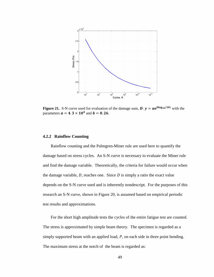
49

4.2.2 Rainflow Counting

Rainflow counting and the Palmgren-Miner rule are used here to quantify the

damage based on stress cycles. An S-N curve is necessary to evaluate the Miner rule

and find the damage variable. Theoretically, the criteria for failure would occur when

the damage variable, 𝐷, reaches one. Since 𝐷 is simply a ratio the exact value

depends on the S-N curve used and is inherently nondescript. For the purposes of this

research an S-N curve, shown in Figure 20, is assumed based on empirical periodic

test results and approximations.

For the short high amplitude tests the cycles of the entire fatigue test are counted.

The stress is approximated by simple beam theory. The specimen is regarded as a

simply supported beam with an applied load, 𝑃, on each side in three point bending.

The maximum stress at the notch of the beam is regarded as:

Figure 21. S-N curve used for evaluation of the damage sum, 𝑫: 𝒚 = 𝒂𝐞𝒃𝐥𝐨𝐠𝟏𝟎(𝟏𝟎) with the parameters 𝒂 = 𝟒.𝟑 × 𝟏𝟎𝟒 and 𝒃 = 𝟎.𝟐𝟔.

50

𝜎𝑚𝑎𝑥 = 𝑀𝑆

, 𝑆 = 𝑏ℎ2

6 (4.4)

Where 𝑆 is the section modulus, 𝑏 is the specimen thickness, and ℎ is the width, and

𝑀 = 𝑃+𝑚𝑎4 𝐿2. (4.5)

The load 𝑃 is

𝑃 = 𝑃𝑠𝑡𝑎𝑡𝑖𝑐 ≅ 𝑃𝑐𝐴 (4.6)

where 𝑃𝑐 is the pressure in the cylinder, 𝐴 is the area of the cylinder’s bore. The static

load is approximate because of the nonlinearity of the pneumatic cylinder.

The rainflow cycle counting method can then be applied to the time series of the

stress data:

Figure 22. Beam diagram with applied forces. Because of the inertial force the shear and moment distribution changes shape, however we are concerned with the moment (related stresses) at the location of the notch only. P is the static force due to the pressure within the cylinders (both cylinders have equal pressure in this testing).

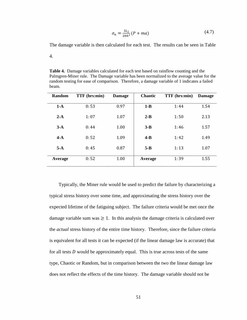
51

𝜎𝑛 = 3𝐿22𝑏ℎ2

(𝑃 + 𝑚𝑎) (4.7)

The damage variable is then calculated for each test. The results can be seen in Table

4.

Table 4. Damage variables calculated for each test based on rainflow counting and the Palmgren-Miner rule. The Damage variable has been normalized to the average value for the random testing for ease of comparison. Therefore, a damage variable of 1 indicates a failed beam.

Random TTF (hrs:min) Damage Chaotic TTF (hrs:min) Damage

1-A 0: 53 0.97 1-B 1: 44 1.54

2-A 1: 07 1.07 2-B 1: 50 2.13

3-A 0: 44 1.00 3-B 1: 46 1.57

4-A 0: 52 1.09 4-B 1: 42 1.49

5-A 0: 45 0.87 5-B 1: 13 1.07

Average 0: 52 1.00 Average 1: 39 1.55

Typically, the Miner rule would be used to predict the failure by characterizing a

typical stress history over some time, and approximating the stress history over the

expected lifetime of the fatiguing subject. The failure criteria would be met once the

damage variable sum was ≥ 1. In this analysis the damage criteria is calculated over

the actual stress history of the entire time history. Therefore, since the failure criteria

is equivalent for all tests it can be expected (if the linear damage law is accurate) that

for all tests 𝐷 would be approximately equal. This is true across tests of the same

type, Chaotic or Random, but in comparison between the two the linear damage law

does not reflect the effects of the time history. The damage variable should not be

52

related to time, and the results show a close ratio between TTF and D. This implies

again that time history is very important in fatigue accumulation.

4.3 Low Amplitude Fatigue Tests

The same signals were run at lower amplitude to investigate the fatigue

accumulation over longer test lengths. The results can be seen in the following:

Table 5. Low amplitude test results. Mean, variance, and power are calculated from base acceleration data over 12 data records. Power is a simple sum of the squares.

Test Number

Excitation Signal

Time to Failure (hrs) Mean (V) Variance (V2) Power (V2)

6-A Random 7: 25 −0.0043 0.0578 6.94 × 104

6-B Chaotic 7: 20 −0.0049 0.0593 7.12 × 104

7-A Random 7: 28 −0.0050 0.0595 7.15 × 104

7-B Chaotic 3: 49 −0.0049 0.0605 7.26 × 104

8-A Random 6: 51 −0.0040 0.0619 7.42 × 104

8-B Chaotic 21: 06 −0.0041 0.0619 7.43 × 10^4

The TTF results are not as revealing as the previous results. The Random tests

are again very consistent; however the Chaotic test results differ drastically. The

variations in the signal still exist but are not large and do not appear to have direct

relationship to the TTF. For example, the Chaotic test with the longest TTF, 8-B, has

the largest power in the signal and variance. If anything in the probability distribution

would seem to have a direct impact on TTF it would be these two statistics; however

that is not the apparent case.

53

The assumption is that the TTF relies heavily on the initial condition. This makes

sense and is rather obvious. The controllable condition is the initial cut depth of the

notch, and some uncontrollable conditions could be environmental effects, micro

crack structure, inherent material stresses, overload induced relaxations etc. The

initial crack length was examined under a Stocker and Yale optical micrometer at 40X

magnification. The crack lengths of all the fatigue tests recorded in this data were

measured to be 7.823 mm ± 0.069 mm, which is relatively consistent and likely not a

factor large enough to influence the TTF drastically. This leaves the uncontrollable

effects to be the variants in the initial condition. To investigate this further, a much

larger sample of data would need to be collected, but it would certainly be an

interesting problem to address.

Another notable feature is the fact that in this testing the Random excitation was

not always more damaging than the Chaotic. This could possibly be explained by the

Figure 23. Image of machined notch and fatigue crack at 40X magnification.

54

distribution of stress cycles. Using rainflow counting on a data sample comprised of

five data records, the stress cycles can be counted and compared. The comparison is

between tests 8-B and 8-A. The Chaotic excitation has fewer low stress cycles. This

could affect the TTF as the lower stress cycles have much less impact on fatigue

accumulation. The reason for the extended TTF of the test 8-B is likely attributed to

the initial conditions of the beam, magnified by the lower amplitude.

In general, as the amplitude decreases, the overall shape of the stress cycle

distribution would stay the same and simply shift to a lower stress range. Therefore it

is expected that the Chaotic excitation would be more damaging at a lower amplitude

on average. One test was conducted for a Random and Chaotic excitation at lower

amplitude, and this effect was produced; the Chaotic TTF was 12:55 and the Random

TTF was 31:06. Further investigation would be necessary to conclude what exactly is

Figure 24. Cycle counting of five data records on tests 8-A and 8-B (red and blue respectively). A larger number of cycle counts in the low stress range are prominent in the Random test, possibly attributing to the longer TTF.

55

happening, but the stress cycle distribution clearly has a strong relationship with the

TTF.

4.4 Discussion of Test Results

It was seen in the high amplitude fatigue tests that the Random excitation

produced very consistent time to failures, and was apparently more damaging than the

Chaotic excitation. It was also shown, by using an arbitrary S-N curve and a simple

rainflow cycle counting algorithm, that the Palmgren-Miner Damage rule was

insensitive to the time history. Both of these findings are very interesting and have

implications in the real world. From this study it is evident that the Palmgren-Miner

rule, which is widely used as an industry standard, is severely lacking in its ability to

define damage based solely on a count of stress reversals. It is evident that the order

of applied stresses is more damaging in a larger sense than purely frequency or stress

amplitudes. It is the recommendation of the author that future tests be conducted with

sinusoidal excitation of varying amplitude. This would provide the very simplest

scenario to further investigate the effects of stress time history.

Upon further testing, at a lower excitation amplitude, it is seen that the time to

failure under Chaotic excitation is much more sensitive to initial conditions of the

beam compared with the time to failure of the Random excitation tests. It was ruled

out that the only initial condition fully controllable by human interaction, the initial

length of the notch, was the factor at play. All specimens were measured and the

notch length was relatively well controlled. This leaves the initial conditions of the

specimen as the apparent major contributor to the fatigue initiation. It is also possible

56

that the Random excitation is much more effective at consistently initiating stage II

constant fatigue crack growth.

A very important problem to address is to decipher from the extracted smooth

trends which characteristics can be directly attributed to fatigue crack growth and not

some other slow process. It is evident by examining the dominant smooth trend, that

the fatigue is tracked well close to the end of the experiment. This makes sense,

because fatigue will dominate the system at this point in the experiment. However, as

pointed out previously, there is often an anomaly present in the beginning of the trend.

It will be very interesting to determine whether this anomaly is due to something such

as deformation of the beam from the equilibrium position, or fatigue directly. It is also

Figure 25. Smooth trends (dashed blue) projected onto the ACPD signal (solid red). Top left: first smooth trend; Top right: first two smooth trends; Bottom left: first three smooth trends; Bottom right: first four smooth trends.

57

possible that the fatigue can be better tracked by looking at projections of more than

one of the smooth trends. For example, by projecting the two smoothest trends onto

the ACPD signal in the least squares sense, the resulting trend follows the fatigue in

much better correspondence, especially in the constant crack growth region. This

result is shown in Figure 23 where the ACPD signal, the first smooth trend and the

linear combination of the first two, three and four smooth trends are shown.

58

Chapter 5

CONCLUSION

A novel fatigue testing apparatus was designed, built and tested at the University

of Rhode Island’s nonlinear dynamics laboratory. The new design has numerous

advantages over the commercially available machines as well as other novel

apparatuses. Mainly: 1) the ability to duplicate arbitrary load histories, 2) the ability

to conduct tests with different R ratios, and 3) the ability to apply high frequency

loads. It is specifically designed to investigate the interplay between structural

dynamics and fatigue life. The system identification procedures used successfully

characterized the system and numerical model for the system has been generated.

Further analysis focused on the quantification of nonlinearity in the system.

The system was tested to explore its boundaries and capabilities, while

appropriate design modifications were made. The system is capable of extended

length testing (maximum actual fatigue test length on the order of four days currently),

facilitating very accurate specimen set up, and repeatable test results. The system is

also very adaptable to modifications and changes in specimen geometry. On all

counts the system is capable of being a test platform for the study of a sophisticated

fatigue life estimation model.

Initial fatigue experiments have also proven the capabilities of the PSW and SOD

algorithms to track parameter drift in systems driven by diverse excitations. There are

characteristics evident within these trends which may prove useful for warning signs

59

of impending fatigue failure. Also, the hypothesis that time history, and not only

probability distribution, is crucial to the fatigue accumulation was proven through

experimental tests. It was also shown that linear damage laws are largely inaccurate

for the estimation of fatigue life, more clearly defining the need for much more

sophisticated fatigue evolution models.

5.1 Future Work

The investigation of the effects of random or chaotic excitation signals is very

interesting to the author. It is the recommendation that the relationship between stress

cycle distribution and fatigue life be examined more closely. Also, the signal number

could be increased; for example multiple surrogate data sets could be generated and

compared, multiple chaotic sets with varied parameters from the same system, or time

series from different chaotic systems would be interesting to investigate.

Also, a modification of the mechanical system on the slot side of the specimen

would be helpful. The ball bearing set screw method seems to work, but may not be

an ideal solution. Some type of compliant mechanism could be manufactured to

eliminate the issue of clearance between the slot and pin.

60

APPENDIX A

SPECIMEN DRAWING

61

APPENDIX B

SYSTEM DRAWINGS

62

63

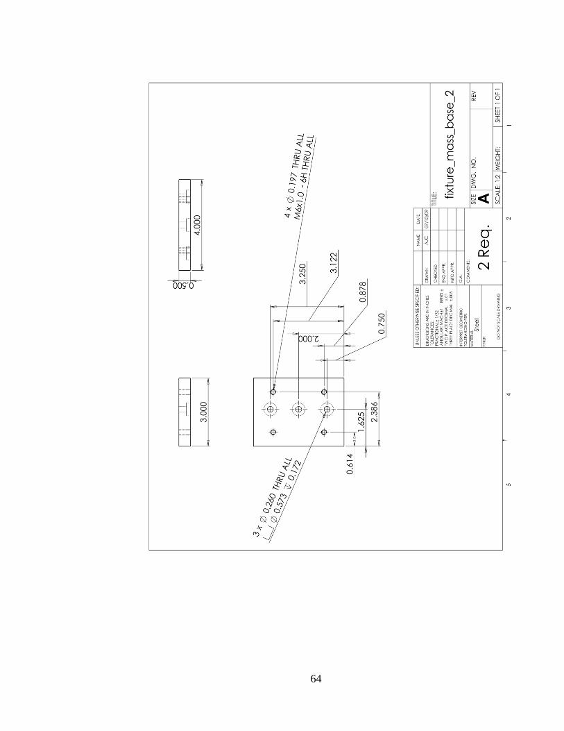
64

65

66

67

68

69

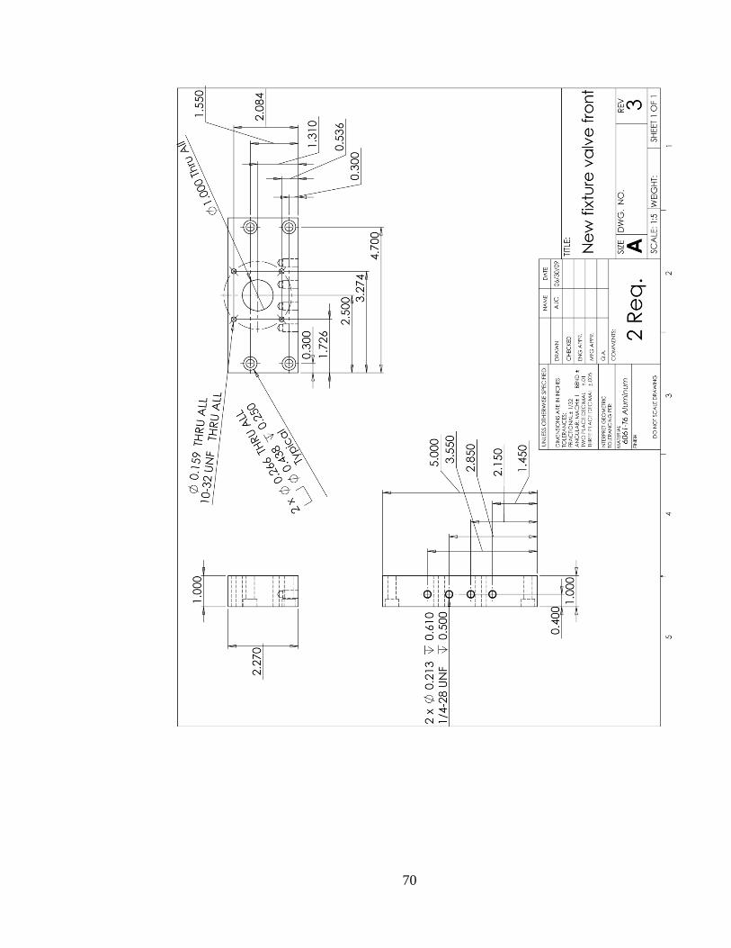
70

71

72

73

74

75

76

77

78

79

80

BIBLIOGRAPHY

Anderson, T. L. (1995). Fracture mechanics: fundamentals and applications. CRC Pr

I Llc.

Budynas, R. G., & Nisbett, J. K. (2008). Shigley's mechanical engineering design

(Vol. 10). McGraw-Hill.

Chelidze, D., & Cusumano, J. P. (2004). Identifying Multideminsional Damage in a

Hierarchial Dynamic System. Nonlinear Dynamics , 37 (4), 307-322.

Chelidze, D., & Cusumano, J. P. (2006). Phase space warping: nonlinear time-series

analysis for slowly drifting systems. Phil. Trans. R. Soc. A , 2495-2513.

Chelidze, D., & Liu, M. (2005). Dynamical Systems Approach to Fatigue Damage

Identification. Journal of Sound and Vibration , 281, 887-904.

Chelidze, D., & Zhou, W. (2008). Smooth orthogonal decomposition for modal

analysis of randomly excited systems. Journal of Sound and Vibration , 316, 137-

146.

Chelidze, D., Cusumano, J. P., & Chatterjee, A. (2002). A dynamical systems

approach to damage evolution tracking, Part 1: Description and Experimental

Application. Journal of Vibrations and Acoustics , 124 (2), 250-257.

Downing, S. D., & Socie, D. F. (1982). Simple rainflow counting algorithms.

International journal of fatigue , 4 (1), 31-40.

81

Farrar, C. R., Worden, K., Park, G., Todd, M., Nichols, J., Adams, D. E., et al. (2007).

Nonlinear system identification for damage detection. Technical Report LA-

14353, Los Alamos National Laboratory.

Fatemi, A., & Yang, L. (1998). Cumulative fatigue damage and life prediction

theories: a survey of the state of the art for homogeneous materials. Int. J. Fatigue

, 20 (1), 9-34.

Foong, C. H., Wiercigroch, M., & Deans, W. F. (2003). An Experimental Rig to

Investigate Fatigue Crack Growth Under Dynamic Loading. Meccanica , 38 (1),

19-31.

Foong, C.-H., Wiercigroch, M., & Deans, W. F. (2006). Novel Dynamic fatigue-

testing device: design and measurement. Measurements Science and Technology ,

2218-2226.

Fraser, A., & Swinney, H. (1986). Independent coordinates for strange attractors from

mutual information. Physical Reviews A , 33 (2), 1134-1140.

Galal, & Shawki. (1990). A reeview of fatigue testing machines. Engineering Journal

of Qatar University , 3.

Gu, M., Xu, Y. L., Chen, L. Z., & Xiang, H. F. (1999). Fatigue life estimation of steel

girder of Yangpu cable-stayed bridge due to buffeting. Jounal of Wind

Engineering , 383-400.

82

Hong, X., Mitchell, R. J., Chen, S., Harris, C. J., Li, K., & Irwin, G. W. (2008). Model

selection approaches for nonlinear system identification: a review. International

Journal of Systems Science , 925-946.

Jaksic, N., Foong, C.-H., Wiercigroch, M., & Boltezar, M. (2008). Parameter

Identification and modelling of the fatigue-testing rig. International Journal of

Mechanical Sciences , 20, 1142-1152.

Kantz, Holger, & Schreiber. (2004). Nonlinear Time Series Analysis. Cambridge:

Cambridge University Press.

Kennel, M., Brown, R., & Abarbanel, H. (1992). Determining embedding dimension

for phase-space reconstruction using a geometrical construction. Physical

Reviews A , 45 (6), 3403-3411.

Kerschen, G., Worden, K., Vakakis, A. F., & Golinval, J. (2006). Past, present and

future of nonlinear system identification in structural dynamics. Mechanical

Systems and Signal Processing , 505-592.

Lee, Y.-L., Pan, J., Hathaway, R., & Barkey, M. (2004). Fatugue Testing and

Analysis: Theory and Practice. Butterworth-Heinemann.

Ljung, L. (1987). System Identification: theory for the user. Prentice-Hall.

Mohammad, K. S., Worden, K., & Tomlinson, G. R. (1992). Direct parameter

estimation for linear and non-linear structures. Journal of Sound and Vibration ,

152 (3), 471-499.

83

Moon, F. C., & Holmes, P. J. (1979). A magnetoelastic strange attractor. Journal of

Sound and Vibration , 65 (2), 275-296.

Olsson, H., Astrom, K. J., Canudas de Wit, C., Gafvert, M., & Lischinsky, P. (1998).

Friction models and friction compensation. European Journal of Control , 176-

195.

Sanford, R. J. (2003). Principles of Fracture Mechanics. Prentice Hall.

Schreiber, T., & Schmitz, A. (1996). Improved surrogate data for nonlinearity tests.

Physical Review Letters , 77 (4), 635-638.

Sibson, R. (1985). Manual for the TILE4 Interpolation Package. University of Bath:

Department of Mathematics and Statistics.

Smith, R., & Hillmansen, S. (2004). A brief historical overview of the fatigue of

railway axles. Proceedings of the Institution of Mechanical Engineers, Part F:

Journal of Rail and Rapid Transit , 218 (4), 267-277.

Sonsino, C. M. (2007). Fatigue testing under variable amplitude loading.

Internattional Journal of Fatigue (29), 1080-1089.

Stephens, R. I., Fatemi, A., Stephens, R. R., & Fuchs, H. O. (2000). Metal Fatigue in

Engineering. Wiley-Interscience.

Surace, C., Worden, K., & Tomlimson, G. R. (1992). An improved nonlinear model

for an automotive shock absorber. Nonlinear Dynamics , 3, 413-429.

84

Worden, K., & Tomlinson, G. R. (2001). Nonlinearity in structural dynamics:

detection, identification and modeling. Institute of Physicd.