EAE 130B

Design Project Report

“Quarta Chord”

Daniel Pulache Alex Lee Alex Rivas Josh Pegadiotes Aaron Frisch

Abstract

The objective of this design project is to present the design of a low wing, two-seater training aircraft that is economical, lightweight, and low-cost to manufacture. The design is also expected to adhere to moderate performance parameters such as long airtime and moderate cruising velocity while still maintaining a long time before repair is needed. Using the Federal Aviation Administration’s (FAA) FAR Part 23 safety criteria to create a design space, we designed our aircraft following the ‘tried and true’ designs of comparable aircraft. This design was then put through several iterative processes to attain an optimal scenario and later tested through stability and performance algorithms. The result is an aircraft that successfully meets and surpasses the required design parameters. Our design integrates state of the art technologies which will modernize this aircraft and improve the capabilities of the pilot trainee, properly preparing them for the air travel industry. Recommendations for further design and development include further investigation into the structural analysis of the aircraft and the total lifecycle cost analysis.

i

Table of Contents

1.0 Introduction ...................................................................................................................................... 1

1.1 Design Purpose ............................................................................................................................. 1

1.2 Design Requirements .................................................................................................................... 2

2.0 Final Configuration............................................................................................................................ 3

2.1 Guiding Principles.......................................................................................................................... 3

2.1 Concept Evolution ......................................................................................................................... 4

2.2 Final Configuration ........................................................................................................................ 6

3.0 Propulsion System ............................................................................................................................ 8

3.1 Engine ........................................................................................................................................... 8

3.1.1 Engine Elimination.................................................................................................................. 8

3.1.2 Engine Performance ............................................................................................................... 9

3.2 Propeller ..................................................................................................................................... 11

3.2.1 Propeller Design .................................................................................................................... 11

4.0 Weight and Balance ........................................................................................................................ 15

5.0 Aerodynamics ................................................................................................................................. 18

5.1 Airfoil Selection ........................................................................................................................... 18

5.1.1 Elimination and Ranking Criteria ........................................................................................... 18

5.1.2 Natural Laminar Flow Airfoils ............................................................................................... 18

5.1.3 Options Considered .............................................................................................................. 19

5.2 Flaps ........................................................................................................................................... 22

5.2.1 Take-off and Landing Stages................................................................................................. 22

5.2.2 Flap Calculation .................................................................................................................... 22

5.3 Drag Breakdown ......................................................................................................................... 23

6.0 Stability and Control ....................................................................................................................... 25

6.1 Empennage Sizing ....................................................................................................................... 25

6.2 Stability and Control Analysis ...................................................................................................... 26

7.0 Aircraft Performance ...................................................................................................................... 28

7.1 Motivation .................................................................................................................................. 28

7.2 Methods ..................................................................................................................................... 28

7.2.1 Set Up .................................................................................................................................. 28

ii

7.2.2 Drag Force............................................................................................................................ 29

7.2.3 Stall Speed............................................................................................................................ 29

7.2.4 Take-Off and Landing Distances ........................................................................................... 29

7.2.5 Cruise Range ........................................................................................................................ 31

7.2.6 Climb Rates .......................................................................................................................... 31

7.3 Performance Characteristics ........................................................................................................ 32

8.0 Systems .......................................................................................................................................... 36

8.1 Cockpit Sizing ............................................................................................................................... 36

8.2 Landing Gear Configuration ........................................................................................................ 37

8.2.1 Landing Gear Analysis .......................................................................................................... 37

8.2.2 Design Choices ..................................................................................................................... 38

8.3 Avionics System........................................................................................................................... 40

9.0 Structures and Materials ................................................................................................................. 41

9.1 Material Selection ....................................................................................................................... 41

9.2 Structural Analysis ...................................................................................................................... 42

10.0 Cost .............................................................................................................................................. 44

11.0 Conclusions and Recommendations .............................................................................................. 46

11.1 Recommendations .................................................................................................................... 46

References ............................................................................................................................................ 47

1

1.0 Introduction

1.1 Design Purpose Most personal air vehicles (PAVs) in use today for recreation and pilot training were designed during the 1960s and 1970s. A combination of advances in understanding of aerodynamics and material technology allows for the design and development of aircraft in the 21st century which are more efficient. Nevertheless, there is a lack of state-of-the-art starter aircraft available today for beginning pilots. This lack of new small starter aircraft has led to increased running costs for pilot training schools and a decreased interest in flying.

There is a resulting need for new starter aircraft to train new pilots and create the excitement of flying an advanced, 21st century aircraft. These new aircraft must meet today’s design requirements: fewer emissions, reduced noise, minimal fuel consumption, and environmentally-friendly production. All this must be achieved while keeping the aircraft cost at a reasonable and competitive amount. Advances in aerospace engineering, such as the development of natural laminar flow airfoils, and advances in material science, such as the development of composite materials, allows for the design of aircraft which generate less drag and have reduced weight. Implementing these technologies into a new aircraft can yield a design which meets the challenging requirements and goals of the 21st century.

The goal of this report is to present the final design and configuration of a new small personal air vehicle (PAV) for use as a pilot training aircraft, which meets the demands of modern day design using the advanced technologies of the modern day. This report will present the requirements and goals of our PAV design. The final configuration is then presented along with the major design decisions made. Next, the report lays out the details of important aircraft components. The report also presents the aircraft design’s stability and performance characteristics. This report then presents a brief cost analysis of the design.

2

1.2 Design Requirements The design requirements for the aircraft, as presented in the request for proposals (RFP), are presented below.

Requirement Value Unit Cruise Speed 100 mph

Cruise Altitude 5,000 ft Cruise Distance 300 mi Service Ceiling 12,000 ft Total Payload 450 lbf

Cruise Fuel Consumption 5 gal/hr Take Off & Landing Distance 1,500 ft

In addition to the above requirements, the aircraft must

a. Be licensed as airworthy by meeting the Federal Aviation Administration Requirements (FAR) Part 23

b. Have a low-wing configuration c. Be powered by a single engine and propeller d. Be able to comfortably accommodate one and/or two pilots weighing between 90 and

225 lbs with heights between 5 and 6.5 ft without a ballast e. Fit in a 40 ft ‘T’ hangar with minimal effort f. Be equipped with typical basic VFR g. Be designed with ease of inspection and maintenance in mind

Table 1.1: Design Requirements

3

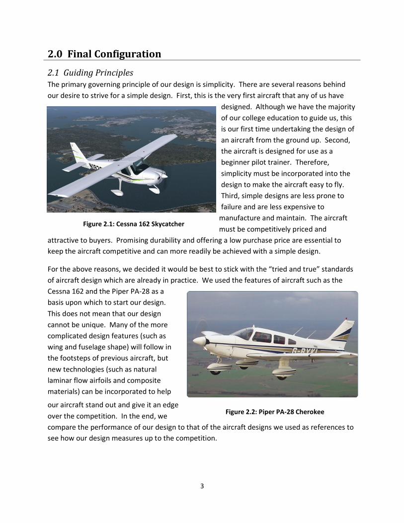
Figure 2.1: Cessna 162 Skycatcher

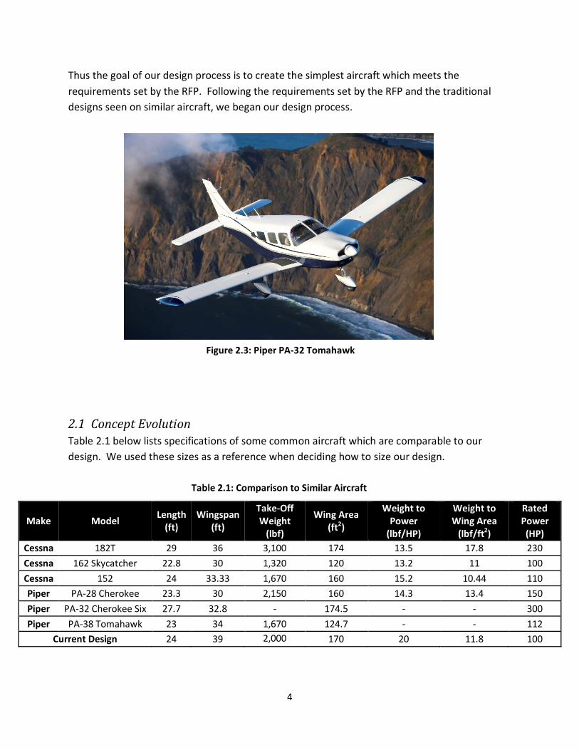
Figure 2.2: Piper PA-28 Cherokee

2.0 Final Configuration

2.1 Guiding Principles The primary governing principle of our design is simplicity. There are several reasons behind our desire to strive for a simple design. First, this is the very first aircraft that any of us have

designed. Although we have the majority of our college education to guide us, this is our first time undertaking the design of an aircraft from the ground up. Second, the aircraft is designed for use as a beginner pilot trainer. Therefore, simplicity must be incorporated into the design to make the aircraft easy to fly. Third, simple designs are less prone to failure and are less expensive to

manufacture and maintain. The aircraft must be competitively priced and

attractive to buyers. Promising durability and offering a low purchase price are essential to keep the aircraft competitive and can more readily be achieved with a simple design.

For the above reasons, we decided it would be best to stick with the “tried and true” standards of aircraft design which are already in practice. We used the features of aircraft such as the Cessna 162 and the Piper PA-28 as a basis upon which to start our design. This does not mean that our design cannot be unique. Many of the more complicated design features (such as wing and fuselage shape) will follow in the footsteps of previous aircraft, but new technologies (such as natural laminar flow airfoils and composite materials) can be incorporated to help

our aircraft stand out and give it an edge over the competition. In the end, we compare the performance of our design to that of the aircraft designs we used as references to see how our design measures up to the competition.

4

Figure 2.3: Piper PA-32 Tomahawk

Thus the goal of our design process is to create the simplest aircraft which meets the requirements set by the RFP. Following the requirements set by the RFP and the traditional designs seen on similar aircraft, we began our design process.

2.1 Concept Evolution Table 2.1 below lists specifications of some common aircraft which are comparable to our design. We used these sizes as a reference when deciding how to size our design.

Make Model Length

(ft) Wingspan

(ft)

Take-Off Weight

(lbf)

Wing Area (ft2)

Weight to Power

(lbf/HP)

Weight to Wing Area

(lbf/ft2)

Rated Power (HP)

Cessna 182T 29 36 3,100 174 13.5 17.8 230

Cessna 162 Skycatcher 22.8 30 1,320 120 13.2 11 100

Cessna 152 24 33.33 1,670 160 15.2 10.44 110

Piper PA-28 Cherokee 23.3 30 2,150 160 14.3 13.4 150

Piper PA-32 Cherokee Six 27.7 32.8 - 174.5 - - 300

Piper PA-38 Tomahawk 23 34 1,670 124.7 - - 112

Current Design 24 39 2,000 170 20 11.8 100

Table 2.1: Comparison to Similar Aircraft

5

One of the first steps of the design process is to set up the design space. Following the methods described in Ref 1, we created the design space shown in Figure 2.1 below. The design space was created by plotting several important design requirements at various cruise speeds and aircraft maximum lift coefficients. Thus, our design space allows us to graphically see how different cruise speeds and maximum lift coefficients affect the design. We decided to

keep our wing loading above 10 to reduce the effect of turbulence on the aircraft. We also

decided to maximize the weight to power ratio because a maximum will yield a

minimum take-off power. A small take-off power requires a less powerful engine, which usually means a cheaper and more fuel efficient engine.

The take-off weight and design point used for our design were iterated several times. The take-off weight was selected based on the take-off weight of similar aircraft, which can range from 1,600 lbs to 2,200 lbs. Our final chosen take-off weight is 2,000 lbs and design point is

= 20 and = 11.8. These values yield a take-off power of 푃 = 100 퐻푃 and

wing area 푆 = 170 푓푡 .

Approximate Design Point

Figure 2.1: Design Space

6

Table 2.2: Final Configuration

2.2 Final Configuration Our final aircraft configuration (shown on the next page) calls for a conventional wing layout (main wing in front of tail wing) with rectangular-shaped wings. The main wings have no sweep or taper, but do have some dihedral. The dihedral is necessary to maintain stability, since the aircraft must have a low-wing configuration. The aircraft is equipped with the standard control surfaces: two ailerons, two elevators, and a rudder. The main wing is equipped with two trailing-edge flaps to help generate lift on take-off and landing. The empennage has the standard twin horizontal tails with one vertical tail in the middle. The aircraft is equipped with a single air-cooled engine and a two-bladed propeller in tractor configuration. The aircraft is equipped with fixed landing gear covered by pants to reduce drag. A dimensioned three-view of our model is shown on the next page. The table below provides key parameters of the final design.

Parameter Value Description 푊푃 11.8 Weight-to-Power Ratio 푊푆 20 Weight-to-Wing Area Ratio

푊 2,000 lbf Takeoff Weight 푆 170 ft2 Wing Area 푃 100 HP Maximum Takeoff Power 퐴푅 9 Aspect Ratio 푏 39 ft Span 푐 4.34 ft Chord (constant) 푉 150 mph Cruise Speed ℎ 5,000 ft Cruise Altitude

7

2.5 1.97

5.74

24

5.42

10

2

39

4.34

4.17

6

4.65 5.33 9.05

0.5

4.67

Note: All dimensions in feet

5.5

2

8.17

8

3.0 Propulsion System

3.1 Engine

3.1.1 Engine Elimination

The choice of power plant for our design is based on our design point of = 20 .

Since our take-off weight is 2,000 lbs, our engine must have a rated power of 100 HP to satisfy the design point. This is a very commonplace power rating for general aviation engines, which made for a variety of choices that were available to us.

There were three main engines that we inspected to find the best choice for our aircraft. The first motor is the Lycoming O-235. This engine is used in the Cessna 152, which is a well-known single engine aircraft which has been around since the mid twentieth century. It is an outdated and old design which does not keep up with our performance parameters. In the Lycoming O-235 User Manual, at the ‘economy cruise’ power setting, the engine performs at 75 HP and 2250 RPM with a fuel consumption of 7.3 gal/hr. However, our maximum fuel consumption is 5.0 gal/hr. This is an important requirement due to this aircraft’s role as a trainer, since it will see extended periods of airtime and cannot use as much fuel as the Lycoming O-235 requires.

The next engine is the Firewall Forward CAM 100. This engine is much newer than the Lycoming and is a little more efficient, coming from the derivative of a Honda Civic motor platform. This engine is exclusively liquid cooled, which requires an additional liquid coolant storage bay. This would add to the overall weight of our aircraft design. This engine also produced more power than its Lycoming counterpart during cruise, boasting 80 HP at 4500 RPM with a fuel consumption of 6.16 gal/hr. This fuel consumption rate is an improvement from the Lycoming, but is still above our limit of 5.0 gal/hr. This engine turned out to be a better choice for our design, but is still not ideal due to its fuel consumption rate.

The next engine is the Rotax 912 iSc, another derivative of a Honda motor applied to aviation. This engine is produced by a very noteworthy propulsion company which produces very efficient, powerful platforms for general aviation purposes. This engine showcases an astonishing fuel consumption of just 4.3 gallons per hour at 5000 RPM and 83 HP. This is a significant fuel consumption rate improvement to the other two competition motors. Since the Rotax 912 iSc satisfies both our power and fuel consumption requirements, we chose this engine for our design. The details of this engine are presented in the next section and provide further reason for this engine’s use on our aircraft.

9

3.1.2 Engine Performance The plot below shows the relationship of engine power performance, RPM, and torque generated.

The operation window that we are interested in for cruise is around 80 HP or 60 kW. In this figure, 60 kW corresponds to an engine speed of 5,000 RPM and 60 NM of torque at the propeller flange. This correlates to our 75% power scenario at cruise conditions. In the figure below, we see that this power output comes with a fuel consumption of 4.3 gallons per hour.

Figure 3.1: Engine Power vs RPM (Ref. 19)

10

Again, we are operating at 5,000 RPM which corresponds to 16 liters per hour of fuel, which converts to 4.3 gallons in British units. This specific model is the iSc, which is FAA certified and comes outfitted with fuel-injected cylinders and an onboard electronic engine management computer, which are advancements in technology which will extend the life of the engine as well as help modernize our overall aircraft design.

Since this engine can produce as high as 5,800 RPM, there is a reduction gear of 1:2.43 on the propeller shaft. This retards the speed of the shaft such that a propeller will be able to safely mount to the engine and operate in a regime of RPMs which is realistic and safe for the propeller.

This engine is relatively compact, measuring only 22.1 inches long, by 22.7 inches wide and 28.2 inches tall. This makes for a simple mounting procedure where the engine will be bolted to hardpoint struts in the nose of the aircraft.

In addition to its incredible fuel efficiency, this motor also contains a two-part cooling system. It uses a combination of liquid and air cooling to maintain ideal operational engine temperature for the aircraft. This motor contains a liquid-cooled system for the cylinder heads, run by a sump pump hardlined into the cam gear, coupled with an air-cooled cylinder system. This is a useful innovation because the cylinder heads on an aircraft engine are a critical location in the cylinder which is integral to proper engine performance and needs its temperature to be under very careful control. With the liquid-cooled system,

Figure 3.2: Engine Fuel Consumption vs RPM (Ref. 19)

11

the heat from combustion will be very efficiently wicked away, decreasing the chance of malfunction during operation. At the same time, this engine also utilizes air-cooling for the bulk of the cylinder cooling. This is beneficial because liquid-cooling can quickly become detrimental due to the weight of the coolant needed for operation. The air-cooling allows for lightweight, efficient cooling of the remaining engine parts.

In the end we decided to go with the Rotax 912 iSc motor due to its efficiency benefits, along with its ideal power output, innovative thermal control, and relatively low price of $18,578.00 USD.

3.2 Propeller

3.2.1 Propeller Design For our design, we chose to use a single, two-bladed propeller for the propulsion of our airplane. This trainer airplane is a relatively small two-seater single engine airplane, so propeller driven propulsion is the obvious fit. A fixed pitch propeller will be used since there is no substantial benefit for a variable-pitched propeller due to the low air speeds and required performance of the airplane. Fixed-pitch design also reduces cost in both parts and lifetime maintenance. Using blade-element theory along with momentum theory as fundamentals for the design, a MatLab code was written to design the propeller blades. We re-designed the propeller to meet the specified design requirements outlined in the RFP and to match our newly chosen engine: the Rotax 912 iSc. Maximum propulsive efficiency was once again a large consideration in order to limit the fuel consumption of the airplane while still producing the required thrust at cruise. The final propeller design is a two-bladed configuration and was found by changing the blade shape until the propeller matched both the engine power output at cruise and the required thrust force cruise. The propeller blade shape and pitch distribution were optimized for cruise conditions at a cruise speed of 150 mph and an altitude of 5,000 feet. Our approach to the design of the propeller blades involved choosing a chord distribution and calculating the resulting lift distribution along the blade. Many iterations were performed to determine the best blade shape which could match our new engine power output and generate enough thrust to match the drag force at cruise. These iterations were performed based on refined data from our engine group and aerodynamics group. The Sensenich propellers used on many Cessna 152s and Piper Tomahawks were used as a

12

reference for this process. The blade angles were determined using the optimum blade loading Betz condition. The Betz limit is the maximum energy and therefore the maximum power that can be extracted from the oncoming wind. After many iterations of the propeller shape, we were able to come up with a reasonable propeller to match the Rotax 912 iSc and perform as required. The planform shape of the final propeller design is shown below, along with the sectional coefficient of lift distribution.

Figure 3.3: Blade Planform View (with and without twist)

Figure 3.4: Propeller Sectional Lift Distribution

13

3.3.2 Propeller Performance Table 3.1 below summarizes our propeller’s performance at cruise

Table 3.1: Propeller Properties at Cruise Number of Blades

2 Cruise RPM 2058 RPM

Propeller Diameter

6 ft Aircraft Drag 110 lbf

Cruise Velocity 150 mph Propeller Thrust 115 lbf CL,design 0.2571 Required Power at Cruise 83 HP Activity Factor 194 Percent Total Engine Power 75% PTO

Advance Ratio 1.07 Fuel Consumption 4.3 gal/hr Through our propeller design process, we were able to produce an efficient propeller that generated the required thrust at cruise. Our newly refined drag analysis on the airplane shows that there will be approximately 110 lbf of total drag acting against the forward motion of the aircraft at a cruise speed of 150 mph. At the same cruise conditions, the propeller produces around 115 lbf of thrust, allowing the aircraft to remain in steady, level flight. The figures below provide the engine horsepower and required propeller thrust matching conditions.

Figure 3.5: Engine-Propeller Matching Conditions

14

Figure 3.6: Thrust vs. Propeller RPM

Our new engine, the Rotax 912 is equipped with a gear reduction mechanism. The gear box has a 1:2.43 ratio on the propeller shaft. The propeller shaft RPM is reduced from the engine RPM, allowing the engine to operate within a range of allowable fuel consumption. The engine power at 5000 RPM and 5,000 feet is around 80 HP. This engine RPM corresponds to a propeller RPM of 2058. We were able to match the required horsepower for the propeller with the engine power.

Figure 3.7: Efficiency, Thrust Coefficient, and Power Coefficient vs. Advance Ratio

15

With our current propeller design, cruising at 150 mph and 5000 engine RPM, corresponds to an advance ratio of 1.07. As seen in Figure 3.7, we have around 90% propulsive efficiency at the cruise advance ratio. This will be extremely beneficial in terms of fuel consumption and ultimately overall cruise range. Lastly, the propeller will be manufactured from aluminum alloy, similar to what is currently used for the Sensenich propellers. Aluminum alloy is very light and exceptionally strong relative to its weight. Even more importantly, aluminum alloy will not corrode. This will provide many hours of use without the hassle of replacing or repairing the propeller.

4.0 Weight and Balance The airplane’s weight is an extremely important parameter which is crucial to its ability to fly. Not only are the component weights crucial to the airplane getting off the ground, they also contribute to its ability to maneuver in flight and to be controllable. The component weights were determined based on similar airplane component weights along with material density, surface area, and volume. The weight breakdowns for three configurations are tabulated below.

Max Take-Off Weight Operating Empty Weight Empty Weight

Component Weight (lbs) Percent of Total Weight (lbs) Percent of Total Weight (lbs) Percent of Total

Fuselage 450 22.7% 450 24.3% 450 32.0%

Main Wing 310 15.7% 310 16.7% 310 22.1%

Empennage 77.6 3.9% 77.6 4.2% 77.6 5.5%

Propeller 26.28 1.3% 26.28 1.4% 26.28 1.9%

Air Intake 32.5 1.6% 32.5 1.8% 32.5 2.3%

Landing Gear 124 6.3% 124 6.7% 124 8.8%

Pilots 450 22.7% 450 24.3% 0 0.0%

Engine Weight 260 13.1% 260 14.0% 260 18.5%

Fixed Equipment 125 6.3% 125 6.7% 125 8.9%

Fuel 125 6.3% 0 0.0% 0 0.0%

TOTAL 1980.38 100.0% 1855.38 100.0% 1405.38 100.0%

The aircraft components were placed in and on the airplane in a configuration with the center of gravity (CG) in mind. The pilot and luggage weights were key parameters due to their variation for different flight scenarios. The airplane must be stable for a variety of loading

Table 4.1: Maximum Take-Off Weight Component Breakdown

16

scenarios, from the required 450 pound payload with maximum fuel down to one 90 pound pilot flying on just the fuel reserves (~ 25 lbs). In order to account for these variations, the pilot seats were aligned nearest to the centerline of the aircraft so as to limit the induced lateral moment about the center of the aircraft. The aircraft’s center of gravity excursion throughout flight envelope and for various loading scenarios is shown below.

Figure 4.1: Aircraft Center of Gravity Excursion Diagram

In order to calculate the center of gravity locations, the individual components had to be placed on the airplane in their respective locations. Our method for component CG locations was carried out using the NASA Vehicle Sketch Pad program (VSP). Individual components such as the engine, main wing, landing gear, fixed equipment, and empennage were added to the aircraft in VSP as point masses. These point masses represented the center of gravity of each component. From here, VSP was able to calculate the total configuration’s center of gravity. Fuel and payload were also added in their respective locations. The payload weight was specified in the RFP as maximum 450 lbs while our required fuel weight was calculated based on the range requirement of the airplane. Weights of the fuel and payload were varied to represent fuel reserve and lightweight pilot loading scenarios. Aircraft CG locations were then calculated for each scenario. The following figure shows the component CG locations along the fuselage of the airplane, represented by the thick solid blue line.

70 80 90 100 110 120 130 140 150 1601300

1400

1500

1600

1700

1800

1900

2000

2100

Location from Tip of Spinner (inches)

Wei

ght (

lb)

Center of Gravity Excursion

Max Take-OffEmptyOne 90-lb Pilot, Full FuelReserve Fuel (25lbs), Two 225lb PilotsReserve Fuel (25lbs), One 90lb PilotLeading EdgeTrailing EdgeCG Location

17

Figure 4.2: Aircraft Component CG Locations

Table 4.2: Static Margin for Various Loading Scenarios

Loading Scenario Payload Weight Fuel Weight Static Margin (%)

Max Take-Off 450 lbs 150 lbs 13

Max Payload, Fuel Reserve 450 lbs 50 lbs 16.5

Light Payload, Fuel Full 90 lbs 150 lbs 3.7

Light Payload, Fuel Reserve 90 lbs 50 lbs 7.5

Empty 0 lbs 0 lbs 5.6

The static margin values were also obtained through the “Aero Reference” mode in VSP. The static margin is the distance between the center of gravity and the airplane’s total aerodynamic center including empennage. The CG of the airplane must be in front of the aerodynamic center for the airplane to be longitudinally stable. At maximum take-off weight our airplane has a static margin of 13 %. We believe this is a reasonable margin and will provide a stable aircraft that is easy to fly yet still maneuverable in flight.

18

5.0 Aerodynamics

5.1 Airfoil Selection Airfoil selection began by first determining the target CL at cruise. This is the CL necessary to keep the aircraft in level flight during cruise. The CL at cruise is given by

퐶 =푊

12휌푉 푆

(5.1)

At 5,000 ft altitude, 150 mph, and assuming maximum takeoff weight, our design 퐶 is 0.2381. The second important parameter to consider when selecting an airfoil is the design Reynold’s Number. The Reynold’s Number (Re) is given by

푅푒 =푉 푐

휇

(5.2)

where 푐 is the chord and 휇 is the kinematic viscosity. A wing which has a varying chord along its span will have a different design Re at different points along the span. For simplicity, we chose a rectangular wing shape. As a result, our wing has a constant Re along the span of the wing. Our design Re (at cruise) is 6.54x106.

5.1.1 Elimination and Ranking Criteria Any airfoil which cannot produce the target CL at a low incidence angle will produce an unnecessary amount of drag during cruise. Larger incidence angles lead to more lift, but also cause an increase in drag. Any airfoil which cannot produce the desired CL at cruise at a low incidence angle is immediately eliminated.

The airfoils which can produce the target CL at a low incidence can be ranked based on their drag coefficient, CD, at the target CL. The airfoil which has the lowest CD at the target CL becomes the winning design.

5.1.2 Natural Laminar Flow Airfoils Particular interest was paid to natural laminar flow (NLF) airfoils. Typical airfoil design used to assume fully turbulent flow over the airfoil. It was assumed that this turbulent (faster) flow would yield higher lift. While this design approach did yield airfoils which could produce more lift, the airfoils suffered from large drag coefficients (Ref. 5). For this reason,

19

research began to focus on laminar flow airfoils. The objective of designing laminar flow airfoils is to maintain laminar flow over as much of the airfoil’s surface as possible, while still maintaining the necessary lift coefficients. If successful, the laminar flow will support the aircraft while causing far less drag than turbulent flow (Ref. 5).

A notable design feature of NLF airfoils is their apparently blunt and thick leading edge. This leading edge is designed to cause the point of transition from laminar to turbulent flow to move slowly toward the leading edge. In contrast, the transition point on typical NACA 6-series airfoils would move rapidly toward the leading edge, causing increased drag (Ref. 4). The blunt leading edge of NLF airfoils allows for a steady transition to turbulent flow and a high maximum lift coefficient (Ref. 4).

A primary concern of NLF airfoils is that if laminar flow is not achieved along a significant portion of the airfoil, large increases in drag may result. Damage to the wing and/or foreign objects on the wing (i.e. dirt, insect remains) may cause a more rapid transition to turbulent flow and ruin the performance of the wing. Experiments on a NLF airfoil (see Ref. 6) proved that the drag performance of the NLF airfoil suffered considerably when laminar flow was not achieved. However, considerable damage or other alterations to the airfoil would have to be present to prevent laminar flow from being achieved. Tests on a NLF airfoil (see Ref. 6) proved that even when a roughness strip was placed near the leading edge, laminar flow was still achieved and the maximum lift coefficient only decreased by about 0.04.

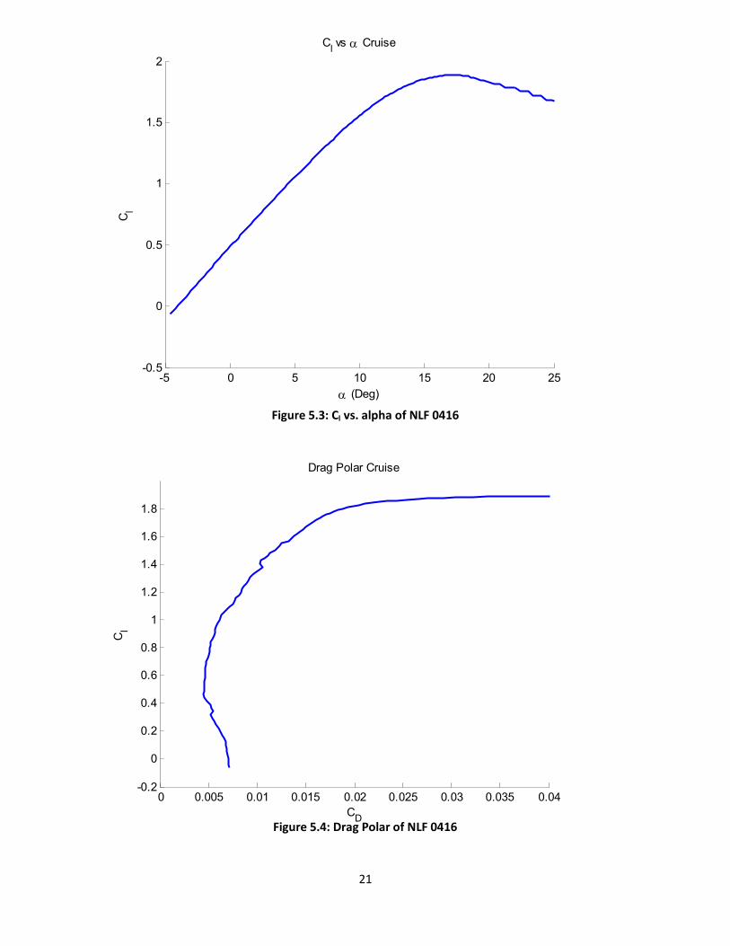
5.1.3 Options Considered Several NACA 6-series airfoils and NLF airfoils were evaluated using XFOIL, a 2D airfoil performance evaluation software. The drag polars generated by the program demonstrated the superiority of the NLF airfoils, every NLF airfoil generated less drag at our design CL than the NACA 6-series airfoils. Our final selection was reduced to three NLF airfoils: the NLF 0215f, the NLF 0414f, and the NLF 0416. The drag polars for these airfoils at a Reynold’s Number of 6.54x106 are presented below. These drag polars have been enlarged to show the range of 0 < CD < 0.04 in more detail. Table 5.1 below lists some important characteristics of the considered airfoils. Some of the data for the NLF 0215f is missing because the data from the XFOIL program did not converge at certain incidence angles. However, the trends can be seen in the following figures.

Table 5.1: Comparison of Airfoil Characteristics

푪푫 퐚퐭 푪푳,풅풆풔풊품풏 휶 퐚퐭 푪푳,풅풆풔풊품풏 푪푳,풎풂풙 휶 퐚퐭 푪푳,풎풂풙 NLF 0215f N/A N/A 1.9032 21.2o

NLF 0414f 0.00409 -2.4 o 1.9677 20o

NLF 0416 0.0057 -2.1o 1.8897 17.2o

20

-5 0 5 10 15 20 25-0.5

0

0.5

1

1.5

2

(Deg)

Cl

Cl vs Cruise

NLF0416NLF0414fNLF0215f

0 0.005 0.01 0.015 0.02 0.025 0.03 0.035 0.04-0.2

0

0.2

0.4

0.6

0.8

1

1.2

1.4

1.6

1.8

CD

Cl

Drag Polar Cruise)

NLF0416NLF0414fNLF0215f

Figure 5.1: Cl vs. alpha of Potential Airfoils

Figure 5.2: Drag Polar of Potential Airfoils

21

-5 0 5 10 15 20 25-0.5

0

0.5

1

1.5

2Cl vs Cruise

(Deg)

Cl

0 0.005 0.01 0.015 0.02 0.025 0.03 0.035 0.04-0.2

0

0.2

0.4

0.6

0.8

1

1.2

1.4

1.6

1.8

Drag Polar Cruise

CD

Cl

Figure 5.3: Cl vs. alpha of NLF 0416

Figure 5.4: Drag Polar of NLF 0416

22

5.2 Flaps In order to take-off and land, we needed to consider increasing our 퐶 at angles of incidence that are appropriate for take-off and landing. The 퐶 required in order to meet the take-off distance requirement is 1.9. In order to take-off, we must achieve this target 퐶 . Our airfoil does not generate this 퐶 even at high incidence angles, thus flaps were considered in our design. The flap design considered is a plain trailing edge flap.

5.2.1 Take-off and Landing Stages Takeoff and landing each have a target 퐶 which we must satisfy in order to take-off and to land. Take-off has four different stages: Acceleration, Rotation, Take-Off, Climb 50 ft. Throughout these stages, the flaps of the airplane are deployed at a constant angle. During the Acceleration stage the airplane starts from rest up to its take-off speed and the wing remains at its installed angle of attack of -2.1o. During its Rotation stage, the airplane maintains its take-off speed while rotation up to an incidence angle of 8o. During the take-off stage, the airplane’s incidence angle remains at 8o. It is at this point when the airplane finally leaves the ground. The last stage finishes when the airplane has climb 50 ft. Landing can be broken down into four stages, just like take-off, but in reverse order.

5.2.2 Flap Calculation The flaps will be deployed to its desired flap deflection throughout the entire landing and take-off process. From this, it is known that the flaps must be designed in order to increase the global 퐶 at 8o incidence since this is the incidence angle at which the airplane is actually taking-off and landing. The ∆퐶 needed at take-off and landing is 1.9 and 2.28 respectively.

Following Ref. 3, the flaps for our airplane were chosen to be plain trailing edge flaps. The required change in lift coefficient, ∆퐶 , can be found using

Δ퐶 = 훿퐶

(퐶 ) (퐶 ) 푘′ (5.3)

where 훿 is the flap deflection, 퐶 accounts for the flap size to thickness ratio, and 푘′ is a

correction factor which accounts for the non-linearities at high flap deflection. Using this equation we can find the flap deflection and flap size according to our target ∆퐶 . Using Figures 8.13, 8.14, and 8.15 in Roskam, we were able to come up with the correct values for the flap deflection equation. A MatLab code was written in order to do the calculation. The table below lists our results.

23

Main Wing38%

Fuselage15%

Horizontal Tail Wings

5%

Vertical Tail Wing

4%

Landing Gear8%

Protuberances4%

Misc Drag3%

Induced (Cruise)23%

Drag Breakdown at Cruise

Table 5.2: ∆푪풍 and Flap Calculation for 풄풇풄

= ퟎ.ퟑ

Flap Deflection (휹풇) ∆푪풍 10o 0.7467 11o 0.8049 12o 0.8601 13o 0.9124 14o 0.9617 15o 1.0080 16o 1.0513 17o 1.0916

Because this is the local ∆퐶 and not the global coefficient of lift we must take into account

that this value will decrease when we add it to the global 퐶 . A (ratio between chord of

the flap and chord of the airfoil) of 0.3 was chosen to satisfy the ∆퐶 requirement at both takeoff and landing. A flap deflection of 10o is required for the airplane to take-off and a flap deflection of 17o is required to land. The flaps can deflect more than this if necessary in order to take off faster or land at a slower speed.

5.3 Drag Breakdown A simple drag breakdown was performed following Ref. 1, based on the drag performance of similar aircraft. The drag breakdown is tabulated and presented graphically below. The zero-lift drag components are not analytical, but are estimates based on comparable aircraft.

Figure 5.3: Drag Breakdown at Cruise

24

50 100 150 200 250 3000

50

100

150

200

250

300

Speed (mph)

Dra

g Fo

rce

(lbf)

Drag versus Airspeed

Lift Induced DragParasitic DragTotal Drag

Drag Component CD Percent Main Wing 0.0050 38.17% Fuselage 0.0020 15.27%

Horizontal Tail Wings 0.0006 4.58% Vertical Tail Wing 0.0005 3.82%

Landing Gear 0.0011 8.40% Protuberances 0.0005 3.82%

Misc Drag 0.0004 3.05% Zero-Lift Drag, CD0 0.0101 77.10%

Induced Drag 0.0030 22.90% Total Drag 0.0131 100%

The plot of drag versus airspeed shows that our design reaches its minimum drag between 100 and 150 mph. At our cruise speed of 150 mph, the aircraft experiences a drag force of 110 lbf.

Table 5.2: Detailed drag breakdown at cruise conditions

Table 5.4: Drag Force vs Airspeed (5kft Altitude)

25

6.0 Stability and Control

6.1 Empennage Sizing The empennage is the control center of the aircraft. The vertical tail needs to be large enough to be able to maintain yaw authority during flight while at the same time not being so large that it will impart an adverse rolling moment on the airframe. As with the vertical tail, the horizontal tail must be large enough to maintain pitch authority for the aircraft.

For the sizing of the empennage surfaces, we chose to start by modeling our tail panels after those of similar aircraft. With these choices, we then dimensioned out the empennage based upon the method outlined by Ref. 2. These dimensions and values were then analyzed via rudimentary static stability analysis to fine-tune them into an optimized stabilization system.

The sizing of the control surfaces followed a similar procedure, beginning with the reference to similar aircraft, followed by the analysis of the moments created by the empennage and basic hypothetical side-slip scenarios to find the best configuration of the control surfaces on the wing and empennage to insure that the pilot(s) of this aircraft would not lose control during flight. For the elevator, we needed to insure that it could effectively control the pitch attitude of the aircraft. To do this, we chose to orient the elevators along the entirety of the span of the tail, so as to insure an even distribution of the lifting so that a rolling moment was not created. The same approach was taken for the rudder on the vertical tail. We stretched the entire span of the vertical stabilizer with the rudder, so as to make sure the rudder effectively controlled the yaw attitude. The ailerons were placed distal to the flaps on the main wing to ensure that they would continue to function if the wing were to begin to stall in order to maintain roll authority throughout the flight. The ailerons were also placed close to the wingtips so that they would create a large rolling moment with low input angle.

The tail volume coefficient is an important tool used to help size the empennage surfaces along with place the center of gravity for the aircraft. The tail volume calculation is carried out with a tail arm selection already in mind. The tail volume is computed as follows:

푇푎푖푙 푉표푙푢푚푒 =푇푎푖푙 퐴푟푒푎푊푖푛푔 퐴푟푒푎

푇푎푖푙 퐴푟푚퐴푣푔.푊푖푛푔 퐶ℎ표푟푑 (6.1)

Table 6.1 below lists the sizes of our control surfaces. The aileron control surface area over the wing area is 0.08.

26

6.2 Stability and Control Analysis The stability and control of an aircraft is one of the many crucial characteristics which must be satisfactory in any airplane design. Stability of the airplane starts with the longitudinal static stability. A statically stable aircraft is one which tends to return to its equilibrium state after perturbations to the aircraft. This means that if the airplane is disturbed away from the equilibrium angle of attack, moments are generated about the center of gravity that tend to return the airplane to equilibrium. For this to be achieved, the pitching moment must be opposite to that of the induced angle of attack due to acting forces. For example, when the angle of attack is increased due to a gust of wind, the airplane must generate a negative pitching moment (nose down) to return back to an equilibrium state. This of course is taking into account no elevator input or any other control inputs. This corresponds to a negative pitching moment coefficient slope: Cm,α. The following figure represents the moment coefficient slope for our proposed design.

Vertical Tail Horizontal Tail

Volume 0.08 Volume 0.80

Area 20 ft2 Area 20 ft2

Height 5.74 ft Height -

Base Length 4.467 ft Length 10 ft

Tip Length 2.5 ft Width 2 ft 푹풖풅풅풆풓 푨풓풆풂푻풐풕풂풍 푨풓풆풂 0.42

푬풍풆풗풂풕풐풓 푨풓풆풂푻풐풕풂풍 푨풓풆풂 0.50

Table 6.1: Control Surface Sizes

27

Figure 6.1: Pitching Moment vs. α

As seen in Figure 6.1, we do in fact have a negative pitching moment slope—that is to say

< 0. This shows that the aircraft is statically stable and will tend to return to equilibrium

in the case of any disruptions to the flight path. Figure 6.1 also shows our trim angle for installation of the main wing. The angle at which zero moment is produced about the center of gravity is the angle at which we want to cruise in level flight. This corresponds to a main wing trim angle of around -2°.

Along with trimming the main wing, our proposed design also requires a trim angle for the horizontal tail wing. Since our center of gravity locations are a very large percentage of the mean aerodynamic chord (MAC), the center of gravity (CG) is aft of the center of pressure—the location of the lifting force on the main wing. This requires the tail wing to produce an upward lifting force to create a balanced aircraft. In order to have a lifting tail at cruise conditions, the tail wing will be trimmed at an angle to produce the necessary lifting force. Taking into account the tail airfoil, the NACA0014, the moment arm between the CG and the tail aerodynamic center, and CL,α of the tail and main wings, we were able to make some initial calculations for the trim angle of horizontal tail. It was calculated that a trim angle between 3-5° will be sufficient to produce the required lift while still maintaining its elevator pitch authority.

Approximate Trim Angle (~ -2°)

28

7.0 Aircraft Performance

7.1 Motivation Exceptional aircraft performance statistics are essential for success when selling an aircraft design. Individual component performance is important and incorporating modern technology can make the aircraft more appealing, but ultimately the various components and systems of the aircraft must come together to demonstrate that the aircraft as a whole has a sound and competitive design. Evaluating the aircraft’s performance will often end in iteration, requiring the designers to change design features in order to improve the aircraft’s performance characteristics. The aircraft performance stage is a reality check which ensures that the design meets the minimum performance requirements and has competitive performance characteristics. The aircraft performance characteristics are calculated as described in Section 7.2 below.

7.2 Methods

7.2.1 Set Up In order to perform our aircraft performance analysis, we first set up a mock flight path for the aircraft to simulate the different stages of flight. The table below displays the flight path used for our aircraft performance analysis.

Phase Take Off Climb Cruise Loiter Descent Landing Shut Down Final Weight

Weight Ratio 0.993 0.992 0.949 0.998 0.993 0.996 0.995 - Weight (start of phase)(lbf) 2000 1,986 1,970 1,870 1,866 1,853 1,845 1,836

The weight ratios in Table 7.1 above are estimates based on common weight ratios for single engine, propeller-driven aircraft given by Ref. 1. The weight ratios represent changes in weight due to burning fuel. The weight ratios can be adjusted to simulate burning more or less fuel at each stage. For example, the weight ratio for the cruise phase was adjusted until the total fuel burned reached the 100 pounds that we allotted for fuel.

Table 7.1: Mock Flight Stages

29

7.2.2 Drag Force The total drag force is given by

퐷 =12퐶 휌푉 푆 = 퐷 + 퐷 (7.1)

Where 퐷 is the zero-lift or form drag and 퐷 is the lift-induced drag. The zero-lift drag coefficient is an estimate given in Table 5.2. The lift-induced drag coefficient is given by

퐶 , =퐶

휋 ∙ 퐴푅 ∙ 푒 (7.2)

Where 푒 is the Oswald’s Efficiency. We assumed a constant Oswald’s Efficiency of 60% based on common values for other aircraft.

7.2.3 Stall Speed The stall speed can be found using the definition of the lift coefficient:

퐶 =퐿

12휌푉 푆

→ 푉 =퐿

12퐶 휌푆

(7.3)

The aircraft will stall when the forward velocity, 푉, is low enough to prevent to prevent the generation of sufficient lift force. It may be assumed that lift equals weight when performing this calculation. When the substitution 퐿 = 푊 is made into equation (7.3), we know that any speed less than the resulting value will not be fast enough to keep the aircraft in the air.

7.2.4 Take-Off and Landing Distances The take-off distance of our design is calculated using a 퐶 , of 1.9, as suggested by our

design space. The Oswald’s efficiency, 푒, is increased to 0.8 to account for ground effect. If 푉 is the stall speed, then the liftoff speed can be estimated by

푉 = 1.1푉 (7.4)

The total takeoff distance is composed of four stages: ground distance, 푆 , rotation distance, 푆 , transition distance, 푆 , and climbout distance, 푆 . If the aircraft lands on a

30

level runway in zero wind, then the ground distance can be found from a force balance. The resulting equation is

푆 =푊푔

푉푑푉(푇 − 휇푊)− (퐶 − 휇퐶 ) ∙ 0.5 ∙ 휌푉 푆

(7.5)

where 휇 is the friction coefficient between the ground and the aircraft. The rotation distance is

푆 = 푡 푉 (7.6)

where 푡 is the time it takes the aircraft to rotate to the climbout angle (usually 1 to 3 seconds). The transition stage is where the aircraft finally leaves the ground, thus the aircraft gains both distance, 푆 , and altitude, ℎ :

푆 = 푅 ∙ sin훾 (7.7)

ℎ = 푅(1− cos훾 ) (7.8)

The climbout angle, 훾 , is given by

훾 = sin푇푊−퐶퐶

(7.9)

The term 푅 is the radius of curvature that the aircraft follows at it takes off and is dependent upon the number of G’s, 푛, that the aircraft can safely handle at takeoff.

푅 =푉

푔(푛 − 1) (7.10)

Finally, the aircraft continues to gain altitude until the required altitude for the completion of takeoff is reached. For our design, the aircraft must reach 50 ft to complete take off.

푆 =ℎ − ℎ

tan 훾 (7.11)

The total landing distance is the sum of the ground roll, rotation distance, transition distance, and climbout distance.

The landing performance is governed by two important speeds: the approach speed, 푉 , and the touchdown speed, 푉 . These speeds can be estimated by

푉 = 1.3푉 (7.12)

푉 = 1.15푉 (7.13)

31

The landing distance is composed of the air distance, 푆 , the free roll distance, 푆 , and the braking distance, 푆 . The air distance is the distance the aircraft travels forward while still in the air. By performing an energy balance, the air distance can be found:

푆 =푊퐹

푉 − 푉2푔

+ ℎ (7.14)

where 퐹 is the retardation force and ℎ is the altitude at the beginning of landing. The free roll distance is the distance the aircraft travels between the time the rear wheels touch the ground and the nose wheels touch the ground:

푆 = 푡 푉 (7.15)

The braking distance is the distance the aircraft travels between the end of free roll and when the aircraft has stopped moving forward.

푆 =푊

휇 푔휌푆 퐶휇 − 퐶

ln 1 +휌푆2푊

퐶휇

− 퐶 푉 (7.16)

The term 휇 is the friction coefficient between the aircraft and the ground.

7.2.5 Cruise Range The cruise range is found by

퐶푅 =휂푆퐶퐶

ln 푊푊

(7.17)

where 푊 is the weight at the beginning of cruise and 푊 is the weight at the end of cruise. The value 푆 is the specific fuel consumption, which is given by:

푆 =푊̇푃̇

=푉̇ ∙ 휌푃̇

(7.18)

7.2.6 Climb Rates The rate of climb (RC) can be found by employing a force balance on the aircraft. The resulting equation is

푅퐶 =(푇 − 퐷)푉

푊 (7.19)

32

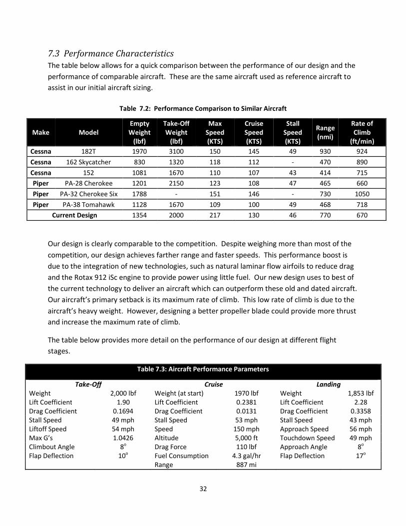
7.3 Performance Characteristics The table below allows for a quick comparison between the performance of our design and the performance of comparable aircraft. These are the same aircraft used as reference aircraft to assist in our initial aircraft sizing.

Make Model Empty Weight

(lbf)

Take-Off Weight

(lbf)

Max Speed (KTS)

Cruise Speed (KTS)

Stall Speed (KTS)

Range (nmi)

Rate of Climb

(ft/min) Cessna 182T 1970 3100 150 145 49 930 924

Cessna 162 Skycatcher 830 1320 118 112 - 470 890

Cessna 152 1081 1670 110 107 43 414 715

Piper PA-28 Cherokee 1201 2150 123 108 47 465 660

Piper PA-32 Cherokee Six 1788 - 151 146 - 730 1050

Piper PA-38 Tomahawk 1128 1670 109 100 49 468 718

Current Design 1354 2000 217 130 46 770 670

Our design is clearly comparable to the competition. Despite weighing more than most of the competition, our design achieves farther range and faster speeds. This performance boost is due to the integration of new technologies, such as natural laminar flow airfoils to reduce drag and the Rotax 912 iSc engine to provide power using little fuel. Our new design uses to best of the current technology to deliver an aircraft which can outperform these old and dated aircraft. Our aircraft’s primary setback is its maximum rate of climb. This low rate of climb is due to the aircraft’s heavy weight. However, designing a better propeller blade could provide more thrust and increase the maximum rate of climb.

The table below provides more detail on the performance of our design at different flight stages.

Table 7.3: Aircraft Performance Parameters

Take-Off Cruise Landing Weight 2,000 lbf Weight (at start) 1970 lbf Weight 1,853 lbf Lift Coefficient 1.90 Lift Coefficient 0.2381 Lift Coefficient 2.28 Drag Coefficient 0.1694 Drag Coefficient 0.0131 Drag Coefficient 0.3358 Stall Speed 49 mph Stall Speed 53 mph Stall Speed 43 mph Liftoff Speed 54 mph Speed 150 mph Approach Speed 56 mph Max G’s 1.0426 Altitude 5,000 ft Touchdown Speed 49 mph Climbout Angle 8o Drag Force 110 lbf Approach Angle 8o

Flap Deflection 10o Fuel Consumption 4.3 gal/hr Flap Deflection 17o

Range 887 mi

Table 7.2: Performance Comparison to Similar Aircraft

33

The tables below provide details of our design’s performance at takeoff and landing. These tables demonstrate that the design can safely take off and land on both a hard, dry runway and on a soft or wet runway.

Soft Surface Hard Surface Ground Roll 354 287 Rotation Distance 159 159 Transition Distance 642 641 Climbout Distance 36 36 Takeoff Distance 1,191 1,125

Soft Surface Hard Surface Air Distance 292 292 Free Roll Distance 145 145 Braking Distance 499 470 Landing Distance 935 907

The figure below provides the drag for our aircraft versus flight speed at cruise altitude. The lift-induced drag was plotted according to the equation for the induced lift coefficient: equation (7.2). The parasitic drag was assumed to increase linearly with airspeed. The figure shows that our maximum speed will occur at around 250 mph, where the drag force meets the total available power. The plot of required power versus available power confirms this maximum speed.

Table 7.4: Takeoff Performance (All distances in ft)

Table 7.5: Landing Performance (All distances in ft)

34

50 100 150 200 250 3000

50

100

150

200

250

300

350

400

Speed (mph)

Forc

e (lb

f)

Drag versus Airspeed

Lift Induced DragParasitic DragTotal DragMaximum AirspeedThrust Available

50 100 150 200 250 30020

40

60

80

100

120

140

Speed (mph)

Pow

er (H

orse

Pow

er)

Power RequiredPower AvailableMax Speed

Figure 7.1: Drag Force versus Airspeed (5kft Altitude)

Figure 7.2: Power Required vs Power Available (5kft Altitude)

35

0 2 4 6 8 10 12 14 16-300

-200

-100

0

100

200

300

400

500

600

700Rate of Climb vs Alititude

Altitude (kft)

Rat

e of

Clim

b (ft

/s)

The figure below shows the rate of climb versus altitude. This plot assumes the aircraft remains at the cruise speed and is at the maximum takeoff weight. At sea level, our aircraft reaches its maximum rate of climb of 670 ft/min. The aircraft’s service ceiling is at 12 kft, where the rate of climb drops below 100 ft/min. This design barely meets the 12 kft minimum service ceiling requirement due to the aircraft’s heavy weight. Flying at a lower weight and/or equipping a more powerful propeller will increase the aircraft’s rate of climb performance.

Figure 7.2: Aircraft Performance at Cruise Speed Versus Altitude

36

8.0 Systems

8.1 Cockpit Sizing In accordance with the Request For Proposal, our aircraft’s cockpit can accommodate pilots of heights anywhere from five to six and half feet. The cockpit is fifty inches in width, which allows for reasonable but non-excessive elbow room, and spans fifty six inches from floor to ceiling to accommodate for pilots up to six and half feet tall, provided that the seat is fully reclined. The relevant dimensions are shown below.

Figure 8.1 Cockpit Layout and Dimensions

Based on the measurements of several group members and volunteers, we determined that the average eye level for pilots of heights from five to six and a half feet is approximately thirty two inches. This allows for an ample view over the control console and nose of the aircraft. The distance between the ceiling and the top of the head for the average pilot will be about six inches. The seat has minimum and maximum reclining angles of five and fifteen degrees from vertical, respectively. There is a small storage space behind the seat, although it can only be reasonably accessed when the aircraft’s door is open (hence, not in flight). The default positions of the aircraft’s yoke and pedals are also based on average values for pilots of heights in the range covered by the Request For Proposals.

37

8.2 Landing Gear Configuration

8.2.1 Landing Gear Analysis The first consideration in configuring the landing gear was the longitudinal tip-over criterion. We placed the main landing gears such that there is a minimum angle of 15° between the aft most center of gravity (CG) and the landing gear vertical centerline. This provides a safe cushion for center of gravity migration along with preventing the airplane from tipping during maintenance. The maximum static strut loads were then determined using the distances between the center of gravity and the wheel-to-ground contact location. The strut loads were calculated using the following equations:

푃 =푊 푙푙 + 푙 (8.1)

푃 =푊 푙

푛 (푙 + 푙 ) (8.2)

Where P represents the strut load in lbf and ns is the number of wheels on the main landing gear, which in our case is 2. The lengths used in equations (8.1) and (8.2) are defined in Figure 8.2 below.

Figure 8.2: Landing Gear Configuration

38

8.2.2 Design Choices Our aircraft’s landing gear are fixed and arranged in a tricycle configuration. Fixed landing gear reduces manufacturing and maintenance costs, aircraft weight, design complexity, and complexity of the takeoff/landing procedure. However, the fixed landing gear impose a drag penalty, but it is fairly small given their small frontal area and our aircraft’s low operating airspeed. The tricycle configuration is very desirable for our aircraft, as it provides a level fuselage on the ground, ground stability, good steering, and good visibility over the nose. The struts have a symmetric NACA 0025 airfoil for a cross-section in order to reduce drag. As mentioned in the material selection section, the struts are made of steel. The benefit of steel is that it can support the same given load as an aluminum strut using a smaller cross-section, since it has greater strength. In accordance, the struts have a thickness of one mere inch and a chord of four inches. These dimensions were calculated at maximum takeoff weight and allow for a rough landing that causes a force of over double the takeoff weight and a safety factor of nearly two. In accordance with the tipping criteria, the design more than satisfies a fifteen degree angle between the plane’s aft-most center of gravity and a vertical plane above the rear wheels, a fifteen degree angle between the same plane and the tip of the tail, and a five degree angle between the nose wheel and the wing tips (see figure on next page). The following table provides the wheel loads and longitudinal wheel placements relative to the tip of the nose and the aft-most longitudinal center of gravity. The values for the main gear express the individual values for each of the two wheels.

Table 8.1: Strut Loading and Wheel Placement

Relative Load Load Distance from

Average C.G. Location Distance from

Spinner

Nose Gear 0.2 WTO 404 lbf 42 in. forward 66 in. aft Main Gear 0.4 WTO 810 lbf 28 in. aft 131 in. aft

The wheel base for the main gear is six feet. This provides sufficient ground stability for our aircraft. The struts all extend two feet vertically below the bottommost point on the fuselage, giving our aircraft the necessary ground clearance. The main struts are placed 5.42 feet apart on the bottom of the aircraft and the struts have total lengths of approximately twenty eight inches. The loading on the main struts is mostly axial. The nose strut also has a total length of approximately twenty eight inches to account for the fact that it is set slightly higher on the aircraft and is swept forward slightly.

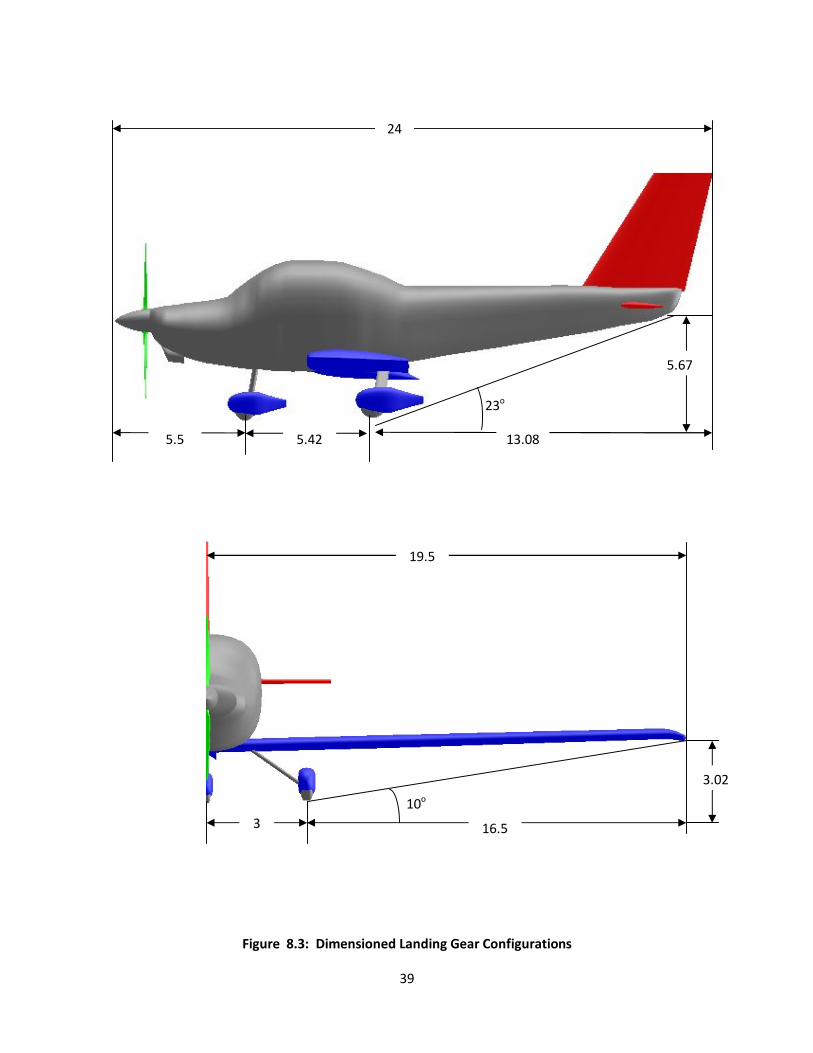
39

5.67

24

23o

13.08 5.42 5.5

10o

3 16.5

3.02

19.5

Figure 8.3: Dimensioned Landing Gear Configurations

40

The wheels use type III low pressure tires. The table below provides the wheel size and tire pressure. These wheels are based on comparable aircraft designs and can comfortably support their given loads without being excessively large.

Table 8.2: Wheel Size and Tire Pressure

Diameter x Width Pressure

Nose Gear 12.5 in. x 5 in. 22 psi

Main Gear 17 in. x 6 in. 19 psi

8.3 Avionics System For the onboard avionics system, we chose to use the Garmin G1000. This system integrates all of the traditional instrumentation of traditional analogue instruments into a large, easy to read glass paneled array. This panel is easy to read and use and will increase the trainee’s awareness of specific flight parameters that he/she must adhere to during training. Since this display system consists of two 10 or 12 inch monitors side by side, there is high visibility of the readouts. The display is customizable and the pilot may choose from flight instrumentation, GPS navigation, weather, terrain maps, traffic conditions, and engine telemetry. With these choices, the trainee may set their screen to flight instrumentation, while the instructor may set their panel to the telemetry to check on the aircraft systems; or set it to the navigation setting to check for the upcoming terrain, location and heading.

Figure 8.4: Garmin G1000 Avionics Display

Another enhanced feature of this display is an autopilot setting which comes built in. This is beneficial because if there is a topic that requires attention of both pilot and trainee, the instructor may switch the aircraft into autopilot, educate the trainee, then easily switch the controls back into manual and continue with the instruction.

41

9.0 Structures and Materials 9.1 Material Selection In the interest of reducing the weight and cost of our aircraft while maintaining its durability, the following materials will be used in its construction. Aluminum 2024, an alloy of mainly aluminum and copper, will be used in the construction of the fuselage and propeller. Aluminum is one of the most common materials used in airplane construction. It is strong in both tension and compression. Although it is not as strong as steel or titanium, aluminum is lighter and cheaper (much cheaper, in the latter case). Furthermore, aluminum also resists corrosion better than steel. Aluminum alloys of the 2XXX series (aluminum-copper alloys) and 7XXX series (aluminum-zinc alloys) are the main aluminum alloys used in airframe construction. Since airframe structures are subject to dynamic loading, our alloy of choice, aluminum 2024, is appropriate for use. It resists fatigue and stress corrosion cracking better than alloys of the 7XXX series, although it has lower ultimate strength and is not recommended for welding. It is worth noting that aluminum is not suitable for use in structures under very high stress or as skin surfaces in supersonic aircraft, which can get very hot due to friction. Since our aircraft is small and limited to subsonic flight, these limitations need not be taken into consideration for the fuselage or propeller. Based on a number of price listings, aluminum 2024 bar stock is approximately three dollars per pound (with a wide tolerance), while aluminum 2024 sheet usually costs about ten dollars per pound. Listed below are the mechanical properties of aluminum 2024.

Table 9.1: Properties of Aluminum 2024 (Ref. 8)

Density 0.1 lb/in3

Ultimate Tensile Strength 68,000 psi

Tensile Yield Strength 47,000 psi

Fatigue Strength 20,000 psi (5x108 cycles

completely reversed stress)

Our aircraft’s lift surfaces will be made out of a composite material, HexTow® AS4 carbon fiber. It consists of carbon filaments in an epoxy matrix. It is lighter and stronger than the other materials used in our airplane. Furthermore, as mentioned earlier, aluminum 2024 should not be welded and would therefore require rivets on the lift surfaces, which would interfere with the airflow and could cause turbulent flow. Use of carbon fiber allows us to do away with the rivets. However, the cost of carbon fiber is somewhat prohibitive, which is why it will not be used for the entirety of the aircraft. Its properties are listed below.

42

Figure 9.1: Wing Spar and Rib Structure

Table 9.2: Properties of AS4 carbon fiber (Ref. 9)

Density 0.0647 lb/in3

Ultimate Tensile Strength 590,000 psi

Tensile Yield Strength 500,000 psi

The aircraft’s landing struts are high-stress components, so they will be made of AISI 4130 steel, a medium carbon steel alloy of chromium and molybdenum. Since the struts are fairly small, the increased density of steel, as opposed to aluminum, will not add a significant amount of weight to the aircraft. Several catalogs list steel bar stock from ten to fifteen dollars per pound. A list of its properties can be found below.

Table 9.3: Properties of AISI 4130N steel (Ref. 10)

Density 0.284 lb/in3

Ultimate Tensile Strength 97,200 psi

Tensile Yield Strength 63,100 psi

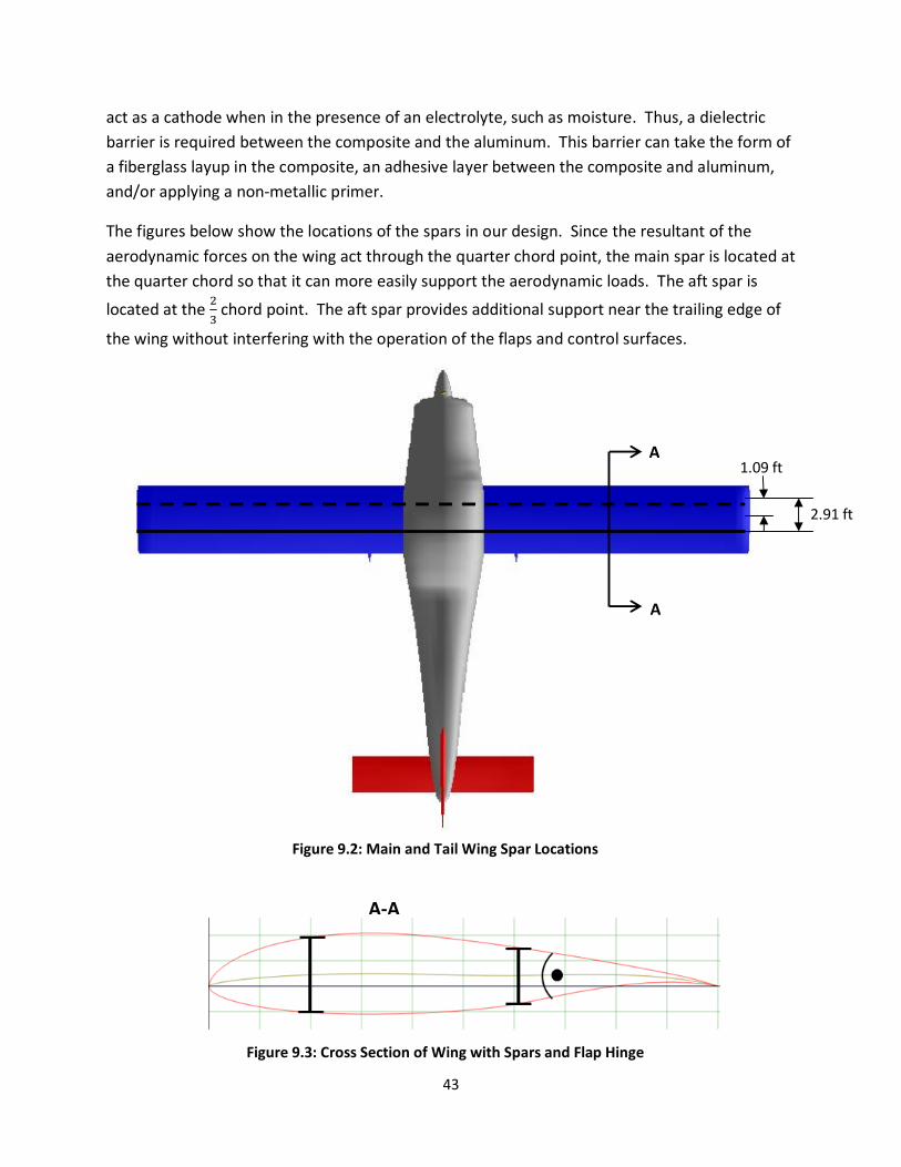
9.2 Structural Analysis The structure of our design’s wings will follow the standard rib and spar design shown below. This design minimizes weight while maintaining sufficient strength to support the aerodynamic loads on the wing. The ribs take the shape of the wing’s airfoil and are spaced along the span of

each wing. The wing box of the rib carries the torsional load on the wing. The holes in the center of the ribs remove weight, while maintaining the strength of the wing box. The main wing is equipped with two spars which run along the span of the wing. These spars support the bending of the wing. The spars and ribs of our design will be constructed of aluminum and the skin of our wing will be constructed of

composite. It is well documented that composites can induce Galvanic corrosion in aluminum, especially in a moist environment (Ref. 18). Although composites are non-corrosive, they can

43

Figure 9.2: Main and Tail Wing Spar Locations

Figure 9.3: Cross Section of Wing with Spars and Flap Hinge

act as a cathode when in the presence of an electrolyte, such as moisture. Thus, a dielectric barrier is required between the composite and the aluminum. This barrier can take the form of a fiberglass layup in the composite, an adhesive layer between the composite and aluminum, and/or applying a non-metallic primer.

The figures below show the locations of the spars in our design. Since the resultant of the aerodynamic forces on the wing act through the quarter chord point, the main spar is located at the quarter chord so that it can more easily support the aerodynamic loads. The aft spar is

located at the chord point. The aft spar provides additional support near the trailing edge of

the wing without interfering with the operation of the flaps and control surfaces.

2.91 ft

1.09 ft A

A

A-A

44

10.0 Cost The financial life cycle of an aircraft can be broken down into four different sections, each as important as the last. These four sections are: Research & Development/Testing, Acquisition, Operations & Maintenance, and Disposal. Each of these segments creates a vital piece of information that we may add up to get an idea for the total cost of the production project, and likewise the price per unit of the final product. In our Request Criterion given in the RFP, two separate production runs will be considered: one run of 500 units and another of 1,500 units produced. Each case will yield a different price per unit, since there are 1,000 more aircraft built in one case than the other, but the prices will not scale exactly due to the overhead costs of each production run being similar. This means that no matter how many aircraft are physically produced, a certain amount of work needs to be done regardless, for example, the Research & Development.

The research and Development is the period during which the design engineers formulate their ideas into a comprehensive aircraft design. This is the time period that we have been working on as a design team. This is the period in which an aircraft is fully designed, then analyzed under various disciplines, only to be re-iterated and tested again. This portion of the aircraft’s development does not entail any physical purchasing of the materials or manufacturing and accounts for roughly fifteen percent of the total cost of the production run.

The next phase for the aircraft’s production is the Acquisition of the materials necessary for fabrication. This is a straight-forward process and entails the purchase of materials necessary for the manufacturing of the plane, along with the fabrication of the aircraft. This is the ‘building’ phase of production and accounts for twenty-five percent of the total cost.

Next is the Operations & Maintenance for the aircraft. This is the longest phase of the aircraft’s life cycle because it is the time period that the aircraft is in actual operation. This cost represents all of the fuel, repair costs, Depot & Overhaul, and Pilot costs for the aircraft. Likewise, this will be the most expensive phase by far, accounting for fifty-five percent of our total design cost.

Lastly, the Disposal cost for our aircraft production must be considered. The Disposal cost is the cost of the airplane at the end of its life cycle, whether that end is recycling or landfill disposal. We have designed our aircraft largely out of aluminum, which will be stripped and recycled. Along with this, we plan to recycle the metallic parts of the electronics systems and mechanical workings of the aircraft. Because of this, we estimate our disposal cost to be ten percent of the total life cycle cost.

45

Table 10.1: Total Lifecycle Cost Breakdown

Table 10.2: Aircraft Cost Comparisons

Phase of production Percentage of Total Cost

R & D 15

Acquisition and Manufacture 20

Operations and Maintenance 55

Disposal 10

With this, we have come up with a life cycle cost of roughly 60 million dollars. This translates to a consumer cost of $150,000 USD per unit. This is a very competitive price upon inspection of the table below, containing the price of competitive aircraft.

Aircraft Cost ($)

Cessna Skycatcher 162 149,900

Cessna Skyhawk 172 289,500

Piper Tomahawk 35,000*

Piper Cherokee 50,000*

* no modern model available on the market, aircraft made before 1980

It can be seen that we offer a design which outperforms its competitors for the same price. With this price per unit, we would generate $75M USD for 500 units and $225M USD for 1,500 units. Thus we estimate to make $15M USD profit for the 500 plane case, and $65M USD for the 1500 plane scenario.

46

11.0 Conclusions and Recommendations Following the methods presented by References 1, 2, and 3 and following the ‘tried and true’ styles of current aircraft design, we set out to design a beginner pilot training aircraft. The goal of our design is to develop an efficient, affordable, and low-maintenance personal air vehicle for use as a trainer aircraft. This design meets or exceeds the requirements set by the RFP. Our design can perform substantially to be able to compete with similar aircraft.

The final configuration is a single engine, propeller-driven aircraft in tractor configuration. The aircraft can carry up two passengers, for a total maximum payload of 450 lbf. The aircraft is equipped with fixed landing gear, has a low wing configuration, and a conventional empennage. The aircraft is very fuel efficient, consuming only 4.3 gal/hr at cruise. This low fuel consumption is due to a combination of an efficient engine and propeller, as well as reduced drag from the wing due to the NLF airfoil. The low fuel consumption allows the aircraft to travel 887 mi on a single tank of fuel. The aircraft is capable of safely taking off and landing on a standard 1,500 ft runway, even in poor runway conditions.

11.1 Recommendations We performed an initial analysis on a possible aircraft design to meet the requirements set by the RFP. Further development and design should be carried out to build upon and finalize the current design presented in this report. Our recommendations for further development are as follows:

Further development should be carried out for the structural integrity of the aircraft. The basic structural layout of the aircraft has been investigated, however, further detail should be analyzed to ensure that the aircraft can support the aerodynamic loads.

Further research should be performed for the life cycle cost of the aircraft. An introductory cost analysis has been performed to estimate a cost for the lifecycle of this design. Further cost analysis should be performed to more accurately determine specific areas of the overall cost of the aircraft. Possible areas for investigation include operations and maintenance, manufacturing and materials, fixed equipment, and finally flight testing of the aircraft.

47

References [1] Roskam, Jan. Airplane Design Part 1: Preliminary Sizing of Airplanes. DAR

Corporation. 2005.

[2] Roskam, Jan. Airplane Desing Part 3: Determination of Stability, Control, and Performance Characteristics, FAR and Military Requirements. DAR Corporation. 2005.

[3] Roskam, Jan. Airplane Design Part 4: Layout Design of Landing Gear and Systems. DAR Corporation. 2005.

[4] Somer, Dan M. 1981. Design and Experimental Results for a Natural-Laminar-Flow Airfoil for General Aviation Applications. NASA Technical Paper 1861

[5] Somers, Dan M. 1981. Design and Experimental Results for a Flapped Natural-Laminar-Flow Airfoil for General Aviation Applications. NASA Technical Paper 1865

[6] McGhee, Robert J., Viken, Jeffrey K., Pfenninger, Werner, Beasley, William D., and Harvey, William D. 1984. Experimental Results for a Flapped Natural-Laminar-Flow Airfoil with High Lift/Drag Ratio. NASA Technical Memorandum 85788.

[7] “Aluminum and its alloys used in aircraft.” NSW HSC online. Board of Studies NSW. 1999. Web. 5 March 2013.

[8] “Aluminum 2024-T4, 2024-T351.” Aerospacemetals.com. ASM Aerospace

Specification Metals, Inc. Web. 5 March 2013. [9] “Product Data.” Hexcel.com. Hexcel. 2010. Web. 10 March 2013.

48

[10] “AISI 4130 Steel, Normalized at 870o C.” Aerospacemetals.com. ASM Aerospace Specification Metals, Inc. Web. 10 March 2013.

[11] Textron Lycoming. O-235 and O-290 Series Aircraft Engines Operator’s Manual. 1988.

[12] Jason. Western Skyways Sales Representitive. (970) 249-0232. March 1, 2013.

[13] Boser, Steve. Sensenich Propeller Sales Representative. steveb@sensenich.com. March 4, 2013.

[14] Nelson, Robert C. Aircraft Stability and Automatic Control. McGraw-Hill, Second Edition, 1998.

[15] Ruijgrok, G.J.J. Elements of Airplane Performance. Delft University Press. 1990.

[16] Woodward, John B. III. Matching Engine and Propeller. June, 1973

<http://deepblue.lib.umich.edu/bitstream/handle/2027.42/91735/Publication_No_142.pdf;jsessionid=D347FC47C7AEB784C521C85A2D4182D8?sequence=1>

[17] G. S. Springer. “Environmental Effect on Epoxy Matrix Composites.” ASTM STP 674. 1978. pp 291-312.

[18] F. Bellucci. “Galvanic Corrosion between Non-Metallic Composites and Metals.” Corrosion, Vol 2

[19] ROTAX Aircraft Engines. Operators Manual for for ROTAX Engine Type 912 i Series. 2012.