Design Optimization with XFdtd EM Simulation Software Using GPU Acceleration and Particle Swarm...
51
© Remcom Inc. All rights reserved. Design Optimization with XFdtd® EM Simulation Software Using GPU Acceleration and Particle Swarm Optimization Broadband Antenna for Use Over Varying Ground Conditions
description
Devices designed for free space operation often fail to meet expectations when deployed in their actual environment. This study considers the example of designing a broadband antenna for an unattended ground sensor using Remcom's XFdtd Release 7 (XF7). To address the challenge of attaining acceptable performance over both dry and wet ground conditions, we use Particle Swarm Optimization (PSO). XStream GPU Acceleration and MPI + GPU technology make this type of sophisticated simulation strategy possible, completing multiple optimizations with hundreds of generations to converge on the best values.
Transcript of Design Optimization with XFdtd EM Simulation Software Using GPU Acceleration and Particle Swarm...

© Remcom Inc. All rights reserved.
Design Optimization with XFdtd® EM Simulation Software Using GPU Acceleration and Particle Swarm Optimization
Broadband Antenna for Use Over Varying Ground Conditions
• Devices designed for free space operation often fail to meet expectations when deployed in their actual environment.
• We will consider the example of designing a broadband antenna for an unattended ground sensor.
• We’ll use several features in Remcom’s XFdtd Release 7 (XF7) to generate and evaluate potential designs: – Particle Swarm Optimization (PSO) – Full wave 3D FDTD solver – XStream® GPU Acceleration
2
Introduction
Unattended Ground Sensor
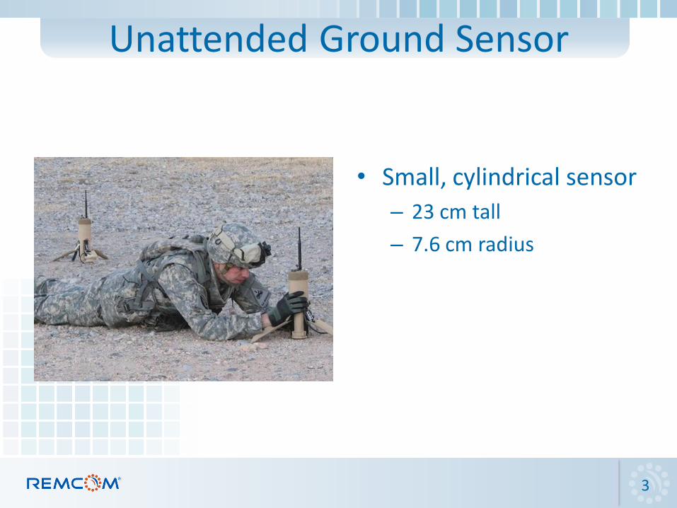
• Small, cylindrical sensor
– 23 cm tall
– 7.6 cm radius
3

• Communicates with other nearby sensors as part of a mesh network
4
Unattended Ground Sensor
• Broadband operation: – 225 MHz - 500 MHz
– Return loss <= -10 dB
• Uniform pattern in the horizontal plane (< 3 dBi variation)
• High gain (>= 5 dBi)
• Near constant gain over bandwidth
• Preference for low-profile solution
• Function over a variety of ground conditions
5
Design Goals

•Repeatedly building prototypes is prohibitively expensive and time consuming.
•The measurement environment includes specific ground conditions that are difficult or impossible to reproduce between measurements.
•This can make it impossible to reliably judge the impact of design modifications.
•Simulation removes this uncertainty from the antenna design process.
6
Benefits of Simulation

• Several broadband antenna choices were considered.
• The broadband sleeve monopole (BBSM) was chosen for performance and size characteristics.
• For the sake of this study, all materials are considered to be perfectly conducting metal.
• Each dimension of the antenna design is defined as a parameter in the software to allow a variety of designs to be simulated.
7
Antenna Choice

Initial Design Lm
on
op
ole
Hsl
eeve
Rtophat
Rmonopole
Rsleeve
Rsleevethick
Parameter Value (cm)
Lmonopole 31.3
Rmonopole 1.0
Hsleeve 13.0
Rsleeve 5.2
Rtophat 2.5
Rbase 7.6
Hbase 15.0
Htophat 0.3
Rsleevethick 0.5
Hb
ase
Rbase
8
• The performance of this antenna design is quite good in free space.
• When the antenna is placed over dry ground the antenna does not operate well over the upper part of the frequency range.
• Over wet ground, the antenna does not operate over most of the range.
Initial Performance
9
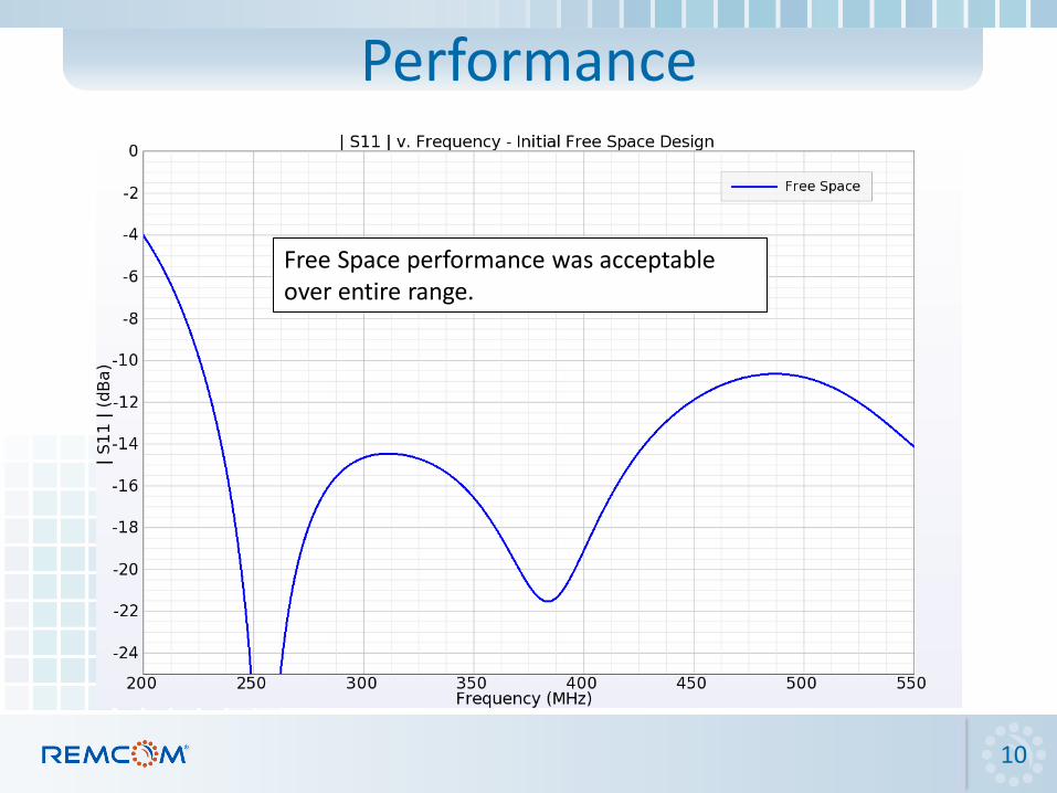
Performance
Free Space performance was acceptable over entire range.
10
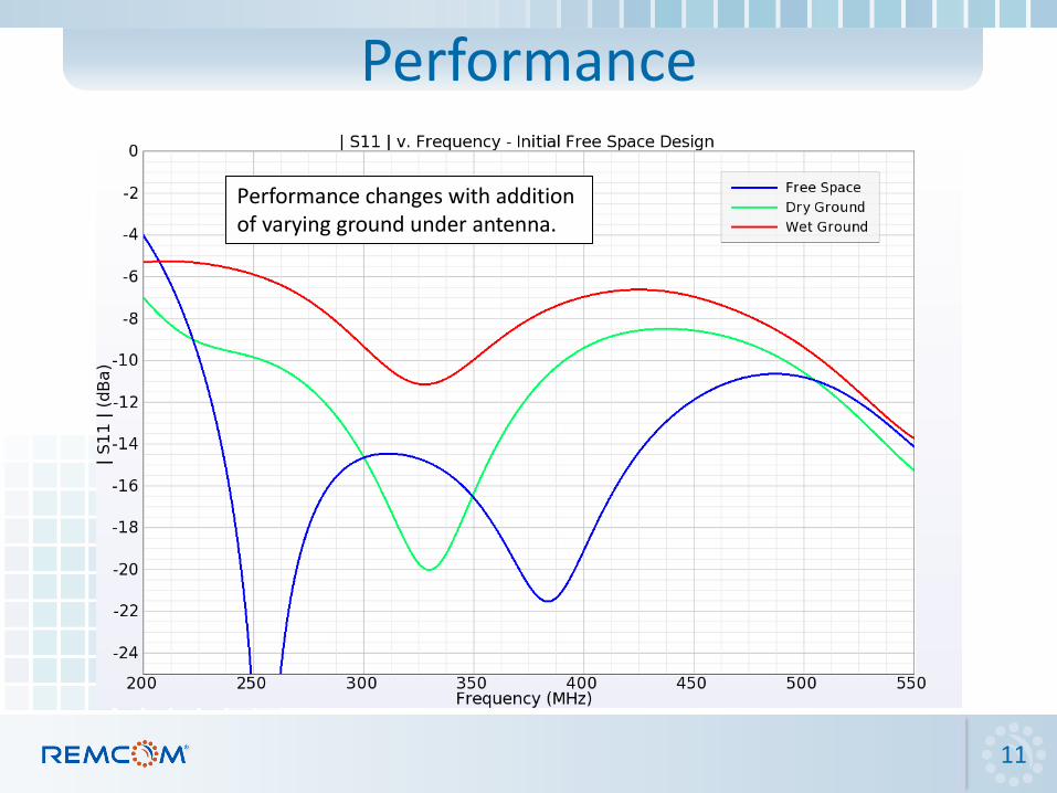
Performance
Performance changes with addition of varying ground under antenna.
11

Performance
Yellow highlights show unacceptable performance regions.
12
• Parameter sweep is impractical.
– We do not know how the parameters interrelate.
• Try a global optimization technique.
– Allows for design by specifying a target goal
– Does not require knowledge of parameter dependencies
– Can be run as a background or asynchronous process
What Now?
13

• Originally presented by Kennedy and Eberhart • Iterative, stochastic optimization technique • Inspired by the social behavior observed in
nature – Flocks of birds – Schools of fish – Swarms of insects
• Each particle represents a potential solution described by its position in the space.
• The suitability of the solution is determined by evaluating a fitness function.
14
Particle Swarm Optimization (PSO)

Particle Swarm Optimization (PSO) • Particles scattered throughout
the solution space • At the start of an iteration,
each particle chooses a new position based on its current position and an updated velocity. • Particle velocity updated as a function of: - Personal best - Global best seen by swarm - Previous velocity
• Process repeated for many iterations (generations)
15
• Particle Swarm Optimization can require hundreds or thousands of iterations to converge on best values.
• Each simulation can take a significant amount of time (minutes to hours), so high performance computing is required.
• Needs are met by using Remcom’s XStream® GPU Acceleration.
16
Computational Needs

• Massively parallelized implementation
• Powered by NVIDIA’s CUDA architecture
• Up to hundreds of times faster than a CPU
17
XStream GPU Acceleration

• For very large problems, one GPU node may not have enough memory.
• MPI + XStream allows a problem to be split among GPUs in multiple systems.
18
MPI + XStream

• Optimizations performed on a loose cluster of machines at Remcom
– Machines physically distributed throughout office
– Each has a variable number of C2050 or C2075 GPUs
– Connected via gigabit Ethernet
– 10 - 12 GPUs available over the course of this work
• Simulations handled by a queuing system which executed each job on a single GPU
– Best approach for maximum throughput
– No communication required between machines
19
PSO Execution

• Use the random nature of the PSO to generate multiple designs.
• This can be achieved by executing multiple independent optimizations.
• Focus on the wet ground environment, because it seems to be the most difficult.
• Investigate the performance of these designs in varying environments.
20
Antenna Design Using PSO
• Focused optimization on five antenna parameters over selected bounds
• Performed five separate optimizations to generate multiple designs
• Chose to use 12 particles in the PSO and permitted each to run up to 200 generations
21
PSO Setup

22
PSO Setup Lm
on
op
ole
Hsl
eeve
Rtophat
Rmonopole
Rsleeve
Parameter Min (cm) Max (cm)
Lmonopole 20.0 40.0
Rmonopole 0.25 1.0
Hsleeve 5.0 19.0
Rsleeve 2.0 7.0
Rtophat 1.0 5.0
• Five Optimizations
– 12 Particles
– 200 Generations

• Unfortunately, no valid design was reached during the initial five optimizations.
• Performed additional five optimizations with 18 particles, each able to reach 600 generations
23
Initial PSO Results

24
Optimization Results
Lmonopole (cm)
Rmonopole (cm) Hsleeve (cm) Rsleeve (cm) Rtophat (cm)
Min Frequency
(MHz)
Max Frequency
(MHz)
26.35 0.3 17.81 2 5 240.3 502.5
26.36 0.3 17.85 2 5 240.3 502.5
26.5 0.3 17.92 2 5 240.3 501.5
26.71 0.3 17.9 2.01 5 240.6 499.7
26.9 0.31 17.84 2.04 5 240.7 500.1
27.96 0.32 18.03 2.12 5 240.8 498.7
26.2 0.3 17.7 2 5 240.8 504.4
26.39 0.3 17.83 2.01 5 240.8 503.0
26.21 0.3 17.87 2.01 4.99 242.0 504.0
38.38 0.35 17.07 2.51 1.05 258.8 488.8
None of the optimizations was able to find an answer that included the lower frequencies of the desired band.

25
Optimization Results
Lmonopole (cm)
Rmonopole (cm) Hsleeve (cm) Rsleeve (cm) Rtophat (cm)
Min Frequency
(MHz)
Max Frequency
(MHz)
26.35 0.3 17.81 2 5 240.3 502.5
26.36 0.3 17.85 2 5 240.3 502.5
26.5 0.3 17.92 2 5 240.3 501.5
26.71 0.3 17.9 2.01 5 240.6 499.7
26.9 0.31 17.84 2.04 5 240.7 500.1
27.96 0.32 18.03 2.12 5 240.8 498.7
26.2 0.3 17.7 2 5 240.8 504.4
26.39 0.3 17.83 2.01 5 240.8 503.0
26.21 0.3 17.87 2.01 4.99 242.0 504.0
38.38 0.35 17.07 2.51 1.05 258.8 488.8
• Optimization Timings: – Generation: 6.8 - 8.2 minutes – Total: 22.8 - 27.4 hours (12 particles, 200 generations) – Up to 120 hours for 18 particles and 600 generations

• PSO did not come up with a valid design despite numerous simulation runs.
• Simulations were very time-consuming, requiring many hours of computer time.
• Essentially no correct result was possible, so the algorithm spent a lot of time trying to fine-tune the best answer it could find.
26
Conclusions of Initial Run
• Try the optimizations again – Run 10 more optimizations
– Look for trends in the parameter values
• Focus on the free space scenario, because it seems to be the least restrictive
• Since we are only looking for trends, we can use a coarser grid to speed up the process – Average time per generation: 2.7 - 3.9 minutes
– Number of generations: 2 - 11
– All ten optimizations completed in 3.25 hours
27
What Next? Understanding Design Tradeoffs
• A sufficient response at the low frequency range in the wet ground scenario was not possible.
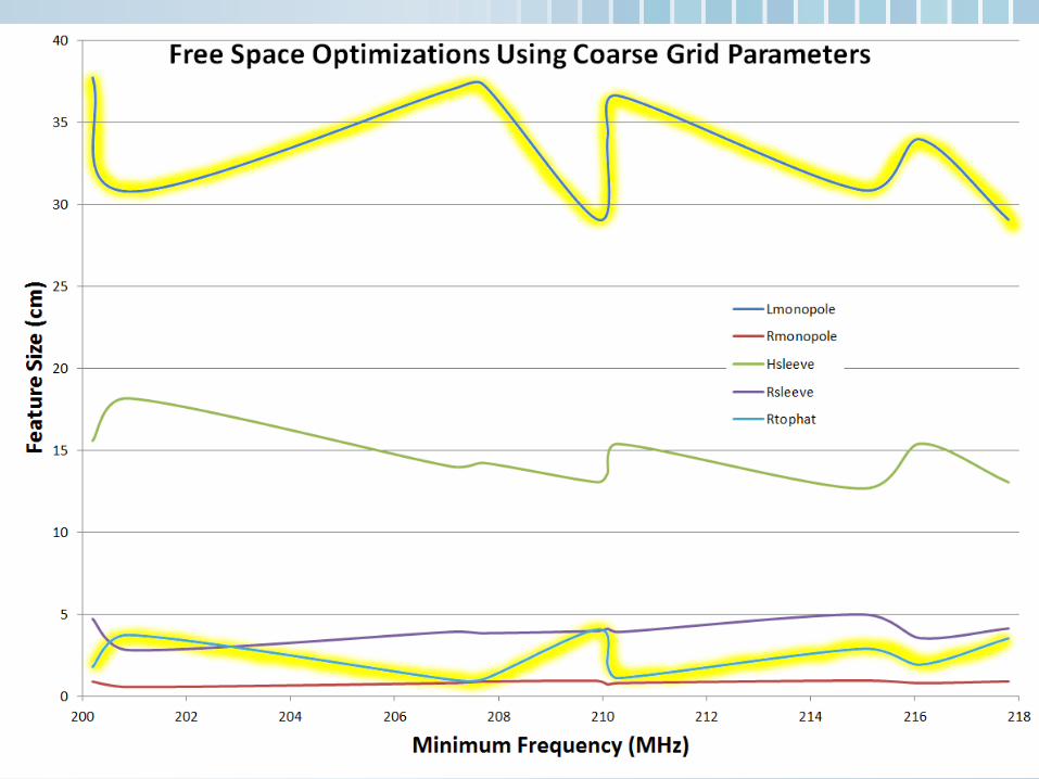
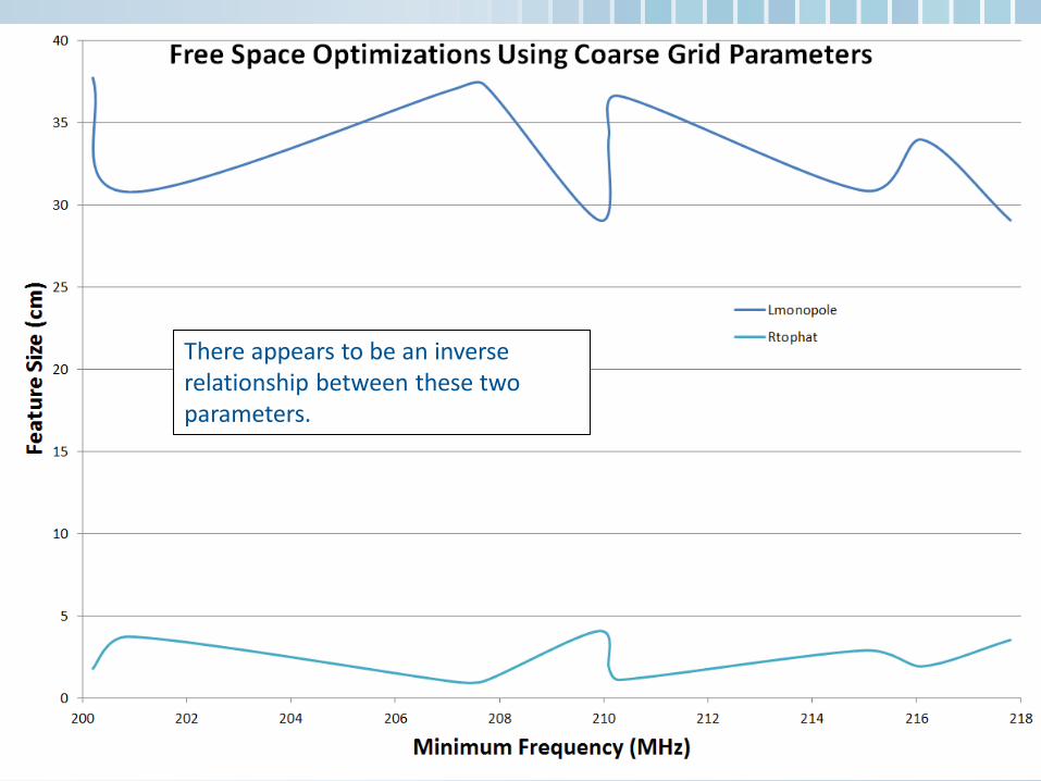
• Generate a plot of parameter values versus minimum achieved frequency to look for trends.
• In the following plots, a relationship emerges between the monopole length and the top hat radius.
28
Observation of Results

29

30
31

32
33
There appears to be an inverse relationship between these two parameters.

34
Some of the best-performing designs were achieved using a small monopole length and a larger top hat radius.

35
Rtophat Maximum
Lmonopole Minimum
A review of the initial restrictions placed on the range of the parameters shows that the maximum radius of the top hat might have been forced to be too small to generate a good design.

• Given this new information, return to the PSO optimization over wet ground and revise the parameter limits.
• Allow for shorter monopole designs by reducing the minimum bound for Lmonopole.
• Allow for larger top hat radii by adjusting the upper bound.
• Adjust the sleeve height to prevent the antenna from shorting out.
36
Revised Optimization
37
PSO Setup Lm
on
op
ole
Hsl
eeve
Rtophat
Rmonopole
Rsleeve
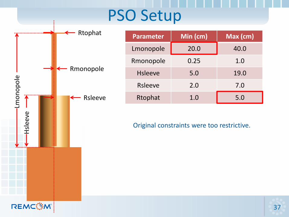
Parameter Min (cm) Max (cm)
Lmonopole 20.0 40.0
Rmonopole 0.25 1.0
Hsleeve 5.0 19.0
Rsleeve 2.0 7.0
Rtophat 1.0 5.0
Original constraints were too restrictive.

38
PSO Setup Lm
on
op
ole
Hsl
eeve
Rtophat
Rmonopole
Rsleeve
Parameter Min (cm) Max (cm)
Lmonopole 5.0 40.0
Rmonopole 0.2 2.0
Hsleeve 2.0 19.0
Rsleeve 2.0 7.0
Rtophat 1.0 8.0
Revised constraints allow for smaller monopoles with larger top hat radii.

39
PSO Setup Lm
on
op
ole
Hsl
eeve
Rtophat
Rmonopole
Rsleeve
Parameter Min (cm) Max (cm)
Lmonopole 5.0 40.0
Rmonopole 0.2 2.0
Hsleeve 2.0 19.0
Rsleeve 2.0 7.0
Rtophat 1.0 8.0
• Re-run with new bounds
• Five Optimizations
– 18 Particles
– 600 Generations
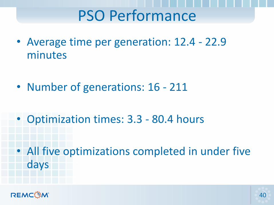
• Average time per generation: 12.4 - 22.9 minutes
• Number of generations: 16 - 211
• Optimization times: 3.3 - 80.4 hours
• All five optimizations completed in under five days
40
PSO Performance

41
Optimization Results
• A variety of acceptable designs were found.
• The second optimization may be best suited to the needs of this project.
Lmonopole (cm)
Rmonopole (cm) Hsleeve (cm) Rsleeve (cm) Rtophat (cm)
Min Frequency
(MHz)
Max Frequency
(MHz)
9.61 1.12 2.47 3.13 7.92 223.4 504.1
20.32 0.5 16.06 2.33 7.96 145.2 545.7
9.65 1.13 2.02 2.9 7.94 220.5 504.7
9.63 1.11 2 2.97 7.87 222.2 503.3
10.48 1.27 2.02 4.01 7.98 212.2 502.9
42
Compare Result to Design Goals
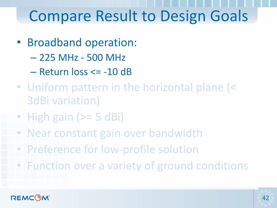
• Broadband operation: – 225 MHz - 500 MHz
– Return loss <= -10 dB
• Uniform pattern in the horizontal plane (< 3dBi variation)
• High gain (>= 5 dBi)
• Near constant gain over bandwidth
• Preference for low-profile solution
• Function over a variety of ground conditions

Both wet ground and dry ground cases meet the goal. Free space does not, but that is not one of the desired operating environments.
43
44
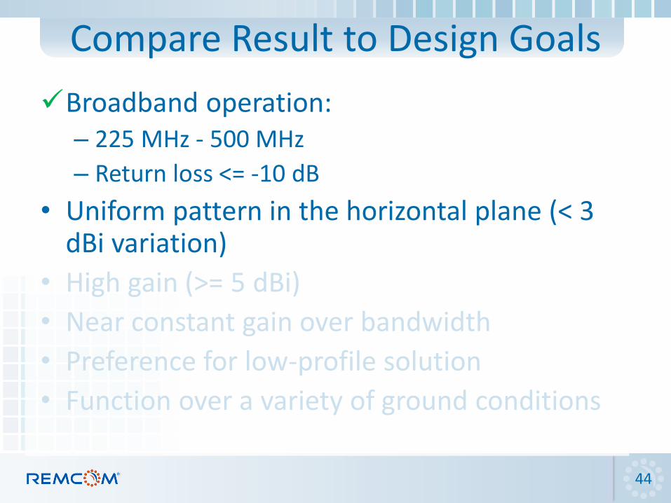
Compare Result to Design Goals
Broadband operation: – 225 MHz - 500 MHz
– Return loss <= -10 dB
• Uniform pattern in the horizontal plane (< 3 dBi variation)
• High gain (>= 5 dBi)
• Near constant gain over bandwidth
• Preference for low-profile solution
• Function over a variety of ground conditions
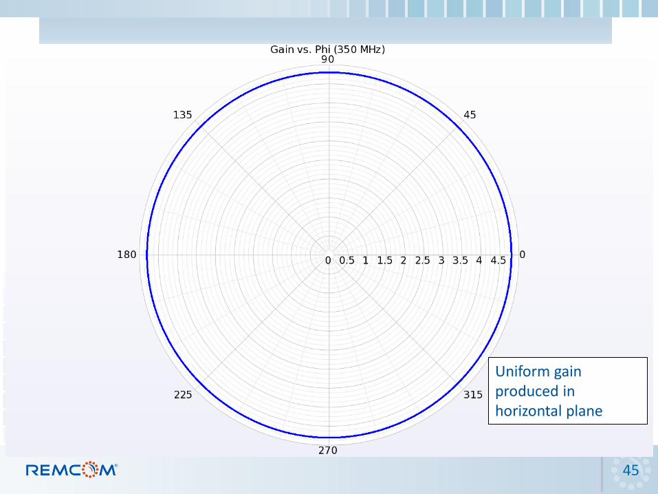
45
Uniform gain produced in horizontal plane
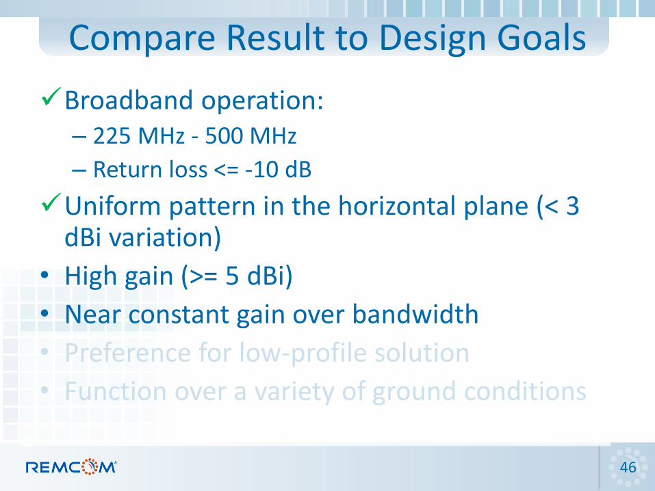
Broadband operation: – 225 MHz - 500 MHz
– Return loss <= -10 dB
Uniform pattern in the horizontal plane (< 3 dBi variation)
• High gain (>= 5 dBi)
• Near constant gain over bandwidth
• Preference for low-profile solution
• Function over a variety of ground conditions
46
Compare Result to Design Goals

Gain is slightly higher than 5 dBi for part of the range with less than 1.5 dBi variation. Not perfect, but acceptable.
47

Broadband operation: - 225 MHz - 500 MHz
- Return loss <= -10 dB
Uniform pattern in the horizontal plane (< 3 dBi variation)
High gain (>= 5 dBi)
Near constant gain over bandwidth
• Preference for low-profile solution
• Function over a variety of ground conditions
48
Compare Result to Design Goals
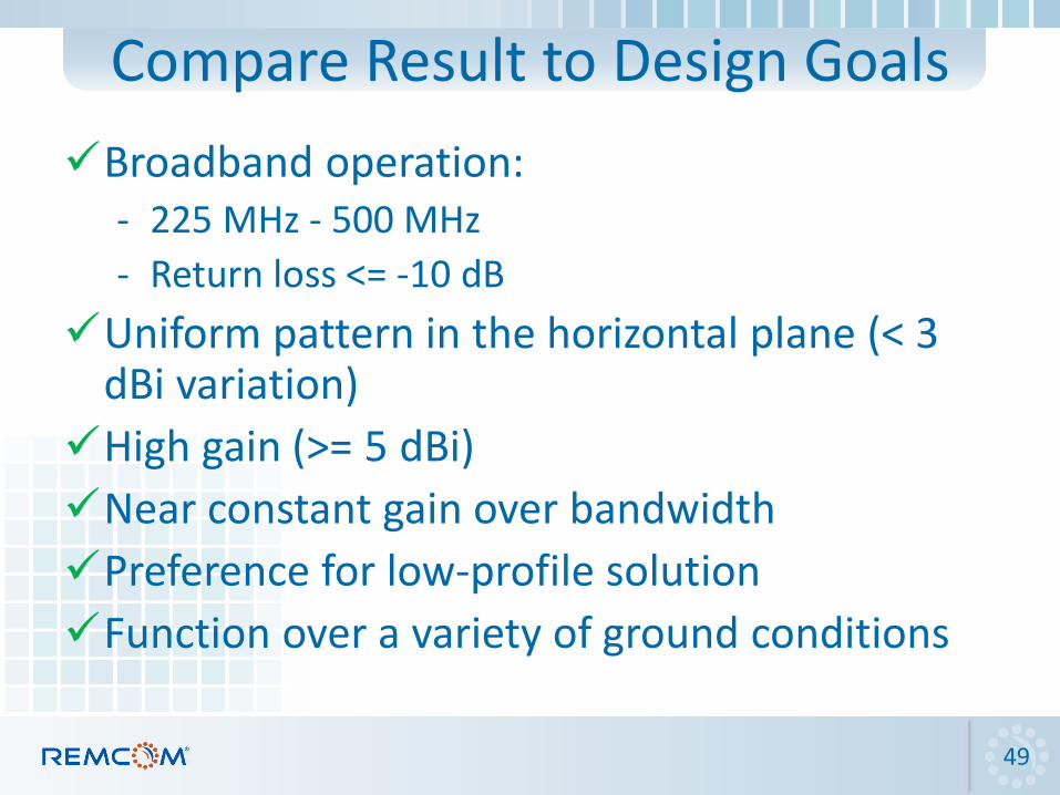
Broadband operation: - 225 MHz - 500 MHz
- Return loss <= -10 dB
Uniform pattern in the horizontal plane (< 3 dBi variation)
High gain (>= 5 dBi)
Near constant gain over bandwidth
Preference for low-profile solution
Function over a variety of ground conditions
49
Compare Result to Design Goals

• When designing an antenna, incorporate as much of the operating environment as possible. – This may limit your choice of simulation tools. – The FDTD method is a robust technique capable of
simulating any environment.
• The random nature of stochastic global optimization techniques can be used to gain insight into complex structures with interdependent parameters. – Use the least restrictive design environment to
generate a variety of solutions. – Employ a coarse grid to speed optimization when
looking for trends.
50
Conclusions

© Remcom Inc. All rights reserved.
Contact us: Toll Free: 1-888-773-6266 (US/Canada) Tel: 1-814-861-1299 Email: [email protected] www.remcom.com Free Trial: www.remcom.com/free-trial-request-form Pricing: www.remcom.com/pricing Information Request: www.remcom.com/information-request-form Google+: https://plus.google.com/+Remcom/posts Facebook: www.facebook.com/remcomsoftware Twitter: twitter.com/remcomsoftware LinkedIn: www.linkedin.com/company/remcom-inc