
Design Optimization of Spillways at Baihetan Hydroelectric Dam946449/FULLTEXT01.pdf · Figure 3....
72
Master of Science Thesis KTH School of Industrial Engineering and Management Energy Technology EGI_2016-049 EKV1148 Division of Heat and Power Technology SE-100 44 STOCKHOLM Design Optimization of Spillways at Baihetan Hydroelectric Dam Oskar Dahl Jack Lönn
Transcript of Design Optimization of Spillways at Baihetan Hydroelectric Dam946449/FULLTEXT01.pdf · Figure 3....

Master of Science Thesis
KTH School of Industrial Engineering and Management
Energy Technology EGI_2016-049 EKV1148
Division of Heat and Power Technology
SE-100 44 STOCKHOLM
Design Optimization of Spillways at
Baihetan Hydroelectric Dam
Oskar Dahl
Jack Lönn

Master of Science Thesis EGI_2016-049
EKV1148
Design Optimization of Spillways at Baihetan
Hydroelectric Dam
Oskar Dahl
Jack Lönn
Approved
2016-06-20
Examiner
Björn Laumert
Supervisor
James Yang
Commissioner
Energiforsk AB & Vattenfall AB
Contact person
James Yang

Abstract
China’s economic prosperity has led to a massive development in the hydropower sector. The Baihetan
hydropower project is an ongoing construction and will become the third largest hydroelectric power
plant in the world in regards to generating capacity and is projected to be finished in the year 2020.
For every fault that an investment this massive has, it will lead to enormous cost and safety risks.
Therefore the standards for every detail are especially high to ensure the success of its future operation.
One of the risks is from the water jet impact on the downstream stilling basin that can cause erosion on
the riverbed. The evaluation of this risk has previously been carried out by an experimental scaled model
at the Department of Hydraulic Engineering at Tsinghua University in Beijing, China. This thesis will
however evaluate the potential of exposing these risks and analyzing methods to minimize them through
Computational Fluid Dynamics analysis.
A Computational Fluid Dynamics model of a surface hole spillway was created in order to be compared
and validated against the experimental results. The results in longitudinal direction are in good agreement
with the experimental results, with an accuracy of the numerical model being 91% for the longitudinal
distance and 98% for the longitudinal spread. The spread in the transverse direction was however
inaccurate with a 40% accuracy in comparison to the experimental results. With a satisfying accuracy in
longitudinal direction and a known error in the transverse direction, the numerical model can be used as
an initial study for optimization by the implementation of a chute block.
After the numerical model was validated against the experimental results, the spillway was redesigned with
a chute block to compare performance compared to the original setup. With the chute block spillway, the
trajectory of the water jet was angled away from the stilling basin’s center, and the longitudinal spread of
the water jet at the impact with the stilling basin increased by 3 m, an increase of 34%. An average
maximum dynamic pressure of 1,9 MPa was located in the center of the bulk flow. With the chute block,
the pressure impact was located 2 m further away from the dam toe.
The results from this thesis shows potential in usage of CFD models in order to evaluate water discharge
performance and that the integration of a chute block shows promise in improving the efficiency of the
spillway. However, the inaccuracies of the numerical model only make it viable to use as an initial study of
design optimization and cannot replace physical scaled models. In order to make final conclusions the
model must be improved further, and with tools of high capacity computational power, the model could
be improved and simulate results closer to reality.

摘要
中国经济的蓬勃发展带来了水电行业飞速的发展。当前正在建设中的白鹤
滩水电站工程就发电容量而言将成为世界第三大水电站。工程预计在 2020
年完成。
对诸如此类的大型投资来说,每一个故障都会导致巨大的经济损失和安全
风险。因此对每个细部环节设立的标准都会尤其的高以保证其在未来正常
的运作。其中一个风险因素来自于水流对下游消力池的冲击作用,这种冲
击会导致河床的冲刷。隶属于清华大学的水利水电工程系利用比例实验模
型已经对上述风险进行了评估。然而,本文将评估分析多种风险因素发生
的可能性,以及从计算流体力学角度分析减少风险的方法。
本文通过建立表孔溢洪道的计算流体力学模型来与试验结果比对。纵向尺
度的结果和试验结果具有很高的一致性,其中数值模型纵向距离和纵向扩
展的精度分别达到 91%和 98%。但横向扩展的结果与试验结果相比只有 40%
的精度。综上所述,纵向尺度的高精度和横向尺度上的小偏差证明这个数
值模型可以被用于初步研究分流墩的实施优化。
在利用数值模型验证试验结果之后,通过对已有的溢洪道重新设计添加一
个分流墩来与原始设计相比,分析其应对性能的变化。陡槽式溢洪道的设
计使得水射流的轨迹偏离消力池,并且水射流由其对消力池的影响使纵向
扩展增加了 3m,增加了 34%。在主体流动的中心存在平均最大值为 1.9MPa
的水压力。因分流墩的存在,压力影响发生在离坝趾 2m远的地方。
本文中的结果体现了 CFD 模型的运用在评估水流流量性能方面的潜力。结
果也显示了分流墩在提高溢洪道效率上的可行性。然而,这个数值模型的
误差性使其只能被用于优化设计的初步研究,并且无法取代物理比例模
型。模型需要被进一步完善以求得到最后的结论,而具有大容量计算能力
的工具的使用使得模型可以被改进从而模拟出更接近实际的结果。

Sammanfattning
Kinas ekonomiska tillväxt har bidragit till en massiv utveckling av vattenkraftsbaserad kraftproduktion.
Det pågående byggnadsprojektet av vattenkraftverket Baihetan planeras att vara klart till år 2020, och när
det står klart kommer det att vara världens tredje största vattenkraftverk vad gäller produktionskapacitet.
För varje felaktighet i en investering av Baihetans storlek, kommer det att uppstå stora ekonomiska
förluster och säkerhetsrisker. Att säkerställa kvaliteten i varje detalj är därför av extra stor vikt för att
undvika förödande konsekvenser. En stor säkerhetsrisk för dammkonstruktionen är erosion av
grundfundamentet nedströms av dammen som resultat av en ineffektiv vattenavledning från utskoven.
Utvärderingar av denna risk har tidigare genomförts genom experiment på en nerskalad modell vid
Institutionen för Hydraulik på Tsinghua Universitet i Peking, Kina. Detta projekt kommer att utvärdera
möjligheten att undersöka detta riskmoment och analysera metoder för att minimera dem med hjälp av en
numerisk CFD-modell.
En CFD-modell för ett av Baihetans utskov har därför konstruerats i syfte att jämföras och valideras mot
data från de experimentella resultaten. Resultaten från den numeriska modellen visar god överstämmelse
med de experimentella resultaten i longitudinal riktning av jetstrålens nedslagspunkt, med en
överenstämmelse på 91% i avståndet från dammen och på 98% i vattnets spridning. Spridningens för
jetstrålens bredd är däremot inte tillräckligt noggrann med en överenstämmelse på endast 40% av de
experimentella resultaten. Med en god noggrannhet i longitudinal riktning och det dokumenterade felet i
transversal riktning, kan CFD-modellen användas för en första analys över effekterna av att optimera
energiavledningen genom integration av ett block i utskovets utlopp.
Efter valideringen av den numeriska modellen optimerades utskovets geometri med ett block vid utloppet,
i syfte att öka spridningen och riktningen för jetstrålen. Det optimerade utskovet testades mot den
originella designen för att utvärdera skillnaderna. Med det tillagda blocket riktades jetstrålen bort från
nedströmsbassängens mitt och den longitudinella spridningen av vattnet vid nedslagspunkten ökade med
3 m, en förbättring på 34%. Ett maximalt dynamiskt tryck på 1,9 MPa för båda utskoven mättes upp i
jetstrålens mitt. Med den optimerade block-designen verkade detta tryck på ett avstånd 2 m längre ifrån
dammen jämfört med den originella designen.
Resultaten visar potential i användningen av CFD-modeller för att utvärdera avledningen av vatten genom
en damms utskov, samt att en integrering av ett block i utskovets utlopp har möjligheten att öka
effektiviteten av energiavledningen. Däremot har den numeriska modellen i sin nuvarande version en
noggrannhet som endast kan användas för förstudier i optimeringsarbete, och den kan inte ersätta fysiska
modeller. För att CFD-modellen ska kunna användas med samma precision som en fysisk modell måste
den utvecklas vidare, och med en ökad beräkningskraft har modellen möjlighet att utvecklas till att nå
verklighetsmässiga resultat.

Acknowledgements
First and foremost we wish to thank Energiforsk AB that funded the project. We also owe a special
thanks to Dr. James Yang from KTH/Vattenfall AB for making this Master´s thesis reality and providing
with all the necessary arrangements.
We would like to thank Huifeng Yu from the Department of Hydraulic Engineering at Tsinghua
University for helping us upon our arrival to Beijing and with our stay Tsinghua campus. He provided us
the right equipment and made sure that the correct software was available on our computers.
We are very appreciative of the guidance given by our supervisors Professor Zhang Yongliang and
Professor Li Ling at the Department of Hydraulic Engineering at Tsinghua University for providing us
with proper guidance throughout the project.
Thanks to our examiner, Associate Professor Björn Laumert at Royal Institute of Technology (KTH) for
reviewing this Master´s thesis and making arrangements at KTH for us.

Table of Contents
1 Introduction .......................................................................................................................................................... 1
2 Aims and Objectives ............................................................................................................................................ 1
3 Background ........................................................................................................................................................... 2
3.1 Chinas Electricity Generation Today ....................................................................................................... 2
3.2 Hydroelectric Development in China ...................................................................................................... 3
3.3 Hydropower Design and Different Types of Dams ............................................................................. 4
3.4 Baihetan Hydroelectric Power Plant ........................................................................................................ 5
3.5 Spillways and Energy Dissipation ............................................................................................................. 5
4 Literature Review ................................................................................................................................................. 8
4.1 Computational Fluid Dynamics Studies .................................................................................................. 8
4.2 Jet Study and Air Entrainment ................................................................................................................10
4.3 Summary of Literature Review ...............................................................................................................10
5 Theory ..................................................................................................................................................................12
5.1 Mesh ............................................................................................................................................................12
5.2 Computational Fluid Dynamics ..............................................................................................................13
6 Methodology .......................................................................................................................................................19
6.1 Hardware and Software Details ..............................................................................................................19
6.2 Geometry ....................................................................................................................................................20
6.3 Mesh Generation and Quality .................................................................................................................25
6.4 Numerical Model ......................................................................................................................................28
7 Results ..................................................................................................................................................................32
7.1 Convergence Analysis ...............................................................................................................................32
7.2 Model Validation .......................................................................................................................................34
7.3 Chute Block Integration ...........................................................................................................................40
8 Discussion and Recommendations .................................................................................................................46
8.1 Numerical Accuracy..................................................................................................................................46
8.2 Spillway Design .........................................................................................................................................46
8.3 Sources of Error ........................................................................................................................................47
8.4 Future Work Recommendations ............................................................................................................48
9 Conclusions .........................................................................................................................................................49
Bibliography .................................................................................................................................................................50
Appendix A Blueprints of Baihetan Hydroelectric Dam spillways ........................................................................ i
Appendix B Results of experimental study using a physical scaled model of the Baihetan dam .................... iii
Appendix C Velocity profiles of the absolute velocity for the Original- and the CB spillway ........................ iv
Appendix D Data set for the Original spillway and the CB spillway simulations .............................................. v

Table of Figures
Figure 1. Electricity energy generation chart (left) (The World Bank, 2016) and installed power capacity
(right) (National Power Planning Research Center, 2013) in China 2012. ........................................................... 2
Figure 2. The dam of Baihetan hydroelectric power plant ..................................................................................... 5
Figure 3. The Kariba Dam and the erosion of its downstream area due to scour from the spillway water jet
discharge. (National Programme on Technology Enhanced Learning, 2015) .................................................... 6
Figure 4. Ogee-crested overflow weir (National Programme on Technology Enhanced Learning, 2015) .... 6
Figure 5. USBR Type III Basin. Stilling basin including chute and baffle blocks to increase the efficiency
of the energy dissipation. (Federal Highway Administration, 1983) ..................................................................... 7
Figure 6. Illustration of structured (TrueGrid, 2015) and unstructured mesh (Pointwise, 2011). ................12
Figure 7. Flow scheme comparison between ITA and NITA (ANSYS Inc., 2006). ......................................18
Figure 8. Workflow of the construction of the numerical simulation. ...............................................................19
Figure 9. Full geometry of the area of Baihetan analyzed. Axes show the distance in meters. ......................20
Figure 10. Geometry of the Original spillway. a) Isometric view b) Top-down view c) Side view ...............21
Figure 11. Boundaries and vertices used for the profile of the ogee-crested weir. Boundaries that are not
specified in the figure are defined as walls. .............................................................................................................22
Figure 12. Geometry of the CB spillway. a) Isometric view b) Top-down view c) Side view ........................23
Figure 13. Dimension of the chute block in the CB spillway...............................................................................23
Figure 14. Boundaries of the downstream area, side view. ...................................................................................24
Figure 15. Boundaries of the downstream area, front view..................................................................................24
Figure 16. Close-up of the downstream mesh. .......................................................................................................25
Figure 17. Mesh of the Original spillway. ................................................................................................................26
Figure 18. Mesh of the CB spillway. .........................................................................................................................27
Figure 19. Residuals for the last 20 iterations/time-steps of the Original spillway simulation. Appendix? .33
Figure 20. Residuals for the last 20 iterations/time-steps of the CB spillway simulation. Appendix? ..........33
Figure 21. Numerical water jet vs. Experimental water jet throw in x-direction. .............................................34
Figure 22. Spread of the water jet at impact height of y=-244 m for the different mesh cases. The color
gradient represents the volume fraction of water between 1% and 100% ........................................................36
Figure 23. Spread range of the water jet at site of impact away from the spillway, x-direction, in relation to
number of meshed cells. .............................................................................................................................................37
Figure 24. Discharge length of the water jet in relation to number of meshed cells. .......................................38
Figure 25. Spread range of the water jet at site of impact away from the spillway, z-direction, in relation to
number of meshed cells. .............................................................................................................................................39
Figure 26. Discharge of the Original spillway .........................................................................................................40
Figure 27. Discharge of the CB spillway..................................................................................................................40
Figure 28. Velocity profile for the outlet of the Original Spillway at different heights. ..................................41
Figure 29. Velocity profile for the outlet of the CB Spillway at different heights. ...........................................41
Figure 30. Comparison of x-velocity between the Original Spillway and the CB Spillway, at a height of y=1
m. ...................................................................................................................................................................................42
Figure 31. Comparison of x-velocity between the Original Spillway and the CB Spillway, at a height of y=1
m. ...................................................................................................................................................................................42
Figure 32. Contour of the water jet spread of the Original spillway, with dashed outline of the spread of
the Chute Block spillway. ...........................................................................................................................................43
Figure 33. Contour of the water jet spread of the CB spillway, with dashed outline of the spread of the
Original spillway. .........................................................................................................................................................43
Figure 34. Dynamic pressure of the water jet from the Original spillway at the stilling basin level y = -244
m. ...................................................................................................................................................................................44
Figure 35. Dynamic pressure of the water jet from the CB spillway at the stilling basin level y=-244 m. ...44

Abbreviations
CFD Computational Fluid Dynamics
VOF Volume of Fluid
ITA Iterative Time Advancement
NITA Non-Iterative Time Advancement
NURBS Non-Uniform Rational B-Spline
Terminology
Spillway The purpose of a spillway is to discharge large amounts of excess water from the
reservoir into the downstream area in a controlled way.
Surface hole A type of spillway that discharges the water from a high height.
Stilling Basin Concrete bedding downstream of the dam to protect the ground from degradation.
Scour Scour occurs when the Stilling Basin´s foundation erodes due to badly controlled
water flow discharge.
Cavitation A phenomenon that evaporates water due to low pressure areas at the spillway. The
water vapor that is created from the low pressure then implodes which results in high
shock forces which can cause wear to the structure.
Chute Block Element added to end of spillway to increase energy dissipation.
Dam A wall structure built to create a reservoir of water and/or to create a height
difference in order to utilize the flow for electricity production.
Cell Is a control-volume created wherein the numerical calculations are made.
Element The cell can have different shapes called element type.
Mesh The numerical geometry is split up into thousands of cells called mesh.
CB Spillway Chute block spillway design.
Original Spillway Original design of spillway without chute block.
Gambit Pre-processing software used to create geometry and mesh.
Fluent CFD-software for the numerical calculation.
TecPlot Post-processing software to visualize the results.

Nomenclature
𝑥 Length
𝑦 Height
𝑧 Width
𝐴 Area
𝐷ℎ Hydraulic diameter
𝑢 Velocity magnitude
�̅� Velocity vector
𝑉 Volume
�̇� Volumetric flow
𝑘 Turbulent kinetic energy
𝐺𝑘 Term for production of turbulence
𝜇𝑡 Turbulent dynamic viscosity
𝜀 Rate of dissipation
𝜎 Prandtl number
𝑝 Pressure
𝜌 Density
𝜃 Angle variable
�̅� Body forces
𝑡 Time
𝜙 Scalar variable
𝑆̅ Surface vector
𝑎 Cell coefficient
𝑏′ Source term for continuity imbalance
𝜉𝑤 Volume of fraction – Water
𝛻 Divergence

-1-
1 Introduction
For a hydropower plant to function safely in every condition, spillways are needed for water to bypass the
dam when the reservoir is becoming full. It is important for these spillways to be carefully designed to
properly dissipate the energy in the water to avoid scour. Poorly designed and constructed spillways can
cause major damage to the foundation of the dam leading to costly reparations and maintenance work, or
in the worst case scenario, a devastating dam failure.
The hydroelectric power projects of the Baihetan dam is one of the largest in the world. The facility needs
to be equipped with proper flood discharge systems that converts the potential energy of the water in the
reservoir in the most convenient way possible. This project aims to investigate the effectiveness of using
CFD in order to predict the outcome of implementing chute blocks on the surface holes in hopes of
successfully dissipate the energy by scattering the jet flow and reducing the impact the water has on the
stilling basin.
2 Aims and Objectives
The aims and objectives of this research is to create a CFD model of a spillway without a chute block to
compare several parameters with real world experimental data. These parameters are the distance the
water jet travels and its spread in both length and width. By this stage, the accuracy of the numerical
model is validated by conducting a mesh independency study to properly decide which quantity of mesh is
optimal in regards to accuracy and computational time required.
The spillway is then re-designed with a chute block and simulated using the same CFD methods as the
previous spillway simulation. The most efficient mesh will be chosen from the findings of the mesh
quality evaluation during the sensitivity analysis. This will increase the credibility of the results in the sense
that similar accuracy can be assumed. The results gained from adding a chute block will then be compared
to the original spillway setup from which conclusions can be made.
In short, the aims and objectives of the research are:
Creation of a CFD-model of the original spillway geometry.
Validation of the CFD-model by comparison to experimental data from a scaled physical model
test performed in an earlier study.
With a validated CFD-model, an optimized design of the original spillway will be analyzed by
adding a chute block to the spillway geometry.

-2-
3 Background
Due to the extreme height of the Baihetan hydroelectric power plant, great caution must be taken into
handling the flood discharge energy dissipation. When discharging large amounts of water through a
surface hole spillway design, the water jet shall preferably dissipate as much energy as possible in order to
reduce the impact of dynamic pressure on the stilling basin. This section will give some background
information of spillway energy dissipation and the Baihetan power plant. An overview of China’s
electricity infrastructure and hydropower development will also be presented.
3.1 Chinas Electricity Generation Today
Fossil fuels are currently dominating China’s electricity generating infrastructure. Coal combustion in
thermal power plants was and still is a cheap alternative to generate electricity. China has massive and
accessible coal reserves and has been an important factor for China’s economic development which in
return has resulted in millions of people leaving the poverty status. As the social perspective has improved
with the economic growth, the environment has been mostly neglected. China is the biggest emitter of
greenhouse gases in the world, responsible for about 28 % of the world’s CO2 emissions from fossil fuels.
(International Energy Agency, 2013)
In 2012, coal had the majority of China’s electricity generation shares at 76% while hydropower had a
share of 17%. Other renewables, nuclear, oil and gas share the remaining 7% of the generation. The
difference between installed capacity and electricity energy output can be seen in Figure 1 below. The
installed power capacity is often misleading for renewable power technologies due to their net capacity
factors being lower. (The World Bank, 2016)
Figure 1. Electricity energy generation chart (left) (The World Bank, 2016) and installed power capacity (right)
(National Power Planning Research Center, 2013) in China 2012.
The current electricity infrastructure in China shows that fossil fuels are dominating, in 2005 the electricity
generation from renewable technologies (excluding hydropower) was close to non-existent. There has
however been several policies implemented since then that has increased the renewable power generation.
In 2013, the installed wind power capacity has grown to 77 GWe and together with other technologies the
total installed renewable power capacity was 380 GWe. The Chinese government set an ambitious target
for renewable power capacity in January 2012 for 2020 so that the total installed capacity for renewable
power sectors is 783 GWe. This will be covered by mostly hydroelectricity followed by wind power,
although solar PV is expected to reach an installed capacity of 100 GWe in 2020. The targets for each
respective technology for 2020 can be seen in Table 1 below. (International Renewable Energy Agency ,
2014)

-3-
Table 1 - Renewable energy targets overview – Targets set by the Chinese government in January 2012 (International Renewable Energy Agency , 2014).
Power Sector 2012 2020
Biomass power 8 𝐺𝑊𝑒 30 𝐺𝑊𝑒
Hydroelectricity 249 𝐺𝑊𝑒 350 𝐺𝑊𝑒
Pumped hydro 20 𝐺𝑊𝑒 70 𝐺𝑊𝑒
Solar PV 5,4 𝐺𝑊𝑒 100 𝐺𝑊𝑒
CSP 0,014 𝐺𝑊𝑒 3 𝐺𝑊𝑒
On-grid wind power 77 𝐺𝑊𝑒* 230 𝐺𝑊𝑒
*From 2013
3.2 Hydroelectric Development in China
China’s first hydroelectric power plant was built in 1912. This was a small facility that had a capacity of
480 kW and is still in operation today (International Hydropower Association, n.d.). The development of
hydropower was slow until the economic boom in the 1980s, when China shifted from a centralized
economy to a market-based. A reform program was created to increase the flexibility of the market,
mostly by reducing the restrictions from the government. This change has led Chinas GDP growth to
average 10 percent per year 1980-2000, which increased the demand for cheap energy. (The World Bank,
2016)
During the early 1980s, China was in dire need of loans to carry out the development of the hydropower
sector. These loans came from foreign governments and corporations such as World Bank and Asia
Development Bank. Also, foreign contractors and engineers with the right competence were imported to
complete hydropower projects. The investments in the hydropower sector led to an increase in capacity
from 20,3 GW in 1980 to 77 GWe in 2000. Hydropower plants have many positive aspects apart from
electricity generation. The ability to control floods, irrigation and water supply are just as important for the
Chinese government. (Xiaofeng, 2013)
From year 2000 until today, the economic growth has averaged around 8 percent per year and is still
increasing its demand for energy. The demand for hydroelectric power plants has increased with the
electricity demand and also the Chinese central government’s incentive to reduce carbon emissions. This
led to an aggressive development during this period, where China’s national hydropower capacity was
increased from 77 GWe in 2000 to 301,8 GWe in 2014 (International hydropower association, 2016).
China has by this period gained skilled engineers which enable manufacturing of hydropower equipment
and components to be produced domestically, making China independent of import. Lastly, China had by
this time acquired an immense amount of capital which made them less dependent of international
financial institutions for the loans needed for the hydropower projects. (Xiaofeng, 2013)
The rapid constructions of hydroelectric power plants were made possible due to governmental
assurances that regulations against hydropower would continue to be close to nonexistent. The
environmental impacts from hydropower were neglected despite the well-known consequences it has.
There is no other electricity generating technology that changes the local environment to the same extent.
The water level is increased upstream and reduced downstream, resulting in massive change in
hydrography. (Xiaofeng, 2013)
China’s potential in hydropower capacity expansion is estimated at 600 GWe, although most probable
exploitability and economics limits this to a more realistic potential capacity of 400 GWe. There are still
many hydropower projects in motion in China (Xiaofeng, 2013). Baihetan Dam is the largest one that is
under construction and will have a capacity of 14 GWe, and is estimated to be completed by 2020 (中国水
利电力对外公司, 2016). The existing and future hydropower plants will continue to be important for
China’s electricity generation.

-4-
3.3 Hydropower Design and Different Types of Dams
A hydroelectric dam is designed by the water flow, the available head and the geographical surroundings
best suited for constructing a dam. The quantity of water flow in a river is however not steady, and the
future flow can be difficult to estimate. Therefore, an extensive hydrological study is carried out at the site
of interest to find data of flow estimates for every day throughout the year. These estimates are taken for
both a wet and a dry year. A flow duration curve is then made that plots the distribution of water flows
for 365 days, from which initial decisions of dam design can be made. (Green For Growth Fund, 2012)
The process of designing the hydroelectric dam is then purely driven by financial motives to insure that
the dam will be as cost-effective as possible. There is a balance between optimum size and design flow for
the dam to be as financially competitive as possible. A rule of thumb is to aim towards satisfying the dam
by setting the optimum design discharge at the 60 day mark in the flow duration chart, meaning the need
for discharge is met or exceeded 16,4 % of the time (Green For Growth Fund, 2012). This optimum will
however vary largely between different projects and is crucial to analyze due to the massive investments
needed to fund the construction. There are three different types of hydropower plants that can be
considered: Impoundment, diversion or pumped storage. (Energy.gov, n.d.)
Impoundment consists of a dam that creates a reservoir of water. These solutions are often implemented on
the biggest hydropower plants in China and are very expensive to build. The river is blocked by the dam
to create a large reservoir of water with as high elevation as possible. (Energy.gov, n.d.)
Diversion is a technique that utilizes a portion of a river through a canal or penstock and is sometimes
called run-of-river. This means that in many instances, it will not be necessary to build a dam to create this
kind of hydroelectric power plant. Utilizing natural elevation height means that diversion is often more
kind to the environment since it does not change the landscape as much as impoundment. These kind of
hydroelectric power plants are therefore reliant on the stream flow at each given moment, since no
reservoir is stored. This can in many cases mean that the facility is unable to generate electricity in the
winter, when demand is highest. (Energy.gov, n.d.)
Pumped storage is a way to increase the water reserve during hours when there is a surplus of electricity in
the grid. In these facilities, the turbine can also work as a pump to convert electric energy to potential
energy in the form of water stored in a reservoir at high elevation. This technology increases the potential
for hydroelectric power plants to adapt to the electric grid and fulfills its role great along renewable energy
technologies, where production hours are fluctuating. The problem with this technology is of economic
nature. The basic idea is to pump water during hours when the electricity price is cheap and generate
electricity during hours when the price is higher. The margin for profitable returns is significantly reduced
when the average price of electricity is low. Conventional electricity generation technologies are improving
their way to vary their output and will therefore be better at adapting to the demand. Although in the
future, with an electricity grid with more renewable power sources, pumped storage might be a great way
to is the most common technology to store large amounts of energy and its usage might be more
impactful in combination with renewable power generation. (Energy Storage Association, n.d.)
In regards to sizes of hydropower plants, they can vary greatly, from a couple of kilowatts to tens of
gigawatts. Hydropower plants with a capacity below 10 MWe are usually defined as small, 10-50 MWe as
medium-sized and bigger than 50 MWe as large. (Energy.gov, n.d.)

-5-
3.4 Baihetan Hydroelectric Power Plant
The largest project in China’s ongoing campaign of expanding their hydroelectric power capacity, is the
Baihetan power plant. With a height of 277 m, a dam crest elevation of 827 m, a crest width of 13 m and a
maximum bottom width of 72 m, the dam can withhold a reservoir capacity of 17,9 billion m3. The
immense energy provided by the Jinsha river and the reservoir capacity of the Baihetan dam, will allow the
power house to utilize 16 generating units to yield an electric power capacity of 14 GWe, with an average
annual energy output of 60,2 TWhe. In addition to the electricity generation of the plant, the construction
of Baihetan dam will give the benefits of increased flood control, silt and soil protection and navigational
improvements (中国水利电力对外公司, 2016). Figure 2 shows a rendition of the dam of the Baihetan
hydroelectric power plant.
Figure 2. The dam of Baihetan hydroelectric power plant
The Baihetan hydroelectric power plant is located in the lower Jinsha River on the borders between the
Sichuan Province and the Yunnan Province, and is the second step in the cascade of a four hydroelectric
dams currently being built in the region. The three dams accompanying Baihetan is Xiluodu, Wudonge
and Xiangjiaba, all with a capacity in the regions of 10 MWe. In combination, the four hydroelectric dams
will have twice the capacity of the Three Gorges hydroelectric plant. Upon completion, Baihetan will be
the tallest dam in China, will have the second largest electrical generation capacity and will be the fourth
largest hydroelectric power plant in the world. (ICA, 2008)
3.5 Spillways and Energy Dissipation
In the cases when excess flood water increases the upstream river height to a level that exceeds the dam
height, the water needs to be released in order to prevent it from overtopping the dam. Passages that
allows excess water to pass the dam are constructed to avoid serious damage to the structure. These
passages are called spillways. For smaller dams, water can be led around the dam structure through
waterways back to the river or to an adjacent river in the area. Larger dams however, store several millions
cubic meters of water and needs to divert the excess water with a more direct and dramatic methods. In
order to not cause erosion in the structure, the spillway of the larger dams need to be robust to withstand
the wear and tear of the large mass flows that ensue. The large mass flows also pose a threat in the area of
impact downstream, where the risk of harmful scour at the bottom of the downstream area is significantly
larger in comparison to within in the spillway structure (National Programme on Technology Enhanced
Learning, 2015). The pressures and velocities involved are hugely destructive, and have caused serious

-6-
problems in large dams earlier. Diversion of excess floodwater through spillways have caused the
foundation of one of Africa’s largest hydroelectric dams, the Kariba dam along the border of Zambia and
Zimbabwe, to reach in a critical state and is in dire need of repairs (Leslie, 2016). Figure 3 below illustrates
the spillway, the water jet, and the erosion present at the Kariba Dam. (National Programme on
Technology Enhanced Learning, 2015)
Figure 3. The Kariba Dam and the erosion of its downstream area due to scour from the spillway water jet discharge. (National Programme on Technology Enhanced Learning, 2015)
The immense volume of water contained by the Baihetan dam requires an effective way to quickly divert
excess water and dissipate the energy in the flow, and sophisticated methods of spillway optimization is
needed. At Baihetan six flood discharge surface holes with ogee-crested overflow weirs will be utilized in
combination with seven mid-level orifices to divert the excess water in a controlled and safe manner, see
Appendix A for details of the spillways at Baihetan.
The Baihetan dam utilize ogee-crested overflow weir spillways to divert excess water. The shape of the
spillways, as shown in Figure 4 below, provides an optimum discharge of the excess water by forming an
ideal form of the lower nappe as the water attaches to the curve of the spillway. This gives a highly
efficient discharge capacity.
Figure 4. Ogee-crested overflow weir (National Programme on Technology Enhanced Learning, 2015)
The profile of the crest is designed from the design head to provide maximum efficiency, stability and
economic feasibility (National Programme on Technology Enhanced Learning, 2015). If the ogee shape
and profile of the spillways is improperly designed, the velocities of the discharge may cause the lower
nappe to detach from the spillway. In this case, air will be entrained beneath the nappe and cause sub-
atmospheric pressures, which can lead to severe cavitation issues. (Chanson, 1995)

-7-
Spillways often include energy dissipators, structural elements that dissipate the energy in the flow before
released to the downstream area. The types of energy dissipators are many, and as with choice of spillway
there is never a generally better method of dissipating the energy for all dams. For each dam type, location
and flow regime, there is a different optimal solution. Common types of energy dissipators all divert the
direction of the flow in order to dissipate the energy. With stilling basins that extends directly after the end
of the spillway with a heel included at the end, a hydraulic jump can be created. The structure creates a
sudden turbulent transition and causes a hydraulic jump, effectively reducing the stress on the downstream
ground. This type of energy dissipators are effective in dams where the toe of the spillway reaches the
water level of the downstream area, as the downstream water depth is required to create the hydraulic
jump.
For spillways located at a certain height above the downstream water level, chute blocks or bucket type
energy dissipators can be included at the end the spillway to increase the energy dissipation of the jet
leaving the spillway. A block or bucket at the end of the sill diverts the direction of the flow, sending the
water in a trajectory away from the dam to a safe distance. Friction forces dissipate the energy both within
the jet and in the interaction between the water jets. The primary gain from an overflow weir type energy
dissipator at a height is not the energy dissipated, but the gained distance of the water jet discharge. This
results in the force of the jet landing at a safe distance away from the dam. One requirement that this type
of solution brings is thus a resilient foundation of the downstream area, and the stilling basin at the site of
impact must either be of solid rock or have a reinforced concrete floor. (National Programme on
Technology Enhanced Learning, 2015)
Figure 5 below shows a schematic layout of a standard USBR Type III Basin (Federal Highway
Administration, 1983). With the addition of chute blocks to the end of the spillway, a more turbulent flow
can be obtained which will aid in the dissipation of energy. The design of the blocks and end sill needs to
be carefully fitted to the specific conditions of the dam in order to achieve maximum efficiency. If the
blocks are used for exceedingly high flow velocities or are improperly designed, there is a high risk of
damage due to cavitation. (Myers, et al., 2015)
Figure 5. USBR Type III Basin. Stilling basin including chute and baffle blocks to increase the efficiency of the energy dissipation. (Federal Highway Administration, 1983)
For the Baihetan hydroelectric power plant, plans are to utilize a combined type of differential flip buckets
and chute blocks for energy dissipation in the spillways of the dam. The addition of buckets and block at
specific locations have the potential to scatter the jet flow and adjust the placement of the discharge, thus
reducing the impact of the dynamic water pressure on the stilling basin effectively. (张永良 & 李玲, 2016)

-8-
4 Literature Review
A study of the literature available on other research regarding CFD-models of spillways and fluid
dynamics has been made. This section has the purpose of presenting the findings that has been used in the
decision-making process of this study, and may provide context for the reader regarding the earlier use of
CFD-models for spillway design.
4.1 Computational Fluid Dynamics Studies
The potential of using CFD-modelling as a complementary tool to physical models have been investigated
in earlier researches. Historically, evaluation of the flow of water over spillways and other fluid dynamic
design problems have been analyzed solely by using physical models. The models are, for large structures,
scaled down versions of the object of study. In literature addressing solutions to design optimization using
scaled models of hydroelectric dams, the scaling ratio is usually 1:40 to 1:50 (Linfield & Mudry, 2008). In
modern times, CFD-models are starting to be involved in the design process, where the CFD model is
supplemented by a physical scale model for calibration of the numerical model and validation of the
obtained results. A physical model provides very precise data on the hydrodynamic events of the discharge
of the spillways where complex physical phenomena of the fluid dynamics, such as air entrainment and
spray, will be correctly accounted for. In a computational simulation, these aspects of the event are often
ignored to save computational power (Gessler & Songheng, 2008). Another limitation of CFD-modelling
is the handling of turbulent flows, a fluid flow phenomena that is very dominant and effects the properties
of the fluid under investigation to a significant extent. It is thus important to model the turbulence as
accurate to the reality as possible. Unfortunately, having the CFD-model solve these complex flow
regimes to a level of accuracy that perfectly resembles reality requires an astounding amount of
computational power. Modeling complex turbulence to absolute certainty is therefore extremely difficult
with the computational power of today. (Sodja, 2007)
A physical scaled model is a popular and reliable method of performing design-tests on a project. It will
account for the complex events of fluid-dynamics such as complicated turbulence regimes, air
entrainment, spray, cavitation, etc., and data that provides an accurate representation of the case of study
can be obtained (Gessler & Songheng, 2008). If necessary, it is possible to analyze design options and
revise the design by altering a portion of the scaled model with minimal resources spent, as opposed to
redesigning the fully scaled object. The experiments and behavior of the case studied can be observed in
real-time when performing test on the scaled model, whereas in a CFD-model, making observations
during the calculated events is difficult. Animating the process is possible in the CFD-model, but the large
computational power needed for the calculations makes animating the process wasteful. Observing the
process and experiencing the effects in real-time can be influential and appreciative for both researchers
and stakeholders of the project. Companies and project stakeholders outsourcing their fluid dynamic
analyses needs to third-party companies, are often more satisfied with the results of a physical model
rather than a CFD-model. (Linfield & Mudry, 2008)
In spite of the benefits of using a physical scaled model in design processes, there are disadvantages and
drawbacks. Designing and constructing the test rig is a costly and time consuming affair, adding the
amount of man-hours and investment costs to the design project. CFD-modelling studies have been
estimated to cost between 20-40% less than performing the study with a physical scaled model, mostly due
to the increased labor intensity and the model construction (Linfield & Mudry, 2008). Other aspects that
influence the cost difference between a physical scaled model and a CFD-model is the increased price of
wind tunnels, which are used in flow analyses, but primarily the decreased cost of high-performance
computers that are necessary for performing an accurate CFD-study. When evaluating high-performance
and high-technology objects, for instance in the aerospace industry, redesigning the physical model for
performance optimization purposes with only minor changes in the geometrical shape, often means that a
new physical model must be constructed. (Swansea University, 2015)

-9-
The measurements and the representation of data obtained from experiments vary between a test using a
physical model and a CFD-model. For a physical model, smoke and strings are used to visualize the flow
inside the fluid compartment of the model. The event is videotaped and analyzed further at a later
processing stage (Linfield & Mudry, 2008). For pressure measurements, there are some difficulties when
using a physical model. The measurement data is obtained by pressure taps placed at specific positions in
the flow. Only a set amount of pressure measurements are thus obtained from the test. As it is not
possible to use an infinite amount of pressure taps, knowledge of where the critical areas of pressure
measurements are located is necessary in order to obtain valuable and useful data from the test
(Groeneveld, et al., 2007). Whereas in a CFD-model, pressure and flow contours can be displayed for
every location in the examined geometry.
What has been proven to be the most successful method of analyzing the design optimization of a
structure dealing with fluid dynamic problems, is to combine the use of a physical scaled model and a
CFD-model. The CFD-model provides a cost-effective and fast tool to initiate the design process, and a
physical scaled model can be constructed at the later stages of the process. The physical model can then
be built from information gathered from the CFD-model, saving resources and time. By combining the
data from experimental tests, a simpler CFD model can be calibrated with the result data acquired from
the scaled model experiments. The CFD model can then accurately model the complex turbulent flows
accurately without the need of a complex solver, and design modifications can be made with an effective
and accurate model. (Gessler & Songheng, 2008)
A study to assess the accuracy of CFD-modelling of spillway hydrodynamic properties in comparison to a
physical scaled model has been made by P. G. Chanel. The commercially available CFD-modelling tool
Flow-3D was used to set up the numerical model in the study. Flow was simulated using the Volume of
Fluid method (VOF) with single fluid flow, and typical properties for water at 20 °C and atmospheric
pressure. Turbulence regimes were calculated with the re-normalization group (RNG) k-epsilon model
with the purpose of maximizing the accuracy of the solution. The result of the study showed satisfying
accuracy between the results obtained from the CFD-model as compared to the results of the physical
model. An analysis of the requirements of mesh refinement was made during the examination of the
numerical model. Using a structured and uniform mesh, it was found that a meshing size of 0,5 m was
sufficient to provide accurate results for the free overflow discharges. Smaller mesh sized were however
required in order to model water surface profiles and quality pressure measurements. For future work, the
study therefore recommends further testing of CFD-models with validation with a physical model in order
to verify the ability of CFD to replicate flow conditions to an accurate level. (Chanel, 2008)
Andersson et. al. investigated the accuracy of estimating spillway capacity with CFD-models in
comparison to a scaled physical model of Höljes dam, located in Klarälven, Sweden. A physical model to
the scale 1:50 was constructed in concrete and sheet metal in order to provide experimental data for the
study. For the CFD-model both a rigid lip approach and the VOF method were tested. Two turbulence
models were tested, a k-epsilon model with scalable wall functions and the Reynold stress model SSG. A
tetrahedral mesh with prism elements was applied to the geometry, and was improved with global
smoothing with regards to the minimum angle and aspect ratio. Four meshes of varying size were used to
examine grid dependency of the model, with sizes ranging from 1,5 million to 8,8 million nodes. In order
to run the computationally demanding calculations of the large mesh size and turbulent flow, a parallel
solver with double precision was used on a 64-bit Linux cluster. From the study it was found that the
results obtained from simulations of the CFD-model were in good agreement with the physical model.
From the results of the different methods used, it was observed that the two turbulence models showed
identical results except in regions of separation, and that the VOF method provided a smoother velocity
profile than the rigid lip approach. (Andersson, et al., 2010)
B. Margeirsson performed a numerical study of the spillways of Vatnsfell hydroelectric dam located in
Iceland. The dam is 30 m high and utilize two spillways, an overflow weir and a bottom outlet, to handle
excess flood water flow. Baffle blocks are placed in the spillway geometry to increase the energy

-10-
dissipation. The discharge capacity, the pressures acting on the structure and the forces on the baffles
where analyzed in FLUENT and compared to experimental results on a physical scaled model. For the
multiphase calculations of the numerical model, the VOF model was used. The study confirmed that a
structured mesh was superior to an unstructured one. Thus, a hexahedral structured mesh of the geometry
was defined at different refinement levels, with the total number of cells ranging from 497 664 to 1 392
594. The study showed satisfying agreement between the results of the numerical simulation and the
physical experiments regarding discharge capacity and pressure acting on the spillway. However, the
numerical results show results that may indicate mesh dependency, and a finer mesh could provide more
accurate results. This would require additional computational power in order to refine the study.
(Margeirsson, 2007)
4.2 Jet Study and Air Entrainment
A previous study in pressure distribution of water jets from flip buckets was carried out by Kerman-Nejad
et al. They found that the maximum pressure of impact occurs at the center of the jet and decreases away
from the center. Reducing the impact angle was also proven to be impactful in order to minimize the
effect that the maximum dynamic pressure has on the stilling basin. In a single water jet, this can be done
by designing the spillway in a way that spreads the water as much as possible. The research emphasizes
that studying the energy dissipation at every stage of a water jet is the key to understanding how scour
formation can be avoided. (Kerman-Nejad, et al., 2011)
If a jet is divided into three different regions, the first region is the free jet, which is the jet when it is in
free fall from the spillway. This region is important to investigate the velocity field and jet thickness.
Experimental results show that the jet widens from the interaction of air, which means that the water is
scattered and mixed with the air. The second region is the impingement region where the jet is being
redirected at impact, here the hydrodynamic pressure from the free jet region is transformed into highly
fluctuating stagnation pressures. It is this transformation that causes the high shear stresses that can cause
damage to the basin foundation as scour formation. The third region is the wall jet region, the water has
by this point been redirected and the flow is aligned with the wall. (Kerman-Nejad, et al., 2011)
The free fall region of the water jet behaves differently depending on several characteristics of the flow. In
laminar flow jets, the bulk flow gets narrower when the velocity increases as can be expected through the
laws of mass continuity. In turbulent jet flows however, the large scale eddies result in a phenomenon
called air entrainment to happen. The water jet is basically gradually mixed with air bubbles through
diffusion and causes the bulk flow to separate. Air entrainment is proven to be significantly higher in areas
of the flow where a lot of turbulence occurs. This phenomenon will then lead to an increase of the cross
sectional area which is preferable since it will spread out the jet. It is proven by research that air
entrainment of as little as 8 % has a significant effect of the reduction on scour. (Chanson, 1995)
4.3 Summary of Literature Review
The literature reviewed suggests that the method of analyzing the design of dam spillways by utilizing a
numerical model validated against experimental results can give satisfying results. The VOF method have
been proven accurate in earlier studies of numerical modelling of spillways, and different models of the k-
epsilon turbulence have been proven to provide results with satisfying resemblance to the results of
experimental studies including a physical scaled model. However, these earlier studies have not analyzed
the flow of a free water jet trajectory through air in a 3D-simulation, and there is not sufficient research on
this specific subject to know for certain that the VOF multiphase model and the k-epsilon turbulence
model can simulate such a scenario with accuracy as well.
The studies by P. G. Chanel, Andersson et al. and B. Margeirsson all show the importance of the quality
and the refinement of the mesh used when analyzing the flow behavior over spillways with CFD-models.
A good quality mesh is of significant importance to provide an accurate solution and is thus a vital part of
the construction of the numerical model. According to the earlier work, a structured mesh will provide

-11-
superior quality to an unstructured mesh. It is also of importance to check the numerical result for mesh
independency, as results that are dependent on the mesh can be very misleading. Refinement of the mesh
is therefore important, where the mesh must at the least be fine enough to provide a mesh-independent
solution, and an even finer mesh will result in a solution of finer accuracy. The smaller sized cells of a
refined mesh will result in an increased total number of cells, which will greatly increase the computational
power needed. In order to obtain a very accurate solution, the demand for powerful hardware therefore
increases. The numerical model can thus not be more accurate than the computational power allows, and
the hardware is thus a constraint that limits the accuracy of the numerical solution. (Chanel, 2008)
(Andersson, et al., 2010) (Margeirsson, 2007)
The studies by Kerman-Nejad et al. found that the maximum pressure from a water jet impact occurs in
the center of the water jet and reduces outwards. Having a smaller impact angle reduces the impact that
the water jet has on the stilling basin. In other words, the water jet should spread out as much as possible
and to have as small of an impact angle as possible. For a water jet to increase its spread and reduce its
hydrodynamic pressure, another study by Chanson acknowledged the significance air entrainment has on a
water jet. It increases the cross sectional area and lowers mean density of the air-water mixed volume flow,
which increases spread and lowers the maximum dynamic pressure. (Kerman-Nejad, et al., 2011)
(Chanson, 1995)

-12-
5 Theory
This section will provide information behind meshing and the methods behind the CFD model. It will
give the reader the chance to understand how these models work and why they were chosen for this flow
simulation.
5.1 Mesh
For a simulation of fluid dynamics to work, the geometry needs to be divided into many small cells. This
method is called meshing and the cells created are where the governing equations can be calculated. The
accuracy of the results gained from the simulation is highly dependent on the mesh size and shape.
Smaller cells will lead to more gradual change in flow characteristics between each cell.
5.1.1 Mesh Structure
The mesh design needs to be adapted to the geometry and type of CFD operation. For 2D applications,
the most common element to be used is usually quadrilateral types and hexahedral elements in 3D (see left
side of Figure 6). These elements are very efficient at covering large areas and work accurate in conditions
where less complexity in geometry and fluid dynamics occur. These kinds of elements are most commonly
used for a structured mesh where the geometry is simple, which greatly reduces computational power
required. For unstructured mesh applications, triangular elements are used to cover more complex
geometry (see right side of Figure 6). In large models, a hybrid mesh could be the smartest solution since
it combines the usage of different elements of both hexahedral and triangular elements. This will reduce
the computational power compared to only using triangular elements while having close to the same
accuracy in critical volumes. (ANSYS Inc., 2007)
Figure 6. Illustration of structured (TrueGrid, 2015) and unstructured mesh (Pointwise, 2011).
5.1.2 Mesh Quality Examination
In order to design an accurate mesh, parameters such as equiangular skewness and aspect ratio is used.
Equiangular skewness is a measurement that determines how close to ideal the shape of a cell is (ANSYS,
Inc., 2009e). It is calculated as
max min,180
e e
e e
Equiangular Skewness max
(1)
where 𝜃𝑚𝑎𝑥 is the largest angle for the cell, 𝜃𝑚𝑖𝑛 the smallest and 𝜃𝑒 the equiangular for the ideal cell (60°
for a triangle and 90° for a square). The closer the value for equiangular skewness is to zero, the better
quality the cell has.
The aspect ratio for a cell is the ratio between the longest edge length and the shortest edge length. The
value of the aspect ratio is defined differently for different element types. The most common elements
(equilateral triangles and hexahedral) have an ideal aspect ratio of one. (ANSYS, Inc., 2009e)

-13-
Mesh smoothness is also an important factor in a mesh. It compares the volume or area of a cell
compared to the adjacent cell. Having mesh transition gradually from smaller to larger cells while keeping
their intended symmetric shape will reduce the risk of numerical error. A well designed mesh will improve
accuracy and also reduce computational power needed for the simulation.
5.1.3 Meshing Scheme
For a volume to be meshed, GAMBIT has different schemes for translating the geometry into logical
shapes into which cells can be created. There are many different methods used to divide geometry in order
to generate the mesh, the methods of relevance to this study are the Submap and the Cooper scheme. The
Submap scheme first divides the geometry into multiple logical cubes and the Cooper scheme divides the
geometry into logical cylinders. The Cooper scheme is necessary for volumes that cannot be divided into
cubes (it is critical that each logical volume has six sides in order for Submap to work). (ANSYS Inc.,
2007)
After a scheme has been chosen for the geometry, the mesh is created and thousands of cells fill up the
entire volume. Submapped models are uniform with hexahedral elements, although for the Cooper
scheme, some wedged elements are created to connect the hexahedral meshes at complex locations (it is
important to check for skewness in these particular areas). (ANSYS Inc., 2007)
5.2 Computational Fluid Dynamics
In this section, the equations and models used in CFD simulations are explained. Emphasis has been
made to describe the terms in the equations to clarify the fluid mechanics that occur. This section will start
by explaining the fundamentals behind the governing equations of CFD and will continue by presenting
information about important models used and considered.
5.2.1 Reynolds-Averaged Navier-Stokes equations
The Reynolds-Averaged Navier-Stokes (RANS) equations describe the motion for flow momentum
transfer and its primary function is to describe turbulent flows. The momentum transfer is defined by two
mechanisms, firstly by the viscosity between fluid layers, called diffusion of momentum. The second
mechanism that creates momentum transfer is the bulk fluid motion between flow regions due to mean
and fluctuating velocity, called advection of momentum. The RANS equations are written as the following
after numerous of derivations from conservation of mass, momentum and energy in order to represent
incompressible flows, (Weisstein, 2005)
2
t
uF p u u u
t
(2)
where �̅� is the body forces on the fluid, 𝜇𝑡 is the turbulent dynamic viscosity and ∇�̅� is the pressure force.
Equation (2) is the finalized form of RANS for incompressible flows and would involve divergence terms
for velocity but is equal to zero for incompressible.
According to the Reynolds number definition, a flow’s characteristics can be described by dividing the
inertial forces with the viscous forces. For incompressible flows with low Reynolds numbers the inertial
term is small and can be seen as insignificant while the viscous term is of influence to the momentum of
the flow. The RANS equation (2) can thereby be rewritten and simplified as the following, (Weisstein,
2005)
2
t
up F u
t
(3)
In the case of higher Reynolds number flows, the viscous forces are small compared to the inertial forces.
The RANS equation (2) can then be reformulated as the following, (Weisstein, 2005)

-14-
u
u u F pt
(4)
The evaluation of the turbulent dynamic viscosity is solved by the usage of turbulence models. There are
different methods provided by FLUENT in order to solve this. The models described in the following
sections are k-epsilon model and Reynolds stress model.
5.2.2 Turbulence Models
There are different models that can be used to handle the turbulence in the simulation. The most
important factor for the model is to account for the turbulence’s impact on the mean flow. The
turbulence appearance and detail are of little interest in most cases but there are more powerful models
able to resemble these factors, although expensive to run. The pros and cons for the most suitable
turbulence model are weighted from their accuracy, simplicity and computational power requirements.
The turbulence models most relevant to this project’s simulation are the k-epsilon and Reynolds Stress
models.
5.2.2.1 Standard k-epsilon turbulence model
The standard k-epsilon model focuses on the mechanisms that has an impact on the turbulent kinetic
energy per unit mass 𝑘 and rate of dissipation, 𝜀. The transport equation as a function of the turbulent
kinetic energy is defined as the following: (Fluent Inc., 2006f)
tk
k
k ku k Gt
. (5)
Equation (5) has been derived from the RANS equations where the effect from buoyancy is neglected,
since it is assumed to be no change in temperature in the jet simulation. The transport equation as a
function of the rate of dissipation 𝜀 is defined as the following: (Fluent Inc., 2006f)
1 2t
ku C G Ct k
. §(6)
Compared to the turbulent kinetic energy equation, which is derived from the exact transport equation,
the rate of dissipation is based from empirical methods and is therefore written in an approximated form.
In the equations above, G𝑘 is the term for the production of turbulence kinetic energy, 𝐶1𝜀 and 𝐶2𝜀 are
model constants, 𝜎𝑘 and 𝜎𝜀 are Prandtl numbers for the turbulent kinetic energy and rate of dissipation
respectively. To solve all unknown variables, a third equation for the turbulent viscosity 𝜇𝑡 as a function
of the turbulent kinetic energy and rate of dissipation is set up as, (Fluent Inc., 2006f)
2
t
kC
(7)
where 𝐶𝜇 is a constant. The default values that are most commonly used for the k-epsilon model are set
as: 𝐶1𝜀 = 1,44, 𝐶2𝜀 = 1,9, 𝐶𝜇 = 0,09, 𝜎𝑘 = 1,0 and 𝜎𝜀 = 1,2. These values are based from experiments
with air and water and have been proven suitable in most applications. The constants enable the k-epsilon
model to function and resemble real-life turbulent shear flow and decay of turbulence. (Fluent Inc., 2006f)
The biggest advantage with k-epsilon turbulence model is its simplicity to use. It offers reasonable
turbulence modeling at low computational power. There is however problems in regards to modelling the
dissipation rate which can lead to result errors, especially for axisymmetric jets. The known weaknesses of
the standard k-epsilon model have led to improvements to enhance the performance. RNG k-epsilon
model and realizable k-epsilon model has led to major improvements and has broadened the application

-15-
availability. For reasons explained below, the realizable model is chosen for the simulation. (Bakker,
2008c)
5.2.2.2 Realizable k-epsilon model
The standard k-epsilon model weakness in modelling the dissipation rate has been improved with
realizable by modifying the transport equation for the dissipation rate. Realizable adjusted the equation for
dissipation rate based on mean-square values for vorticity fluctuations. It is able to take the vorticity
fluctuations into consideration since the model constant 𝐶𝜇 is no longer constant. 𝐶𝜇 is calculated
dynamically as a function of mean strain and rotation rates, while in standard and RNG it is assumed
constant. This adaptation is the most probable reason why studies have shown that realizable performs
better compared to RNG when there are separated flows. (Fluent Inc., 2006c)
5.2.2.3 Reynolds Stress model
The Reynolds Stress Model (RSM) requires the highest amount of computational power of all turbulence
models that Fluent provides. It solves the Reynolds-Averaged Navier-Stokes equations by adding
additional transport equations for Reynolds stresses and one equation for dissipation rate. These extra
Reynolds stresses are also set at the boundary conditions along with the turbulent kinetic energy and
dissipation rate. (Fluent Inc., 2006d)
5.2.3 Multi-Phase − Volume of Fluid
The Volume of Fluid (VOF) model is a setting that calculates the volume fraction for a specific phase, for
instance water volume fraction for water in a volume surrounded by air. With the implementation of
multiple phases, VOF has to take surface tension and wall adhesion into consideration in the momentum
equations. Surface tension occurs when there are attractive forces between molecules in a fluid, only at the
surface of the water volume. This phenomenon creates a resulting force inwards towards the fluid and
increases the pressure. (Bakker, 2008b)
Wall adhesion angle is an option that assumes the contact angle between the fluid and the wall. This
creates a local curvature of the surface near the wall which adjusts the body force term for the surface
tension calculation. (Fluent Inc., 2006g)
Whenever time-accurate transient behavior is wanted from the VOF solution, the geometric
reconstruction interpolation scheme is recommended. It creates an accurate interface between the phases
in every cell and is classified as an explicit formulation of the VOF method (Bakker, 2008b). Explicit
schemes compute the dependent variables directly and are considered more accurate for jet simulations.
(Fluent Inc., 2006a)
5.2.4 Discretization and Gradient Solving Methods
In order to calculate the values of variables (scalars), diffusion terms and velocity derivatives, Fluent uses a
control-volume technique that converts the governing equations to algebraic equations that are solved
numerically, also called discretization. This allows the scalars for the equations to be stored in each
control-volume (cell). The gradient of the scalar 𝜙 at the cell is calculated in Fluent from the Green-Gauss
Theorem, (Fluent Inc., 2006b)
1
1ffc
Faces
SV
(8)
where the gradient (∇𝜙)𝑐1 is the summation of each face’s averaged scalar value �̅�𝑓 times the surface
vector 𝑆�̅� of the face. 𝑉 is the control volume of the element. When the face value is calculated through
the First-Order Upwind scheme, the face value is equal to the cell center average value at the upstream
(opposite direction of the flow velocity) cell. Fluent has an additional setting to improve the face value

-16-
accuracy by either cell or node based gradient solving method. Cell based gradient solving method calculates
the value of the scalar at the face by the arithmetic average of the neighboring cell centers 𝜙𝑐 , (Fluent Inc.,
2006b)
0 1
2
c cf
(9)
Node based gradient solving method on the other hand calculates the arithmetic average of the cell node
values surrounding the node,
1 fN
f n
nfN (10)
where �̅�𝑛 are the nodal values of the surrounding cells. The node based gradient solving method is proven
to be more accurate compared to cell based since it has better capabilities of handling unstructured mesh.
The disadvantage of node based is its higher requirement of computational power. (Fluent Inc., 2006b)
A problem that occurs during a multi-phase simulation with First-Order Upwind scheme enabled is that
the discretization of variables result in an additional false diffusion term called numerical diffusion, which
leads to misleading results. A common method to reduce the numerical diffusion is to use Second-Order
Upwind scheme, which is more accurate because it calculates a higher-order accuracy of the scalars at the
cell faces by using a multidimensional linear reconstruction approach. This results in that the numerical
diffusion is greatly reduced. It is however not possible to use Second-Order Upwind schemes in
combination with explicit VOF methods. This limits the choices of discretization schemes to First-Order
Upwind for these applications. (Fluent Inc., 2006e)
Discretization of pressure can however solved through other interpolation schemes. In many instances,
where the pressure variation between cell centers is smooth, upwind schemes work well. For simulations
where there are large variations between control volume’s pressure gradients, the pressure scalar at the cell
face cannot be interpolated linearly and can lead to divergence of cell velocity. The scheme of interest in
order to calculate the pressure scalar at the cell faces for VOF simulations is the Body-Force-Weighted
scheme. (ANSYS, Inc., 2009b)
Body-Force-Weighted scheme solves the pressure at the cell face by assuming that the normal gradient of the
difference between pressure and body forces are constant. This scheme is valid and accurate in cases
where the body forces are predictable, such as gravity and other centrifugal forces on the fluid. (ANSYS,
Inc., 2009b)
5.2.5 Pressure-Velocity Coupling
Pressure is present in all of the momentum equations and velocity is essential to satisfy the mass
continuity equation. The idea of pressure-velocity coupling algorithms is to derive equations for pressure
from the momentum equations and the continuity equation. The default method in FLUENT to complete
this algorithm is through SIMPLE (Semi-Implicit Method for Pressure-Linked Equations). An equation
for the pressure correction 𝑝′ is derived as the following, (ANSYS, Inc., 2009c)
' ' 'P nb
nb
a p a p b (11)
where 𝑏′ is a source term for the continuity imbalance. Here 𝑎𝑃 is the center coefficient and 𝑎𝑛𝑏 the
influence coefficient for the neighboring cells, which are dependent on the mesh and the flow field.
Equation (11) has a similar appearance as the convection-diffusion equations, partly because SIMPLE is
based on the principle that fluid flows from regions with high pressure to low pressure. (Bakker, 2008a)
There are some improved versions of SIMPLE that significantly eases convergence because they allow
higher relaxation factors compared to SIMPLE. PISO (Pressure Implicit with Splitting of Operators) is

-17-
one of the improved versions and is recommended for transient flow simulations (Bakker, 2008a). It
enables the calculations to remain stable with larger time step and an under-relaxation factor of 1,0 for
momentum and pressure. PISO also has a function called skewness correction that adjusts the pressure-
correction gradient to reduce the error caused from higher angles of skewness. (ANSYS, Inc., 2009c)
5.2.6 Relaxation Factors
After every iteration, the variables of interest are updated within every cell. In order to secure the
simulation’s accuracy, the pressure-based solver uses relaxation factors for the different variables being
calculated. This is in order to adjust the rate of change of these variables to achieve better accuracy.
Although it is favorable to keep the relaxation as high as possible without compromising result accuracy in
order to increase speed of convergence. The new value for a variable 𝜙 is calculated as the following,
(Bakker, 2008a)
, ,new used old new predicted old
P P P PR (12)
where the old value of the variable is added with the difference between the new predicted and the old
value multiplied with the relaxation factor 𝑅. With a relaxation factor less than one (under-relaxation), the
accuracy is increased but the time for convergence is slower. If 𝑅 = 1, the variable will not be affected by
any relaxation factor and the new value will simply be equal to the new predicted value. (Bakker, 2008a)
5.2.7 Residuals and Convergence
Residuals are a measure of error for every equation being calculated in the simulation. Since the magnitude
of value for every variable differs, the residuals are scaled relative to the local value 𝑎𝑃𝜙𝑃 in order to
compare each variable’s error,
P P nb nb
all cells nb
P P
all cells
a a b
Ra
(13)
The scaled residuals 𝑅𝜙 are normalized and will change every iteration. Once the residuals for every
variable have reached a set tolerance, convergence has been reached which means that all cells obey the
conservation equations. The set tolerance is commonly set between 1E-3 to 1E-4. (Bakker, 2008a)
5.2.8 Non-Iterative Time Advancement - NITA
The standard Iterative Time Advancement (ITA) scheme requires a lot of computational power to simulate.
All equations and variables are calculated for every iteration from which the solver chooses to either move
on to the next time step or if the variables are not converged, iterate and calculate all equations again. In
order to reduce the time required for a simulation to finish, the Non-Iterative Time Advancement (NITA)
solution method has been created by FLUENT. The name indicates that there are only inner iterations
within different groups of equations. (ANSYS Inc., 2006d)
A NITA scheme reformulates the Pressure-Based solver algorithms in a way that increases the speed of
the simulation by creating sub-iterations per time step. It is only available with segregated solving method
and it relies on controlling the splitting error that occurs from dividing the solution into sub-iterations.
These sub-iterations mean that different individual set of equations are solved until they converge, only
when converged can the other next set of equations be solved. Once all groups of equations have been
solved, the simulation moves on to the next time step. Since NITA does not solve all equations every
iteration, it is estimated to run about twice as fast as the ITA. The different approaches between ITA and
NITA of solving the different set of equations are illustrated in Figure 7 below. (ANSYS Inc., 2006d)
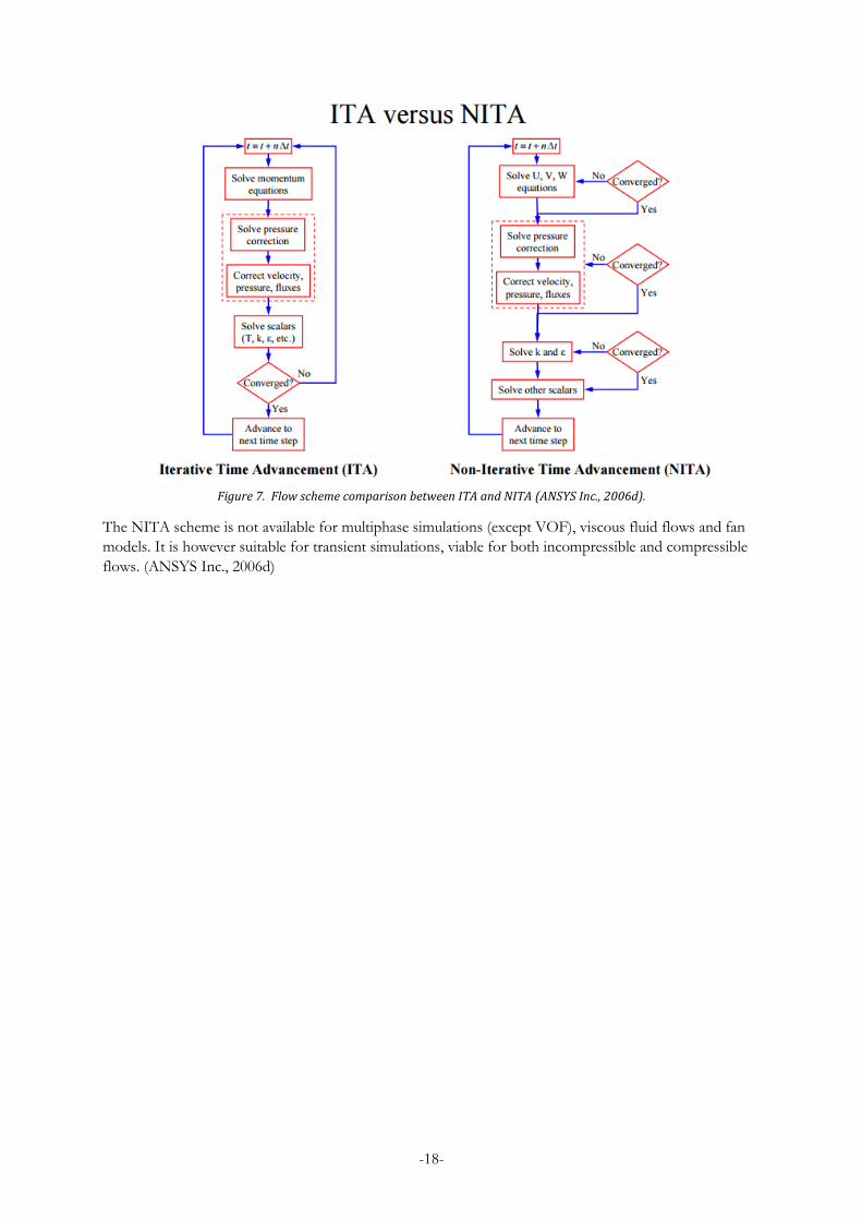
-18-
Figure 7. Flow scheme comparison between ITA and NITA (ANSYS Inc., 2006d).
The NITA scheme is not available for multiphase simulations (except VOF), viscous fluid flows and fan
models. It is however suitable for transient simulations, viable for both incompressible and compressible
flows. (ANSYS Inc., 2006d)

-19-
6 Methodology
The numerical model constructed focuses on spillway number one of Baihetan and the downstream area
of the discharge. Empirical data from experiments performed with a physical scaled model at the
Hydraulic Department of Tsinghua University has been acquired for comparison and validation of the
results of the numerical model. A model with the geometry of the spillway in its original form was
constructed and validated in comparison with the experimental results of the physical model. With a
validated numerical model, an optimized spillway including an energy dissipating chute block called the
CB spillway, was constructed and analyzed. The results of the designs of the original and the CB spillways
were compared versus each other with respect to the velocity profile at the spillway outlet, the discharge
distance and spread and the pressure at impact.
The construction of the simulation was based mainly on three different software programs. GAMBIT
v2.2.30 was utilized for pre-processing and definition of the geometry and mesh, further elaborated in
chapter 6.2 - Geometry. The numerical model was set-up in Fluent v6.2.16 and is detailed in its entirety in
chapter 6.4 - Numerical Model. TecPlot 360 EX 2014 R1 was used for post-processing and the acquisition
of the results. Data used in the graphs, charts and tables in chapter 7 - Results, are attained from TecPlot.
Figure 8 shows the basic workflow of the simulation set-up.
Figure 8. Workflow of the construction of the numerical simulation.
6.1 Hardware and Software Details
The following chapters depicts the details of the hardware and software utilized in the study.
6.1.1 Hardware
Two PC systems with similar hardware were used to separately run simulations. The PCs’ can be regarded
as standard office computers with specifications according to Table 2 below:
Table 2. Hardware used for computation of numerical models
Hardware Computer #1 Computer #2
OS Windows 7, 32-bit Windows 7, 32-bit
Processor Intel® Core™ i7-4770 CPU @ 3.40 GHz Pentium® Dual-core CPU E5700 @ 3.00 GHz
RAM 4 Gb 4 Gb
GPU Intel® HD Graphics 4600 ATI Radeon™ HD 5450
6.1.2 Gambit
Gambit is a pre-processing software developed and sustained by Fluent Inc., which provides a tool to
define geometries and create a mesh with an intuitive user interface. The tool provides the options to
create geometries both by using top-down and bottom-up construction as well as the ability to import
existing CAD models. The meshing tool allows for the geometry to be meshed in sections separately and
with user control, allowing complex geometries to be meshed to the specific demands of the user. An
integrated tool to analyze the mesh quality is provided in the software. (Fluent, Inc., n.d.)
•DefineGeometry
•GenerateMesh
Gambit
•Model set-up
•Numerical calculations
Fluent
•Post-processing
•Result analysis
TecPlot

-20-
6.1.3 Fluent
The commercial CFD-software Fluent was used for construction of the numerical model. Fluent is
utilized by several thousand companies and research facilities around the world. The software has been
tested and proven efficient in several different high-precision industries, ranging from hydroelectric dam
construction companies to formula 1 racing teams using Fluent for their design optimization (ANSYS,
Inc., 2016b). The many capabilities of fluent make the software adaptable to most fluid dynamic scenarios,
and can be utilized for many different cases of flow event. (ANSYS, Inc., 2016a)
6.1.4 TecPlot
TecPlot 360 was used as the post-processing tool used in this study. With the ability to import data from
the numerical model in order to visualize the results, the data can be analyzed in-depth and in careful
detail. Tools for creating line-, 2D- and 3D-plots of important parameters such as velocity and volume
fraction are integrated in TecPlot, and have been used extensively in the process to find key parameters in
the design of the constructed geometry and the numerical model. The data for the end results observed in
chapter 7 - Results are obtained from TecPlot. (TecPlot, 2016)
6.2 Geometry
The section of the Baihetan Hydroelectric dam under investigation is the first spillway of the dam and the
downstream area, which were defined, modeled and meshed. The geometry of the spillway and the depth
of the basin were provided by blueprints of the Baihetan dam, see Appendix A. The downstream area is
constructed from the top of the spillway to the bottom of the stilling basin. In order to model the
downstream area to provide accuracy with a minimum number of meshed cells, the specific geometry was
given by an iterative process where the measurements were adapted to include the water discharge jet
trajectory, and minimize the excessive space to save computational power. Figure 9 below shows the
geometry of the section in its entirety.
Figure 9. Full geometry of the area of Baihetan analyzed. Axes show the distance in meters.
A structured mesh using hexahedral volumes was constructed with the Submap scheme. The constructed
geometry is further detailed for the different sections in chapter 6.2.1, 6.2.2 and 6.2.3. The meshing
process is defined in chapter 6.3 - Mesh Generation and Quality, including details of the mesh quality.
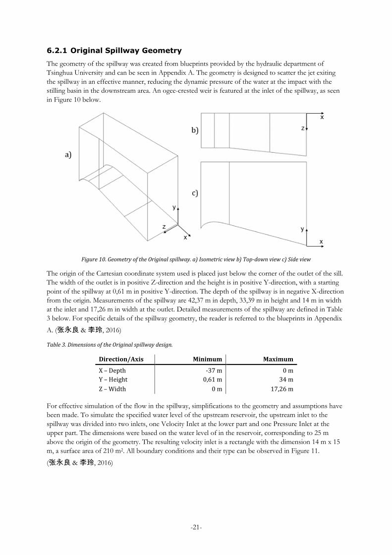
-21-
6.2.1 Original Spillway Geometry
The geometry of the spillway was created from blueprints provided by the hydraulic department of
Tsinghua University and can be seen in Appendix A. The geometry is designed to scatter the jet exiting
the spillway in an effective manner, reducing the dynamic pressure of the water at the impact with the
stilling basin in the downstream area. An ogee-crested weir is featured at the inlet of the spillway, as seen
in Figure 10 below.
Figure 10. Geometry of the Original spillway. a) Isometric view b) Top-down view c) Side view
The origin of the Cartesian coordinate system used is placed just below the corner of the outlet of the sill.
The width of the outlet is in positive Z-direction and the height is in positive Y-direction, with a starting
point of the spillway at 0,61 m in positive Y-direction. The depth of the spillway is in negative X-direction
from the origin. Measurements of the spillway are 42,37 m in depth, 33,39 m in height and 14 m in width
at the inlet and 17,26 m in width at the outlet. Detailed measurements of the spillway are defined in Table
3 below. For specific details of the spillway geometry, the reader is referred to the blueprints in Appendix
A. (张永良 & 李玲, 2016)
Table 3. Dimensions of the Original spillway design.
Direction/Axis Minimum Maximum
X – Depth -37 m 0 m
Y – Height 0,61 m 34 m
Z – Width 0 m 17,26 m
For effective simulation of the flow in the spillway, simplifications to the geometry and assumptions have
been made. To simulate the specified water level of the upstream reservoir, the upstream inlet to the
spillway was divided into two inlets, one Velocity Inlet at the lower part and one Pressure Inlet at the
upper part. The dimensions were based on the water level of in the reservoir, corresponding to 25 m
above the origin of the geometry. The resulting velocity inlet is a rectangle with the dimension 14 m x 15
m, a surface area of 210 m2. All boundary conditions and their type can be observed in Figure 11.
(张永良 & 李玲, 2016)

-22-
Figure 11. Boundaries and vertices used for the profile of the ogee-crested weir. Boundaries that are not specified in the figure are defined as walls.
The ogee-crest overflow weir has the profile of an elliptic curve in the upstream face, given by equation
2 2
2 2
(3,08 )1
5,37 3,08
x y (14)
where 𝑥 is the horizontal distance and 𝑦 is the vertical distance. The curvature of the ogee-crest was
modeled using vertices placed in accordance with equation (14) above and can be observed as gray plus
signs in Figure 11. The vertices were placed at an interval of 0,4 m with an extra fine interval of 0,1 m for
the outermost vertices in the upstream direction. By interpolating between the vertices with a Non-
uniform rational basis spline (NURBS) model, the curvature of the ogee-crest was given and was merged
with the linear slope of the sill.
Downstream of the weirs peak, the elliptic curve continues downwards until it coincides and merges with
the linear slope of the spillway, towards the outlet. The angle of the slope is -15°, and has been designed
to angle the lower jet nappe to the same angle as it exits the spillway outlet. (张永良 & 李玲, 2016)
6.2.2 Chute Block Spillway Geometry
For the CB spillway, one chute block was placed at the end of the sill. The chute block is placed at the
bottom-left corner of the spillways end, as seen from the downstream area facing an upstream direction
towards the spillway. Except for the chute block integrated at the end of the spillway, the geometry is
identical to the geometry of the original spillway. An overview of the geometry of the CB spillway can be
observed in Figure 12 below.

-23-
Figure 12. Geometry of the CB spillway. a) Isometric view b) Top-down view c) Side view
The chute block was constructed from blueprints provided by Tsinghua University, detailed in Appendix
A (张永良 & 李玲, 2016). It features a rectangular face at the outlet of the spillway, measuring 3,60 m in
width and 1,40 m in height. The top of the chute block goes horizontally from the top of the rectangular
face towards the spillway slope, until it coincides with it. This creates a flat and horizontal surface
measuring 5,25 m at the spillway outlet. A detailed view of the geometry and dimensions of the chute
block can be observed in Figure 13 below.
Figure 13. Dimension of the chute block in the CB spillway.
No special modification were needed considering the boundaries of the CB spillway as the basic geometry
is the same and the initial conditions of the simulations will be shared by both the geometries. The
boundaries of the CB Spillway are thus identical to the boundaries of the Original Spillway, as are
displayed in Figure 11 on page 22.

-24-
6.2.3 Downstream Geometry
The downstream geometry has the shape of a simple rectangular box. It was observed that the discharge
jet had the tendency to follow the trajectory of the angled wall of the spillway, pitching the angle of the jet
in the direction of the positive Z-axis. The downstream area was thus given an asymmetrical width. The
height of the downstream area is defined as the height between the top of the spillway and bottom of the
plunge pool, giving a total height of 278 m. Specific details of the downstream geometry can be observed
in Table 4 below.
Table 4. Dimensions of the downstream area.
Direction/Axis Minimum Maximum
X – Depth 0 m 125 m
Y – Height -244 m 34 m
Z – Width -11,5 m 38,76 m
The boundary conditions of the downstream area are set as Pressure Inlet at the top and Wall at the
surface featuring the spillway outlet. The spillway outlet itself is defined as an Interior plane, in order to
give the potential of defining the mesh of the outlet specifically. This way, the downstream area of the
Original and the Chute Block geometries can be kept identical. The sides and the bottom of the
downstream area are defined as Pressure Outlets. This is of extra importance for the bottom surface, as a
Pressure Outlet boundary allows for precision analysis of the water-jet spread at the specific height of
impact. The boundaries of the downstream area can be observed in Figure 14 and Figure 15 below:
Figure 14. Boundaries of the downstream area, side view.
Figure 15. Boundaries of the downstream area, front view.
The shape was chosen to provide enough space to simulate the water jet discharge, while at the same time
allowing the geometry to be meshed with a structured mesh and hexahedral elements. With the simple
geometry giving a high quality mesh, the numerical model is allowed to converge more easily, while giving
accurate results.

-25-
6.3 Mesh Generation and Quality
For generating the mesh of the two geometries, the spillway and the downstream areas were fused. Two
meshes were generated, the Original spillway and the Chute block spillway. Both feature the downstream
area which is identical between the two geometries. In order to provide a mesh with a good cell quality,
the width of the downstream area was constructed to keep an equal aspect ratio with the spillway outlet to
allow a structured mesh to be defined with a quality as high quality as possible. A close-up of the
downstream mesh can be seen in Figure 16.
Figure 16. Close-up of the downstream mesh.
Two factors are deemed as the most important to analyze in order to create a mesh of high quality, the
equiangular skewness and the aspect ratio (ANSYS, Inc., 2009e). The equiangular skewness is the
difference between the shapes of a meshed hexahedral cell in comparison to a perfect hexahedral cell
where all angles are equal. It is recommended not to exceed a skewness value of 0,85, and a value of
skewness in the interval of 0,00 – 0,25 can be considered as excellent quality. (Bakker, 2002)
The aspect ratio, which represents the stretching of a cell, has its optimum at a 1:1 ratio where all sides of
a cell are equal in length. It is recommended to not exceed an aspect ratio of 5:1 in order to construct a
high quality mesh (ANSYS, Inc., 2009e). For details regarding the factors, see chapter 5.1.2 - Mesh Quality
Examination.
6.3.1 Original Spillway Mesh
As the geometry of the Original Spillway is relatively uncomplicated and does not feature complex
elements and details, a structured mesh was used to provide fast and accurate numerical calculations in
accordance with chapter 5.1.1 - Mesh Structure. For the original geometry, hexahedral cells were used to
provide qualitative calculations, rather than tetrahedral or wedge cells. A zoomed in view of the mesh,
only including the spillway and excluding the downstream area, can be observed in Figure 17.

-26-
Figure 17. Mesh of the Original spillway.
The cell with the poorest quality in the constructed mesh has an equiangular skewness of 0,16 and the
large majority of the cells in the mesh, representing 99,03% of the total, are of an equiangular skewness of
0,05 or below. As 100% of the cells are of an equiangular skewness below 0,25, the mesh can be
considered as being of excellent quality. Details of the number of cells in different intervals of equiangular
skewness are presented in Table 5 below.
Table 5. Equiangular skewness for the cells in the constructed mesh of the original geometry.
Equiangular
skewness No. of cells
Percentage
of total cells
>0,16 0 0%
0,10 – 0,16 2 560 0,46%
0,05 – 0,10 2 855 0,51%
0,00 – 0,05 553 965 99,03%
The highest aspect ratio present in the mesh have a value of 1,5:1. The majority of the cells however,
representing 91,03% of the total, have an aspect ratio between 1,1:1 and 1:1. Different intervals of aspects
ratios and the number of cells affiliated with the value are presented in Table 6 below.
Table 6. Aspect ratio for the cells in the constructed mesh of the original geometry.
Aspect Ratio No. of cells
Percentage
of total cells
>1,5:1 0 0%
1,1 :1 – 1,5:1 50 186 8,97%
1:1 – 1:1,1 509 194 91,03%
The values presented in Table 5 and Table 6 indicates a mesh of high quality with values of the important
factors well below the recommended limits.
6.3.2 Chute Block Spillway Mesh
As the chute block integrated in the CB Spillway provides a more complex geometry with sharp angles, a
structured mesh with hexahedral elements is impossible. For the CB Spillway, a hex/wedge mesh was
necessary in the vicinity of the block, meshed with the Cooper scheme. The mesh does however have a
close resemblance to a fully structured mesh, and can be observed in Figure 18.

-27-
Figure 18. Mesh of the CB spillway.
The mesh of the CB Spillway has a majority of the cells, at 99,94% of the total, within the range of 0,00 –
0,25 equiangular skewness. The range in skewness is wider in comparison to the original spillway
geometry, with the poorest quality cell having an equiangular skewness of 0,84. However, as less than
0,01% of the cells have a skewness greater than 0,50, the mesh is considered well suited for simulation.
Details of the meshed cells skewness for the CB geometry can be seen in Table 7 below.
Table 7. Equiangular skewness for the cells in the constructed mesh of the CB geometry
Equiangular
skewness No. of cells
Percentage
of total cells
> 0,85 0 0%
0,50 – 0,85 19 < 0,01%
0,25 – 0,50 282 0,05%
0,00 – 0,25 527 400 99,94%
The aspect ratio of the cells in the CB geometry contains a higher aspect ratio in comparison to the mesh
of the original geometry. Two cells in the mesh exceeds the recommended value of 5:1 by a small amount,
with aspect ratios of 5,55:1 and 5,60:1 respectively. However, the majority of the cells, at 99,99% of the
total, have an aspect ratio between 1:1 and 2:1, which can be considered as high quality cells Table 8
displays the number of cells in different intervals of aspect ratios.
Table 8. Aspect ratio for the cells in the constructed mesh of the CB geometry.
Aspect Ratio No. of cells
Percentage
of total cells
5:1 – 6:1 2 < 0,01%
2:1 – 5:1 48 0,01%
1:1 – 2:1 527 651 99,99%
Despite the fact that the cells in the mesh of the CB geometry are of poorer quality than the cells in the
original geometry, the mesh can still be considered as containing high-quality. As the majority of the cells
in the CB geometry falls in the categories considered as excellent quality or well beyond recommended
limits, the mesh is of a quality with the potential of providing accurate results.

-28-
6.4 Numerical Model
This chapter is dedicated to the configuration of the numerical model utilized in the study. The model was
completely set-up using FLUENT software, the initial and boundary conditions were acquired from real-
world experimental data.
The following sections include the settings for the numerical model set-up in FLUENT. Important
settings are highlighted in bold text, to allow for a comprehensible overview of the model. Settings not
mentioned in the sections below have been left at default values and settings.
6.4.1 Solver
An unsteady solver in 3D Double Precision mode was used for the numerical model. The transient
event of the discharge is of utter importance in the simulated event, thus making a steady solver
counterproductive and impractical. In order to capture the spread of the jet in all directions, a 3D model
was necessary. Double Precision mode was used to capture the flow events of the discharge with the
highest possible accuracy. The NITA scheme was used to reduce the time needed for the numerical
calculations, see chapter 5.2.8 - Non-Iterative Time Advancement - NITA, for details.
A pressure-based solver with an implicit solution approach and segregated solver algorithms and was
utilized for the numerical model. The pressure-based solver offers a robust, accurate and flexible solver
that can be used with a low impact on memory usage. An implicit approach is favored over an explicit in
most cases, cases involving supersonic speeds and shock waves being an exception. The segregated solver
algorithms must be used when simulating multiphase flow using the VOF method, see chapter 5.2.3 -
Multi-Phase − Volume of Fluid. As the simulation scenario of this study does not require special attention
of a density-based solver with an explicit approach, the robust and efficient method of a pressure-based
solver was deemed as the most practical. (ANSYS, Inc., 2006c)
The body-force-weighted scheme was utilized as interpolation scheme for calculating cell-face pressures.
As the simulated scenario is expected to involve predictable and large body forces, the body-force-
weighted scheme was deemed as the most suitable scheme for the numerical model. (ANSYS, Inc., 2009b)
For all interpolation methods except for the pressure interpolation, the First-Order Upwind
interpolation scheme with Green-Gauss Node-Based gradients of solution variables were utilized. The
First-Order Upwind scheme provides an interpolation scheme with a better ability to reach convergence
compares to other schemes. This is however at the expense of accuracy. For better accuracy the
interpolation scheme can be changed to Second-Order Upwind, preferable after convergence has been
met by the First-Order Upwind scheme. The Second-Order Upwind scheme is not used in this study due
to restraints in available computational power and limitations of the VOF-model (ANSYS, Inc., 2006b).
The Green-Gauss Node-Based gradients of solution offers an accurate solution and was chosen to
minimize the potential false diffusion in the solution obtained. The result of the utilization of a Green-
Gauss Node-Based solver is a more defined boundary between the water jet discharge and the
surrounding atmospheric air. (ANSYS, Inc., 2006c)
The Pressure Implicit Splitting of Operators (PISO) approach was used for the pressure-velocity coupling
algorithm of the numerical model. The PISO algorithm is highly recommended as the algorithm to utilize
for transient flows and can be considered reliable and robust. The algorithm is able to handle larger time
step than other alternatives, having the potential of a faster computational time. No parameters or
attributes of the simulated scenario required additional attention that can be provided by other pressure-
velocity coupling algorithms, therefore rendering the other algorithms redundant (ANSYS, Inc., 2009c).
6.4.2 Multiphase Scheme
The explicit Volume of Fluid (VOF) method was used to model the multiphase properties of the
simulation. The method has been proven a simple and efficient technique in scenarios including multiple
phases and free boundaries, and can be used in three-dimensional problems. A particularly practical aspect

-29-
of the VOF method over other multiphase schemes is its ability to numerically treat the multiphase flow
with a minimum amount of stored information, decreasing the computational time and complexity of the
simulation. (Hirt & Nichols, 1981)
The geometric reconstruction scheme has been used for interpolation between cell faces, as it is
considered as the recommended scheme in combination with the explicit VOF-model for simulations of
jet-breakup problems. (ANSYS, Inc., 2009a). As the large body forces of gravity and surface tension are
present in the multiphase flow, the implicit body force treatment has been enables and applied to help
the solution being more robust.
6.4.3 Turbulence Model
The realizable k-epsilon turbulence model was used for the simulation because of its proven
robustness. The improvements from the standard k-epsilon model give it enough accuracy while being
economical in computational power. It can more accurately predict spreading rate, flow rotation,
boundary layers with strong adverse pressure gradients, separation and recirculation. These improvements
satisfy some constraints on the Reynolds stresses, which are important for the physics of turbulent flows.
This is the most probable reason why studies have shown that realizable performs better compared to
RNG when there are separated flows. (Fluent Inc., 2006c)
Studies have shown that the Reynolds Stress Model (RSM) has superior abilities when it comes to simulate
curvature, swirl, rotation and other complex flows. Although for simpler flows, the advantages compared
to the two-equation models will not be worth the significant added computational power. The flow for the
spillway simulation is simple (no significant swirls/rotations), thus is the RSM neglected for this
application (Fluent Inc., 2006d).
The values chosen for the model constants are: 𝐶2𝜀 = 1,9, 𝜎𝑘 = 1,0 and 𝜎𝜀 = 1,2. The near-wall
treatment was left as default at ‘Standard Wall Functions’.
6.4.4 Materials and Phases
Water in its liquid phase was added to the list of materials used in the simulation. Properties were set for a
temperature of 20 °C at an atmospheric pressure of 101 325 Pa and can be observed in Table 9 below:
Table 9. Material Properties, 20 °C and 101 325 Pa
Material Density [𝒌𝒈
𝒎𝟑] Viscosity [𝒌𝒈
𝒎𝒔]
Air 1,225 1,7894e-5
Water 998,2 100,3e-5
Air, as a compressible ideal gas, was set as the primary phase. Water, as an incompressible fluid phase, was
set as the secondary phase to ease convergence (ANSYS, Inc., 2009d). For interaction between the two
phases, wall adhesion was enabled to its standard value of 90°, and the surface tension between the
phases was set to 72,80 mN/m. (Holz, 2006)
6.4.5 Operating Conditions
Standard atmospheric conditions was simulated, giving a reference pressure of 101 325 Pa. The location of
the reference pressure was placed at; x=124, y=33, z=38. The location corresponds to the corner of the
downstream geometry furthest away from the spillway outlet, see Figure 9 in chapter 6.2 - Geometry. The
positioning of the reference pressure location is set where only the compressible phase, air, is present.
(ANSYS, Inc., 2009f)

-30-
Gravity is enabled for the simulation and the gravitational acceleration is set to -9,80 m/s2. The magnitude
of the gravitational constant corresponds to the force of gravitation in Beijing, China, where the
experimental model was set-up and the tests were performed. (Wolfram Alpha LLC, 2016)
6.4.6 Boundary Conditions
Boundary conditions were set at the velocity inlet to model the flow water entering the geometry from the
upstream reservoir. Flow conditions at the inlet of the spillway was gathered from experimental data of
the physical scaled model tests. With the volumetric flow of water through the spillway in the experiment
and a specified water level, the velocity magnitude, 𝑢, was calculated by
V
uA
, (15)
where �̇� is the volumetric flow and 𝐴 is the area of the inlet. The velocity inlet is defined as a rectangle
with measurements of 14 m x 15 m, located at the top of the ogee-crest of the spillway geometry, see
Figure 11 in chapter 6.2.1 - Original Spillway Geometry. The geometry results in an upstream inlet area of
210 m2. The volumetric flow entering the spillway was measured at 1574,5 m3/s in the experimental tests,
see Appendix B, and is assumed to be uniform over the inlet. A resulting velocity of 7,498 m/s is obtained
by equation (15) for the boundary conditions of the velocity inlet.
The turbulence specification method was set to be specified by Turbulence Intensity and Hydraulic
Diameter. The turbulence intensity was estimated to 1%, based on the simple geometry of the inlet and
the spillway, and the assumption that the volumetric flow has a uniformly spread velocity gradient over
the inlet boundary (CFD Online, 2012). The hydraulic diameter was calculated according to
2h
abD
a b
(16)
where 𝑎 is the width and 𝑏 is the height of the inlet (Native Dynamics, 2012). With a defined width and
height of 14 m and 15 m respectively, the hydraulic diameter of the velocity inlet was calculated to 14,48
m, as given by equation (16). Summarized, the boundary conditions of the velocity inlet are thus:
Table 10. Boundary conditions of the velocity inlet
Parameter Numerical Value
Velocity, v 7,498 m/s
Turbulence Intensity 1%
Hydraulic Diameter, Dh 14,48 m
Volume fraction water 1

-31-
6.4.7 Residuals and Relaxation Factors
In order to keep the simulation running smoothly without diverging, it is important to control the scaled
residuals and relaxation factors. The NITA-controls chosen for the simulation have been listed in Table
11 below. NITA makes it possible to control the convergence for each separate subgroup of equations. In
cases when continuity has difficulties converging, the max number of corrections can be increased or
relaxation factor reduced. This will focus the extra computational power on the subgroups in need of
more accuracy, while groups with high margins of scaled residuals can have their computational time
reduced by increasing the relaxation factor.
Table 11. List of solver controls chosen for the simulations.
Max
Corrections
Correction
Tolerance
Residual
Tolerance
Relaxation
factor
Pressure 12 0.25 0.0001 1
Momentum 7 0.25 0.0001 1
Turb. Kinetic Energy 7 0.25 0.0001 1
Turb. Dissipation Rate 7 0.25 0.0001 1
The relaxation factors set for all cases were set to the recommended setting of 1. This was in order to keep
the convergence speed fast while being accurate. To ensure each sub-iteration group of equations reached
the tolerance level for convergence, the residual values were observed in the Fluent solver. It shows the
initial residual value (i.e. continuity) of the first iteration and which value it reached when it converged.
(ANSYS, Inc., 2006c)
-32-
7 Results
The results of the study are presented in three different parts. A convergence analysis has been performed
in chapter 7.1 to prove that the numerical calculation has reached convergence and can be used to analyze
the data. The model has then been validated in comparison to the experimental data obtained in chapter
7.2, to assess the accuracy and limits of the model to simulate the water jet discharge of Baihetan’s
spillways. A study to assert that the model is independent of the mesh created has been performed in
conjunction with the validation of the model. Finally, the Original spillway has been compared against the
Chute Block spillway in chapter 7.3, comparing results of velocity profiles at the spillway outlet, the spread
of the water jet at the impact height and an analysis of the pressure distribution at impact height.
7.1 Convergence Analysis
In order to determine if the overall model has completed its simulation, the equilibrium of total volume of
water flowing through the model was studied. The ideal case would have exactly as much mass of water
flowing into the model as out of it. The accepted variance for the net mass flow imbalance was limited to
one percent of the smallest flux for this simulation (either inlet or outlet mass flow). Table 12 below
shows what the mass flow fluxes ended up at for each respective case and what percentage of the smallest
flux this meant.
Table 12. Mass flows and fluxes of the Original- and CB spillway simulations.
Spillway
Geometry
Inlet
mass flow [𝒌𝒈
𝒔]
Outlet
mass flow [𝒌𝒈
𝒔]
Mass flow
flux [𝒌𝒈
𝒔]
% of smallest
boundary mass
flow
Original 1 571 745,8 -1 572 421,4 -675,6 0,04284%
Chute Block 1 571 745,8 -1 571 749,4 -3,6 0,00023%
The mass flow fluxes show great indication that the simulation found its equilibrium, as the imbalance in
mass flow flux is less than 1% of the smallest boundary mass flow (ANSYS, Inc., 2006c). The total
volume of water present in the entire model when the simulation has converged is 15 164 m3 for the
original spillway while the CB-spillway has 15 290 m3 It is pretty clear that the Chute Block makes the
flow take a longer path and therefore has a larger volume of water inside the model. This observation
might prove interesting since longer flow paths in the free fall stage allows the flow to scatter and for
energy to dissipate.
Analyzing the residual curves for the NITA scheme is equally as important as for the ITA scheme. Every
iteration represents one time step since every subgroup of equations (continuity, x-, y-. z- velocity, k and
𝜀) has their own convergence criteria that needs to be fulfilled in order to move on to the next time step.
Figure 19 and Figure 20 below illustrates the last 20 iterations of the Original and CB case respectively, the
stability of the residuals clearly shows that all subgroups converge for every iteration. Due to the upper
limit being less than 1E-4, the calculation only makes one iteration per subgroup because by the end of
the simulation, the change of variables are small enough to be less than the tolerance level.

-33-
Figure 19. Residuals for the last 20 iterations/time-steps of the Original spillway simulation.
Figure 20. Residuals for the last 20 iterations/time-steps of the CB spillway simulation.

-34-
7.2 Model Validation
The numerical model has been validated versus data obtained from an experimental study performed on a
physical scaled model of the Baihetan dam at Tsinghua University (张永良 & 李玲, 2016). The
experimental tests were performed on a spillway without a chute block and the end sill, and the Original
spillway model has thus been used in the validation. The validation of the numerical model is detailed in
chapter 7.2.1 - Numerical Validation versus Experimental Results, further information of the experimental
results can be found in Appendix B.
The most critical aspect of the numerical model is the defined mesh. If the mesh is poorly defined, the
results obtained from the numerical calculations can be dependent on the mesh, and are thus invalid to
use for any qualitative conclusions. Starting with a coarse mesh, the results from the numerical calculation
will be more accurate the as the mesh is refined. At a certain point of mesh refinement the results
obtained from the numerical model will no longer have a noticeable difference between two steps in
refinement. The solution can then be considered mesh independent. A sensitivity analysis has thus been
made to assert that the mesh defined for the numerical model has reached a level of independency, see
chapter 7.2.2 - Mesh Independency.
7.2.1 Numerical Validation versus Experimental Results
Comparisons between the numerical results and the experimental results have been made, from which the
accuracy of the numerical model and the set relative error between the numerical results and the
experimental results have been found. Overall, the numerical model seems to simulate the water jet
accurately in longitudinal distance and spread, in x-direction. In width however, the model seems to model
the spread poorly. Figure 21 below shows a fabricated comparison of the water jet in the numerical model
and the water jet of the experimental tests in the x-y plane.
Figure 21. Numerical water jet vs. Experimental water jet throw in x-direction.

-35-
The experimental data available for comparison gives the distance of the lower and upper nappe of the
water jet at the impact site away from the spillway outlet, in x-direction of the geometry, as well as the
water jet impact angle. The width of the water jet in z-direction of the constructed geometry has also been
measured in the experimental tests. For the upstream conditions of a water level height of 25 m in positive
y-direction and a bottom impact area at the bottom of the plunge pool, the obtained results from the
numerical model and the experimental data can be observed in Table 13 below.
Table 13. Spillway jet nappe parameters for upstream water level y=25 m, with an impact at the bottom of the plunge pool at y = -244 m.
Flood
discharge case
Longitudinal
distance (x)
Longitudinal
spread (x)
Transverse
width (z)
Jet Impact
Angle (°)
Experimental 117 m – 126 m 9 m 29 m 70,2°
Numerical 107 m – 116 m 8,74 m 11,61 m 75,6°
Relative Error 9% – 8% 2,9% 60% 7,7%
As can be seen in Table 13 above, the discharge distance of the water jet away from the spillway, in x-
direction, can be accurately modelled with the numerical model constructed. With a relative error of 8%
for the lower nappe and 9% for the upper nappe, and a relative error of 2,9% in the water spread range in
x-direction, the numerical model can be considered to simulate these parameters to a satisfying level of
accuracy. The numerical case also gave a reasonable value for the jet impact angle, which is measured
between the horizontal plane and the water jet at 75,6° with a relative error compared to the experimental
data is 7,7%.
The width of the water jet at impact, the spread in z-direction, is however inaccurate. With a spread of
11,61 m in the numerical model, the experimental results of 29 m is not met. A relative error of 60% is
thus obtained between the numerical model and the experimental model. With an error of 60%, the model
cannot be considered as a viable tool to use for simulating the spread of the width of the water jet.

-36-
7.2.2 Mesh Independency Analysis
In order to analyze the validity of the numerical model, a sensitivity analysis of the mesh refinement was
performed. The defined geometry of the original spillway was meshed in six different cases of refinement.
A coarse mesh of 67 194 was found to be the limit of roughness were the simulation was able to converge
and the calculations could be completed. A fine mesh of 852 860 was found to be the limit of the
hardware used, and a finer refinement could not be handled by the system. Between the limitations of
converge and hardware, four intermediate levels of mesh-refinement were constructed and tested in order
to see the mesh dependency of the results obtained. The different cases and their corresponding
refinement are displayed in Table 14 below, with the mesh used in the numerical model marked in grey.
Table 14. Cases used in mesh-independency tests with different levels of refinement
Case No. Cell size [m] Total number of cells [#]
#1 3,00 67 194
#2 2,50 118 006
#3 2,00 239 346
#4 1,75 342 660
#5 1,50 559 380
#6 1,30 852 860
The simulations were run until convergence was reached at a mass-flux net imbalance below 0,1%. The
results of the cases were compared on the basis of longitudinal spread, in x-direction, and the transverse
spread, in z-direction, at the site of impact. The longitudinal jet discharge distance, for the upper- and
lower nappe, has been analyzed in regards to mesh independency as well.
The spread of the jet at the site of impact for the six different cases are shown graphically in Figure 22
below, where water jet is defined at the outer line as a volume fraction of water, 𝜉𝑤, equal to 0,01 and with
a volume fraction of water equal to 1 in the center. As the mesh is refined to a finer quality, the shape of
the water jet transitions from a circular form in cases 1 – 4, to an elliptical one in cases 5 – 6. Reader is
advised to note that the axes in Figure 22 change with the different cases.
Figure 22. Spread of the water jet at impact height of y=-244 m for the different mesh cases. The color gradient represents the volume fraction of water between 1% and 100%

-37-
The data represented in Figure 22 is shown in tabular form in Table 15 and Table 16 below. The
longitudinal distances and spread are presented in Table 15 and the transverse distances and spread are
presented in Table 16. For the longitudinal discharge distance parameter, the data is presented as the
lower- and upper nappe of the jet. The relative accuracy of the numerical results obtained in comparison
to the experimental data is presented for all cases.
Table 15. Discharge distance and spread in x-direction for cases 1 – 6 with varying mesh refinement.
Case
No.
Longitudinal
distance (x)
Percentage of
experimental data
Longitudinal
spread (x)
Percentage of
experimental data
#1 92,91 m – 107,17 m 79% – 85% 14,26 m 158,4%
#2 97,71 m – 109,91 m 84% – 87% 12,20 m 135,6%
#3 101,37 m – 112,85 m 87% – 90% 11,48 m 127,6%
#4 103,96 m – 114,14 m 89% – 91% 10,18 m 113,1%
#5 106,95 m – 115,69 m 91% – 92% 8,74 m 97,1%
#6 108,18 m – 116,89 m 92% – 93% 8,71 m 96,8%
The data indicates that finer mesh result in a further throw distance of the jet as well as a narrower spread,
however the difference between cases reduce as the mesh is refined. Thus, the relative difference between
case 1 and case 2 is greater than the relative difference between case 5 and case 6. Figure 23 presents the
spread in x-direction in relation to the mesh refinement, where the distance of the spread is plotted in
relation to the size of the mesh in number of cells.
Figure 23. Spread range of the water jet at site of impact away from the spillway, x-direction, in relation to
number of meshed cells.
From Figure 23 it is possible to observe the convergence of the curve that forms. The spread reduces
rapidly between case 1 and case 3 and continues to reduce in size towards case 5, where after the spread
seems to stagnate between case 5 and case 6. The relative difference between the spread of case 1 and case
2 is 14%, while the relative difference in spread between case 5 and case 6 is 0,34%. The results indicate
that mesh independency for the spread in x-direction is met at a mesh refinement corresponding to case 5
or higher. At an accuracy of 97,1% and 96,8% for case 5 and case 6 in correlation with experimental
results, the mesh is considered accurate and independent for the water jet’s longitudinal spread.

-38-
In the same manner that the longitudinal spread is plotted versus the number of meshed cells in Figure 23,
the longitudinal discharge length is plotted versus the number of meshed cells in Figure 24 below. The
water jet is presented as the distance in x-direction for the upper- and lower nappe.
Figure 24. Discharge length of the water jet in relation to number of meshed cells.
The results presented in Figure 24 indicate that the discharge length in relation to the number of meshed
cells moves towards independency, as a convergent behavior can be observed. However, it is not certain
that the results of the finest mesh, case 6, has reached a level of total mesh independency as there is still a
noticeable slope between the results of case 5 and case 6. The relative difference between the cases of
1,04% for the upper nappe and 1,15% for the lower nappe can however be considered very small, making
any potential mesh dependency have a small effect on the results. The mesh is thus considered as valid to
use for modeling the discharge distance.
The transverse spread, the width in z-direction, shows very consistent values for all cases of mesh
refinement. With the exception of case 1, all simulations provide results of a transverse spread in the
interval between 11,45 m and 11,79 m. Contrary to the mesh dependency regarding the spread in x-
direction, no correlation between mesh size and spread in z-direction can be observed. Detailed values for
the mesh dependency analyses of the transverse spread can be observed in Table 16 below.
Table 16. Discharge transverse spread for cases 1 – 6 with varying mesh refinement.
Case No.
Transverse
width (z)
Percentage of
experimental data
#1 12,52 m 43,2%
#2 11,47 m 39,6%
#3 11,45 m 39,5%
#4 11,79 m 40,7%
#5 11,61 m 40,0%
#6 11,54 m 39,8%

-39-
The indifference in spread in z-direction for the different cases can be further observed in Figure 25
below, where the distance of the spread in z-direction is plotted in relation to the size of the mesh in total
number of cells.
Figure 25. Spread range of the water jet at site of impact away from the spillway, z-direction, in relation to
number of meshed cells.
When connecting the values obtained for the z-spread of the different cases, an almost flat line is
produced. There is no indication that a finer mesh will provide a more accurate solution for the transverse
spread as the mesh is refined. The difference in spread between the coarsest case and the finest case is
small, at a difference of 0,98 m. The difference between the second-to-coarsest case and the finest case is
close to nonexistent, with a difference of 0,07 m. The transverse spread can thus be considered as mesh-
independent for the current version of the numerical model.

-40-
7.3 Chute Block Integration
The optimization of the spillway’s energy dissipating attributes by integrating a chute block in the original
spillway geometry has been analyzed by simulating the discharge scenario for both geometries. A
comparison between a selected set of parameters for both scenarios has been made to assess the potential
benefits that can be gained by the addition of a chute block. The parameters investigated in detail are the
velocity profile at the spillway outlet, the spread of the water jet and the dynamic pressure of the water jet
at the stilling basin impact height of y=-244 m.
An overview of the simulated discharge for the two different geometries can be observed in the figures
below. In Figure 26, the discharge of the Original spillway can be seen as a relatively flat jet leaving the
spillway, gaining a slightly curved profile as it meets the stilling basin. For the discharge of the CB Spillway
as can be seen in Figure 27, the jet is of a more curved shape leaving the spillway in comparison to the
Original spillway. As it impacts with the stilling basin, the shape of the water jet has been shifted to a
diagonal orientation.
Figure 26. Discharge of the Original spillway
Figure 27. Discharge of the CB spillway.
The differences between the two geometries are further examined in specific detail in sections - 7.3.1,
7.3.2 and 7.3.3. The velocity profile at the outlet of the spillway have been analyzed in order to observe the
most direct results of the chute block integration - how the flow is altered at the point where it leaves the
spillway. Downstream of the spillway geometry, at the stilling basin impact height of y=-244 m, the
difference in spread and dynamic pressure of the water jet between the geometries have been examined.
These are the parameters considered to be of the most significant importance to assess the potential of the
CB spillway geometry to replace the Original spillway original at the Baihetan dam.

-41-
7.3.1 Velocity Profile at the Spillway Outlet
The velocity of the water at the spillway’s outlets in the x-direction, the direction straight away from the
spillway discharge, has been analyzed at different height levels. The x-velocity is the most significant factor
for the longitudinal position of the impact site of the water discharge and has thus been analyzed
specifically. Velocity profiles for the absolute velocity can be observed in Appendix C. The x-velocity at
the outlet is plotted along the z-axis, the width of the outlet, for all figures in this chapter. The velocity
profile of the Original spillway can be seen in Figure 28 below.
Figure 28. Velocity profile for the outlet of the Original Spillway at different heights.
It can be observed that the velocity is greater at the lower bottom of the discharge, and lesser at the top.
As can be expected, the velocities are of a lower magnitude at the boundaries. The velocity along the z-
axis has little variance for all height levels, with a slight inclination to lose speed towards the higher end of
the z-axis. The loss of speed is more evident at the height level of y=5 m, where a loss of 0,5 m/s can be
observed between the highest and lowest velocities, disregarding the boundary layer. In the same manner,
the velocity profile at different height levels at the spillway outlet is plotted for the CB Spillway in Figure
29 below.
Figure 29. Velocity profile for the outlet of the CB Spillway at different heights.

-42-
A comparison between the velocities shown in Figure 29 and Figure 30 reveals some differences between
the two geometries. In the CB spillway, the velocities has a larger difference between the highest and
lowest value for all height levels, contrary to the uniform velocities seen in the Original spillway.
The difference is further identified when comparing the velocities at the lowest and the highest height
level separately. Figure 30 and Figure 31 shows the velocities at height levels of y=1 m and y=5 m. At a
height of y=1 m the chute block will stop the flow of water between z=13,66 m and z=17,26 m, which
reduces the velocity to zero.
Figure 30. Comparison of x-velocity between the Original Spillway and the CB Spillway, at a height of y=1 m.
The velocity lost at the bottom level in the CB spillway due to the chute block is regained at the top, as
seen in Figure 31. The increased velocity is a result of the horizontal plane created by the chute block,
aligning the flow in a direct x-direction, and is a must in order to retain mass flow-continuity in the
spillway.
Figure 31. Comparison of x-velocity between the Original Spillway and the CB Spillway, at a height of y=1 m.
The difference between the velocity profiles shows a potential to alter the water jet trajectory by adding a
chute block to the end of the spillway.

-43-
7.3.2 Water Jet at Impact
The alteration of the water flow at the outlet of the spillway with the integration of a chute block, as seen
in the previous chapter 7.3.1 - Velocity Profile at Spillway Outlet, will have a direct effect on the discharge
throw distance and spread. The spread of the water jet discharge at the impact height of y=-244 m can be
observed in Figure 32 and in Figure 33, with the water represented as a contour of the volume fraction of
water. In Figure 32, the contour of the water jet from the Original spillway is displayed with the spread of
the CB spillway water jet displayed as a dashed outline. Figure 33 instead shows a contour of the CB
spillway water jet, with the water jet of the Original spillway as a dashed outline.
Figure 32. Contour of the water jet spread of the Original spillway, with dashed outline of the spread
of the Chute Block spillway.
Figure 33. Contour of the water jet spread of the CB spillway, with dashed outline of the spread of the
Original spillway.
From Figure 32 and Figure 33 above, it can be observed that the water jet of the spillway is distorted with
the addition of a chute block to the geometry. The water jet of the Original spillway is shifted in the
direction of the z-axis, whereas with the CB spillway the water jet will get a more centralized trajectory
away from the spillway outlet. While the minimum longitudinal distance remains the same for both
spillway geometries, a significant change can be observed in the maximum longitudinal distance and
spread of the water jet of the CB spillway. Table 17 below displays detailed measurements of the
longitudinal distance and spread for the two spillway geometries.
Table 17. Comparison of the longitudinal distance and spread between the Original- and the CB Spillway.
Spillway
Geometry
Min. longitudinal
distance, x
Max. longitudinal
distance, x
Longitudinal
spread
Jet impact
angle
Original 106,95 m 115,69 m 8,75 m 75,6°
CB 107,05 m 118,79 m 11,74 m 75,2°
Relative Difference +0,10 m (+0,1%)
+3,10 m (+2,7%)
+2,99 m (+34,2%)
-0,4° (+0,6%)
As can be observed in Table 17, the difference in minimum longitudinal distance between the Original-
and the CB spillway can be neglected. However, the maximum longitudinal distance is increased by 3 m or
2,7%, which yields an increase in longitudinal spread of 34%. The impact angle is very similar for both of
the spillway designs and the relative difference is only 0,6%.

-44-
With the shift to a more centralized water jet trajectory with the CB Spillway, the difference in transverse
distance will be more significant in comparison to the longitudinal distance. The difference in transverse
distance and spread can be observed in Table 18 below.
Table 18. Comparison of the transverse distance and spread between the Original- and the CB Spillway.
Spillway
Geometry
Min. transverse
distance, z
Max. transverse
distance, z
Transverse
spread
Original 9,28 m 20,89 m 11,61 m
CB 6,33 m 16,51 m 10,18 m
Relative Difference -2,95 m
(-31,7%) -4,38 m
(-21,0%) -0,43 m
(-12,3%)
Contrary to the difference of the longitudinal spread for the water jet, the transverse spread is reduced
with the CB spillway rather than increased. As the transverse spread has not been successfully validated
against any experimental data, these results should not be considered as absolute.
7.3.3 Pressure Distribution at Impact
Analyzing the dynamic pressure is of interest since the kinetic energy of the water jet will be absorbed at
the stilling basin. The results shown in Figure 34 below are the dynamic pressure at impact of the water jet
for the Original spillway and the CB spillway. Because the water jet is a mix of water and air, the dynamic
pressure 𝑝𝑑𝑦𝑛 is calculated as the following,
211
2dyn w w w ap u (17)
where 𝜁𝑤 is the water volume fraction, ρ𝑤 is the density of water, ρ𝑎 density of air and 𝑢 is the velocity
magnitude.
Figure 34. Dynamic pressure of the water jet from the Original spillway at the stilling basin level y = -244 m.
Figure 35. Dynamic pressure of the water jet from the CB spillway at the stilling basin level y = -244 m.
The maximum dynamic pressure of the CB spillway is 2,4 MPa and the Original is around 2,2 MPa. They
do have roughly the same average dynamic pressure when comparing the coordinates with the top seven
dynamic pressures located in the center of the water jets. Table 19 and Table 20 below shows the
coordinates and their respective dynamic pressure. The physical location of these coordinates can be seen
in Figure 34 and Figure 35 above.

-45-
Table 19. Seven of the highest dynamic pressure coordinates for the CB spillway.
CB Spillway
x y z Dynamic Pressure
111,45 m -244,00 m 10,67 m 2,41 MPa
112,95 m -244,00 m 12,15 m 2,10 MPa
112,95 m -244,00 m 10,67 m 1,95 MPa
111,45 m -244,00 m 12,15 m 1,83 MPa
114,46 m -244,00 m 12,15 m 1,78 MPa
114,46 m -244,00 m 13,63 m 1,68 MPa
111,45 m -244,00 m 9,20 m 1,54 MPa
Average: 1,89 MPa
Table 20. Seven of the highest dynamic pressure coordinates for the Original spillway.
Original Spillway
x y z Dynamic Pressure
109,94 m -244,00 m 15,11 m 2,18 MPa
111,45 m -244,00 m 13,63 m 2,13 MPa
109,94 m -244,00 m 16,58 m 2,07 MPa
109,94 m -244,00 m 13,63 m 1,92 MPa
111,45 m -244,00 m 15,11 m 1,83 MPa
111,45 m -244,00 m 16,59 m 1,79 MPa
111,45 m -244,00 m 12,15 m 1,60 MPa
Average: 1,93 MPa
The relative difference between the spillways in maximum dynamic pressure is 10,6% while the relative
difference for the top seven dynamic pressures is 1,8%. Figure 34 and Figure 35, as well as in Table 19 and
Table 20 shows that these seven values are located at a distance further away from the dam. A longer
range of data for dynamic pressures at impact can be found in Appendix D.

-46-
8 Discussion and Recommendations
The combined results from this study are of sufficient to get a first hint of the potential of integrating a
chute block at the end of the current spillway design of Baihetan. The accuracy of the results has to be
taken with caution in regards to the flaws with the numerical model. Only if the numerical model gave the
same results in regards to spread in the z-direction as the experimental results, would it be considered
accurate enough to compete with real life experiments. Despite the lack of confidence when it comes to
the numerical model’s ability to predict spread in the z-direction, the accuracy for the bulk flow is
considered satisfactory. The model can thus be used to gain a general idea of how a chute block can
optimize the energy dissipation of the spillway. A limited amount of computational power was available
for this study, and the model can therefore be improved by increasing the available computational power,
allowing a much finer mesh and the use of more computationally heavy calculation methods.
8.1 Numerical Accuracy
The results of the numerical model are in good agreement with the results of the physical scaled model for
the longitudinal distance and the longitudinal spread of the water jet. However, there are signs of mesh
dependency in regards to the longitudinal distance of the water jet. The difference in results between the
two finest cases of mesh are so slim that any dependency of the results on the mesh size have been
neglected in this study. While the difference between the finest mesh and the second-to-finest is small,
there are indications that the results will vary as the mesh is refined further. This means that a refined
mesh can give more accurate results than the ones obtained in this study.
For the transverse spread, the numerical model does not reach satisfactory correspondence with the
experimental data of the physical scaled model tests. As the transverse spread is not dependent on the
mesh size, as seen in the mesh independency analysis, any further refinement in mesh size will not have
any effect on the transverse spread. This indicates that the error in transverse spread is a problem with the
numerical model rather than the mesh. Most likely, the accuracy of the transverse spread can be improved
by running the model with second order discretization scheme instead of a first order discretization
scheme as was used in this study. It is recommended to start the simulation with a first order upwind
scheme until it reaches convergence and then switch to a second order upwind scheme. This will give the
flow calculation more realistic initial conditions that helps the second order solution to converge. A
second order solution will have better accuracy than a first order solution, and should always be
considered as a more correct solution than a first order one. A solution using the first order upwind
scheme works acceptably well if the flow travels aligned with the grid, but encounters issued with
spreading of flows perpendicular to the velocity and the aligned grid. In the circumstances when the flow
crosses the grid lines imperfectly, numerical diffusion can become a problem. This is the case for the free
fall of the water jet analyzed in this study, since the flow is not aligned with the grid. The width of the
water jet will therefore not be as accurate as if a second order scheme was used. (ANSYS, Inc., 2006a)
It is highly likely that a finer mesh needs to be generated for a model using the second order scheme with
accuracy, which is an impossibility with the computational power used in this study. Also, a second-order
time scheme is not recommended for the VOF explicit scheme (ANSYS, Inc., 2006b), which restricts the
possibilities for available discretization schemes for the multiphase calculations to the first order scheme.
The most effective way to increase accuracy for VOF explicit schemes with first order upwind
discretization is to have incredibly fine mesh to reduce the impact of numerical diffusion.
8.2 Spillway Design
The first aspect that has an effect on the water jet trajectory and shape is the velocity profile at the
spillway outlet. When comparing the velocity profiles between the two geometries, the Original spillway
has a more uniform velocity distribution, while the CB configuration shows larger variation in velocity
distribution. The water flowing over the chute block is being redirected in a direction parallel with the x-

-47-
axis while the rest of the water jet is flowing in a more downward direction. This leads to different
velocities across the bulk flow in x- and y-direction which is favorable since it will result in a larger spread
in the longitudinal direction. The location of the water jet impact occurs between 107 and 119 meters
away from the dam, which is three meters longer than the Original spillway.
The dynamic pressure at the moment of impact has a maximum value of 2,4 MPa for the CB spillway and
2,2 MPa for the Original design and occur at the center of the water jets. The average dynamic pressure
inside the center of each water jet is however very similar at around 1,9 MPa. The longitudinal distance of
the pressure peak for the CB spillway is located 2 m further away from the dam in comparison to the
resulting pressures of the Original spillway. This can be beneficial in a safety aspect, as the harmful
pressures are at a safer distance away from the toe of the dam. Due to not having experimental
measurements of the dynamic pressure at impact, it is not possible to determine the certainty of the
average dynamic pressure data.
8.3 Sources of Error
There are some decisions made throughout this CFD analysis and circumstances that might have some
impact on the outcome of the results. One of the most conspicuous decisions was the handling of the
velocity inlet boundary condition, which was set as uniform in the numerical simulation and was calculated
through the mass continuity equation. In reality the velocity distribution is uneven and this might have an
impact of the velocity profile at the spillway outlet. There is a setting in Fluent called Open-Channel Flow
and would be preferable in order to create a more realistic inlet boundary condition. Open-Channel Flow
requires data upstream of the spillway however, which was not available during this research.
The results gained from this numerical analysis research were compared to experimental results that are
assumed to be correctly scaled to the size of Baihetan. This uncertainty could lead to faulty conclusions
due previous possible mistakes during the experimental work.
The energy model was excluded in this simulation, therefore the energy dissipation due to heat generation
is neglected. The density of water and air also assumed constant and might have a small impact on the
results.
Surface roughness was kept as default settings and might have an effect on the flow through the spillway.
It was assumed that the different mesh schemes, Submap and Cooper, used for the Original and CB
spillways had similar performance. Both meshes for the different spillway designs had the same cell size,
although the CB spillway had some wedged elements in order to intersect the cells properly. The meshes
were however successfully evaluated through parameters such as aspect ratio and equiangular skewness.
Pressure outlet boundary condition was chosen at the face where the stilling basin is located. This was
done in order to more accurately evaluate the results from the different spillway designs but the
simplification might have excluded effects that occur during the redirection of the water jet due to the
concrete foundation. In a real-world scenario, the stilling basin will most likely be filled with water to
some certain extent. Pressure simulations for a water-filled basin must thus be performed as well.
No other turbulence model than k-epsilon realizable was evaluated in this CFD analysis. It is possible that
a more detailed calculation of the turbulence can lead to more accurate results.

-48-
8.4 Future Work Recommendations
Accuracy of the model can be improved with more data of the experimental set up. If additional data can
be obtained, the boundary conditions of the numerical model can be defined to closer resemble the reality.
The CFD model can then be created as an exact replica of the experimental physical scaled model and not
by the measurement and blueprints of the Baihetan. This would reduce the number of uncertainties due to
several assumptions during the experiment such as scale factors having no impact on the results. All
parameters needed to be scaled and many neglected due to 1:100 downscale. In the scenario of using an
exact replica of the experimental setup, the validation of the CFD model could be more certain. Scale
factors are difficult to quantify and it would be fairer to compare to the direct results of the experiment,
before they were scaled up to suit Baihetan.
The boundary conditions of the model can be improved by investigating the properties of the flow
upstream of the spillway. Once accurate data of the upstream conditions have been acquired, the
boundary condition for the spillway inlet can be defined as an Open-Channel flow. A more accurate
simulation of the volume fraction and the turbulence properties at the inlet boundary can be set to values
with better similarities to reality.
The model can be greatly improved by solving the momentum and turbulence models with the second
order discretization scheme instead of the first order discretization scheme used in this study.
Convergence for a second order solution could not be obtained with the computational power available in
this study. Running the simulation with a lower time-step and/or running the simulation in a significantly
refined mesh is necessary in order for the second order solution to reach convergence. Both options are
limited by the computational power available and the time-frame of the project.
When running a second order simulation with a time-step low enough to satisfy a converging solution, the
total solution time would extent past the time-frame of this project. The limit to the of number of cells
with methods chosen and hardware utilized were around 900 000 cells, while previous studies analyzed in
the literature review of free water jets from spillways show that more realistic results can be gained with
meshes having a total number of cells between 2 000 000 and 8 000 000 cells.
Another opportunity in a situation where greater computational power would be required, is to simulate
the spillway water jet using Large Eddy Simulation as turbulence model. It resolves large eddies while
modelling smaller eddies which makes it a lot more accurate compared to the more simple models. It is
however very computationally heavy.
The integration of a chute block in the spillway will also need a detailed analysis in solid mechanics to
assess the strength of the block against the forces of the high velocity water flow. The mass flow of water
and the turbulence caused due to the chute block may results in a significant amount of scour on the
spillway structure, which can lead to severe consequences.

-49-
9 Conclusions
The numerical model is accurate in longitudinal distance and longitudinal spread of the water jet. In terms
of width, the transverse spread, the model cannot be considered accurate enough to replace a physical
model. With an accurate depiction of the longitudinal distance spread and distance and the known error of
the transverse spread, the model can be used for a first assessment of potential design improvements.
The results from the comparison between the Original spillway design and the Chute Block design show
that an integration of a chute block have the potential to increase the efficiency of the spillway. The
difference between the velocity profiles of the Original- and Chute block spillway outlets suggest that the
chute block will scatter the flow and re-direct the jet trajectory. This result in a further longitudinal
discharge distance of the water jet and more importantly, the longitudinal spread of the water jet will see
an increase of 34%.
Because of the proven inaccuracies of the results obtained regarding the width of the water jet, the model
can only be used as an initial study for further research. In order to properly determine the performance
of implementing a chute block into the spillway, real experiments and additional computational power
must be performed and used to construct a numerical model utilizing a finer mesh and heavier
calculations.

-50-
Bibliography
Andersson, A., Lundström, K., Andreasson, P. & Lundström, S., 2010. Simulation of Free Ssurface Flow in a
Spillway with the Rigid Lid and VOF Methods and and Validation in a Scale Model., Luleå: Luleå University of
Technology.
ANSYS Inc., 2006d. Solver Settings Tutorial. [Online]
Available at:
http://www.engr.uconn.edu/~barbertj/CFD%20Training/Fluent/4%20Solver%20Settings.pdf
[Accessed 26 April 2016].
ANSYS Inc., 2007. Modelling Guide. [Online]
Available at: https://www.sharcnet.ca/Software/Gambit/html/modeling_guide/mg0304.htm
[Accessed 17 March 2016].
ANSYS, Inc., 2006a. First-Order Accuracy vs. Second-Order Accuracy. [Online]
Available at: https://www.sharcnet.ca/Software/Fluent6/html/ug/node1015.htm
[Accessed 16 May 2016].
ANSYS, Inc., 2006b. Overview and Limitations of the VOF Model. [Online]
Available at: https://www.sharcnet.ca/Software/Fluent6/html/ug/node881.htm
[Accessed 16 May 2016].
ANSYS, Inc., 2006c. Solver Settings, s.l.: ANSYS, Inc..
ANSYS, Inc., 2009a. Choosing a Volume Fraction Formulation. [Online]
Available at: http://www.afs.enea.it/project/neptunius/docs/fluent/html/ug/node722.htm
[Accessed 15 April 2016].
ANSYS, Inc., 2009b. Choosing the Pressure Interpolation Scheme. [Online]
Available at: http://www.afs.enea.it/project/neptunius/docs/fluent/html/ug/node781.htm
[Accessed 10 April 2016].
ANSYS, Inc., 2009c. Choosing the Pressure-Velocity Coupling Method. [Online]
Available at: http://www.afs.enea.it/project/neptunius/docs/fluent/html/ug/node785.htm
[Accessed 10 April 2016].
ANSYS, Inc., 2009d. Defining the Phases for the VOF Model. [Online]
Available at: http://www.afs.enea.it/project/neptunius/docs/fluent/html/ug/node734.htm
[Accessed 15 April 2016].
ANSYS, Inc., 2009e. 6.2.2 Mesh Quality. [Online]
Available at: http://www.afs.enea.it/project/neptunius/docs/fluent/html/ug/node167.htm
[Accessed 28 April 2016].
ANSYS, Inc., 2009f. Tutorial 18, s.l.: ANSYS, Inc..
ANSYS, Inc., 2016a. ANSYS Capabilities. [Online]
Available at: http://easc.ansys.com/staticassets/ANSYS/staticassets/resourcelibrary/brochure/ansys-
capabilities-16.0.pdf
[Accessed 3 May 2016].
ANSYS, Inc., 2016b. ANSYS Fluent. [Online]
Available at:
http://easc.ansys.com/Products/Simulation+Technology/Fluid+Dynamics/Fluid+Dynamics+Products
/ch.ANSYS+Fluent.it
[Accessed 5 May 2016].

-51-
Bakker, A., 2002. Lecture 7 - Meshing. [Online]
Available at: http://www.bakker.org/dartmouth06/engs150/07-mesh.pdf
[Accessed 20 April 2016].
Bakker, A., 2008a. Finite Volume Solvers. [Online]
Available at: http://www.bakker.org/dartmouth06/engs150/
[Accessed 5 May 2016].
Bakker, A., 2008b. Free Surface Flows. [Online]
Available at: http://www.bakker.org/dartmouth06/engs150/
[Accessed 5 May 2016].
Bakker, A., 2008c. Turbulence modeling. [Online]
Available at: http://www.bakker.org/dartmouth06/engs150/
[Accessed 27 April 2016].
CFD Online, 2012. Turbulence Intensity. [Online]
Available at: http://www.cfd-online.com/Wiki/Turbulence_intensity
[Accessed 11 April 2016].
Chanel, P. G., 2008. An Evaluation of Computational Fluid Dynamics for Spillway Modeling, Winnipeg: University
of Manitoba.
Chanson, H., 1995. Study of air entrainment and aeration devices, Paris: Journal of Hydraulic Research.
Energy Storage Association, n.d. Pumped Hydroelectric Storage. [Online]
Available at: http://energystorage.org/energy-storage/technologies/pumped-hydroelectric-storage
[Accessed 23 February 2016].
Energy.gov, n.d. Types of Hydropower Plants. [Online]
Available at: http://energy.gov/eere/water/types-hydropower-plants
[Accessed 23 February 2016].
Federal Highway Administration, 1983. Hydraulic Design of Energy Dissipators for Culverts and Channels, s.l.:
U.S. Department of Transportation.
Fluent Inc., 2006a. Choosing a VOF Formulation. [Online]
Available at: https://www.sharcnet.ca/Software/Fluent6/html/ug/node935.htm
[Accessed 17 March 2016].
Fluent Inc., 2006b. Evaluation of Gradients and Derivatives. [Online]
Available at: https://www.sharcnet.ca/Software/Fluent6/html/ug/node994.htm
[Accessed 4 April 2016].
Fluent Inc., 2006c. Realizable k-epsilon Model. [Online]
Available at: https://www.sharcnet.ca/Software/Fluent6/html/ug/node480.htm
[Accessed 11 March 2016].
Fluent Inc., 2006d. Reynold's Stress Model Overview. [Online]
Available at: https://www.sharcnet.ca/Software/Fluent6/html/ug/node491.htm
[Accessed 11 March 2016].
Fluent Inc., 2006e. Spatial Discretization. [Online]
Available at: https://www.sharcnet.ca/Software/Fluent6/html/ug/node992.htm
[Accessed 5 April 2016].
Fluent Inc., 2006f. Standard k-epsilon Model. [Online]
Available at: https://www.sharcnet.ca/Software/Fluent6/html/ug/node478.htm
[Accessed 11 March 2016].

-52-
Fluent Inc., 2006g. Surface tension and Wall Adhesion. [Online]
Available at: https://www.sharcnet.ca/Software/Fluent6/html/ug/node888.htm
[Accessed 17 March 2016].
Fluent, Inc., n.d. GAMBIT Software. [Online]
Available at: http://www.poweronline.com/doc/gambit-software-0001
[Accessed 20 April 2016].
Gessler, D. & Songheng, L., 2008. How to Ensure Spillway Efficacy and Safety at Hydropower Dams, Holden:
Alden Research Laboratory.
Green For Growth Fund, 2012. Financing Hydropower - Introduction to the Specifics of Small Hydro. [Online]
Available at: http://www.ggf.lu/
[Accessed 8 March 2016].
Groeneveld, J. et al., 2007. Comparison of intake pressures in physical and numerical models of the cabinet gorge dam
tunnel, Spokane: Avista Corporation.
Hirt, C. & Nichols, B., 1981. Volume of Fluid (VOF) Method for the Dynamics of Free Boundaries.
Journal of Computational Physics, I(39), pp. 201-225.
Holz, T., 2006. Surface tension values of some common test liquids for surface energy analysis. [Online]
Available at: http://www.surface-tension.de
[Accessed 2 April 2016].
ICA, 2008. Baihetan Hydroelectric Project, China - An Upcoming Alternative to Coal-fired Energy. ICA,
2(8), pp. 20-21.
International Energy Agency, 2013. IEA Energy Atlas. [Online]
Available at: http://energyatlas.iea.org/?subject=-1118783123
[Accessed 14 March 2016].
International hydropower association, 2016. China hydropower. [Online]
Available at: https://www.hydropower.org/country-profiles/china
[Accessed 21 March 2016].
International Hydropower Association, n.d. A brief history of hydropower. [Online]
Available at: https://www.hydropower.org/a-brief-history-of-hydropower
[Accessed 25 May 2016].
International Renewable Energy Agency , 2014. Renewable Energy Prospects: China, REmap 2030 analysis, Abu
Dhabi: IRENA.
Kerman-Nejad, J., Fathi-Moghadam, M., Lashkarara, B. & Haghighipour, S., 2011. Dynamic Pressure of Flip
Bucket Jets, Ahvaz: IDOSI Publications.
Leslie, J., 2016. One of Africa’s Biggest Dams Is Falling Apart. [Online]
Available at: http://www.newyorker.com/tech/elements/one-of-africas-biggest-dams-is-falling-apart
[Accessed 12 March 2016].
Linfield, K. & Mudry, R., 2008. Pros and Cons of CFD and Physical Flow Modeling, Livonia: Airflow Sciences
Corporation.
Margeirsson, B., 2007. Computational Modeling of Flow over a Spillway in Vatnsfellstifla in Iceland, Gothenburg:
Chalmers University of Technology.
Myers, C., Neuder, D. & Oser, C., 2015. Stilling Basins. [Online]
Available at:
http://www.engr.colostate.edu/~pierre/ce_old/classes/CIVE%20401/projects%202015/Stilling%20Bas

-53-
ins_Myers_Neuder_Oser.pdf
[Accessed 1 April 2016].
National Power Planning Research Center, 2013. Forecast of Power Generation Capacity and Power Demand
Development of China in the Future, s.l.: China Energy News.
National Programme on Technology Enhanced Learning, 2015. Hydraulic Structures for Flow Diversion and
Storage, Kharagpur: National Programme on Technology Enhanced Learning.
Native Dynamics, 2012. Hydraulic Diameter. [Online]
Available at: https://neutrium.net/fluid_flow/hydraulic-diameter/
[Accessed 30 April 2016].
Pointwise, 2011. T-Rex-Hybrid-Meshing-in-Pointwise. [Online]
Available at: http://www.pointwise.com/theconnector/July-2011/T-Rex-Hybrid-Meshing-in-
Pointwise.shtml
[Accessed 7 April 2016].
Sodja, J., 2007. Turbulence models in CFD, Ljubljana: University of Ljubljana.
Swansea University, 2015. What is CFD?. [Online]
Available at: http://www.swansea.ac.uk/bloodhoundssc/cfd/
[Accessed 8 March 2016].
TecPlot, 2016. Tecplot 360. [Online]
Available at: http://www.tecplot.com/products/tecplot-360/
[Accessed 3 May 2016].
The World Bank, 2016. China Overview. [Online]
Available at: http://www.worldbank.org/en/country/china/overview
[Accessed 21 April 2016].
The World Bank, 2016. The World Bank data for China. [Online]
Available at: http://data.worldbank.org/country/china
[Accessed 17 March 2016].
TrueGrid, 2015. Quality Mesh. [Online]
Available at: http://www.truegrid.com/QualityMesh.html
[Accessed 7 April 2016].
Weisstein, E. W., 2005. Navier-Stokes Equations. [Online]
Available at: http://web.gps.caltech.edu/~cdp/Desktop/Navier-Stokes%20Eqn.pdf
[Accessed 19 March 2016].
Wolfram Alpha LLC, 2016. Gravitational Acceleration, Beijing, China. [Online]
Available at: http://www.wolframalpha.com/input/?i=gravitational+acceleration+beijing
[Accessed 20 April 2016].
Xiaofeng, K., 2013. Hydropower Development in China: History and Narratives, s.l.: Department of Geography,
University of Hawaii at Manoa. Greater Mekong Subregion Study Center, Yunnan University.
中国水利电力对外公司, 2016. Baihetan Hydropower Project. [Online]
Available at: http://english.cwe.cn/show.aspx?id=1828&cid=43
[Accessed 1 April 2016].
张永良 & 李玲, 2016. 白鹤滩表孔图纸及测距-有齿坎. Beijing: 清华大学 - Tsinghua University.

-i-
Appendix A Blueprints of Baihetan Hydroelectric Dam spillways
Figure A. Experimental physical scaled model of the Baihetan hydroelectric dam.
Figure B. Full layout and measurements of the upper spillways of the Baihetan dam, horizontal cut

-ii-
Figure C. Spillway #1 of the Baihetan Dam, vertical cut.
坝身表孔为开敞式溢洪道,自由堰流,共 6 孔,对称于溢流中心线布置,堰顶高程 810.00m,孔口
宽度 14.0m,高度 15.0m,溢流堰面采用 WES 溢流曲线,堰顶上游面为椭圆曲线,其方程式为:
1
08.3
08.3
37.5 2
2
2
2
yx
。
表 2.1 表孔特性参数
序号 堰顶高程/m 出口高程/m 出口挑角/° 出口宽度/m 分流齿坎
1# 810.00 800.61 -15 17.26 无

-iii-
Appendix B Results of experimental study using a physical scaled model of the
Baihetan dam
表 2.3 试验工况及坝身孔口开启方式组合表
工况 特征水位 频率 库水位
(m)
825.00
底板高程
为(m)
坝身孔口下泄流量
(m3/s)
坝身孔口开启方
式
表孔 深孔 合计
7 / 556.0 1574.5 0 1574.5 表孔(①)
表 3.5正常蓄水位(825.00m)表孔泄洪水舌参数
泄洪工
况
底板高程为
(m)
入水宽
度(m)
横向位置y(m)
纵向分散长度
长度(m)
纵向位置x(m)
入水角度
( )
1 1# 556.0 29 -54~-25 9 0+117~0+126 70.2

-iv-
Appendix C Velocity profiles of the absolute velocity for the Original- and the CB
spillway
Figure D. Velocity profile for the outlet of the Original Spillway at different heights, absolute velocity.
Figure E. Velocity profile for the outlet of the CB Spillway at different heights, absolute velocity.
-v-
Appendix D Data set for the Original spillway and the CB spillway simulations List of data for the Original Spillway at the level of impact y=-244
Original Spillway
x y z Volume Fraction
Velocity Magnitude
Dynamic Pressure
109,94 m -244,00 m 15,11 m 0,85 71,46 m/s 2,18 MPa
111,45 m -244,00 m 13,63 m 0,84 71,41 m/s 2,13 MPa
109,94 m -244,00 m 16,59 m 0,82 71,28 m/s 2,07 MPa
109,94 m -244,00 m 13,63 m 0,76 71,26 m/s 1,92 MPa
111,45 m -244,00 m 15,11 m 0,71 71,64 m/s 1,83 MPa
111,45 m -244,00 m 16,59 m 0,70 71,45 m/s 1,79 MPa
111,45 m -244,00 m 12,15 m 0,64 71,00 m/s 1,60 MPa
111,45 m -244,00 m 18,06 m 0,48 70,75 m/s 1,21 MPa
109,94 m -244,00 m 18,06 m 0,46 70,59 m/s 1,15 MPa
109,94 m -244,00 m 12,15 m 0,43 70,77 m/s 1,08 MPa
112,95 m -244,00 m 13,63 m 0,39 71,66 m/s 1,00 MPa
108,43 m -244,00 m 15,11 m 0,36 70,93 m/s 0,90 MPa
112,95 m -244,00 m 12,15 m 0,35 71,12 m/s 0,89 MPa
108,43 m -244,00 m 16,59 m 0,32 70,75 m/s 0,81 MPa
108,43 m -244,00 m 13,63 m 0,26 69,99 m/s 0,64 MPa
112,95 m -244,00 m 15,11 m 0,23 70,99 m/s 0,58 MPa
112,95 m -244,00 m 16,59 m 0,22 70,59 m/s 0,54 MPa
112,95 m -244,00 m 18,06 m 0,17 68,36 m/s 0,40 MPa
108,43 m -244,00 m 18,06 m 0,14 67,74 m/s 0,32 MPa
111,45 m -244,00 m 10,67 m 0,18 55,91 m/s 0,28 MPa
108,43 m -244,00 m 12,15 m 0,10 67,16 m/s 0,23 MPa
112,95 m -244,00 m 10,67 m 0,11 55,10 m/s 0,16 MPa
111,45 m -244,00 m 19,54 m 0,11 50,77 m/s 0,15 MPa
109,94 m -244,00 m 10,67 m 0,09 56,09 m/s 0,14 MPa
114,46 m -244,00 m 13,63 m 0,05 67,14 m/s 0,11 MPa
109,94 m -244,00 m 19,54 m 0,08 51,44 m/s 0,11 MPa
114,46 m -244,00 m 12,15 m 0,05 65,53 m/s 0,11 MPa
114,46 m -244,00 m 15,11 m 0,02 65,78 m/s 0,05 MPa
112,95 m -244,00 m 19,54 m 0,04 47,47 m/s 0,05 MPa
114,46 m -244,00 m 16,59 m 0,02 64,47 m/s 0,04 MPa

-vi-
List of data for the Chute Block spillway at the level of impact y=-244
Chute Block Spillway
x y z Volume Fraction
Velocity Magnitude
Dynamic Pressure
111,45 m -244,00 m 10,67 m 0,95 71,34 m/s 2,41 MPa
112,95 m -244,00 m 12,15 m 0,82 71,46 m/s 2,10 MPa
112,95 m -244,00 m 10,67 m 0,76 71,49 m/s 1,95 MPa
111,45 m -244,00 m 12,15 m 0,72 71,33 m/s 1,83 MPa
114,46 m -244,00 m 12,15 m 0,70 71,66 m/s 1,78 MPa
114,46 m -244,00 m 13,63 m 0,66 70,85 m/s 1,68 MPa
111,45 m -244,00 m 9,20 m 0,61 70,90 m/s 1,54 MPa
109,94 m -244,00 m 10,67 m 0,58 71,17 m/s 1,48 MPa
112,95 m -244,00 m 13,63 m 0,48 70,57 m/s 1,22 MPa
112,95 m -244,00 m 9,20 m 0,46 71,02 m/s 1,17 MPa
115,96 m -244,00 m 13,63 m 0,43 71,03 m/s 1,08 MPa
109,94 m -244,00 m 12,15 m 0,38 70,95 m/s 0,96 MPa
115,96 m -244,00 m 12,15 m 0,34 70,04 m/s 0,87 MPa
109,94 m -244,00 m 9,20 m 0,33 69,74 m/s 0,83 MPa
114,46 m -244,00 m 10,67 m 0,31 70,12 m/s 0,78 MPa
111,45 m -244,00 m 13,63 m 0,23 67,65 m/s 0,57 MPa
114,46 m -244,00 m 15,11 m 0,18 52,71 m/s 0,44 MPa
111,45 m -244,00 m 7,72 m 0,16 51,18 m/s 0,39 MPa
108,43 m -244,00 m 10,67 m 0,13 67,50 m/s 0,32 MPa
114,46 m -244,00 m 9,20 m 0,12 66,76 m/s 0,32 MPa
112,95 m -244,00 m 7,72 m 0,13 50,83 m/s 0,31 MPa
115,96 m -244,00 m 15,11 m 0,13 52,78 m/s 0,31 MPa
117,47 m -244,00 m 13,63 m 0,08 67,09 m/s 0,21 MPa
112,95 m -244,00 m 15,11 m 0,08 52,60 m/s 0,21 MPa
108,43 m -244,00 m 12,15 m 0,07 65,57 m/s 0,18 MPa
109,94 m -244,00 m 13,63 m 0,06 62,39 m/s 0,16 MPa
109,94 m -244,00 m 7,72 m 0,06 50,35 m/s 0,16 MPa
108,43 m -244,00 m 9,20 m 0,06 63,73 m/s 0,15 MPa
117,47 m -244,00 m 12,15 m 0,05 64,83 m/s 0,14 MPa

-vii-
Appendix E Work Distribution
Both authors are in total agreement of the contents of the report, the methodology and the conclusions
drawn. All design-decisions, simulations and analytical work were made in cooperation between the two
authors. The primary responsibility for the written chapters in the report have been divided according to
the table below:
Section Authors
Abstract/Sammanfattning Oskar & Jack
1 Introduction Oskar & Jack
2 Aims and Objectives Oskar & Jack
3 Background Oskar & Jack
3.1 Chinas Electricity Generation Today Oskar
3.2 Hydroelectric Development in China Oskar
3.3 Hydropower Design and Different Types of
Dams
Oskar
3.4 Baihetan Hydroelectric Power Plant Jack
3.5 Spillways and Energy Dissipation Jack
4 Literature Review Oskar & Jack
4.1 Computational Fluid Dynamics Studies Jack
4.2 Jet Study and Air Entrainment Oskar
4.3 Summary of Literature Review Oskar & Jack
5 Theory Oskar
5.1 Mesh Jack
5.1.1 Mesh Structure Jack
5.1.2 Mesh Quality Examination Jack
5.1.3 Meshing Scheme Oskar
5.2 Computational Fluid Dynamics Oskar
5.2.1 Reynolds-Averaged Navier-Stokes equations Oskar
5.2.2 Turbulence Models Oskar
5.2.3 Multi-Phase - Volume of Fluid Oskar
5.2.4 Discretization and Gradient Solving
Methods
Oskar
5.2.5 Pressure-Velocity Coupling Oskar
5.2.6 Relaxation Factors Jack
5.2.7 Residuals and Convergence Oskar

-viii-
5.2.8 Non-Iterative Time Advancement - NITA Oskar
6 Methodology Jack
6.1 Hardware and Software Details Oskar & Jack
6.1.1 Hardware Oskar & Jack
6.1.2 Gambit Oskar
6.1.3 Fluent Oskar
6.1.4 TecPlot Oskar
6.2 Geometry Jack
6.2.1 Original Spillway Geometry Jack
6.2.2 Chute Block Spillway Geometry Jack
6.2.3 Downstream Geometry Jack
6.3 Mesh Generation and Quality Jack
6.3.1 Original Spillway Mesh Jack
6.3.2 Chute Block Spillway Mesh Jack
6.4 Numerical Model Jack
6.4.1 Solver Oskar & Jack
6.4.2 Multiphase Scheme Oskar
6.4.3 Turbulence Model Oskar
6.4.4 Materials and Phases Jack
6.4.5 Operating Conditions Jack
6.4.6 Boundary Conditions Jack
6.4.7 Residuals and Relaxation Factors Oskar
7 Results Oskar & Jack
7.1 Convergence Analysis Oskar
7.2 Model Validation Jack
7.2.1 Numerical Validation versus Experimental
Results
Jack
7.2.2 Mesh Independency Analysis Jack
7.3 Chute Block Integration Oskar & Jack
7.3.1 Velocity Profile at the Spillway Outlet Oskar
7.3.2 Water Jet at Impact Oskar
7.3.3 Pressure Distribution at Impact Oskar
8 Discussion and Recommendations Oskar & Jack
8.1 Numerical Accuracy Oskar & Jack

-ix-
8.2 Spillway Design Oskar & Jack
8.3 Sources of Error Oskar
8.4 Future Work Recommendations Oskar & Jack
9 Conclusions Oskar & Jack