Design Optimization for Active Twist Rotor Blades

Design Optimization for Active Twist Rotor Blades

by

Ji Won Mok

A dissertation submitted in partial fulfillment of the requirements for the degree of

Doctor of Philosophy (Aerospace Engineering)

in The University of Michigan 2010

Doctoral Committee:

Professor Carlos E. S. Cesnik, Chair

Associate Professor Bodgan I. Epureanu Professor Peretz P. Friedmann Professor Wei Shyy

Every story has an end.

Ji Won Mok, 2010

All Rights Reserved

ii

To my family

iii

ACKNOWLEDGMENTS

The completion of the dissertation has been a long journey. When a new graduate student

comes, one of the advices that I give is that “Life goes on, though you are a graduate

student, and it might not be a short one.” Yes, mine also didn’t stand still, and prolonged

way longer than expected. Much happened and changed. I knew that many have

questioned whether I would finish my dissertation. I, also, barring losing confidence so

many times I’ve lost count, getting writer’s block just as many times, take time-off, start

new program, beginning/ending relationship, getting sick, moving, computers crashing,

work as much as possible and pure frustration. I even doubted myself and almost gave up,

but was not able to run away because of all the support and encouragement I was given. I

just had to do it. Now, I have to confess that it was the people around me who made this

possible.

First of all, I would like to thank Professor Cesnik for his endless endurance, support and

belief through all these years. He was not only a supervisor, but also a mentor, supporter and

teacher, indeed. I must be one of the luckiest students who were able to have him as one’s

supervisor. I cannot imagine myself being here without his guidance and encouragement.

There are some times that the word “thank you” would not be enough, and this is the very

moment, but I cannot find any better words. I also deeply appreciate the time, dedication and

valuable advices from the rest of my thesis committee, Prof. Friedmann, Prof. Shyy and Prof.

Epureanu. I would also like to thank Mr. Matthew Wilbur for his technical suggestions and

for providing CAMRAD II loads results. Thanks to the staff at the University of Michigan,

Margaret Fillion, Denise Phelps, and Dave McLean for their help, support and hugs.

iv

I also like to express my gratitude to our group members in the Active Aeroelasticity and

Structures Research Laboratory: Prof. SangJoon Shin, Anish Parikh and Dr. Jorge A. Morillo

for their help on this project; Dr. Rafael Palacios, magical angel and big bro, for his help with

UM/VABS; Lab siblings, Ruchir Bhatnagar, Smith Thepvongs, and Dr.Weihua Su; Dr. Ajay

Raghavan, Dr. Ryan Park, Major Andy Chiang, Dr. Christopher Shearer, Dr. Andy Klesh,

Major Wong Kah Mun, Xong Sing Yap, Matthias Wilke, Dr. Satish Chimakurthi, Dr. Ken

Salas, and Devesh Kumar.

I am so sorry that it is not possible to list everyone, but I cannot help to mention the friends

here in Ann Arbor who shared the up and down times with me, especially HaeJin, Wooseok,

HyonCheol, KyungJin, HaeWon, InSang, Jaeung, JinHyung, ChanDeok, JiHyun, YongJun,

Minhye, Eunji, ChangKwon and YoungChang. Special thanks to Kit. Also to all the other

friends who have never stopped to believe in me though we were not able to share the

moments here. Lastly and mostly, I would give all the thanks to my parent who are still

taking care of this old little daughter and my cute little brother who is now getting older with

me.

Financial support for my graduate studies came in part from the Oliphant, Mr.and Mrs. Milo E.,

Fellowship. This thesis was supported by NASA Langley Research Center under cooperative

agreement NCC1-323 with Mr. Matthew L. Wilbur as technical monitor. This support is

greatly appreciated.

This is a quite a memorable moment. There is a saying in Korea that goes like this: “There is

no death without an excuse.” I would say, “There is no graduate student without a story.”

Now, this story is about to end. There might be another story waiting out there. Anyhow, this

story reached:

- The end

v

LIST OF CONTENTS

DEDICATION……………………………………………………………………………. ii

ACKNOWLEDGMENTS……………………………………………………………….. iii

LIST OF FIGURES …………………………………………………………………….. vii

LIST OF TABLES ……………………………………………………………………..... xi

LIST OF APPENDICES …………………………………………………………...…... xiv

ABSTRACT ……………………………………………………………………………... xv

Chapter 1 Introduction .................................................................................................. 1

1.1 Background ......................................................................................................... 1

1.2 Helicopter vibration control ................................................................................ 3

1.3 On-blade actuation concepts ............................................................................... 5

1.4 Rotor blade design optimization ......................................................................... 9

1.5 Active materials for active twist rotor blades ................................................... 11

1.6 Active twist rotor (ATR) project ....................................................................... 15

1.7 Objectives and orgarnization of this dissertation .............................................. 18

Chapter 2 Framework and methodology of ATR optimization ............................... 20

2.1 Optimization problem setup .............................................................................. 20

2.2 Optimization framework ................................................................................... 23

2.2.1 Pre-processing ....................................................................................................... 24

2.2.2 Outer loop ............................................................................................................. 24

2.2.3 Inner loop .............................................................................................................. 25

(1) Optimization scheme ................................................................................................ 25

(2) 2-D Cross sectional analysis .................................................................................... 26

(3) 1-D Beam analysis ................................................................................................... 30

(4) 3-D Stress/strain recovery ........................................................................................ 30

2.2.1 Post-processing ..................................................................................................... 31

vi

Chapter 3 Numerical examples ................................................................................... 32

3.1 ATR-I blade design ........................................................................................... 32

3.1.1 ATR-I baseline characteristics .............................................................................. 33

3.1.2 Optimization of ATR-I blade ................................................................................ 35

(1) Blade optimization with similar characteristics from ATR-I baseline case ............. 36

(2) Blade optimization to improve characteristics from ATR-I baseline model ............ 39

(3) Comparison of ATR-I blade optimization cases ...................................................... 52

3.1.3 Summary of ATR-I design optimization .............................................................. 53

3.2 ATR-A blade design optimization .................................................................... 55

3.2.1 ATR-A baseline characteristics ............................................................................ 56

3.2.2 Pre-processing: Needs and adjustments ................................................................ 58

(1) Mesh generator ......................................................................................................... 58

(2) Initial design adjustment .......................................................................................... 66

3.2.3 ATR-A blade optimization cases .......................................................................... 66

3.2.4 Comparison of the various ATR-A optimized cases and down selection ............. 85

3.2.5 Analysis of effect of span-wise design optimization ............................................ 88

3.2.6 Refined ATR-A blade optimum design ................................................................ 93

(1) Update worst-case loading with previous optimum design ...................................... 93

(2) Analysis of the effect of using stiffer foam .............................................................. 99

3.2.7 Ballast mass ........................................................................................................ 103

3.2.8 Strain Analysis .................................................................................................... 106

3.2.9 Refining the ATR-A Design ............................................................................... 110

(1) Main blade layup .................................................................................................... 111

(2) Root layup .............................................................................................................. 114

(3) Tip layup ................................................................................................................ 116

3.2.10 Final proposed ATR-A Design ......................................................................... 117

3.2.11 Comparison to target design ............................................................................. 123

3.2.12 Summary of ATR-A design development ........................................................ 126

Chapter 4 CONCLUSIONS AND RECOMMENDATIONS ................................. 128

4.1 Summary and main conclusions ..................................................................... 128

4.2 Key contributions ............................................................................................ 130

4.3 Recommendation for future work ................................................................... 131

BIBLIOGRAPHY……………………………………………………………………… 141

vii

LIST OF FIGURES

Figure 1.1. Da Vinci’s flying machine concept, manuscript B, folio 83 v., Courtesy of

Bibliotheca Ambrosia ............................................................................................................. 2

Figure 1.2. Chinese Bamboo Helicopters, circa 400 B.C. (Lemos 2007) .................................. 2

Figure 1.3. Aerodynamic environment in forward flight (Wilkie 1997) .................................... 3

Figure 1.4. Arrangement of Directionally Attached Piezo-electic (DAP) actuator element on

the blade prior to fiberglass application (Barrett 1990) ........................................................ 5

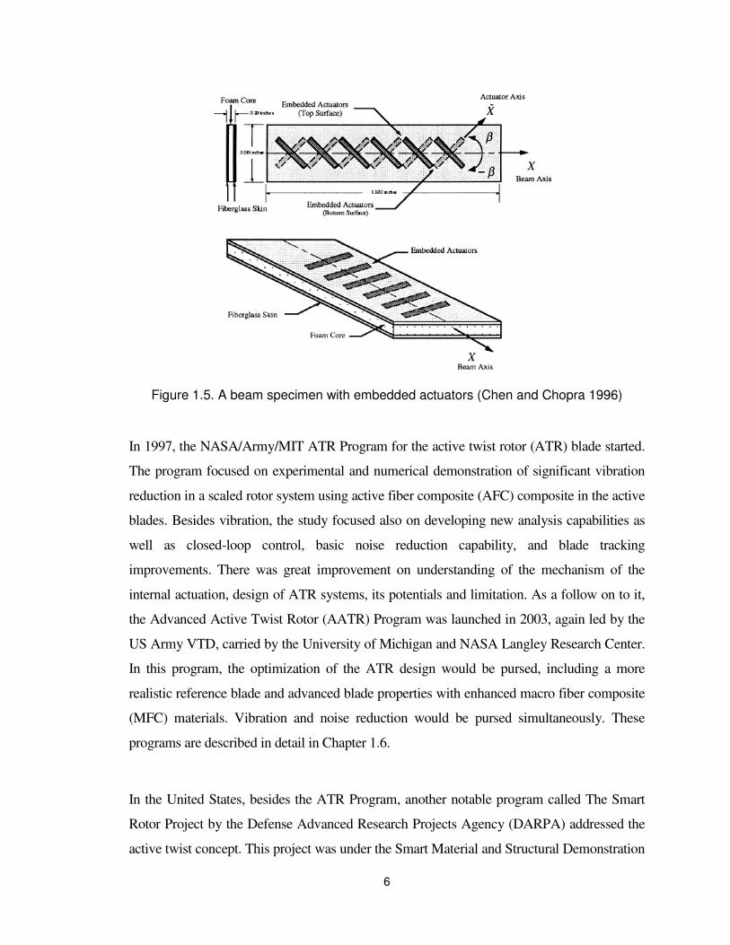
Figure 1.5. A beam specimen with embedded actuators (Chen and Chopra 1996) ................... 6

Figure 1.6. Single- or dual-ACF configuration used for vibration reduction (Friedmann 2004)

.................................................................................................................................................. 8

Figure 1.7. Sketch of Active Fiber Composite (Wickramasinghe and Hagood 2004) ............ 13

Figure 1.8. Fabrication of MFC Actuator (Wilkie et al. 2000) ................................................. 14

Figure 1.9. MFC Actuator (Wilkie et al. 2000) .......................................................................... 15

Figure 1.10. Aeroelastic Rotor Experimental System (ARES) testbed in Langley Transonic

Dynamics Tunnel (TDT) (Cesnik et al. 1999) .................................................................... 16

Figure 1.11. Final ATR-I prototype blade (Cesnik et al. 1999) ................................................ 17

Figure 1.12. The Langley Transonic Dynamics Tunnel ............................................................ 18

Figure 2.1. Illustration of active cross section showing ............................................................. 22

Figure 2.2. Flow chart of the design optimization framework .................................................. 23

Figure 2.3. Point mass with respect to the original and the output axes ................................... 28

Figure 2.4. Center of gravity with respect to the original and the output axes ......................... 29

Figure 3.1. (a) Planform and (b) cross section of the NASA/Army/MIT ATR-I blade .......... 33

Figure 3.2. Case A1 Optimization History ................................................................................. 38

viii

Figure 3.3. Case A2(a) optimization history for initial spar location at 0.2c............................ 43

Figure 3.4. Case A2(a) optimization history for initial spar location at 0.634c. ...................... 44

Figure 3.5. Case A2(b) optimization history for initial spar location at 0.2c. .......................... 46

Figure 3.6. Case A2(b) optimization history for initial spar location at 0.634c. ...................... 47

Figure 3.7. Case A3 optimization history ................................................................................... 49

Figure 3.8. Evolution of Case A3 (a) ply-thickness and (b) ply angles evolution ................... 50

Figure 3.9. Case A4 optimization history ................................................................................... 51

Figure 3.10. Army AH-64 Apache helicopter DoD photo by Petty Officer 3rd Class Shawn

Hussong, U.S. Navy. (Released) .......................................................................................... 55

Figure 3.11. ATR-A model blade planform (R = 60.48 inches. Not to scale.) ....................... 57

Figure 3.12. ATR-A Cross sectional view (VR18 with trailing edge tab) ............................... 57

Figure 3.13. Element overlapping close-up ................................................................................ 60

Figure 3.14. Discontinuity introduction at nose ......................................................................... 60

Figure 3.15. Trailing edge tab element modeling approach ...................................................... 61

Figure 3.16. Modified model for trailing edge tab ..................................................................... 61

Figure 3.17. MFC unit electrode layup ....................................................................................... 62

Figure 3.18. Inappropriate transition modeling .......................................................................... 62

Figure 3.19. Single ply model for electrode (pink) .................................................................... 62

Figure 3.20. Distorted quad element from mesh generator ....................................................... 63

Figure 3.21. Corrected quad element by PATRAN ................................................................... 64

Figure 3.22. Nose cross section mesh ......................................................................................... 65

Figure 3.23. Case T1(a) Optimization history ............................................................................ 70

Figure 3.24. Case T1(b) Optimization history ............................................................................ 72

Figure 3.25. Case T1(c) Optimization history ............................................................................ 74

Figure 3.26. Case T1(d) Optimization history ............................................................................ 76

Figure 3.27. Case T2(a) Optimization history ............................................................................ 78

Figure 3.28. Case T2(b) Optimization history ............................................................................ 80

Figure 3.29. Case T2(c) Optimization history ............................................................................ 82

Figure 3.30. Case T2(d) Optimization history ............................................................................ 84

ix

Figure 3.31. Case T1(b) Cross section layup .............................................................................. 86

Figure 3.32. Case T2(b) Cross section layup .............................................................................. 86

Figure 3.33 Span-wise optimization history – cross sectional design ...................................... 90

Figure 3.34. Span-wise Optimization history ............................................................................. 91

Figure 3.35. Torsional moment at 3P actuated, 45 phase angle ................................................ 94

Figure 3.36. Case Tu Optimization history ................................................................................. 97

Figure 3.37. Optimized Layup result for Case Tu ...................................................................... 98

Figure 3.38. Cross section sketch for layup with two ballast masses ..................................... 104

Figure 3.39 Schematic diagram of the ATR-I blade design (Shin 1999) ............................... 105

Figure 3.40. Position of ballast rods on leading edge of airfoil ............................................... 105

Figure 3.41. Possible geometry of ballast mass ........................................................................ 105

Figure 3.42. Case S1 Sectional distribution of strain due to unit torque (Γ12 per in-lbf) ....... 108




Figure 3.46. Active cross section for Case Tu2 showing layup definition ............................. 112

Figure 3.47. Detail of the cross section near the ballast mass location ................................... 112

Figure 3.48. Cross-Section of the root layup – Option 1 ......................................................... 115

Figure 3.49. Cross-Section sketch for the tip layup definition - Option 3 .............................. 116

Figure 3.50. Sectional distribution ............................................................................................ 118

Figure 3.51. Cross section sketch for layup definition (Section 0) ........................................ 119





Figure 3.56. Detailed of trailing edge tab ................................................................................. 122

Figure 3.57. Detailed view near the electrode (pink) ............................................................... 122

Figure 3.58. Nose zoom for proposed ply drop ........................................................................ 123

x

Figure 3.59. Modeling ply-drop on mesh-generator ................................................................ 123

Figure 3.60. Comparison of stiffness components ................................................................... 124

Figure 3.61. Comparison of mass components ........................................................................ 125

xi

LIST OF TABLES

Table 3.1. Material properties of the constituents in the ATR-I blades .................................... 34

Table 3.2. General target requirements for reference blade (considering heavy gas test

medium) ................................................................................................................................. 34

Table 3.3. Characteristics of the ATR-I blade ............................................................................ 35

Table 3.4. Constraints and bounds for Case A1 ......................................................................... 36

Table 3.5.Initial values of the design variables for Case A1 ..................................................... 37

Table 3.6. Reference and optimization results for Case A1 ...................................................... 39

Table 3.7. Constraints for cases with characteristics improved from the ATR-I baseline case

................................................................................................................................................ 40

Table 3.8. Initial design values of Case A2, A3 and A4 ............................................................ 41

Table 3.9 Optimized values for Case A2(a) ............................................................................... 42

Table 3.10. Optimized values for Case A2(b) for both initial conditions of spar location ...... 45

Table 3.11. Optimized results for Cases 2, 3 and 4 .................................................................... 52

Table 3.12. ATR-A blade target properties ................................................................................ 56

Table 3.13.Effects of unmodeled foam in the design of the active cross section ..................... 65

Table 3.14. Constraints used for the ATR-A optimization study .............................................. 67

Table 3.15. ATR-A optimization cases ....................................................................................... 68

Table 3.16. Case T1(a) Initial and optimized values .................................................................. 69

Table 3.17. Case T1(b) Initial and optimized values ................................................................. 71

Table 3.18. Case T1(c) Initial and optimized values .................................................................. 73

Table 3.19. Case T1(d) Initial and optimized values ................................................................. 75

Table 3.20. Case T2(a) Initial and optimized values .................................................................. 77

xii

Table 3.21. Case T2(b) Initial and optimized values ................................................................. 79

Table 3.22. Case T2(c) Initial and optimized values .................................................................. 81

Table 3.23. Case T2(d) Initial and optimized values ................................................................. 83

Table 3.24. ATR-A case study summary .................................................................................... 85

Table 3.25. Material Properties of the foam ............................................................................... 86

Table 3.26. Case T1(b) before and after the inclusion of foam ................................................. 87

Table 3.27. Case T2(b) before and after the inclusion of foam ................................................. 87

Table 3.28. Constraints and bounds for the span-wise optimization case ................................ 89

Table 3.29. Initial and optimized values for the span-wise optimization case ......................... 89

Table 3.30. Optimized length of the MFC for the different active sections ............................. 89

Table 3.31. Initial and optimized values of the span-wise optimization case .......................... 92

Table 3.32. Updated worst-case loading with optimized design ............................................... 95

Table 3.33.Constraints and bounds for Case Tu......................................................................... 96

Table 3.34. Case Tu Initial and optimized results ...................................................................... 98

Table 3.35. Mechanical properties of foam ................................................................................ 99

Table 3.36. Cases analyzed in foam study .................................................................................. 99

Table 3.37. Comparison with foam implementation for Case Tu1 ......................................... 100



Table 3.40. Comparison of with foam implementation cases ................................................. 103

Table 3.41. Case description ..................................................................................................... 106

Table 3.42. Common properties for sections 0, 1 & 2 ............................................................. 107

Table 3.43. Cross sectional properties (with foam) .................................................................. 107

Table 3.44. Strain values for worst case loads .......................................................................... 108

Table 3.45. Blade actuation properties ...................................................................................... 108

Table 3.46. Commercially available material properties provided by manufacturer ............. 110

Table 3.47. Baseline material properties ................................................................................... 111

Table 3.48. Active layer geometric information ...................................................................... 113

xiii

Table 3.49. Main blade cross sectional properties ................................................................... 113

Table 3.50. ATR-A blade root properties ................................................................................. 114

Table 3.51. Root cross sectional geometry and max strain component .................................. 115

Table 3.52. ATR-A Blade Tip Properties ................................................................................. 116

Table 3.53. Tip cross sectional geometry and maximum strain components ......................... 117

Table 3.54. Types of tungsten rods ........................................................................................... 118

Table 3.55. ATR-A blade properties ......................................................................................... 119

Table 3.56. ATR-A blade final design properties .................................................................... 126

xiv

LIST OF APPENDICES

Appendix 1. ATR optimization code structure ......................................................................... 133

Appendix 2. Maximum loads for ATR-I by CAMRAD II ..................................................... 134

Appendix 3. ATR-A blade lead-lag stiffness study ................................................................. 135

Appendix 4. Maximum loads for Case T1(b) by CAMRAD II .............................................. 136

Appendix 5. Refined ATR-A main blade mass stiffness and actuation matrices (SI unit) ... 138

Appendix 6. Refined ATR-A Root design mass and stiffness matrices (SI unit) .................. 139

Appendix 7. Refined ATR-A Tip layup mass and stiffness matrices (SI unit) ...................... 140

xv

ABSTRACT

This dissertation introduces the process of optimizing active twist rotor blades in the presence

of embedded anisotropic piezo-composite actuators. Optimum design of active twist blades

is a complex task, since it involves a rich design space with tightly coupled design variables.

The study presents the development of an optimization framework for active helicopter rotor

blade cross-sectional design. This optimization framework allows for exploring a rich and

highly nonlinear design space in order to optimize the active twist rotor blades. Different

analytical components are combined in the framework: cross-sectional analysis (UM/VABS),

an automated mesh generator, a beam solver (DYMORE), a three-dimensional local strain

recovery module, and a gradient based optimizer within MATLAB. Through the

mathematical optimization problem, the static twist actuation performance of a blade is

maximized while satisfying a series of blade constraints. These constraints are associated

with locations of the center of gravity and elastic axis, blade mass per unit span, fundamental

rotating blade frequencies, and the blade strength based on local three-dimensional strain

fields under worst loading conditions.

Through pre-processing, limitations of the proposed process have been studied. When

limitations were detected, resolution strategies were proposed. These include mesh

overlapping, element distortion, trailing edge tab modeling, electrode modeling and foam

implementation of the mesh generator, and the initial point sensibility of the current

optimization scheme.

xvi

Examples demonstrate the effectiveness of this process. Optimization studies were performed

on the NASA/Army/MIT ATR blade case. Even though that design was built and shown

significant impact in vibration reduction, the proposed optimization process showed that the

design could be improved significantly. The second example, based on a model scale of the

AH-64D Apache blade, emphasized the capability of this framework to explore the nonlinear

design space of complex planform. Especially for this case, detailed design is carried out to

make the actual blade manufacturable. The proposed optimization framework is shown to be

an effective tool to design high authority active twist blades to reduce vibration in future

helicopter rotor blades.

1

CHAPTER 1

INTRODUCTION

This chapter offers an introduction to the vibration reduction with actively controlled twist

blade, starting with some background and basic concepts for helicopter vibrations. Then the

related researches are reviewed; followed by a separate section about the active materials for

active twist blades and the Active Twist Rotor (ATR) blade program. Lastly, the scope and

the objectives of this dissertation are presented.

1.1 Background

Long before Leonardo Da Vinci drew the concept of a rotorcraft-like machine in 1483

(Figure 1.1), people had been fascinated by the idea of something flying in the manner of a

rotorcraft. The ancient Chinese had a hand-spun toy that rose upward when revolved rapidly

between hands (Figure 1.2).

Nowadays, the helicopter is used not only in the military but in various civilian fields such as

search-and-rescue from hard-to-reach areas, off-shore transportation, medical evacuation, etc.

However, it is not as widely used it should. There exist problems in rotorcraft that limit its

usage, one of the most important being fuselage vibration. Since each rotor blade is a slender,

flexible structure in a high unsteady flow, it undergoes elastic deformation and vibrate even

in normal operating conditions. This vibration can affect performance, reliability, noise,

fatigue on rotorcraft components and discomfort for passengers and, of course, increases

cost.

2

Figure 1.1. Da Vinci’s flying machine concept, manuscript B, folio 83 v., Courtesy of Bibliotheca Ambrosia

Figure 1.2. Chinese Bamboo Helicopters, circa 400 B.C. (Lemos 2007)

3

1.2 Helicopter vibration control

The primary source of many of the helicopter’s problems is the complex unsteady

aerodynamic environment which is generated near the rotor blades, mainly during forward

flight (Hooper 1984). The helicopter develops an instantaneous asymmetry of the

aerodynamic loads acting on the blades at different azimuth locations as it moves forward,

and such asymmetry becomes more and more adverse as the forward-flight speed increases.

Figure 1.3 shows a typical aerodynamic environment during forward flight. As a result of the

flight velocity that adds differently according to the azimuth angle to the blade rotating speed,

a high tip Mach number on the advancing side occurs, and blade stall affects the retreating

side. A reverse flow region is also generated, inboard on the retreating side. Aerodynamic

environment results in an instantaneous asymmetry of the aerodynamic loads acting among

the blades at different azimuthal locations. Due to this, a vibratory response happens on a

flexible blade structure, which makes the air loads more asymmetric, and this vibration

propagates to the fuselage through the hub.

Figure 1.3. Aerodynamic environment in forward flight (Wilkie 1997)

4

Vibration control has been studied from the very early years of helicopter development.

During the mid-1950s, development to reduce the vibration levels in the rotor led to designs

that included chord-wise and span-wise placement of concentrated masses, or tuning masses.

The traditional vibration reduction technique was a passive approach, with vibration isolators

and absorbers. Later, actively controlled vibration of helicopters emerged. This approach

reduces vibrations at their source in the main rotor before they propagate into the fuselage.

Higher Harmonic Control (HHC) is an active method implemented at the conventional

swashplate in the non-rotating reference frame. The unsteady aerodynamic loads on the

blades are redistributed by actively controlling the blade pitch angle at the root. Shaw et al.

tested the closed loop control with fixed gain controller, and it showed good performance up

to 25% of the desired service life for a full-scale production design (Shaw et al. 1989). An

alternative actively controlled vibration approach is the Individual Blade Control (IBC). In

this method, each blade is individually controlled in the rotating reference frame. This

approach is more general and may overcome the limitations found in HHC with the

conventional swashplate. The IBC concept has been implemented in such form as pitch

control actuation at the blade root.

Improved from the IBC concept, on-blade control methods emerged. The idea is still

controlling the blade individually but the control actuation occurs on each of the blades,

instead of the pitch-link at the root. The most popular concepts for that are the active

controlled flap (ACF) (Fulton and Ormiston 1998; Milgram and Chopra 1998; Friedmann et

al. 2001) and the active twist rotor blades (Rodgers and Hagood 1998; Cesnik et al. 1999),

both showing promising characteristics.

For conventional active control technology, the servo hydraulic actuator is commonly used.

Unfortunately, it is not suitable ideal for the on-blade control due to the following limitations:

multiple energy conversions, large number of parts, high vulnerability of the hydraulic pipe

network and the limited frequency bandwidth. Active materials are introduced to overcome

these limitations. The advantage of using active materials, particularly piezoelectric

5

materials, is a direct conversion from electrical to mechanical energy with high-frequency

response. Electric energy is easier to transmit, and electric lines are much less vulnerable to

damage than hydraulic pipes. Though piezo-electric active materials have large force and

energy capabilities, induced strain actuators have a relatively small stroke where the

displacement amplification mechanism is needed.

1.3 On-blade actuation concepts

The development of active twist rotor blades incorporating piezo-ceramic materials in order

to enable an individual twist deformation of the rotor blades started in the early 1990s. The

first attempt at designing active twist blades was presented by Barrett in his master thesis

(Barrett 1990) using directionally placed piezo-electric crystals (Figure 1.4). Chen and

Chopra updated this idea to introduce strain directly by embedding thin monolithic

piezoelectric actuators under the fiber-glass skin of the blade as in Figure 1.5. They suggested

to apply the strain at a 45° angle with respect to the blade axis for maximum actuation (Chen

and Chopra 1996).

Figure 1.4. Arrangement of Directionally Attached Piezo-electic (DAP) actuator element on the blade prior to fiberglass application (Barrett 1990)

6

Figure 1.5. A beam specimen with embedded actuators (Chen and Chopra 1996)

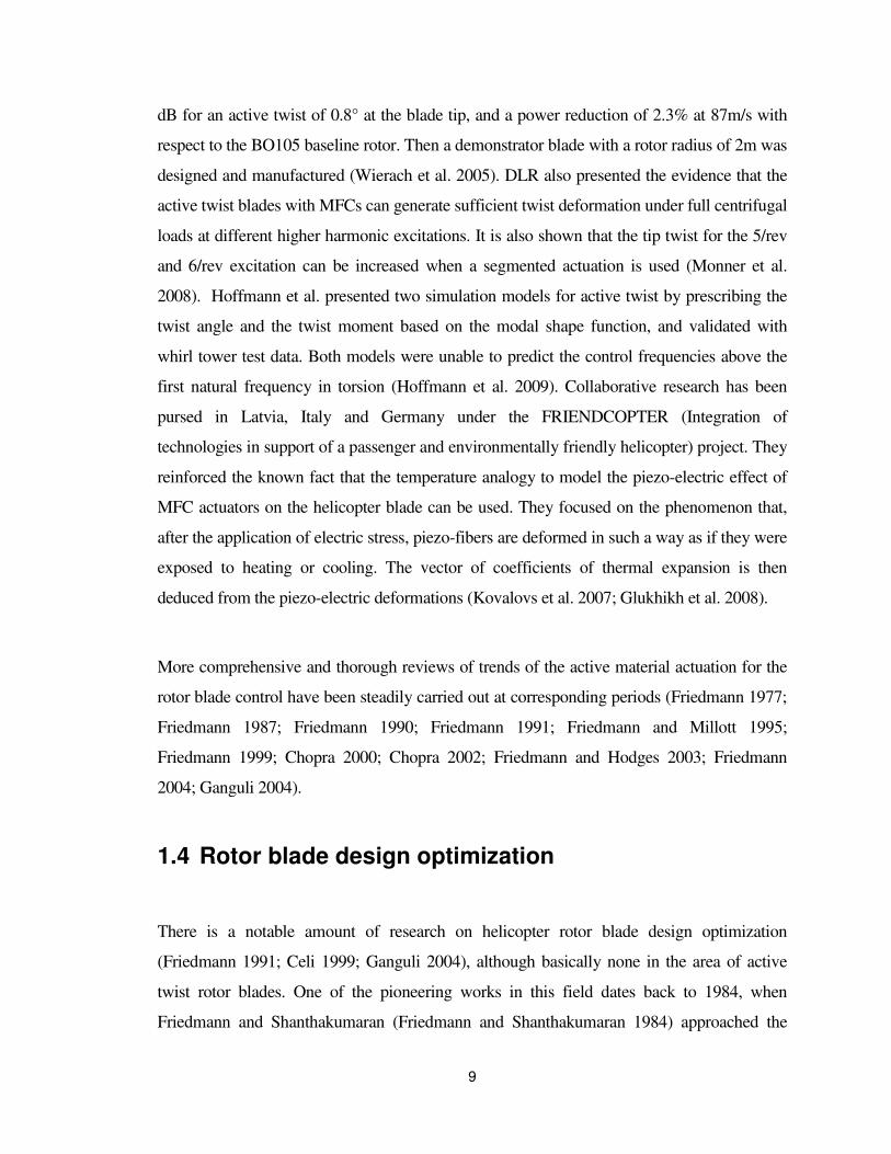
In 1997, the NASA/Army/MIT ATR Program for the active twist rotor (ATR) blade started.

The program focused on experimental and numerical demonstration of significant vibration

reduction in a scaled rotor system using active fiber composite (AFC) composite in the active

blades. Besides vibration, the study focused also on developing new analysis capabilities as

well as closed-loop control, basic noise reduction capability, and blade tracking

improvements. There was great improvement on understanding of the mechanism of the

internal actuation, design of ATR systems, its potentials and limitation. As a follow on to it,

the Advanced Active Twist Rotor (AATR) Program was launched in 2003, again led by the

US Army VTD, carried by the University of Michigan and NASA Langley Research Center.

In this program, the optimization of the ATR design would be pursed, including a more

realistic reference blade and advanced blade properties with enhanced macro fiber composite

(MFC) materials. Vibration and noise reduction would be pursed simultaneously. These

programs are described in detail in Chapter 1.6.

In the United States, besides the ATR Program, another notable program called The Smart

Rotor Project by the Defense Advanced Research Projects Agency (DARPA) addressed the

active twist concept. This project was under the Smart Material and Structural Demonstration

7

Program (Sanders 2004), the second phase of the DARPA program which initiated in 1993

after DARPA realized the importance and impact of smart material technology in aerospace

systems. The Boeing/MIT team introduced two concepts. One was the concept to use the

trailing edge flap to induce the blade twist, and the other was to use embedded piezoelectric

composite to twist the blade directly. They implemented these concepts on 1/6th Mach scale

model of CH47D Chinook blade (Rodgers 1999; Prechtl 2000).

Other research groups are doing different research related to the active blade control. The

Pennsylvania State University team suggested that the induced shear piezoelectric tube

actuator, which is the torsional PZT actuator for ATR blades, to be used to twist the blades

(Centolanza 2002). Prahlad and Chopra developed the methodology to model and explore the

torsional actuator with shape memory alloy (SMA) actuators (Prahlad and Chopra 2007).

One of the most extensively explored approaches in this research area is the actively

controlled flap (ACF). Friedmann and Millott demonstrated the potential of AFC for

vibration reduction in helicopters in forward flight (Millott and Friedmann. 1994; Friedmann

and Millott 1995). The ACF implements small partial-span trailing-edge flap either in the

single flap or dual-flap configuration, as shown in Figure 1.6. Fulton and Ormiston presented

the experimental results on the practical implementation of the ACF and its application to

fundamental vibration reduction in the open-loop mode, on a two-bladed rotor. These results

enabled to compare the simulation to the obtained experimental data (Fulton and Ormiston

1998). Through the papers about practical implantation of AFC, important problem has been

noticed that the maximum flap deflections can reach 15 deg, which is larger than angles that

can be achieved with active or smart materials-based actuation. In addition, practically the

flap authority will have to be limited to 3–4 deg to avoid interfering with the handling

qualities of the helicopter. Cribbs and Friedmann proposed new control method with limited

flap deflections, 4 deg. This method showed that a hub vibration reduced as similar to the

ones without limiting the flap deflections (Cribbs and Friedmann 2001). Additional studies

on the single and dual ACF systems have been conducted. As expected, the dual-flap

configuration showed better effectiveness in alleviating the vibration than the single-flap

configuration (Depailler and Friedmann 2002). Milgram and Chopra performed the

8

parametric studies on vibration reduction using actively controlled flaps and showed that the

flap system significantly reduced the fixed system 4/rev hub loads (Milgram and Chopra

1998).

Figure 1.6. Single- or dual-ACF configuration used for vibration reduction (Friedmann 2004)

Meanwhile, from 1994 to 2001, the Japanese government agencies conducted experiments

on the active flap using an electromagnetic actuator. The Japan Aerospace Exploration

Agency (JAXA) has presented the effectiveness of the active flap control on BVI (Blade

Vortex Interaction) noise reduction (Aoyama et al. 2006). They presented the evidence that

the active flap control is as effective as IBC with a small control area, which is only 4.5% of

IBC.

In Europe, DLR (German Aerospace Center) and ONERA (French National Aerospace

Research Center) have also been jointly pursuing a similar project (Philippe 2003). They

investigated the active flaps and active twist rotors and presented the potentials of each.

Brockmann and Lammering in Germany developed a three-dimensional beam finite element

for further investigation with anisotropic actuation in the rotating beam (Brockmann and

Lammering 2006). DLR developed a detailed structural model on the basis of the BO105

model rotor blade, to predict the performance with respect to rotor-dynamics, stability,

aerodynamics and acoustics. These rotor dynamic simulations showed a noise reduction of 3

9

dB for an active twist of 0.8° at the blade tip, and a power reduction of 2.3% at 87m/s with

respect to the BO105 baseline rotor. Then a demonstrator blade with a rotor radius of 2m was

designed and manufactured (Wierach et al. 2005). DLR also presented the evidence that the

active twist blades with MFCs can generate sufficient twist deformation under full centrifugal

loads at different higher harmonic excitations. It is also shown that the tip twist for the 5/rev

and 6/rev excitation can be increased when a segmented actuation is used (Monner et al.

2008). Hoffmann et al. presented two simulation models for active twist by prescribing the

twist angle and the twist moment based on the modal shape function, and validated with

whirl tower test data. Both models were unable to predict the control frequencies above the

first natural frequency in torsion (Hoffmann et al. 2009). Collaborative research has been

pursed in Latvia, Italy and Germany under the FRIENDCOPTER (Integration of

technologies in support of a passenger and environmentally friendly helicopter) project. They

reinforced the known fact that the temperature analogy to model the piezo-electric effect of

MFC actuators on the helicopter blade can be used. They focused on the phenomenon that,

after the application of electric stress, piezo-fibers are deformed in such a way as if they were

exposed to heating or cooling. The vector of coefficients of thermal expansion is then

deduced from the piezo-electric deformations (Kovalovs et al. 2007; Glukhikh et al. 2008).

More comprehensive and thorough reviews of trends of the active material actuation for the

rotor blade control have been steadily carried out at corresponding periods (Friedmann 1977;

Friedmann 1987; Friedmann 1990; Friedmann 1991; Friedmann and Millott 1995;

Friedmann 1999; Chopra 2000; Chopra 2002; Friedmann and Hodges 2003; Friedmann

2004; Ganguli 2004).

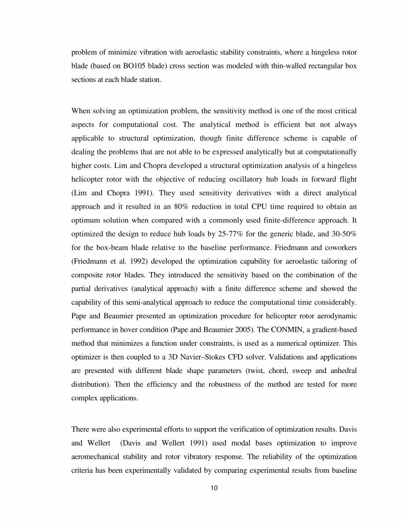
1.4 Rotor blade design optimization

There is a notable amount of research on helicopter rotor blade design optimization

(Friedmann 1991; Celi 1999; Ganguli 2004), although basically none in the area of active

twist rotor blades. One of the pioneering works in this field dates back to 1984, when

Friedmann and Shanthakumaran (Friedmann and Shanthakumaran 1984) approached the

10

problem of minimize vibration with aeroelastic stability constraints, where a hingeless rotor

blade (based on BO105 blade) cross section was modeled with thin-walled rectangular box

sections at each blade station.

When solving an optimization problem, the sensitivity method is one of the most critical

aspects for computational cost. The analytical method is efficient but not always

applicable to structural optimization, though finite difference scheme is capable of

dealing the problems that are not able to be expressed analytically but at computationally

higher costs. Lim and Chopra developed a structural optimization analysis of a hingeless

helicopter rotor with the objective of reducing oscillatory hub loads in forward flight

(Lim and Chopra 1991). They used sensitivity derivatives with a direct analytical

approach and it resulted in an 80% reduction in total CPU time required to obtain an

optimum solution when compared with a commonly used finite-difference approach. It

optimized the design to reduce hub loads by 25-77% for the generic blade, and 30-50%

for the box-beam blade relative to the baseline performance. Friedmann and coworkers

(Friedmann et al. 1992) developed the optimization capability for aeroelastic tailoring of

composite rotor blades. They introduced the sensitivity based on the combination of the

partial derivatives (analytical approach) with a finite difference scheme and showed the

capability of this semi-analytical approach to reduce the computational time considerably.

Pape and Beaumier presented an optimization procedure for helicopter rotor aerodynamic

performance in hover condition (Pape and Beaumier 2005). The CONMIN, a gradient-based

method that minimizes a function under constraints, is used as a numerical optimizer. This

optimizer is then coupled to a 3D Navier–Stokes CFD solver. Validations and applications

are presented with different blade shape parameters (twist, chord, sweep and anhedral

distribution). Then the efficiency and the robustness of the method are tested for more

complex applications.

There were also experimental efforts to support the verification of optimization results. Davis

and Wellert (Davis and Wellert 1991) used modal bases optimization to improve

aeromechanical stability and rotor vibratory response. The reliability of the optimization

criteria has been experimentally validated by comparing experimental results from baseline

11

and optimized rotors. Young and Tarzanin (Young and Tarzanin 1993) performed a Mach-

scaled wind tunnel test to validate a four-bladed low vibration rotor design for two different

rotors as above - One for the reference rotor, similar to a scaled Model 360 and for the low

vibration rotor designed by analytical optimization procedure. The test showed the 4/rev

vertical hub load and moments reduction for the optimized low vibration rotor.The research

extended its footage to the optimization on the active blade design. Viswamurthy and

Ganguli studied the effect of the multiple active trailing edge flaps for vibration reduction in a

helicopter rotor using an optimization approach (Viswamurthy and Ganguli 2004). When

only the vibration reduction is considered, the gradient-based optimization example showed

that four active trailing edge flaps at the blade tip with at higher harmonic actuations reduced

the vibration about 72% in forward flight. By the tradeoff studies between vibration reduction

and control deflections for one, two and four active trailing edge flaps, using four trailing

edge flaps at the blade tip (outer 20%) was optimal for reducing vibration with low control

angle deflections which requires low power. More recently, Glaz et al. (Glaz et al. 2006)

showed the effectiveness of surrogate modeling of helicopter vibrations, and the use of the

surrogates for optimization of helicopter vibration. Glaz then extended that study to what he

calls a “passive/active approach” (Glaz 2008). He demonstrated that the efficient global

optimization algorithm showed better performance than the conventional surrogate based

optimization techniques for vibration reduction at low speed forward flight. Then Actively

Controlled Flap was introduced to further reduce vibration and noise, and enhance

performance. This active/passive design showed 68 – 91 % reductions in vibration and a 2.3 -

2.7 dB decrease in the maximum noise level. In Europe, DLR proposed a new concept for

individual blade control: the Active Trailing Edge (ATE) which has a similar effect as in

trailing edge flaps (Grohmann et al. 2008). Detailed aero-servo-elastic optimization and

sensitivity studies have been presented. The aero-servo-elastic optimization of the ATE

actuator is based on an evolutionary algorithm. It has been demonstrated that the thickness of

piezo-ceramic layers is a key parameter for optimization. They showed similar performance

for reduction of vibration as did the previously developed trailing edge servo flap.

1.5 Active materials for active twist rotor blades

The active materials, that are also commonly called smart materials, have one or more

12

properties that change by a controllable external input, such as stress, temperature, pH

(acidity), electric or magnetic fields, and moisture. There are a number of types of active

materials, some of which are already commonly used. Shape memory alloy might be the

most popular one whose deformation is induced and recovered through temperature changes.

Electrorheological (ER) and magnetorheological (MR) materials are fluids, which can

experience a dramatic change in their viscosity when in the presence of an electric or

magnetic field, respectively. Piezo-electric materials produce a voltage when mechanical

stress is applied and vice versa. Since it changes a structural property (stress) by a relatively

easily controllable input (electric field), it is a very strong candidate for structural control

application. There are basically two types of piezoelectric materials. One is piezo-ceramic

(PZT) and the other is piezo-film (PVDF). They are already widely used in practice. For

example, inside a microphone, a piezo-film translates the variation of air pressure from sound

to electrical signals. PVDF is commonly used as a sensor. It cannot produce significant force

but is flexible enough to be placed on curved surfaces. On the other hand, PZT is used as an

actuator due to its relatively high strength. In short, PZT has strength without flexibility and

PVDF has flexibility without strength.

The active twist rotor blade actuator requires certain characteristics. First, it needs to be

flexible enough to be incorporated into the curved shape of the blade. It is also expected to

have enough structural integrity to withstand the pressure applied during blade fabrication

and the external loads during blade operation. It must have high strain-inducing capabilities

in an appropriately applied electric field and anisotropy of the actuation is required so that

tailoring in the blade design may be possible. Thus, it can be said that, in an active twist rotor

blade, the materials need to be strong like piezoelectric ceramics but also flexible like the

film.

To solve this conflict, the active fiber composite (AFC) was developed (Bent et al. 1995).

AFC is a conformable anisotropic actuator, which can be integrated into a passive structure.

The AFC actuator is made with the inter-digitated electrode poling and piezoelectric fibers

embedded in an epoxy matrix. Figure 1.7 shows the lay-out of the AFC actuator. This

approach produces a high performance piezoelectric actuator laminate with both strength and

13

flexibility. Basic material characterization and the concept of an integral twist-actuated rotor

blade was investigated during the DARPA/Boeing/MIT integral actuated blade program

(Bent and Hagood 1997).

Figure 1.7. Sketch of Active Fiber Composite (Wickramasinghe and Hagood 2004)

More recently, the macro fiber composite (MFC) has been developed at NASA Langley

based on the same idea as the AFC, using the piezoelectric fibers under inter-digitated

electrodes. It is composed of a rectangular cross-section, with unidirectional piezo-ceramic

fibers that are embedded into a thermosetting polymer matrix and sandwiched between

Kapton sheets layered with copper inter-digitated electrodes. The fiber sheets are formed

from monolithic piezo-ceramic wafers and conventional computer controlled wafer-dicing

methods. The fabrication process is shown in Figure 1.8. They suggested adapting to

accommodate any piezo-ceramic material, dielectric film, electrode geometry, or matrix

adhesive, depending on the intended application, since the manufacturing process was

uniform and repeatable. Total cost for the baseline MFC device has proven to be as low as

approximately $120 (2000 US dollars) apiece at a “laboratory scale” (Wilkie et al. 2000), and

due to the ease of automation of manufacturing process, it can be reduced further by mass

production. Tests were performed to present the evidence of the capability and endurance of

the MFC. It produced large directional in-plane strains; around 2000µε under a 4000V peak-

14

to-peak applied voltage and endured up to 90 million electrical cycles without any reductions

in free-strain performance. Figure 1.9 shows a MFC actuator manufactured at NASA

Langley (Wilkie et al. 2000). In short, while the piezo-ceramic fibers in AFC are extruded,

the piezoelectric fibers in MFC are manufactured from dicing low-cost monolithic piezo-

ceramic wafers. Thus, it retains beneficial features of the AFC with a lower fabrication cost.

This actuator was tested for its characteristics (Williams et al. 2004; Williams et al. 2006) and

it has been considered for use in many aerospace applications.

a) 3.375 x 2.25 x 0.007 inch piezoceramic

wafer on polymer film

b) Computer-controlled dicing saw used for

cutting wafers.

c) Piezo-ceramic wafer and polymer film frame positioning for cutting.

d) Sheet of piezo-ceramic fibers, after

cropping from excess polymer film

Figure 1.8. Fabrication of MFC Actuator (Wilkie et al. 2000)

15

Figure 1.9. MFC Actuator (Wilkie et al. 2000)

1.6 Active twist rotor (ATR) project

In order to reduce high vibration levels, integral twist actuation of the rotor blades has been

proposed, which would have several potential benefits over other methodologies. As having

the blade using this design maintains a smooth and continuous surface along the blade, so

ATR blades do not interfere with aerodynamics as much as other methods. By controlling the

twist of each rotor blade individually, local changes to the vibratory loads are induced. This

results in a reduction of the vibrations transmitted to the fuselage through the rotor hub. With

the development of the AFC, the NASA/Army/MIT active twist rotor program was launched

in 1997 (Cesnik et al. 1999). In the ATR program, analysis and design methodologies were

developed for active blades with embedded piezo-composite actuators (Cesnik and Shin

2001).

An ATR prototype blade was designed and fabricated for bench/hover testing (Cesnik et al.

1999; Shin and Cesnik 1999; Wilkie et al. 1999; Cesnik et al. 2001). The test-bed for the

ATR blade is shown in Figure 1.10, and the final blade is presented in Figure 1.11. Following

these studies, a set of active blades was manufactured and wind tunnel tested in forward

flight (Wilbur et al. 2002). The open-loop (Wilbur et al. 2001; Wilbur et al. 2001) and

closed-loop controls (Bernhard and Wong 2003; Shin et al. 2005) in the forward flight test

showed significant authority and was successfully tested in Langley’s Transonic Dynamics

16

Tunnel (Cesnik et al. 1999). The blade design was explored with several design variables

based on an existing passive blade. Design variables such as the number of active layers,

length of the active region in the chord-wise direction, and the location of the active layers

that are inserted in the cross section, were varied. The other blade design parameters were

kept in an appropriate range to maintain characteristics similar to the baseline blade. The

design that showed the largest static twist actuation was selected for the final design.

Different studies also showed numerical and experimental evidence that varying the

distribution of passive and active materials in the cross section can improve the blade twist

actuation authority (Cesnik and Shin 2001; Cesnik et al. 2003). The basic acoustic feature of

ATR on noise reduction also was studied (Booth and Wilbur 2004). Shin continued his work

on ATR blades (Shin and Cesnik 2007; Shin et al. 2007; Shin et al. 2008).

Figure 1.10. Aeroelastic Rotor Experimental System (ARES) testbed in Langley Transonic Dynamics Tunnel (TDT) (Cesnik et al. 1999)

17

Figure 1.11. Final ATR-I prototype blade (Cesnik et al. 1999)

Encouraged by the results of this first phase, a new phase for the active twist rotor, the

Advanced Active Twist Rotor (AATR), was launched with the introduction of MFC in 2003.

As mentioned earlier, MFC is similar to AFC with the advantage in manufacturing and

corresponding costs. The objective of the original ATR program was to prove the feasibility

of an active-twist concept. It used a basic model (a rectangular blade planform with a NACA

0012 airfoil) for which several studies existed. The ATR performance was studied with

carefully chosen design variables. In spite of remarkable results, the manual iterative design

was not only time consuming but also was unable to guarantee the optimum result. It relied

on the designer’s understanding and experience of the existing blades. However, due to the

complexity of the ATR blade, its performance did not follow conventional expectations, as

shown by Cesnik and Shin (Cesnik and Shin 2001).

18

Figure 1.12. The Langley Transonic Dynamics Tunnel

The goal of the AATR design is to exploit current trends in blade design, such as advanced

blade tip geometry and high performance airfoils, as well as an optimized structural design,

in order to increase active-twist blade response while improving the passive (unactuated)

performance of the rotor (Cesnik et al. 2004; Cesnik et al. 2005). Recently, a parametric

study for an Advanced ATR was conducted by the U.S. Army Vehicle Technology

Directorate at NASA Langley Research Center (Sekula 2005). They performed an analytical

study to determine the impact of blade structural properties on active-twist performance. The

chosen parameters were blade torsional, flap-wise, and lag-wise stiffness; section mass;

torsional inertia; center of gravity; and elastic axis location. The effect of those parameters

on rotor power requirements, blade loads, and vibratory hub loads were studied.

1.7 Objectives and orgarnization of this dissertation

As one can see from the discussions presented above, the process to optimize active twist

blades is very complex. It adds to the already rich design space of traditional (passive)

helicopter blades with tightly coupled design variables and constraints. It seems natural to

invoke the principles of mathematical optimization to enable a reliable way to explore the

design space. This dissertation has the objective to develop an optimization design

framework for active twist helicopter blades with anisotropic piezo-composite materials (e.g.,

19

AFC and/or MFC) embedded in the composite construction for twist actuation. This

framework needs to incorporate appropriate analyses tools into an effective optimizer while

ensuring the required data flow among those tools. This is also to be done in a way to achieve

low computational expense and stable optimization process. Finally, this dissertation will

explore different ATR designs and their dependency on design parameters/variables to better

understand the drivers for high-authority active twist blades. This is done through the

numerical exploration of the large and complex design space which can take one much

further than the manual iterative design approach followed up to now.

This dissertation is structured so that Chapter II introduces the new framework to optimize

the design of active twist rotor blades with embedded active actuators. The mathematical

statement of the optimization problem is presented and the descriptions for each component

of the framework followed in detail. Chapter III presents numerical studies using the

proposed optimization approach on active twist blades. The first part of that chapter

demonstrates the capabilities of this optimization framework with the NASA/Army/MIT

ATR blade. The optimization cases based on this blade are performed with different sets of

design variables and constraints. Then a more realistic problem based on a model-scale blade

of the AH-64D Apache helicopter is used to show further capabilities of the proposed

optimization framework. Prior to perform the optimization, further capabilities and

limitations of the code are studied and addressed. Then the optimization cases with different

constraints and different set of design variables are performed and the results are studied in

detail. One of the designs is selected and refined for later manufacturing. In Chapter IV, the

main contributions of this thesis are summarized and future possible directions of research

are suggested.

20

CHAPTER 2

FRAMEWORK AND METHODOLOGY OF ATR

OPTIMIZATION

This chapter introduces the proposed framework to optimize the design of an active twist

rotor blade with embedded piezo-composite actuators. The chapter begins with the

mathematical statement of the optimization problem. Then the proposed framework for ATR

optimization is shown with a flowchart. The descriptions for each component of the

framework follow.

2.1 Optimization problem setup

The optimum blade design can be obtained by adjusting the design variables within the

physical or design required constraints. These variables and constraints are discussed in detail

below.

Mathematically, an optimization problem generally is stated as follows: Extremize the

desirable objective function f, according to the set of design variables x within certain limits,

while satisfying nonlinear constraints g. That is,

max f ( x )

(2.1)

subject to:

≤ 0g( x ) (2.2)

≤ ≤l u

x x x . (2.3)

where xl is the lower limit and xu the upper limit of the set x. For the ATR blade

optimization, the objective function f is the active twist induced by the embedded actuators.

Even though the vibration reduction is not directly connected or linearly dependent to the

21

twist actuation authority, it is known that vibration level reduces in proportion to the increase

of the twist actuation authority in the reasonable range.

The main design variables introduced in this optimization problem are:

• The thickness and lamination angle of each ply in the cross-section layup. The

material properties used in each ply, however, must be chosen in advance;

• The starting and ending locations of the active region along the cross-section;

• The chord-wise location of the spar (web) wall;

• The length of the spar web extensions;

• Two discrete ballast weights with their masses and chord-wise locations;

These variables may be introduced at different blade radii, and they may be linked within a

given span-wise region or among different regions of the blade. In setting up this problem,

the blade planform is subdivided into four regions of predetermined length. Each region may

have a different airfoil. The most outboard region represents the blade tip, and its cross-

sectional layup may be linked with the one from the neighboring inboard region. The blade

planform includes pre-twist and tip droop/sweep, in order to model modern helicopter blade

configurations. Figure 2.1 shows an illustration of active cross section showing (a) initial

layup configuration and (b) some of the design variables.

Due to manufacturing constraints, the chord-wise location of the spar web should be

considered a single design variable along the blade radius. If more parameters needed to be

linked because of practical manufacturing considerations, they could have been

accommodated as well. Finally, the permissible range of each design variable type is also

imposed based on practical considerations.

The following set of constraints (g(x)) is implemented in the proposed framework:

• Chord-wise location of the cross-sectional center of gravity;

• Chord-wise location of the cross-sectional elastic axis;

22

• Blade mass per unit span (for correct Lock number);

• Blade fundamental rotating frequencies (for desirable blade dynamics);

• Maximum allowable blade local strain under the worst-case loading condition

(associated with the ultimate strength of the constituent materials).

Besides these, additional constraints may be added to better pose the problem and make it

more realistic (see Chapter 3.1 ). Also, fatigue life is only considered indirectly by keeping

the dynamic strain levels below a practical threshold.

E-Glass 0°/90°S-Glass 0°/90°E-Glass 0°/90°E-Glass 0°/90°

E-Glass 0°/90°MFC +45°E-Glass +45°/-45°MFC -45°E-Glass 0°/90°

E-Glass 0°/90°E-Glass 0°/90°

E-Glass 0°/90°

E-Glass 0°/90°S-Glass 0°/90°E-Glass 0°/90°E-Glass 0°/90°

E-Glass 0°/90°MFC +45°E-Glass +45°/-45°MFC -45°E-Glass 0°/90°

E-Glass 0°/90°E-Glass 0°/90°

E-Glass 0°/90°

(a)

Ballast weight location

Start/end location of active plies

Spar location


Start/end location of active plies

Spar location

(b)

Figure 2.1. Illustration of active cross section showing

(a) initial layup configuration, and (b) some of its design variables

23

2.2 Optimization framework

Figure 2.2. Flow chart of the design optimization framework

(light grey area indicates inner loop while deeper shaded area is outer loop)

The proposed optimization framework is schematically described in Figure 2.2. Note that the

framework is composed of a two-level nested loop. The aeroelastic analysis is usually

computationally expensive and this is a very important factor in numerical optimization. So

for the inner loop, the maximum loads (two bending moments, torsion moment, two shear

forces, and axial force) for different flight conditions for pre-determined points along the

blade radius and azimuthal stations are kept constant. This is based on the assumption that the

structural design changes along the optimization process would not have much effect on the

worst loads on the blade. The inner loop undergoes several optimization cycles before the

design comes to the upper loop. Loads are recalculated and the process resumes until the

worst loads converge. Besides the two-nested optimization loops, pre-processing of the

model in preparation for the optimization and post-processing/analysis of the optimized

design at the very end are also part of the overall design process.

24

2.2.1 Pre-processing

To insure a smooth start for the optimization process, a reasonable baseline design is

expected. This is especially important for the optimization scheme that is adopted in this

framework. The baseline does not need to be feasible, but the constraints should not be

strongly violated. This can be achieved by using an initial design based on an existing blade

or previous designer’s experience. Also, the optimization framework can be used to guide the

design through few multidisciplinary analysis cycles and provide valuable information to the

designer to adjust the blade parameter before it goes to the next phase of the process.

The initial set of constraints must be chosen from the available set (see Section 2.1). Some of

the design parameters are fixed, including the length of the blade and airfoil type along the

blade. Others need to be initialized (e.g., layup stacking sequences along the blades, set of

materials) and may be varied during the optimization (e.g., ply angles, ply thicknesses, spar

web location, etc.).

Before the optimization process actually starts, potential problems are addressed in this phase

of the framework so to increase the likelihood of a smooth optimization run. The limitation

and the sensitivity of the solution are explored including, but not limited to, the quality of the

mesh used for every cross section sampled along the blade radius (particularly due to mesh

robustness when ply thickness becomes too small), the range of ply angles and materials used

as part of the seed laminate, sensitivity and robustness of the optimization scheme on initial

condition, etc.

2.2.2 Outer loop

As mentioned above, the aeroelastic load analysis is being brought out from the detail

laminate optimization (inner loop) cycle. Based on the initial (baseline) design, sets of loads

are calculated associated with different flight conditions (advance ratio, altitude, maneuvers).

These loads are represented in the form of rotating blade loads: two bending moments,

25

torsional moment, two shear forces, and the axial force, and they are typically given at

several blade radial stations and azimuthal positions. From all these load cases, for a given

blade station a critical load component is identified by scanning all azimuthal angles. At that

point, along with the critical load component, all the remaining components of the load case

are kept to form an entry on the critical loading set. This is done for all six load components

at a given radial station and then repeated for all radial positions along the blade and for all

flight conditions being considered. The critical loading set is then passed to the inner loop for

structural sizing. Once the inner loop optimization cycle is completed, a new set of blade

parameters are received by the outer loop from which new aeroelastic load analyses are

performed. This process continues until the blade design and critical load set converge, at

which point the design is considered ready for the post-processing phase. This separation of

the aeroelastic analysis from the structural optimization process (inner loop), reduces the

computational cost remarkably without affecting the structural design significantly. In this

dissertation, the aeroelastic load analysis was performed using CAMRAD II by NASA

Langley.

2.2.3 Inner loop

(1) Optimization scheme

The inner loop optimization code is developed on the MATLAB planform, due to its

capability of adopting/combining other codes and easy of use. Moreover, MATLAB provides

optimization solutions in its framework. and “fmincon” was chosen from its optimization

toolbox. The “fmincon” function minimizes a constrained nonlinear multivariable problem.

A gradient-based constrained optimization scheme is desirable due to its flexibility to deal

with large, nonlinear problems. The “medium scale” option is used, which is associated with

a sequential quadratic programming method. For each iteration, the function solves a

quadratic programming sub-problem, which improves convergence (Hafka and Gurdal

1992). The gradients of the objective function and the constraints are provided from finite

differentiation (implemented in the framework). The BFGS (Broyden-Fletcher-Goldfarb-

Shanno) method (Fletcher and Powell 1963), a well-known quasi-Newtonian algorithm for

unconstrained optimization, is applied to this method. Three kinds of termination criteria

26

have been used: maximum number of iterations, tolerance on the design variables, and

tolerance on the objective function value. When one of these termination criteria is satisfied,

the optimization loop will end. In case the result indicates that the solution still needs further

iterations, with different constraints, the optimization can be restarted from the point where it

stopped previously. This restart feature enables using the history of prior optimization and

reduces the computational cost.

Since the objective function of this problem is highly nonlinear, and since the design

hyperspace is very complex, it is possible for “fmincon” to fall into a local extremum, leading

to a sub-optimal solution. Therefore, it is necessary to run the optimization to completion,

starting from different initial points. Furthermore, when the problem is infeasible, “fmincon”

attempts to reduce the distance to the most violated constraint boundary. To simplify this step

and add robustness to the procedure, it is recommended to start with a feasible initial point if

possible.

(2) 2-D Cross sectional analysis

UM/VABS (Cesnik and Palacios 2003) is a finite-element based analysis of active cross

sections with arbitrary geometry and material distributions. UM/VABS (University of

Michigan–Variational-Asymptotic Beam Section analysis) can compute the cross-sectional

elastic, inertial, thermal, and electric characteristics of active anisotropic beams of arbitrary

cross-sectional shape, including the effects of initial twist and curvature. In this optimization

process, UM/VABS provides cross-sectional stiffness, inertia and actuation forces/moments

values to be used in the one-dimensional (beam) modeling of the blade. It also calculates the

locations of the center of gravity and elastic axis, the blade mass per unit span, and the static

active twist rate (in a given cross section). UM/VABS input has a NASTRAN-based format.

It also has a Timoshenko-like beam option and this gives the 6×6 stiffness matrix as output

based on extension, transverse shear in two directions, twist, and bending curvature in two

directions, accordingly. The 6×6 inertia matrix is based on 3 displacements and 3 rotations.

Further explanation and mathematical background can be found in (Palacios Nieto 2005).

Since UM/VABS would be included in the optimization process, it is crucial to have an

27

automated mesh generator that can take a few parametric inputs and generate the needed

mesh. This is accomplished with a MATLAB-based mesh generator specially developed for

UM/VABS. To create a general airfoil wetted surface, pairs of coordinate points defining the

contour of the airfoil must be supplied. Contour equations have been implemented for the

NACA four- and five-digit series airfoils. Otherwise, the contour can be supplied from a

lookup table. From the wetted surface, layers of given (composite) material are defined in

order to create the stacking sequence needed for the internal structural configuration.

Materials are defined for every passive and active layer. Using a look-up table, their

properties are loaded for each layer. Although UM/VABS can deal with any type of internal

cross-sectional geometry, the mesh generator is limited to modeling walls and webs only (no

foam or honeycomb filling, for example). The inertial effects associated with the ballast

masses are added directly to the inertia matrix generated in UM/VABS:

Mass moment of inertia matrix is defined as follows.

−im

mm

ξξ

~

~= M

(2.4)

When implement the effect of the ballast weight Mp to the mass matrix, it should be

considered that the output reference axes is parallel to the principal area axes in the

UM/VABS setup for the Timoshenko-like model where the shear effects estimated using

linear finite-section modes. α represents the output reference axis angle with respect to the

original axis; pβ , Point mass location angle with respect to the original axis which is

)/(tan 23

1 o

x

o

x PP− ; and pθ , the point mass location angle with respect to the output axis which

is )( αβ −p .

28

Figure 2.3. Point mass with respect to the original and the output axes

),( 32

o

x

o

x PP is the point mass location defined on the original axis ],,[ 321

oooxxxX = , while

),( 32 xx PP is the point mass location defined on the output axis ],,[ 321 xxxX = (Eq.(2.5)).

p

o

x

o

xx PPP θcos)()( 2

3

2

22 +=, p

o

x

o

xx PPP θsin)()( 2

3

2

23 += (2.5)

The corresponding mass matrix components are as below. The first terms of m , ξ~m , i are

given by UM/VABS before implementing the ballast weight, while the second terms are the

modification due to the ballast weight.

∑∫∫

+

=

p

p

p

xA

M

M

M

dxdxm

00

00

00

00

00

00

32)( 1

ρρ

ρ

∑∫∫

−

−+

−

−=

00

00

0

00

00

0~

2

3

23

32)(

2

3

23

1

xp

xp

xpxp

xA

PM

PM

PMPM

dxdx

x

x

xx

m

ρρ

ρρξ

(2.6)

∑∫∫

−−

++

−−

+=

2

223

23

2

3

2

3

2

2

32)(

2

232

32

2

3

2

3

2

2

)(0

)(0

00)(

0

0

00)(

1

xpxxp

xxpxp

xxp

xA

PMPPM

PPMPM

PPM

dxdx

xxx

xxx

xx

i

ρρρρ

ρ

ox2

3x

2x

ox3

0

2xP

2xP3xP

0

3xP

α

pθ pβ

29

Similarly, the center of gravity is also presented on the output axis.

Figure 2.4. Center of gravity with respect to the original and the output axes

α is the output reference axis angle with respect to the original axis; β , the center of gravity

angle with respect to the output axis which is )/(tan 23

1

xx CC− ; and θ , the center of gravity

angle with respect to the original axis axis which is )( βα + . ),( 32 xx CC , the center of gravity

on the output axis, and ),( 32

o

x

o

x CC , the center of gravity defined on the original axis, are

calculated as in Eq.(2.7).

),( 32 xx CC=

( )11121113 /~

,/~

mmmm ξξ −

θcos)()( 2

3

2

22 xx

o

x CCC += , θsin)()( 2

3

2

23 xx

o

x CCC +=

(2.7)

Practically, the adjustment of the mass per unit length ( m ), the center of gravity ( CGx ), and

the mass moment of inertia ( zzI , zzI ) are done as in Eq.(2.8).

m = ∑+ pMm11

)(

))sincos(~

(ˆ

11

3213

∑∑

+

++=

p

o

x

o

xp

CGMm

PPMmx

θθξ

zzI = 33i +∑ 2

2)( xp PM , zzxx IiI ˆˆ22 +=

(2.8)

It is assumed that the ballast masses do not contribute to the stiffness of the cross section.

This is justifiable particularly in the wind tunnel model where the utilization of span-wise

segmented insert of tungsten rods results in negligible change in blade stiffness.

ox2

3x

2x

ox3

0

2xC

2xC3xC

0

3xC

α

cβcθ

30

(3) 1-D Beam analysis

Another important component of this design framework is the one-dimensional beam

analysis. The analysis is conducted in DYMORE (Bauchau 1998), a multi-body dynamics

code developed by Bauchau and co-workers (Bauchau 2008). DYMORE solves a geometric

exact nonlinear beam problem and provides the blade’s natural frequencies during normal

rotating conditions. For the span-wise blade stations that correspond to a constant airfoil

section, the cross-sectional analysis results obtained from UM/VABS are passed on to

DYMORE. The effect of the ballast weights were modeled as point masses. At the short

transitional stations between those blade regions, cross-sectional properties are assumed to be

linearly varying with blade radius.

Centrifugal loads are considered and calculated in DYMORE and the worst loading case is

adjusted accordingly. Though the worst loading case already considered the centrifugal loads,

since the mass of the blade and the distribution differs within the optimization process, this

approach gives more robustness to the design.

(4) 3-D Stress/strain recovery

At given blade structural properties and loads, internal local 3-D strain and stress fields are

computed. In the current implementation, worst-case sectional blade loads associated with

flap bending, chord-wise bending, and torsion come from the outer loop. The loading

analysis is done by CAMRAD II (Johnson 1992-1997) on the baseline designs. As described

above, the centrifugal forces are calculated within DYMORE and combined to the set of

those given loads. Although adding them up may be at best a conservative estimate, it

tremendously simplifies the design process. These loads can be evaluated off line with

DYMORE or another aeroelastic code for an intermediate blade configuration These loads

are then used with the strain influence marix (UM/VABS) to recover the composite layer’s

local three dimensional strain components at every cross-section point everywhere along the

blade. The maximum strain criterion is applied for each of the components of the strain and

compared to the allowable strains of the local constituent material.

31

2.2.1 Post-processing

After the optimization is completed, the design may still need to be refined to ensure the

blade can be manufactured and/or additional constraints (not taken into account during the

optimization) can be accommodated. The following processes were developed for this final

phase of design: First, modify the optimized design to be manufacturable. Commercial or off-

the-shelf materials are introduced for some components. For example, the ballast masses

made of tungsten rod will have specific diameter that is available commercially and must fit

within the available volume (without changing blade c.g. location). Detailed modeling is also

needed to accommodate current composite manufacturing practices such as ply-drop at the

end of the inner layer overlap. Then, based on that modified design, a re-analysis is required

to verify the feasibility of the modified design, and final run through the optimization loop

may be required to satisfy the constraints and re-evaluate the objective function. Final detail

strain analysis is performed for blade integrity, concluding the design.

32

CHAPTER 3

NUMERICAL EXAMPLES

This chapter presents the numerical studies on ATR blades. First, to demonstrate the

capabilities of this optimization framework, the NASA/Army/MIT ATR blade, referred here

as ATR-I blade, was chosen as a reference case. The characteristics of this reference blade

are presented. The optimization cases of ATR-I show the design can be improved without

violating the original constraints. Then a more realistic model based on the AH64 Apache

model blade is chosen to show further capabilities of this optimization process. Prior to

performing the optimization, further capabilities and limitations of the code are studied. Then

the optimization cases with different constraints and different sets of design variables are

performed and studied in detail.

3.1 ATR-I blade design

The NASA/Army/MIT ATR blade (ATR-I blade) wind tunnel model has been well studied

and characterized over the years, and it has the geometry and non-dimensional characteristics

that are representative of a generic production helicopter blade. The original requirements for

the ATR-I blade came from an existing passive blade used by NASA Langley. This ATR-I

blade was designed to be tested in a heavy gas (R134a) medium. The design employed a total

of 24 active fiber composite (AFC) actuators placed on the front D-spar only, and distributed

at six stations along the blade span. The ATR-I final design was determined by manual

iteration in which parameters were varied in search of maximum static twist actuation. The

original ATR-I design was successfully manufactured and tested (Shin et al. 2005), thus it

serves as a good reference case for this optimization exercise.

33

3.1.1 ATR-I baseline characteristics

Figure 3.1 shows the ATR-I blade in planform and its cross section. The airfoil is a NACA

0012 and the material properties of the passive composite pre-pregs and the AFC plies used

in the blade are summarized in Table 3.1. As mentioned above, the original requirements for

the ATR-I blade came from an existing passive blade and Table 3.2 summarizes the general

dimension and shape characteristics of this passive blade. Table 3.3 shows main geometric

and structural characteristics of the ATR-I prototype blade.

(a)

(b)

Figure 3.1. (a) Planform and (b) cross section of the NASA/Army/MIT ATR-I blade

(unit: inches) (Shin et al. 2000)

34

Table 3.1. Material properties of the constituents in the ATR-I blades

E-Glass fabric

pre-preg

EA9628

adhesive

Rohacell foam

spar

Rohacell foam

fairing

Thickness (µm) 114.3 101.6 – –

Density (kg/m3) 1716.0 1163.0 75 35

EL (Gpa) 19.3 2.38 0.0896 0.035

GLT (Gpa) 4.14 0.69 0.0296 0.0138

S-glass uni-tape

pre-preg

Flexible

circuit

Front ballast

weight (tungsten)

Strain gage

wire

Dimension Thickness (µm)

203.2

Width (mm)

6.604

Diameter (mm)

4.7625

Diameter (mm)

40×0.381

Density (kg/m3) 1799 3044 19100 8900

EL (Gpa) 48.2 – – –

GLT (Gpa) 5.7 – – –

Table 3.2. General target requirements for reference blade (considering heavy gas test medium)

Rotor type

Number of blades, b

Blade chord, c

Blade radius, R

Solidity, bc/R

Airfoil section

Blade pretwist

Hinge offset

Root cutout

Pitch axis

Elastic axis

Center of gravity

Lock number

1st torsional frequency

Tip Mach number

Centrifugal loading at tip

Rotor speed

Rotor overspeed

Fully articulated

4

10.77 cm

1.397 m

0.0982

NACA 0012

-10° (linear from 0R to tip)

7.62 cm

31.75 cm

25% chord

25% chord

25% chord

9.0

0.6

< 5/rev

738.5 g

687.5 rpm

756 rpm

35

Table 3.3. Characteristics of the ATR-I blade

Rotor type

Number of blades, b

Blade chord, c

Blade radius, R

Solidity, bc/R

Airfoil section

Blade pretwist

Hinge offset

Root cutout

Pitch axis

Elastic axis

Center of gravity

Lock number

Tip Mach number

Centrifugal loading at tip

Rotor speed

Rotor overspeed

Mass per unit span (kg/m)

EA (N)

GJ (N-m2)

EIflap (N-m2)

EIlag (N-m2)

Section torsional inertia (kg-m2/m)

1st torsion frequency @ 687.5 rpm

Twist actuation @ 0 rpm (deg/m)

Fully articulated

4

10.77 cm

1.397 m

0.0982

NACA 0012

-10°

7.62 cm

31.75 cm

25% chord

19.6% chord

23.2% chord

9.0

0.6

738.5 g

687.5 rpm

756 rpm

0.710

1.787×106

3.143×101

4.419×101

1.153×103

3.810×10-4

6.97/rev

1.25

3.1.2 Optimization of ATR-I blade

The ATR-I design depicted in Figure 3.1 is used as a reference design for the first set of case

studies using the proposed optimization framework. The twist actuation rate, which is the

objective function value, is measured with respect to this reference design.

The following cases show that the original ATR-I design can be improved by optimization

and reinforce the need to introduce a numerical optimization when designing active twist

rotors.

36

(1) Blade optimization with similar characteristics from ATR-I baseline case

Case A1

The objective of this case is to determine the internal cross-section configuration of the

numerically optimized blade such that its characteristics are very similar to the ATR-I

reference blade. The goal is to maximize the twist actuation while keeping the airfoil, ply-

thicknesses and ply-angles fixed. The design variables are the start/end of the active regions,

the length of the web extension, ballast weights and their locations, and the spar location.

These eight design variables and their initial values corresponding to the ATR-I baseline

blade are presented in Table 3.5. The constraints in Table 3.4 are set to insure the ATR-I

reference blade design is a feasible solution, while allowing the blade parameters some room

to adjust. The constraints for the center of gravity and the elastic axis are set to be near 25%

chord, to indirectly insure blade aeroelastic stability. Also, it is desirable that the blade’s first

torsional frequency be lower than 5.0/rev at the nominal rotating condition, a feature found in

most modern rotors. For this case, however, it was set to < 8/rev to facilitate obtaining a

feasible initial design, whose torsional frequency started at 6.3/rev. The weight of the blade is

expected to be similar to the baseline passive blade, and its upper limit was set accordingly.

Finally, a safety factor of 1.5 is applied to the most critical design loading case in the strain

constraints.

Table 3.4. Constraints and bounds for Case A1

Center of gravity (CG) 0.2c < CG < 0.28c

Elastic axis (EA) 0.17c < EA < 0.25c

Blade mass / length (kg/m) 0.656 < m < 0.72

1st torsional frequency (1T) 1T < 8/rev

Local Strain in the worst loading case 1.5xMax strain < ultimate strength of

original constituent material

Ply thickness 0.5 < tk < 5.0

Web extension 0.05c < webext < 0.1c

Active region 0.0455c< AFCloc<0.85c

Spar location 0.1c < Sparloc < 0.85c

37

Table 3.5.Initial values of the design variables for Case A1

Active start 0.0455c

Active end 0.45c

Web extension 0.05c

Ballast weight mass (0.23, 0.215)

Ballast weight location (0.027c, 0.432c)

Spar location 00.4438c

The upper plot of Figure 3.2(a) shows the convergence history of the normalized objective

function and various normalized blade parameters: locations of the center of gravity and

elastic axis, blade mass per unit length, first torsional frequency, and the maximum strain.

The objective function is normalized with respect to the ATR-I reference tip twist actuation.

The shaded area of the lower plot of Figure 3.2(a) represents the feasible range of these

parameters. The convergence history of the spar location, length of the web extension,

position of the front and rear ballast weights, and the start/end of the active regions are shown

as functions of the chord-wise position in the airfoil in Figure 3.2(b).

In only two iterations the maximum normalized tip twist reaches 1.19, an increase of

approximately 20% over the ATR-I reference blade. The start and end chord-wise location of

the active region is pushed to its limits. It suggests the need for more active material in the

cross section. The elastic axis location, first torsional frequency and the maximum strain are

the driving constraints in this case. The spar location is pushed back by approximately 5% to

0.49c and the elastic axis relocates to 0.19c. The resulting length of the web extension is 5%

of the chord. The front ballast mass is aligned with the beginning of the active region, while

the rear ballast mass ends up in front of the front web extension, near 0.418c, placing the

center of gravity at 0.238c. The 1st torsional frequency is at on 6.06/rev near its upper limit.

The maximum strain, the in-plane shear strain of the AFC ply, goes to the maximum

allowable, 6800 µε. These results are summarized in Table 3.6 and compared with the ATR-I

baseline blade.

38

0 1 20.9

1

1.1

1.2

1.3

1.4

Obje

ctive f

unction

normalized tip twist angle

0 1 2

-2

-1

0

1

Norm

aliz

ed C

onstr

ain

ts

Iteration Number

loc CG

loc EA

Blade weight

Tor freq

Max strain

(a)

0 1 20

0.1

0.2

0.3

0.4

0.5

0.6

0.7

0.8

0.9

1

Iteration Number

Norm

aliz

ed location w

rt C

hord

length

(b)

Figure 3.2. Case A1 Optimization History (a) Objective function convergence history (top) and normalized blade parameters (bottom), and corresponding (b) spar location (*), web extension (|), front and rear ballast weights (•), and start and end of the active region (- x -), all normalized by chord length. The size of (•) are drawn according to their mass.

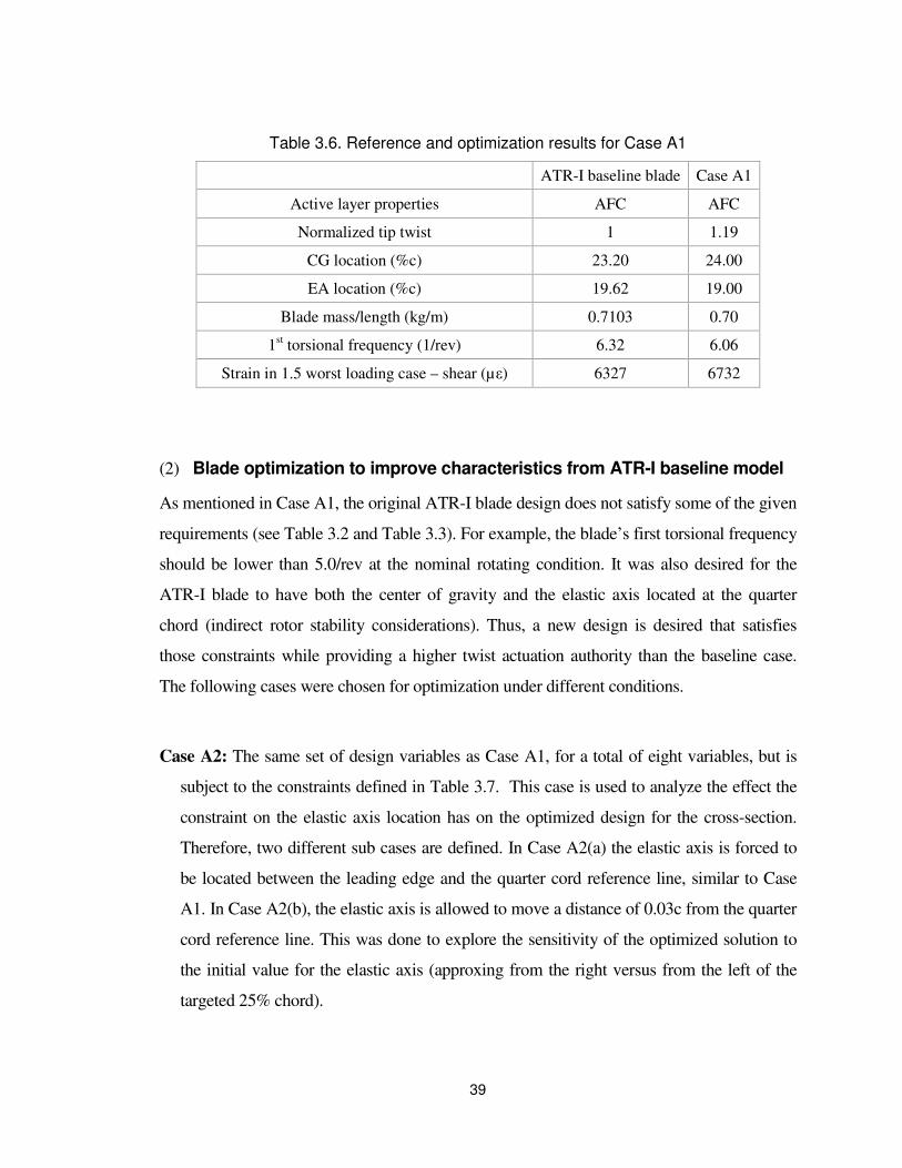
39

Table 3.6. Reference and optimization results for Case A1

ATR-I baseline blade Case A1

Active layer properties AFC AFC

Normalized tip twist 1 1.19

CG location (%c) 23.20 24.00

EA location (%c) 19.62 19.00

Blade mass/length (kg/m) 0.7103 0.70

1st torsional frequency (1/rev) 6.32 6.06

Strain in 1.5 worst loading case – shear (µε) 6327 6732

(2) Blade optimization to improve characteristics from ATR-I baseline model

As mentioned in Case A1, the original ATR-I blade design does not satisfy some of the given

requirements (see Table 3.2 and Table 3.3). For example, the blade’s first torsional frequency

should be lower than 5.0/rev at the nominal rotating condition. It was also desired for the

ATR-I blade to have both the center of gravity and the elastic axis located at the quarter

chord (indirect rotor stability considerations). Thus, a new design is desired that satisfies

those constraints while providing a higher twist actuation authority than the baseline case.

The following cases were chosen for optimization under different conditions.

Case A2: The same set of design variables as Case A1, for a total of eight variables, but is

subject to the constraints defined in Table 3.7. This case is used to analyze the effect the

constraint on the elastic axis location has on the optimized design for the cross-section.

Therefore, two different sub cases are defined. In Case A2(a) the elastic axis is forced to

be located between the leading edge and the quarter cord reference line, similar to Case

A1. In Case A2(b), the elastic axis is allowed to move a distance of 0.03c from the quarter

cord reference line. This was done to explore the sensitivity of the optimized solution to

the initial value for the elastic axis (approxing from the right versus from the left of the

targeted 25% chord).

40

Case A3: A Complete set of possible design variables for a section is used, totaling 29 design

variables1. The “ply-thickness” used here is actually the multiple of the nominal pre-preg

ply-thickness. Although the ply-thickness is a discrete value, which is a multiple of an

integer, it is considered a continuous value. Due to the optimization scheme used, all

design variables are treated as continuous.

Case A4: Only and all the 12 ply angles constitute the set of design variables. They are angle

of plies for outer E-glass, S-glass at nose, 1st AFC on top, 1st AFC on bottom, E-glass

between 1st top and bottom AFC plies at nose, 2nd AFC on top, 2nd AFC on bottom, E-

glass between 2nd top and bottom AFC plies at nose, web-extension on top, web-extension

on bottom, 1st spar-web rib, 2nd spar-web rib .

The new sets of constraints are shown in Table 3.7. Table 3.8 contains the initial values for

the different design variables used in each of these cases.

Table 3.7. Constraints for cases with characteristics improved from the ATR-I baseline case

Case A2(a) Case A2(b), Case A3 and Case A4


Elastic axis (EA) 0.17c < EA <

0.25c 0.22c < EA < 0.28c



Local Strain in the worst loading case

1.5xMax strain < ultimate strength of original constituent material


1 A given “layer” in the cross section corresponds to a ply of constant thickness (required from a finite-element

meshing point of view). Since a “layer” can be made of different materials each having their own ply angle, one

may have a larger number of design variables associated with ply angles than with ply thicknesses in a given

cross section.

41

Table 3.8. Initial design values of Case A2, A3 and A4

Case A2(a), (b) Case A3 Case A4

All ply-thickness 1.0 1.0 1.0

Ply Angles (degrees) N/A N/A [0 / 0 / +30 / -30 / +45 /

-30 / +30 / 0 /0 / 0 / 0 / 0]2

Active start 0.0456c 0.0456c 0.05c

Active end 0.85c 0.85c 0.85c

Web extension 0.05c 0.05c 0.05c

Ballast weight mass (0.186, 0.105) (0.186, 0.105) (0.1765, 0.0863)

Ballast weight location (0.022c, 0.85c) (0.022c, 0.85c) (0.0c, 0.918c)

Spar location 0.2c, 0.634c 0.634c 0.609c

Case A2

Figure 3.3(a) and Figure 3.4(a) show the convergence history of the normalized objective

function and the normalized blade parameters for Case A2(a) with the two different initial

values for the spar location of 0.2c and 0.634c, respectively. Similar to Figure 3.2, the shaded

area represents the feasible range of these parameters. The only constraint that is not within

the feasible range is the location of the elastic axis. The convergence history of the spar

location, the length of the web extension, the position of the front and rear ballast weights,

and the start/end of the active regions are shown as functions of the chord-wise position in

the airfoil in Figure 3.3(b) and Figure 3.4(b), and summarized in Table 3.9. Since the only

active constraint violated is the elastic axis location, the spar location is the most effective

variable that can be changed in order to place it within the feasible range.

For this Case A2(a), the final location of the spar depends on its initial value. By giving the

spar location an initial value (0.20c) close to its lower bound (0.10c), then its final position is

2 [outer E-glass, S-glass at nose/ 1st AFC on top/ 1st AFC on bottom/ E-glass between 1st top and bottom AFC

plies at nose/ 2nd AFC on top/ 2nd AFC on bottom/ E-glass between 2nd top and bottom AFC plies at nose/ web-

extension on top/ web-extension on bottom/ 1st spar-web rib/ 2nd spar-web rib]

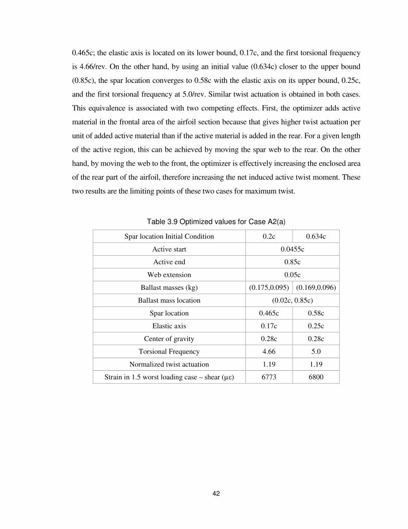
42

0.465c; the elastic axis is located on its lower bound, 0.17c, and the first torsional frequency

is 4.66/rev. On the other hand, by using an initial value (0.634c) closer to the upper bound

(0.85c), the spar location converges to 0.58c with the elastic axis on its upper bound, 0.25c,

and the first torsional frequency at 5.0/rev. Similar twist actuation is obtained in both cases.

This equivalence is associated with two competing effects. First, the optimizer adds active

material in the frontal area of the airfoil section because that gives higher twist actuation per

unit of added active material than if the active material is added in the rear. For a given length

of the active region, this can be achieved by moving the spar web to the rear. On the other

hand, by moving the web to the front, the optimizer is effectively increasing the enclosed area

of the rear part of the airfoil, therefore increasing the net induced active twist moment. These

two results are the limiting points of these two cases for maximum twist.

Table 3.9 Optimized values for Case A2(a)

Spar location Initial Condition 0.2c 0.634c


Active end 0.85c

Web extension 0.05c

Ballast masses (kg) (0.175,0.095) (0.169,0.096)

Ballast mass location (0.02c, 0.85c)

Spar location 0.465c 0.58c

Elastic axis 0.17c 0.25c

Center of gravity 0.28c 0.28c

Torsional Frequency 4.66 5.0

Normalized twist actuation 1.19 1.19

Strain in 1.5 worst loading case – shear (µε) 6773 6800

43

0 1

1.2

1.25

Obje

ctive f

unction


0 1-3

-2

-1

0

1

Norm

aliz

ed C

onstr

ain

ts

Iteration Number

loc CG

loc EA

Blade weight

Tor freq

Max strain

(a)

0 10

0.1

0.2

0.3

0.4

0.5

0.6

0.7

0.8

0.9

1

Iteration Number

Norm

aliz

ed location w

rt C

hord

length

(b)

Figure 3.3. Case A2(a) optimization history for initial spar location at 0.2c.

(a) Objective function convergence history (top) and normalized blade parameters (bottom), and corresponding (b) spar location (*), web extension (|), front and rear ballast weights (•), and start and end of active region (- x -), all normalized by chord length

44

0 1 2 3 41.19

1.195

1.2

1.205

Obje

ctive f

unction


0 1 2 3 4

0

1

2

3

Norm

aliz

ed C

onstr

ain

ts

Iteration Number

loc CG

loc EA

Blade weight

Tor freq

Max strain

(a)

0 1 2 3 40

0.1

0.2

0.3

0.4

0.5

0.6

0.7

0.8

0.9

1

Iteration Number

Norm

aliz

ed location w

rt C

hord

length

(b)

Figure 3.4. Case A2(a) optimization history for initial spar location at 0.634c.


45

Figure 3.5 and Figure 3.6 show the result for Case A2(b) with the same initial values for the

spar location as in Figure 3.3 and Figure 3.4, respectively. The optimized solution is

summarized in Table 3.10. In this Case A2(b), the spar location (0.635c), the location of the

elastic axis (0.28c), the torsional frequency (5.0 /rev), and the normalized twist actuation

(1.2) are not sensitive to the initial value of the spar location, unlike Case A2(a). The effect of

allowing the elastic axis move to the right of the quarter cord reference line is to allow the

spar to move further back toward the trailing edge. When comparing the optimized result for

Case A2(a) with an initial spar location at 0.634c and the solution for Case A2(b), it is

observed that the elastic axis location and torsional frequency have practically the same

values. Nevertheless, the twist actuation in Case A2(b) is slightly higher (1%) than in Case

A2(a). Moving the spar further toward the trailing edge, increases the amount of active

material placed on the front area of the cross-section, therefore an improvement in twist

actuation is obtained.

Table 3.10. Optimized values for Case A2(b) for both initial conditions of spar location


Active end 0.85c

Web extension 0.05c

Ballast masses (kg) 0.163, 0.099

Ballast mass location 0.001c, 0.868c

Spar location 0.635c

Elastic axis 0.28c

Center of gravity 0.28c

Torsional Frequency 5.0

Normalized twist actuation 1.2

Strain in 1.5 worst loading case – shear (µε) 6800

46

0 1 2 3

1.2

1.25

Obje

ctive f

unction


0 1 2 3-5

-4

-3

-2

-1

0

1

Norm

aliz

ed C

onstr

ain

ts

Iteration Number

loc CG

loc EA

Blade weight

Tor freq

Max strain

(a)

0 1 2 30

0.1

0.2

0.3

0.4

0.5

0.6

0.7

0.8

0.9

1

Iteration Number

Norm

aliz

ed location w

rt C

hord

length

(b)

Figure 3.5. Case A2(b) optimization history for initial spar location at 0.2c.


47

0 11.2005

1.201

1.2015

1.202

1.2025

Obje

ctive f

unction


0 1-1.5

-1

-0.5

0

0.5

1

Norm

aliz

ed C

onstr

ain

ts

Iteration Number

loc CG

loc EA

Blade weight

Tor freq

Max strain

(a)

0 10

0.1

0.2

0.3

0.4

0.5

0.6

0.7

0.8

0.9

1

Iteration Number

Norm

aliz

ed location w

rt C

hord

length

(b)

Figure 3.6. Case A2(b) optimization history for initial spar location at 0.634c. (a) Objective function convergence history (top) and normalized blade parameters (bottom), and

corresponding (b) spar location (*), web extension (|), front and rear ballast weights (•), and start and end of active region (- x -), all normalized by chord length

48

CASE A3

Figure 3.7 shows the convergence history of the normalized objective function and various

normalized blade parameters for Case A3, as well as the convergence history of the spar

location, the length of the web extension, the position of the front and rear ballast weights,

and the start/end of the active regions as functions of the chord-wise position in the airfoil.

The 1st torsional frequency was the most difficult variable to keep within the required bounds.

The optimal spar location ended up being set at 0.747c, and the active region extends to its

limits. Case A3 took 30 iterations to meet the convergence criteria. Although it seems to be

already converged around 15 iterations according to Figure 3.7, it is noticed that the variables

are still slightly changing in Figure 3.8, and one of the (maybe-too-tight) convergence criteria

took longer to be met.

Figure 3.8(a) shows the evolution of the ply-thicknesses over 30 iterations. The thickness of

the outer active composite ply increases to 78% above the nominal ply-thickness while that

of the outer and web E-glass plies decreases to half of the nominal ply-thickness. Since 0.5 is

a lower bound for the thickness design variable, this indicates that the optimizer is trying to

eliminate some of the plies in favor of others. Also, since the outer active plies have a bigger

effect in twist than the inner ones, even though both of these plies are increased over the

nominal thickness, the optimizer is allowing the outer ply to increase more than the inner one.

The increment in nominal thickness is bound by the blade mass/length constraint which

reaches its upper limit. Adding passive material on the nose region increases torsional

stiffness as well as twist actuation. Adding passive material on the active material region

results in a reduction of the twist actuation.

Figure 3.8(b) shows the ply angle variation during the optimization process. Although the set

of design variables includes all the ply angles, it only shows the ply angles of the active

material plies, the passive ply between active plies, and nose plies. Ply angles for outer E-

glass, web and web extension are not shown since they remained at 0o. Active ply angles

converge to [+49o/-52o] instead of ±45o, the ply angles for the active material that would

theoretically produce maximum twist actuation. The lack of sensitivity around the optimum

point at ±45o for the active plies does not allow the optimizer to reach that global minimum.

49

The ply angle for the nose moves to –9o and the spar moves to 0.747c, further back than in

Case A2(b). This decreases the stiffness and compensates for the material lost at the web,

and helps the elastic axis stay within the prescribed boundaries.

0 5 10 15 20 25 301.3

1.4

1.5

1.6

1.7

1.8

Obje

ctive f

unction


0 5 10 15 20 25 30-3

-2

-1

0

1

Norm

aliz

ed C

onstr

ain

ts

Iteration Number

loc CG

loc EA

Blade weight

Tor freq

Max strain

(a)

0 5 10 15 20 25 300

0.25

0.5

0.75

1

Iteration Number

Norm

aliz

ed location w

rt C

hord

length

(b)

Figure 3.7. Case A3 optimization history

(a) Objective function convergence history (top) and normalized blade parameters (bottom), and

corresponding (b) spar location (*), web extension (|), front and rear ballast weights (•), and

start and end of active region (- x -), all normalized by chord length

50

0 5 10 15 20 25 300

0.5

1

1.5

2

2.5

3

3.5

Iteration Number

Ply

thic

kness

outer E-glass

AFC 1

E-glass between AFC 1-2

AFC 2

inside E-glass

front web-wxt E-glass

rear web-ext E-glass

web 1

web 2

(a)

0 5 10 15 20 25 30

-100

-50

0

50

100

Iteration Number

Lam

ination a

ngle

nose E-glass

AFC 1-top & buttom

AFC 2-top & bottom


inside E-glass

(b)

Figure 3.8. Evolution of Case A3 (a) ply-thickness and (b) ply angles evolution

CASE A4

This case took 11 iterations to converge (Figure 3.9(a)); the normalized twist actuation

obtained is 31% higher than the baseline case. Similar to Case A2(b), but now with the

complete set of ply angles included among the design variables, Figure 3.9(b) shows the

convergence of ply angles for the active plies, the passive ply between active plies, and the

nose plies.

51

0 1 2 3 4 5 6 7 8 9 10 111.1

1.15

1.2

1.25

1.3

1.35

Obje

ctive f

unction


0 2 4 6 8 10 12-1.5

-1

-0.5

0

0.5

1

Norm

aliz

ed C

onstr

ain

ts

Iteration Number

loc CG

loc EA

Blade weight

Tor freq

Max strain

(a)

0 2 4 6 8 10 12

-100

-50

0

50

100

Iteration Number

Lam

ination a

ngle

nose E-glass

AFC 1-top & buttom

AFC 2-top & bottom


inside E-glass

(b)

Figure 3.9. Case A4 optimization history

(a) Objective function convergence history (top) and normalized blade parameters (bottom), and corresponding (b) Evolution of ply angles

52

The ply angle from the active material ply converges to approximately ± 45˚ as well. The

nose E-glass ply angle moves slightly away from 0˚ toward –9˚. These changes adjusted the

torsional stiffness of the blade (resulting 1st torsional frequency is 4.89/rev) and the elastic

axis location moved toward the leading edge to 0.252c. The final design does not show

higher active twist authority than Case A3, but it is still higher than Case A2.

(3) Comparison of ATR-I blade optimization cases

The results obtained by designing the cross section using the optimization framework are

summarized in Table 3.11. These cases demonstrate that even though the constraints are

tighter than in Case A1, better designs than the original ATR-I reference blade can still be

obtained. Case A2 shows that the new constraints can be accommodated by the same set of

design variables as in Case A1 and provides very similar twist actuation performance. Case

A3 showed the highest twist actuation authority. It can be expected since Case A3 has more

design variables than others, which translates into a larger design space. Even though Case

A3 presents the highest twist actuation, this optimum solution is not practical. The optimized

ply-thicknesses are not integer quantities. As explained previously, the ply-thicknesses

should be a multiple of the nominal ply-thickness. Allowing an adjustment on the ply angles

provided an extra 11% increase in the twist authority from Case A2.

Table 3.11. Optimized results for Cases 2, 3 and 4

Case A2(a) Case A3 Case A4

Tip twist (deg) 1.19 1.70 1.31

Spar location 0.58c 0.74c 0.60c

CG location (%c) 0.28c 0.28c 0.27c

EA location (%c) 0.25c 0.25c 0.25c

Blade mass/length (kg/m) 0.675 0.71 0.676

1st torsional frequency (1/rev) 4.66 5.0 4.83

Maximum strain - shear (µε) 6800 6628 6800

53

3.1.3 Summary of ATR-I design optimization

The developed framework is exemplified in the NASA/Army/MIT ATR-I blade case. The

examples showed that the twist performance of the original ATR-I blade, which was already

successfully manufactured and tested, could be enhanced to at least 20% higher actuation

performance when designed with the suggested optimization framework. During this

numerical study, the following six phenomena were noticed.

The constraint of the elastic axis position has an important effect on the position of the spar

web in the cross section. By allowing the elastic axis to be located between the quarter cord

and the trailing edge, the web would locate further back toward the trailing edge than if the

elastic axis is forced to be between the leading edge and the quarter chord point.

The maximum strain occurred near the point of discontinuity in the layup thickness between

the active region and the nose region in the cross section. However, adding a passive ply in

the nose reduced the stress concentration that arose from that discontinuity. By adding

passive material in the nose, the actuation authority of the blade increased.

Instead of using one single most critical component of the strains, it was better to have three

separate constraints associated with the maximum strain of two normal and one in-plane

shear components. This avoids discontinuity in the constraint, reducing the problem’s

nonlinear characteristics. Also, by considering three components, the resulting strain/stress

may be better distributed in the cross section.

As expected, including ply angles in the design variables made it more difficult for the

optimizer to converge than in the case in which the spar location, ballast masses and location,

web extension, and start and end position for the active material are used as design variables.

The optimization process was very sensitive to the initial values of the design variables. This

54

sensitivity was expected for the nonlinear nature of the problem and the gradient-based

optimization scheme. The optimizer converged much faster to a local optimum with a

feasible initial condition. As explained in Chapter 2 , ‘fmincon’ is used as an optimization

tool provided by MATLAB. It minimizes an objective function with a constrained nonlinear

multivariable problem. The problem of optimizing an active twist rotor is a nonlinear one and

solutions may fall at local minima. The testing cases showed this phenomenon actually is

observed, especially when the initial condition is not within the feasible region. The problem

here arises due to the complexity of this design; it is not easy to find the feasible initial

condition by changing design variables using experience derived from earlier designs. The

approach used here is to run the optimization cases for short iterations with these infeasible

initial points and find the feasible points through this optimization process. For future

reference, it may be worth to use an alternative optimization scheme that is not dependent on

the feasibility of the initial condition.

55

3.2 ATR-A blade design optimization

In this section, the developed methodology is applied to a more complex problem, the ATR-

A. It is given the designation as ATR-A since the blade geometry and properties are generally

representative of 21% scale model of the AH-64D Apache helicopter (Figure 3.10) blade.

Figure 3.10. Army AH-64 Apache helicopter DoD photo by Petty Officer 3rd Class Shawn Hussong, U.S. Navy. (Released)

This ATR-A example shows the framework’s ability to deal with a more complex model,

including different types of airfoil and the swept-droop-twist tip blade geometry. As

mentioned earlier, for the ATR-A, MFC has been introduced instead of AFC. MFC has

introduced integrated electrodes so the electric feed of the active plies can be implemented

inside the skin layup. In comparison with ATR-I, when AFCs were used and the electric feed

was constraint to run along the spar web, this new feature adds additional freedom to the

design space. To handle these complexities, additional steps are introduced beyond the

optimization itself. Besides the two nested optimization loops, special pre-processing of the

model and at the end, post-processing/analysis of the optimized design were introduced.

These steps address the added complexity of a modern blade and the demands of the

manufacturability of one’s design.

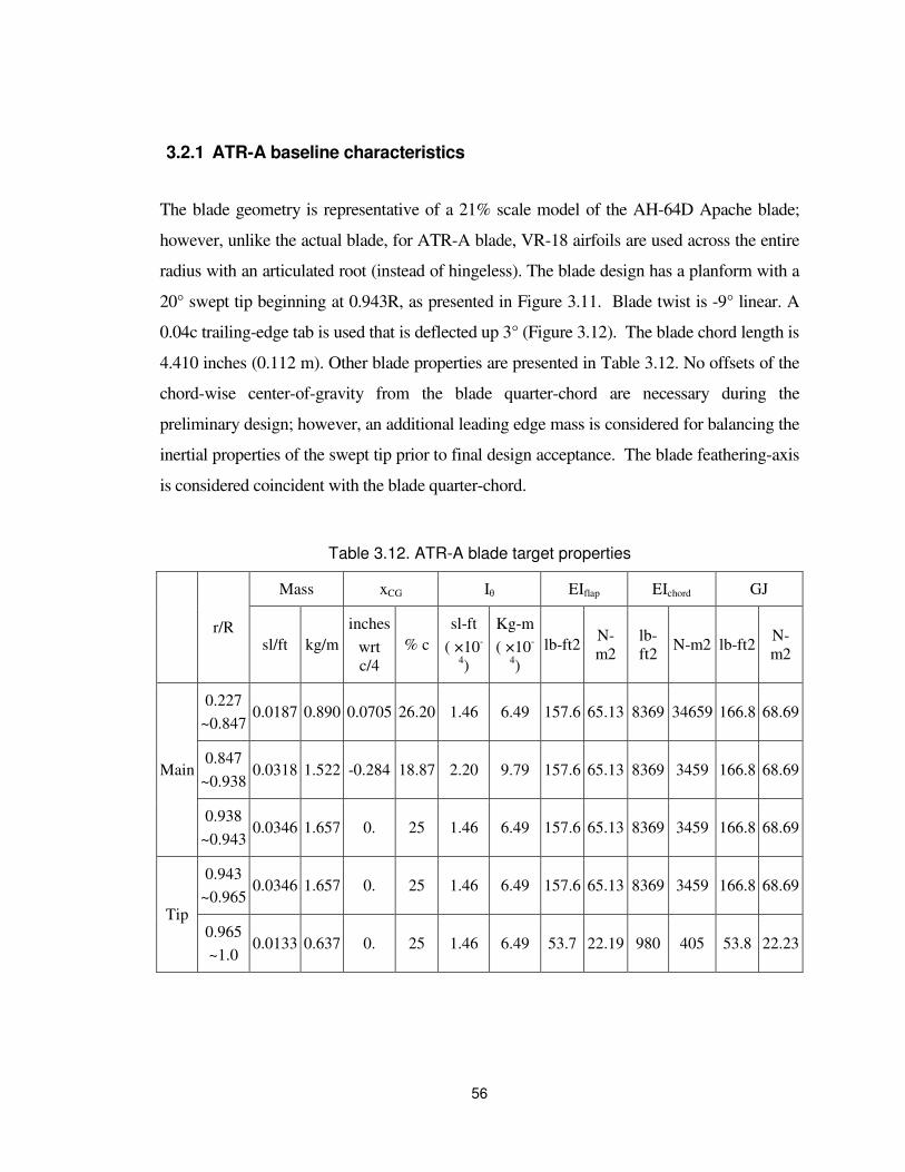
56

3.2.1 ATR-A baseline characteristics

The blade geometry is representative of a 21% scale model of the AH-64D Apache blade;

however, unlike the actual blade, for ATR-A blade, VR-18 airfoils are used across the entire

radius with an articulated root (instead of hingeless). The blade design has a planform with a

20° swept tip beginning at 0.943R, as presented in Figure 3.11. Blade twist is -9° linear. A

0.04c trailing-edge tab is used that is deflected up 3° (Figure 3.12). The blade chord length is

4.410 inches (0.112 m). Other blade properties are presented in Table 3.12. No offsets of the

chord-wise center-of-gravity from the blade quarter-chord are necessary during the

preliminary design; however, an additional leading edge mass is considered for balancing the

inertial properties of the swept tip prior to final design acceptance. The blade feathering-axis

is considered coincident with the blade quarter-chord.

Table 3.12. ATR-A blade target properties

r/R

Mass xCG Iθ EIflap EIchord GJ

sl/ft kg/m

inches

wrt c/4

% c

sl-ft

( ×10-

4)

Kg-m

( ×10-

4)

lb-ft2 N-m2

lb-ft2

N-m2 lb-ft2 N-m2

Main

0.227

~0.847 0.0187 0.890 0.0705 26.20 1.46 6.49 157.6 65.13 8369 34659 166.8 68.69

0.847

~0.938 0.0318 1.522 -0.284 18.87 2.20 9.79 157.6 65.13 8369 3459 166.8 68.69

0.938

~0.943 0.0346 1.657 0. 25 1.46 6.49 157.6 65.13 8369 3459 166.8 68.69

Tip

0.943

~0.965 0.0346 1.657 0. 25 1.46 6.49 157.6 65.13 8369 3459 166.8 68.69

0.965

~1.0 0.0133 0.637 0. 25 1.46 6.49 53.7 22.19 980 405 53.8 22.23

57

Figure 3.11. ATR-A model blade planform (R = 60.48 inches. Not to scale.)

Figure 3.12. ATR-A Cross sectional view (VR18 with trailing edge tab)

For the ATR-A, Macro-Fiber Composite (MFC) actuators are placed from approximately

0.227R to 0.943R, with R = 60.48 inches (1.536 m). The stiffness and mass characteristics,

initially used for the optimization studies are set as follows:

130 lb-ft2 ≤ EIFlap ≤ 160 lb-ft2

5450 lb-ft2 ≤ EILag ≤ 6600 lb-ft2

135 lb-ft2 ≤ GJ ≤ 160 lb-ft2

0.0165 sl/ft ≤ m ≤ 0.0185 sl/ft

0.13 -ft ≤ Iθ ≤ 0.00016 sl-ft

Extent of MFCs 0.9430.227 1.0

20°

4.41 in

4.691 in

58

3.2.2 Pre-processing: Needs and adjustments

(1) Mesh generator

Before starting on the full optimization process, the capabilities and limitations of the cross-

section mesh generation need to be re-visited base on the additional geometric complexities

of this case.

The finite element mesh for the composite plies is generated automatically with the code

developed by Brown (Brown 2003). It creates the mesh based on geometric parameters such

as the aspect ratio of elements, chord length, and nominal thickness of plies. It has great

versatility; however, it also comes with some limitations. Since the code is already quite

complex, revising it is not desirable. Instead, a series of steps to find ways to solve the

limitations with the current code is proposed and described below. Some of the changes to

overcome the limitations are done prior and/or outside the optimization cycle as adjusted

designs, while other changes are integrated in the optimization process as new subroutines.

For the first case, the limitations are studied and an adjusted design is suggested to model the

blade as close as possible. The effect of the adjusted model is compared with respect to the

original one. When the effect is negligible, that design is considered throughout the process

as an alternative model.

For the others, new subroutines to accommodate the changes were developed using

MATLAB, and they were integrated in the optimization process along with the mesh-

generator. These additions adjust some details on the modeling of the cross section that the

mesh-generator is not able to change automatically. This approach is different from the one

above since it happens within the code and make the design follows the model more closely,

rather than accepting small difference between the model and the design. This approach also

accommodates the changes without revising the mesh-generation itself as mentioned.

59

When applied to the optimization of more complex blade cross sections, five main limitations

have been identified in generating the finite element mesh:

• Mesh overlapping

• Trailing edge tab modeling

• Element distortion

• Electrode modeling

• Foam implementation

In the following sections, these limitations and the approach to work around them are

presented in more detail. Among those five limitations, the mesh overlapping, the element

distortion, and the foam implementation uses the first approach to overcome the limitations,

and the rest follows the second approach.

Mesh Overlapping

Even though the mesh generator is very versatile, in some cases it creates overlapped meshes

that cause the UM/VABS to crash. This code failure usually involves overlapping at the nose

(leading edge) region of the cross section when the innermost ply becomes thicker than

double its nominal thickness (Figure 3.13).

The proposed approach is to introduce a small ply discontinuity at the edge of the nose where

the overlapping occurs as shown in Figure 3.14. Analysis on example cases, one with

discontinuity and one without, has been performed. When stiffness and inertia constants are

compared, the change in the solution is negligible, indicating that the results are similar

enough to allow the discontinuity without affecting the results of the optimization. Thus by

using this approach, further code modification is not required.

60

Figure 3.13. Element overlapping close-up

Figure 3.14. Discontinuity introduction at nose

Trailing edge tab modeling

The mesh-generator cannot accurately model the trailing edge of the ATR-A cross section

which has a tab. The ATR-A cross section is based on the VR-018 airfoil, which has a

trailing edge tab with a slope of 3°. To capture this feature within the code, the elements are

re-generated for the trailing edge tab based on elements that the current mesh-generator

produces. When the nodes at the start of the trailing edge and at the tip are given, a midpoint

between them is generated. Based on these three points along the chord, new elements for the

trailing-edge tab are generated that can capture the reflex tab in airfoils like the VR-18.

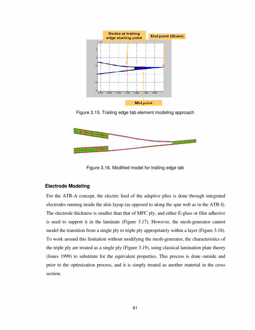
61

Figure 3.15. Trailing edge tab element modeling approach

Figure 3.16. Modified model for trailing edge tab

Electrode Modeling

For the ATR-A concept, the electric feed of the adaptive plies is done through integrated

electrodes running inside the skin layup (as opposed to along the spar web as in the ATR-I).

The electrode thickness is smaller than that of MFC ply, and either E-glass or film adhesive

is used to support it in the laminate (Figure 3.17). However, the mesh-generator cannot

model the transition from a single ply to triple ply appropriately within a layer (Figure 3.18).

To work around this limitation without modifying the mesh-generator, the characteristics of

the triple ply are treated as a single ply (Figure 3.19), using classical lamination plate theory

(Jones 1999) to substitute for the equivalent properties. This process is done outside and

prior to the optimization process, and it is simply treated as another material in the cross

section.

62

Figure 3.17. MFC unit electrode layup

Figure 3.18. Inappropriate transition modeling

Figure 3.19. Single ply model for electrode (pink)

63

Distorted element

Another problem in the process of generating the mesh was the appearance of that unwanted

triangular elements were observed at the beginning of the upper active plies. The mesh-

generator is attempting to create a quadrilateral element, but because it makes the initial and

last node coincident, it results in a triangle (Figure 3.20). The effect of this triangular element

has been studied by comparing the case with triangular element and the case with that

element modified.

Figure 3.20. Distorted quad element from mesh generator

First, an optimization was run with triangular elements in the mesh. Then the triangular

elements were changed to quadrilateral ones using by PATRAN (Figure 3.21)

(MSCSoftware 2004), and the changed input file was fed to the optimizer for one cycle.

Comparison of this result with the unchanged element model led to the conclusion that the

presence of the triangular elements does not affect the solution and leaving the eventual

element there is acceptable.

64

Figure 3.21. Corrected quad element by PATRAN

Foam implementation

The actual ATR-A blade has foam inside, which the mesh-generating code was not able to

model. Changing the mesh generator to model the foam was beyond the scope of this study.

But, since the foam could be added externally by using MSC.PATRAN, a study was

conducted to assess its effect in the optimum design.

This analysis was performed as follows: (1) a complete optimization case was run; (2) the

final UM/VABS file obtained from the optimization code was loaded in MSC.PATRAN,

since UM/VABS’s input file is compatible with MSC.NASTRAN file; (3) a mesh was

created to included foam in the entire cross section; and (4) the file from MSC.PATRAN was

loaded into the optimization code and a simple analysis (without iteration) was run to obtain

new values of a affected blade properties, constraints, and objective function.

Figure 3.22 shows a case with one type of foam used for the entire cross section (E=36.0

MPa, υ=0.26, and ρ=35 kg/m3) and the mesh elements on the nose region of the blade.

Table 3.13 shows the results of this analysis. It is observed that including the foam changes

several properties save for the center of gravity location. For the type of foam included in this

case, a significant change is observed in the location of the elastic axis: it moves from 0.255c

65

to 0.3342c (31.1%) and the 1st torsional frequency increases by 22.8%. The actuation angle

and blade weight slightly increase by 2.8% and 3.4%, respectively. These relative changes

were shown to be relatively constant for a given airfoil shape. From these results, changing

the constraints for the location of the elastic axis and the 1st torsional frequency during the

optimization process may be required, so when the foam is included the final value is within

the required limits. In this way one indirectly takes into account the foam effects without

having to model it during the optimization.

0.025 0.02 0.01

5

0

5

(a) (b)

Figure 3.22. Nose cross section mesh

(a) Without foam, and (b) With foam after modified in MSC.PATRAN.

Table 3.13.Effects of unmodeled foam in the design of the active cross section

Without foam With foam

Tip twist actuation (deg peak-to-peak) 3.57 3.67 (2.8%)

Blade mass / length (kg/m) 0.790 0.817 (3.4%)

Center of gravity (CG) 0.255c 0.255c

Elastic axis (EA) 0.255c 0.334 (31.1%)

1st torsional frequency (1/rev) 4.71 5.77 (22.5%)

66

(2) Initial design adjustment

At the very beginning, most of the design variables were selected based on the ATR-I blade.

Although the blades are not the same, that provided an initial cross-sectional design for the

brand new case. At this stage, the worst loading cases were also based on the ATR-I blade.

Then several inner-loop analyses/optimization runs were performed and the variables and/or

constraints also manually adjusted to find a more reasonable and feasible initial design. In

spite of the problem being highly nonlinear, there are some variables whose effects on the

blade characteristics are less difficult to anticipate. For example, the effect of the ballast mass

and location to the center of gravity and the blade mass is straighfoward. On the other hand,

the start location of the active region affects the maximum strain while the spar location

moves the elastic axis—something not obvious. Once the initial design is adjusted and

selected, the design is sent to the outer loop. Then the aeroelastic analysis is performed based

on that design, and the worst loading is updated.

3.2.3 ATR-A blade optimization cases

The objective of this section is to study the application of the proposed optimization process

to the more complex ATR-A rotor. The goal is to maximize the twist actuation while keeping

the airfoil, ply-thickness and ply angles fixed. The constraints are set to ensure the blade

design is a feasible solution, as summarized in Table 3.14. The seven design variables are the

spar location, the magnitude and the location of two ballast masses, and the start/end of the

active regions. Eight different cases are studied to find the best configurations and further

study the effects of the parameters. The case descriptions are shown in Table 3.15. These

seven design variables and their initial values, corresponding to the ATR-A baseline blade,

are presented for each case in what follows.

Regarding the elastic axis, from the earlier studies discussed in section 3.2.2(1)0, it is known

that the foam will move the elastic axis backward. Anticipating that, the elastic axis

constraint is confined between 0.10c and 0.20c. After foam implementation, the elastic axis is

67

expected to move to near 0.25c, which is the desired location. The center of gravity is

constrained between 0.20c and 0.26c, near the desired 0.25c. The maximum strain constraint

is defined for each material for both normal and shear components. For example, the

maximum shear strain of the MFC is given at 5500 µε, which usually is the most critical

constraint. Thus, any MFC layer would not experience a shear strain higher than 3670 µε,

which would be 5500 µε considering the safety factor of 1.5.

Table 3.14. Constraints used for the ATR-A optimization study

Elastic axis (EA) 0.10c < EA< 0.20c




Local Strain in the worst loading case

1.5xMax strain < ultimate strength of original constituent material

Ballast weight (kg/m) 0.0 <weight < 1.0

Active region 0.085 c< Loc<0.85c


During the optimization process, the following effects are noticed. As the spar location

moves backward, the twist rate becomes higher since it increases the active region forward of

the spar location. However, the change in the spar location also pushes the elastic axis

backwards. To reduce the maximum shear strain, the starting location of the active region

needs to go backwards to the upper bound, which will reduce the twist rate. Moving the end

location of the active region backward increases the twist rate, but this does not have as much

of an effect as moving the start of the active region forward. Unlike the ATR-I blade, a 45o

lamination angle of passive ply between two active plies at the nose increases the shear strain.

Blade weight and center of gravity constraints are preventing the active end from moving

further backwards, which would increase the twist rate. From this, it is noticed once more

that the optimization of active twist rotors is a very nonlinear and complex problem.

68

Based on these studies and the given requirements, the following cases were chosen and each

studied through the optimization process. For all these cases, the nose reinforcement was

introduced instead of the D-spar-like reinforcement used in ATR-I.

Table 3.15. ATR-A optimization cases

No. of

web plies

No. of extra

plies at nose

Upper limit

of spar location

Case T1(a)

3

3 0.85

Case T1(b) 5 0.85

Case T1(c) 3 0.45

Case T1(d) 5 0.45

Case T2(a)

2

3 0.85

Case T2(b) 5 0.85

Case T2(c) 3 0.45

Case T2(d) 5 0.45

69

CASE T1(a)

The goal for this case is to generate the initial (feasible) design that will be used for the other

seven variants to follow. For this first case, the following conditions were applied:

� Design variables: Active start, active end, two ballast weights, spar location

� End of the nose reinforcement = Active start +0.1c

� Three plies are used for the nose reinforcement

� Three plies are used on the spar-web

Table 3.16. Case T1(a) Initial and optimized values

Initial Optimized

Active start 0.131c 0.170c

Active end 0.762c 0.767c

Ballast weight mass (0.284, 0.00) (0.310, 0.0000)

Ballast weight location (0.022c, 0.576c) (0.022c, 0.477c)


Twist rate (deg/m) 2.70 2.27


Blade mass / length (kg/m) 0.850 0.870

Max strain (µm/m) 6180 5500


Elastic axis (EA) 0.257c 0.200c

Table 3.16 shows the critical blade characteristics related to the design variables and the

constraints of the initial and the optimized designs. Figure 3.23 presents the optimization

history of the objective function, active tip twist, and the normalized constraints (a), as well

as the corresponding results for each iteration (b).

The initial design has violated two constraints: the location of the elastic axis and the

maximum strain, which are shown in Figure 3.23(a) and in bold in the first column of Table

3.16. As a result, the spar location moved forward to satisfy the elastic axis constraint (shown

in italic in the second column of Table 3.16). For maximum strain constraint violation, the

start location of the active region moved backward, which decreased the active twist rate to

2.27 from 2.70, about 20%.

70

(a)

(b)

Figure 3.23. Case T1(a) Optimization history

(a) Objective function convergence history (top) and normalized blade parameters (bottom), corresponding (b) spar location (*), web extension (|), front and rear ballast weights (•), and start and end of active region (- x -), all normalized by chord length.

71

CASE T1(b)

Consider the follow characteristics of this case:


� End of the nose reinforcement= Active start +0.1c

� Five plies are used for the nose reinforcement


Table 3.17. Case T1(b) Initial and optimized values

Initial Optimized










Center of Gravity (CG) 0.260c 0.260c


As studied earlier, the optimization scheme used here showed better performance when the

initial design was a feasible one. When the initial design was not feasible, the code

sometimes crashed or took a longer to converge to the optimal solution. To help loosen the

maximum strain constraint violation of the initial design of Case T1(a), additional plies are

applied to the nose reinforcement (5 plies). This also helped move the elastic axis forward.

By reducing the violated constraints, the optimization only took two iterations to converge.

As a result, the active twist rate decreased from 2.67 to 2.53, about 5.6%. This shows that the

constraints can be satisfied, mostly by moving the spar location backward, without sacrificing

the active twist rate significantly as when the start of the active region was moved backward

as shown in Case T1(a).

72

(a)

(b)

Figure 3.24. Case T1(b) Optimization history (a) Objective function convergence history (top) and normalized blade parameters (bottom), corresponding (b) spar location (*), web extension (|), front and rear ballast weights (•), and start and end of active region (- x -), all normalized by chord length.

73

CASE T1(c)

Another variant of Case T1(a) is considered here with the following characteristics:


� End of the nose reinforcement= Active start +0.1c



� Upper limit and initial point of spar location are now reduced to 0.45c

Table 3.18. Case T1(c) Initial and optimized values

Initial Optimized









Max strain 6150 5490



Similar to Case T1(b), one of the initial values that violates the constraints, in this case the

elastic axis, was moved to a feasible point. To help loosen the elastic axis constraint violation

at the initial design of Case T1(a), the upper limit and the initial location of the spar web were

set to 0.45c. This located the initial elastic axis within the constraint but the maximum strain

out of bound. To avoid this violation, the start location of the active region was backward

and, as a result, the active twist rate has been reduced. This case also took only two iterations

to converge.

74

(a)

(b)

Figure 3.25. Case T1(c) Optimization history (a) Objective function convergence history (top) and normalized blade parameters (bottom), corresponding (b) spar location (*), web extension (|), front and rear ballast weights (•), and start and end of active region (- x -), all normalized by chord length.

75

CASE T1(d)

Finally, the following is considered:



� Five plies are used for nose reinforcement



Table 3.19. Case T1(d) Initial and optimized values

Initial Optimized












This is a combination of Case T1(b), which has five plied at the nose reinforcement, and Case

T1(c),which has a spar location at 0.45c, and there is no constraint violated at the initial point.

The optimum design did not move far from the initial design and the active twist rate

increased slightly to 2.470 from 2.455.

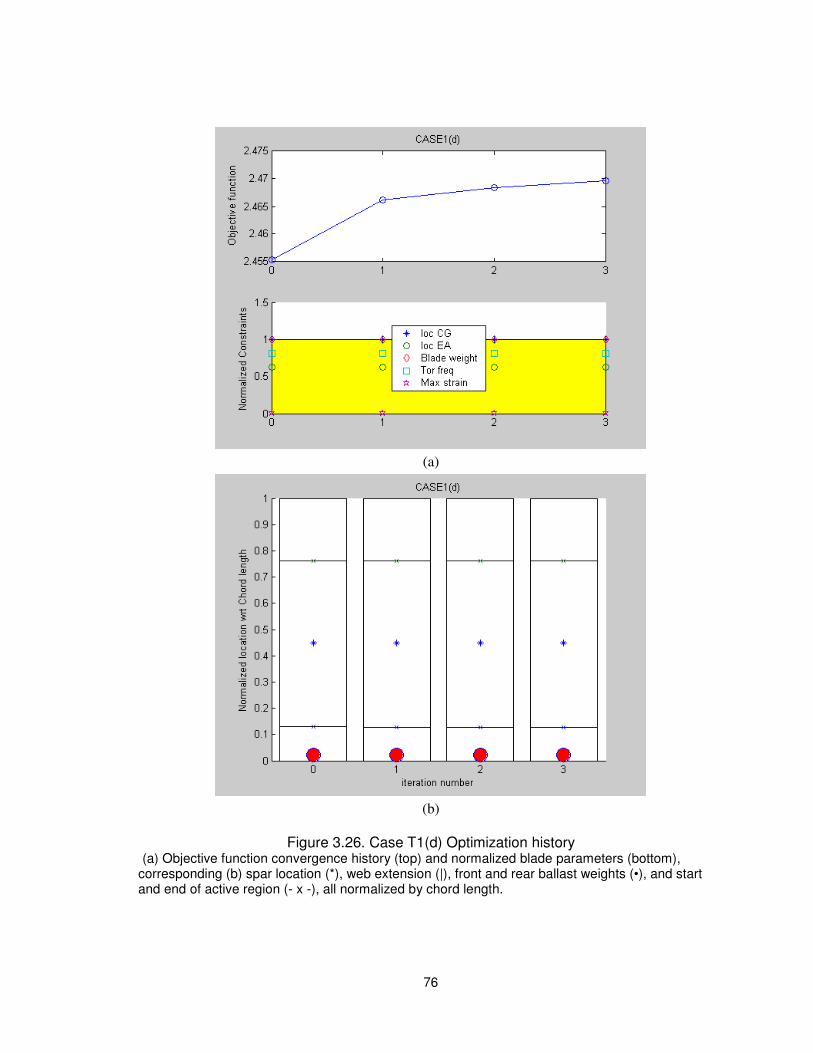
76

(a)

(b)

Figure 3.26. Case T1(d) Optimization history


77

CASE T2(a)

This is a modified case from Case T1(a). This case serves as a baseline for the other variants

of Case T2 to follow. For this second baseline case, the following conditions were applied:



� Nose reinforcement with triple the thickness

� Two plies are used on the spar-web

Table 3.20. Case T2(a) Initial and optimized values

Initial Optimized












Here the plies on the spar-web have been reduced from three to two. It moves the elastic axis

closer to the feasible range of the constraint by reducing the stiffness, but not enough to move

into the feasible range. Adversely, this made the maximum strain constraint worse. As a

result, when optimized, the start point of the active region moved backward to satisfy the

maximum strain constraint. Moreover, the final active twist rate is 2.37, which is 4.4%

greater than Case T1(a), 2.27, while all constraints are satisfied.

78

(a)

(b)

Figure 3.27. Case T2(a) Optimization history


79

CASE T2(b)

Consider the following:



� Five plies are used for the nose reinforcement


Table 3.21. Case T2(b) Initial and optimized values

Initial Optimized












This is a combination of Case T1(b) and Case T2(a). As in Case T1(b), two more plies are

added to the nose reinforcement to meet the maximum strain constraint violation at the initial

design of Case T2(a). This also helps to move the elastic axis forward to 0.2002c but slightly

out of the upper limit, 0.20c. The optimization history shows a small “bump”, but mostly the

variables remain near their initial values and the elastic axis constraint is now satisfied.

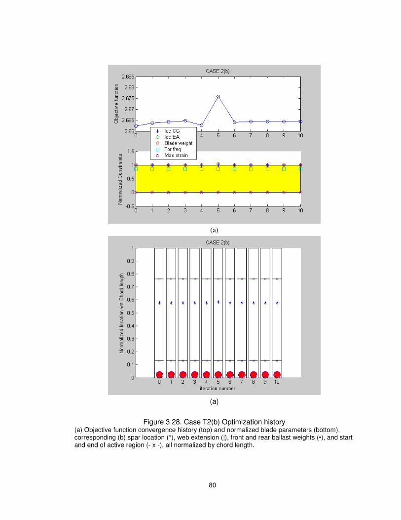
80

(a)

(a)

Figure 3.28. Case T2(b) Optimization history


81

CASE T2(c)







Table 3.22. Case T2(c) Initial and optimized values

Initial Optimized












This case modifies Case T2(a) similarly as it was done Case T1(c). This case has two plies

for the spar-web as in Case T2(a). As in Case T1(c), the upper limit and the initial location of

the spar are set to 0.45c. At the initial design, the elastic axis is moved to a feasible point and

the maximum strain is outside of its upper limit. Similar trends are noticed in Case T1(c). The

start location of the active region was moved backward and, as a result, the active twist rate

was reduced by 19.5%.

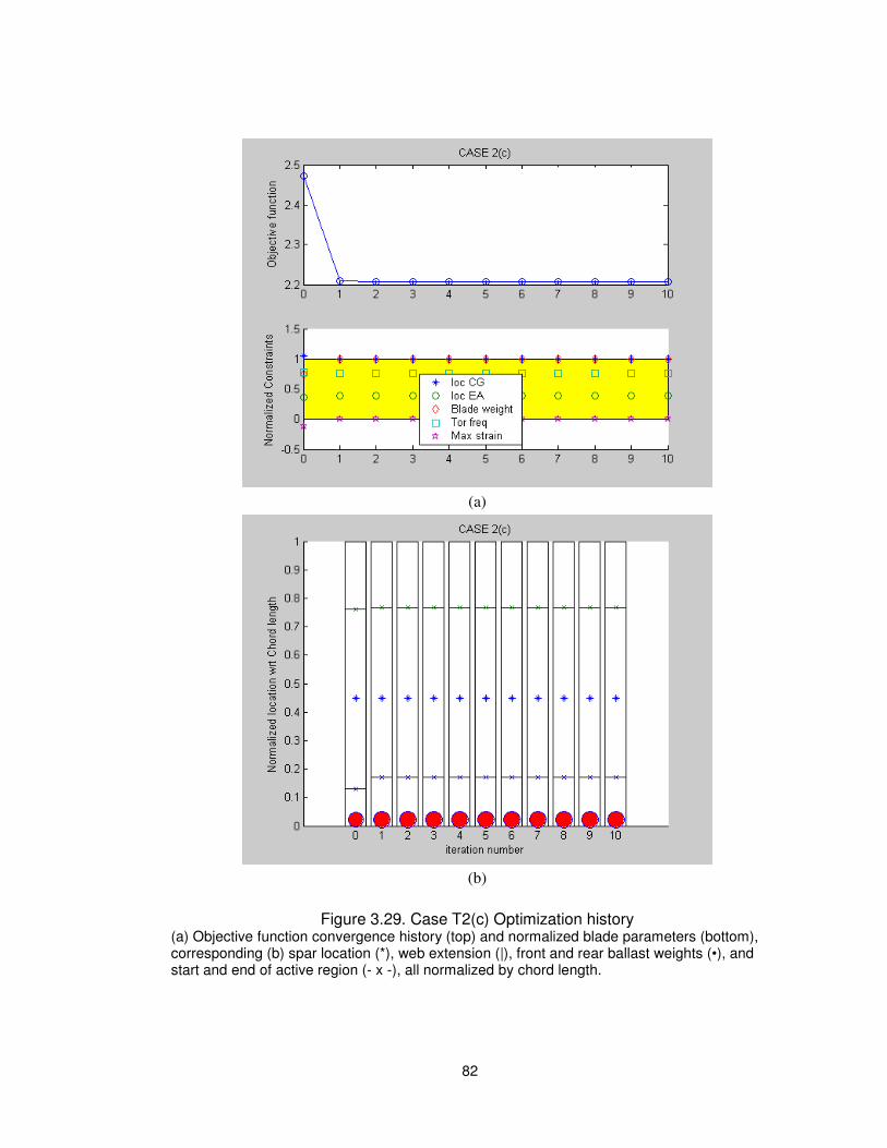
82

(a)

(b)

Figure 3.29. Case T2(c) Optimization history


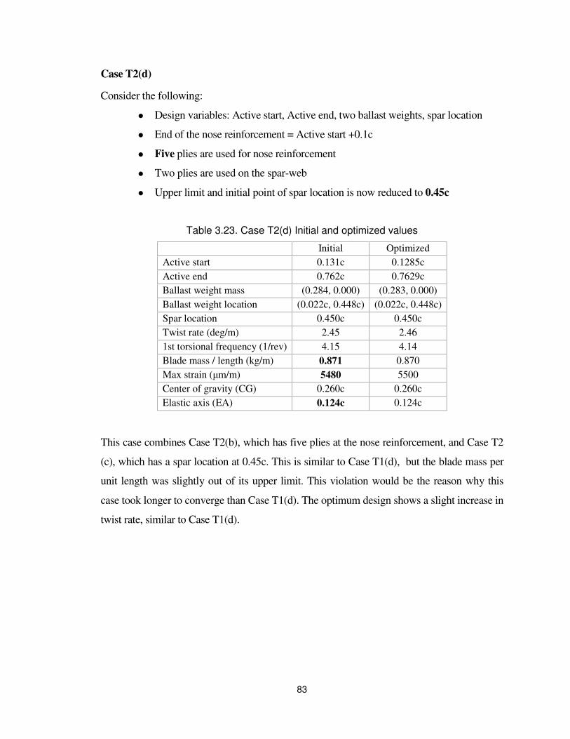
83

Case T2(d)


� Design variables: Active start, Active end, two ballast weights, spar location


� Five plies are used for nose reinforcement


� Upper limit and initial point of spar location is now reduced to 0.45c

Table 3.23. Case T2(d) Initial and optimized values

Initial Optimized












This case combines Case T2(b), which has five plies at the nose reinforcement, and Case T2

(c), which has a spar location at 0.45c. This is similar to Case T1(d), but the blade mass per

unit length was slightly out of its upper limit. This violation would be the reason why this

case took longer to converge than Case T1(d). The optimum design shows a slight increase in

twist rate, similar to Case T1(d).

84

(a)

(b)

Figure 3.30. Case T2(d) Optimization history


85

3.2.4 Comparison of the various ATR-A optimized cases and down selection

As presented in the previous section 3.2.3, there were 8 cases chosen for which optimized

solution were found. A summary of them is presented in Table 3.24.

Table 3.24. ATR-A case study summary

No. of

web plies

No. of extra

plies at nose

Upper limit

of spar location

Active twist rate

(deg/m)

Active tip

twist angle (deg)

Case T1(a)

3

3 0.85c 2.27 2.61

Case T1(b) 5 0.85c 2.52 2.91

Case T1(c) 3 0.45c 2.21 2.55

Case T1(d) 5 0.45c 2.47 2.85

Case T2(a)

2

3 0.85c 2.37 2.73

Case T2(b) 5 0.85c 2.66 3.07

Case T2(c) 3 0.45c 2.21 2.54

Case T2(d) 5 0.45c 2.46 2.84

Tip twist angle = twist rate * length of active region

Length of active region (m)= 1.1523 = 1.609*(0.943-0.227)

Among those cases, Case T1(b) and Case T2(b) are selected as the recommended ones for

further consideration. Those cases show the maximum twist rate at a given number of web

plies. Figure 3.31and Figure 3.32 show the cross sectional view for each case.

The filling foam is then implemented in both of these cases. The distorted quad element is

fixed in PATRAN, as described in the previous section. As expected, the elastic axis has

moved backwards and has ended up near the quarter chord, as summarized in Table 3.26 and

Table 3.27. The material properties of the foam are presented in Table 3.25.

86

(a)

(b)

Figure 3.31. Case T1(b) Cross section layup

(a)whole cross section (b) near end of nose reinforcement and spar location

(a)

(b)

Figure 3.32. Case T2(b) Cross section layup

(a)whole cross section (b) near end of nose reinforcement and spar location

Table 3.25. Material Properties of the foam

E (MPa) υ ρ (kg/m3)

35 0.26 35

87

Table 3.26. Case T1(b) before and after the inclusion of foam

Foam implementation No Yes












Table 3.27. Case T2(b) before and after the inclusion of foam

Foam implementation No Yes












88

3.2.5 Analysis of effect of span-wise design optimization

In this section, the effect of the span-wise design optimization is explored. The cross-

sectional layups are designed differently along the blade. The blade is divided into four

sections along the span. The first three sections may have active materials while the last

section is the passive tip. For the ATR-A cases, the spacial distributions is as follows:

• Section 1: 0.227R to 0.4657R (Active region)



• Section 4: 0.943R to 1.000R

In each of the sections, a set of design variables are independently defined. Considering

manufacturability of the blade, the spar location for each section is set to the same value,

which implies in linking the corresponding design variables in each section to a unique one.

The remaining design variables are:

• Section 1: active start, active end, ballast weight (2)



• Section 4: active start, active end, ballast weight (2), spar location

Constraints and bounds are shown in Table 3.28. They are the same as used for Case T1(b)

for each section, except the lower bound of the active region. Sections 2, 3 and 4 have the

lower bound of the active region set to 0.0455c instead of 0.846c, which may provide larger

twist actuation. The cross sectional layup is also the same as in Case T1(b). Only section 4,

the tip region, has E-glass 0/90 instead of MFC.

89

Table 3.28. Constraints and bounds for the span-wise optimization case

Elastic Axis (EA) 0.10c < EA< 0.20c

Center of Gravity (CG) 0.20c < CG < 0.26c



Local Strain in the worst case loading 1.5xMax strain < ultimate strength of



Active region 0.084615c (0.0455c) < Loc<0.85c


Table 3.29. Initial and optimized values for the span-wise optimization case

Initial Optimized

Tip twist angle (deg) 3.37 3.43


Table 3.30. Optimized length of the MFC for the different active sections

Upper Lower

Section 1 (mm) 75.0 73.4

Section 2 (mm) 79.0 77.2

Section 3 (mm) 80.6 78.1

Figure 3.34 shows the optimization history of the objective function and constraints. The

initial and optimized values of tip twist angle and first torsional frequencies are presented in

Table 3.29. Table 3.30 shows the optimized length of the MFC on each active section.

Table 3.31 shows the initial and optimized values for each section, while Figure 3.33 presents

the summary of the cross sectional designs at different blade sections.

90

(a) Section 1 (b) Section 2

(c) Section 3 (d) Section 4

Figure 3.33 Span-wise optimization history – cross sectional design

Spar location (*), web extension (|), front and rear ballast weights (�), and start and end of active

region (- x -), all normalized by chord length.

For this particular design, the additional freedom brought up by span-wise design variables

had only a small impact in the objective function (~2% increase in tip twist) and a small

adjustment in the constraints (see

Table 3.31). This came with the additional complexity/cost due to the different actuator sizes

required for each section (Table 3.30). The trade is not worthwhile for ATR-A and the design

will continue without the subdivision of the active region of the blade.

91

(a)

(b)

Figure 3.34. Span-wise Optimization history

(a) Objective function convergence history (b) normalized constraints (*: location of CG, O: location of EA, �: blade weight, �: max strain, �: torsional frequency) (Red: section 1, Blue: section 2, Green: section 3, Magenta: section 4)

92

Table 3.31. Initial and optimized values of the span-wise optimization case

SEC Parameters Initial Optimized

1

Active start

Active end

Ballast weight mass


Spar location

Blade mass / length (kg/m)

Center of gravity (CG)

Elastic axis (EA)

Max strain (µstrain)

0.085c

0.740c

0.290, 0.000

0.060c, 0.459c

0.463c

0.870

0.260c

0.172c

5810

0.085c

0.740c

0.290, 0.000

0.060c, 0.501c

0.505c

0.8700

0.2600c

0.200c

5810

2

Active start

Active end

Ballast weight mass


Spar location



Elastic axis (EA)


0.052c

0.742c

0.284, 0.000

0.060c, 0.459c

0.463c

0.870

0.260c

0.172c

5480

0.052c

0.741c

0.284, 0.000

0.060c, 0.501c

0.505c

0.870

0.260c

0.200c

5500

3

Active start

Active end

Ballast weight mass


Spar location



Elastic axis (EA)


0.046c

0.742c

0.282, 0.00

0.060c, 0.459c

0.463c

0.870

0.260c

0.171c

5000

0.046c

0.742c

0.282, 0.000

0.060c, 0.501c

0.505c

0.870

0.260c

0.200c

5012

4

Active start(passive material)

Active end(passive material)

Ballast weight mass


Spar location



Elastic axis (EA)


0.100c

0.804c

0.401, 0.000

0.060c, 0.589c

0.463c

0.915

0.252c

0.161c

1280

0.090c

0.823c

0.385, 0.099

0.060c, 0.501c

0.505c

0.870

0.257c

0.192c

1220

93

3.2.6 Refined ATR-A blade optimum design

(1) Update worst-case loading with previous optimum design

Outer Loop

As mentioned earlier, the aerodynamic load analysis is not included within the optimization

loop and is only updated once a converged solution if obtained in the optimization loop

(Figure 2.2). Among the optimization cases above, Case T1(b) has been chosen as an

optimized design and sent to the outer loop. The aeroelastic analysis was performed on this

design, Case T1(b), using CAMRAD II (analysis performed at NASA LaRC/ US Army

VTD).

The aeroelastic loadings are provided at every 15˚ azimuthal angle on every given station

along the blade for unactuated case and 3P actuated case at 45˚ phase angle. Then the critical

load for all six load components is selected by scanning the loads for all azimuthal angles, all

radial positions along the blade, and all flight conditions. Figure 3.35 shows an example of

the actuated loads associated with the torsional moment 3P, 45 phase angle. The point where

the torsional load is maximium is identified: 0.23R and 120˚ angle, and the other five

components corresponding to the same point are collected as part of the worst case loading

matrix.

Based on the new loads calculated from CAMRAD II with the optimized result of Case

T1(b), new maximum load cases were obtained, as exemplified in Table 3.32. In each matrix,

the first row represents the loads for the maximum torsion case; the second the maximum for

flap-wise bending moment; the third the maximum for lag-wise bending moment; the forth

the maximum for axial force; the fifth the maximum for chord-wise shear force; and the sixth

the maximum for normal shear force. Maximum loads at other blade locations were also

computed and are shown in Appendix 4.

94

Figure 3.35. Torsional moment at 3P actuated, 45 phase angle

95

Table 3.32. Updated worst-case loading with optimized design

Max loads for Torsion case (in - lb) 0.1R 0.2R 0.3R 0.4R 0.5R 0.6R 0.7R 0.8R 0.9R 1.0R

-78.4 -77.8 -82.8 -78.4 -73.1 -66.9 -58.9 -49.8 -42.2 0.0

14.4 12.3 29.1 19.6 18.5 -30.3 -2.4 -3.9 5.2 0.0

-14.0 -13.1 14.7 15.0 -5.6 -4.0 -2.6 -1.0 2.0 0.0

-39.5 -38.5 -18.3 -60.1 -55.2 -49.0 -41.0 -15.4 -7.1 0.0

-5.5 -5.0 12.1 -18.0 -5.9 15.6 7.6 3.4 2.6 0.0

-29.4 14.9 9.4 -1.0 -18.9 19.4 16.8 -24.9 2.3 0.0

Max loads for Flap-wise bending case (in -lb) 0.1R 0.2R 0.3R 0.4R 0.5R 0.6R 0.7R 0.8R 0.9R 1.0R

-15.0 -39.8 7.0 10.5 13.9 18.3 23.7 23.3 9.8 0.0

-63.6 -99.6 -60.7 -52.1 -48.9 56.0 80.0 92.8 34.6 0.0

1.3 -18.8 -34.3 -35.4 -26.3 -11.8 8.3 28.0 8.1 0.0

7.4 -12.4 -19.7 9.3 26.5 49.2 66.0 86.5 31.7 0.0

1.2 -34.3 -39.9 -16.1 -2.0 -13.7 34.8 65.1 24.7 0.0

7.1 -98.3 -50.3 1.8 21.3 -8.2 28.7 -6.5 33.9 0.0

Max loads for Lag-wise bending case (in - lb) 0.1R 0.2R 0.3R 0.4R 0.5R 0.6R 0.7R 0.8R 0.9R 1.0R

343.5 113.0 84.2 81.4 61.5 48.5 40.4 41.1 32.8 0.0

123.5 -130.0 -49.8 80.2 70.9 40.1 2.0 -10.5 20.2 0.0

510.9 306.5 313.6 317.3 282.7 232.3 169.0 102.5 45.8 0.0

452.3 241.4 244.7 -2.3 -20.5 -23.9 -13.9 -3.3 17.4 0.0

363.9 88.4 40.9 15.5 -22.4 228.3 -54.0 -18.3 9.7 0.0

505.0 -150.8 -124.3 128.8 -48.6 1.5 -4.4 18.4 15.7 0.0

Max loads for axial shear force case (lb) 0.1R 0.2R 0.3R 0.4R 0.5R 0.6R 0.7R 0.8R 0.9R 1.0R

1394.9 1319.9 1261.6 1182.0 1079.7 954.6 806.8 634.4 436.6 0.0

1337.8 1266.8 1214.2 1146.2 1066.5 955.7 810.2 640.2 444.9 0.0

1400.1 1323.1 1262.4 1180.2 1077.4 949.7 800.0 628.6 435.8 0.0

1404.0 1327.8 1267.8 1187.7 1086.2 961.6 813.9 642.7 447.6 0.0

1381.0 1305.5 1247.4 1136.7 1039.3 947.1 778.3 613.8 424.8 0.0

1402.0 1260.9 1205.9 1178.0 1080.7 925.2 782.0 621.5 445.8 0.0

Max loads for chord shear force case (lb) 0.1R 0.2R 0.3R 0.4R 0.5R 0.6R 0.7R 0.8R 0.9R 1.0R

23.5 16.7 3.9 1.9 0.2 -1.2 -2.2 -2.1 -0.8 0.0

21.5 12.4 3.6 3.2 1.3 -1.8 -3.7 -7.9 -5.8 0.0

17.0 12.1 1.0 2.4 4.1 6.1 7.2 6.0 3.1 0.0

17.8 12.8 1.5 2.3 -0.5 -3.2 -5.3 -6.9 -6.5 0.0

30.2 21.9 7.7 -6.0 -5.2 6.5 -7.8 -9.3 -9.1 0.0

16.9 8.9 -2.6 1.1 -0.8 -0.8 -2.7 -5.2 -7.3 0.0

Max loads for normal shear force case (lb) 0.1R 0.2R 0.3R 0.4R 0.5R 0.6R 0.7R 0.8R 0.9R 1.0R

-6.4 2.7 0.4 -1.4 -0.3 -0.9 -0.4 -1.9 -8.6 0.0

-0.1 10.4 1.6 0.7 -0.4 1.4 3.5 -2.4 -18.1 0.0

-11.6 -4.8 -1.1 0.9 1.7 2.4 3.5 0.7 -9.2 0.0

-7.9 -3.7 -0.2 0.4 2.4 1.6 1.2 -2.4 -17.3 0.0

-5.1 -2.7 -1.6 0.6 2.4 2.6 4.9 1.1 -16.1 0.0

-11.8 11.4 2.6 2.7 3.7 4.7 7.0 -3.6 -18.5 0.0

96

Inner Loop

Then the optimization was run again with a layup similar to Case T1(b) (Figure 3.31) but

with updated loads as in Table 3.32. Constraints and design variables are kept the same as

Case T1(b) and are shown on Table 3.33 for completeness. This case will be known as Case

Tu. The initial and optimized values are presented in Table 3.34. shows the optimized layup

sketch of this case, while Figure 3.36 shows the optimization history. Since the initial values

used on the optimization process were the optimized solution for Case T1(b), only a few

iterations were needed in order to reach convergence. The results of the application of the

new loads on the design show that the MFC plies move toward the leading edge from

0.1296c to 0.1051c, which produces an increment in the active tip twist angle of 6.5% (3.10˚

instead of 2.91˚). This is due to a slight decrease of the design loads, which have been used as

the worst loading from the previous iteration.

Table 3.33.Constraints and bounds for Case Tu

Elastic axis (EA) 0.10c < EA< 0.20c




Local Strain in the worst loading case 1.5×Max strain < ultimate strength of



Active region 0.084615 c< Loc<0.85c


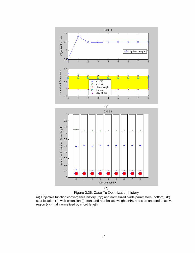
97

(a)

(b)

Figure 3.36. Case Tu Optimization history

(a) Objective function convergence history (top) and normalized blade parameters (bottom); (b) spar location (*), web extension (|), front and rear ballast weights (�), and start and end of active region (- x -), all normalized by chord length.

98

Figure 3.37. Optimized Layup result for Case Tu

Table 3.34. Case Tu Initial and optimized results

Initial Optimized

Active start 0.127c 0.105c (-19%)

Active end 0.761c 0.737c (-3%)



Spar location 0.491c 0.505

Tip twist angle (deg) 2.91 3.10 (6.5%)



Max strain 5100 5500

Center of gravity (CG) 0.272c 0.260c (-4.5%)


99

(2) Analysis of the effect of using stiffer foam

The effect of placing stiffer foam on the D-spar region of the cross section is studied in this

section. Properties of different foam placed on the cross section are presented in Table 3.35.

Different cases were run based on the Case Tu layup shown in Figure 3.37, and they are

summarized in Table 3.36. Rohacell 31 IG and 71 IG are foam used on ATR-I on the fairing

region of the cross section. The value of υ is not given by the manufacturer. The

manufacturer provides E and G and assuming an isotropic material the value of υ was

computed. Case Tu1 represents a section with both regions of the cross section having the

same foam (Rohacell 31 IG.) Case Tu2 presents the same foam distribution used in ATR-I,

and in Case Tu3 much stiffer and denser foam is used on the D-spar section (Rohacell 200

WF.) In all the cases, the new set of loads presented in the first section of this report is used.

Table 3.35. Mechanical properties of foam

Commercial name E (MPa) G (MPa) υ ρ (kg/m3)

Rohacell 31 IG 36.0 13.0 0.385 32.0

Rohacell 71 IG 81.2 29 0.400 75.0

Rohacell 200 WF 350 150 0.167 205

Table 3.36. Cases analyzed in foam study

D-spar fairing

Case Tu1 31 IG 31 IG

Case Tu2 71 IG 31 IG

Case Tu3 200 WF 31 IG

The results for Case Tu1 are presented in Table 3.37. When light foam is used in both regions

of a cross section it is observed that actuation only increased 1% from 3.1o to 3.13o, while

also a slight reduction in max shear strain value is obtained. The CG is slightly moved aft

(2%) while the EA is changed by 42% toward the back of the airfoil, locating it around 0.28c.

100

Table 3.37. Comparison with foam implementation for Case Tu1

without foam with foam






Tip twist angle (deg) 3.10 3.13 (1%)

1st torsional frequency (1/rev)

4.44 4.46 (0.5%)


Max strain (µε) 5500 5430 (-1.3%)

Longitudinal strain (µε) 2600 2290 (-11%)

Lateral strain (µε) 2530 2200 (-13%)

Shear strain (µε) 5500 5430 (-1%)

Center of gravity (CG) 0.260c 0.265c (2%)

Elastic axis (EA) 0.200c 0.283c (42 %)

For Case Tu2 and Case Tu3, an initial optimized result was obtained with a lower value for

the blade weight upper bound value (0.84 and 0.80 kg/m respectively), such that, when the

foam is implemented, the weight upper limit is not violated. All other constraints were kept at

their original values (Table 3.34). By reducing the upper bound of the blade mass per unit

length, a reduction on the twist actuation is observed. This reduction comes as a consequence

of the reduction on the length of the active ply to compensate for the reduction of ballast

weight all in order to keep the center of gravity position constant.

Results for Case Tu2 are presented in Table 3.38. Increasing the density of the foam placed

on the D-spar region produces an increase of twist actuation of 1% and at the same time the

maximum shear strain is reduced by 2% from 5500 to 5390µε. The first torsional frequency

changes from 4.47 to 5.35 /rev (20%). The center of gravity is changed from 0.260c to 0.267c

(3%), while the elastic axis moves from 0.200c to 0.279c (39%).

101







Spar location 0.504 0.504

Tip twist angle (deg) 3.09 3.10 (1%)

1st torsional frequency (1/rev) 4.47 5.35 (20%)


Max strain (µε) 5500 5390 (-2%)



Shear strain (µε) 5500 5390 (-2%)

Center of gravity (CG) 0.260c 0.265c (2%)

Elastic axis (EA) 0.200c 0.279c (39%)

The comparison between Case Tu1 and Case Tu2 shows that the effect on the variables is

similar with the exception of the first torsional frequency, which for Case Tu2 increased by

20% while in Case Tu1 is not significantly altered.

The results for Case Tu3 are presented in Table 3.39. Even though using stiffer and denser

foam on the D-spar region slightly reduces the actuation by 1%, it has a significant effect on

the maximum strain reducing it from 5500 to 5120µε. Similar to Case Tu2, the first torsional

frequency increases from 4.52 to 5.54 /rev. The center of gravity is changed by 3% (from

0.260c to 0.267c) while the elastic axis moves from 0.200c to 0.300c (50%).

This analysis shows that placing denser and stiffer foam on the D-spar region of the cross

section helps to reduce the strain generated on the cross section without significantly

affecting the actuation obtained. Independent of the density of the foam, the location of the

CG is not affected, while the elastic axis changes at around 50% (approximately 0.2c to

0.3c). The density of the foam may affect the value of the first torsional frequency up to 20%.

102

Since using Rohacell 200WF provides a significant reduction in strain (between 7% and

12%) and a reduction on the ballast weight needed in the leading edge without a significant

effect on twist actuation (-1%), Case Tu3 is selected and considered further. For this case, the

length of the MFC plies with active fiber on it is 57.0 mm and 58.3 mm for the upper and

lower portion of the airfoil, respectively.







Spar location 0.500 0.500

Tip twist angle(deg) 3.07 3.03 (-1%)

1st torsional frequency (1/rev) 4.52 5.54 (23%)

Blade mass / length (kg/m) 0.800 0.906 (13%)

Max strain (µε) 5500 5120 (-7%)



Shear strain (µε) 5500 5120 (-7%)

Center of gravity (c) 0.260 0.267 (3%)

Elastic axis (c) 0.200 0.299 (50%)

Table 3.40 presents properties of all three cases when the foams are included accordingly.

Among these, Case Tu2 is selected since it has relatively higher tip twist angle with lower

maximum strain and the elastic axis is nearer to the quarter chord. Moreover, it is using the

materials that has heritages from ATR-I blade.

103

Table 3.40. Comparison of with foam implementation cases

Case Tu1

With foam

Case Tu2

With foam

Case Tu3

With foam

Active start 0.1051c 0.1048c 0.1038c

Active end 0.7373c 0.7265c 0.7088c

Ballast weight mass (0.295, 0.0) (0.274, 0.0) (0.248, 0.0)

Ballast weight location (0.06c, 0.501c) (0.06c, 0.499c) (0.06c, 0.496c)

Spar location 0.505c 0.504 0.500

Tip twist angle (deg) 3.13 3.10 3.03

1st torsional frequency (1/rev) 4.46 5.35 5.54

Blade mass / length (kg/m) 0.894 0.888 0.906

Max strain (µε) 5430 5390 5120

Longitudinal strain (µε) 2290 2300 2330

Lateral strain (µε) 2200 2200 2260

Shear strain (µε) 5430 5390 5120

Center of gravity (CG) 0.265c 0.265c 0.267

Elastic axis (EA) 0.283c 0.279c 0.299

3.2.7 Ballast mass

Figure 3.38 shows a schematic cross sectional view of two ballast mass implementations. For

Case Tu3, a ballast weight of 0.2475 kg/m is needed at the leading edge of the airfoil.

Tungsten is usually introduced as the material for the ballast mass. The density of tungsten is

19.3 kg/m3.

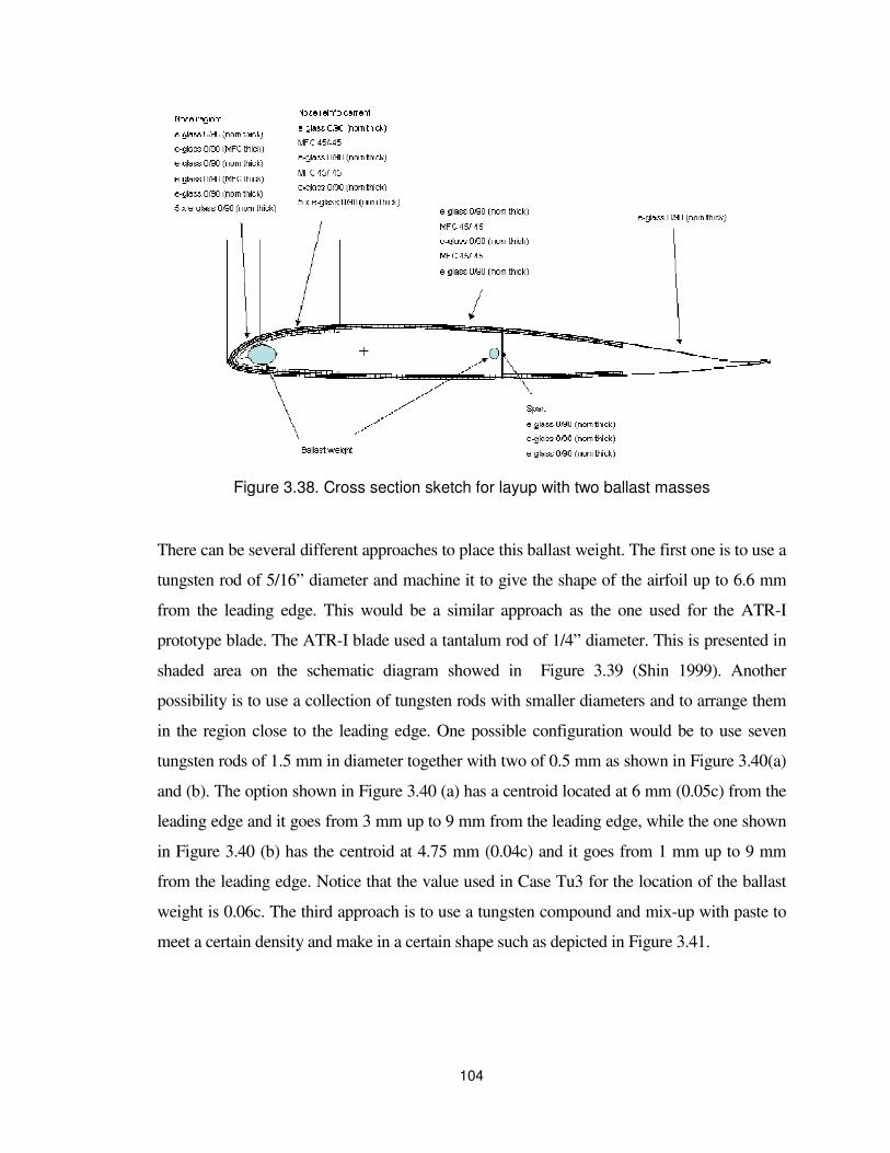
104

Figure 3.38. Cross section sketch for layup with two ballast masses

There can be several different approaches to place this ballast weight. The first one is to use a

tungsten rod of 5/16” diameter and machine it to give the shape of the airfoil up to 6.6 mm

from the leading edge. This would be a similar approach as the one used for the ATR-I

prototype blade. The ATR-I blade used a tantalum rod of 1/4” diameter. This is presented in

shaded area on the schematic diagram showed in Figure 3.39 (Shin 1999). Another

possibility is to use a collection of tungsten rods with smaller diameters and to arrange them

in the region close to the leading edge. One possible configuration would be to use seven

tungsten rods of 1.5 mm in diameter together with two of 0.5 mm as shown in Figure 3.40(a)

and (b). The option shown in Figure 3.40 (a) has a centroid located at 6 mm (0.05c) from the

leading edge and it goes from 3 mm up to 9 mm from the leading edge, while the one shown

in Figure 3.40 (b) has the centroid at 4.75 mm (0.04c) and it goes from 1 mm up to 9 mm

from the leading edge. Notice that the value used in Case Tu3 for the location of the ballast

weight is 0.06c. The third approach is to use a tungsten compound and mix-up with paste to

meet a certain density and make in a certain shape such as depicted in Figure 3.41.

105

Figure 3.39 Schematic diagram of the ATR-I blade design (Shin 1999)

(a) (b)

Figure 3.40. Position of ballast rods on leading edge of airfoil

Figure 3.41. Possible geometry of ballast mass

106

3.2.8 Strain Analysis

The strain analysis on the proposed design after the optimization indicated that the maximum

torsional strain occurs on the one-ply fairing and the web. To alleviate that, adjustments to

the optimized case are introduced as in Table 3.41 and the effects of the changed constraints

and the objective function are studied.

• CASE S1: Original ATR-A baseline

• CASE S2: Additional two Glass/Epoxy plies added to the web (butt ending).

• CASE S3: Extension of innermost 0/90 Glass/Epoxy ply from the active region

going all the way to the end of the fairing.

• CASE S4: Combination of CASE S2 and CASE S3.

Table 3.41. Case description

CASE S1 CASE S2 CASE S3 CASE S4

Thickness of spar (mm) 0.114× 3 0.114× 5 0.114× 3 0.114× 3

Thickness of the TE (mm) 0.114× 1 0.114× 1 0.114× 2 0.114× 2

Strain analysis on torsional strain per unit torque was performed to find the maximum strain

points. Table 3.42 shows the common properties for these cases. CASE S1 serves the

baseline for comparison of other cases. Table 3.55 in section 3.2.9 shows the detailed values

for CASE S1, which is the baseline for comparison of other cases. The results are

summarized in Table 3.43, Table 3.44 and Table 3.45. Figure 3.42 through Figure 3.45

present the distribution of the strain due to the unit torque application. The hot spots in CASE

S1 (baseline) were the one-ply fairing (35 µε/in-lb) and the web (27 µε/in-lb). CASE S2

reduces the fairing strain by 7% and the web by 26%. CASE 3 reduces the fairing strain by

14% and the web by 10%. CASE S4 reduces the fairing strain by 18.5% and the web by

22%. Adding the trailing edge (fairing) ply (CASE S3) reduces the twist actuation by ~2%

while adding plies to the web (CASE S2) improves the actuation (in this case, ~0.5%). The

combined modifications (CASE S4) present a reduction of ~1% from the baseline CASE S1.

107

For all cases, the center of gravity is basically unaffected. It moved aft but on the order of 3%

from the original position, or 0.8% chord. The elastic axis is the variable affected most. It

moved ~8% of its original value aft (or 2.25% of chord). Small changes are noticed on

frequencies but nothing was significant. Then, the biggest negative impact is associated with

the elastic axis position. Actuation is basically unaffected (Table 3.45) and the torsional strain

per unit torque is reduced at the hot spots (Table 3.44). Though the adjustment reduced the

strain at hot spots, by adding the plies to the web or the trailing edge, there also showed some

negative effects in mass per unit length and the location of the elastic axis. Since the hot spots

in the CASE S1 still satisfies the strain allowable, that case, which is the original ATR-A

baseline is kept as a final model.

Table 3.42. Common properties for sections 0, 1 & 2

Thickness of nose part (outer, inner) (mm) 0.114× (3, 3)

Thickness of nose reinforcement

(before, after active start) (mm) 0.114× (4, 5)

Space around ballast weight (mm) 0.114× 3

Active start (upper, bottom) (0.092c, 0.092c)

Active end (upper, bottom) (0.609c, 0.610c)

Electrode start(upper, bottom) (0.609c, 0.610c)

Electrode end (upper, bottom) (0.709c, 0.710c)

End of nose reinforcement 0.1920c

Spar location 0.5040

Table 3.43. Cross sectional properties (with foam)

Section


Mass CG loc

EA loc

Mass CG loc

EA loc

Mass CG loc

EA loc

Mass CG loc

EA loc

[kg/m] [%c] [%c] [kg/m] [%c] [%c] [kg/m] [%c] [%c] [kg/m] [%c] [%c]

0 0.227~0.847R 0.88 25.60 28.50 0.88 25.70 30.15 0.89 26.29 29.33 0.89 26.38 30.74

1 0.847~0.938R 1.50 19.38 28.50 1.51 19.45 30.15 1.51 19.83 29.33 1.52 19.89 30.74

2 0.938~0.943R 1.63 25.12 28.50 1.63 25.17 30.15 1.64 25.50 29.33 1.64 25.55 30.74

108

Table 3.44. Strain values for worst case loads


Thickness of spar (mm) 0.114× 3 0.114× 5 0.114× 3 0.114× 3

Thickness of the TE (mm) 0.114× 1 0.114× 1 0.114× 2 0.114× 2

Max strain (µε) 5160 5150 5170 5160

Longitudinal strain (µε) 2200 2170 2080 2050

Lateral strain (µε) 1930 1920 1910 1910

Shear strain (µε) 5160 5150 5170 5160

Table 3.45. Blade actuation properties


Thickness of spar (mm) 0.114 × 3 0.114× 5 0.114× 3 0.114× 3

Thickness of the TE (mm) 0.114 × 1 0.114× 1 0.114× 2 0.114× 2

Tip twist angle (deg) 3.05 3.07 3.00 3.01

-0.02 0 0.02 0.04 0.06 0.08

-0.04

-0.03

-0.02

-0.01

0

0.01

0.02

0.03

0.04

strain x 1.e12 /lb-in

-10

-8

-6

-4

-2

0

2

4

6

8

x 107

Figure 3.42. Case S1 Sectional distribution of strain due to unit torque (Γ12 per in-lbf)

109

-0.02 0 0.02 0.04 0.06 0.08

-0.04

-0.03

-0.02

-0.01

0

0.01

0.02

0.03

0.04

Case 2

strain x 1.e12 /lb-in

-8

-6

-4

-2

0

2

4

6

8

x 107



110


3.2.9 Refining the ATR-A Design

In this section, the study focused on the refinement of Case Tu2 to account for practical

manufacturing limitations and its impact on the cross section properties of the active blade.

Properties of the baseline materials and the commercially available materials are shown in

Table 3.47 and Table 3.46, respectively. The study resulted in a small adjustment to the cross

sectional parameters.

Table 3.46. Commercially available material properties provided by manufacturer

E-Glass Graphite IM7 Rohacell 31 IG Rohacell 71 IG

Remark Resin (F-155) Root/Resin (SP 381) Fairing D-spar

Weave Fabric Uni-tape

Thickness (mm) 0.12 0.14 - -

Density (kg/m3) 1716 1550 32 75

E11 (GPa) 20.7 165 0.036 0.092

E22 (GPa) 20.7 8.3 - -

ν12 0.13 0.34 0.385 0.04

G12 (GPa) 4.1 4.3 0.013 0.029

111

Table 3.47. Baseline material properties

MFC E-Glass

Graphite

IM7

(root)

Kapton Electrode

model

Rohacell

31 IG

Rohacell

71 IG

Remark Resin

F-155

Resin

SP 381 Fairing D-spar

Weave - Fabric Uni-tape

Thickness

(mm) 0.315 0.114 0.1397 - 0.315 - -

Density

(kg/m3) 4480 1716 1550 1100 1531 32 75

E11 (GPa) 20.0 19.3 142 1.0 0.036 0.0812

E22 (GPa) 12.3 19.3 8.3 1.0 - -

ν12 0.291 0.148 0.34 0.3 0.385 0.04

G12 (GPa) 3.78 4.1 4.9 0.7 0.013 0.029

d11 (m/V) 3 3.9×1010 - - - - - -

d12 (m/V) -1.9×1010 - - - - - -

telect (mm) 0.43 - - - - - -

Q11 (GPa) 21.10 19.73 1.10 14.14

Q12 (GPa) 3.78 2.92 3.30 2.14

Q22 (GPa) 12.98 19.73 1.10 14.14

Q33 (GPa) 3.78 4.10 0.70 3.10

Xt (µstrain) 3000 15000 15000 10000 10000 10000 10000

Yt (µstrain) 3000 10000 10000 10000 10000 10000 10000

S (µstrain) 3000 10000 10000 10000 10000 10000 10000

Xc (µstrain) 3000 10000 10000 10000 10000 10000 10000

Yc (µstrain) 5500 10000 10000 10000 10000 10000 10000

(1) Main blade layup

The main blade layup is shown in Figure 3.46. Figure 3.47 is a close up of the layup near the

ballast rod and presents how the additional mass would be integrated to the nose region. The

cross sectional constants for this case (with and without foam) are presented in Table 3.49.

3 Computed at aprox. 1250 V peak -to-peak to produce 1100 µstrain peak-to-peak

112

Table 3.49 also compares those properties with the cases when the material properties are

adjusted with commercially available ones. After the foam is included, the ballast weight is

increased to move the CG forward without violating the blade weight constraint. Table 3.48

presents the geometric properties of the active layer. The adjusted design has virtually the

same active tip twist as Case Tu2. The mass and stiffness matrices as well as the actuation

vector (SI units) are shown in Appendix 5.

Figure 3.46. Active cross section for Case Tu2 showing layup definition

Figure 3.47. Detail of the cross section near the ballast mass location

(Green: outer nose part, Pink: inner nose part, Grey: nose reinforcement before active region, Yellow: nose reinforcement after active region, Blue circle: tungsten rod, Red circle: E-glass

cover)

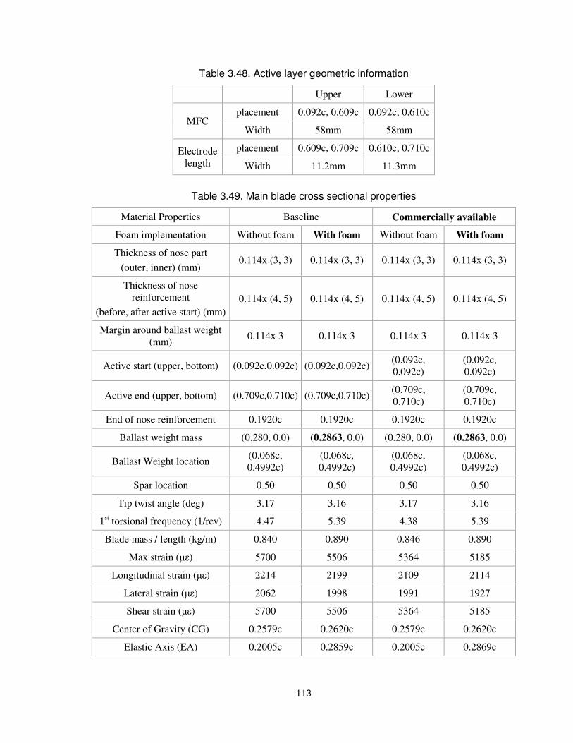
113

Table 3.48. Active layer geometric information

Upper Lower

MFC placement 0.092c, 0.609c 0.092c, 0.610c

Width 58mm 58mm

Electrode length

placement 0.609c, 0.709c 0.610c, 0.710c

Width 11.2mm 11.3mm

Table 3.49. Main blade cross sectional properties

Material Properties Baseline Commercially available

Foam implementation Without foam With foam Without foam With foam

Thickness of nose part

(outer, inner) (mm) 0.114x (3, 3) 0.114x (3, 3) 0.114x (3, 3) 0.114x (3, 3)

Thickness of nose reinforcement

(before, after active start) (mm)

0.114x (4, 5) 0.114x (4, 5) 0.114x (4, 5) 0.114x (4, 5)

Margin around ballast weight (mm)

0.114x 3 0.114x 3 0.114x 3 0.114x 3

Active start (upper, bottom) (0.092c,0.092c) (0.092c,0.092c) (0.092c, 0.092c)

(0.092c, 0.092c)

Active end (upper, bottom) (0.709c,0.710c) (0.709c,0.710c) (0.709c, 0.710c)

(0.709c, 0.710c)

End of nose reinforcement 0.1920c 0.1920c 0.1920c 0.1920c

Ballast weight mass (0.280, 0.0) (0.2863, 0.0) (0.280, 0.0) (0.2863, 0.0)

Ballast Weight location (0.068c, 0.4992c)

(0.068c, 0.4992c)

(0.068c, 0.4992c)

(0.068c, 0.4992c)

Spar location 0.50 0.50 0.50 0.50

Tip twist angle (deg) 3.17 3.16 3.17 3.16

1st torsional frequency (1/rev) 4.47 5.39 4.38 5.39

Blade mass / length (kg/m) 0.840 0.890 0.846 0.890

Max strain (µε) 5700 5506 5364 5185

Longitudinal strain (µε) 2214 2199 2109 2114

Lateral strain (µε) 2062 1998 1991 1927

Shear strain (µε) 5700 5506 5364 5185

Center of Gravity (CG) 0.2579c 0.2620c 0.2579c 0.2620c

Elastic Axis (EA) 0.2005c 0.2859c 0.2005c 0.2869c

114

(2) Root layup

For the ATR-I blade, graphite/epoxy composite was the material of the choice for the

root part of the blade. The same type of graphite/epoxy is also used here. Figure 3.48

shows the cross sectional geometry and layup of the root region. The root layup is made

of 28 layers of IM7/SP381 with the following stacking sequence: (45/0/-45/90)7.

Additional E-glass plies with various layup angles are added to the spar web to reduce the

maximum strain in that region. Option 1 is the case where the spar web is composed of

four layers of E-glass, while in Option 2 it has ten layers. Option 3 also has the spar web

with four layers but with different layup angles than Option 1, as given in Table 3.51.

The stress components for of these cases are also presented on Table 3.51. Option 1 is

selected as a candidate for the root design since it satisfies all the strain constraint with a

simpler layup.

Table 3.50 shows the desired properties of the blade root provided by NASA Langley,

along with the properties from one of the study cases, Option 1. The mass and stiffness

matrices for Option 1 (SI units) are given in Appendix 6. The mass per unit length is very

similar to the target (desired) value. The stiffness components need to be uncoupled. For

example, the lead-lag stiffness seems too high if only considering the diagonal entries of

the stiffness matrix. However, it comes with significant extension-bending coupling. To

uncouple those terms, the stiffness matrix has been recalculated by UM/VABS with

respect to the shear center location.

Table 3.50. ATR-A blade root properties

Desired Value Option 1 (w/o foam)

Unit English SI SI %

EI (flap) 1831.1 (lb-ft2) 77.16 (kg-m2) 305 295

EI (chord) 3800 (lb-ft2) 118 (kg-m2) 6760 5630

GJ 1250.0 (lb-ft) 52.68 (kg-m) 215 308

EA 2.2×106 (lb) 9.979×105 (kg) 2.49×107 2395

m 0.0173 (sl/ft) 0.8283 (kg/m) 0.8570 3.46

Iθ 0.000106 (sl-ft) 4.72×10-4 (kg-m) 3.02×10-4 -35

115

Table 3.51. Root cross sectional geometry and max strain component

Material Properties Baseline Commercially

available

Option 1 Option 2 Option 3 Option 1

Foam implementation w/o foam

Thickness of the spar web 0.114x 4 0.114x 10 0.114x 4 0.114x 4

Layup of the spar web (E-glass)

04 010 0/45/-45/90 04

Max strain 6834.0 (10000) 2832.1 ( 6800) 4698.7 (10000) 6763.2 (10000)

Γ11 807.4 (10000) 806.0 ( 3000) -2188.5 (10000) 714.1(10000)

Γ 22 803.5 (10000) 823.3 ( 5000) 2257.5 (10000) 719.4 (10000)

Γ 12 6834.0 (10000) 2832.1 ( 6800) 4698.7 (10000) 6763.2 (10000)

Γ 13 88.5 (10000) 306.5 (10000) 86.8 (10000) 77.8 (10000)

Γ 23 87.5 (10000) 76.7 (10000) 86.9 (10000) 76.9 (10000)

Γ 33 -797.4 (10000) -811.2 (10000) -814.6 (10000) -769.4 (10000)

Center of Gravity (CG) 0.2380c 0.2037c 0. 2124c 0.2380c


Spar:

E-glass 0/90 (nom thick)E-glass 0/90 (nom thick) E-glass 0/90 (nom thick)E-glass 0/90 (nom thick)

3 x E-glass 0/90 (nom thick)7 x IM7 45/0/-45/90 (nom thick)

Spar:

E-glass 0/90 (nom thick)E-glass 0/90 (nom thick) E-glass 0/90 (nom thick)E-glass 0/90 (nom thick)

3 x E-glass 0/90 (nom thick)7 x IM7 45/0/-45/90 (nom thick)3 x E-glass 0/90 (nom thick)7 x IM7 45/0/-45/90 (nom thick)

(a) (b)

Figure 3.48. Cross-Section of the root layup – Option 1

(a) Overall sketch (b) Close-up near the leading edge

116

(3) Tip layup

Table 3.52 shows the target properties of the tip and the proposed properties. Table 3.53

shows the results of different layup options for the tip section. Even though we have only few

composite plies, every strain component is within the allowable. Figure 3.49 presents an

example of tip layup, for Option 3, and the stiffness and mass matrices for this case are

presented in Appendix 7.

Table 3.52. ATR-A Blade Tip Properties

Desired Value Option 3

(w/o foam)

r/R 0.965 1.0 Tip region

Unit English SI English SI SI ∆%

EI (flap) 112.4 (lb-ft2) 4.71 (kg-m2) 53.7 (lb-ft2) 2.26 (kg-m2) 30.5 1249

EI (chord) 5151 (lb-ft2) 217 (kg-m2) 980 (lb-ft2) 41.3 (kg-m2) 2010 4766

GJ 117.6 (lb-ft) 4.96 (kg-m) 53.8 (lb-ft) 2.26 (kg-m) 20.7 815

EA N/A (lb) N/A (kg) N/A (lb) N/A (kg) 1.40×107 N/A

m 0.0187 (sl/ft) 0.8954 (kg/m) 0.078 (sl/ft) 0.3735 (kg/m) 0.4782 129

Iθ 0.000146 (sl-ft) 6.49×10-4 (kg-m) 0.000146 (sl-ft) 6.49×10-4 (kg-m) 3.12×10-4 -53

E-glass 0/90 (nom thick)

E-glass 0/90 (nom thick)E-glass 0/90 (nom thick)


Spar:




Ballast weight


E-glass 0/90 (nom thick)E-glass 0/90 (nom thick)


Spar:




Ballast weight

Figure 3.49. Cross-Section sketch for the tip layup definition - Option 3

117

Table 3.53. Tip cross sectional geometry and maximum strain components

Material Properties Baseline Commercially

Available

Option 1 Option 2 Option 3 Option 3

Foam implementation w/o foam

Inner layer (mm) 0.114× 4 0.114× 3 0.114× 2 0.114× 2

Inner layer end

(upper, bottom)

(0.709c, 0.710c)

(0.709c, 0.710c)

(0.709c, 0.710c)

(0.709c, 0.710c)

Ballast weight mass (0.286, 0.0) (0.286, 0.000) (0.286, 0.000) (0.286, 0.000)

Ballast Weight location (0.068c, 0.499c)

(0.068c, 0.499c)

(0.068c, 0.499c)

(0.068c, 0.499c)

Spar location (c) 0.504 0.504 0.504 0.504

1st torsional frequency (1/rev)

4.63 4.45 4.45 4.44


0.478 0.445 0.411 0.405

Max strain (µε) 2560 2867.9 3284.6 3284.6

Longitudinal strain (µε) 1380

(15000)

1680

(15000)

2170

(15000)

2020

(15000)

Lateral strain (µε) -204

(10000)

-248

(10000)

-320

(10000)

-303

(10000)

Shear strain (µε) 2560

(10000)

2867.9 (10000)

3284.6 (10000)

3280

(10000)

Center of Gravity (CG) 0.205c 0.193c 0.179c 0.181c


3.2.10 Final proposed ATR-A Design

This section presents the final design proposed for the ATR-A blade. Figure 3.50 shows the

rotor blade split into several sections. Each blade section has different cross sectional design

specifications. Blade sections 0, 1, and 2 belong to the main (un-swept) portion of the blade,

while blade sections 3 and 4 belong to the swept blade tip. Table 3.55 presents the properties

of each blade section. The stock-size tungsten rods used in final design are given in Table

3.54.

118

Figure 3.50. Sectional distribution

Figure 3.52 and Figure 3.53 show the layup for the main section of the blade. Figure 3.54 and

Figure 3.55 show the layup for the swept part of the blade. It may be noted that, in the swept

portion, the layup is the same as in the main part of the blade except for three layers of E-

glass (with the same layup angle as the corresponding MFC layer) are used in place of each

MFC layer of the main blade section. Also, in the nose region of the swept tip portion, the

layup is modified from 0/90 (which is used for the main sections) to +/-45 E-glass. This was

done to provide continuity in the ply angle through the end of the blade. The +/-45 plies are

used at Sections 3 and 4, to better locate the elastic axis where there is no active material that

can be negatively impacted by the layup change. Foam added throughout the span

contributed around 0.045 kg/m to the original mass per length property at all sections.

However, the center of gravity location in all sections was not significantly affected.

Concentrated masses (ballast rods) are applied at the positions indicated Table 3.55. The

maximum active MFC width was set to 57mm for the final design. Figure 3.56 shows the

details of the VR-18 trailing edge tab.

Table 3.54. Types of tungsten rods

Diameter (mm) Area (m2) Maximum mass per unit length (kg/m)

A 2.20 3.81×10-6 0.073

B 4.80 1.78×10-5 0.343

C 6.35 3.81×10-5 0.610

Density of Tungsten: 19250kg/m3

119

Table 3.55. ATR-A blade properties

Section

Target Proposed design

Mass Iθ CG

loc Mass Iθ

CG

loc

EA

loc Ballast rods

[kg/m] [kg-m] [%c] [kg/m] [kg-m] [%c] [%c] Weight [kg/m]

Location [%c]

Type

0 0.227~0.847R 0.89 6.49×10-4

26.2 0.88 5.78×10-4

25.6 28.5 0.2836 6.80 B

1 0.847~0.938R 1.52 9.79×10-4

18.9 1.50 7.69×10-4

19.4 28.5

0.070

0.344

0.500

3.30

6.80

12.1

A

B

C

2 0.938~0.943R 1.66 6.49×10-4

25.0 1.63 8.84×10-4

25.1 28.5

0.280

0.500

0.260

6.80

12.1

48.0

B

C

B

3 0.943~0.965R 1.66 6.49×10-4

25.0 1.65 9.57×10-4

25.6 31.7

0.300

0.560

0.385

6.80

12.1

47.4

B

C

C

4 0.965~1.0R 0.64 6.49×10-4

25.0 0.62 5.20×10-4

26.5 31.7 0.220 6.80 B

Figure 3.51. Cross section sketch for layup definition (Section 0)

120



121


Figure 3.55. Cross section sketch for layup definition (Section 4) 4

4 E-glass layer which replaces MFC layer (E-glass +/-45: E-glass 0/90 in 45 degree layup angle)

2 Corresponding nose layer to super script 1 layer

122

Figure 3.56. Detailed of trailing edge tab

Minor changes have been applied to the proposed design to make it more manufacturable.

The length of the electrode is set to a fixed value of 24.5 mm as opposed to keeping it

arbitrary. The end point of the electrode is moved to 0.78 chord for both the upper and lower

surfaces as shown in Figure 3.57.

Figure 3.57. Detailed view near the electrode (pink)

When manufacturing, there will be ply-drops as shown in Figure 3.58. Figure 3.59 shows

how the ply drops were modeled in this modified design. As a result of these modifications,

the basic characteristics of the active blade design have changed, although not significantly.

The twist rate is reduced by about 1%; the center of gravity locations of cross sections with

electrodes are closer to the trailing edge, as expected. The elastic axis location is closer to the

leading edge. This change results in a better design, considering the effect of foam

implementation on the elastic axis.

123

Figure 3.58. Nose zoom for proposed ply drop

(a) close up near nose (b) Close up near inner ply drop

Figure 3.59. Modeling ply-drop on mesh-generator

3.2.11 Comparison to target design

The following figures show the comparison of stiffness (Figure 3.60) and mass components

(Figure 3.61) between targeted values (Table 3.55) and the values from the current design.

Mostly, they indicate that the current design is following the targeted value well except for

the stiffness at the tip region. The reason is that the tip sections were not optimized

separately. Instead, the tip section has been designed to have the same layup as the main

section except the MFC plies that were replaced with Glass/Epoxy plies. Glass/Epoxy has

higher moduli than MFC, which results in higher stiffness constants. The fact that the

stiffness of the blade tip is higer than the target does not impact the blade dynamics

significantly since its mass properties are matched well. The overall mass properties could be

124

adjusted very closely to the given target values by using different ballast mass for each

section.

(a) Sectional distribution of torsional stiffness

(b) Sectional distribution of flapping stiffness

(c) Sectional distribution of chord-wise bending stiffness

Figure 3.60. Comparison of stiffness components

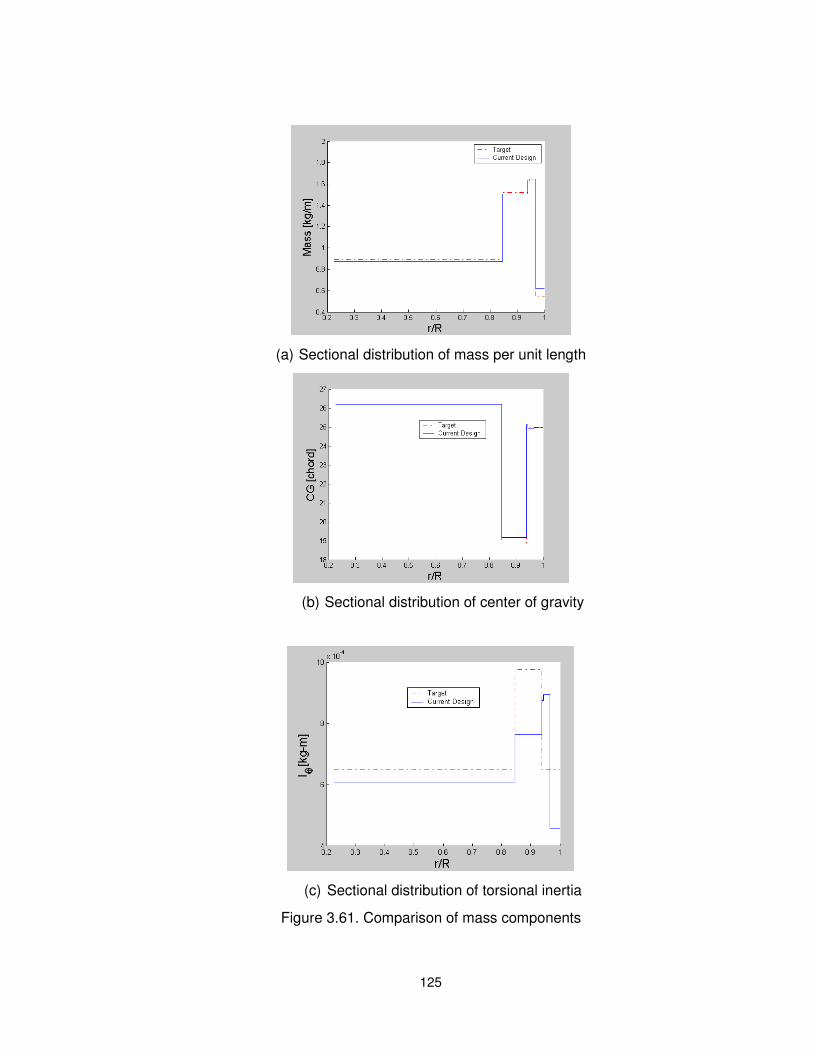
125

(a) Sectional distribution of mass per unit length

(b) Sectional distribution of center of gravity

(c) Sectional distribution of torsional inertia

Figure 3.61. Comparison of mass components

θ

126

3.2.12 Summary of ATR-A design development

As mentioned, the ATR-A example showed the capability to deal with a more complex and

realistic model such as different types of airfoil with different blade planform. The

DYMORE input generating sub-routine is updated to model the blade with linear twist, droop

and swept tip sections making it more stable for this kind of blade. The cases for hinge-less

rotors were successfully executed. Some analyses were done on articulated rotors, but it was

necessary to include a spring at the root for DYMORE in order to compute the frequencies

and modes. At this point, the effect of a spring is not yet well understood and needs further

exploration in future work.

Table 3.56. ATR-A blade final design properties

Section

Final design

Mass Iθ CG loc EA loc Ballast rods

[kg/m] [kg-m] [%c] [%c] Weight

[kg/m]

Location

[%c]

0 0.227~0.847R 0.88 5.78×10-4 25.6 28.5 0.284 6.80

1 0.847~0.938R 1.50 7.69×10-4 19.4 28.5 0.070 3.30

2 0.938~0.943R 1.63 8.84×10-4 25.1 28.5 0.344 6.80

3 0.943~0.965R 1.65 9.57×10-4 25.6 31.7 0.500 12.1

4 0.965~1.000R 0.62 5.20×10-4 26.5 31.7 0.280 6.80

During the pre-processing, the effects of some important parameter have been studied

followed by the optimization process. Once the optimization reached convergence, new loads

corresponding to that optimized design were recalculated using CAMRAD-II. Based on

those loads, another optimization process was run. The results of the application of the new

loads on the design are that the MFC plies move toward the leading edge and the tip twist

angle increased 6.5 % due to a slight decrease on the design loads. Implementation of denser

and stiffer foam on the D-spar region of the cross section helps to reduce the strain generated

on the cross section without significantly affecting the actuation obtained. The foam

127

implementation moved the elastic axis backward and added 0.045kg/m to the weight/length.

Specific diameters of the tungsten rod are used for the ballast weight. Ply drop modeling

reduced the twist rate by 1%. The final design for each section is shown in section 3.2.10 and

the summarized again in Table 3.56.

128

CHAPTER 4

CONCLUSIONS AND RECOMMENDATIONS

This chapter summarizes the main accomplishments of this dissertation. It then makes

conclusions based upon the results from the numerical analysis. Finally, it addresses the

recommendations on some of the important areas for future improvements.

4.1 Summary and main conclusions

In this dissertation, the process to optimally design active twist rotor blades was introduced.

The proposed optimization framework allows for exploring a rich and highly nonlinear

design space in order to maximize twist authority while satisfying a series of constraints.

Different analyses are combined in the framework: cross sectional analysis, an automated

mesh generator, a one-dimensional beam solver, a three-dimensional local strain module, and

numerical optimization routines. The mathematical optimization problem was subdivided in

two loops: the other loop provides critical design loads for the inner loop and only need to

run for a few iterations. With those critical loads, the inner optimization loop was run for

several iterations until an optimum solution was obtained. The design was then passed back

to the outer loop, and the process started again until convergence. This convergence shown to

be fast, which indicates that although the loads changes with changes in blade stiffness and

inertia properties, the critical load values, for structural sizing do not vary much. This allows

the design to be done much faster and effectively. Adjustment to the optimum design was

done at the end to ensure manufacturability of the blade and to take into account limitations

of commercially available materials.

129

Due to the limitations on some of these solvers, resolution strategies were proposed. These

include mesh overlapping, element distortion, trailing edge tab modeling, electrode modeling

and foam implementation of the mesh generator. Also, due to sensitivity of the optimizer to

the initial designs, an approach to generate an initial feasible design was presented.

The effectiveness of the proposed design process has been demonstrated through two

examples. Optimization studies were performed using the existing NASA/Army/MIT ATR

blade case. The first example studied was the ATR-I: by introducing the optimization process,

the original design was able to be further refined and improved. The optimization process

showed that the original design could be improved significantly. The examples showed that

the original ATR blade, successfully manufactured and tested, could exhibit at least a 20%

higher actuation performance level than the original blade if designed within the proposed

optimization framework. The constraint of the elastic axis position with respect to the quarter

chord affects the position of the spar along the cross section. Some passive plies are added

near the nose to reduce the maximum strain and this showed a positive effect on the actuation

authority of the blade.

The second example, ATR-A, presented a much more challenging problem. Based on a

scaled model of AH-60D Apache blade, advanced airfoils, blade planform, MFC integrated

actuator design, and practical blade mechanical target property distribution along its radius

(so to match those of the target rotor system) were introduced to this nonlinear design space.

The proposed nested-loop optimization approach was successfully used. Manufacturing and

other practical constraints were brought to the problem. Several studies were conducted that

investigated the dependence of several blade parameters (e.g., center of gravity, elastic axis,

strain hot spots, torsional frequency, etc.) and blade twist authority to the design variables. It

was shown, for example, that the unmodeled foam can change the elastic axis by as much as

30% chord and the 1st torsional frequency around 20% while basically not affecting the

center of gravity. The effect of placing stiffer foam on the D-spar region of the cross section

is also studied. The distorted element showed a very small effect on the blade properties and

considered to be negligible. The recalculated worst loading case on the inner loop converged

design showed slight decrease and the implementation of those loading to the proposed

130

optimization process showed that the MFC plies moved toward the leading edge about 20%

and increased the active tip twist angle of 6.5%. Based on this optimized design, final designs

along the span which satisfied the target values and also the given constraints are proposed.

These designs are also been carefully adjusted considering the practical manufacture process.

4.2 Key contributions

The following were the key contributions achieved in this dissertation:

• Development of the first mathematical optimization based design framework for

active twist rotor blades

• Introduction of a nested, two-level optimization architecture that speeds up the

optimization process.

• Numerically shown that the already test-flown NASA/Army/MIT ATR blade can

be altered to have a 30% increase in active tip twist while better satisfying its

original target properties

• Complete design of an advanced active twist rotor blade using the new framework.

It is based on 1/6 scale of the AH 64D Apache blade that has 2.5 times more

authority than its predecessor. The design is being built and is scheduled to fly at

NASA’s Transonic Dynamics Tunnel during the fall of 2010.

Several other findings associated with the design sensitivities of active twist blades and the

practical implementations of the concept were introduced in this dissertation.

131

4.3 Recommendation for future work

From the studies conducted in this dissertation, the following areas should be considered for

further studies:

• Change of the optimization method. The gradient-based optimization method used in

this dissertation suffers from the typical shortcomes of this class of optimizer: no

guarantee of global optimum and dependence to the initial guess. Introducing

different optimization methods that are more robust to the initial point or a global

optimization scheme would also be a good option when pursued with careful

consideration to the computational cost.

• Improve on the sensitivity calculation. The sensitivity of the objective function and

constraints were calculated based on direct finite differences. This was done for

simplicity at an increased computational cost. While analytical sensitivity is not

feasible due to the complexity of the problem, there are alternative methods that are

far superior to the simple finite difference (e.g., Adjoint Method).

• Further subdivision of the optimization architecture. While dealing with the ply

thickness as continuous design variables worked well, the manual rounding of their

results to integer multiples of the prepreg nominal thickness slows down the

optimization process. This could be avoided by using the stiffness and mass constants

as design variables and setup a separate inverse optimization in which ply thickness

and angles need to be determined to match the target stiffness and mass constants

coming from the other optimization loop.

• Further study on the relative frequency of loads calculation. Although the inner-outer

loop separation proved to work very well for the cases studied in this dissertation,

more studies are recommended. By extending the implemented formulation such that

132

both the inner and outer loops are part of the same Matlab code, one could better

quantify the frequency needed for the critical loads to be recalculated. Moreover, this

is expected to be a function of the initial design and flight conditions.

• Introduction of a dynamic objective function. Instead of maximizing static tip twist, a

more interesting objective function would be to maximize the tip twist at (N-1)P, NP,

and (N+1)P, where N represents the number of blades and P the blade passage

frequency. This reflects the ultimate goal that is to maximize blade control authority

for vibration reduction at the frequency range of interest.

133

Appendix 1. ATR optimization code structure

The structure of the code used in this dissertation is presented below. Blocks indicate the sub

folders and the files under that folder. The first column shows the sequence of the file called,

with the heritage being associated with the origin of the call. The file name itself is quite self

–explanatory but the last column gives some additional information.

134

Appendix 2. Maximum loads for ATR-I by CAMRAD II

Max loads for Torsion case (in - lb)

0.2R 0.3R 0.4R 0.5R 0.6R 0.7R 0.8R 0.9R

-11.7 -10.7 -9.6 -7.8 -6.6 -5.1 -3.3 -1.8

6.2 4.2 3.2 3.9 5.2 3.5 2.7 1

-10.7 -11.15 -10.2 -5.9 -8.05 -4 -2.9 -1.55

Max loads for Flap-wise bending case (in -lb)

0.2R 0.3R 0.4R 0.5R 0.6R 0.7R 0.8R 0.9R

-11.7 -10.7 -9.6 -7.8 -6.6 -5.1 -3.3 -1.8

6.2 4.2 3.2 3.9 5.2 3.5 2.7 1

-10.7 -11.15 -10.2 -5.9 -8.05 -4 -2.9 -1.55

Max loads for Lag-wise bending case (in - lb)

0.2R 0.3R 0.4R 0.5R 0.6R 0.7R 0.8R 0.9R

-11.7 -10.7 -9.6 -7.8 -6.6 -5.1 -3.3 -1.8

6.2 4.2 3.2 3.9 5.2 3.5 2.7 1

-10.7 -11.15 -10.2 -5.9 -8.05 -4 -2.9 -1.55

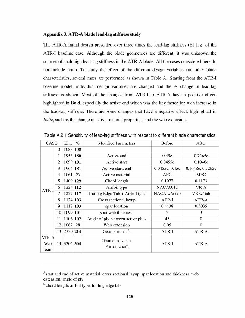
135

Appendix 3. ATR-A blade lead-lag stiffness study

The ATR-A initial design presented over three times the lead-lag stiffness (EI_lag) of the

ATR-I baseline case. Although the blade geometrics are different, it was unknown the

sources of such high lead-lag stiffness in the ATR-A blade. All the cases considered here do

not include foam. To study the effect of the different design variables and other blade

characteristics, several cases are performed as shown in Table A.. Starting from the ATR-I

baseline model, individual design variables are changed and the % change in lead-lag

stiffness is shown. Most of the changes from ATR-I to ATR-A have a positive effect,

highlighted in Bold, especially the active end which was the key factor for such increase in

the lead-lag stiffness. There are some changes that have a negative effect, highlighted in

Italic, such as the change in active material properties, and the web extension.

Table A.2.1 Sensitivity of lead-lag stiffness with respect to different blade characteristics

5 start and end of active material, cross sectional layup, spar location and thickness, web extension, angle of ply 6 chord length, airfoil type, trailing edge tab

CASE EIlag % Modified Parameters Before After

ATR-I

0 1088 100

1 1953 180 Active end 0.45c 0.7265c

2 1099 101 Active start 0.0455c 0.1048c

3 1964 181 Active start, end 0.0455c, 0.45c 0.1048c, 0.7265c

4 1061 98 Active material AFC MFC

5 1409 129 Chord length 0.1077 0.1173

6 1224 112 Airfoil type NACA0012 VR18

7 1277 117 Trailing Edge Tab + Airfoil type NACA w/o tab VR w/ tab

8 1124 103 Cross sectional layup ATR-I ATR-A

9 1118 103 spar location 0.4438 0.5035

10 1099 101 spar web thickness 2 3

11 1106 102 Angle of ply between active plies 45 0

12 1067 98 Web extension 0.05 0

13 2330 214 Geometric var5. ATR-I ATR-A

ATR-A

W/o

foam

14 3305 304 Geometric var. +

Airfoil char6. ATR-I ATR-A

136

Appendix 4. Maximum loads for Case T1(b) by CAMRAD II

138

Appendix 5. Refined ATR-A main blade mass stiffness and actuation matrices (SI unit)

With the baseline material properties (w/ foam):

. . . . . x . x

. . . . x . .

. . . . x . .m

. . x . x . x . .

. x . . . . x . x

. x . . . .

− −

−

−

− −

− − −

−

−

− −

=

−

−

4 3

4

3

4 3

4 5 7

3

4

0 89 0 00 0 00 0 00 2 81 10 1 23 10

0 00 0 89 0 00 2 81 10 0 00 0 00

0 00 0 00 0 89 1 23 10 0 00 0 00

0 00 2 81 10 1 23 10 6 02 10 0 00 0 00

2 81 10 0 00 0 00 0 00 1 30 10 3 97 10

1 23 10 0 00 0 00 0 00 3 9 x . x− −

7 47 10 5 89 10

. x . . . . x . x

. . x . x . x . x . x

. . x . x . x . . xk

. . x . x . . . x

. x . x .

− −

−

−

−

− − − − −

− −

− −=

− − − −

−

6 3 4

3

5 4 2 1 1

4 4 2 2

2 2 3

1

332 10 32 92 4 61 0 084 1 38 10 384 10

32 92 6 27 10 1 32 10 213 10 179 10 1 62 10

4 61 132 10 4 02 10 1 64 10 0 70 756 10

0 084 213 10 1 64 10 65 73 0 39 417 10

1 38 10 1 79 10 0 . . .

. x . x . x . x . . x− − −

− −

− − − −

4 1 2 3 3

70 0 39 63 97 811

384 10 1 62 10 7 56 10 417 10 811 334 10

[ ]T( a )F 0.8578 4.5885 14.7767 -3.0453 0.0409 0.0002=

With the commercially available material properties (w/ foam):

. . . . . x . x

. . . . x . .

. . . . x . .m

. . x . x . x . .

. x . . . . x . x

. x . . . .

− −

−

−

− −

− − −

−

−

− −

=

−

−

4 3

4

3

4 3

4 5 7

3

4

0 89 0 00 0 00 0 00 2 81 10 1 26 10

0 00 0 89 0 00 2 81 10 0 00 0 00

0 00 0 00 0 89 1 26 10 0 00 0 00

0 00 2 81 10 1 26 10 6 02 10 0 00 0 00

2 81 10 0 00 0 00 0 00 1 30 10 3 97 10

1 26 10 0 00 0 00 0 00 3 9 x . x− −

7 47 10 5 89 10

. x . . . . x . x

. . x . x . x . x . x

. . x . x . x . . xk

. . x . x . . . x

. x . x .

− −

−

−

−

− − − − −

− −

− −=

− − − −

−

6 3 4

3

5 4 2 1 1

4 4 2 2

2 2 3

1

3 48 10 34 66 4 85 0 086 1 47 10 3 95 10

34 66 6 32 10 1 39 10 210 10 1 95 10 1 69 10

4 85 1 39 10 4 20 10 1 76 10 0 75 814 10

0 084 210 10 1 76 10 65 95 0 39 4 23 10

1 47 10 1 95 10 0 . . .

. x . x . x . x . . x− − −

− −

− − − −

4 1 2 3 3

75 0 39 66 70 8 92

3 95 10 1 69 10 814 10 4 23 10 8 92 3 51 10

[ ]T( a )F 0.8666 4.8535 15.5423 -3.0467 0.0413 0.0002=

where the standard convention of extension, transverse shear (chordwise), transverse shear

(flapwise), torsion, flapwise bending, and lead-lag bending is used in this sequence.

139

Appendix 6. Refined ATR-A Root design mass and stiffness matrices (SI unit)

With the baseline material properties (w/o foam):

STIFFNESS_MATRIX : Option 1

2.49 x107 2.27 x102 6.08 x103 -1.29 x103 -6.55 x103 -4.91 x104

2.27 x102 7.86 x106 1.06 x103 -1.74 x103 5.82 x102 11.5

6.08 x103 1.06 x103 1.13 x105 -1.32 x103 -5.29 -32.7

-1.29 x103 -1.74 x103 -1.32 x103 2.15 x102 2.27E-01 -3.42

-6.55 x103 5.82 x102 -5.29 2.27E-01 3.05 x102 15.3

-4.91 x104 11.5 -32.7 -3.42 15.3 6.76 x103

MASS_MATRIX (w/o ballast weight): Option 1

7.77 x10-1 0.0 0.0 0.0 -2.08 x10-4 -1.43 x10-3

0.0 7.77 x10-1 0.0 -2.08 x10-4 0.0 0.0

0.0 0.0 7.77 x10-1 -1.43 x10-3 0.0 0.0

0.0 -2.08 x10-4 -1.43 x10-3 2.25 x10-4 0.0 0.0

-2.08 x10-4 0.0 0.0 0.0 1.03 x10-5 3.69 x10-7

-1.43 x10-3 0.0 0.0 0.0 3.69 x10-7 2.14 x10-4

With the commercially available material properties (w/o foam):

STIFFNESS_MATRIX : Option 1

2.82 x107 1.30 x102 7.42 x103 -1.48 x103 -7.42 x103 -5.43 x104

1.30 x102 8.83 x106 6.61 x103 -2.07 x103 6.64 x102 11.1

7.42 x103 6.61 x103 1.19 x105 -1.59 x103 -5.7629 -35.9

-1.48 x103 -2.07 x103 -1.59 x103 2.32 x102 2.43E-01 -4.52

-7.42 x103 6.64 x102 -5.7629 2.43E-01 3.45 x102 15.3

-5.43 x104 11.1 -35.9 -4.52 15.3 7.67 x103

MASS_MATRIX (Before implementing ballast weight): Option 1

7.79 x10-1 0.0 0.0 0.0 -2.09 x10-4 -1.3943 x10-3

0.0 7.79 x10-1 0.0 2.09 x10-4 0.0 0.0

0.0 0.0 7.79 x10-1 1.39 x10-3 0.0 0.0

0.0 2.09 x10-4 1.39 x10-3 2.25 x10-4 0.0 0.0

-2.09 x10-4 0.0 0.0 0.0 1.03 x10-5 3.59 x10-7

-1.39 x10-3 0.0 0.0 0.0 3.59 x10-7 2.15 x10-4

140

Appendix 7. Refined ATR-A Tip layup mass and stiffness matrices (SI unit)

With the baseline material properties (w/o foam):

STIFFNESS_MATRIX

1.40 x106 0.0 0.0 0.0 -5.36 x102 -3.03 x104

0.0 2.38E+05 8.41 x102 -74.6 0.0 0.0

0.0 8.41 x102 1.39 x104 1.32 x102 0.0 0.0

0.0 -74.6 1.32 x102 20.7 0.0 0.0

-5.36 x102 0.0 0.0 0.0 30.5 11.6

-3.03 x104 0.0 0.0 0.0 11.6 2.01 x103

MASS_MATRIX (Before implementing ballast weight)

1.24 x10-1 0.0 0.0 0.0 -4.76 x10-5 -2.69 x10-3

0.0 1.24 x10-1 0.0 4.76 x10-5 0.0 0.0

0.0 0.0 1.24 x10-1 2.69 x10-3 0.0 0.0

0.0 4.76 x10-5 2.69 x10-3 1.81 x10-4 0.0 0.0

-4.76 x10-5 0.0 0.0 0.0 2.71 x10-6 1.03 x10-6

-2.69 x10-3 0.0 0.0 0.0 1.03 x10-6 1.78 x10-4

MASS_MATRIX (After implementing ballast weight)

4.11 x10-1 0.0 0.0 0.0 -9.43 x10-5 3.42 x10-3

0.0 4.11 x10-1 0.0 9.43 x10-5 0.0 0.0

0.0 0.0 4.11 x10-1 -3.42 x10-3 0.0 0.0

0.0 9.43 x10-5 -3.42 x10-3 3.12 x10-4 0.0 0.0

-9.43 x10-5 0.0 0.0 0.0 2.71 x10-6 -7.85 x10-7

3.42 x10-3 0.0 0.0 0.0 -7.85 x10-7 3.09 x10-4

With the commercially available material properties (w/o foam):

STIFFNESS_MATRIX

1.40 x106 0.0 0.0 0.0 -5.36 x102 -3.03 x104

0.0 2.38E+05 8.41 x102 -74.6 0.0 0.0

0.0 8.41 x102 1.39 x104 1.32 x102 0.0 0.0

0.0 -74.6 1.32 x102 20.7 0.0 0.0

-5.36 x102 0.0 0.0 0.0 30.5 11.6

-3.03 x104 0.0 0.0 0.0 11.6 2.01 x103

141

MASS_MATRIX (Before implementing ballast weight)

1.24 x10-1 0.0 0.0 0.0 -4.76 x10-5 -2.69 x10-3

0.0 1.24 x10-1 0.0 4.76 x10-5 0.0 0.0

0.0 0.0 1.24 x10-1 2.69 x10-3 0.0 0.0

0.0 4.76 x10-5 2.69 x10-3 1.81 x10-4 0.0 0.0

-4.76 x10-5 0.0 0.0 0.0 2.71 x10-6 1.03 x10-6

-2.69 x10-3 0.0 0.0 0.0 1.03 x10-6 1.78 x10-4

MASS_MATRIX (After implementing ballast weight)

4.11 x10-1 0.0 0.0 0.0 -9.43 x10-5 3.42 x10-3

0.0 4.11 x10-1 0.0 9.43 x10-5 0.0 0.0

0.0 0.0 4.11 x10-1 -3.42 x10-3 0.0 0.0

0.0 9.43 x10-5 -3.42 x10-3 3.12 x10-4 0.0 0.0

-9.43 x10-5 0.0 0.0 0.0 2.71 x10-6 -7.85 x10-7

3.42 x10-3 0.0 0.0 0.0 -7.85 x10-7 3.09 x10-4

142

BIBLIOGRAPHY

Aoyama, T., C. Yang, N. Kondo and S. Saito (2006). Comparison of Noise Reduction Effect between Afc and Conventional Ibc by Moving Overlapped Grid Method. 12th AIAA/CEAS Aeroacoustics Conference (27th AIAA Aeroacoustics Conference), Cambridge, MA.

Barrett, R. M. (1990). Intelligent Rotor Blade and Structures Development Using Directionally Attached Piezoelectric Crystals College park, The University of Maryland Master of Science.

Bauchau, O. A. (1998). "Computational Schemes for Flexible Nonlinear Multi-Body Systems." Multibody System Dynamics 2: pp. 169–225.

Bauchau, O. A. (2008). "Review of Contemporary Approaches for Constraint Enforcement in Multibody Systems." Journal of Computational and Nonlinear Dynamics 3(1): 011005-1-8.

Bent, A. A. and N. W. Hagood (1997). "Piezoelectric Fiber Composites with Interdigitated Electrodes." Journal of Intelligent Material Systems and Structures 8(11): 903-919.

Bent, A. A., N. W. Hagood and J. P. Rodgers (1995). "Anisotropic Actuation with Piezoelectric Fiber Composites." Journal of Intelligent Material Systems and Structures 6(3): 338-349.

Bernhard, A. P. F. and J. Wong (2003). Sikorsky Active Rotor Control Evaluation of Nasa/Army/Mit Active Twist Rotor. American Helicopter Society Society 59th Annual Forum, Phoenix, AR.

Booth, E. R. and M. L. Wilbur (2004). "Acoustic Aspects of Active-Twist Rotor Control." Journal of the American Helicopter Society 49(1): 3-10.

Brockmann, T. H. and R. Lammering (2006). "Beam Finite Elements for Rotating Piezoelectric Fiber Composite Structures." Journal Of Intelligent Material Systems and Structures(5): 431.

Brown, E. L. (2003). Integrated Strain Actuation in Aircraft with Highly Flexible Composite Wings. Cambridge, MA, Massachusetts Institute of Technology. Doctor of

Philosophy.

Celi, R. (1999). "Recent Applications of Design Optimization to Rotorcraft - a Survey." Journal of Aircraft 36(1): 176-189.

Centolanza, L. R. (2002). "Induced-Shear Piezoelectric Actuators for Active Twist Rotor Blades." Collection of Technical Papers - AIAA/ASME/ASCE/AHS/ASC Structures, Structural Dynamics and Materials Conference 3: 1977-1987.

Cesnik, C. E. S., J. Mok, J. A. Morillo and A. S. Parikh (2005). Design Optimization of Active Twist Rotor Blades. 30th European Rotorcraft Forum, Marseilles, France.

Cesnik, C. E. S., J. Mok, A. S. Parikh and S. Shin (2004). Optimum Design Framework for Integrally Twisted Helicopter Blades 45th AIAA/ASME/ASCE/AHS/ASC

143

Structures, Structural Dynamics and Materials Conference, Palm Springs, California.

Cesnik, C. E. S. and R. Palacios (2003). Modeling Piezocomposite Actuators Embedded in Slender Structures. AIAA/ASME/ASCE/AHS/ASC 44th Structures, Structural Dynamics and Materials Conference- Adaptive Structures, Norfolk, VA.

Cesnik, C. E. S., R. S. Park and R. Palacios (2003). "Effective Cross-Section Distribution of Anisotropic Piezocomposite Actuators for Wing Twist." Smart Structures and Materials 2003: Smart Structures and Integrated Systems 5056: 21-32.

Cesnik, C. E. S., S.-J. Shin, W. K. Wilkie, M. L. Wilbur and P. H. Mirick (1999). Modeling, Design, and Testing of the Nasa/Army/Mit Active Twist Rotor Prototype Blade. American Helicopter Society 55th Annual Forum, Montreal, Canada

Cesnik, C. E. S. and S. Shin (2001). "On the Modeling of Integrally Actuated Helicopter Blades." International Journal of Solids and Structures 38(10-13): 1765-1789.

Cesnik, C. E. S. and S. J. Shin (2001). "On the Twist Performance of a Multiple-Cell Active Helicopter Blade." Smart Materials & Structures 10(1): 53-61.

Cesnik, C. E. S., S. J. Shin and M. L. Wilbur (2001). "Dynamic Response of Active Twist Rotor Blades." Smart Materials & Structures 10(1): 62-76.

Chen, P. C. and I. Chopra (1996). "Induced Strain Actuation of Composite Beams and Rotor Blades with Embedded Piezoceramic Elements." Smart Materials and Structures(1): 35.

Chopra, I. (2000). "Status of Application of Smart Structures Technology to Rotorcraft Systems." Journal of the American Helicopter Society 45(4): 228-252.

Chopra, I. (2002). "Review of State of Art of Smart Structures and Integrated Systems." Aiaa Journal 40(11): 2145-2187.

Cribbs, R. C. and P. P. Friedmann (2001). Actuator Saturation and Its Influence on Vibration Reduction by Actively Controlled Flaps. 42nd AIAA/ASME/ASCE/AHS/ASC Structures, Structural Dynamics, and Materials Conference, Reston, VA.

Davis, M. W. and W. H. Wellert (1991). "Helicopter Rotor Dynamics Optimization with Experimental Verification." Journal of Aircraft 28(1): 38-48.

Depailler, G. and P. P. Friedmann (2002). Reduction of Vibrations Due to Dynamic Stall in Helicopters Using an Actively Controlled Flap. 43rd AIAA/ASME/ASCE/AHS/ASC Structures, Structural Dynamics, and Materials Conference, Denver, Colorado.

Fletcher, R. and M. J. D. Powell (1963). "A Rapidly Convergent Descent Method for Minimization." Journal of Computational and Nonlinear Dynamics 6: pp. 163-168.

Friedmann, P. P. (1977). "Recent Developments in Rotary-Wing Aeroelasticity." Journal of Aircraft 14(11): 1027-1041.

Friedmann, P. P. (1987). "Recent Trends in Rotary-Wing Aeroelasticity." Vertica 11(1-2): 139-170.

Friedmann, P. P. (1990). "Helicopter Rotor Dynamics and Aeroelasticity - Some Key Ideas and Insights." Vertica 14(1): 101-121.

Friedmann, P. P. (1991). "Helicopter Vibration Reduction Using Structural Optimization with Aeroelastic Multidisciplinary Constraints - a Survey." Journal of Aircraft 28(1): 8-21.

Friedmann, P. P. (1999). "Renaissance of Aeroelasticity and Its Future." Journal of Aircraft

144

36(1): 105-121.

Friedmann, P. P. (2004). "Rotary-Wing Aeroelasticity: Current Status and Future Trends." AIAA Journal 42(10): 1953-1972.

Friedmann, P. P., G. P. Carman and T. A. Millott (2001). "Magnetostrictively Actuated Control Flaps for Vibration Reduction in Helicopter Rotors - Design Considerations for Implementation." Mathematical and Computer Modelling 33(10-11): 1203-1217.

Friedmann, P. P. and D. H. Hodges (2003). "Rotary Wing Aeroelasticity - a Historical Perspective." Journal of Aircraft 40(6): 1019-1046.

Friedmann, P. P. and T. A. Millott (1995). "Vibration Reduction in Rotorcraft Using Active Control - a Comparison of Various Approaches." Journal of Guidance Control and Dynamics 18(4): 664-673.

Friedmann, P. P. and P. Shanthakumaran (1984). "Optimum Design of Rotor Blades for Vibration Reduction in Forward Flight." Journal of the American Helicopter Society 29(4): 70-90.

Friedmann, P. P., C. Venkatesan and K. Yuan (1992). Development of a Structural Optimization Capability for the Aeroelastic Tailoring of Composite Rotor Blades with Straight and Swept Tips. 4th AIAA/USAF/NASA/OAI Symposium on Multidisciplinary Analysis and Optimization, Cleveland, OH.

Fulton, M. and R. A. Ormiston (1998). Small-Scale Rotor Experiments with on-Blade Elevons to Reduce Blade Vibratory Loads in Forward Flight. Proceedings of the 54th Annual Forum of the American Helicopter Society, Alexandria, VA.

Ganguli, R. (2004). "Survey of Recent Developments in Rotorcraft Design Optimization." Journal of Aircraft 41(3): 493-510.

Glaz, B. (2008). Active/Passive Optimization of Helicopter Rotor Blades for Improved Vibration, Noise, and Performance Characteristics. Aerospace Engineering, University of Michigan. Doctor of Philosophy.

Glaz, B., P. P. Friedmann and L. Lui (2006). Surrogate Based Optimization of Helicopter Rotor Blades for Vibration Reduction in Forward Flight. 47th AIAA/ASME/ASCE/AHS/ASC Structures, Structural Dynamics, and Materials Conference, Newport, Rhode Island.

Glukhikh, S., E. Barkanov, A. Kovalev, P. Masarati, M. Morandini, J. Riemenschneider and P. Wierach (2008). "Design of Helicopter Rotor Blades with Actuators Made of a Piezomacrofiber Composite." Mechanics of Composite Materials 44(1): 57-64.

Grohmann, B. A., C. Maucher, T. Prunhuber, P. Jänker, O. Dieterich, B. Enenkl, M. Bauer, E. Ahci, A. Altmikus and H. Baier (2008). "Multidisciplinary Design and Optimization of Active Trailing Edge for Smart Helicopter Rotor Blade." Mechanics of Advanced Materials and Structures 15(3): 307-324.

Hafka, R. T. and Z. Gurdal (1992). Elements of Structural Optimization, Kluwer Academic Publishers.

Hoffmann, F., S. Opitz and J. Riemenschneider (2009). Validation of Active Twist Modeling Based on Whirl Tower Tests. American Helicopter Society 65th Annual Forum, Grapevine, Texas, USA.

Hooper, W. E. (1984). " Vibratatory Airloading of Helicopter Rotors." Vertica 8(2): 73–92.

145

Johnson, W. (1992-1997). Camrad. CAMRAD II, Comprehensive Analytical Model of Rotorcraft Aerodynamics and Dynamics. W. Johnson. Palo Alto, California, Johnson Aeronautics.

Jones, R. M. (1999). Mechanics of Composite Materials, Taylor & Francis

Kovalovs, A., E. Barkanov and S. Gluhihs (2007). "Active Twist of Model Rotor Blades with D-Spar Design " Transport. Vilnius: Technika 22(1): 38-44.

Lemos, R. (2007). The Helicopter: A Hundred Years of Hovering.

Lim, J. w. and I. Chopra (1991). "Aeroelastic Optimization of a Helicopter Rotor." Journal of Aircraft 28(1): 29-37.

Milgram, J. and I. Chopra (1998). "A Parametric Design Study for Actively Controlledtrailing Edge Flaps." Journal of the American Helicopter Society 43(2): 110-119.

Millott, T. A. and P. P. Friedmann. (1994). Vibration Reduction in Helicopter Rotors

Using an Actively Controlled Partial Span Trailing Edge Flap Located on the Blade. NASA-CR-4611.

Monner, H. P., S. Opitz, J. Riemenschneider and P. Wierach (2008). Evolution of Active Twist Rotor Designs at Dlr. 49th AIAA/ASME/ASCE/AHS/ASC Structures, Structural Dynamics, and Materials Conference, Schaumburg, IL.

MSCSoftware (2004). Patran. Santa Ana, CA.

Palacios Nieto, R. (2005). Asymptotic Models of Integrally-Strained Slender Structures for High-Fidelity Nonlinear Aeroelastic Analysis. Aerospace Engineering. Ann Arbor, University of Michigan. Doctor of Philosophy.

Pape, A. L. and P. Beaumier (2005). "Numerical Optimization of Helicopter Rotor Aerodynamic Performance in Hover." Aerospace Science and Technology 9: 191-201.

Philippe, J.-J. (2003). "Rotorcraft Challenges and Associated French-German Research Contributions." AIAA/ICAS International Air and Space Symposium and Exposition: The Next 100 Years; Dayton, OH; July 14-17, 2003.

Prahlad, H. and I. Chopra (2007). "Modeling and Experimental Characterization of Sma Torsional Actuators." Journal of Intelligent Material Systems and Structures 18(1): 29-38.

Prechtl, E. F. (2000). Design and Implementation of a Piezoelectric Servoflap Actuation System for Helicopter Roror Individual Blade Control. Aeronautics and Astronautics, Massachusetts Institute of Technology. Doctor of Philosophy.

Rodgers, J. P. (1999). Development of an Integral Twist-Actuated Rotor Blade for Individual Blade Control. Aeronautics and Astronautics, Massachusetts Institute of Technology. Doctor of Philosophy.

Rodgers, J. P. and N. W. Hagood (1998). Preliminary Mach-Scale Hover Testing of an Integral Twist-Actuated Rotor Blade, SPIE.

Sanders, B. (2004). "Defense Advanced Research Projects Agency - Smart Materials and Structures Demonstration Program Overview." Journal of Intelligent Material Systems and Structures 15(4): 227-233.

Sekula, M. K. (2005). "A Parametric Study of the Structural Design for an Advanced Active

146

Twist Rotor." Annual forum proceedings. 1: 95.

Shaw, J., N. Albion, E. J. Hanker Jr. and R. S. Teal (1989). "Higher Harmonic Control: Wind Tunnel Demonstration of Fully Effective Vibratory Hub Force Suppression " Journal of the American Helicopter Society Jan 1989 1 14-25 34 1.

Shin, S., C. Cesnik and M. L. Wilbur (2000). Dynamic Response of Active Twist Rotor Blade. AIAA/ASME/AHS Adaptive Structures Forum, Atlanta, Georgia.

Shin, S. and C. E. S. Cesnik (1999). Design, Manufacturing and Testing of an Active Twist Rotor, Active Materials and Structures Laboratory, AMSL Report #99-3, Massachusetts Institute of Technology.

Shin, S. and C. E. S. Cesnik (2007). "Helicopter Vibration Reduction in Forward Flight Using Blade Integral Twist Actuation." Journal of Mechanical Science and Technology 21(2): 251-263.

Shin, S., C. E. S. Cesnik and S. R. Hall (2005). "Closed-Loop Control Test of the Nasa/Army/Mit Active Twist Rotor for Vibration Reduction." Journal of the American Helicopter Society 50(2): 178-194.

Shin, S., C. E. S. Cesnik and S. R. Hall (2007). "Design and Simulation of Integral Twist Control for Helicopter Vibration Reduction." International Journal of Control Automation and Systems 5(1): 24-34.

Shin, S. J. (1999). Design Manufacturing and Testing of an Active Twist Rotor. Aeronautics and Astronautics, Massachusetts Institute of Technology. Master of Science.

Shin, S. J., C. E. S. Cesnik and S. R. Hall (2005). "System Identification Technique for Active Helicopter Rotors." Journal of Intelligent Material Systems and Structures 16(11-12): 1025-1038.

Shin, S. J., C. E. S. Cesnik, W. K. Wilkie and M. L. Wilbur (2008). "Design and Manufacturing of a Model-Scale Active Twist Rotor Prototype Blade." Journal of Intelligent Material Systems and Structures 19(12): 1443-1456.

Viswamurthy, S. R. and R. Ganguli (2004). "An Optimization Approach to Vibration Reduction in Helicopter Rotors with Multiple Active Trailing Edge Flaps." Aerospace Science and Technology 8: 185-194.

Wickramasinghe, V. K. and N. W. Hagood (2004). "Durability Characterization of Active Fiber Composite Actuators for Helicopter Rotor Blade Applications." Journal of Aircraft 41(4): 931-937.

Wierach, P., J. Riemenschneider and S. Keye (2005). Development of an Active Twist Rotor Blade with Distributed Actuation and Orthotropic Material, SPIE.

Wilbur, M. L., P. H. Mirick, W. T. Yeager, C. W. Langston, C. E. S. Cesnik and S. Shin (2002). "Vibratory Loads Reduction Testing of the Nasa/Army/Mit Active Twist Rotor." Journal of the American Helicopter Society 47(2): 123-133.

Wilbur, M. L., P. H. Mirick, W. T. J. Yeager, C. W. Langston, C. E. S. Cesnik and S. J. Shin (2001). Vibratory Loads Reduction Testing of the Nasa/Army/Mit Active Twist Rotor. American Helicopter Society 57th Annual Forum, Washington, D. C.

Wilbur, M. L., W. T. Yeager, Jr. and M. K. Sekula (2001). Further Examination of the Vibratory Loads Reduction Results from the Nasa/Army/Mit Active Twist Rotor. American Helicopter Society 58th Annual Forum, Montréal, Canada.

147

Wilkie, W. K. (1997). Anisotropic Piezoelectric Twist Actuation of Helicopter Rotor Blades: Aeroelastic Analysis and Design Optimization. Department of Aerospace Engineering Sciences, University of Colorado. Doctor of Philosophy.

Wilkie, W. K., R. G. Bryant, J. W. High, R. L. Fox, R. F. Hellbaum, J. Antony Jalink, B. D. Little and P. H. Mirick (2000). Low-Cost Piezocomposite Actuator for Structural Control Applications. SPIE’s 7th Annual International Symposium on Smart Structures and Materials, Newport Beach, CA,.

Wilkie, W. K., M. L. Wilbur, P. H. Mirick, C. E. S. Cesnik and S. J. Shin (1999). Aeroelastic Analysis of the Nasa/Army/Mit Active Twist Rotor. American Helicopter Society 55th Annual Forum, Montreal, Canada.

Williams, R. B., D. J. Inman and W. K. Wilkie (2004). "Temperature-Dependent Thermoelastic Properties for Macro Fiber Composite Actuators." Journal of Thermal Stresses 27(10): 903-915.

Williams, R. B., D. J. Inman and W. K. Wilkie (2006). "Nonlinear Response of the Macro Fiber Composite Actuator to Monotonically Increasing Excitation Voltage." Journal of Intelligent Material Systems and Structures 17(7): 601-608.

Young, D. K. and F. J. Tarzanin (1993). "Structural Optimization and Mach Scale Test Validation of a Low Vibration Rotor." Journal of the American Helicopter Society 38(3): 83-92.

Design Optimization for Active Twist Rotor Blades

Documents

Transcript of Design Optimization for Active Twist Rotor Blades