
Design of Progressive Additional Lens with Wavefront ...
96
Design of Progressive Additional Lens with Wavefront Tracing Method A DISSERTATION SUBMITTED TO THE FACULTY OF THE GRADUATE SCHOOL OF THE UNIVERSITY OF MINNESOTA BY Fanhuan Zhou IN PARTIAL FULFILLMENT OF THE REQUIREMENTS FOR THE DEGREE OF Doctor Of Philosophy September, 2010
Transcript of Design of Progressive Additional Lens with Wavefront ...
Design of Progressive Additional Lens with
Wavefront Tracing Method
A DISSERTATION
SUBMITTED TO THE FACULTY OF THE GRADUATE SCHOOL
OF THE UNIVERSITY OF MINNESOTA
BY
Fanhuan Zhou
IN PARTIAL FULFILLMENT OF THE REQUIREMENTS
FOR THE DEGREE OF
Doctor Of Philosophy
September, 2010

c⃝ Fanhuan Zhou 2010
ALL RIGHTS RESERVED

Acknowledgements
I would like to thank my advisor Prof. Fadil Santosa for all his advice and dis-
cussions. I always feel fortunate that Prof. Santosa introduced me to the area of
Progressive Lens Design. His positive attitude toward research, his patience on
my research and his broad vision in applied math always inspired me. I am also
grateful for his careful reading of this thesis. Without his help, it would not be
possible for finish this thesis.
I would like to thank Prof. Robert Gulliver for reviewing my work and serving
as the chair of the committee of my thesis defense. The discussions with Prof.
Gulliver on Differential Geometry extended my understanding of lens design. I
would also like to thank Prof. Bernardo Cockburn and Prof. Hui Zou serving as
committee members on my thesis.
I would like to thank Prof. Fadil Santosa, John Dodson, and MCIM for the
internship opportunity in Ameriprise Financial, which raised my research interest
in Financial Mathematics.
Certainly, I am grateful to my family, especially my parents for consistent
support during my study in USTC and UMN. Their encouragement always keeps
me going forward. I dedicate this thesis to them. Finally, I would want to take
a chance to thank my teachers and friends in the last twenty-two years of study.
My life would be a lot different without their help.
i

Abstract
Progressive addition lenses (PAL) are corrective lenses prescribed to patients
with presbyopia. In PAL power varies smoothly over the lens, allowing the wearer
to compensate for both far vision and near vision corrections. A PAL lens comprise
of at least one complex surface to meet the requirement of having variable power
depending on the gaze direction. A typical PAL consists of a large distance zone
with low power on the upper portion of the lens, a small near distance zone with
higher power on the lower part, and a corridor of increasing power connecting
these two zones smoothly and progressively.
In this work, we investigate a variational approach to PAL design problem in
which a cost function consists of two parts. The first part, when small, implies
that the power distribution is close to the desired one. The second part, when
minimized, makes the optical aberrations small. The goal is to minimize the cost
function.
Previous work on progressive additional lens uses approximations of the phys-
ical optics involved in propagation and refraction of light. These approximations
simplify the calculation of power and astigmatism, a first order aberration, to
knowledge of the principal curvatures of the lens surfaces, and are not capable
of calculating higher order aberrations. To better evaluate the properties of the
optical system, we use geometrical optics. This involves tracing an optical ray
through the lens and calculating how the incident wavefront is altered through
propagation and refraction. The approach is to form a third-order Taylor ex-
pansion of the wavefront at the ray. We develop formulas that relate the Taylor
coefficients as the wavefront propagates and as it is refracted. These higher order
Taylor coefficients are important in understanding optical aberrations.
The formulas we derived can be used to accurately calculate optical properties
of a progressive additional lens. For numerical implementation, we use a tensor-
product B-spline to represent the lens surfaces. Properties of a lens in a given gaze
ii
direction can be calculated by performing numerical calculations. In this way, the
PAL design problem can formulated as a numerical optimization problem in which
lens properties over a set of gaze directions are optimized. The formulation can
be applied to front surface or back surface lens design.
The optimization problem can be solved numerically by a number of methods.
We consider gradient descent method, Newton’s method and the quasi-Newton
method. As a demonstration of the approach proposed in this work, we provide
an example of a progressive addition lens whose front surface is optimized.
iii

Contents
Acknowledgements i
Abstract ii
1 Introduction 1
2 Theory of surfaces 7
2.1 The First Fundamental Form and the Second Fundamental Form 7
2.2 Christoffel symbols and the equations of Weingarten . . . . . . . . 8
2.3 The Third Order Surface coefficients . . . . . . . . . . . . . . . . 9
2.3.1 Approximation of a surface . . . . . . . . . . . . . . . . . . 12
2.4 Principal curvatures and principle directions . . . . . . . . . . . . 13
2.5 Rotation of Principal Coordinates . . . . . . . . . . . . . . . . . . 15
3 Geometric Optics and Lens Design 16
3.1 Geometric optics principles . . . . . . . . . . . . . . . . . . . . . . 16
3.2 Characterizing lens performance with a wavefront . . . . . . . . . 18
3.3 Wavefront aberration and Zernike polynomials . . . . . . . . . . . 19
3.4 Lens design problem . . . . . . . . . . . . . . . . . . . . . . . . . 22
4 Wavefront deformation through smooth refracting lens surface 24
4.1 Wavefront tracing through optical system . . . . . . . . . . . . . . 24
4.2 J. Kneisly’s Approach . . . . . . . . . . . . . . . . . . . . . . . . 25
iv
4.3 Wavefront surface coefficients on propagation . . . . . . . . . . . . 29
4.3.1 The Second Fundamental Form coefficients on propagation 29
4.3.2 The Third Order Surface coefficients on propagation . . . 32
4.4 Wavefront surface coefficients on refraction . . . . . . . . . . . . . 33
4.4.1 The derivative of ϕ . . . . . . . . . . . . . . . . . . . . . . 33
4.4.2 The Fundamental Form coefficients on refraction . . . . . . 36
4.4.3 The Third Order Surface coefficients on refraction . . . . . 42
5 Lens design problem 45
5.1 Ray tracing method and curvature of wavefront . . . . . . . . . . 45
5.2 Front surface design . . . . . . . . . . . . . . . . . . . . . . . . . . 52
5.2.1 Gradient of the design objective functional . . . . . . . . . 53
5.2.2 Optimization on the wavefront before the back lens surface 57
5.3 Back surface design . . . . . . . . . . . . . . . . . . . . . . . . . . 59
5.4 Use of travel distance to represent lens surface . . . . . . . . . . . 60
5.5 Lens surface representation by splines . . . . . . . . . . . . . . . . 60
5.5.1 An abstracted linear interpolation scheme . . . . . . . . . 60
5.5.2 Tensor-product B-spline function . . . . . . . . . . . . . . 63
6 Numerical optimization for lens design 66
6.1 Unconstrained Optimization . . . . . . . . . . . . . . . . . . . . . 68
6.2 Gradients . . . . . . . . . . . . . . . . . . . . . . . . . . . . . . . 69
6.3 Approximated Hessian . . . . . . . . . . . . . . . . . . . . . . . . 69
6.4 Outline of a computational algorithm . . . . . . . . . . . . . . . . 73
6.5 Method of optimization . . . . . . . . . . . . . . . . . . . . . . . . 73
6.5.1 Gradient method . . . . . . . . . . . . . . . . . . . . . . . 74
6.5.2 Newton’s method . . . . . . . . . . . . . . . . . . . . . . . 75
6.5.3 Quasi-Newton method . . . . . . . . . . . . . . . . . . . . 76
7 Numerical Result 78
v

8 Discussion 85
References 87
vi

Chapter 1
Introduction
The human eye is able to alter the curvature of its lens, and thus its power, in
order to focus on objects at different distances. However, the ability of the eye
to accommodate, i.e. to change the shape of the lens, decreases with age. Such a
defect is known as presbyopia, and the most common symptom is the inability of
the patient to focus on near objects, especially in poor lighting conditions.
Some complicated lenses, such as bifocal lens which consists of two single-vision
lenses with different powers, and the trifocal lens which add one more segment as
the intermediate vision, has been introduced to deal with presbyopia. The major
drawback of these lens is the jump in the image caused by switching between the
distance vision and the near vision.
Progressive additional lens (PAL) is often considered as a better solution for
presbyopia patients. A PAL has different corrective powers depending on the
gaze direction of the wearer’s eye. With PAL the patient can focus on objects at
various distances by using different parts of the lens.
A PAL consists of a large distance view zone on the upper part of the lens and a
small near view zone on the lower part. Typically, the power in the near view zone
is higher (less negative for myopic patients) than that in the large distance view
zone. Between these two zones, the power increases monotonically and smoothly.
The progression of power is the result of a local variation in the curvatures of lens
1

2
surface.
An ideal PAL is one with the prescribed smooth progressive power and with
zero astigmatism everywhere. Astigmatism, or cylinder is an aberration and is
undesirable. But the surface which eliminate the astigmatism everywhere is either
a sphere or a plane. Both cases do not provide progressive power. Therefore, the
best one can hope for is a lens that has the smooth progressive power and as small
astigmatism as possible. Actually, in progressive lens design, certain region are
required to have very small astigmatism, while the rest of the lens, the astigmatism
should be as small as possible. The regions of very small astigmatism are areas
of the lens critical to the eye for distance, intermediate and near zones.
The first PAL was invented in 1967 by Maitenaz [10]. The lens design is based
on simple heuristics and makes use of a few free parameters. Since the introduction
of the Maitenaz lenses, there have been many patented designs during the past
40 years. The methods by T. Baudaut, F. Ahsbahs, and C. Miege [1] and J.
T. Winthrop [21] assign power along a curve and then distribute them in some
manner across the rest of the lens. The construction is done in such a way that
the cylinder is as small as possible in the critical areas of the lens. However, such
a design method is usually not quite satisfactory since there is no real control over
the distribution of the cylinder. Another direct approach is to compute a main
curve with increasing mean curvature on the front surface. The whole surface
is then defined by a conic which is moved along the main curve, also having
increasing mean curvature from top to bottom. Instead of considering the lens
surface as a whole, it only takes account of some sample points, which may bring
large unwanted cylinder in important areas of the lens.
Indirect methods based on variational methods have also been proposed by lens
designers. A cost functional balancing the power distribution and the unavoidable
cylinder are optimized. One example of such cost functional is given by J. Loos,
G. Greiner, and H.P. Seidel [10]. Further improvements over this idea, using
simplified formulas from ray tracing, appears in In J. Loos, Ph. Slusallek, and
H.P. Seidel [11]. The process is to construct a surface with power close to the

3
desired distribution, and with small total weighted cylinder over the lens. D.
Katzman and J. Rubinstein [9] adapted the same error functional to form the
minimization problem. However, instead of solving the minimization, they chose
to solve the nonlinear equations corresponding to the Euler-Lagrange equations.
Furthermore, they chose a finite element method whereas Loos et al [11] used
tensor-product splines.
J. Wang, R. Gulliver and F. Santosa [18] [17], and J. Wang and F. Santosa
[19] considered an approximation which makes the functional to be minimized
quadratic. They gave a mathematical analysis of the simplified problem and
applied a Finite Element Method to solve for the resulting partial differential
equation. In their patent [20], the authors extended the method for design of
lenses with prescribed astigmatism.
While the results of these type of approaches have been quite good, there are
some rooms for improvements. First, the resulting designs are very dependent
on the choice of the weights used in matching the desired power distribution and
the cylinder. Second, these methods are based on thin lens approximations(with
exception of [10]). Third, they does not account for second order optical aberra-
tions.
In previous progressive additional lens designs, the power of the lens is the
result of a local variation in the curvatures of the surface. In ophthalmic optics,
the power at each point is given by
Power = (1− n)P b +(n− 1)P f
1− d(1− 1n)P f
,
where n is the index of refraction of the lens material, d is the thickness of the
lens, P f and P b are the mean curvatures of the front and back lens surface. For
a thin lens design(d≪ 1), the formula can be simplified to
Power = (n− 1)(P f − P b).
Also, if we assume the back surface is a surface of constant mean curvature,

4
the local cylinder or the astigmatism of the lens is defined as
A = (n− 1)|κ1 − κ2|,
where κ1 and κ2 are the two local principal curvatures of the front lens surface.
Although these formulas are widely used in progressive lens design industry,
there are some shortcomings. First, the derivation of the formula only approximate
the refraction on the front and back lens surfaces. Also, assuming d ≪ 1 would
limit the design to be for the thin lenses, while it is not suitable for general lens
design.
To model the light propagation more accurately, one must consider geomet-
rical optics. In geometrical optics, light propagates along rays, and lenses act to
diffract these rays. A wavefront is a surface of points near a ray having the same
time phase. To understand the optical properties of a lens, one must study how a
wavefront is deformed by a lens and how the curvature of the wavefront is trans-
formed when propagating through a homogeneous medium and refracting on a
lens surface. By choosing special coordinates, J. Kneisly [8] gave explicit formulas
of the principal curvatures of the propagated wavefront and refracted wavefront.
Wavefront tracing method can then be used to evaluate the exact properties
of the optical system. J. Loos et al. [11] applied wavefront tracing method to
evaluate the refracted wavefront. However, in their design approach, an approxi-
mation is made to simplify the calculation of power and astigmatism, leading to
an approximation very much like a thin lens approximation. J. Rubinstein [14]
approximates wavefronts as quadratic surfaces and calculate the refracted wave-
front. By doing so, he introduced a cost functional that involves prism (a second
order aberration) in addition to power and astigmatism. In general wavefront
methods, while adding complexity to the design process, allow for much more
accurate physics and should, in principle, lead to better lenses.
This thesis is organized as follows. We give a brief review of theory of surfaces
in chapter 2. The concept of Third Order Surface coefficients is introduced. Then
surface approximation can be obtained by applying the Second Fundamental Form
5
coefficients and the Third Order Surface coefficients.
Chapter 3 gives an introduction to the geometric optics theory. A wavefront
is then used to characterize the lens performance. Zernike polynomials are em-
ployed to represent high-order wavefront aberrations. Then a lens design problem
is formed by minimizing a design objective functional consisting of Zernike poly-
nomial coefficients.
In Chapter 4, we derive formulas describing how the First Fundamental Form
coefficients, the Second Fundamental Form coefficients and the Third Order Sur-
face coefficients are changed during propagation and by a refracting surface with
a different index of refraction. In contrast to Kneisly’s formula of the Second
Fundamental Form coefficients under special coordinates, we extend the formulas
to the explicit expression under the general coordinates, which are convenient for
calculating the gradient of the curvatures.
Chapter 5 describes the process of ray tracing method, assuming the back
surface in nonparametric form z = b(x1, x2) and the front surface in nonparametric
form z = f(x1, x2). We start from the eye center O, pass through the point
P = (x1, x2, b(x1, x2)) on the back lens surface. After the refraction on the front
surface, the ray intersects with the front surface at P ′ = (x′1, x′2, f(x
′1, x
′2)). A
planar wavefront is formed at P ′, and by tracing the wavefront back, we derive the
expression of mean curvature and Gaussian curvature of the wavefront refracted
by the back lens surface. We also discuss the design process of front surface
design and back surface design. The gradient of the design objective functional
with respect to the corresponding surface is calculated. We also introduce tensor-
product B-spline functions to represent the lens surface.
In Chapter 6, representing of the lens surface by tensor-product B-spline func-
tion, we arrive at a constrained nonlinear optimization problem where the con-
strains, imply that the front lens surface sf and the back lens surface sb do not
intersect. After the coordinate change of sf = sb + u2, we then transfer the
problem into an unconstrained nonlinear optimization problem for u2. Numerical
schemes such as gradient method, Newton’s method, and quasi-Newton method,

6
are applied to generate a solution. An introduction to Unconstrained Optimiza-
tion theory is also given in this chapter.
Chapter 7 shows a numerical example where we solve a front lens surface design
problem with the back lens surface set to be a sphere surface with power 11.94
diopter. Weight functions used in optimization for power and astigmatism are
discussed in this chapter.
In summary, this thesis develops a model of the progressive lens design up to
second order abberation by wavefront tracing method. New formulas are given to
represent the curvature of the wavefront passing though the lens. An effective nu-
merical scheme has been used for optimization approach to progressive additional
lens design.
Chapter 2
Theory of surfaces
2.1 The First Fundamental Form and the Sec-
ond Fundamental Form
Definition 2.1.1. The inner product of x = (x1, . . . , xn) and y = (y1, . . . , yn) in
Euclidean space Rn is
⟨x, y⟩ = ⟨(x1, . . . , xn), (y1, . . . , yn)⟩ ,n∑
i=1
xiyi = x1y1 + · · ·+ xnyn.
Given a parametric surface R(x1, x2) = (r1(x1, x2), r2(x1, x2), r3(x1, x2)), let
gij = ⟨∂R
∂xi,∂R
∂xj⟩.
Then the First Fundamental Form is defined as
I = g11dx21 + 2g12dx1dx2 + g22dx
22. (2.1)
The values giji,j=1,2 are called the coefficients of the First Fundamental Form.
Let
n =∂R∂x1× ∂R
∂x2
| ∂R∂x1× ∂R
∂x2|,
7
8
be the unit outward normal vector to the surface,
Lij = ⟨∂R2
∂xi∂xj, n⟩ = −⟨∂R
∂xi,∂n
∂xj⟩ = −⟨ ∂R
∂xj,∂n
∂xi⟩.
The Second Fundamental Form is defined as
II = L11dx21 + 2L12dx1dx2 + L22dx
22. (2.2)
We call L = Liji,j=1,2 the coefficients of the Second Fundamental Form.
2.2 Christoffel symbols and the equations of Wein-
garten
Let Ri =∂R
∂xi, Rij =
∂2R
∂xi∂xjand ni =
∂n
∂xi, since Rij, ni lie in the space formed
by Ri, Rj and n, we have
Rij = ΓkijRk + Lijn, (2.3)
where
Γkij =
1
2glk(
∂gjl∂xi
+∂gli∂xj− ∂gij∂xl
)
are the Christoffel symbols,
(gij) = (gij)−1 =
1
g11g22 − g212
(g22 −g12−g12 g11
),
therefore, gijgjk = δik, where
δik =
1 if i = k
0 otherwise
The equations of Weingarten give the derivatives of the normal vector,
nj = −gkiLijRk. (2.4)

9
2.3 The Third Order Surface coefficients
Definition 2.3.1. Let
Λijk = ⟨Rxixjxk, n⟩, (2.5)
where i, j, k = 1, 2, then we call Λ = Λijk2i,j,k=1 the Third Order Surface coeffi-
cients of R w.r.t. coordinate system x1, x2.
In particular, by ⟨Ri, n⟩ = 0,
Λijk = −⟨Rij, nk⟩ − ⟨Rik, nj⟩ − ⟨Ri, njk⟩. (2.6)
From this definition, Λ221 = Λ122 = Λ212, and Λ121 = Λ211 = Λ112.
Theorem 2.3.2. The Third Order Surface coefficients of a surface are related to
the coefficients of the First and Second Fundamental Form through
Λijk =∂Lij
∂xk+ Γn
ikLnj. (2.7)
Proof. Consider the derivatives of the coefficients of the Second Fundamental
Form
∂Lij
∂xk= − ∂
∂xk⟨Rxi
, nxj⟩ = −⟨∂Rxi
∂xk, nxj⟩ − ⟨Rxi
,∂nxj
∂xk⟩
= −⟨Rik, nj⟩ − ⟨Ri, njk⟩.
Then by 2.6,
−⟨Rik, nj⟩ − ⟨Ri, njk⟩ = Λijk + ⟨Rij, nk⟩
∂Lij
∂xk= Λijk + ⟨Rxixk
, nxj⟩.
With the Christoffel symbols and the equations of Weignarten’s,
∂Lij
∂xk= Λijk + ⟨Γl
ikRl + Likn,−gmnLnjRm⟩.

10
Since
⟨Rl, Rm⟩ = glm
and
< Rm, n >= 0,
we have
∂Lij
∂xk= Λijk − Γl
ikgmnLnjglm.
Using gmnglm = δln, we get
∂Lij
∂xk= Λijk − Γ1
ikLnjδln
= Λijk − ΓnikLnj.
The third-order derivatives of R and the second-order derivatives of n have a
similar representation as the second-order derivatives of R and first-order deriva-
tives of n, except that we need symbols different from the Christoffel symbols:
Lemma 2.3.3. Rijk = Ωl
ijkRl + Λijkn,
nij = ∆kijRk +Πijn,
(2.8)
where
Ωlijk =
1
6gpl(∂2gip∂xjxk
+∂2gjp∂xixk
+∂2gkp∂xixj
− ∂2gij∂xkxp
− ∂2gik∂xjxp
− ∂2gjk∂xixp
),
∆kij = gkl
(ΓpljLpi + Γp
liLpj − Λijl
),
and Πij = −glkLliLkj.
Proof. Multiply
Rijk = ΩlijkRl + Λijkn,

11
by Rp, we have
⟨Rijk, Rp⟩ = Ωlijkglm,
so
Ωlijk = glm⟨Rijk, Rp⟩.
It is straight forward to show that
⟨Rijk, Rp⟩ =1
6
(∂2gip∂xjxk
+∂2gjp∂xixk
+∂2gkp∂xixj
− ∂2gij∂xkxp
− ∂2gik∂xjxp
− ∂2gjk∂xixp
).
Therefore,
Ωlijk =
1
6gpl(∂2gip∂xjxk
+∂2gjp∂xixk
+∂2gkp∂xixj
− ∂2gij∂xkxp
− ∂2gik∂xjxp
− ∂2gjk∂xixp
).
Similarly, multiplying Rl through both sides of
nij = ∆kijRk +Πijn,
gives
∆kijgkl = ⟨nij, Rl⟩.
Then
∆kij = gkl⟨nij, Rl⟩

12
2.3.1 Approximation of a surface
To explore the approximate equation of the surface R at point P = R(x1, x2),
consider the distance δ(∆x1,∆x2) from P ′ = R(x1 +∆x1, x2 +∆x2) to P [3]:
δ(∆x1,∆x2) =−−→PP ′ = Ri∆xi +
1
2Rij∆xi∆xj +
1
6Rijk∆xi∆xj∆xk + · · ·
= Ri∆xi +1
2(Γk
ijRk + Lijn)∆xi∆xj
+1
6(Ωl
ijkRl + Λijkn)∆xi∆xj∆xk + · · ·
= (∆x1 +1
2Γ1ij∆xi∆xj +
1
6Ω1
ijk∆xi∆xj∆xk + · · · )Rx1
+(∆x2 +1
2Γ2ij∆xi∆xj +
1
6Ω2
ijk∆xi∆xj∆xk + · · · )Rx2
+(1
2Lij∆xi∆xj +
1
6Λijk∆xi∆xj∆xk + · · · )n.
If we adopt (Rx1/√g11, Rx2/
√g22, n) as the unit bases (e1, e2, n) on the surface
R, and point P as the origin, then we can represent R approximately as
δ = X1e1 +X2e2 + Zn,
where
X1 = (∆x1 +1
2Γ1ij∆xi∆xj +
1
6Ω1
ijk∆xi∆xj∆xk + · · · )√g11,
X2 = (∆x2 +1
2Γ2ij∆xi∆xj +
1
6Ω2
ijk∆xi∆xj∆xk + · · · )√g22,
Z =1
2Lij∆xi∆xj +
1
6Λijk∆xi∆xj∆xk + · · · .
Then
Z =1
2Lij
X i
√gii
Xj
√gjj
+1
6Λijk
X i
√gii
Xj
√gjj
Xk
√gkk
,
if we ignore the terms of O(∆x21 +∆x22)2 and higher order.
Therefore, we can represent surface R on a region of P approximately by
surface
R = (X1, X2,1
2Lij
X i
√gii
Xj
√gjj
+1
6Λijk
X i
√gii
Xj
√gjj
Xk
√gkk
),
under unit basis (Rx1/√g11, Rx2/
√g22, n) and the origin P = (0, 0, 0).
13
2.4 Principal curvatures and principle directions
Definition 2.4.1. (Normal Curvatures)[3] Let C be a regular curve in R(x1, x2)
passing though p ∈ R(x1, x2), κ the curvature of C at p, and cos θ = ⟨n,N⟩, wheren is the normal vector to C and N is the normal vector to R(x1, x2) at p. The
number
κn = κ cos θ
is then called the normal curvature of C ⊂ S at p.
Definition 2.4.2. (Principal Curvatures) A tangent vector X0 ∈ TxR is said
to be a principal direction if k(X) is extremized in the direction X0. The value
k(X0) is called a principal curvature of the surface R(x1, x2) at point x.
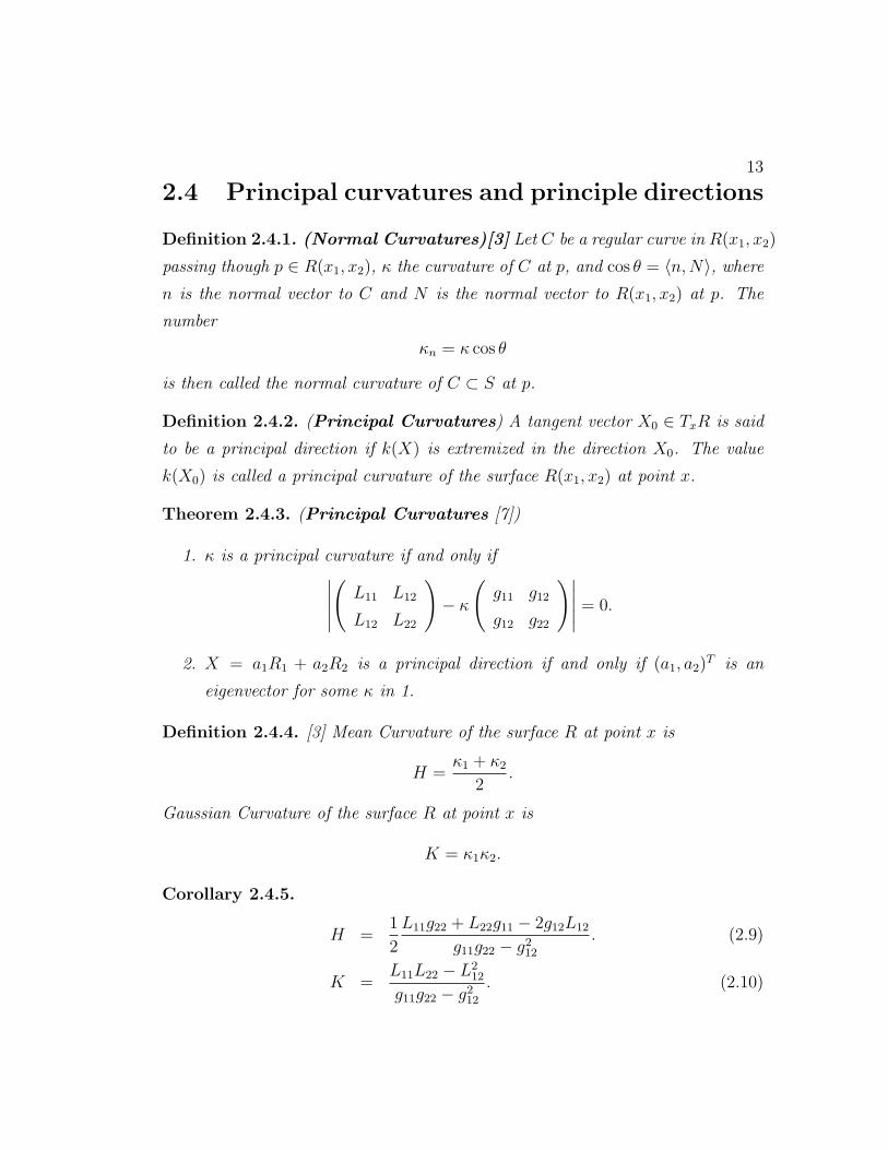
Theorem 2.4.3. (Principal Curvatures [7])
1. κ is a principal curvature if and only if∣∣∣∣∣(L11 L12
L12 L22
)− κ
(g11 g12
g12 g22
)∣∣∣∣∣ = 0.
2. X = a1R1 + a2R2 is a principal direction if and only if (a1, a2)T is an
eigenvector for some κ in 1.
Definition 2.4.4. [3] Mean Curvature of the surface R at point x is
H =κ1 + κ2
2.
Gaussian Curvature of the surface R at point x is
K = κ1κ2.
Corollary 2.4.5.
H =1
2
L11g22 + L22g11 − 2g12L12
g11g22 − g212. (2.9)
K =L11L22 − L2
12
g11g22 − g212. (2.10)

14
Definition 2.4.6. If at x0 ∈ R, κ1 = κ2, then x0 is called an umbilical point of
R; in particular, the planar points (κ1 = κ2 = 0) are umbilical points.
Definition 2.4.7. A regular curve c(t) on a surface R(x1, x2) is called a line of
curvature if c′(t)/|c′(t)| is a principal direction for all t.
Lemma 2.4.8. [3] Let R : Ω→ R3 be a surface, x0 ∈ R is not an umbilical point,
then there exists a neighborhood U0 of x0 and a change of variable ϕ : V0 → U0
such that the coordinate lines of U = U ϕ are lines of curvatures.
Such coordinates are called principal curvature coordinates.
Theorem 2.4.9. [3] If U : Ω→ R3 satisfies g12 = L12 = 0, then U is a principal
curvature coordinates.
Corollary 2.4.10. [3] Under the principal curvature coordinates, the principal
curvatures are
κ1 =L11
g11, κ2 =
L22
g22.
Corollary 2.4.11. Under the principal curvature coordinates (xi)i=1,2,
Λ111 =3κ12
∂g11∂x1
+ g11∂κ1∂x1
, Λ222 =3κ22
∂g22∂x2
+ g22∂κ2∂x2
,
Λ221 = Λ122 = Λ212 =1
2
∂g22∂x1
κ2 =3κ12
∂g11∂x2
+ g11∂κ1∂x2
,
Λ121 = Λ211 = Λ112 =1
2
∂g11∂x2
κ1 =3κ22
∂g22∂x1
+ g22∂κ2∂x1
.
Proof. By Theorem 2.4.9, g12 = L12 = 0, then
Λ111 =∂L11
∂x1+ Γ1
11L11 =∂g11κ1∂x1
+1
2g11
∂g11∂x1
g11κ1 =3κ12
∂g11∂x1
+ g11∂κ1∂x1
,
Λ222 =∂L22
∂x2+ Γ1
22L22 =3κ22
∂g11∂x1
+ g22∂κ2∂x2
,
Λ122 =∂L12
∂x2+ Γ2
12L22 =1
2
∂g22∂x1
κ2 =3κ12
∂g11∂x2
+ g11∂κ1∂x2
,
Λ121 =∂L21
∂x1+ Γ1
12L11 =1
2
∂g11∂x2
κ1 =3κ12
∂g11∂x2
+ g11∂κ1∂x2
.
15
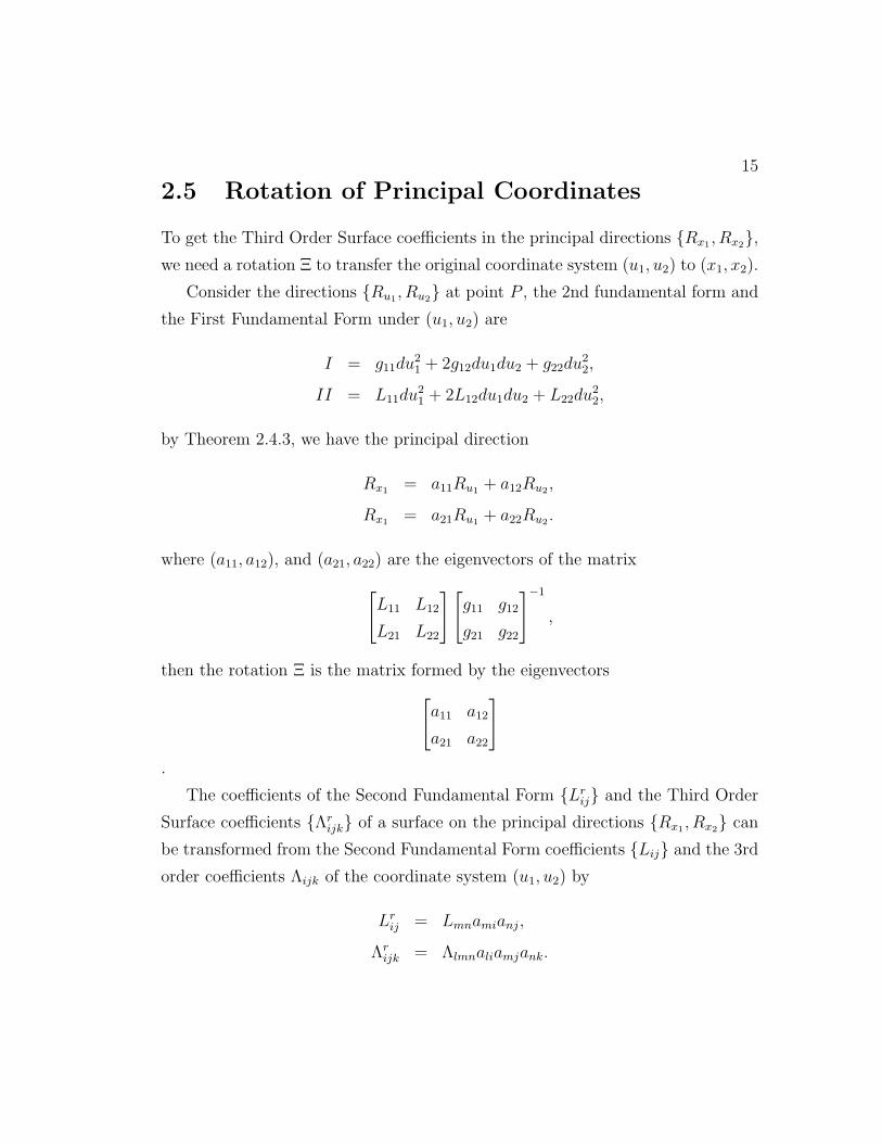
2.5 Rotation of Principal Coordinates
To get the Third Order Surface coefficients in the principal directions Rx1 , Rx2,we need a rotation Ξ to transfer the original coordinate system (u1, u2) to (x1, x2).
Consider the directions Ru1 , Ru2 at point P , the 2nd fundamental form and
the First Fundamental Form under (u1, u2) are
I = g11du21 + 2g12du1du2 + g22du
22,
II = L11du21 + 2L12du1du2 + L22du
22,
by Theorem 2.4.3, we have the principal direction
Rx1 = a11Ru1 + a12Ru2 ,
Rx1 = a21Ru1 + a22Ru2 .
where (a11, a12), and (a21, a22) are the eigenvectors of the matrix[L11 L12
L21 L22
][g11 g12
g21 g22
]−1
,
then the rotation Ξ is the matrix formed by the eigenvectors[a11 a12
a21 a22
].
The coefficients of the Second Fundamental Form Lrij and the Third Order
Surface coefficients Λrijk of a surface on the principal directions Rx1 , Rx2 can
be transformed from the Second Fundamental Form coefficients Lij and the 3rd
order coefficients Λijk of the coordinate system (u1, u2) by
Lrij = Lmnamianj,
Λrijk = Λlmnaliamjank.

Chapter 3
Geometric Optics and Lens
Design
3.1 Geometric optics principles
Design and analysis of ophthalmic lens uses numerical calculation based upon
geometric optics principles. The geometric optics model is sufficient to describe
the properties of an image formed by a lens.
Geometric optics is based on the fundamental assumption that light propagates
along rays. Fermat’s Principle, known as the principle of the shortest optical path,
states that each ray through an optical system follows the path of the shortest
time from points in the object space to points located in the image space. Rays
in a homogeneous medium follow straight lines.
The velocity of propagation of a light ray in a homogeneous isotropic medium
is given by
v =c
n
where c is the velocity of light in vacuum (3.0 × 10⁸ m/s) and n is the index of
refraction of the medium. The length of time of for a ray to propagate from point
16

17
P in object space to point P ′ in the image space is
t =1
c
∫n(s)ds
where s is the length along all the ray vector from P to P ′.
Fermat’s principle can be derived from Huygens’ principle, and can be used to
derive Snell’s law of refraction, which is a formula used to describe the relationship
between the angles of incidence and refraction.
αi
αr
n1
n2
Figure 3.1: Snell’s Law
Lemma 3.1.1 (Snell’s Law).
sinαi
sinαr
=n1
n2
,
where αi, αr are the incident and refraction angles. n1, n2 are the index of re-
fraction of the two media as shown in Figure 3.1.
Lemma 3.1.2. As shown in figure 3.2, let Q be the incident direction, S be the
normal direction at the intersection point, Q′ be the refraction direction, by Snell’s
law,
Q′ = µQ+ γS,
where µ = n1
n2, γ = cosαr − µ cosαi.

18
Q
SQ′
n1
n2
Figure 3.2: The refracted direction
3.2 Characterizing lens performance with a wave-
front
The main characteristics of ophthalmic lenses are power of refraction and astig-
matism. The method for characterizing these properties are based on wavefronts,
and it could be extended to describing properties of lens with arbitrary surfaces.
Consider a point light source that is switched on and off at the time t0. At the
time t > t0 the photons emitted at t0 form a surfaceWt, the wavefront. The shape
of the wavefrontWt changes as it propagates, whether the medium is homogeneous
or inhomogeneous and when it is refracted by a surface.
We characterize the wavefront as a time-dependent surface Wt(x1, x2). Then
we are interested in the local curvatures ofWt along a particular light rayQt0(x01, x
02) :
t→ Wt(x01, x
02). Consider a point at infinity viewed by eye. The point emit a ray
Qt0 , with a planar wavefront Wt. After the wavefront is refracted by the lens sur-
face, it arrives at the back side of the lens at time t = t1. The principal curvature
κ1 and κ2 of the refracted wavefront W ′t1
defines the power of refraction P and
astigmatism A of the lens along the viewing direction (as shown in figure 3.3):
P =κ1 + κ2
2,
A = |κ1 − κ2|.

19
We can write
P = H, A =√H2 −K,
where H and K are mean curvature and Gaussian curvature of the wavefront.
The higher order aberrations such as Comma, Spherical Abberation, etc., can
also be calculated from properties of the wavefront. They depend on a higher
derivatives of the wavefront surface.
κ1
κ2
O′
O
Q′
A
Figure 3.3: Wavefront Curvature Representation
3.3 Wavefront aberration and Zernike polyno-
mials
The deviation of the refracted wavefront after a lens from a desired perfect spher-
ical wavefront is called the wavefront aberration or wavefront distortion.
Consider an orthonormal basis e′′1, e′′2, e′′3, where e′′1 = (0,1,0)×(−θ)
|(0,1,0)×(−θ)| , e′′3 = −θ,
and e′′2 = e′′1 × e′′3. With the origin O′′, let X ′′i be the cartesian coordinates with
20
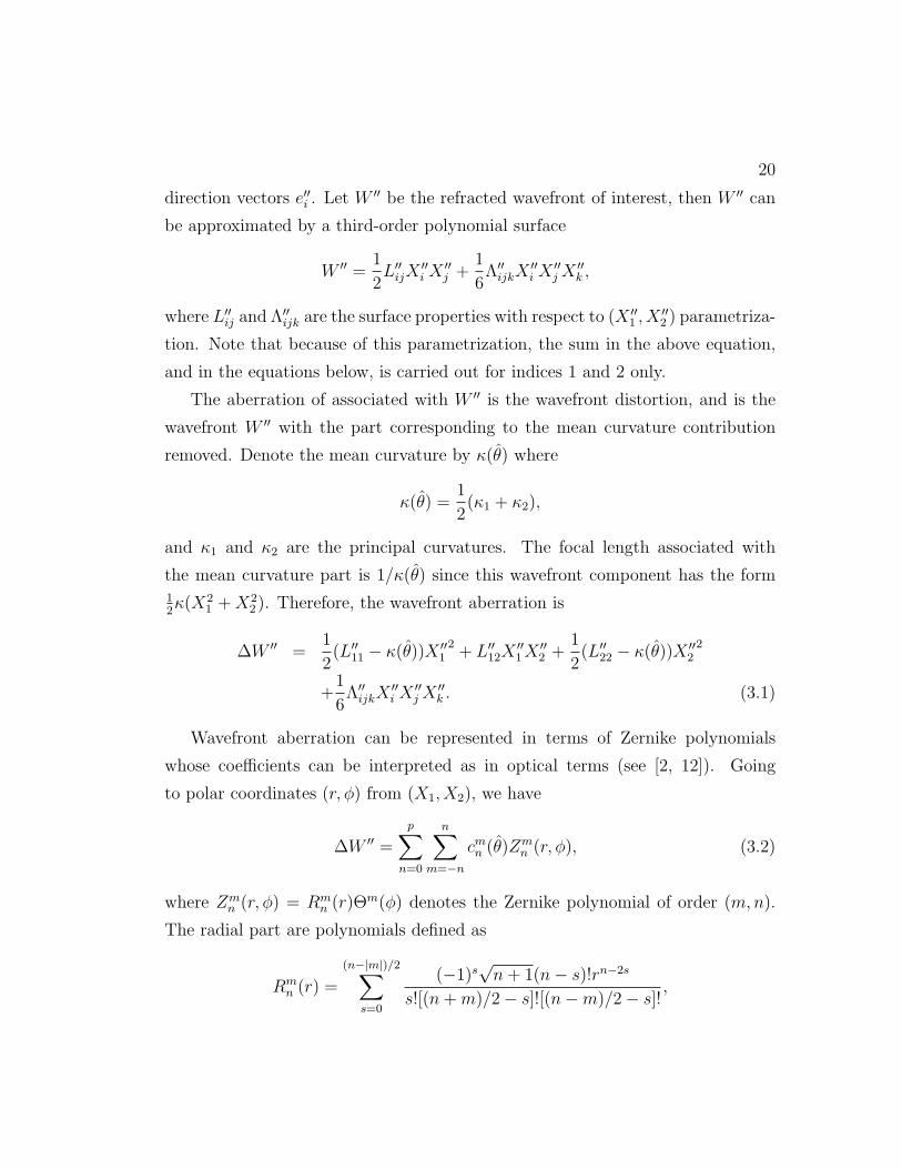
direction vectors e′′i . Let W′′ be the refracted wavefront of interest, then W ′′ can
be approximated by a third-order polynomial surface
W ′′ =1
2L′′
ijX′′i X
′′j +
1
6Λ′′
ijkX′′i X
′′jX
′′k ,
where L′′ij and Λ′′
ijk are the surface properties with respect to (X ′′1 , X
′′2 ) parametriza-
tion. Note that because of this parametrization, the sum in the above equation,
and in the equations below, is carried out for indices 1 and 2 only.
The aberration of associated with W ′′ is the wavefront distortion, and is the
wavefront W ′′ with the part corresponding to the mean curvature contribution
removed. Denote the mean curvature by κ(θ) where
κ(θ) =1
2(κ1 + κ2),
and κ1 and κ2 are the principal curvatures. The focal length associated with
the mean curvature part is 1/κ(θ) since this wavefront component has the form12κ(X2
1 +X22 ). Therefore, the wavefront aberration is
∆W ′′ =1
2(L′′
11 − κ(θ))X ′′12+ L′′
12X′′1X
′′2 +
1
2(L′′
22 − κ(θ))X ′′22
+1
6Λ′′
ijkX′′i X
′′jX
′′k . (3.1)
Wavefront aberration can be represented in terms of Zernike polynomials
whose coefficients can be interpreted as in optical terms (see [2, 12]). Going
to polar coordinates (r, ϕ) from (X1, X2), we have
∆W ′′ =
p∑n=0
n∑m=−n
cmn (θ)Zmn (r, ϕ), (3.2)
where Zmn (r, ϕ) = Rm
n (r)Θm(ϕ) denotes the Zernike polynomial of order (m,n).
The radial part are polynomials defined as
Rmn (r) =
(n−|m|)/2∑s=0
(−1)s√n+ 1(n− s)!rn−2s
s![(n+m)/2− s]![(n−m)/2− s]!,
21
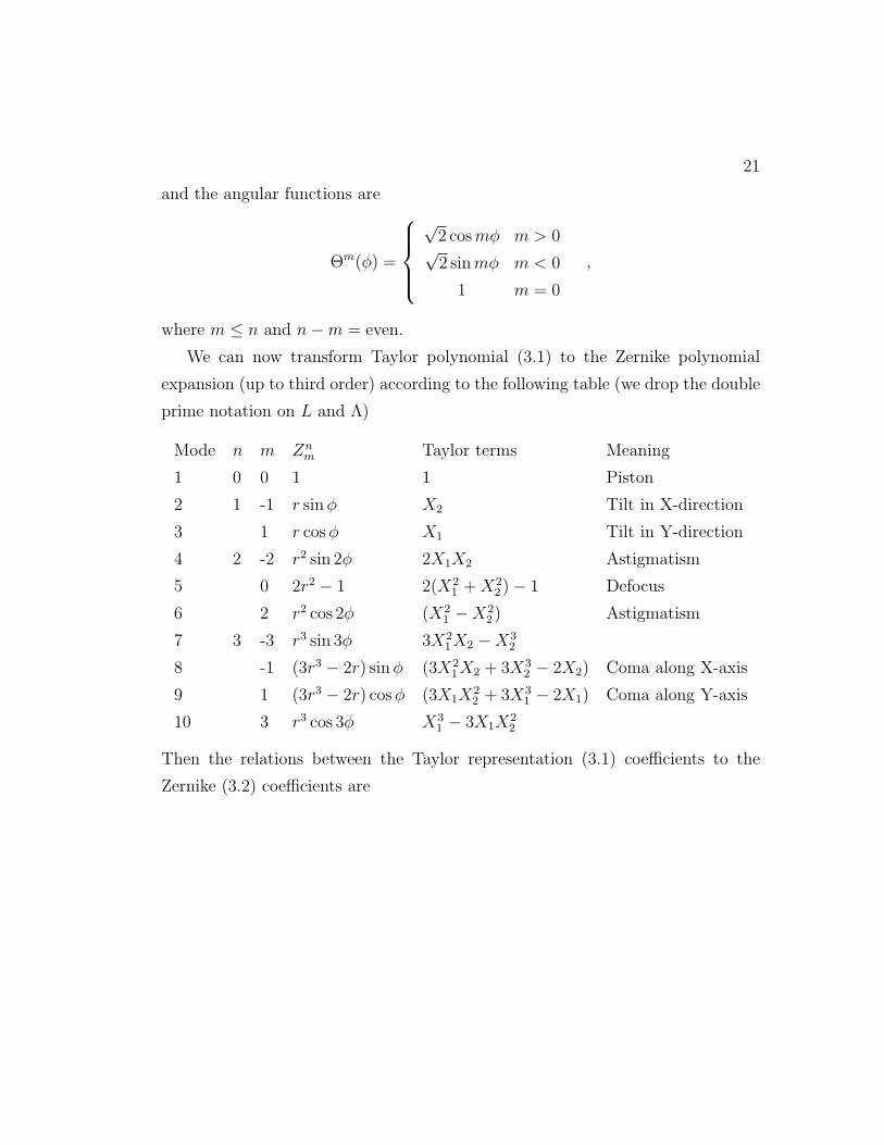
and the angular functions are
Θm(ϕ) =
√2 cosmϕ m > 0√2 sinmϕ m < 0
1 m = 0
,
where m ≤ n and n−m = even.
We can now transform Taylor polynomial (3.1) to the Zernike polynomial
expansion (up to third order) according to the following table (we drop the double
prime notation on L and Λ)
Mode n m Znm Taylor terms Meaning
1 0 0 1 1 Piston
2 1 -1 r sinϕ X2 Tilt in X-direction
3 1 r cosϕ X1 Tilt in Y-direction
4 2 -2 r2 sin 2ϕ 2X1X2 Astigmatism
5 0 2r2 − 1 2(X21 +X2
2 )− 1 Defocus
6 2 r2 cos 2ϕ (X21 −X2
2 ) Astigmatism
7 3 -3 r3 sin 3ϕ 3X21X2 −X3
2
8 -1 (3r3 − 2r) sinϕ (3X21X2 + 3X3
2 − 2X2) Coma along X-axis
9 1 (3r3 − 2r) cosϕ (3X1X22 + 3X3
1 − 2X1) Coma along Y-axis
10 3 r3 cos 3ϕ X31 − 3X1X
22
Then the relations between the Taylor representation (3.1) coefficients to the
Zernike (3.2) coefficients are
22
Mode Zernike coefficients
1 C00 = 1
4(L11 + L22)
2 C1−1 =
112(Λ112 + Λ222)
3 C11 = 1
12(Λ111 + Λ122)
4 C2−2 =
12L12
5 C20 = 1
8(L11 + L22 − 2κ)
6 C22 = 1
2(L11 − L22)
7 C3−3 =
124(3Λ112 − Λ222)
8 C3−1 =
124(Λ112 + Λ222)
9 C31 = 1
24(Λ111 + Λ122)
10 C33 = 1
24(Λ111 − 3Λ122)
3.4 Lens design problem
Plane Wave W
P
O
O′′
W ′′
Z
Y
O
X − Y
Plane Wave W
X
θ θ
O′′
O′
PO′
R1
R2
R2
R1
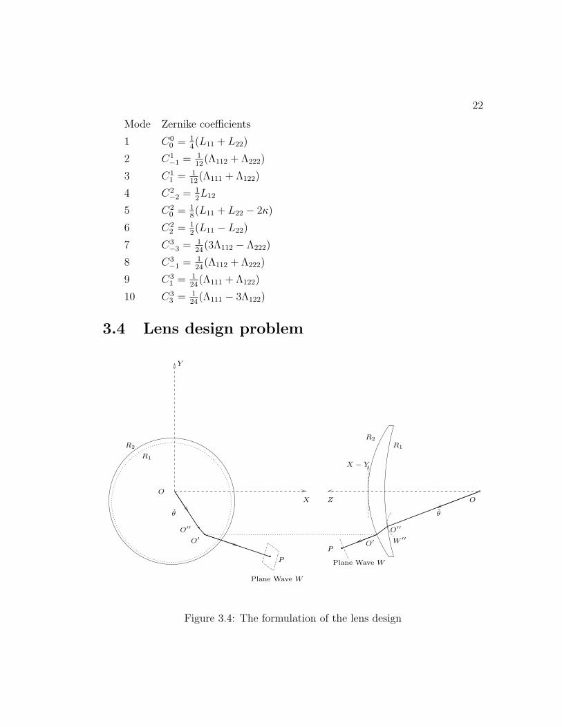
Figure 3.4: The formulation of the lens design

23
As shown in Figure 3.4, let the gaze direction of the eye is θ, the lens surfaces
are R1 and R2, the index of refraction of the lens is n while that of air is 1. To
obtain the diffractive properties of the lens at that gaze direction, we need to
follow the ray at angle θ out from the eye side. A planar wavefront W is set
up at point P with the normal direction Q′ along the ray, then W follows this
direction as it goes back through the lens, generating a refracted wavefront W ′′
at point O′′ at where the ray exits the lens toward the eye. For any θ ∈ Ω, we
can calculate the Second Fundamental Form coefficients L(θ) and Third Order
Surface coefficients Λ(θ) of W ′′. In the next chapter, we will outline how one can
calculate a wavefront after refraction by a single surface. Therefore, in principle,
we can perform such a calculation twice in order to calculate how a wavefront is
diffracted by a lens.
Therefore, for a given lens with two lens surfaces R1 and R2 and a given gaze
direction θ, we can calculate the Zernike coefficients cij(θ) and lens power, which
is defined as the mean curvature κ(θ).
The Progressive Additional Lens (PAL) design problem is described as follows.
We want to come close to desired power distribution P (θ) over a set of gaze
directions Ω. The aberrations in all these directions should also be minimized as
well. Therefore, the target functional we want to optimize is
J (R1, R2) =
∫Ω
β|κ(θ)− P (θ)|2dθ +∫Ω
∑i
∑j
αij(c
ij(θ))
2dθ. (3.3)
The weight αij and β are θ dependent and represents the importance of aberration
and closeness to desired power in the gaze direction θ.
In most PAL design, only one surface, either the front or the back, is designed
for progressive power correction. The other surface is typically sphere or toric,
depending on whether the wearer has prescribed astigmatism correction. The
functional above could be considered with one of the surfaces fixed. The resulting
design problem is to find the other surface that minimizes the functional. One
could consider designing both surfaces at the same time although the need to
make sure that the surfaces do not intersect must be enforced by a constraint.

Chapter 4
Wavefront deformation through
smooth refracting lens surface
4.1 Wavefront tracing through optical system
In order to understand how light propagates through a lens, we must first under-
stand how it interacts with a single interface. To do so, we consider the geometrical
optics approximation where light travel along rays, and optical energy along rays
with the same phase form a wavefront.
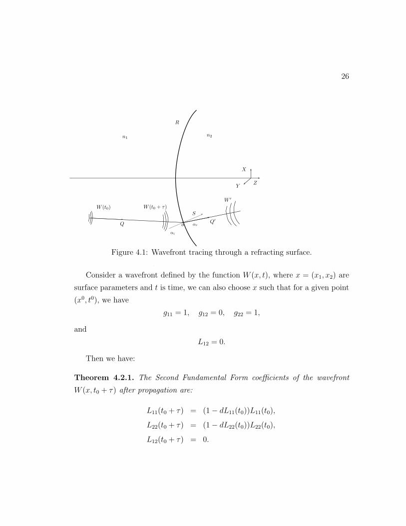
Figure 4.1 shows a brief description of wavefront tracing through a refracting
surface. Consider a wavefront in three-dimensional space defined by the vector
function W (x, t), where x = (x1, x2) are surface parameters and t is time. Denote
W (x, t0) as the initial wavefront. Then W (x, t0 + τ) is the wavefront after time
τ . Let Q(x) be the unit normal vector of W (x, t), which does not depend on t in
a homogeneous medium. W (x, t) strikes a refracting surface R(x) at x = (x1, x2)
with unit normal S(x), giving rise to a refracted wavefront W ′(x′, t) at x′ =
(x′1, x′2), with unit normal Q′(x′). Here it is assumed that the index of refraction
of the media are constant and equal to n1 and n2, the angle of incidence is αi and
the angle of refraction is αr.
24

25
The corresponding equation can be obtained by considering the physical pro-
cess: Let T (x) be the travel time between W (x, t) along a ray in the direction
Q(x) and the point O on R. Let L be the total time in which W (x, t) travels to
W ′, then
R =W + c1TQ, (4.1a)
W ′ =W + c1TQ+ c2(L− T )Q′, (4.1b)
which imply
W + c1TQ = R = W ′ − c2(L− T )Q′, (4.2)
where c1 = c/n1, c2 = c/n2 are the light speeds in the corresponding media.
We can denote cT = ϕ, where c is the light speed in vacuum, then the equation
is now
W + µ1ϕ ·Q = R =W ′ − µ2(cL− ϕ) ·Q′, (4.3)
where µ1 =c1cand µ2 =
c2c.
When a wavefront passes through an optical system, as described above, two
phenomena are responsible for transforming the curvature of the wavefront:
1. Propagation in a homogenous medium.
2. Refraction at an optical boundary.
In the following sections, we will derive formulas for the Second Fundamental
Form coefficients and the third-order surface coefficients after the wavefront has
gone through the surface R.
4.2 J. Kneisly’s Approach
In J. Kneisly’s paper [8], he propose a formula of the Second Fundamental Form
of the wavefront under propagation.
26
n1n2
R
Z
X
Y
Q
S
αi
αr
Q′
W (t0) W (t0 + τ)
W ′
*
o
Figure 4.1: Wavefront tracing through a refracting surface.
Consider a wavefront defined by the function W (x, t), where x = (x1, x2) are
surface parameters and t is time, we can also choose x such that for a given point
(x0, t0), we have
g11 = 1, g12 = 0, g22 = 1,
and
L12 = 0.
Then we have:
Theorem 4.2.1. The Second Fundamental Form coefficients of the wavefront
W (x, t0 + τ) after propagation are:
L11(t0 + τ) = (1− dL11(t0))L11(t0),
L22(t0 + τ) = (1− dL22(t0))L22(t0),
L12(t0 + τ) = 0.

27
In particular, the principal curvatures evolve as
κ1(t0 + τ) =κ1(t0)
1− dκ1(t0), κ2(t0 + τ) =
κ2(t0)
1− dκ2(t0).
where d = cτ the distance W traveled during time τ .
In [8], J. Kneisly also proposed a formula of representing Second Fundamental
Form of the refracted wavefront by the coefficients of the initial wavefront and the
refracting lens surface.
Consider point O where three surfaces meet, then
O =W (x01, x02) = R(x01, x
02) = W ′(x′01 , x
′02 ),
Snell’s law gives the relation between the normal vectors Q′ and Q, S.
Q′(x′01 , x′02 ) = µQ(x01, x
02) + γS(x01, x
02),
where γ = cosαr − µ cosαi, where αi and αr are the angles of incidence and
refraction, respectively, µ = n1/n2 = c1/c1 is the ratio of refraction.
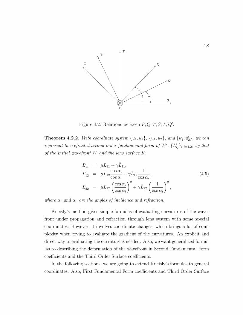
By the law of refraction, the normals Q,S,Q′ are all coplanar. Define
P = (Q× S)/|Q× S| = (Q× S)/ sinαi,
which is perpendicular to the plane of refraction and tangent to all the surfaces.
Let T = Q × P, T = S × P , and T ′ = Q′ × P , which are tangent to the
corresponding surfaces, respectively, and lie in the plane of refraction, as shown in
Figure 4.2. Then we can select coordinates system of (u1, u2) such that at point
O, we have
P =Wu1 , T =Wu2 ,
P = Ru1 , T = Ru2 , (4.4)
P =W ′u′1, T ′ = W ′
u′2,
28
Q’
T’
S
P
T
T
Q
αi
αr
Figure 4.2: Relations between P,Q, T, S, T , Q′.
Theorem 4.2.2. With coordinate system u1, u2, u1, u2, and u′1, u′2, we can
represent the refracted second order fundamental form of W ′, L′iji,j=1,2, by that
of the initial wavefront W and the lens surface R:
L′11 = µL11 + γL11,
L′12 = µL12
cosαi
cosαi
+ γL121
cosαr
, (4.5)
L′22 = µL22
(cosαi
cosαi
)2
+ γL22
(1
cosαi
)2
,
where αi and αr are the angles of incidence and refraction.
Kneisly’s method gives simple formulas of evaluating curvatures of the wave-
front under propagation and refraction through lens system with some special
coordinates. However, it involves coordinate changes, which brings a lot of com-
plexity when trying to evaluate the gradient of the curvatures. An explicit and
direct way to evaluating the curvature is needed. Also, we want generalized formu-
las to describing the deformation of the wavefront in Second Fundamental Form
coefficients and the Third Order Surface coefficients.
In the following sections, we are going to extend Kneisly’s formulas to general
coordinates. Also, First Fundamental Form coefficients and Third Order Surface
29
coefficients on propagation and on refraction under general coordinates are also
presented. Note that all the equations are carried out for indices 1 and 2 only.
4.3 Wavefront surface coefficients on propaga-
tion
4.3.1 The Second Fundamental Form coefficients on prop-
agation
Let v be the local speed of light in a homogenous medium, then
W (x, t0 + τ) =W (x, t0) + τvQ(x), and Wt = vQ,
where τ is the travel time.
Let d = τv be the distance light traveled during time τ , then take the first
derivative on xi, we have
Wxi(t0 + τ) = Wxi
(t0) + dQi.
By the equation of Weingarten (2.4),
Qi = −gkj(t0)Lji(t0)Wk(t0),
then
Wxi(t0 + τ) = Wxi
(t0)− dgkj(t0)Lji(t0)Wxk(t0). (4.6)
Therefore, by definition of gij
gij(t0 + τ) = ⟨Wxi(t0 + τ),Wxj
(t0 + τ)⟩,
by (4.6),
gij(t0+ τ) = ⟨Wxi(t0)−dgkl(t0)Lli(t0)Wxk
(t0),Wxj(t0)−dgnm(t0)Lmj(t0)Wxn(t0)⟩.
30
Expanding this equation gives
gij(t0 + τ) = gij(t0)− dgnm(t0)gin(t0)Lmj(t0)− dgkl(t0)gkj(t0)Lli(t0)
+d2gkl(t0)gnm(t0)gkn(t0)Lli(t0)Lmj(t0). (4.7)
Similarly, by the definition of Lij,
Lij(t0 + τ) = −⟨Wxi(t0 + τ), Qxj
⟩,
Expanding the expression gives
Lij(t0 + τ) = Lij(t0)− dgkj(t0)Lji(t0)Lkj(t0),
which is
Lij(t0 + τ) = (1− dgkj(t0)Lkj(t0))Lij(t0).
Theorem 4.3.1. The Second Fundamental Form coefficients on propagation is
given by
Lij(t0 + τ) = (1− dgkjLkj(t0))Lij(t0),
where d is the distance the wavefront propagates during time τ . In particular,
under unit orthogonal coordinate system, where g11 = g12 = 1 and g12 = 0, L(t0 +
τ) have representations,
L11(t0 + τ) = (1− dL11(t0))L11(t0),
L22(t0 + τ) = (1− dL22(t0))L22(t0),
L12(t0 + τ) = L21(t0 + τ) = 0.
Corollary 4.3.2. The principal curvature of the wavefront on propagation is given
by
κi(t0 + τ) =κi(t0)
1− dκi(t0),
where d is the distance the wavefront propagates during time τ .
31
Corollary 4.3.3. Mean curvature and Gaussian Curvature of the wavefront on
propagation is given by
H(t0 + τ) =H(t0)− dK(t0)
1− 2dH(t0) + d2K(t0)
K(t0 + τ) =K(t0)
1− 2dH(t0) + d2K(t0)
Proof. By definition 2.4.5,
H(t0 + τ) =1
2(κ1(t0 + τ) + κ2(t0 + τ)),
By Corollary 4.3.2
H(t0 + τ) =1
2
(κ1(t0)
1− dκ1(t0)+
κ2(t0)
1− dκ2(t0)
).
Combine these two fractions, we obtain
H(t0 + τ) =1
2
κ1(t0) + κ2(t0)− 2dκ1(t0)κ2(t0))
1− d(κ1(t0) + κ2(t0)) + d2κ1(t0)κ2(t0).
At the end, applying the definition of H(t0) and K(t0), we have
H(t0 + τ) =H(t0)− dK(t0)
1− 2dH(t0) + d2K(t0). (4.8)
Similarly, we have
K(t0 + τ) =K(t0)
1− 2dH(t0) + d2K(t0). (4.9)
Definition 4.3.4. The astigmatism (or local cylinder) A of a wavefront is defined
as
A =√H2 −K = |κ1 − κ2|, (4.10)
where κ1, κ2 are principal curvatures of the wavefront.

32
Corollary 4.3.5. The astigmatism A of the wavefront on propagation is given by
A(t0 + τ) =A(t0)
1− 2dH(t0) + d2K(t0)
Proof. By definition 4.3.4,
A2(t0 + τ) = H2(t0 + τ)−K(t0 + τ).
By Corollary 4.3.3, expanding H(t0 + τ) and K(t0 + τ) gives
A2(t0 + τ) = (H(t0)− dK(t0)
1− 2dH(t0) + d2K(t0))2 − K(t0)
1− 2dH(t0) + d2K(t0).
Combining the expression gives
A(t0 + τ) =(H(t0)− dK(t0))
2 −K(t0)(1− 2dH(t0) + d2K(t0))
(1− 2dH(t0) + d2K(t0))2.
Hence,
A2(t0 + τ) =H(t0)
2 −K(t0)
(1− 2dH(t0) + d2K(t0))2.
By the definition of A(t0) =√H(t0)2 −K(t0),
A2(t0 + τ) =(A(t0))
2
(1− 2dH(t0) + d2K(t0))2,
then, A(t0 + τ) =A(t0)
1− 2dH(t0) + d2K(t0).
4.3.2 The Third Order Surface coefficients on propagation
By definition (2.3.1),
Λijk(t0 + τ) = −⟨Wxixj(t0 + τ), Qxk
⟩ − ⟨Wxixk(t0 + τ), Qxj
⟩
−⟨Wxi(t0 + τ), Qxjxk
⟩.
Since
Wxixj(t0 + τ) =Wxixj
(t0) + dQxixj,

33
then
Λijk(t0 + τ) = −⟨Wxixj(t0) + dQxixj
, Qxk⟩ − ⟨Wxixk
(t0) + dQxixk, Qxj⟩
− ⟨Wxi(t0) + dQxi
, Qxjxk⟩.
Also,
Λijk(t0) = −⟨Wxixj(t0), Qxk
⟩ − ⟨Wxixk(t0), Qxj
⟩ − ⟨Wxi(t0), Qxjxk
⟩.
We have
Λijk(t0 + τ) = Λijk(t0)− d(⟨Qxixj, Qxk
⟩+ ⟨Qxixk, Qxj⟩+ ⟨Qxjxk
, Qxi⟩).
With lemma 2.3.3,
⟨Qxixj, Qxk
⟩ = ⟨∆lijRxl
, Qxk⟩ = −∆l
ijLlk.
Overall, we have the formula describing the Third Order Surface coefficients
on propagation.
Theorem 4.3.6. The Third Order Surface coefficients on propagation are given
by
Λijk(t0 + τ) = Λijk(t0) + d[∆lik(t0)Llj(t0) + ∆l
jk(t0)Lli(t0)
+∆lij(t0)Llk)(t0)],
where d is the distance the wavefront propagates during time τ .
4.4 Wavefront surface coefficients on refraction
4.4.1 The derivative of ϕ
Recall equation (4.3), if we assume that µ1 = 1 and µ2 = µ, then
W + ϕQ = R = W ′ − µ(l − ϕ)Q′.

34
Since at the strike point O,
O =W (x01, x02) = R(x01, x
02) = W ′(x′01 , x
′02 ),
then ϕ = 0 at point O, and l = 0 for this refracted wavefront W ′.
Lemma 4.4.1.
W ′xi=Wxi
+ ϕxi(Q− µQ′) = Rxi
− µϕxiQ′,
where
ϕxi=⟨Rxi
, Q′⟩µ
= ⟨Rxi, Q⟩.
Proof. First differentiation on x gives
Wxi+ ϕxi
Q = Rxi= W ′
xi+ µϕxi
Q′.
Then we apply inner product with S through both sides, since W ′xi·Q′ = 0,
ϕxi=⟨Rxi
, Q′⟩µ
.
and⟨Rxi
, Q′⟩µ
=⟨Rxi
, (µQ+ γS)⟩µ
= ⟨Rxi, Q⟩.
Lemma 4.4.2.
W ′xixj
= Wxixj+ ϕxixj
(Q− µQ′) + ϕxi(Qxj
− µQ′xj) + ϕxj
(Qxi− µQ′
xi)
= Rxixj− µϕxixj
Q′ − µϕxiQ′
xj− µϕxj
Q′xi
where
ϕxixj=⟨Rxixj
, Q′⟩µ
−LW ′ij
µ= ⟨Rxixj
, Q⟩+ LWij .

35
Proof. Taking derivative of equation 4.3 with respect to xi twice, we have
Rxixj= Wxixj
+ ϕxixjQ+ ϕxi
Qxj+ ϕxj
Qxi
= W ′xixj
+ µϕxixjQ′ + µϕxi
Q′xj+ µϕxj
Q′xi.
Since ⟨Q′xi, Q′⟩ = 0, then
⟨W ′xixj
, Q′⟩ = ⟨Rxixj, Q′⟩ − ϕxixj
.
Then,
ϕxixj=⟨Rxixj
, Q′⟩µ
−LW ′
ij
µ.
By lemma 3.1.2,
Q′ = µQ+ γS,
where γ = cosαr − µ cosαi, then
⟨Rxixj, Q′⟩ = ⟨Rxixj
, µQ+ γS⟩ = µ⟨Rxixj, Q⟩+ γ⟨Rxixj
, S⟩.
Recall that ⟨Rxixj, S⟩ = LR
ij, we have
ϕxixj=⟨Rxixj
, µQ⟩µ
+ γLR
ij
µ−LW ′ij
µ.
By theorem 4.4.4,
LWij =
LW ′ij
µ− γ
LRij
µ,
then ϕxixjis
ϕxixj= ⟨Rxixj
, Q⟩+ LWij .
36
4.4.2 The Fundamental Form coefficients on refraction
We are now ready to derive the First Fundamental Form coefficients and the
Second Fundamental Form coefficients of the refracted wavefront.
Theorem 4.4.3. The First Fundamental Form coefficients gW′of W ′ under co-
ordinate system xi2i=1 are
gW′
ij = gRij − µ2ϕxiϕxj
= gWij − (2− µ2)ϕxiϕxj
.
Proof. By definition 2.1,
gW′
ij = ⟨W ′xi,W ′
xj⟩.
According to lemma 4.4.1,
W ′xi= Rxi
− ϕxiµQ′,
then
gW′
ij = ⟨Rxi− ϕxi
µQ′, Rxj− ϕxj
µQ′⟩.
Expanding the above expression gives
gW′
ij = ⟨Rxi, Rxj⟩ − µϕxi
⟨Rxj, Q′⟩ − µϕxj
⟨Rxi, Q′⟩ − µ2ϕxi
ϕxj. (4.11)
By the definition of gRij , we have
⟨Rxi, Rxj⟩ = gRij .
Also
⟨Rxi, Q′⟩ = ⟨Rxj
, µQ+ γS⟩ = µ⟨Rxj, Q⟩+ γ⟨Rxj
, S⟩.
Recall lemma 4.4.1,
ϕxi= ⟨Rxi
, Q′⟩/µ.
Then the third term of equation (4.11) turns out to be
−µϕxj⟨Rxi
, Q′⟩ = −µϕxj(µϕxi
) = −µ2ϕxiϕxj
.

37
Overall, we have
gW′
ij = gRij + µ2ϕxiϕxj− µϕxi
ϕxj− µϕxj
ϕxi
= gRij − µ2ϕxiϕxj
.
Theorem 4.4.4. The Second Fundamental Form coefficients LW ′of W ′ under
coordinate system xi2i=1 are
LW ′
ij = µLWij + γLR
ij.
Proof. By definition 2.2,
LW ′
ij = ⟨W ′xixj
, Q′⟩.
Expanding Q′ gives
LW ′
ij = ⟨W ′xixj
, µQ+ γS⟩ = µ⟨W ′xixj
, Q⟩+ γ⟨W ′xixj
, S⟩.
By lemma 4.4.2,
⟨W ′xixj
, Q⟩ = ⟨Wxixj+ ϕxixj
(Q− µQ′) + ϕxi(Qxj
− µQ′xj) + ϕxj
(Qxi− µQ′
xi), Q⟩,
and
⟨W ′xixj
, S⟩ = ⟨Rxixj− ϕxixj
µQ′ − ϕxiµQ′
xj− ϕxj
µQ′xi, S⟩.
Expanding the equations gives
⟨W ′xixj
, Q⟩ = ⟨Wxixj, Q⟩+ ϕxixj
⟨(Q− µQ′), Q⟩+ ϕxi⟨(Qxj
− µQ′xj), Q⟩
+ϕxj⟨(Qxi
− µQ′xi), Q⟩,
and
⟨W ′xixj
, S⟩ = ⟨Rxixj, S⟩ − ϕxixj
⟨µQ′, S⟩ − ϕxi⟨µQ′
xj, S⟩ − ϕxj
⟨µQ′xi, S⟩.
Recall that
⟨Wxixj, Q⟩ = LW
ij , ⟨Qxi, Q⟩ = 1,
38
then
⟨W ′xixj
, Q⟩ = LWij + ϕxixj
− µϕxixj⟨Q′, Q⟩ − µϕxi
⟨Q′xj, Q⟩ − µϕxj
⟨Q′xi, Q⟩,
Also
⟨Rxixj, S⟩ = LR
ij,
we have
⟨W ′xixj
, S⟩ = LRij − µϕxixj
⟨Q′, S⟩ − µϕxi⟨Q′
xj, S⟩ − µϕxj
⟨Q′xi, S⟩.
Combining them gives
LW ′
ij = µ(LWij + ϕxixj
− µϕxixj⟨Q′, Q⟩ − µϕxi
⟨Q′xj, Q⟩ − µϕxj
⟨Q′xi, Q⟩)
+γ(LRij − µϕxixj
⟨Q′, S⟩ − µϕxi⟨Q′
xj, S⟩ − µϕxj
⟨Q′xi, S⟩).
Recall that Q′ = µQ+ γS, then
µ2ϕxixj⟨Q′, Q⟩+ γµϕxixj
⟨Q′, S⟩ = µϕxixj⟨Q′, µQ+ γS⟩
= µϕxixj⟨Q′, Q′⟩
= µϕxixj,
given that ⟨Q′, Q′⟩ = 1.
Similarly,
µ2ϕxi⟨Q′
xj, Q⟩+ γµϕxi
⟨Q′xj, S⟩ = µϕxi
⟨Q′xj, Q′⟩,
the expression is eliminated since ⟨Q′xj, Q′⟩ = 0. Similar derivation leads to
µ2ϕxj⟨Q′
xi, Q⟩+ γµϕxj
⟨Q′xi, S⟩ = µϕxj
⟨Q′xi, Q′⟩ = 0.
Overall, we have
LW ′
ij = µLWij + γLR
ij.
39
If we adapter the coordinates in Kneisly’s paper [8], as in equations (4.4),
u1, u2, u1, u2, and u′1, u′2, according to 4.4.4, we have
(LW ′)rij = µ(LW )rmn
∂um∂u′i
∂um∂u′j
+ γ(LR)rmn
∂um∂u′i
∂um∂u′j
.
Recall that
du1 = du1 = du′1, and du2 = cosαidu2 =cosαi
cosαr
du′2,
in particular,∂u′i∂uj
=∂u′i∂uj
= 0, if i = j, then we have
(LW ′)r11 = µ(LW )r11 + γ(LR)r11,
(LW ′)r12 = µ(LW )r12
cosαi
cosαi
+ γ(LR)r121
cosαr
,
(LW ′)r22 = µ(LW )r22
(cosαi
cosαi
)2
+ γ(LR)r22
(1
cosαi
)2
.
Therefore, with coordinate systems u1, u2, u1, u2, and u′1, u′2, our result
coincides with Kneisly’s formula (4.5).
From theorem 4.4.4, the Second Fundamental Form coefficients of the refracted
wavefront W ′ can be fully represented by the Second Fundamental Form coeffi-
cients of the initial wavefront and the refract surface.
Also, by Corollary 2.4.5, we have the direct formula of mean curvature and
Gaussian curvature of the refracted wavefront W ′,
Theorem 4.4.5.
HW ′= µHW ∆W
ΘW
− 1
2
ΠW
ΘW
+ γHR∆R
ΘR
− 1
2
ΠR
ΘR
,
KW ′= µ2KW
∆W
ΘW
+ γ2KR∆R
ΘR
+ µγσ
ΘR
.

40
where
∆W = gW11gW22 − (gW12 )
2;
∆R = gR11gR22 − (gR12)
2;
ΘW = (gW11gW22 − (gW12 )
2)− (2− 2µ2)(ϕxiϕxj
gWij );
ΘR = (gR11gR22 − (gR12)
2)− µ2(ϕxiϕxj
gWij );
ΠW = (2− 2µ2)(ϕxiϕxj
LWij );
ΠR = µ2(ϕxiϕxj
LRij);
σ = LR11L
W22 + LR
11LW22 − 2LR
12LW12 .
Proof. By corollary 2.4.5,
HW ′=
1
2
LW ′11 g
W ′22 + LW ′
22 gW ′11 − 2gW
′12 L
W ′12
gW′
11 gW ′22 − (gW
′12 )2
then by theorem 4.4.4,
LW ′
11 gW ′
22 = (µLW11 + γLR
11)gW ′
22 .
Also by theorem 4.4.3,
LW ′
11 gW ′
22 = µLW11(g
W22 − (2− µ2)ϕ2
x2) + γLR
11(gR22 − µ2ϕ2
x2).
Expanding the above expression gives
LW ′
11 gW ′
22 = µLW11g
W22 − µ(2− µ2)ϕ2
x2LW
11 + γLR11g
R22 − µ2γϕ2
x2LR11.
Similarly, we can deduce that
LW ′
12 gW ′
12 = µLW12g
W12 − µ(2− µ2)ϕx1ϕx2L
W12 + γLR
12gR12 − µ2γϕx1ϕx2L
R12.
and
LW ′
22 gW ′
11 = µLW22g
W11 − µ(2− µ2)ϕ2
x1LW
22 + γLR22g
R11 − µ2γϕ2
x1LR22.
Also, by theorem 4.4.3,
gW′
11 gW ′
22 − (gW′
12 )2 = (gW11 − (2− µ2)ϕ2x1)(gW22 − (2− µ2)ϕ2
x2)− (gW12 − (2− µ2)ϕx1ϕx2)
2.
(4.12)

41
and
gW′
11 gW ′
22 − (gW′
12 )2 = (gR11 − µ2ϕ2x1)(gR22 − µ2ϕ2
x2)− (gR12 − µ2ϕx1ϕx2)
2. (4.13)
Simplifying (4.12) and (4.13) gives
gW′
11 gW ′
22 − (gW′
12 )2 = (gW11gW22 − (gW12 )
2)− (2− 2µ2)(ϕxiϕxj
gWij )
= (gR11gR22 − (gR12)
2)− µ2(ϕxiϕxj
gWij ).
Therefore, we have
HW ′=
1
2
µ(gW11LW22 + gW22L
W11 − 2gW12L
W12)
(gW11gW22 − (gW12 )
2)− (2− 2µ2)(ϕxiϕxj
gWij )
+1
2
(2− 2µ2)(ϕxiϕxj
LWij )
(gW11gW22 − (gW12 )
2)− (2− 2µ2)(ϕxiϕxj
gWij )
+γ1
2
gR11LR22 + gR22L
R11 − 2gR12L
R12)
(gR11gR22 − (gR12)
2)− µ2(ϕxiϕxj
gWij )
+1
2
µ2(ϕxiϕxj
LRij)
(gR11gR22 − (gR12)
2)− µ2(ϕxiϕxj
gWij ).
With the notations defined above, we have
HW ′= µHW ∆W
ΘW
− 1
2
ΠW
ΘW
γHR∆R
ΘR
− 1
2
ΠR
ΘR
.
Similarly, by Corollary 2.4.5,
KW ′=
LW ′11 L
W ′22 − (LW ′
12 )2
gW′
11 gW ′22 − (gW
′12 )2
.
Then by theorem 4.4.4
LW ′
11 LW ′
22 − (LW ′
12 )2 = (µLW
11 + γLR11)(µL
W22 + γLR
22)− (µLW12 + γLR
12)2
Expanding the expression gives
LW ′
11 LW ′
22 − (LW ′
12 )2 = µ2(LW
11LW22 − (LW
12)2) + γ2(LR
11LR22 − (LR
12)2)
−2µγ(LR11L
W22 + LR
11LW22 − 2LR
12LW12).
42
Then
KW ′= µ2 LW
11LW22 − (LW
12)2
(gW11gW22 − (gW12 )
2)− (2− 2µ2)(ϕxiϕxj
gWij )+
γ2LR11L
R22 − (LR
12)2
(gR11gR22 − (gR12)
2)− µ2(ϕxiϕxj
gWij )
+µγLR11L
W22 + LR
11LW22 − 2LR
12LW12
(gR11gR22 − (gR12)
2)− µ2(ϕxiϕxj
gWij ),
which is
KW ′= µ2KW
∆W
ΘW
+ γ2KR∆R
ΘR
+ µγσ
ΘR
.
4.4.3 The Third Order Surface coefficients on refraction
The Third Order Surfaces coefficients of W ′ on refraction involves the derivative
of the traveling distance ϕ, the Second Fundamental Form and the Third Order
Surfaces coefficients of W and R.
Theorem 4.4.6. The Third Order Surface coefficients Λ of W ′ under coordinate
system xi2i=1 are
ΛW ′
ijk = µΛWijk + γΛR
ijk + µ(ΠW ′
ik − ΠWik ) + µϕxj
(ΠW ′
ik − ΠWik ) + µϕxk
(ΠW ′
ik − ΠWik ).
ΠWij is defined as
ΠWij = (gW )lmLW
il LWjm, ΠW ′
ij = (gW′)lmLW ′
il LW ′
hm.
Proof. By definition 2.3.1,
ΛW ′
ijk = ⟨W ′ijk, Q
′⟩.
By Q′ = µQ+ γS,
ΛW ′
ijk = ⟨W ′ijk, (µQ+ γS)⟩.

43
Since
W ′ijk = Wijk + (ϕQ)ijk − (µϕQ′)ijk)
= Rijk − µ(ϕQ′))ijk,
then
ΛW ′
ijk = ⟨(Wijk + (ϕQ)ijk − (µϕQ′)ijk), (µQ)⟩+ ⟨(Rijk − (µϕQ′))ijk, (γS)⟩,
which is
ΛW ′
ijk = µ⟨(Wijk, Q⟩+ γ⟨(Rijk, S⟩+ µ⟨(ϕQ)ijk, Q⟩ − ⟨(µϕQ′)ijk), µQ+ γS⟩.
Notice that
ΛWijk = ⟨(Wijk, Q⟩, ΛR
ijk = ⟨(Rijk, S⟩,
then
ΛW ′
ijk = µΛWijk + γΛR
ijk + µ⟨(ϕQ)ijk, Q⟩
−⟨(µϕQ′)ijk), µQ+ γS⟩.
Expand ⟨(ϕQ)ijk, Q⟩, we have
⟨(ϕQ)ijk, Q⟩ = ⟨ϕQijk, Q⟩+ ⟨ϕiQjk, Q⟩+ ⟨ϕjQik, Q⟩+ ⟨ϕkQij, Q⟩
+⟨ϕijQk, Q⟩+ ⟨ϕikQj, Q⟩+ ⟨ϕjkQi, Q⟩
+⟨ϕijkQ,Q⟩,
Given the fact that at the intersection point,
ϕ = 0,
and Q is an unit normal vector,
⟨Q,Q⟩ = 1, ⟨Qi, Q⟩ = 0,
⟨(ϕQ)ijk, Q⟩ = ⟨ϕiQjk, Q⟩+ ⟨ϕjQik, Q⟩+ ⟨ϕkQij, Q⟩+ ϕijk.

44
By lemma 2.3.3,
⟨Qij, Q⟩ = ⟨(∆kij)
WWk +ΠWij Q,Q⟩ = ΠW
ij ,
where ΠWij = −(gW )lkLW
li LWkj . Therefore,
⟨(ϕQ)ijk, Q⟩ = ϕiΠWjk + ϕjΠ
Wik + ϕkΠ
Wij + ϕijk.
Similarly,
⟨(ϕQ′)ijk, Q′⟩ = ϕiΠ
W ′
jk + ϕjΠW ′
ik + ϕkΠW ′
ij + ϕijk,
where ΠW ′ij = −(gW ′
)lkLW ′
li LW ′
kj .
With all the information, the simplified form of ΛW ′
ijk is
ΛW ′
ijk = µΛWijk + γΛR
ijk + µ(ΠW ′
ik − ΠWik ) + µϕxj
(ΠW ′
ik − ΠWik ) + µϕxk
(ΠW ′
ik − ΠWik ).
From theorem 4.4.6, the Third Order Surface coefficients of the refracted wave-
front W ′ involves the Third Order Surface coefficients of W and R, the Second
Fundamental Form of W and R.
Chapter 5
Lens design problem
The lens design problem can be stated as an optimization problem as follows: we
want to find the front lens surface Rf and the back lens surface Rb such that the
design objective functional J is
J (Rf , Rb) =
∫Ω
β|H(θ)− P (θ)|2dθ +∫Ω
∑j
αjc2j(θ)dθ.
where Ω is the lens design region, θ is the gaze direction, P is the prescribed
power distribution, H is the power of the refracted wavefront after the lens system
of Rf , Rb, β and αjare corresponding weights for the power and high-order
abberation terms.
In this chapter, we will focus on the power and the astigmatism of the refracted
wavefront Wrr, so the objective functional J is
J (Rf , Rb) =
∫Ω
β|H(θ)− P (θ)|2dθ +∫Ω
αA2(θ)dθ.
5.1 Ray tracing method and curvature of wave-
front
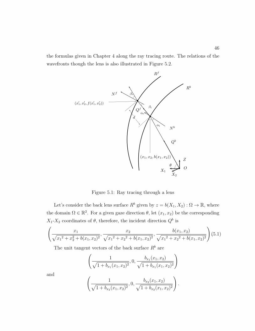
As shown in Figure 5.1, we will show the ray tracing process from eye center O
to the front lens surface Rf . All the perimeters will be evaluated according to
45
46
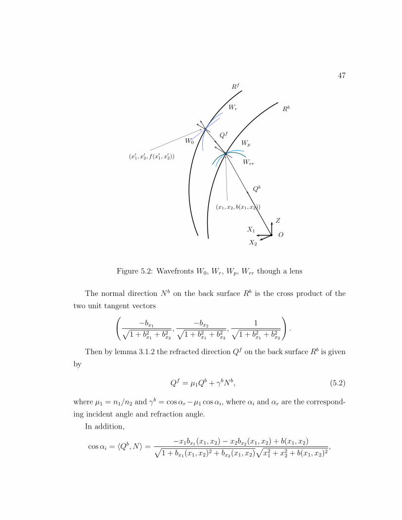
the formulas given in Chapter 4 along the ray tracing route. The relations of the
wavefronts though the lens is also illustrated in Figure 5.2.
Rf
Rb
O
(x1, x2, b(x1, x2))
(x′
1, x′
2, f(x′
1, x′
2))
Qb
N b
Nf
θ
Qf
b
b
b
d
βr
βi
αr
αi
X1
X2
Z
Figure 5.1: Ray tracing through a lens
Let’s consider the back lens surface Rb given by z = b(X1, X2) : Ω→ R, wherethe domain Ω ∈ R2. For a given gaze direction θ, let (x1, x2) be the corresponding
X1-X2 coordinates of θ, therefore, the incident direction Qb is(x1√
x12 + x22 + b(x1, x2)2,
x2√x12 + x22 + b(x1, x2)2
,b(x1, x2)√
x12 + x22 + b(x1, x2)2
).(5.1)
The unit tangent vectors of the back surface Rb are(1√
1 + bx1(x1, x2)2, 0,
bx1(x1, x2)√1 + bx1(x1, x2)
2
)and (
1√1 + bx2(x1, x2)
2, 0,
bx2(x1, x2)√1 + bx2(x1, x2)
2
).
47
Rf
Rb
O
b
b
b
(x′
1, x′
2, f(x′
1, x′
2))
W0
Wr
Wp
Wrr
Qb
Qf
(x1, x2, b(x1, x2))
X1
X2
Z
Figure 5.2: Wavefronts W0, Wr, Wp, Wrr though a lens
The normal direction N b on the back surface Rb is the cross product of the
two unit tangent vectors(−bx1√
1 + b2x1+ b2x2
,−bx2√
1 + b2x1+ b2x2
,1√
1 + b2x1+ b2x2
).
Then by lemma 3.1.2 the refracted direction Qf on the back surface Rb is given
by
Qf = µ1Qb + γbN b, (5.2)
where µ1 = n1/n2 and γb = cosαr−µ1 cosαi, where αi and αr are the correspond-
ing incident angle and refraction angle.
In addition,
cosαi = ⟨Qb, N⟩ = −x1bx1(x1, x2)− x2bx2(x1, x2) + b(x1, x2)√1 + bx1(x1, x2)
2 + bx2(x1, x2)√x21 + x22 + b(x1, x2)2
,
48
We have
cosαr =√
1− sin2 αr,
by Snell’s law, √1− sin2 αr =
√1− µ2
1 sin2 αi,
therefore
cosαr =√1− µ2
1(1− cos2 αi),
which also is
cosαr =√
1− µ21(1− < Qb, N⟩2).
Assume the refracted direction Qf intersects the front lens surface Rf at point
(x1′, x2
′, f(x1′, x2
′)) with travel distance d, then the normal direction of Rf at
coordinates (x1′, x2
′) is
(−fx1(x1′, x2
′),−fx2(x1′, x2
′), 1)√1 + fx1(x1
′, x2′)2 + fx2(x1′, x2′)2
.
Also, x1, x2, d, x′1, x
′2 should satisfy the equation
(x1, x2, b(x1, x2)) + d ·Qf = (x1′, x2
′, f(x1′, x2
′)). (5.3)
Assume the incident angle and the refracted angle on the front lens surface
are βi and βr, then
cos βi = ⟨Qf , N f⟩,
cos βr =√1− µ2
1(1− ⟨Qf , N f⟩2),
γf = cos βi − µ2 cos βr
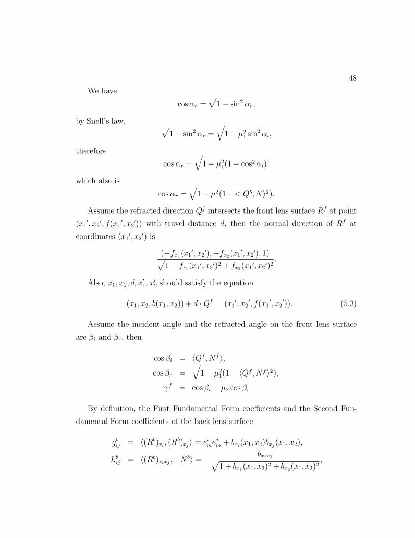
By definition, the First Fundamental Form coefficients and the Second Fun-
damental Form coefficients of the back lens surface
gbij = ⟨(Rb)xi, (Rb)xj
⟩ = eimejm + bxi
(x1, x2)bxj(x1, x2),
Lbij = ⟨(Rb)xixj
,−N b⟩ = −bxixj√
1 + bx1(x1, x2)2 + bx2(x1, x2)
2,
49
where
eij =
1 if i = j
0 otherwise
In particular, the mean curvature and the Gaussian curvature of Rb at point
(x1, x2) are given by
Hb =(1 + b2x1
)bx2x2 + (1 + b2x2)bx1x1 + 2bx1bx2bx1x2
2(√1 + b2x1
+ b2x2)3/2
,
Hb =bx1x1bx2x2 − b2x1x2
1 + b2x1+ b2x2
.
Similarly, the coefficients of the front lens surface are
gfij = ⟨(Rf )xi, (Rf )xj
⟩ = e1ie1j + e2ie2j + fxi(x′1, x
′2)fxj
(x′1, x′2),
Lfij = ⟨(Rf )xixj
, N f⟩ = −fxixj
(x1′, x2
′)√1 + fx1(x1, x2)
2 + fx2(x1, x2)2.
Consider the initial plane wavefront W0 on the refracted ray direction of the
front lens surface, the First Fundamental Form coefficients and Second Funda-
mental Form coefficients are:
gW011 = gW0
12 = 1, gW022 = 0,
LW011 = LW0
12 = LW022 = 0.
Then by theorem 4.4.3 and 4.4.4, the coefficients of the first refracted wavefront
are
gWrij = gfij − µ1ϕiϕj, (5.4)
LWrij = γfLf
ij, (5.5)
where
ϕ1 = −⟨(Rf )x1 , Qf⟩/µ2, ϕ2 = −⟨(Rf )x2 , Q
f⟩/µ2.
and
γf = −1/µ1 cos βr + cos βi.

50
By theorem 4.4.5, for the curvature of the first refracted wavefront, we have
HW0 = 0,
KW0 = 0,
∆W0 = 1,
∆f = 1 + fx1(x1′, x2
′)2 + fx2(x1′, x2
′)2,
ΘW0 = 1− (2− 2µ2)(ϕ2x1
+ ϕ2x2),
Θf = 1 + fx1(x1′, x2
′)2 + fx2(x1′, x2
′)2 − µ2(ϕ2x1gf11 + ϕ2
x2gf22 + 2ϕx1ϕx2g
f12),
ΠW = 0,
Πf = µ2ϕ2x1fx1x1(x1
′, x2′) + ϕ2
x2fx2x2(x1
′, x2′) + 2ϕx1ϕx2fx1x2(x1
′, x2′)√
1 + fx1(x1, x2)2 + fx2(x1, x2)
2,
σ = 0.
then,
HWr = γHR∆f
Θf− 1
2
Πf
Θf, (5.6)
KWr = γ2KR∆f
Θf. (5.7)
By theorem 4.3.3, we can get a simple representation of the curvatures of the
propagated wavefront before the back lens surface,
HWp =HWr − dKWr
1− 2dHWr + d2KWr, (5.8)
KWp =KWr
1− 2dHWr + d2KWr. (5.9)
To calculate the curvature of the refracted wavefront Wrr after the back lens
surface, we need the inverse matrix of the First Fundamental Form coefficients
g11 =gWr22
gWr11 g
Wr22 − (gWr
12 )2,
g12 = − gWr12
gWr11 g
Wr22 − (gWr
12 )2,
g22 =gWr11
gWr11 g
Wr22 − (gWr
12 )2.

51
and the derivative of the propagated wavefront under the coordinate system
(x1′, x2
′),
(Wp)xi′ = (Wr)xj
′ − d[gkjLWrji (Wr)xk
′ ]. (5.10)
The First Fundamental Form coefficients and the Second Fundamental Form co-
efficients of the propagated wavefront Wp are
gWp
ij = CikCjlgWrkl , (5.11)
and
LWp
ij = LWrij − dg
Wrkl L
Wrik L
Wrjl , (5.12)
where
Cij = eij − dgi1LWr1i − dgi2L
Wr2i ,
Now consider the refraction of the wavefront on the back lens surface. The
derivatives of the propagated wavefront under the coordinate system (x1, x2) are
(Wp)xi= (Rb)xi
− ηxiQf ,
where ηxi= −⟨(Rb)xi
, Qb⟩/µ1.
With the derivatives of the propagated wavefront Wp under the coordinate
system (x1, x2) by equation (5.10), the coordinate change matrix from (x1′, x2
′)
to (x1, x2) is
∂xi′
∂xj= gimbmj, (5.13)
where
bij = ⟨(Wp)xi, (Wp)xj
′⟩,
52
and giji,j=1,2 is the inverse matrix of the First Fundamental Form coefficient
matrix gWp
g11 =gWp
22
gWp
11 gWp
22 − (gWp
12 )2,
g12 = − gWp
12
gWp
11 gWp
22 − (gWp
12 )2,
g22 =gWp
11
gWp
11 gWp
22 − (gWp
12 )2.
The Second Fundamental Form coefficients of the propagated wavefront Wp
under the coordinate system (x1, x2) is
LWp
ij = LWpmn
∂xm′
∂xi
∂xn′
∂xj, (5.14)
Then by theorem 4.4.3 and 4.4.4, the coefficients of the second refracted wave-
front Wrr are
gWrrij = gbij − µ2
1ηiηj, (5.15)
LWrrij = µ1L
Wp
ij +(− γb
µ1
)Lb
ij. (5.16)
Therefore, the mean curvature and the Gaussian curvature of the second re-
fracted wavefront Wrr are
HWrr =1
2
LWrr11 gWrr
22 + LWrr22 gWrr
11 − 2LWrr12 gWrr
12
gWrr11 gWrr
22 − (gWrr12 )2
, (5.17)
KWrr =LWrr11 LWrr
22 − (LWrr12 )2
gWrr11 gWrr
22 − (gWrr12 )2
. (5.18)
5.2 Front surface design
While we can manipulate both the front lens surface Rf and the back lens surface
Rb to reach the minimum functional value, in practical design, we can either fix
the back lens surface Rb as a sphere or a toroidal surface to have a front surface

53
design, or we can make a back lens surface design by fixing the front lens surface
Rf .
If we fix the back lens surface as a sphere or a toroid, the design objective
functional is
J (Rf ) =
∫Ω
β(HWrr(θ)− P (θ))2dθ + α
∫Ω
(AWrr)2(θ)dθ,
where HWrr and KWrr are calculated through formulas (5.4), (5.5), (5.11), (5.12),
(5.13), ( 5.14), ( 5.15), ( 5.16), (5.17) and (5.18).
5.2.1 Gradient of the design objective functional
To calculate the gradient of the design objective functional with respect to the
front lens surface, We add a perturbation δf on the front lens surface f , By
equation 5.3,
b(x1, x2) + (d+ δd)Qbz = (f + δf)(x1 + (d+ δd)Qb
x1, x2 + (d+ δd)Qb
x2),
Taylor expansion gives
b(x1, x2) + dQbz + δdQb
z = f(x1 + dQbx1, x2 + dQb
x2)
+fx1(x1 + dQbx1, x2 + dQb
x2)δdQb
x1
+fx2(x1 + dQbx1, x2 + dQb
x2)δdQb
x2
+δf(x1 + dQbx1, x2 + dQb
x2),
therefore,
δd =δf
Qbz − fx1(x1
′, x2′)Qbx1
+ fx2(x1′, x2′)Qb
x2
, (5.19)
then,
δx1′ = δdQb
x1,
δx2′ = δdQb
x2.

54
Similarly, we can have the perturbation of the coefficients of the front lens
surface with respect to δf ,
δgfij = 2fxi(x1
′, x2′)fxixm(x1
′, x2′)δxm
′ + fxj(x1
′, x2′)fxjxm(x1
′, x2′)δxm
′,
and
δLfij =
δfxixj(x1
′, x2′) + fxixjxm(x1
′, x2′)δxm
′√1 + f 2
x1(x1′, x2′) + f 2
x2(x1′, x2′)
+fxixj
(x1′, x2
′)
(1 + f 2x1(x1′, x2′) + f2
x2(x1′, x2′))3/2
(2fxm(x1′, x2
′)δfxm(x1′, x2
′)
+fxmxn(x1′, x2
′)δxn′).
Then the perturbation of mean curvature and Gaussian curvature of the front
lens surface are
δHf =1
2
δgf11Lf22 + gf11δL
f22 + δgf22L
f11 + gf22δL
f11 − 2δgf12L
f12 − 2gf12δL
f12
gf11gf22 − (gf12)
2
+gf11L
f22 + gf22L
f11 − 2gf12L
f12
(gf11gf22 − (gf12)
2)2(δgf11g
f22 + gf11δg
f22 − (2gf12δg
f12)), (5.20)
δKf =δLf
11Lf22 + Lf
11δLf22 − 2Lf
12δLf12
gf11gf22 − (gf12)
2
+Lf11L
f22 − (Lf
12)2
(gf11gf22 − (gf12)
2)2(δgf11g
f22 + gf11δg
f22 − 2gf12δg
f12) (5.21)
According to equations (5.4) and (5.5), the perturbation of the First Funda-
mental Form coefficients and the Second Fundamental Form coefficients of the
first refracted wavefront Wr are
δgWrij = δgfij − µ2
1(ϕiδϕj + ϕjδϕi)
δLWrij = δγfLf
ij + γfδLfij,
55
where
δϕi = −⟨δ(Rf )iQf⟩/µ2,
δγf = −1/µ1δ cos βr − δ cos βi,
δ cos βi = ⟨Qf , δN f⟩,
δ cos βr =1
2
√1− µ1(1− ⟨Qf , N f⟩)(1− µ1(1− 2⟨Qf , N f⟩⟨Qf , δN f⟩)).
Therefore, the perturbation of mean curvature and Gaussian curvature of the
first refracted wavefront are
δHWr = δγfHf ∆f
Θf+ γfδHf ∆
f
Θf+ γHR δ∆
fΘf +∆fδΘf
(Θf )2
−1
2
δΠfΘf − ΠfδΘf
(Θf )2,(5.22)
δKWr = 2γfδγfKf ∆f
Θf+ γ2δKf ∆
f
Θf+ γ2Kf δ∆
fΘf −∆fδΘf
(Θf )2. (5.23)
where
δ∆f = 2fx1(x1′, x2
′)(fx1x1(x1′, x2
′)δx1′ + fx1x2(x1
′, x2′)δx2
′ + δfx1(x1′, x2
′))
2fx2(x1′, x2
′)(fx1x1(x1′, x2
′)δx1′ + fx1x2(x1
′, x2′)δx2
′ + δfx2(x1′, x2
′)),
δΘf = δ∆f − µ2(2ϕx1δϕx1gf11 + ϕ2
x1δgf11 + 2ϕx2δϕx2g
f22 + ϕ2
x2δgf22 + 2δϕx1ϕx2g
f12
+2ϕx1δϕx2gf12 + 2ϕx1ϕx2δg
f12),
δΠf = µ21
(δϕiϕjfxixj
(x1′, x2
′) + ϕiδϕjfxixj(x1
′, x2′)√
1 + fx1(x1, x2)2 + fx2(x1, x2)
2
+ϕiϕj(δfxixj
(x1′, x2
′) + fxixjxm(x1′, x2
′)δx′m)√1 + fx1(x1, x2)
2 + fx2(x1, x2)2
−1
2
ϕiϕjfxixj(x1
′, x2′)
(1 + fx1(x1, x2)2 + fx2(x1, x2)
2)32
δ∆f
).
By (5.11),
δgWp
ij = CjlgWrkl δCik + Cikg
Wrkl δCjl + CikCjlδg
Wrkl , ,
56
where
δCij = −dgi1δLWr1i − dL
Wr1i δg
i1 − gi1LWr1i δd
−dgi2δLWr2i − dL
Wr2i δg
i2 − gi2LWr2i δd,
and by (5.12),
δLWp
ij = δLWrij − dg
Wrkl L
Wrik δL
Wrjl − dg
Wrkl L
Wrjl δL
Wrik
−dLWrik L
Wrjl δg
Wrkl − g
Wrkl L
Wrik L
Wrjl δd, ,
By (5.14),
δLWp
ij =∂xm
′
∂xi
∂xn′
∂xjδLWp
mn + LWpmn
∂xm′
∂xiδ∂xn
′
∂xj+ LWp
mn
∂xn′
∂xjδ∂xm
′
∂xi.
The perturbation on the front lens should not be related to the back lens
surface, so the perturbation of the First Fundamental Form coefficients and the
Second Fundamental Form coefficients of the back lens surface should all be 0,
which are
δgbij = 0,
δLbij = 0.
Then by (5.15), the perturbation of the First Fundamental Form coefficients
are
δgWrrij = 0.
and by the Second Fundamental Form coefficients are
δLWrrij = µ1δL
Wp
ij .
Then the perturbation of the mean Curvature and the Gaussian Curvature of
the second refracted wavefront Wrr are
δHWrr =1
2
gWrr22 δLWrr
11 + gWrr11 δLWrr
22 − 2gWrr12 δLWrr
12
gWrr11 gWrr
22 − (gWrr12 )2
,
δKWrr =LWrr
22 δLWrr11 + LWrr
11 δLWrr22 − 2LWrr
12 δLWrr12
gWrr11 gWrr
22 − (gWrr12 )2
.

57
5.2.2 Optimization on the wavefront before the back lens
surface
From subsection 5.1, we may use formulas (5.6), (5.7), (5.8) and (5.9) to calculate
the mean curvature and the Gaussian curvature of the wavefront before the back
lens surface. We can see that the representation is much simpler than the wave-
front after the back lens surface, which is using (5.4), (5.5), (5.11), (5.12), (5.13),
(5.14), (5.15), (5.16), (5.17) and (5.18).
If we change the design objective functional to be optimizing on the wavefront
before the back lens surface,
J (Rf ) =
∫Ω
β(HWp(θ)− P (θ))2dθ +∫Ω
α(AWp)2(θ)dθ,
where P is the approximated power before the back lens surface. We need to find
the approximated power before the back lens surface based on the desired power
of the wavefront after the back lens surface. The front lens surface obtained by
optimizing on this approximated power should be efficient.
Assume the desired power of the lens is P , we want to find the desired power
of the wavefront before the back lens surface P . Since the perfect shape of the
refracted wavefront should be, at each point (x1, x2), a sphere with power P (x1, x2)
and the astigmatism 0. Assume the principle curvature of the desired wavefront
at point (x1, x2) is κ1 and κ2, then
κ1 + κ22
= P (x1, x2),
κ1 − κ2 = 0,
which means κ1 = κ2 = P (x1, x2).
Since the principal curvature κ1 and κ2 are the roots of equations
det
([LWrr11 LWrr
12
LWrr21 LWrr
22
]− κ
[gWrr11 gWrr
12
gWrr21 gWrr
22
])= 0,

58
κ1 and κ2 satisfies
(LWrr11 LWrr − (LWrr
12 )2)− κ1(LWrr11 gWrr
22 + LWrr11 gWrr
22 − 2LWrr12 gWrr
12 )
+κ21(gWrr11 gWrr
22 − (LWrr12 )2) = 0
(LWrr11 LWrr − (LWrr
12 )2)− κ2(LWrr11 gWrr
22 + LWrr11 gWrr
22 − 2LWrr12 gWrr
12 )
+κ22(gWrr11 gWrr
22 − (LWrr12 )2) = 0
Since at every point the wavefront is a spherical shape, we can make the as-
sumption that the coordinate system (X1, X2) is the principal coordinate system.
Under the principal coordinate system (X1, X2), LWrr12 and gWrr
12 are equal to 0.
Then we have
LWrr11 = κ1g
Wrr11 , LWrr
22 = κ2gWrr22 .
By theorem 4.4.4, we have the desired Second Fundamental Form of the wave-
front before the back lens surface Rb under coordinate system x1, y
LWp
ij = µ1LWrrij + γ1L
bij.
By theorem 4.4.3, the desired First Fundamental Form of the wavefront before
the back lens surface Rb under coordinate system x1, y is
gWp
ij = gbij − ϕiϕj.
Therefore the desired power of the wavefront before the back lens surface can
be calculated by the formula
P =L
Wp
11 gWp
22 + LWp
22 gWp
11 − 2LWp
12 gWp
12
gWp
11 gWp
22 − (gWp
11 )2,
then by (5.11) and (5.12),
P =(µ1κ1g
Wrr11 + γ1L
bij)g
Wp
22 + LWp
22 gWp
11 − 2LWp
12 gWp
12
gWp
11 gWp
22 − (gWp
11 )2(5.24)

59
The representation of the gradient of the mean curvature and the Gaussian
curvature of Wp are much simpler than the mean curvature and Gaussian curva-
ture of Wrr,
δHWp =[δHWr − (KWrδd+ dδKWr)](1− 2dHWr + d2KWr)
(1− 2dHWr + d2KWr)2
−(HWr − dKWr)[−2(dδHWr +HWrδd) + (2dKWrδd+ d2δKWr)]
(1− 2dHWr + d2KWr)2,
δKWp =δKWr(1− 2dHWr + d2KWr)
(1− 2dHWr + d2KWr)2
−KWr [−2(dδHWr +HWrδd) + (2dKWrδd+ d2δKWr)]
(1− 2dHWr + d2KWr)2,
where δHWr , δKWr and δd can be calculated by (5.22), (5.23), and (5.19).
5.3 Back surface design
As we fix the front lens surface as a sphere or a toroid, the design objective
functional is
J (Rb) =
∫Ω
β(HWrr(θ)− P (θ))2dθ +∫Ω
α(AWrr)2(θ)dθ.
Consider a fixed gaze direction θ = (φ, ψ), a different back lens surface may
give a different intersection point, hence it should be reasonable to use (φ, ψ) as
the coordinate rather than (x, y) coordinates of the intersect point. If we assume
the distance from the eye center O to the back lens surface Rb is ρ(φ, ψ), then
Rb = (ρ(φ, ψ) cosφ cosψ, ρ(φ, ψ) cosφ sinψ, ρ(φ, ψ) sinφ).
Then the mean curvature and Gaussian curvature of the second refracted wave-
front Wrr can be calculated by (5.4), (5.5), (5.11), (5.12), (5.15) and (5.16).

60
5.4 Use of travel distance to represent lens sur-
face
In previous sections, we show a way to calculate the curvature with direct surface
representation, this evaluation requires to compute a line-surface intersection for
every gaze direction, which has to be done numerically and time-consuming. While
in [11], J. Loost. shows a representation of the surface by the travel distance. In
this way, we can calculate the intersection directly.
Consider the sample point (x1, x2, b(x1, x2)) on the back lens surface, we can
parameterize the front surface Rf by the travel distance ϕ(x1, x2) from the back
lens surface Rb and the front lens surface Rf under coordinate system (X1, X2) of
Rb,
Rf (x1, x2) = Rb(x1, x2) + ϕ(x1, x2)Qf (x1, x2).
5.5 Lens surface representation by splines
5.5.1 An abstracted linear interpolation scheme
Most of the linear approximation schemes (such as interpolation, least squares
approximation) fit into the following abstract framework, for a given function g ,
we attempt to construct an approximation Pg =∑n
j=1 αjfj with fjnj=1 certain
fixed functions, on the domain Ω on which g is defined. We construct the specific
approximation by interpolation with respect to linear functionals λini=1, i.e. by
the requirement that
λi(Pg) = λi(g), i = 1, . . . , n,
for certain fixed linear interpolation conditions or linear functional λ1, . . . , λn.
We might choose
λi(g) = g(ti), i = 1, . . . , n

61
for some t1⟨· · · < tn, this is ordinary interpolation, which is used in our numerical
scheme.
Definition 5.5.1. Assume the linear span
F = span (fj)nj=1 :=
n∑j=1
αjfj : α ∈ Rn
of the fj’s and linear span
Λ = span (λi)ni=1 :=
n∑i=1
αiλi : α ∈ Rn,
We can define linear interpolation problem (LIP) as follows: Find an f ∈ F for a
given g so that
λ(f) = λ(g), for all λ ∈ Λ.
We say that the LIP given by F and Λ is correct if it has exactly one solution
for every g ∈ U. Here, U is some linear space of functions, all defined on the same
domain of g, and U ⊇ F. In our numerical scheme, Ck×k(X × Y ) is a space of all
k-th continuous functions on X = [a, b]× [c, d].
Definition 5.5.2. [5] Let U be a linear space of functions, all defined on some
set X into R, and V be, similarly, a linear space of functions defined on some set
Y into R. For each u ∈ U and v ∈ V, the rule
w(x, y) := u(x)v(y) all (x, y) ∈ X × Y,
defines a function on X × Y called the tensor product of u with v and denoted by
u⊗ v.
The set of all finite linear combination of functions on X×Y of the form u⊗vfor some u ∈ U and some v ∈ V is called the tensor product of U with V and is
denoted by u⊗ v. Thus,
U⊗ V := n∑
i=1
n∑j=1
αij(ui ⊗ vj) : αij ∈ R, ui ∈ U, vj ∈ V, i = 1, . . . , n,
and U⊗ V is a linear space of functions on X × Y .
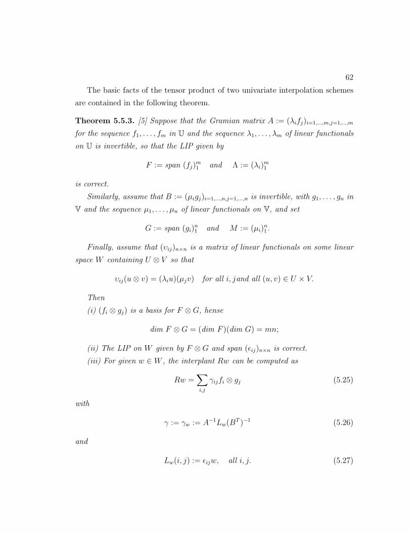
62
The basic facts of the tensor product of two univariate interpolation schemes
are contained in the following theorem.
Theorem 5.5.3. [5] Suppose that the Gramian matrix A := (λifj)i=1,...,m,j=1,...,m
for the sequence f1, . . . , fm in U and the sequence λ1, . . . , λm of linear functionals
on U is invertible, so that the LIP given by
F := span (fj)m1 and Λ := (λi)
m1
is correct.
Similarly, assume that B := (µigj)i=1,...,n,j=1,...,n is invertible, with g1, . . . , gn in
V and the sequence µ1, . . . , µn of linear functionals on V, and set
G := span (gi)n1 and M := (µi)
n1 .
Finally, assume that (υij)n×n is a matrix of linear functionals on some linear
space W containing U ⊗ V so that
υij(u⊗ v) = (λiu)(µjv) for all i, jand all (u, v) ∈ U × V.
Then
(i) (fi ⊗ gj) is a basis for F ⊗G, hense
dim F ⊗G = (dim F )(dim G) = mn;
(ii) The LIP on W given by F ⊗G and span (ϵij)n×n is correct.
(iii) For given w ∈ W , the interplant Rw can be computed as
Rw =∑i,j
γijfi ⊗ gj (5.25)
with
γ := γw := A−1Lw(BT )−1 (5.26)
and
Lw(i, j) := ϵijw, all i, j. (5.27)

63
5.5.2 Tensor-product B-spline function
Tensor-product B-Spline function is employed to represent the lens surface. Al-
though applicability of tensor product method is limited, but when their use can
be justified, then these method should be used since they are extremely efficient
compared to other surface approximation techniques.
First, let’s introduce the univariate B-spline function.
Definition 5.5.4. [5] Given m real value ti called knots, with
t0 ≤ t1 ≤ · · · ≤ tm.
A B-spline of degree n is a parametric curve
S : [t0, tm] 7→ R
composed of a linear combination of basis B-spline function Bni of degree n,
S(t) =m−n−2∑
i=1
aiBni (t), t ∈ [tn, tn−m−1]
The m-n-1 basis B-splines of degree n can be defined, for n = 0, 1, . . . ,m− 2,
using the Cox-de Boor recursion formula. ([5])
B0j =
1, if tj ≤ t ≤ tj+1
0, otherwisej = 1, . . . ,m− 2
and
Bnj (t) =
t− tjtj+n − tj
Bn−1j (t) +
tj+n+1 − ttj+n+1 − tj+1
Bn−1j+1 (t), j = 0, . . . ,m− n− 2
In particular, suppose t = timi=1 are the uniform knots, the non-recursive
definition of the m− n− 1 basis B-splines for a given value n is
Bnj (t) =
n+ 1
n
n+1∑i=0
ωi,n(t− tj − ti)n+,

64
with
ωi,n =n+1∏
j=0,j =i
1
tj − ti,
where
(t− ti)n+ =
(t− ti − tj)n, if t ≥ ti + tj
0, otherwise
We may denote the linear space of B-splines of order n with knot sequence t
as
Bn,t = span (Bnj )
n1 .
Without loss of generality, suppose Ω is the unit square domain
Ω = [0, 1]⊗ [0, 1].
The uniform partition is the partition of Ω by the following knot lines
mx− i = 0, ny − j = 0,
where m and n are the numbers of the rectangles in the x and y direction respec-
tively and i = 1 . . .m, j = 1 . . . n.
Now we consider the following situation in Theorem 5.5.3 of tensor product
B-spline functions.
Suppose we have
F = Bh,s,with s = (si)m+h1 , and λi = σi, i = 1, . . . ,m
with σ1 < · · · < σm.
This problem is correct if and only if si < σi < si+h for all i based on this
following theorem
Theorem 5.5.5. [4] (Schoenberg-Whitney Theorem) The matrix (Bj(τi))i=1,...,n,j=1,...,n
of linear systemn∑
j=1
αjBj(τi) = g(τi), i = 1, . . . , n.
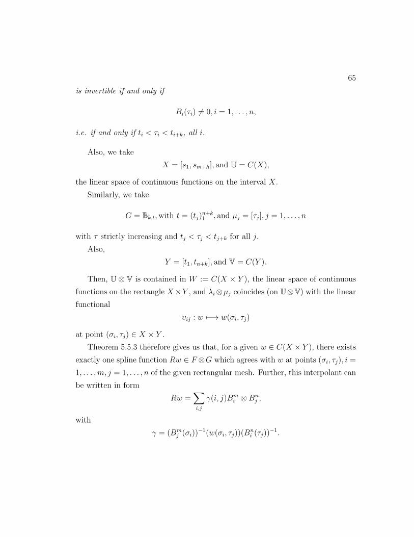
65
is invertible if and only if
Bi(τi) = 0, i = 1, . . . , n,
i.e. if and only if ti < τi < ti+k, all i.
Also, we take
X = [s1, sm+h], and U = C(X),
the linear space of continuous functions on the interval X.
Similarly, we take
G = Bk,t,with t = (tj)n+k1 , and µj = [τj], j = 1, . . . , n
with τ strictly increasing and tj < τj < tj+k for all j.
Also,
Y = [t1, tn+k], and V = C(Y ).
Then, U ⊗ V is contained in W := C(X × Y ), the linear space of continuous
functions on the rectangle X×Y , and λi⊗µj coincides (on U⊗V) with the linear
functional
υij : w 7−→ w(σi, τj)
at point (σi, τj) ∈ X × Y .
Theorem 5.5.3 therefore gives us that, for a given w ∈ C(X × Y ), there exists
exactly one spline function Rw ∈ F ⊗G which agrees with w at points (σi, τj), i =
1, . . . ,m, j = 1, . . . , n of the given rectangular mesh. Further, this interpolant can
be written in form
Rw =∑i,j
γ(i, j)Bmi ⊗Bn
j ,
with
γ = (Bmj (σi))
−1(w(σi, τj))(Bni (τj))
−1.
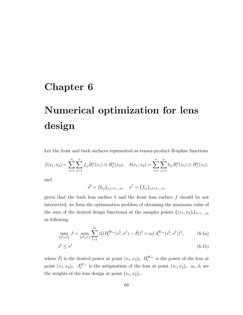
Chapter 6
Numerical optimization for lens
design
Let the front and back surfaces represented as tensor-product B-spline functions
f(x1, x2) =n∑
i=1
n∑j=1
fijBni (x1)⊗Bn
j (x2), b(x1, x2) =n∑
i=1
n∑j=1
bijBni (x1)⊗Bn
j (x2),
and
sb = biji,j=1,...,n, sf = fiji,j=1,...,n,
given that the back lens surface b and the front lens surface f should be not
intersected, we form the optimization problem of obtaining the minimum value of
the sum of the desired design functional at the samples points (x1, x2)ll=1,...,m
as following
minsb,sf
J = minsb,sf
m∑l=1
βl(HWrrl (sb, sf )− Pl)
2 + αl(AWrrl (sb, sf ))2, (6.1a)
sb ≤ sf (6.1b)
where Pl is the desired power at point (x1, x2)l. HWrrl is the power of the lens at
point (x1, x2)l. AWrrl is the astigmatism of the lens at point (x1, x2)l. αl, βl are
the weights of the lens design at point (x1, x2)l.
66

67
In a front lens surface design, we usually fix the back lens surface as a spherical
surface or a toric surface, then want to find (sf )∗ = f∗iji,j=1,...,n such that
J((sf )∗) = minsf
m∑l=1
βl(HWrrl (sf )− Pl)
2 + αl(AWrrl (sf ))2, (6.2a)
sb ≤ sf . (6.2b)
In a back lens surface design, we fix the front lens surface as the spherical
surface and the toric surface, then try to solve for a minimum design objective
functional J(sb) in constrained optimization problem
minsb
m∑l=1
βl(HWrrl (sb)− Pl)
2 + αl(AWrrl (sb))2, (6.3a)
sb ≤ sf . (6.3b)
We will focus on the front lens surface design problem (6.2) in the following
sections, let
u2 = sf − sb,where u = uiji,j=1,...,n, (6.4)
then rearranging the equation gives
sf = sb + u2 ≥ sb. (6.5)
Therefore, substituting (6.4) into optimization problem (6.2), the constrain
(6.2b) is satisfied, then we have an unconstrained optimization problem
minuJ(u) = min
u
m∑l=1
βl(HWrrl (u2 + sb)− Pl)
2 + αl(AWrrl (u2 + sb))2, (6.6)
where u ∈ Rn×n.
We need to find a minimizer for this nonlinear unconstrained optimization
problem (6.6). Assume J is a twice continuously differentiable, we may be able
to tell that a point u∗ is a local minimizer by examining just the gradient ∇J(u∗)and the Hessian ∇2J(u∗).

68
In the following sections, we will give some introduction of the unconstrained
optimization theory. Gradient, Hessian and the approximated Hessian of the
objective design functional will be discussed and numerical optimization methods
such as Gradient method, Newton’s method and Quasi Newton’s method will be
employed on obtaining the minimizer of the optimization problem.
6.1 Unconstrained Optimization
Definition 6.1.1. [13]
1. A point u∗ is a global minimizer of J if J(u∗) < J(u) for all u.
2. A point u∗ is a local minimizer of J if there is a neighborhood N of u∗ such
that J(u∗) ≤ J(u) for u ∈ N .
3. A point u∗ is a strict local minimizer of J if there is a neighborhood N of
u∗ such that J(u∗) < J(u) for all u ∈ N with u = u∗.
Taylor’s theorem is the key tool to our analysis of the unconstrained optimiza-
tion problem.
Theorem 6.1.2. Suppose J : Rn → R is continuously differentiable and that
p ∈ Rn. Then we have that
J(u+ p) = J(u) +∇J(u+ tp)Tp.
for some t ∈ (0, 1). Moreover, if J is twice continuously differentiable, we have
that
∇J(u+ p) = ∇J(u) +∫ 1
0
∇2J(u+ tp)pdt.
and that
J(u+ p) = J(u) +∇J(u)Tp+ 1
2pTJ(u+ tp)p,
for some t ∈ (0, 1).

69
By Taylor’s theorem, if x∗ is a local minimizer and f is continuously differen-
tiable in an open neighborhood of x∗, then ∇f(x∗) = 0. This condition is called
First-Order Necessary Conditions. By adding one more condition that ∇2f is
continuous in an open neighborhood of x∗ to First-Order Necessary Conditions,
we have the Second-Order Necessary Conditions: ∇f(x∗) = 0 and ∇2f(x∗) is
positive definite.
Theorem 6.1.3. ([6]) Suppose that ∇2f(x∗) is continuous in an open neighbor-
hood of x∗ and that ∇f(x∗) = 0 and ∇2f(x∗) is positive definite . Then x∗ is a
strict local minimizer of f .
6.2 Gradients
The gradient ∇J(u∗) of the design objective functional J then is
∇J(sb, sf ) =m∑l=1
2βl(HWrrl (sb, sf )− Pl)∇HWrr
l (sb, sf ) + 2αl(AWrrl (sb, sf ))∇(AWrr
l (sb, sf )),
∇HWrr(sb, sf ) and ∇AWrr(sb, sf ) can be calculated according to Section 5.2.1
depending on the front surface lens design or the back surface lens design.
6.3 Approximated Hessian
Calculating the Hessian ∇2J directly would be time consuming and unstable,
so we use BFGS method to give an approximation of the inverse matrix of the
Hessian on every iteration of our optimization process (see [13]).
The derivation of the approximated Hessian matrix starts from approximating
the design objective functional J(u) at the current iterate uk:
mk(p) = Jk +∇JTk p+
1
2pTDkJp.
Here Dk is an n × n symmetric positive definite matrix that will be updated at
every iteration.

70
The minimizer uk of this convex quadratic model is
pk = −(Dk)−1∇J,
which can be used as the search direction, and the new search iterate is
uk+1 = uk + pk.
Dk is the approximated Hessian.
In order to calculate the approximated Hessian, suppose we have a new iterate
xk+1, then the new quadratic model is
mk+1(p) = Jk+1 +∇JTk+1p+
1
2pTDk+1Jp.
One requirement for Dk+1 is that the gradient of mk+1 should match the gra-
dient of the desired design functional J at the latest two iterates xk and xk+1.
Therefore, we have
∇mk+1(0) = ∇Jk+1,
∇mk+1(−pk) = ∇Jk+1 −Dk+1pk = ∇Jk.
By rearranging, we obtain
Dk+1pk = ∇Jk+1 −∇Jk, (6.7)
To simplify the notation, we define the vectors,
sk = xk+1 − xk, yk = ∇Jk+1 −∇Jk,
so that (6.7) becomes
Dk+1sk = yk. (6.8)
The equation is referred to as the secant equations.
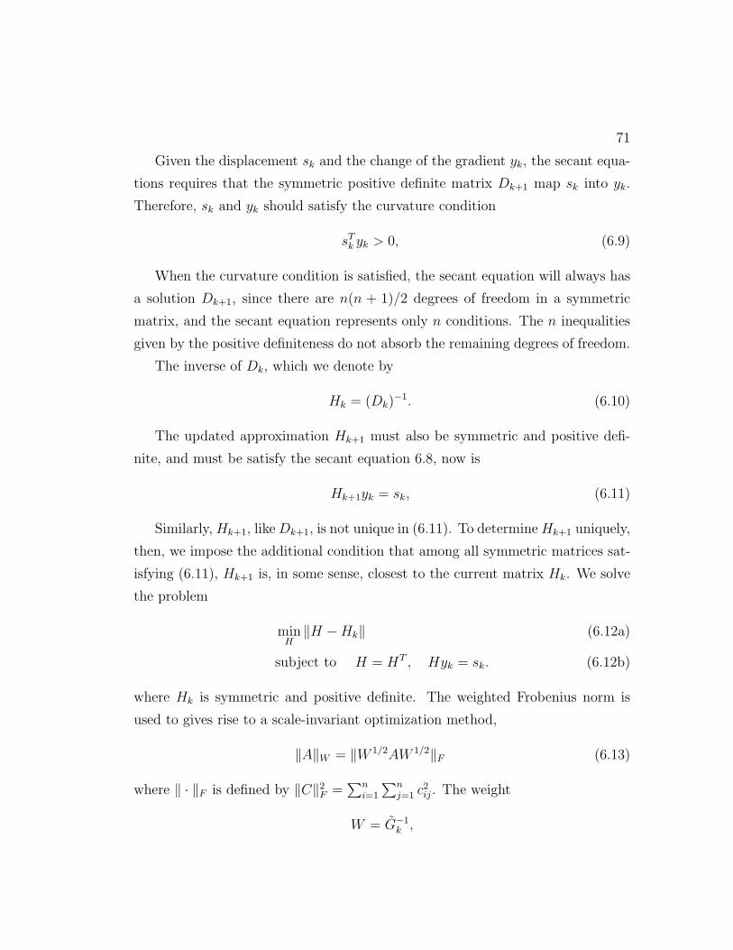
71
Given the displacement sk and the change of the gradient yk, the secant equa-
tions requires that the symmetric positive definite matrix Dk+1 map sk into yk.
Therefore, sk and yk should satisfy the curvature condition
sTk yk > 0, (6.9)
When the curvature condition is satisfied, the secant equation will always has
a solution Dk+1, since there are n(n + 1)/2 degrees of freedom in a symmetric
matrix, and the secant equation represents only n conditions. The n inequalities
given by the positive definiteness do not absorb the remaining degrees of freedom.
The inverse of Dk, which we denote by
Hk = (Dk)−1. (6.10)
The updated approximation Hk+1 must also be symmetric and positive defi-
nite, and must be satisfy the secant equation 6.8, now is
Hk+1yk = sk, (6.11)
Similarly, Hk+1, likeDk+1, is not unique in (6.11). To determineHk+1 uniquely,
then, we impose the additional condition that among all symmetric matrices sat-
isfying (6.11), Hk+1 is, in some sense, closest to the current matrix Hk. We solve
the problem
minH∥H −Hk∥ (6.12a)
subject to H = HT , Hyk = sk. (6.12b)
where Hk is symmetric and positive definite. The weighted Frobenius norm is
used to gives rise to a scale-invariant optimization method,
∥A∥W = ∥W 1/2AW 1/2∥F (6.13)
where ∥ · ∥F is defined by ∥C∥2F =∑n
i=1
∑nj=1 c
2ij. The weight
W = G−1k ,

72
where Gk is the average Hessian defined by
Gk =
[∫ 1
0
∇2J(xk + τpk)dτ
]. The unique solution Hk+1 to 6.12 is given by
(BFGS) Hk+1 = (1− ρkskyTk )Hk(1− ρkskyTk ) + ρksksTk , (6.14)
where
ρk =1
yTk sk.
The update formula for the approximate Hessian Dk can be obtained by ap-
plying Sherman-Morrison-Woodbury formula [16] to 6.14.
Lemma 6.3.1. Assume A is a square nonsingular matrix. Let U and V be ma-
trices in Rn×p. If
A = A+ UV T ,
then
A−1 = A−1 − A−1U(I + V TA−1U)−1V TA−1. (6.15)
Proof. Consider the following block matrix[A U
V −I
][X
Y
]=
[I
0
].
Expanding of the above equation gives
AX + UY = I, (6.16a)
V X − Y = 0, (6.16b)
which is equivalent to
(A+ UV )X = I.
Therefore,
X = (A+ UV )−1 = (A)−1.
73
Eliminating (6.16a) gives
X = A−1(I − UY ). (6.17)
Substituting (6.17) to (6.16b), we obtain
Y = (I + V A−1U)−1V A−1. (6.18)
Then 6.16a can be transformed into
AX + U(I + V A−1U)−1V A−1 = I,
therefore,
(A)−1 = X−1 = A−1 − A−1U(I + V TA−1U)−1V TA−1.
The approximated Hessian by BFGS method is therefore
(BFGS) Bk+1 = Bk −Bksks
TkBk
sTkBksk+yky
Tk
yTk sk. (6.19)
6.4 Outline of a computational algorithm
A computational algorithm is stated as in 6.4,
6.5 Method of optimization
In unconstrained optimization, we minimize an objective function that depends
on real variables, with no restriction on the values of these variables. The math-
ematical formulation is
minuJ(u), (6.20)
where x ∈ Rn and f : Rn → R is a smooth function.
74
Set the initial front lens surface u0 as a spherical surface or a toric surface which
is close to the back surface, convergence tolerance ϵ > 0;
k ← 0;
while ∥∇J∥ ≤ ϵ; do
Obtain the minimizer search step pk by Gradient method, Newton’s method
or Quasi-Newton’s method;
Set xk+1 = xk + pk;
k ← k + 1;
end while
All algorithms for unconstrained optimization require to start with a starting
point x0, which should be a reasonable estimate of the solution. Beginning at x0,
optimization algorithm generates a sequence of iterates xk∞k=1 that terminates
when ∥∇J∥ is small enough. In order to decide how to move from xk to a new
iterate xk+1, the algorithm use information of J at xk to find a new iterate xk+1
with a lower function value J(xk+1) than J(xk).
6.5.1 Gradient method
From the k-th iterate xk, for any unit search direction d and the step size parameter
α, by Taylor Theorem (6.1.2), we have
J(xk + αd) = J(xk) + αdT∇J(xk) +1
2α2dT∇2J(xk + td)d, for some t ∈ (0, α).(6.21)
The rate of change in f along d at xk is the coefficient of α, dT∇J(xk). Hence,to get the most rapid decrease search direction d, we want to solve the problem
minddT∇J(xk), subject to ∥d∥ = 1. (6.22)
Since
dT∇J(xk) = ∥d∥∥∇J(xk)∥ cos θ,
where θ is the angle between d and ∇J(xk), also with
∥d∥ = 1,
75
we have
dT∇J(xk) = ∥∇J(xk)∥ cos θ.
The objective function in 6.22 is minimized when θ = π, in other words, the
solution to 6.22 is
p = −∇J(xk)/∥∇J(xk)∥,
as claimed.
The steepest descent method is a line search method that moves along dk =
−∇J(xk) at every k-th step. The step size αk should be chosen by a variety ways.
Wolfe conditions is a efficient requirement on performing an inexact line search.
Lemma 6.5.1. (Wolfe condition)
J(xk + αkdk) ≤ J(xk) + c1αk∇JT (xk)dk, (6.23a)
|∇J(xk + αkdk)Tdk| ≤ c2|∇J(xk)Tdk|, (6.23b)
with 0 < c1 < c2 < 1.
6.5.2 Newton’s method
Newton’s method is derived from the second-order Taylor series approximation to
J(xk + d), which is
J(xk + p) ≈ J(xk) + pT∇J(xk) +1
2pT∇2J(xk)p , mk(p). (6.24)
Notice that the derivative of mk(p) should be eliminated on pk that minimizes
mk(p), we obtain
∇pmk(pk) = 0,
which is
∇2J(xk)pk = −∇J(xk).
Assume that ∇2J(xk) is positive definite, then
pk = −(∇2J(xk))−1∇J(xk). (6.25)

76
Newton’s method can achieve a quadratic convergence rate. However, the
main drawback is the need for the Hessian ∇2J(xk). Explicit computation of the
second derivatives is a time-consuming process.
6.5.3 Quasi-Newton method
Quasi-Newton method is an alternative method of Newton’s method in that they
don’t require computation of the Hessian and attain the superlinear rate of con-
vergence.
In place of the true Hessian∇2J(xk), they use an BFGS Hessian approximation
Bk, which is updated after each step. The calculation of the approximated Hessian
Bk and the inverse of the approximated Hessian Hk is stated in the section 6.3.
The formulas are
(BFGS) Bk = Bk−1 −Bk−1sk−1s
Tk−1Bk−1
sTk−1Bk−1sk−1
+yk−1y
Tk−1
yTk−1sk−1
, (6.26)
(BFGS) Hk−1 = (1− ρk−1sk−1yTk−1)Hk−1(1− ρk−1sk−1y
Tk−1)
+ρk−1sk−1sTk−1, (6.27)
where sk−1 = xk − xk−1, yk−1 = ∇Jk −∇Jk−1, and ρk−1 =1
yTk−1sk−1
The basic algorithm of Quasi-Newton method using BFGS approximation is
6.5.3

77
Algorithm 1 BFGS Quasi-Newton Method
Set the initial front lens surface u0 as a spherical surface or a toric surface
which is close to the back surface, convergence tolerance ϵ > 0, inverse Hessian
approximation H0;
k ← 0;
while ∥∇J∥ ≤ ϵ; do
Compute the search direction
dk = −Hk∇J(xk); (6.28)
Set xk+1 = xk + αkdk where αk is computed from a line search procedure
satisfy the Wolfe conditions 6.5.1;
Define sk = xk+1 − xk and yk = ∇Jk+1 −∇Kk;
Compute Hk+1 by the formula of 6.14;
k ← k + 1;
end while
Chapter 7
Numerical Result
In practise, lenses are designed on a circular region of diameter 80mm with grid
size of 2mm or 4mm. In our numerical example, we choose the design region
to be a square domain [−22, 22] ⊗ [−22, 22], and we set the sample region to be
[−20, 20]⊗ [−20, 20]. With grid size 2mm, n is set to be 23 and m is set to be 21.
To start we first assign the fixed parameters involved in the optimization prob-
lem (6.6),
minuJ(u) = min
u
m∑l=1
βl(HWrrl (u2 + sb)− Pl)
2 + αl(AWrrl (u2 + sb))2, (7.1)
The weighted function value αl, βl at point xl and the desired power distribution
value Pl at point xl.
To assign these values, we divided the square region into five subregions as
shown in Figure 7.1.
The large region, distance zone, is the upper portion of the lens. It provides the
specified distance prescription. The smaller region, near zone, is the lower portion
of the lens and it provides the specified add power. The progressive corridor is a
corridor of increasing power connects these two zones and provides intermediate
vision. The rest of the region is divided into 2 subdomains for easy assignment of
these functions.
78
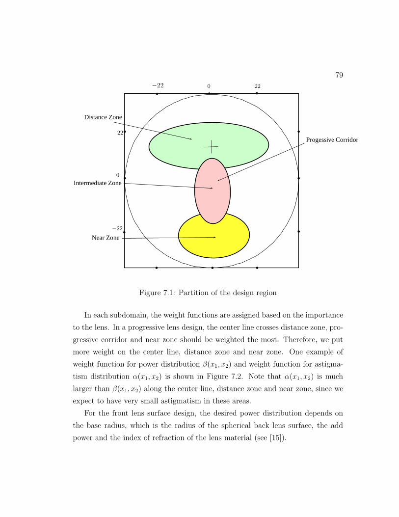
79
Distance Zone
Intermediate Zone
Near Zone
b
b b
b
bb
22
−22
0
b
b
b
b
b
b
−22 0 22
Progessive Corridor
Figure 7.1: Partition of the design region
In each subdomain, the weight functions are assigned based on the importance
to the lens. In a progressive lens design, the center line crosses distance zone, pro-
gressive corridor and near zone should be weighted the most. Therefore, we put
more weight on the center line, distance zone and near zone. One example of
weight function for power distribution β(x1, x2) and weight function for astigma-
tism distribution α(x1, x2) is shown in Figure 7.2. Note that α(x1, x2) is much
larger than β(x1, x2) along the center line, distance zone and near zone, since we
expect to have very small astigmatism in these areas.
For the front lens surface design, the desired power distribution depends on
the base radius, which is the radius of the spherical back lens surface, the add
power and the index of refraction of the lens material (see [15]).
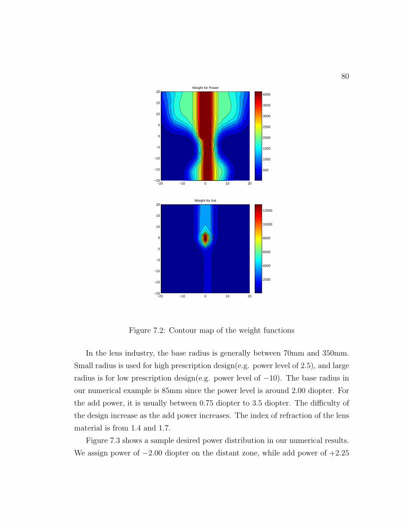
80
Weight for Power
−20 −10 0 10 20−20
−15
−10
−5
0
5
10
15
20
500
1000
1500
2000
2500
3000
3500
4000
Weight for Ast
−20 −10 0 10 20−20
−15
−10
−5
0
5
10
15
20
2000
4000
6000
8000
10000
12000
Figure 7.2: Contour map of the weight functions
In the lens industry, the base radius is generally between 70mm and 350mm.
Small radius is used for high prescription design(e.g. power level of 2.5), and large
radius is for low prescription design(e.g. power level of −10). The base radius in
our numerical example is 85mm since the power level is around 2.00 diopter. For
the add power, it is usually between 0.75 diopter to 3.5 diopter. The difficulty of
the design increase as the add power increases. The index of refraction of the lens
material is from 1.4 and 1.7.
Figure 7.3 shows a sample desired power distribution in our numerical results.
We assign power of −2.00 diopter on the distant zone, while add power of +2.25
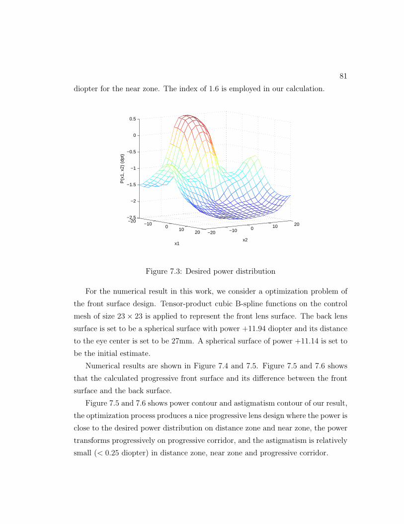
81
diopter for the near zone. The index of 1.6 is employed in our calculation.
−20−10
010
20 −20 −10 0 10 20
−2.5
−2
−1.5
−1
−0.5
0
0.5
x2x1
P(x
1, x
2) (
dpt)
Figure 7.3: Desired power distribution
For the numerical result in this work, we consider a optimization problem of
the front surface design. Tensor-product cubic B-spline functions on the control
mesh of size 23× 23 is applied to represent the front lens surface. The back lens
surface is set to be a spherical surface with power +11.94 diopter and its distance
to the eye center is set to be 27mm. A spherical surface of power +11.14 is set to
be the initial estimate.
Numerical results are shown in Figure 7.4 and 7.5. Figure 7.5 and 7.6 shows
that the calculated progressive front surface and its difference between the front
surface and the back surface.
Figure 7.5 and 7.6 shows power contour and astigmatism contour of our result,
the optimization process produces a nice progressive lens design where the power is
close to the desired power distribution on distance zone and near zone, the power
transforms progressively on progressive corridor, and the astigmatism is relatively
small (< 0.25 diopter) in distance zone, near zone and progressive corridor.

82
−40−20
020
40
−40
−20
0
20
4022
24
26
28
30
32
−40−20
020
40
−40
−20
0
20
402
4
6
8
10
Figure 7.4: Calculated Progressive Surface

83
−2
−1.75 −1.75
−1.75
−1.75
−1.5
−1.5
−1.5
−1.25
−1.25
−1.25
−1
−1
−1
−0.75
−0.75
−0.75
−0.5
−0.5
−0.5
−0.250 0.25
Power Contour of the designed lens
−20 −10 0 10 20−20
−15
−10
−5
0
5
10
15
20
−2
−1.75
−1.75
−1.5
−1.5
−1.5
−1.25
−1.25
−1.25
−1
−1
−1
−0.75
−0.75 −0.75
−0.5−0.250
0.25
Prescribed Power Contour
−20 −10 0 10 20−20
−15
−10
−5
0
5
10
15
20
Figure 7.5: Contour map of power of the designed lens and the prescribed power
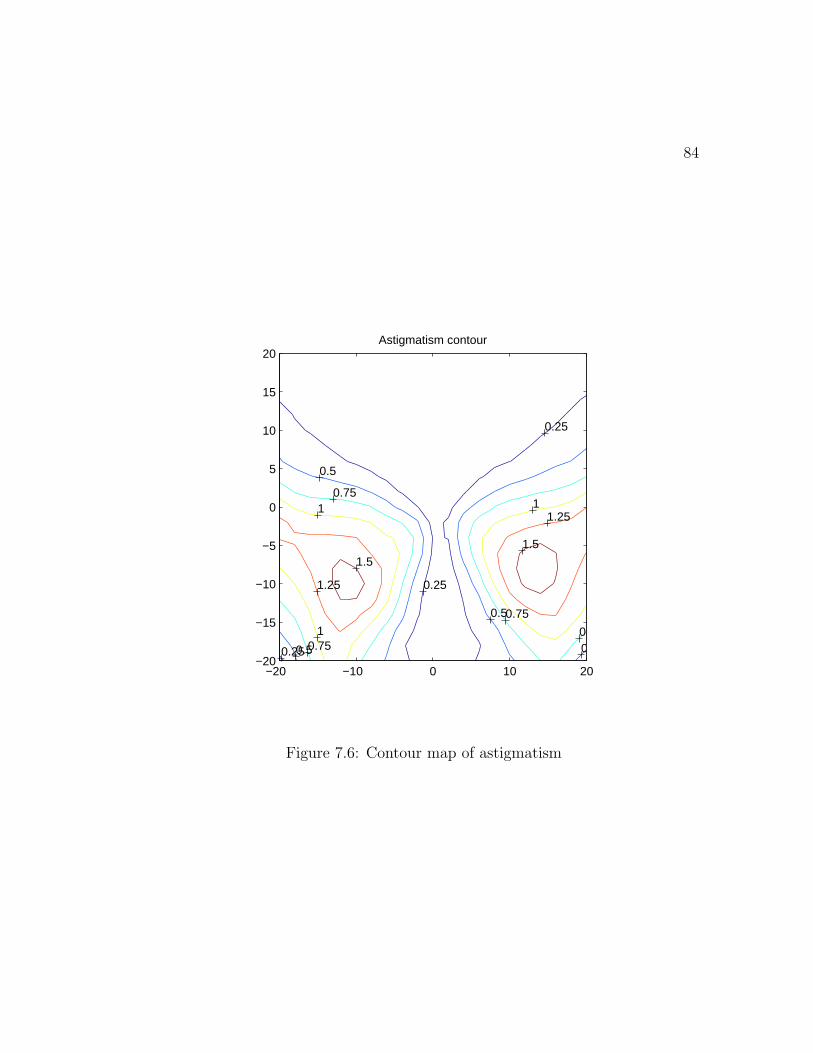
84
0.25
0.25
0.25
0.5
0.5
0.5
0.50.75
0.75
0.75
0.751
1 1
1.25
1.25
1.5
1.5
Astigmatism contour
−20 −10 0 10 20−20
−15
−10
−5
0
5
10
15
20
Figure 7.6: Contour map of astigmatism
Chapter 8
Discussion
In this work, we studied the problem of progressive addition lens design with
wavefront tracing method. The design problem is to obtaining a front lens surface,
or a back lens surface or both surfaces such that the power distribution of the
refracted wavefront is close to a desired power distribution and the astigmatism
of the refracted wavefront is minimized over the designated regions. When posed
as a variational problem, the design problem is a nonlinear optimization problem.
To evaluate power, astigmatism and higher order abberations of the refracted
wavefront, we developed new formulas of First Fundamental Form Coefficients,
Second Fundamental Form Coefficients and Third Order Surface Coefficients of
the wavefront on propagation in a homogeneous medium and on refraction at
a lens surface. With these formulas, a complete model of describing how the
curvature changes when a planar wavefront passing though a lens is obtained by
ray tracing method. The new formulas also allow for somewhat straight-forward
calculation of the gradients of the design objective.
To solve the problem numerically tensor-product B-splines are employed to
represent the surfaces. Several optimization methods for nonquadratic optimiza-
tion are considered, among them are the gradient method, Newton’s method and
the quasi-Newton. The quasi-Newton method is implemented in this work.
As an example, we deomonstrate our method on the problem of designing
85

86
a front progressive lens surface when the back surface is a spherical surface of a
fixed radius. In the calculation, weight functions are chosen so that the prescribed
power is close to the desired one in important areas of the lens while at the same
time astigmatism in these areas are made small. We obtained a lens with good
properties using our method.
Future research should focus on several improvements. First, there is a need to
speed up the computation. The evaluation of the cost function in the optimization
is necessarily complex. However, the wavefront in each gaze is independent and
thus a parallel approach is possible. Second, if we extend the design mesh to larger
size, say [−30, 30]×[−30, 30], which is the industrial standard for lens design mesh,
the memory needs for storing the Hessian or the approximate Hessian becomes
excessive so we should consider limited-memory Quasi-Newton methods. Third,
when we designing over a large region, the Hessian may become ill-conditioned.
This means that regularization methods must be considered. The ill-conditioning
may be explained by the sensitivity of the rays to small changes in the surface,
or rays that leave the region when the surface is perturbed. Finally, minimizing
second order aberrations should be considered in the future.
Overall, we believe that this work, in which the light propagation is accurately
described using geometrical optics, holds a lot of promise for the lens design
problem. With further development, the method presented here can potentially
find use in industrial lens design.

References
[1] T. Baudaut, F. Ahsbahs, and C. Miege. Multifocal ophthalmic lens. United
States Patent, 6102544, 2000.
[2] M. Born and E. Wolf. Principles of Optics-Electromagnetic Theory of Prop-
agation, Interference and Diffraction of Light. Pergamon Press, 1975.
[3] M. P. Do Carmo. Differential Geometry of Curves and Surface. Prentice-Hall,
1976.
[4] C. de Boor. Total positivity of the spline collocation matrix. Indiana Uni-
versity Journal of Math, 25:541–551, 1976.
[5] Carl de Boor. A Practical Guide to Splines. Springer-Verlag New York, Inc.,
1978.
[6] J. E. Dennis. Numerical methods for unconstrained optimization and nonlin-
ear equations. Englewood Cliffs, N.J. : Prentice-Hall, 1983.
[7] J. H. Gallier. Curves and surfaces in geometric modeling : theory and algo-
rithms. San Francisco, Calif. : Morgan Kaufmann Publishers, 2000.
[8] J. Kneisly II. Local curvature of wavefronts in an optical system. Journal of
The Optical Society of America, 54(2):229–235, 1964.
[9] D. Katzman and J. Rubinstein. Method for the design of multifocal optical
elements. United States Patent, 6302540, 2001.
87

88
[10] J. Loost, G. Greiner, and H.P. Seidel. A variational approach to progressive
lens design. Computer Aided Design, 30:595–602, 1998.
[11] J. Loost, Ph. Slusallek, and H.P. Seidel. Using wavefront tracing for the
visualization and optimization of progressive lens. EUROGRAPHICS’98,
17(3):c–255–265, 1998.
[12] D. Malacara. Optical Shop Testing. John Wiley and Sons, Inc., 1978.
[13] J. Nocedal and S. J. Wright. Numerical optimization. New York: Springer,
1999.
[14] J. Rubinstein and G. Wolansky. Wavefront method for designing optical
elements. United States Patent, 6655803, 2003.
[15] J. Sheedy, R. Hardy, and J. Hayes. Progressive addition lenses c measure-
ments and ratings. Optometry, 77:34–36, 2006.
[16] A. Sherman. On Newton-iterative methods for the solution of systems non-
linear equations. SIAM Journal on Numerical Analysis, 15:755–771, 1978.
[17] J. Wang. Design of progressive lenses-mathematical analysis and numerical
methods. UMI Microform 3058674, UMN Thesis, 2002.
[18] J. Wang, R. Gulliver, and F. Santosa. Analysis of a variational approach to
progressive lens design. SIAM J. Appl. Math., 64:277–296, 2003.
[19] J. Wang and F. Santosa. A numerical method for progressive lens design.
Mathematical Models and Methods in Applied Sciences (M3AS), 14:619–640,
2004.
[20] J. Wang, F. Santosa, and R. Gulliver. Multifocal optical device design. United
States Patent, 7044601, 2006.
[21] J. T. Winthrop. Progressive addition spectacle lens. United States Patent,
4861153, 1989.