Design of Partitions
39
Design of Partition: Transmission Loss Measurement Term Paper MEL314 This paper presents an overview on design of different types of partitions and the most important parameter that defines the effectiveness of a partition, that is, its transmission loss. The authors have tried to present how partitions can be designed to perform better under operating frequency ranges. 2013 Adityaraj Singh Thakur 2010ME10643 Aniruddh Vijaivargiya 2010ME10650 Jayendra Kashyap 2010ME10683 Sourav Sinha 2010ME10732
Transcript of Design of Partitions

Design of Partition:
Transmission Loss Measurement Term Paper MEL314 This paper presents an overview on design of different types of partitions and
the most important parameter that defines the effectiveness of a partition, that is,
its transmission loss. The authors have tried to present how partitions can be
designed to perform better under operating frequency ranges.
2013
Adityaraj Singh Thakur 2010ME10643
Aniruddh Vijaivargiya 2010ME10650
Jayendra Kashyap 2010ME10683
Sourav Sinha 2010ME10732

Table of Contents
Table of Figures ...................................................................................................................................... 3
1. INTRODUCTION .......................................................................................................................... 4
2. PARTITIONS: AN INTRODUCTION .......................................................................................... 5
3. THEORETICAL BACKGROUND ................................................................................................ 7
3.1 Transmission Loss (TL) .......................................................................................................... 7
4. MEASURING TRANSMISSION LOSS ........................................................................................ 9
5. SOUND TRANSMISSION CLASS ............................................................................................. 10
6. SOUND TRANSMISSION THROUGH ISOTROPIC PANELS ................................................ 11
6.1 Bending waves in isotropic panels ........................................................................................ 11
6.2 Panel Transmission Loss Behavior ....................................................................................... 14
6.3 Single leaf Transmission Loss .............................................................................................. 15
6.3.1 Davy’s Prediction Approach ......................................................................................... 16
6.3.2 Sharpe’s Prediction Approach: ..................................................................................... 17
6.4 Sandwich Panels ................................................................................................................... 19
6.5 Double Wall Transmission Loss ........................................................................................... 19
6.5.1 Sharpe’s Model ............................................................................................................. 20
6.5.2 Davy’s Model ................................................................................................................ 23
6.6 OTHER TYPES OF PARTITIONS ...................................................................................... 25
6.6.1 Multi Leaf partition ....................................................................................................... 25
6.6.2 TRIPLE WALL TRANSMISSION LOSS ................................................................... 25
7. SELECTION OF PARTITION ..................................................................................................... 26
8. COMPOSITE TRANSMISSION LOSS ....................................................................................... 28
9. FLANKING TRANSMISSION OF PANEL ................................................................................ 29
10. TEST EXPERIMENT ............................................................................................................... 30
10.1 Aim ....................................................................................................................................... 30
10.2 Apparatus used ...................................................................................................................... 30
10.3 Test set up and theory ........................................................................................................... 30
10.4 Results of Experiment ........................................................................................................... 33
10.5 Analysis................................................................................................................................. 36
11. CONCLUSION ......................................................................................................................... 37
12. REFERENCES ......................................................................................................................... 38
APPENDIX ........................................................................................................................................... 39

Table of Figures
Figure 1 Different Applications of partitions namely (a) Residential (partition between two rooms)
(b) Industrial (soundproofed control room) (c) Office (d) Field (isolating some machine).................... 5
Figure 2: Some examples of partitions with their STC ratings out of myriad possibilities. ................... 6
Figure 3: Transmission Loss through partition ....................................................................................... 7
Figure 4: Geometry of corrugated panel ................................................................................................. 8
Figure 5: Noise Reduction and Transmission Loss................................................................................. 9
Figure 7 Subjective equivalent for different STC's ............................................................................... 10
Figure 6: STC rating of panel ............................................................................................................... 10
Figure 8: Bending wave of panel .......................................................................................................... 11
Figure 9: Coupling of Acoustic Wave and the panel Flexural Wave (a) At and above the critical
frequency the panel radiates (b) At less than critical Frequencies the disturbance is local. the panel
does not radiate except at boundaries ................................................................................................... 13
Figure 10: Panel transmission loss behavior ......................................................................................... 14
Figure 11: Single leaf Transmission Loss Characteristic ...................................................................... 15
Figure 12: Geometry of a Corrugated Panel ......................................................................................... 16
Figure 13: Design Chart for estimating Transmission Loss of single Panel ......................................... 18
Figure 14: Design Chart for estimating Double Wall Transmission Loss (Sharpe 1973) .................... 22
Figure 15: Selection of partitions I ....................................................................................................... 27
Figure 16: Selection of Partitions II ...................................................................................................... 27
Figure 17: Design Chart for estimating Composite Panel Transmission Loss ..................................... 28
Figure 18: Flanking Transmission Path ................................................................................................ 29
Figure 19: Experiment Set-Up .............................................................................................................. 30
Figure 20: Smaller Enclosure Dimensions ............................................................................................ 32
Figure 21: Larger Enclosure Dimensions ............................................................................................. 32
Figure 22: Double Wall Enclosure with Glasswool .............................................................................. 32
Figure 23: Single Wall Transmission Loss (Smaller Enclosure) .......................................................... 34
Figure 24: Single Wall Transmission Loss (Larger Enclosure) ............................................................ 34
Figure 25: Double Wall Transmission Loss (Without Glasswool) ....................................................... 35
Figure 26: Double Wall Transmission Loss (With Glasswool) ............................................................ 35
Figure 27: Comparison of Transmission Loss for various Enclosures ................................................. 36

1. INTRODUCTION
This paper gives an overview of different types of partition designs. It elucidates the requirements on
part of a designer while designing a partition for a definite purpose. The authors have outlined the
methods of quantifying the acoustic performance of a partition through both experimental and
theoretical methods.
In the final part of this paper the authors have given an overview of an experiment that was performed
for studying the acoustic performance of different types of partitions.
2. PARTITIONS: AN INTRODUCTION
Sometimes noise source already exists and it becomes difficult to modify it as per the requirement.
For example in case of IC engines. In such cases it is required to modify acoustic transmission paths
without disturbing the running condition of source. Transmission is generally modified either through
barriers or enclosures or through partitions. But before designing the transmission path one should
carefully identify the dominating acoustic radiation source, whether it is airborne or structure borne
(generating from structures mechanically connected to source). Otherwise, whole design will turn out
useless without any decrease in sound levels.
This term paper aims at theoretical and experimental analysis of Single and Double leaf partitions for
airborne sound as well as measures to improve transmission loss. For proceeding with the analysis a
clear picture of transmission loss is required.
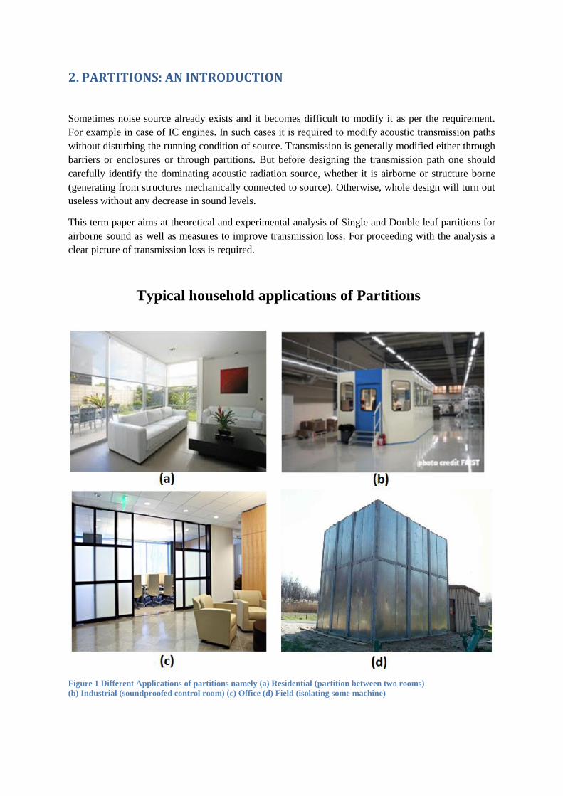
Typical household applications of Partitions
Figure 1 Different Applications of partitions namely (a) Residential (partition between two rooms)
(b) Industrial (soundproofed control room) (c) Office (d) Field (isolating some machine)

½ INCH GYPSUM BOARD – STC 28
SHEET BLOCK – STC 27
Figure 2: Some examples of partitions with their STC ratings out of myriad possibilities.
However, there can numerous combinations of the materials that have been used on the basis of their
thickness, air gap, material properties etc.

3. THEORETICAL BACKGROUND
Different types of partitions are available for different applications. Even for the same application,
markets offer a wide variety of partitions. So the pressing concerns of a designer or an user for a
partition should be based on two most important factors:
1. Strength of the partition:
The strength consideration of the partition should be a top priority because even if sound
isolation is a consideration, a strong partition is necessary for a safe, robust and durable
structure.
2. Acoustic performance of the partition: By acoustic performance of a partition one means
whether the partition is able to isolate the sound source from the receiver.
In this paper we will primarily focus on the acoustic performance of a partition. The acoustic
performance can be quantified as to how much incident sound energy on the partition from the source
side is actually transmitted onto the receiver side, in other words we need to calculate the transmission
coefficient of the partition and therefore its transmission loss.
3.1 Transmission Loss (TL)
When sound is incident upon a wall or partition some of it will be reflected and some will be
transmitted through the wall. The fraction of incident energy which is transmitted is called the
transmission coefficient . The transmission loss, TL (sometimes referred to as the sound reduction
index, Ri), is in turn defined in terms of the transmission coefficient,
τ = Itran/ Iin, where Iin is the incident sound intensity, Itran is the transmitted sound intensity……(1)
10 logTl ……(2)
Figure 3: Transmission Loss through partition
The transmission coefficient and thus the transmission loss will depend upon the angle of incidence of
the incident sound. Normal incidence, diffuse field (random) incidence and field incidence

transmission loss (denoted TLN, TLd and TL respectively) and corresponding transmission coefficients
(denoted τN, τd and τF respectively) are terms commonly used.
Noise Reduction (NR) : Let’s say sound level at one side of wall is measured to be 100 dB and on
other side it is 55 dB. Then it could be said that noise reduction is 45dB
Types of Transmission losses (based on
incident radiations)
Normal Incidence: As name
suggests incident field is normal to
partition
Diffuse field: Random field with
incident radiation from all the directions.
(θ varies from 0 to π/2 and υ varies from 0
to 2π )
Field Incidence : Incident
radiation having some limiting angle ϴL
(good approximation for finite partitions)
Figure 4: Geometry of corrugated panel

4. MEASURING TRANSMISSION LOSS
Method I:
It is generally measured using the standard specified in ISO 140–1978, Parts 3 and 4, AS1191–1985,
ASTM E336–1984. Revised standards might now be available for above standards. It is usually
measured in laboratory by placing the partition between two reverberant rooms namely source and
receiver room. Then mean space average sound pressure levels (sufficiently away from the source) is
measured in both source and receiver room. Difference in their levels is defined as noise reduction,
NR.
Final expression relating NR and TL :
………(3) Where Ap = Area of partition
Ap = Area of partition
= Avg. Absorption Coefficient of room
Method II:
Transmission loss of a partition can also be determined using single reverberant room for source and
free field for receiver. In diffuse field, incident power (π1) is calculated from the expression
,
where Pi is diffused field pressure in the source room, o is density of medium and c is velocity of
sound. Transmitted power is determined by measuring the average of the active sound intensity very
close (500 to 100 mm) to the panel on the receiving room side and multiplying it by area of partition.
Transmission coefficient is then ratio of transmitted to incident power.
This method is only used as laboratory research purposes and not mentioned in any standards.
Figure 5: Noise Reduction and Transmission Loss

5. SOUND TRANSMISSION CLASS
The question arises that how different partitions will be rated. To compare different types of
partitions, many criteria’s are introduced like 1) sound transmission class (STC), ISO’s standard,
Outdoor-Indoor Transmission Class (OITC) and STC was most common out of them.(ASTM E90–
66T)
STC contours normally consists of horizontal
segment from 1250 Hz to 4000 hz, increasing
middle segment by 5 dB from 400 to 1250 Hz
and increasing low frequency segment by 15 dB
from 125 to 400 Hz. STC rating of panels is
estimated by plotting its 1/3rd
octave band TL
and comparing it with the STC contours.
The STC rating of a partition is
determined by plotting the one-third octave
band TL of the partition and comparing it with
the STC contours.
`
Vertically shifting of the STC contour until these two criteria is
satisfied gives partitions STC rating. (Value of TL at 500 Hz frequency)
1. The TL curve cannot be more than 8 dB below the STC contour in any of the one-third octave
band.
2. Deficiencies sum below the TL curve of STC contour over the 16 one-third octave bands
cannot exceed 32 dB.
Figure 7 Subjective equivalent for different STC's
Suppose you are in a room next to one where two people are having a cnversation. According
to the construction of the wall and its accoustic performance, the STC illustrates what you can
hear.
Figure 6: STC rating of panel

6. SOUND TRANSMISSION THROUGH ISOTROPIC PANELS
6.1 Bending waves in isotropic panels
In solids, longitudinal waves can occur, as well as in liquids and gases. They have well-known
property that the particles vibrations are along or parallel to the direction of waves propagation. It is
also possible to find the excitation of transverse waves in solids due to the presence of shear force;
however, transverse waves hardly present in the media other than solid, i.e. liquids and gases. That is
mainly because the particles in other media cannot resist in shape deformation as the particles of solid.
Solid materials are capable of supporting shear as well as compressional stresses, so that in solids
shear and torsional waves as well as compressional (longitudinal) waves may propagate. In the audio-
frequency range in thick structures, for example in the steel beams of large buildings, all three types
of propagation may be important, but in the thin structures of which wall panels are generally
constructed, purely compressional wave propagation is of negligible importance. Rather, audio-
frequency sound propagation through panels and thus walls is primarily through the excitation of
bending waves, which are a combination of shear and compressional waves. They are significant not
merely because they are one of the most common types of waves in solids, but also due to the fact that
sound radiation are mainly contributed by them, that is due to the fact that the displacements of
bending waves are perpendicular to the directions of propagations and this nature means bending
waves lead to much more interactions between the structures and the adjacent medium, e.g. the most
common one, air, than the other waves do. Thus most of the energy transmitted to the adjacent
medium is by means of bending waves, i.e. bending waves are majorly responsible to radiations.
Isotropic panels are characterized by uniform stiffness and material properties. Bending waves in thin
panels, as the name implies, take the form of waves of flexure propagating parallel to the surface,
resulting in normal displacement of the surface. The speed of propagation of bending waves increases
as the ratio of the bending wavelength to solid material thickness decreases. That is, a panel’s stiffness
to bending, B, increases with decreasing wavelength or increasing excitation frequency.
The speed of bending wave propagation, CB, for an isotropic panel is given by the following
expression: 1
2 4
BB
Cm
(m/s) ………..(4)
Figure 8: Bending wave of panel

Thus, the wave speed for bending waves is frequency dependent. The different harmonics will travel
with different speeds i.e. a given waveform will change its shape overtime.
The bending stiffness, B, is defined as:
3
212(1 )
EhB
3
212(1 )
EhB
kg m2 s
-2 ……………..(5)
ω is the angular frequency (rad/s), h is the panel thickness (m), ρm is the material density, m=ρmh is
the surface density (kg/m2), E is Young’s modulus (Pa), ν is Poisson’s ratio and I′=h
3/12 is the cross-
sectional second moment of area per unit width (m3), computed for the panel cross-section about the
panel neutral axis.
There exists, for any panel capable of sustaining shear stress, a critical frequency (sometimes called
the coincidence frequency) at which the speed of bending wave propagation is equal to the speed of
acoustic wave propagation in the surrounding medium. The frequency for which airborne and solid-
borne wave speeds are equal, the critical frequency, is given by the following equation:
2
2c
c mf
B
π ………………………(6)
where c is the speed of sound in air.
the longitudinal wave speed, cL, for thin plates is given by:
2[ (1 )]L
m
Ec
m/……………………..(7)
Therefore the longitudinal wave speed may be written as:
12L
B
h mc
………………………..(8)
At the critical frequency, the panel bending wavelength corresponds to the trace wavelength of an
acoustic wave at grazing incidence. A sound wave incident from any direction at grazing incidence,
and of frequency equal to the critical frequency, will strongly drive a corresponding bending wave in
the panel.
Alternatively, a panel excited in flexure at the critical frequency will strongly radiate a corresponding
acoustic wave.
As the angle of incidence between the direction of the acoustic wave and the normal to the panel
becomes smaller, the trace wavelength of the acoustic wave on the panel surface becomes longer.
Thus, for any given angle of incidence smaller than grazing incidence, there will exist a frequency
(which will be higher than the critical frequency) at which the bending wavelength in the panel will
match the acoustic trace wavelength on the panel surface. This frequency is referred to as a
coincidence frequency and must be associated with a particular angle of incidence or radiation of the
acoustic wave. The frequency when bending waves become supersonic in a plate or a beam is called
the critical or coincidence frequency fc. Thus, in a diffuse field, in the frequency range about and
above the critical frequency, a panel will be strongly driven and will radiate sound well. However, the
response is a resonance phenomenon, being strongest in the frequency range about the critical

frequency and strongly dependent upon the damping in the system. This phenomenon is called
coincidence, and it is of great importance in the consideration of transmission loss.
At excitation frequencies below the structure critical frequency, the modes which are excited will not
be resonant, because the structural wavelength of the resonant modes will always be smaller than the
wavelength in the adjacent medium.
Lower order modes will be excited at frequencies above their resonance frequencies. As these lower
order modes are more efficient than the higher order modes which would have been resonant at the
excitation frequencies, the radiated sound will be higher than it would be for a resonantly excited
structure having the same mean square velocity levels at the same excitation frequencies. As
excitation of a structure by a mechanical force results in resonant structural response.
Figure 9: Coupling of Acoustic Wave and the panel Flexural Wave (a) At and above the critical frequency the panel
radiates (b) At less than critical Frequencies the disturbance is local. the panel does not radiate except at boundaries

6.2 Panel Transmission Loss Behavior
Figure 10: Panel transmission loss behavior
STL or are highly dependent on frequency. The STL behavior can be divided into three basic
Regions:
In Region I, at the lowest frequencies, the response is determined by the panel’s static stiffness.
Depending on the internal damping in the panel, resonances can also occur which dramatically
decrease the STL.
In Region II (mass-controlled region), the response is dictated by the mass of the panel and the curve
follows a 6dB/octave slope. Doubling the mass, or doubling the frequency, results in a 6 dB increase
in transmission loss.
In this region, the normal incidence transmission loss can be approximated by:
210log[1 ( ) ]2
soTL
c
……………….(9)
Where
w= sound frequency (rad/sec)
c =characteristic impedance of medium
S =mass of panel per unit surface area
The random incidence transmission loss is:
10log(0.23 )o oTL TL TL dB…………………………….(10)
In Region III, coincidence between the sound wavelength and the structural wavelength again
decrease the STL.

6.3 Single leaf Transmission Loss
At low frequencies, the transmission loss is controlled by the stiffness of the panel. At the frequency
of the first panel resonance, the transmission of sound is high and, consequently, the transmission loss
passes through a minimum determined in part by the damping in the system. Ultimately, however, at
still higher frequencies in the region of the critical frequency, coincidence is encountered. Finally, at
very high frequencies, the transmission loss again rises, being damping controlled, and gradually
approaches an extension of the original
mass law portion of the curve. The rise in this region is of the order of 9 dB per octave.
The resonance frequencies of a simply supported rectangular isotropic panel of width a, length b, and
bending stiffness B per unit width may be calculated using the following equation:
……….(11)
The lowest order (or fundamental) frequency corresponds to i=n=1. For an isotropic panel, putting
B(bending stiffness) into Equation (1) give the following:
…………….(12)
Figure 11: Single leaf Transmission Loss Characteristic

A very stiff construction tends to move the first resonance to higher frequencies but, at the same time,
the frequency of coincidence tends to move to lower frequencies.
The transmission coefficient for a wave incident on a panel surface is a function of the bending wave
impedance, Z, which for an infinite isotropic panel is (Cremer, 1942):
…………..(13)
where η is the panel loss factor and m is the panel surface density (kg/m2).
The diffuse field transmission coefficient, τd, is found by determining a weighted average for τ(θ,v )
over all angles of incidence using the following relationship:
………………(14)
Figure 12: Geometry of a Corrugated Panel
For isotropic panels, Equation (14) can be simplified to:
………….(15)
In practice, panels are not of infinite extent and results obtained using the preceding equations do not
agree well with results measured in the laboratory. However, it has been shown that good
comparisons between prediction and measurement can be obtained if the upper limit of integration of
Equation (15) is changed so that the integration does not include angles of θ between some limiting
angle and 90°.
6.3.1 Davy’s Prediction Approach
Davy (1990) has shown that this limiting angle θL is dependent on the size of the panel as follows:
…………..(16)

where A is the area of the panel and λ is the wavelength of sound at the frequency of interest.
Introducing the limiting angle, θL, allows the field incidence transmission coefficient, τF, of isotropic
panels to be defined as follows:
………….(17)
Performing numerical integration allows the field incidence transmission coefficient to be calculated
as a function of frequency for any isotropic panel, for frequencies above 1.5 times that of first
resonance frequency of the panel.
Further simplification gives the following expression for the mass law transmission loss of an infinite
isotropic or orthotropic panel subject to an acoustic wave incident at angle θ to the normal to the panel
surface:
…………….(18)
In the frequency range below ƒc:
………(19)
Where, …………….(20)
In the frequency range above ƒc:
………..(21)
In the frequency range around the critical frequency:
………(22)
It seems that Equation (22) agrees better with experiment when values for the panel loss factor, η,
towards the high end of the expected range are used. It is often difficult to decide which equation is
more nearly correct because of the difficulty in determining a correct value for η.
6.3.2 Sharpe’s Prediction Approach:
Sharp (1973) showed that good agreement between prediction and measurement in the mass law
range is obtained for single panels by using a constant value for θL equal to about 85°. In this case, the
field incidence transmission loss, TL, is related to the normal incidence transmission loss, TLN, for
predictions in 1/3 octave bands, for which Δƒ/ƒ=0.236, by:
………..(23)
The prediction scheme is summarized as following for estimating the transmission loss for single
isotropic panels. In the preceding equation, if the predictions are required for octave bands of noise

(rather than for 1/3 octave bands), for which Δƒ/ƒ=0.707, then the “5.5” is replaced with “4.0”. Note
that the mass law predictions assume that the panel is limp. As panels become thicker and stiffer, their
mass law performance drops below the ideal prediction, so that in practice, very few constructions
will perform as well as the mass law prediction.
Alternatively, better results are usually obtained for the octave band transmission loss, TLo, by
averaging logarithmically the predictions, TL1, TL2 and TL3 for the three 1/3 octave bands included
in each octave band as follows:
…….(24)
For frequencies equal to or higher than the critical frequency, Sharp gives the following equation for
an isotropic panel:
TL=20 log10[πƒm/(ρc)]+10 log10[2ηƒ/(πƒc)] (dB)……………….(25)
Figure 13: Design Chart for estimating Transmission Loss of single Panel
(a) A design chart for an isotropic panel. The points on the chart are calculated as follows:
Point A: TL=20 log10ƒcm−54 (dB)
Point B: TL=20 log10ƒcm+10 log10η−45 (dB)

The case for orthotropic panels has not been discussed here to avoid complexity.
Davy method generally is more accurate at low frequencies while the Sharp method gives better
results around the critical frequency of the panel.
6.4 Sandwich Panels
In the aerospace industry, sandwich panels are becoming more commonly used due to their high
stiffness and light weight. Thus, it is of great interest to estimate the transmission loss of such
structures. These structures consist of a core of paper honeycomb, aluminium honeycomb or foam.
The core is sandwiched between two thin sheets of material commonly called the “laminate”, which is
usually aluminium on both sides or aluminium on one side and paper on the other. One interesting
characteristic of these panels is that in the mid-frequency range it is common for the transmission loss
of the aluminium laminate by itself to be greater than the honeycomb structure. Panels with thicker
cores perform better than thinner panels at high frequencies but more poorly in the mid-frequency
range. The bending stiffness of the panels is strongly frequency dependent. However, once a model
enabling calculation of the stiffness as a function of frequency has been developed, the methods
outlined in the preceding section may be used to calculate the transmission loss.
Damping capacity of a device is energy dissipated in a complete cycle.
∆U= ∫Fd dx (26)
Loss factor =∆U/2πUmax
Loss factors, η, for these panels when freely suspended are frequency dependent and are usually in the
range 0.01 to 0.03. However, when included in a construction such as a ship’s deck, the loss factors
are much higher as a result of connection and support conditions and can range from 0.15 at low
frequencies to 0.02 at high frequencies.
6.5 Double Wall Transmission Loss
When a high transmission loss structure is required, a double wall or triple wall is less heavy and
more cost-effective than a single wall. Design procedures have been developed for both types of wall.
However, the present discussion will be focussed mainly on double wall constructions.
For best results, the two panels of the double wall construction must be both mechanically and
acoustically isolated from one another as much as possible. Mechanical isolation may be
accomplished by mounting the panels on separate staggered studs or by resiliently mounting the
panels on common studs. Acoustic isolation is generally accomplished by providing as wide a gap
between the panels as possible and by filling the gap with a sound-absorbing material, while ensuring
that the material does not form a mechanical bridge between the panels. For best results, the panels
should be isotropic.

In the previous section it was shown that the transmission loss of a single isotropic panel is
determined by two frequencies, namely the lowest order panel resonance ƒ1 and the coincidence
frequency, ƒc. The double wall construction introduces three new important frequencies. The first is
the lowest order acoustic resonance, the second is the lowest order structural resonance, and the third
is a limiting frequency related to the gap between the panels. The lowest order acoustic resonance, ƒ2
replaces the lowest order panel resonance of the single panel construction and may be calculated using
the following equation:
ƒ2=c/2L , where c is the speed of sound in air and L is the longest cavity dimension.
In literature, there are basically two models for predicting Transmission Loss:
Sharpe’s Model.
Davy’s Model.
6.5.1 Sharpe’s Model
The lowest order structural resonance may be approximated by assuming that the two panels are limp
masses connected by a massless compliance, which is provided by the air in the gap between the
panels. In practice, it is necessary to introduce an empirical factor of 1.8 into the equation to give
better agreement with existing data for ordinary wall constructions (Sharp, 1973).
The following expression (Fahy, 1985) is obtained for the lowest order cavity resonance, ƒ0, for
panels that are large compared to the width of the gap between them:
(27)
In Equation m1, and m2 are, respectively, the surface densities (kg/m2) of the two panels and d is the
gap width (m). The empirical constant, “1.8” has been introduced by Sharp (1973) to account for the
“effective mass” of the panels being less than their actual mass. Finally, a limiting frequency ƒℓ,
which is related to the gap width d (m) between the panels, is defined as follows:
……………(28)
The frequency for which airborne and solid-borne wave speeds are equal, the critical frequency, is
given by the following equation:
……………………….(29)
m is the surface density (kg/m2), B is the bending stiffness.
Frequencies ƒ2, ƒ0 , ƒℓ, ƒc1 and ƒc2 are important in calculating the TL.
For double wall constructions, with the two panels completely isolated from one another both
mechanically and acoustically, the expected transmission loss is given by the following equations
(Sharp, 1978):
………………(30)
In Equation, the quantities TL1, TL2 and TLM are calculated by replacing m in

TL=20 log10[πƒm/(ρc)]−5.5 (dB)…………………………..(31)
with the values for the respective panel surface densities m1 and m2 and the total surface density,
M=m1+m2 respectively.
Equation (30) is formulated on the assumption that standing waves in the air gap between the panels
are prevented, so that airborne coupling is negligible. When installing a porous material, care should
be taken that it does not form a mechanical coupling between the panels of the double wall; thus an
upper bound on total flow resistance of 5ρc is suggested or, alternatively, the material can be attached
to just one wall without any contact with the other wall. Generally, the sound-absorbing material
should be as thick as possible, with a minimum thickness of 15/ƒ (m), where ƒ is the lowest
frequency of interest.
The transmission loss predicted by Equation (30) is difficult to realize in practice. The effect of
connecting the panels to supporting studs at points (using spacers), or along lines, is to provide a
mechanical bridge for the transmission of structure-borne sound from one panel to the other. Above a
certain frequency, called the bridging frequency, such structure-borne conduction limits the
transmission loss that can be achieved, to much less than that given by Equation (30). Above the
bridging frequency, which lies above the structural resonance frequency, ƒ0, and below the limiting
frequency, ƒℓ, the transmission loss increases at the rate of 6 dB per octave increase in frequency.
The attachment of a panel to its supporting studs determines the efficiency of conduction of structure-
borne sound from the panel to the. A panel attached directly to a supporting stud generally will make
contact along the length of the stud. Such support is called line support and the spacing between studs,
b, is assumed regular. Alternatively, the support of a panel on small spacers mounted on the studs is
called point support; the spacing, e, between point supports is assumed to form a regular rectangular
grid. The dimensions b and e are important in determining transmission loss. The four possible
combinations of such attachment are: line-line, line-point, point-line and point-point. Of these four
possible combinations of panel support, point-line will be excluded from further consideration, as the
transmission loss associated with it is always inferior to that obtained with line-point support.
In the frequency range above the bridging frequency and below about one half of the critical
frequency of panel 2 (the higher critical frequency), the expected transmission loss for the three cases
is as follows (see Figure below). For line-line support (Sharp, 1973):
……………(32)
For point-point support:
………………(33)

For line-point support:
TL=20 log10m1+20 log10(ƒc2e)+20 log10ƒ +10log10[1+2X+X*X]−93 (dB)……….(34)
…………………………..(35)
Equation (32) seems to give very good comparison between prediction and measurement, whereas
Equation (33) seems to give fair comparison. For line-point support the term X is generally quite
small, so that the
term in Equation (34) involving it may generally be neglected. Based upon limited experimental data,
Equation (33) seems to predict greater transmission loss than observed. The observed transmission
loss for point-point support seems to be about 2 dB greater than that predicted for line-point support.
A method for estimating transmission loss for a double panel wall is outlined in Figure below. In the
figure consideration has not been given explicitly to the lowest order acoustic resonance,f2. At this
frequency it can be expected that somewhat less than the predicted mass-law transmission loss will be
observed, dependent upon the cavity damping that has been provided. In addition, below the lowest
order acoustic resonance, the transmission loss will again increase, as shown by the stiffness
controlled portion of the curve in Figure1.
The procedure outlined in Figure 2 explicitly assumes that the inequality, Mƒ>2ρc, is satisfied.
Figure 14: Design Chart for estimating Double Wall Transmission Loss (Sharpe 1973)
In the following, the panels are assumed to be numbered, so that the critical frequency, ƒc1, of panel 1
is always less than or equal to the critical frequency, fc2, of panel 2, i.e., ƒc1≤fc2; m1 and m2 (kg
m−2) are the respective panel surface densities, and d (m) is the spacing between panels. b (m) is the
spacing between line supports, while e (m) is the spacing of an assumed rectangular grid between
point supports. c and cL (m/s) are, respectively, the speed of sound in air and in the panel material,
and h is the panel thickness. η1, and η2 are the loss factors respectively for panels 1 and 2.
Calculate the points in the chart as follows:
Point A:
…….(36)
Point B:
fc2=0.55c2/cL2h2 (Hz)………………(37)

The transmission loss, TLB, at point B is equal to TLB1 if no sound absorptive material is placed in
the cavity between the two panels, otherwise TLB is the larger of TLB1 and TLB2, calculated as
follows:
TLB1=TLA+20 log10(ƒc1/ƒ0)−6 (dB)……………………..(38)
(a)Line-Line support:
……….(39)
(b)Line-Point support:
TLB2=20 log10m1e+40 log10ƒc2–99 (dB)………………….(40)
(c) Point-Point support:
………..(41)
Point C:
(a) fc2≠ƒc1, TLC=TLB+6+10 log10η2 (dB)…………………(42)
(b) ƒc2=ƒc1, TLC=TLB+6+10 log10η+5 log10η1 (dB)………………(43)
Point D: ƒ1=55/d (Hz)………………..(44)
The final TL curve is the solid line in the figure.
The preceding equations for a double wall are based on the assumption that the studs connecting
the two leafs of the construction are infinitely stiff. This is an acceptable assumption if wooden
studs are used but not if metal studs (typically thin-walled channel sections with the partition leaves
attached to the two opposite flanges) are used (see Davy, 1990).
6.5.2 Davy’s Model
Davy (1990, 1991, 1993, 1998) presented a method for estimating the transmission loss of a double
wall which takes into account the compliance, CM (reciprocal of the stiffness) of the studs. Although
this prediction procedure is more complicated than the one just discussed, it is worthwhile presenting
the results here. Below the mass-air-mass resonance frequency, ƒ0, the double wall behaves like a
single wall of the same mass and the single wall procedures may be used to estimate the TL.
Above ƒ0, the transmission from one leaf to the other consists of airborne energy through the cavity
and structure-borne energy through the studs. The structure-borne sound transmission coefficient for
all frequencies above ƒ0 is (Davy, 1993):
…………(45)
………………….(46)
where b is the spacing between the studs and for line support on panel 2:
…………………(47)
where ƒc1 is the lower of the two critical frequencies corresponding to the two panels and the
radiation efficiencies, σ1 and σ2 . Note that if the calculated radiation efficiency is greater than one in
Equation (47), it is set equal to one. The radiation efficiencies are calculated as for simply supported
panels, with the perimeter equal to the overall panel perimeter plus twice the length of all of the studs.
For point support on panel 2, the square root sign is removed from the last term in Equation (47) and
the “2” in the denominator is replaced with “4/π” (Fahy, 1985, pages 94–96). The analysis is
independent of whether panel 1 is point or line supported. In calculating ƒ0 for the Davy method, the
empirical factor of 1.8 in Equation (27) is not used.
For commonly used steel studs, CM=10−6
m2N−1 (Davy, 1990) and for wooden studs, CM=0.
However, Davy (1998) recommends that for steel studs, the compliance is set equal to 0 as for
wooden studs, and the transmission coefficient for structure-borne sound, τFc, is decreased by a factor
of 10 over that calculated using Equation (45) with CM=0. The units of mechanical compliance of the
studs are meters2 per N or displacement per N of applied force per unit length along the studs and in a
direction normal to the plane of the attached panels.
The field incidence transmission coefficient for airborne sound transmission through a double panel
(each leaf of area A), for frequencies between ƒ0 and 0.9fc1 (where ƒc1 is the lower of the two critical
frequencies corresponding to the two panels),
……………(48)
Where,
……………..(49)
Where,θL, is the limiting angle and it should not increase 80degrees.
In the above equations ƒci is the critical frequency of panel i (i=1,2), m1, m2 are the surface densities
of panels 1 and 2 and is the cavity absorption coefficient, generally taken as 1.0 for a cavity filled with
sound absorbing material, such as fibreglass or rockwool at least 50mm thick. At low frequencies, the
maximum cavity absorption coefficient used in the above equation should not exceed kd, where d is
the cavity width. For cavities containing no sound absorbing material, a value between 0.1 and 0.15
may be used for (Davy, 1998), but again it should not exceed kd. At frequencies above 0.9fc1, the
following equations may be used to estimate the field incidence transmission coefficient for airborne
sound transmission:
………….(50)
……………(51)
……………….(52)
q1=η1ξ2+η2ξ1…………..(53)
q2=4(η1−η2)…………(54)
The quantities η1 and η2 are the loss factors of the two panels and ƒ is the one-third octave band centre
frequency.
The overall transmission coefficient is:

………………(55)
The value of τF from Equation (31) is then used to calculate the transmission loss (TL).
Note that for frequencies between 2ƒ0/3 and ƒ0, linear interpolation between the single panel TL result
at 2ƒ0/3 and the double panel result at ƒ0 should be used on a graph of TL vs log frequency.
6.6 OTHER TYPES OF PARTITIONS
6.6.1 Multi Leaf partition
A multi-leaf partition essentially consists of a partition with two or more leaves of partitions made of
the same material that are connected together. The connection can be made in one of the three ways
mentioned below:
1. Rigid connection: Ina rigid connection the two leaves are glue firmly at all points on the
surface of the leaves
2. Flexible connection: In this type of connection the two leaves are glued or nailed together at
widely separated intervals (0.3m to 0.6m)
3. Visco-elastic Connection: This type of connection entails connecting the leaves through a
viscoelastic material like silicone rubber (example: silastic).
When the leaves are connected rigidly, they essentially act as a single leaf. Therefore the panel can be
considered to have a thickness equal to the sum of the thicknesses of all the leaves, and a surface
density equal to the total surface density of the leaves.
For the case of the flexible and the Visco-elastic connection, the two leaves essentially act as separate
leaves in terms of bending wave propagation.
Each of the leaves used in the multi-leaf partitions may again be composite leaves, which is basically
a leaf made of two or more layers of different materials that are rigidly bonded together. The critical
frequency of the composite leaf can then be calculated using the equation: 2 0.5/ (2 )*( / )c eff efff c m B
…….(56), where meff
is the effective surface density of the panel and
Beff
is the effective stiffness.
6.6.2 TRIPLE WALL TRANSMISSION LOSS
Recent work on the transmission loss through triple walls by Tadeu and Mateus (2001) has shown that
with the same total weight and total air gap, the transmission loss in a triple wall was not significantly
better than the double wall partition. However this they attributed to a cut-off frequency, above which
3D reflection occurs, to lie well beyond the range for typical panel separations. This cut-off frequency
can be calculated by the formula:
fco = c/2d, where c is the speed of sound and d is the air gap between two consecutive walls
It is however possible to achieve a marked improvement in sound transmission loss with a triple panel
above the cut-off frequency.

According a model proposed by Sharpe (1973), the double wall panel has better performance for
frequency range below 4f0 whereas the triple wall has better transmission loss for frequency range
below 4f0 , where f0 is the double panel resonance frequency given by: 2 0.5
0 1 2 1 21/ (2 )*(1.8 ( ) / ( ))f c m m dm m ,………………….(57) where m1 and m2 are the
surface densities of the two panels.
7. SELECTION OF PARTITION
The methods of experimentally determining the Transmission Loss characteristics of a partition or the
method of estimating the transmission characteristics of a partition through the different models
mentioned above are only possible when the designer has already manufactured a partition or has an
idea of how the partition needs to be designed.
However as a design engineer one needs to understand what factors affect a partition design and
performance and how they should be utilized for achieving the desired performance from a partition.
For any partition, we would not like it to go into structural resonance or act in the coincidence region,
since at these two regions, the sound transmission loss of a partition is the minimum and therefore the
very purpose of installing a partition in the first place gets defeated.
Therefore while designing a partition we have to keep in mind that the resonance frequency and the
coincidence frequency of the partition do not lie in the range of frequencies that the partition is likely
to encounter.
Therefore the structural resonance frequency of the partition should be kept as low as possible and the
coincidence region as high as possible. For general partitions the coincidence frequency is a value
high enough not to be encountered in general frequency exposures. However the problem lies with the
structural resonance frequency.
To drive down the structural resonance frequency the following methods can be adopted:
1. Increase mass on both sides of the panel
2. Widen the air cavity
3. Introduce acoustic isolation through sound absorbing materials in the air cavity
The first two of these methods can be used to decrease the structural resonance frequency of the
partitions, as evident from the formulae of the resonance frequencies.
However as a designer one is faced with certain constraints in designing the partition. The two most
important constraints of these are:
1. Mass of the partition
2. Space occupied by the partition
The mass of the partition is important from the standpoint of cost and space is important from the
standpoint of both functionality of the partition and its aesthetics.

Under these circumstances it is important to understand whether a single leaf, double leaf, triple leaf
or multi-leaf partition will be a better option from the standpoint of acoustic performance.
Figure 15: Selection of partitions I
The picture above shows the acoustic performance of a triple leaf partition, depending on its
configuration. It is seen that for the same mass when the cavity inside the triple leaf partition is
increased the performance of the partition is improved from “BAD” to “FAIR”. Further for the same
space when the second drywall is removed and the two smaller air cavities are coupled to form one
large air cavity the performance is further improved to “EXCELLENT”. This shows that for the same
mass and the same space a double leaf partition is far better than a triple leaf partition for the same
materials used.
This is further corroborated in the next picture.
Figure 16: Selection of Partitions II

It is seen that for the same mass and the same space, using a double leaf not only places more mass on
each drywall but also increases the cavity between the two walls. As we increase the number of
leaves, for same mass and same space the air cavity decreases and also the mass on each drywall
decreases, thus degrading the performance of the partition as a whole.
8. COMPOSITE TRANSMISSION LOSS
A partition wall may not be made of the same material even at the exposed surface. Therefore it is
important to consider the overall transmission coefficient of the partition, by considering the
transmission coefficients of the individual partition materials, with relative weights that will depend
on the relative surface area that each material is exposed with.
Therefore the overall transmission coefficient of the single wall partition with different materials
along its exposed surface is given by:
1
1
n
i i
i
n
i
i
S
S
, ……………….(58) where i=1,2,…,n are the number of different materials.
Therefore the transmission loss for the single partition made from different material is given by:
TL = -10log10 (τ)
If a partition consists of two elements
only, then the transmission loss
increment ᵟTL can be measure using
the following graph:
Here TL1 is the transmission loss if
the entire panel is made from element
of higher transmission coefficient and
TL2 is the transmission loss of the
panel if the entire surface is made
from element with lower transmission
coefficient. The area ratio is the ratio
of the areas of the panel made from
the two elements.
The graph shows elements of lower
transmission loss when incorporated
in a panel with high transmission loss
will adversely affect the transmission
loss characteristic of the entire wall.
Figure 17: Design Chart for estimating Composite Panel Transmission
Loss

9. FLANKING TRANSMISSION OF PANEL
Installing a sound partition that has a high transmission loss does not necessarily ensure isolation of
the sound source. One of the most important form of sound transmission from source room to a
receiver room is the case of flanking transmission.
Flanking transmission is essentially the sound that is transmitted not through the separating elements
but via other paths like:
1. Ceilings
2. Floors
3. Windows
4. Fixtures and outlets
5. Shared structural building components
6. Structural joints
7. Plumbing chases
The most important and critical
flanking transmission loss occurs
through the structural joints that are
used for placing the partition
between the source and the
receiver.
The effective transmission loss
through a partition should therefore
include the effects of flanking
transmission also. This can be
calculated from the following.
TLoverall = -10log10(10-TL
flank/10
+10TL/10
) dB…………………..(58)
Where TL is the transmission loss through the partition alone and TLflank is the combined effective TL
through all the flanking paths normalized to the area of the partition. The value of TLflank can be
calculated using the equation
TLflank = Dn,f – 10log10(10/A) dB, ………………(59)
where A is the area of the partition, and Dn,f is given by
Dn,f = L1 – L2 – 10log10(Sα/10) dB,…………………(60)
Where L1 and L2 are the sound pressure levels in the source and the receiver rooms with the receiver
level only due to the flanking effects, and Sα is the absorption area of the receiving room.
Figure 18: Flanking Transmission Path

10. TEST EXPERIMENT
10.1 Aim The objective of this experiment was to measure the transmission loss characteristic of different types
of panels.
10.2 Apparatus used Multi-directional sound source, Amplifier, Frequency Generator, Sound Level Meter, Sound
Enclosures.
10.3 Test set up and theory The standard method of determining sound transmission loss and therefore the sound transmission
characteristics of a panel or partition has already been mentioned in the previous sections. However
due to physical constraints of time, cost and skill, it was not possible to conduct the experiment to
measure sound transmission characteristics in the standard ASTM method.
The experiment that was conducted involved designing enclosures with walls similar to the design of
partitions walls. The insertion loss because of the enclosure was measured and from the insertion loss
the transmission loss of the partition was measured.
The following is the schematic of the test set-up.
Direct Field
Diffuse Field (1) Enclosure
Π1E ΠOE (2)
Multi Directional Sound Source Receiver
Isolator Hard Ground
Figure 19: Experiment Set-Up
Π1E = I1E * AE , where Π1E= Power emitted from the sound source inside the enclosure
= Dc* AE /4 I1E = Intensity of sound falling on the inner surface of the enclosure
= p12*AE/(4 0c) AE = Area of the inside surface of the enclosure exposed to the sound
D = diffuse field energy density on the inner surface of the enclosure
………………….(61) c = speed of sound, p1 = rms sound pressure inside the enclosure
0 = Density of air
Again the power transmitted through the walls of the enclosure to outside of the enclosure is given by:
ΠOE = τ* Π1E , where τ is the transmission coefficient of the walls of the enclosure
= τ*p12*AE/(4 0c) …………………….(62)

Therefore, we can write
LΠOE = Lp1 + 10log10AE - 6- TL ………..(63) {10log10 τ = -TL, 10log10(4) = 6}
Now
ΠOE = Io*4πr2 , where Io is the sound intensity from an omni-directional source
= p22*4πr
2 /( 0c*Qϴ), where p2 is the rms sound pressure at the receiver
Qϴ is the directionality of the sound source which here is 2 because of the
hard ground
……………………….(64)
Therefore we get,
LΠOE = Lp2 – 10log10(Qϴ /(4πr2 )), …….(65)
From (63) and (64) we get,
Noise Reduction (NR) = Lp1 – Lp2 = TL + 6 – 10log10(AE) – 10log10(Qϴ /(4πr2 )),………..(66)
Now if there was no enclosure the sound pressure level at the receiver in the direct field would have
been:
Lp2’ = LΠ + 10log10(Qϴ /(4πr2 )),
From (3) we get,
Insertion Loss
IL = Lp2’ - Lp2 = LΠ - Lp1 + TL + 6 – 10log10(AE) …..(67)
Now with the enclosure in place the sound pressure level inside the enclosure can be written as:
Lp1 = LΠ + 10log10(Qϴ /(4πri2
) + 4/RE) ……..(68), where RE is the room constant of the inside of the
enclosure given by
RE = SE *αavg /(1- αavg), where SE also includes the source surface area.
Now from (68) and (67) we get,
IL = TL + 6 - 10log10(AE) - 10log10(Qϴ /(4πri2 ) + 4/RE),
Considering that the total inside of the enclosure has a diffuse field we get,
IL = TL + 6 - 10log10(AE) - 10log10(4/RE)
IL = TL + 10log10 (SE *αavg /((1- αavg)* AE ))
This was the formula that was used for the calculation of the Transmission loss of the panel.
The test was carried out in an anechoic chamber to ensure that the receiver was placed in a direct
field. The sound was increased in frequency from 160 Hz to 16000 Hz and readings were taken at
1/3th Octave band Frequencies, without the enclosure at a distance of 1.5 m from the sound source at
60 cm above the ground.
The next set of readings were taken at the same position at the same frequencies, for three different
enclosure designs.

1. Single wall enclosure: This enclosure had a single wall built from 1.5 cm thick plasterboard.
The outside dimensions of the enclosure were as follows:
60 cm 60 cm
60 cm
Figure 20: Smaller Enclosure Dimensions
2. Double Wall Enclosure: This enclosure was basically two enclosures, one of top of the other,
therefore acting as a double wall enclosure. For this we used the single walled enclosure and
then the larger enclosure was built from 8mm thick plywood, with inside dimensions as
follows:
90 cm 90 cm
90 cm
Figure 21: Larger Enclosure Dimensions
This effectively left a gap of 15 cm on either of the 5 sides of the enclosure between the two walls of
the enclosure.
3. Double Wall with glass wool filling: In this type of enclosure the above double wall type
enclosure was used. The difference in this type of enclosure was that the inside surface of the
outer enclosure was covered with a 8 cm thick layer of glass wool.
Inner enclosure outer enclosure
glasswool
Figure 22: Double Wall Enclosure with Glasswool

In all the three types of enclosures to minimize the flanking transmission, the source was placed on
acoustic foam base to minimize the vibrations transmitted through the ground. Moreover the base of
each enclosure in contact with the ground was also lined with foam to minimize the panel vibrations
getting transmitted to the ground.
Here AE = 1.65872
SE = (AE + 0.3249 + 0.2827) m2
1
1
n
i i
iavg n
i
i
S
S
……………………………………..(69)
Here the surfaces consist of the inner surface of the enclosure, the hard ground, the machine outer
surface.
10.4 Results of Experiment
The following chart shows the results of the experiment conducted.
Frequency (Hz) Single Wall TL
(dB) : Smaller
Enclosure
Single Wall TL
(dB): Larger
Enclosure
Double Wall TL
(dB)
Double Wall TL
(dB)
160 21.0 33.6 37.8 50.9
200 29.8 19.1 48.0 53.2
250 33.8 31.7 42.3 47.6
315 42.6 41.8 52.7 57.3
400 29.3 25.5 49.5 56.2
500 37.8 16.3 49.9 55.2
630 24.9 6.2 42.1 46.9
800 24.7 31.5 38.8 44.3
1000 18.8 24.3 32.6 34.6
1250 20.1 20.0 25.9 32
1600 23.6 26.8 46.7 45.6
2000 26.4 24.7 35.5 42.8
2500 29.2 29.2 44.3 49.9
3150 32.3 26.1 41.0 56.4
4000 40.5 34.8 47.4 54.9
5000 23.5 36.1 36.7 45.3
6300 29.5 35.2 48.7 58.7
8000 33.2 34.3 43.5 44.9
10000 33.9 38.8 52.2 51.2
12500 23.8 27.6 43.8 43.7
16000 29.9 30.0 52.6 55.4

The following are the Transmission Loss characteristics of the Enclosures as follows:
Figure 23: Single Wall Transmission Loss (Smaller Enclosure)
Figure 24: Single Wall Transmission Loss (Larger Enclosure)
0.0
5.0
10.0
15.0
20.0
25.0
30.0
35.0
40.0
45.0
TL (
dB
)
Frequency (Hz)
Single Wall Transmission Loss (Smaller Enclosure)
0.0
5.0
10.0
15.0
20.0
25.0
30.0
35.0
40.0
45.0
TL (
dB
)
Frequency (Hz)
Single Wall Transmission Loss (Larger Enclosure)

Figure 25: Double Wall Transmission Loss (Without Glasswool)
Figure 26: Double Wall Transmission Loss (With Glasswool)
0.0
10.0
20.0
30.0
40.0
50.0
60.0
Double Wall Transmission Loss (without glasswool)
Both without glasswool Poly. (Both without glasswool)
0
10
20
30
40
50
60
70
TL (
dB
)
Frequency (Hz)
Double Wall Transmission Loss (with Glasswool)

Figure 27: Comparison of Transmission Loss for various Enclosures
10.5 Analysis
1. It is seen that for all the types of enclosures, there is an initial dip in the transmission loss,
which can be attributed to the decrease in the transmission loss near the panel resonance
frequencies.
2. After the first resonance frequencies, the transmission loss increases in coherence with the
mass law region. This is true for all the enclosures.
3. Again for all the enclosures we find that after the mass law range, the transmission loss
reduces over a certain region. This can be accounted by the coincidence region.
4. In the final graph we find that the transmission loss is more for the double wall enclosure over
the single wall enclosure. This shows that an air gap in the partition wall can significantly
increase the transmission loss characteristics of a partition. Moreover with the use of
glasswool, we also find that the transmission loss characteristics has improved slightly.
0.0
10.0
20.0
30.0
40.0
50.0
60.0
70.0
Freq
uen
cy
16
0
20
0
25
0
31
5
40
0
50
0
63
0
80
0
10
00
1
25
0
16
00
2
00
0
25
00
3
15
0
40
00
5
00
0
63
00
8
00
0
10
00
0
12
50
0
TL (
dB
)
Frequency (Hz)
Transmission Loss v/s Frequency
Smaller
Bigger
Both without glasswool
Both withglasswool
Poly. (Smaller)
Poly. (Bigger)
Poly. (Both without glasswool)
Poly. (Both withglasswool)

11. CONCLUSION
Partitions are installed in order to isolate the receiver from the sound source. Their applications rage
from household to industrial, office spaces to railway stations. For a specific application we can have
different types of partitions. However we need to qualify partitions depending on their performance.
In this respect apart from the strength considerations, the most important parameter that is useful in
qualifying whether a particular partition is suitable for a definite application is its acoustic
performance.
Acoustic performance of a partition is quantified by how much transmission loss the partition can
result in and this loss is a function of the incident frequency.
There are standard methods for measuring transmission loss of a partition experimentally. There are
also empirical relations based on different models to determine theoretically the transmission loss that
a particular partition can achieve. However for a designer the most important should be the
parameters that affect the transmission loss of a particular parameter and how he can modify these
parameters in order to achieve the desired acoustic performance of a partition. In this respect the study
of the partition design is of utmost importance.
However partitions alone cannot be of much significance if sound transmission can occur through
flanking paths. Therefore while designing a partition one should incorporate the elements of flanking
transmission also to design an effective partition.
Lastly, the experimental results that the authors have got from an experiment conducted to find
transmission loss of different types of panels are quite in coherence with theory. It also substantiates
some of the most important aspects of partition design, that is, inclusion of air gaps within leaves of
partition and use of sound absorbing materials for partitions. The transmission loss characteristic of
the partitions experimented are testament to the fact that transmission characteristics depend on
incident frequency and the trend that it shows are quite in coherence with available literature.

12. REFERENCES
[1] Bies David A., Hansen Colin H., Engineering Noise Control: Theory and Practice, Third Edition,
Spon Press, 2003.
[2] Kinsler, Frey, Coppens, Sanders, Fundamentals of Acoustics, Fourth Edition, John Wiley and Sons
Inc., 2000
[3] Xin F.X., Lu T.J., “Analytical Modelling of sound transmission through clamped triple panel
partition separated by enclosed air cavities”, European Journal of Mechanics A/Solids, 2011, No 30,
770-782
[4] Brekket A., “Calculation Methods for the Transmission Loss of single, double and triple
partitions”, Applied Acoustics, 1981, No 14, 225-240
[5] Wang J., Lu T.J., Woodhouse J., Langley R.S., Evans J., “Sound Transmission through
lightweight double-leaf partitions: Theoretical Modelling”, Journal of Sound and Vibration, 2005, No
286, 817-847
[6] Lee, Ih, “Significance of resonant sound transmission in finite single partitions” Journal of Sound
and Vibration, 2004, No 277, 881-893
[7] Supercrete Limited, “Acoustic Wall System Design Guide”, 2008
[8] http://www.soundproofingcompany.com
[9] http://www.soundproofingcompany.com
[10] http://www.soundisolationstore.com

APPENDIX
SPL (dB) no
enclosure
SPL (dB) Smaller
Enclosure
SPL (dB) Larger
Enclosure
SPL (dB) Double
Enclosure (w/o
glasswool)
SPL (dB) Double
Enclosure
(Glasswool)
114.4 98 85.4 81.2 63.5
113.7 89.1 99.8 70.9 60.5
108.6 81.1 83.2 72.6 61
116.3 80.1 80.9 70 59
107.2 84.9 88.7 64.7 51
103.7 73.3 94.8 61.2 48.5
94.9 78.6 97.3 61.4 48
97.3 83 76.2 68.9 53
97.1 90.8 85.3 77 62.5
96 88.1 88.2 82.3 64
105.6 94.2 91 71.1 60
105.8 91.2 92.9 82.1 63
111.5 94.3 94.3 79.2 61.6
110.1 89.8 96 81.1 53.7
111.6 82.9 88.6 76 56.7
99.2 87.8 75.2 74.6 53.9
94.7 77.3 71.6 58.1 36
81.7 60.6 59.5 50.3 36.8
81.2 59.4 54.5 41.1 30
71.7 60 56.2 40 28
80 62.2 62.1 39.5 24.6