IEEE TRANSACTIONS ON AUTOMATIC CONTROL, VOL. 53, NO. 2, 2008, PP. 257–272 1

Design of Low-bandwidth Spatially Distributed FeedbackDimitry Gorinevsky, Fellow, IEEE, Stephen Boyd, Fellow, IEEE, and Gunter Stein Fellow, IEEE,

Abstract—The paper considers a family of linear time-invariant and spatially-invariant (LTSI) systems that are bothdistributed and localized. The spatial responses of the distributedplant are localized in spatial neighborhoods of each location. Thefeedback computations are also distributed and the informationflow is localized in a spatial neighborhood of each location.The feedback is aimed at controlling spatial distributions ofvariables in the systems with a relatively low bandwidth in thetime direction. Such systems have many important applicationsincluding industrial processes, imaging systems, signal and imageprocessing, and others.

We describe a new method for designing (tuning) a certainfamily of low-bandwidth controllers for such plants. We considerLTSI controllers with a fixed structure, which is PID or similarlow-bandwidth feedback in time and local in spatial coordinates.Two spatial feedback filters, symmetric and with finite spatialresponse, modify the local PID control signal by mixing in theerror and control signals at nearby nodes. These two filtersprovide loopshaping and regularization of the spatial feedbackloop. Like an ordinary PID controller, this controller structureis simple, but provides adequate performance in many practicalsettings.

We cast a variety of specifications on the steady-state spatialresponse of the controller and its time response as a set oflinear inequalities on the design variables, and so can carryout the design of the spatial filters using linear programming.The method handles steady-state limits on actuator signals, errorsignals, and several constraints related to robustness to plantand controller variation. The method allows handling the effectsof boundary conditions and guaranteed closed-loop spatial ortime decay. It does appear to work very well for low-bandwidthcontrollers, and so is applicable in a variety of practical situations.

Index Terms—Distributed system control, multidimensional,optimization, PID, bandwidth, loopshaping

I. INTRODUCTION

THIS paper is on feedback control design in large dis-tributed array systems. Array signal processing is a ma-

ture field with well understood design and analysis methods;there are numerous practical applications. Array control (arrayfeedback) field is much less mature and is an emerging tech-nology. We consider array systems with spatially distributedfeedback.

Array control systems have been used in industrial processesfor a long time. Perhaps the most widespread industrialapplication is in control of flat sheet processes, such as paperor plastic sheet manufacturing, where linear arrays of up to300 actuators might be employed. Paper machine processes

D. Gorinevsky and S. Boyd are with Information Systems Lab, Stan-ford University, Stanford, CA 94305, USA, e-mail: gorin@stanford.edu;boyd@stanford.edu

G. Stein is with Honeywell Labs, Minneapolis, MN 55418, e-mail: Gun-terStein@aol.com

This work was in part supported by the NSF GOALI Grant ECS-0529426and AFOSR grant FA9550-06-1-0514

are very diverse. They use actuator arrays for boundary con-trol of turbulent pulp flow, thermal profile control, moisturecontrol, and other physical processes; see [23], [19], [32] andreferences there for more detail. The empirical models andproblem statements used in industry for control of flat sheetprocesses do not depend on the underlying physics and closelyresemble the formulation in this paper.

Other industrial applications of array control are related tothermal processing: in semiconductor manufacturing, crystalgrowing [1], and material heat processing. In these applica-tions, spatial profiles of temperature are controlled using arraysof heating elements. An iterative learning control of batchthermal processing can also be described as a 2-D system (onecoordinate is the local time in the batch and another the batchnumber) and leads to a closely related problem statement, see[16]. A cross-sample of industrial applications of distributedcontrol including a few thermal processes can be found in[13].

In active or adaptive optics applications, large 2-D ar-rays of actuators deform a reflecting surface of a mirror toachieve wavefront control. A deformable mirror control anal-ysis closely related to formulation in this paper is presented in[31] where further references can be found. A related area isshape control of large scale deformable reflectors for groundand space applications, e.g., see [22].

Future array control applications could rely on low-costmanufacturing of large arrays of actuators and sensors asMicro-Electro Mechanical Systems (MEMS). It might bepossible to have computing embedded with the actuators.Several futuristic aerospace applications were discussed in theliterature including micro-adaptive flow control using arraysof microactuators distributed over an airfoil or a channelboundary.

In addition to the mentioned control applications, distributedfeedback is important in estimation problems. In systemstheory, estimation is dual to control, hence, the similarity inthe feedback analysis and design. The distributed estimationcan be encountered in processing data described by a seriesof images, such as in video processing, medical image pro-cessing (computational tomography, MRI, ultrasound imaging,etc), remote earth observation, nondestructive evaluation ofmaterials and structures, and more. The distributed estimationis closely related to solution of distributed inverse problemssuch as deblurring in image processing and grid methods forsolving partial differential equations. Formulations of imageprocessing and multidimensional filtering problem related tothis paper and further references could be found in [17], [20].

In this paper we assume that the distributed arrays are largeand make a regular spatial pattern. A fundamental technicalapproach to analysis of such systems is by assuming that thearrays have an infinite spatial extent (or are circulant). In that

2

case, an array can be modeled as a multidimensional systemand analyzed by changing from spatial coordinates to spatialfrequencies. Explanation and justification of spatial frequencytransforms are available in many signal processing texts andpapers including [4], [7] as well as in several image processingtextbooks. A relatively recent control-oriented discussion canbe found in [2]. If (closed-loop) responses decay fast enoughspatially, an infinite-array multidimensional system model canbe used with a finite array and boundary effects are limited.This is discussed further in more detail.

Modern control-theoretic approaches to analysis and designof feedback in large (or infinite) distributed systems withregular array structure were proposed and explored in anumber of publications. The most relevant to this paper are [3],[10], [11], [12], [21], where further references can be found.Most of this work is focused on design of high-performancespatially invariant feedback control systems, with performanceand robustness guarantees. Modern control design methods,such as linear matrix inequalities and mu-analysis are appliedto the distributed systems

Practical use of advanced control-theoretic approaches islimited, even for usual lumped system. Herein, we pose lessambitious control-theoretical goals in the hope of developingmethods that are easier to apply in practice; we focus on tuningmethods for distributed generalizations of low bandwidth PIDcontrollers. In practice, more than 90% of the control loopsuse PID, or PI, or PD, or P controllers. Since this is truefor usual, lumped, systems there is a hope that a simpledistributed generalization of a PID controller could satisfy theneeds of most array feedback applications. Realization of thisvision requires easily understood methods for controller tuning(design within the given simple structure).

Lumped systems with PID control usually have a decayingopen-loop response. Less forgiving systems might requireadvanced control approaches, but are a minority in practice.We assume that a response of the distributed system decaysin time and in space. This is the case in existing practicalapplications of array control. For such systems distributedPID-type control should be adequate.

There is substantial body of control-theoretical work ana-lyzing PDE models. Our work has a different flavor. IndustrialPID control design and tuning typically relies on basic modelsacquired in an simple identification test. Similarly, we describea distributed system by an empirical spatial and time response;see [19] for an example of industrial application where suchresponses are directly identified. The PDE models might ormight not be available.

In industrial array control (e.g., industrial cross-directionalcontrol of paper machines or temperature control), practition-ers usually start from attempting decoupled zonal control.Each zone would include an actuator (or a few) and will becontrolled independently of others. If there is a substantialinteraction between the zones, this simple approach is notfeasible. Spatial filtering of the feedback loop signals becomesnecessary. This paper considers a loopshaping approach to se-lecting the spatial filters such that the performance, robustness,and other specifications are satisfied (if this is possible).

An approach closely related to ours, but less automated, is

spatial loopshaping design (or tuning) of a distributed con-troller, as discussed in [32], [33]. The localized controller in[32], [33] is obtained by designing a non-localized controller,which is then truncated to provide a localized controller.Herein we assume a simple localized controller structure onthe outset and develop a formal design method that allowsaccommodating many important engineering specifications forcontroller design.

Since the controller structure is assumed at the outset,the solution pursued in this work is not completely general.This enables us to achieve a rather complete solution of theproblem.

In this paper, we consider a spatially distributed systemanalog of low-bandwidth PID control. A standard digital PIDcontroller uses three values of the plant output (current, pastand the integral) for computing the control. In a similar way,our ‘spatial PID’ controller uses data from a few neighboringarray cells. Such control is relatively simple to implementcomputationally. For centralized implementation of the arraycontrol, simplifying computations needed for hundreds orthousands of actuators might be critical. The same algorithmscan be conveniently implemented in an array of distributed em-bedded processors. Parallel processing makes computationalperformance less of an issue but constraints on communicationbetween the processors become important; local communi-cation with the nearest neighbors can be performed mostefficiently, see [28].

Like an ordinary PID controller, the distributed controllerstructure considered in this paper, provides adequate per-formance in many, or even most, practical situations. Thiswas demonstrated in a number of applications. Also like anordinary PID controller, it is not meant to achieve a limit ofpossible performance; it is meant to be adequate, after propertuning, in many practical cases.

An ordinary PID control implicitly assumes that the plantdynamics can be approximated as a first-order system. Theproposed distributed controller is based on two such assump-tions. First, that the space and time dynamics are separable.The second is that integrator dynamics are dominant in theclosed loop.

The contribution of this paper is in formulating the spatiallydistributed controller design (tuning) problem as a convexoptimization problem. Localized spatial (FIR) operators areassumed at the outset, and the main engineering specifica-tions are accommodated within a linear programming (LP)optimization framework. This allows for a computationallyefficient and conceptually clean one-shot solution for theoptimal FIR weights in the controller. We show how formalspecifications for performance, robustness, time decay, spatialdecay, and some others closed-loop characteristics can beincorporated into such LP-based design.

We will see that the conversion of the problem to an LP ispossible because the spatial responses considered are symmet-ric. This makes the spatial transfer functions (numerator anddenominator) real and enables us to convert linear fractional(closed-loop) design constraints into linear constraints. Thesame trick does not work in the absence of symmetry.

The idea that symmetry of a pulse response leads to a

3

real transfer function, and therefore limits on the frequencyresponse can be expressed as linear inequalities, is not new;it is the basis of linear programming based design of sym-metric FIR filters for signal processing applications, whichhas been done at least since 1969 (see [5, p. 380]). In thispaper, however, we consider closed-loop expressions, whichare linear fractional expressions in the FIR filter weights. Thelinear fractional expressions in filter design were cast as LPproblems, e.g., see [8], [14], [30]. However, to the best ofthe authors’ knowledge, this has not been done in a feedbackcontrol design context before.

II. PROBLEM STATEMENT

Consider a distributed system consisting of an array ofidentical cells. For each cell there is a scalar control handle uand a scalar feedback measurement y. There is also interactionbetween the cells in the sense that will be explained further inthe paper. Though there are several obvious ways to generalizethe analysis and design of this paper to cells with multipleinputs and outputs, we assume SISO (single-input singleoutput) cells for the sake of presentation clarity. Many practicalapplications, in particular all of the applications mentioned inIntroduction involve arrays with SISO cells.

To explain the motivation for the system model and con-troller structure considered in this paper, we will introduce aseries of increasingly complex models and controllers for suchsystem. The models and controller structure choice are guidedby engineering considerations auxiliary to mathematical anal-ysis. At the same time, we present quite rigorous analysis anddesign of the control loop for the formulated equations.

A. SISO model

Let us start from the simplest model and control law. Anapproach that a practitioner would initially attempt using for anarray system is to assume that there is no cross-cell interactionsuch that each cell can be controlled separately. The interactionis attributed to model uncertainty. The idea is that if thedesigned feedback loop is sufficiently robust, it would workas desired despite the presence of the spatial interaction.

If the cells are identical and do not interact, it is sufficientto consider a single cell. We assume that the output signal yof the cell is related to the control (input) signal u as

y = g(z−1)u + d, (1)

where d is the disturbance input, z−1 is a unit delay operatorand g(z−1) can be both considered as a system discretetransfer function and a dynamical response operator.

We assume that a robust (low-bandwidth) feedback is usedto control the output of the SISO loop (1) towards the setpointyd. The control law has the form

u = z−1u− z−1c(z−1)(y − yd), (2)

The controller c(z−1) is in the velocity form to emphasizethe presence of an integrator to counter slow changing andsteady state disturbance. Practically used industrial controllersusually include an integrator as assumed in (2). This includesa PI or PID controller (considered in the examples examples

of Section III-A and Section V), or a Dahlin controller(discrete-time Smith predictor), which is used in paper webmanufacturing control. We assume that the plant responsemight be instantaneous, i.e., g(z−1) in (1) is proper but mightbe not strictly proper. There is no feedthrough in the loop,however, and that is reflected by the unit delay operator z−1

shown at the feedback term in (2).The closed loop transfer function representation of the

system (1), (2) has the form

y =z−1c(z−1)

1− z−1 + z−1c(z−1)g(z−1)yd

+1− z−1

1− z−1 + z−1c(z−1)g(z−1)d (3)

In what follows, we assume that the closed loop transferfunctions in (3) are stable and provide gain and phase marginsto accommodate large uncertainty. Yet, in many practicalapplications the cell interaction is significant and cannot besimply attributed to the modeling uncertainty. More detailedmodeling and control design aimed at such applications arepresented below.

B. Separable two-dimensional plant model

In this paper, an array control system is modeled as alinear time-invariant spatially-invariant (LTSI) system. Weassume that the array cells make a regular spatial patternand that interaction between the neighboring cells repeatsitself from cell to cell up to the respective spatial shift. Amore in-depth description of LTSI control systems can befound in [2], [11]. An LTSI model allows for an efficientmultidimensional frequency-domain analysis of the problem.The analysis involving spatial frequencies can be consideredas modal analysis of the system dynamics, since the spatialsinusoids are the eigenmodes of a spatially invariant system[2].

An LTSI model does not consider boundary effects presentin a finite array (unless it has a circulant structure). Boundarycondition issues (which arise when the true plant and controllerare not spatially infinite) can be integrated into the frameworkdescribed herein as a deviation from the LTSI model, see [24],[26]. The boundary effects are closely related to the closed-loop spatial response decay, which is further considered as oneof the important formal design specifications. Such handlingof boundary conditions in Subsection 3.4 is in fact one of themajor contributions of this paper.

Consider a two-dimensional (2-D) distributed system evolv-ing in the integer time t = 0, 1, . . . and with an integerspatial coordinate x = . . . ,−1, 0, 1, . . . indexing the actuatorcells. The (scalar) actuator or control signal will be denotedu = u(t, x), which is the control applied by actuator numberx in the array, at time t. The (scalar) process output isy = y(t, x), where one measurement per actuator, and pertime sample, is assumed. A general input-output model of anLTSI plant has the 2-D convolution form

y(t, x) =∞∑

k=0

∞∑n=−∞

h(t− k, x− n)u(k, n), (4)

4

where h(t, x) is the system 2-D impulse response function, orsystem Green’s function.

We will assume a separable plant model, which has theform

h(t, x) = ht(t) hx(x), (5)

where ht(t) is the plant time impulse response, and hx(x) isthe plant spatial impulse response. We assume that ht is causal,i.e., ht(t) = 0 for t < 0. We will also assume that the plantis spatially symmetric, which means that hx(−x) = hx(x).(The same methods work for plants that are spatially anti-symmetric, i.e., satisfy hx(−x) = −hx(x).)

The analysis to follow uses a 2-D transfer function ofthe plant obtained by computing a z-transform of the pulseresponse (5). This transfer function has the form H(z, λ) =g(z−1)G(λ), where g(z−1) is the z-transform of the dy-namical impulse response ht(t) in (5) and G(λ) is a spatialtransfer function computed as the (two-sided) z-transform ofthe spatial impulse response (Green function) hx(x). Theplant is assumed stable and the spatial response absolutelysummable (spatially stable). This means g(z−1) is analyticinside the unit circle |z| ≤ 1 in the complex plane, and G(λ)is analytic inside an annulus r ≤ |λ| ≤ r−1, where 0 < r ≤ 1.

The separable 2-D plant model is y = g(z−1)G(λ)u. In thismodel z−1 can be interpreted as a unit time delay operator andλ as a unit positive spatial displacement operator. We assumethat g and G are scaled so g(1) = 1, i.e., the time transferfunction g is normalized to have unit static gain. The assumedspatial symmetry implies that the spatial transfer function Gis real for |λ| = 1. (If the plant were spatially anti-symmetric,then G would be pure imaginary for |λ| = 1.)

Separable models are applicable in many distributed systemswhere actuator dynamics or sensor dynamics or dynamics ofa fixed dynamical filter are dominant. These dominant timedynamics are described by the time response ht(t) while hx(x)gives the steady-state spatial response shape. Models of theform (5) are used in many practical applications of arraycontrol discussed in Introduction.

A separable model (5) might be also obtained as an ap-proximation of a general impulse response. As an example,consider a distributed system described by a heat equation

∂2y

∂x2=

∂y

∂t+ ay + u, (6)

where x ∈ < is spatial coordinate, t ∈ <+ is time, y = y(t, x)is the temperature, u = u(t, x) is the control input, and ais a thermal loss factor. The actuation and measurement areconcentrated (as δ-functions) at integer coordinates. An input-output map of the system can be represented in the form (4)with the impulse response (Green function of (6)) being

h(t, x) = e−ta(4πt)1/2e−x2/(4t), (7)

where t > 0 and x are integers; we assume that there is aone sample delay between the measurement and control sothat h(t = 0, x) = 0. We assume that a > 0, which meansthe system dissipates the heat and the impulse response (7)exponentially decays with time. This is the case for distributed

heating control applications in papermaking, manufacturing,materials processing, and semiconductors.

The response (7) is not separable. Yet it can be approxi-mated as such. Consider the argument domain DL = {t, x :(t = 0, 1, . . . , 2L+1; x = −L, . . . , L)}. For large enough L,the impulse response is vanishingly small outside the domainDL. Inside DL, the values h(t, x), {t, x} ∈ DL couldbe considered as entries of a matrix HL. A singular valuedecomposition of HL has the form

h(t, x) =2L+1∑

k=1

gk(t)σkhk(x), (8)

where gk(·) and hk(·) correspond to the left and right singularvectors of HL respectively, and σk is the respective singularvalue. A separable model (5) can be obtained as a truncationof (8) with ht(t) = σ1g1(t) and hx(x) = h1(x). If the firstsingular value is much larger than the rest, the approximationis accurate. This holds in many applications.

−25 −20 −15 −10 −5 0 5 10 15 20 250

0.1

0.2

0.3

0.4

SEPARABLE SPATIAL RESPONSE hx(x)

SPATIAL OFFSET x

0 20 40 60 80 1000

0.1

0.2

0.3

0.4

TIME DELAY t

SEPARABLE TIME RESPONSE ht(t)

FIRST SINGULAR VECTOREXPONENTIAL FIT

Fig. 1. Separable approximation of the heat equation response.

Assume a = 0.05 and L = 25. For the response (7) the firstfew singular values σk in (8) computed for the domain D25

are: 0.8668, 0.2636, 0.0931, 0.0341, 0.0126, 0.0046, 0.0016.The obtained spatial response hx(x) = σ1g1(t) and timeresponse ht(t) = h1(x) of the separable approximation areshown in Figure 1 as solid lines. The dashed line in thelower plot is a least square fit of a first-order time responsemodel (exponential response). An L2 error for the separableapproximation given by the ratio of the second and the firstsingular values is about 30%. However, as discussed furtherin the paper, an H∞ approximation error (a maximal errormagnitude over spatial and dynamical frequencies) is in factimportant for the analysis. This error is just 22%, much smallerthan the 33% H∞ robustness specification implemented in thedetailed design example of Section IV.

C. Multidimensional model

We will further consider a generalization of the just intro-duced separable model to a larger number of spatial dimen-sions.

5

Consider now a multidimensional system with n spatialcoordinates and time. With some overload of notation denotethe integer coordinate vector x = [x1 . . . xn]T . The cells inthe n-D array have control inputs u = u(t, x) and outputsy = y(t, x). We assume that the system has a separableimpulse response h(t, x) = ht(t)hx(x) and introduce thespatial operator

G(λ) =∞∑

x1=−∞. . .

∞∑xn=−∞

λx11 · · ·λxn

n hx([x1 . . . xn]T ), (9)

where λ = [λ1 . . . λn]T is the vector of the Laplace indeter-minates. As usual, an indeterminant λk can be interpreted aseither complex variable or a unit shift operator for the spatialcoordinate xk. This should be clear from the context.

With an overload of notation, the plant model used in thecontrol design and analysis has the form

y = g(z−1)G(λ)u + d, (10)

where d = d(x) is a static disturbance. The earlier considered2-D model is a special case of the multidimensional model(10) for n = 1.

We assume that the system spatial response hx(x) issymmetric (or anti-symmetric) in each of the variablesx1 . . . xn, such that either hx([x1 . . . − xk . . . xn]T ) =hx([x1 . . . xk . . . xn]T ) or hx([x1 . . . − xk . . . xn]T ) =−hx([x1 . . . xk . . . xn]T ). Denote the spatial frequencyvectors

ν = [ν1 . . . νn]T , eiν = [eiν1 . . . eiνn ]T

The symmetry (anti-symmetry) assumption means that thenon-causal transfer function G(eiv) is real (or purely imag-inary).

D. Control problem

We are interested in low-bandwidth control of the mul-tidimensional plant (10). The goal is to cancel the steady-state error in reaching the desired spatial profile yd(x). Theseparable model (10) is an extension of (1). Consider now aseparable controller that extends (2) in a similar way.

u = z−1u− z−1c(z−1)K(λ)(y − yd), (11)

where c(z−1) describes the controller time-dynamics. Thefunction of the spatial operator K(λ) is to improve theclosed-loop system response by compensating for the spatialinteraction effects reflected by the operator G(λ) in (10).

We now consider the closed-loop dynamics for the system(10)–(11). As discussed in more detail in [2], an LTSI systemcan be diagonalized by the spatial sinusoids. By substitutingλ = eiν we obtain the modal dynamics for the spatialfrequency ν. With some overload of notation, the controlupdate dynamics for the mode at frequency ν are

zu(t, ν) = u(t, ν)−K(eiν)G(eiν)g(z−1)c(z−1)u(t, ν)−K(eiν)c(z−1)[d(ν)− yd(ν)], (12)

where yd(ν) is a Fourier transform of yd(x)

yd(ν) = (2π)−n∑x1

. . .∑xn

yd(x)eiν1x1 . . . eiν1xn ,

and d(ν) is a Fourier transform of d(x).At high spatial frequencies, where G(eiv) ≈ 0, the actua-

tion signal might experience unlimited growth. In control ofindustrial distributed processes, this effect is known as actuatorpicketing. To see this, suppose the plant gain G(eiν) is zeroat some spatial frequency ν. The dynamics (12) at this spatialfrequency can be approximated as

zu(t, ν) = u(t, ν)−K(eiν)c(z−1)(d(ν)− yd(ν)).(13)

The second term in the r.h.s. (13) does not depend on controlu. However small the controller gain K(eiν) is, the integratorin (13) will keep adding the error until the feedback signalbecomes extremely large. The described situation is neverencountered in ‘normal’ PID control. This is because the plantgain is always nonzero as a precondition of system design forimplementation of closed-loop control. In a distributed system,plant gain might be zero for some modes while other modesare perfectly controllable.

The problem can be resolved by modifying the controller(11) for out-of-band control at frequencies where |G(eiν)| ¿1. At these frequencies, the compensation of the error y − yd

is not possible and the control convergence is most important.It can be achieved by using a controller structure given by

u = z−1u− z−1c(z−1)K(λ)(y − yd)− z−1S(λ)u (14)

The first two terms in (14) have the same form as in (11). Thethird term introduces an additional degree of freedom for theand can be interpreted as a regularization term. The spatialoperator S(λ) introduces an integrator leakage term enforcingthe out-of-band control convergence.

The regularization term is the best understood in relation tothe system steady-state. It prevents an attempt to compensatean error at spatial frequencies where a small plant gaincould lead to control inputs growing excessively large. Thiscorresponds to a regularized inversion of an ill-defined plant[34]. Controllers of the form (14) have been used in webmanufacturing processes [23], [15], [32].

We will assume that the controller, like the plant, is spatiallysymmetric, i.e., K and S are symmetric FIR filters; K(λ) andS(λ) are real for |λ1| = . . . = |λn| = 1. (For a plantwhere spatial response is anti-symmetric in some coordinates,we choose K anti-symmetric in the same coordinates andsymmetric S.)

The main problem is to design the spatial operators K(λ)and S(λ). We assume that the spatial filters K(λ) and S(λ)are FIR operators, which implies that the controller (14) isspatially localized; the control signal u(t, x) is computed basedon only a finite number of error and actuator signals, at nearbyactuator cells. This reflects important communication andcomputing constraints. For a centralized controller (finite butlarge array) FIR operators K and S can be implemented withhigh computational efficiency as convolution kernels applied torespective spatial variable profiles; for implementation throughdistributed embedded computing, K and S being FIR limitscommunication to a few near neighbors only.

The dynamical controller c(z−1) in (14) (together with theintegrator term) can be a simple low-bandwidth controller,such as a PI or PID controller. Using PI or PID controllers

6

requires few assumptions about the plant. PID control canbe made work and provides adequate performance for mostpractical problems. We can interpret the controller (14) as asimple LTSI generalization of the classical PID controller.

E. Estimation problem

Consider now a problem of estimating (filtering) the stateof a multidimensional system. In systems theory, estimationis dual to control, hence, essentially the same mathematicalapproach can be used. The distributed estimation problemstatement is a variation of the distributed control problemformulated above. The applications are in image deblurring,nondestructive evaluation of structural integrity, medical imageprocessing, video processing, and scientific data processing.

Consider a problem of filtering a (n + 1)-D signal, a timesequence of n-D images (data arrays) y = y(t, x1, . . . , xn).It is assumed that each observed image data array includesunderlying data v = v(t, x1, . . . , xn) distorted by the ob-servation method and an additive noise (disturbance) d =d(t, x1, . . . , xn). The image model has the form

y = G(λ)v + d, (15)

where G(λ) is the blur (distortion) operator and λ =[λ1 . . . λn]T is the unit spatal shift operator vector. The distor-tion can be caused by an off-focus camera in optical imaging,by Radon transform blur in the computed tomography, or otherreasons. In what follows we assume that the distortion operatorG(λ) has some type of symmetry - the same assumption asin the control problem statement above. We assume that theunderlying image v slowly evolves in time and the goal of thefiltering is to estimate v despite the presence of the randomdisturbance d.

As a basis for model-based filter design, consider thefollowing random walk model for the inderlying image data

v = z−1v + ξ (16)

where ξ = ξ(t, x1, . . . , xn) is a random driving noise sequenceuncorrelated in time.

One way of designing a filter is to assume that d in (15)and ξ in (16) are independent Gaussian processes uncorrelatedin time and with spatially invariant covariances independentof time. In that case, an optimal linear filter can be designedas a stationary Kalman Filter observer of the form

u = z−1u + z−1K(λ)(y −G(λ)u), (17)

where the feedback operator K(λ) can be obtained by solvingan operator Riccati Equation, see [2].

An operator Riccati Equation for a multidimensional systemis hard to solve in practice. Another problem is that the optimalfeedback operator K(λ) computed from a Riccati Equationhas an infinite support and cannot be described by a rationaltransfer function. Therefore, a more practical solution is todesign K(λ) as an easy to implement FIR filter operator suchthat the filter has required performance. This is an approachpursued in this paper.

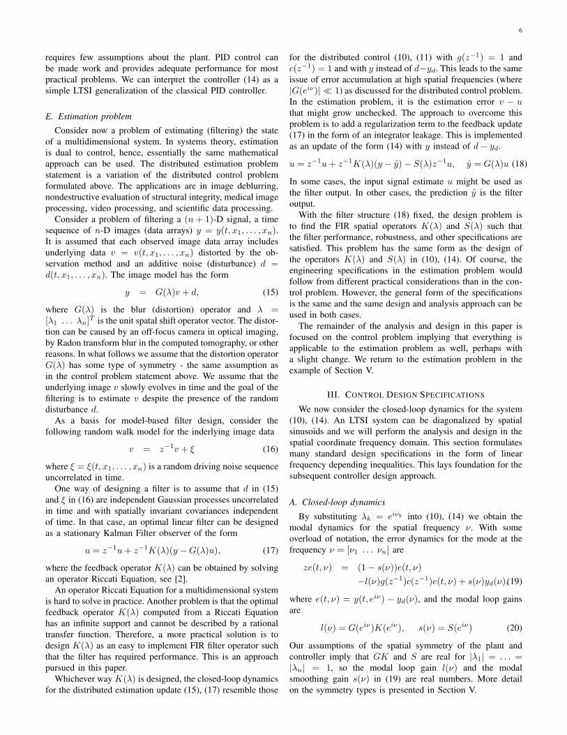
Whichever way K(λ) is designed, the closed-loop dynamicsfor the distributed estimation update (15), (17) resemble those

for the distributed control (10), (11) with g(z−1) = 1 andc(z−1) = 1 and with y instead of d−yd. This leads to the sameissue of error accumulation at high spatial frequencies (where|G(eiν)| ¿ 1) as discussed for the distributed control problem.In the estimation problem, it is the estimation error v − uthat might grow unchecked. The approach to overcome thisproblem is to add a regularization term to the feedback update(17) in the form of an integrator leakage. This is implementedas an update of the form (14) with y instead of d− yd.

u = z−1u + z−1K(λ)(y − y)− S(λ)z−1u, y = G(λ)u (18)

In some cases, the input signal estimate u might be used asthe filter output. In other cases, the prediction y is the filteroutput.

With the filter structure (18) fixed, the design problem isto find the FIR spatial operators K(λ) and S(λ) such thatthe filter performance, robustness, and other specifications aresatisfied. This problem has the same form as the design ofthe operators K(λ) and S(λ) in (10), (14). Of course, theengineering specifications in the estimation problem wouldfollow from different practical considerations than in the con-trol problem. However, the general form of the specificationsis the same and the same design and analysis approach can beused in both cases.

The remainder of the analysis and design in this paper isfocused on the control problem implying that everything isapplicable to the estimation problem as well, perhaps witha slight change. We return to the estimation problem in theexample of Section V.

III. CONTROL DESIGN SPECIFICATIONS

We now consider the closed-loop dynamics for the system(10), (14). An LTSI system can be diagonalized by spatialsinusoids and we will perform the analysis and design in thespatial coordinate frequency domain. This section formulatesmany standard design specifications in the form of linearfrequency depending inequalities. This lays foundation for thesubsequent controller design approach.

A. Closed-loop dynamics

By substituting λk = eiνk into (10), (14) we obtain themodal dynamics for the spatial frequency ν. With someoverload of notation, the error dynamics for the mode at thefrequency ν = [ν1 . . . νn] are

ze(t, ν) = (1− s(ν))e(t, ν)−l(ν)g(z−1)c(z−1)e(t, ν) + s(ν)yd(ν),(19)

where e(t, ν) = y(t, eiν) − yd(ν), and the modal loop gainsare

l(ν) = G(eiν)K(eiν), s(ν) = S(eiν) (20)

Our assumptions of the spatial symmetry of the plant andcontroller imply that GK and S are real for |λ1| = . . . =|λn| = 1, so the modal loop gain l(ν) and the modalsmoothing gain s(ν) in (19) are real numbers. More detailon the symmetry types is presented in Section V.

7

The equation (19) gives another interpretation of our basiccontroller structure: it can be considered as a family ofindependent PID (or other simple structure) controllers, onefor each spatial frequency. The modal loop gain l(ν) and themodal smoothing gain s(ν) are determined by the coefficientsof the spatial filters K and S. The tuning of these filters can beinterpreted as the problem of tuning a family of the controllers,indexed by the spatial frequency vector ν.

Assume first that s(ν) = 0. The modal error e will convergeto zero provided that the loop gain l > 0 is sufficiently smalland the steady-state gain of dynamical controller is such thatg(1)c(1) > 0. The steady-state error in e is eliminated becauseof the integrator (a pole at z=1) present in the controller(14) for S = 0. The modal convergence can be made fasterby increasing the loop gain l within certain limits. This isa usual loopshaping arrangement. The details of tuning theintegrator gain, depend on the plant transfer function g(z−1)and controller transfer function c(z−1).

The operator S (and the gain s(ν)) has an effect of regular-izing the ill-defined problem of controlling a distributed plantwith some zero modal gains. It can be called a ‘smoothing’operator because small gain is usually associated with highspatial frequencies and the regularization has an effect ofreducing the large amplitude of high frequency componentsin the control signal u.

For given plant response dynamics g(z−1) and the dynami-cal controller c(z−1), the closed-loop dynamics (19) are fullydescribed by the two real gains l and s in (20). For given l,s, the dynamics do not depend on the plant spatial operatorG(λ).

Consider now a suitable loop performance index Jp =Jp(l, s). One such simple index can be given by the closedloop convergence rate

Jp(l, s) = maxk|zk|, (21)

where zk are the system poles - the roots of the characteristicequation for (19)

1− z−1 + lz−1g(z−1)c(z−1) + sz−1 = 0.

The performance specification for the controller design canbe expressed in the form

{l, s} ∈ Dp(α), Dp(α) ≡ {l, s : Jp(l, s) ≤ α} (22)

The performance index (21) can be computed numericallyon a two-dimensional grid of the gains {l, s}. From that, usingstandard software, one can obtain the contour lines describingthe boundary of the domain Dp(α). Thus, the specification{l, s} ∈ Dp(α) can be incorporated into the controller designframework.

In what follows, we use a convex approximation of thedomain Dp(α) by inscribing convex polygons inside thisdomains and expressing the domain as the linear inequalitiesof the form

αpl + βps ≤ γp (23)

where αp, βp, γp ∈ <Np express the polygon approxi-mating Dp(α). The inequalities (23), should be interpretedcomponent-wise.

There can be several performance requirements of the form(22), such as feedback loop convergence, limited peaking ofthe loop response, rejection of dynamic disturbances, etc. Therequirements can be also separately formulated for in-band andout-of-band spatial frequencies. The acceptable performancedomain for each requirement can be similarly approximated byan inscribed polygon of the form (23). Combining the linearinequality sets of the form (23) for each of the requirementswould yield a larger set of linear inequalities that still hasthe form (23) and is compatible with the design approachdescribed below.

The domain Dp(α) and its approximation (23) depend onthe plant dynamics g(z−1) = 1, controller c(z−1) = 1 and thespecific chosen performance index. To illustrate validity of thepolygonal approximation of the domain Dp(α) consider twocommonly encountered examples of the dynamics.

Example 1: Simple delay feedback: Assume that g(z−1) =1 and c(z−1) = 1. Such simple response with no dynamicsis encountered in estimation problem and many practicaldistributed control problems where sampling time is muchlarger than the plant settling time. For this system, the singleclosed loop pole is real and the performance index (21) isJp(l, s) = |1 − l − s|. In that case the domain (22) isDp(α) ≡ {l, s : |1− l − s| ≤ α}. It can be exactly expressedin the form (23), where

αp =[ −1

1

], βp =

[ −11

], γp =

[α− 1α + 1

], (24)

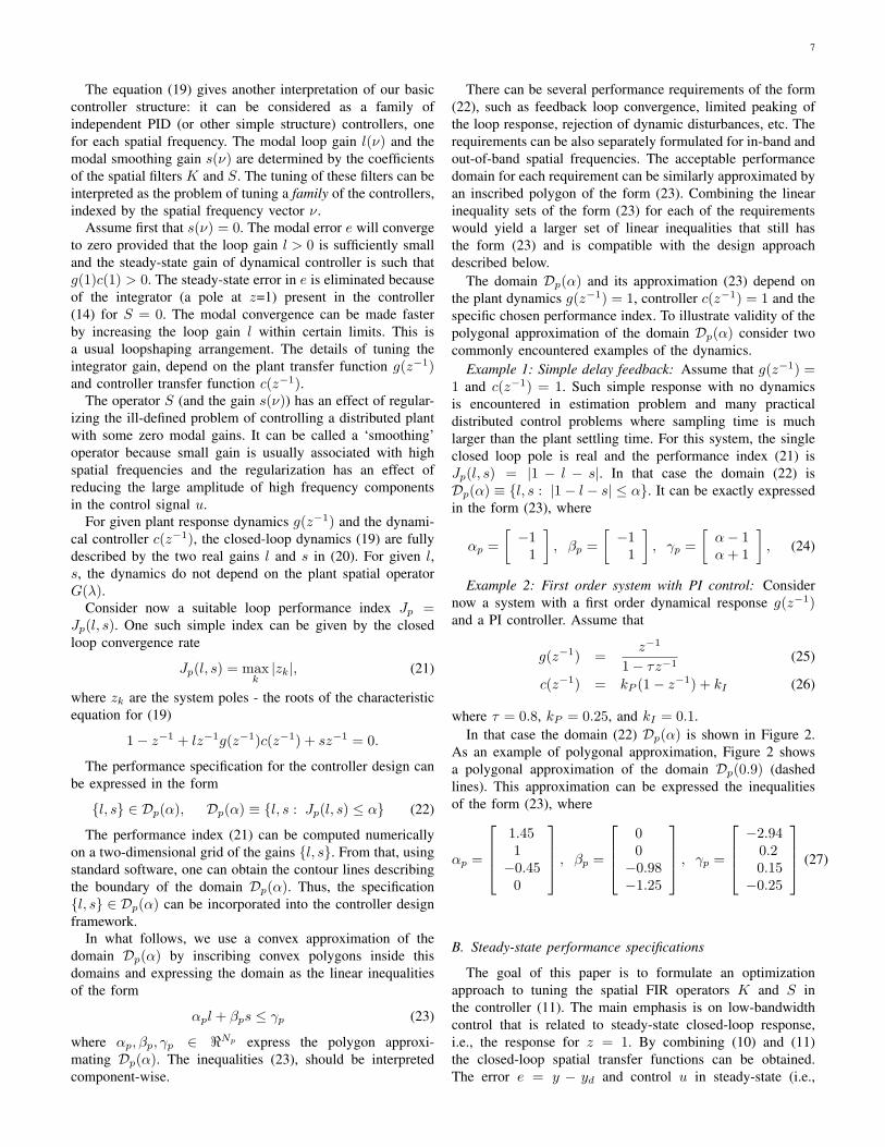
Example 2: First order system with PI control: Considernow a system with a first order dynamical response g(z−1)and a PI controller. Assume that

g(z−1) =z−1

1− τz−1(25)

c(z−1) = kP (1− z−1) + kI (26)

where τ = 0.8, kP = 0.25, and kI = 0.1.In that case the domain (22) Dp(α) is shown in Figure 2.

As an example of polygonal approximation, Figure 2 showsa polygonal approximation of the domain Dp(0.9) (dashedlines). This approximation can be expressed the inequalitiesof the form (23), where

αp =

1.451−0.45

0

, βp =

00−0.98−1.25

, γp =

−2.940.20.15

−0.25

(27)

B. Steady-state performance specifications

The goal of this paper is to formulate an optimizationapproach to tuning the spatial FIR operators K and S inthe controller (11). The main emphasis is on low-bandwidthcontrol that is related to steady-state closed-loop response,i.e., the response for z = 1. By combining (10) and (11)the closed-loop spatial transfer functions can be obtained.The error e = y − yd and control u in steady-state (i.e.,

8

−0.5 0 0.5 1 1.5 2 2.5

−0.2

0

0.2

0.4

0.6

0.8

1

1.2

LOOP GAIN

SM

OO

TH

ING

GA

INDECAY EXPONENT

0.7

0.7

0.7

0.75

0.75

0.75

0.75

0.75

0.80.8

0.8

0.8

0.8

0.8

0.9

0.9

0.9

0.9

0.9

Fig. 2. Performance domain for PID control of a first-order system: thedecay rate index.

at z = 1), and at spatial frequency ν = [ν1 . . . νn]T

(λ = eiν = [eiν1 . . . eiνn ]T ), are given by

e =S(eiν)

S(eiν) + G(eiν)kIK(eiν)yd(ν), (28)

u =kIK(eiν)

S(eiν) + G(eiν)kIK(eiν)yd(ν), (29)

where the integrator gain is kI = c(1). Recall that g(1) = 1is assumed.

For deriving engineering specifications on the control it willbe assumed that a bound on the target profile yd is availablein the form |yd(ν)| ≤ d0, i.e., we have a known bound on themaximum of the of the target profile at every frequency. Werequire that for any such target profile, the magnitude of thecontrol is bounded for all spatial frequencies, i.e., |u| ≤ u0)for all ν ∈ [0, 2π]n. Using (29), the last condition can beexpressed in the form

∣∣∣∣kIK(eiν)

S(eiν) + G(eiν)kIK(eiν)

∣∣∣∣ ≤ u0/d0, for all ν. (30)

In a similar way we require that the magnitude of the steady-state error is bounded, i.e., |e| ≤ e0 for all ν in the bandof spatial frequencies B ⊆ [0, π]n over which we requiregood control performance. This leads to the steady-state per-formance condition∣∣∣∣

S(eiν)S(eiν) + G(eiν)kIK(eiν)

∣∣∣∣ ≤ e0/d0, for all ν ∈ B. (31)

Unlike (30), which is required to hold for any spatial frequencyν, the small steady-state error condition (31) is required onlywithin the spatial bandwidth of the system, ν ∈ B. Thisbandwidth might be taken, for example, as the set of the spatialfrequencies where the plant gain is sufficiently large to ensurethat the disturbances can be compensated without an excessivecontrol effort, i.e.,

{ν ∈ B : |K(eiν)| ≥ k0

}.

Since the bandwidth needs to be defined before the feed-back operator K can be found, a more practical definitioncan be based on the knowledge that kIK(eiν)G(eiν) ≈ 1

in-band. Thus, the bandwidth domain can be defined as{ν ∈ B : |G(eiν)| ≤ g0

}, where g0 = (kIk0)−1.

C. Steady-state robustness specifications

Another important engineering requirement is the robustnessof the closed-loop system to plant modeling error. Assume thatinstead of the plant description (10), we have the followingperturbed plant,

y = g(z−1)G(λ)u + δP (z−1, λ)u, (32)

where |δP | ≤ δ0 for |z| ≤ 1, |λ1| = . . . = |λn| = 1.The small gain theorem guarantees stability of the closed-loop system with perturbed plant (32), and the controller (11),provided∣∣∣∣

c(z−1)K(λ)1− z−1 + z−1S(λ) + z−1c(z−1)g(z−1)G(λ)K(λ)

∣∣∣∣ δ0

< 1 for |z| = 1, |λ1| = . . . = |λn| = 1. (33)

Since in low-bandwidth control the main control action takesplace at low dynamical frequencies, a steady-state robustnesscondition will be considered in place of (33). For |z| = 1, (33)reduces to∣∣∣∣

kIK(λ)S(λ) + kIG(λ)K(λ)

∣∣∣∣ δ0 < 1 for |λ1| = . . . = |λn| = 1. (34)

We can also consider robustness to controller variations. Adistributed controller implementation might differ from thedesigned controller, for several reasons: our analysis does nottake boundary effects into account; and we may have sensor,actuator, or computing element faults in the distributed controlsystem. Assume that instead of the nominal controller (11), wehave

u = z−1u− c(z−1)K(λ)(y − yd)− z−1S(λ)u+ δC(z−1, λ)u, (35)

where |δC| ≤ δC for |z| ≤ 1, |λ1| = . . . = |λn| = 1.Similar to how (34) is derived, the small-gain based steady-state robustness condition can be expressed in the form∣∣∣∣

S(λ)S(λ) + kIG(λ)K(λ)

∣∣∣∣ δC < 1 for |λ1| = . . . = |λn| = 1. (36)

Note that the robustness conditions (34), (36) are homoge-neous in the operators S and K. There is a need to includeone more, nonhomogeneous condition. The integrator in thecontroller might be implemented with an error because of theboundaries and potential faults as mentioned above. A verysmall error in the integrator might results in an instability ifK = 0 and S = 0. This possibility is not covered by thehomogeneous robustness condition (36).

Consider robustness to variations in the smoothing op-erator S. Assume that in (11) the smoothing operator isS(λ) + δS(z−1, λ), where |δS(z−1, λ)| ≤ δS for |z| ≤ 1,|λ1| = . . . = |λn| = 1. Once again, we can derive a small-gain based robustness condition:∣∣∣∣

1S(λ) + kIG(λ)K(λ)

∣∣∣∣ δS < 1 for |λ1| = . . . = |λn| = 1. (37)

9

D. Spatial response decay

Consider now the design requirement related to the bound-ary condition influence. It can be demonstrated that thisinfluence is limited by the characteristic width of the systemimpulse response. The emphasis of other design requirementsconsidered above is on the steady-state closed-loop behavior.Similar to that, we consider the characteristic width of thesteady-state closed-loop impulse response.

The impulse response is defined by a multivariable transferfunction of the form (9) and has the same form as therespective transfer function. The previous subsections considerseveral steady-state transfer functions. For all of these, a steadystate impulse response is described as

h(λ) =A(λ)B(λ)

, B(λ) = S(λ) + kIG(λ)K(λ), (38)

where the denominator is same for all the steady-state looptransfer functions. The numerator A(λ) depends on whichimpulse response is considered. For control response to dis-turbance, A(λ) = kIK(λ), while for the error response todisturbance, A(λ) = S(λ). In the rest of this section, weassume that B(λ) is a FIR operator. The feedback operatorsS(λ) and K(λ) are FIR. The plant spatial response G(λ) canbe modeled or approximated as FIR in most practical cases.We assume that NB is the width of the FIR operator B(λ),such that each of the n indexes of a nonzero element in B(λ)does not exceed NB .

Herein we will evaluate the impulse response width throughits decay rate. The requirement is that the impulse responsedecays at least as fast as r|k|, where k is the distance from theimpulse and r is a design parameter, 0 < r < 1. This responsedecay ensures that boundary condition influence is limited toa boundary layer with a characteristic width

Lb = NA − 1/ log r (39)

where NA is the width of the FIR operator A(λ). An impulseresponse having a decay exponent r requires that the transferfunction A(λ)/B(λ) is analytical in the n-D annulus domain

λ = [λ1 . . . λn]T , r ≤ |λk| ≤ r−1, r < 1, (40)

Technical background on 2-sided z-transform leading to(40) can be found in [27]. The transfer function analyticitymeans that B(λ) should not have zeros in the ring (40).Unfortunately this is a nonconvex constraint and it cannot behandled in a computationally efficient way. Instead, considera convex constraint that conveniently enforces the spatialconveregence and will be further shown to be a relaxationof B(λ) not having zeros in the ring (40). This constraint hasthe form

|1−B(eiν)| ≤ t < 1 (41)

Recall that according to the made symmetry assumptions thefrequency response B(eiν) = S(eiv)+kIG(eiv)K(eiv) is real(or purely imaginary). The condition B(eiν) > 0 is necessaryfor the input-output stability of the transfer function; otherwisethe harmonics with frequency v where B(eiν) = 0 will havean infinite amplification gain. This condition is discussed in

[27] for one spatial variable. Assume now that t = 0. ThenB(λ) ≡ 1 and we got an FIR filter with the transfer functionA(λ). The impulse response of the FIR filter is identicallyzero outside of the FIR filter support.

Consider a general case of 0 < t < 1. One can show thatsmaller t in (41) guarantees faster decay of the filter impulseresponse. The following proposition holds

Proposition 1: Consider an IIR n-D filter A(λ)B(λ) (38), where

a NB-tap delay symmetric denominator B(λ) satisfies (41).Then the impulse response h(k1, . . . , kn) of the IIR filterdecays as

|h(k1, . . . , kn)| ≤ c · rmin[|k1|, ...,|kn|], r = t1/NB , (42)

where c is a constant; r = t1/NB < 1 is the same as in(40); and the boundary layer width estimate (39) is Lb =NA −NB/ log t.

Proof: It is sufficient to prove (42) for the filter 1/B(λ),since a cascade FIR filter A(λ) does not change the responsedecay rate. We will prove the following inequality equivalentto (42)

|h(k1, . . . , kn)| ≤ t−n

1− t, for max[|k1|, . . . , |kn|] ≥ n ·NB (43)

Denote C(λ) = 1−B(λ). For any n > 1

1B(λ)

≡ 11− C(λ)

=[1 + C(λ) + . . . + Cn−1(λ)

]+

Cn(λ)1− C(λ)

(44)

The first n terms in the square brackets in the r.h.s. (44)describe an FIR filter with the width (n−1)NB . The impulseresponse of this FIR filter is zero for max[|k1|, . . . , |kn|] ≥n · NB . For max[|k1|, . . . , |kn|] ≥ n · NB , using theinverse Fourier transform to evaluate the impulse responseh(k1, . . . , kn) yields

h(k1, . . . , kn) =

1(2π)n

∫ 2π

0

...

∫ 2π

0︸ ︷︷ ︸n

1B(eiν)

e−ik1ν1 · · ·e−iknνndν1· · ·dνn

=1

(2π)n

∫ 2π

0

...

∫ 2π

0︸ ︷︷ ︸n

Cn(eiν)1− C(eiν)

e−ikT νdν (45)

In accordance with (41), |C(eiν)| ≤ t < 1. Hence,∣∣∣ Cn(eiν)1−C(eiν)

∣∣∣ ≤ tn

1−t and (43) follows immediately. Q.E.D.

E. Specification summary

In summary, the specifications are given by the loop-gainlimit for dynamic stability (14), and• the actuator limit (30)• the performance specification (31)• robustness to plant variation (34)• robustness to controller variation (36)• robustness to smoothing operator variation (37).• performance specifications (23)• spatial decay specifications (41)

10

Since the loop gain l(ν) is a linear function of K(ν) and thesmoothing gain s(ν) is a linear function of S(ν) the feedbackgain constraints (23), are linear in K and S for each frequencyν. Each of the other specifications has the form of a limit onthe magnitude of a linear fractional function of K(λ) andS(λ), for all |λ1| = . . . = |λn| = 1, or (in the case of theperformance specification) for some |λ1| = . . . = |λn| = 1.

IV. OPTIMIZATION FORMULATION

We now show how the design of the spatial filters Kand S can be cast as a semi-infinite convex optimizationproblem, which can be approximated well as a linear program(and therefore solved efficiently). As briefly mentioned inSection III, these operators are constrained to be FIR operatorssuch that information from near neighbors only is used whencomputing control at a particular spatial location. See [6]for a discussion of advantages to the convex optimizationformulation.

A. Symmetry and realness

Recall that we assume that the plant spatial response oper-ator G(λ) is symmetric, such that G(eiν) is real. We assumethat the feedback operators K(λ) and S(λ) are symmetric too.Alternatively, the approach described below is applicable whenG(λ) is symmetric for some coordinates and anti-symmetricfor other. In that case we assume that K(λ) pocesses the samesymmetry such that the frequency response K(eiν)G(eiν) isreal.

To provide a deeper insight into the operator symmetry anda background for the technical approach formulation, let usconsider several types of symmetry.

1-D case: Let us start from the case of one spatial variable,when λ is a scalar. In the case when the FIR operator K issymmetric (which we assume when G is symmetric), we canexpress it as

K(λ) = κ0 +N∑

k=1

(λk + λ−k)κk, (46)

where κ0, . . . , κN are the coefficients. When G(λ) is anti-symmetric, we take K to be anti-symmetric as well, in whichcase it has the form

K(λ) =N∑

k=1

(λk − λ−k)κk. (47)

(We will explain the method assuming that K and G aresymmetric.) The smoothing FIR operator S(λ) is alwaysassumed to be symmetric, and has the form

S(λ) = σ0 +N∑

k=1

(λk + λ−k)σk, (48)

where σ0, . . . .σN are the coefficients. At the spatial frequencyν, i.e., λ = eiν , we have

K = κ0 + 2N∑

k=1

κk cos(kν), S = σ0 + 2N∑

k=1

σk cos(kν). (49)

Let x ∈ R2N+2 be the vector of all the coefficients, i.e., ouroptimization variables:

x = [κ0 · · · κN σ0 · · · σN ]T . (50)

For each spatial frequency ν, K and S are linear functionsof x, and therefore so are the loop and smoothing gains, l(ν)and s(ν).

2-D symmetries: Let us discuss the symmetry patterns fora 2-D operator

B(λ) = B(λ1, λ2) =M∑

m=1

M∑n=1

bm,nλm1 λn

2

This operator could correspond to either of the two FIRfeedback operators K(λ) or S(λ). The types of symmetryusually considered for 2-D filters include (see [25])• 2-fold symmetry: bm,n = b−m,−n

• 4-fold symmetry: bm,n = b−m,−n = b−m,n = bm,−n

• 8-fold symmetry: bm,n = b−m,−n = b−m,n = bm,−n =bn,m = b−n,−m = b−n,m = bn,−m

In all of the above symmetry cases the operator B(λ) canbe expanded in the form similar to (46)–(48)

B(λ1, λ2) =Mb∑

m=0

bmPMm (λ1, λ2), (51)

where PMm (λ1, λ2) are the elementary polynomials defining

the symmetry. The expansion (51) explicitly shows Mb + 1independent filter design parameters bm for the assumedsymmetry type.

For 2-fold symmetry, the symmetric expansion polynomialscan be expressed in the form

PM0 (λ1, λ2) = 1,

PMj (λ1, λ2) = λj

2 + λ−j2 , (j = 1, . . . , M),

PMM+k(λ1, λ2) = λlk

1 λmk2 + λ−lk

1 λ−mk2 , (52)

where in the last line 1 ≤ lk ≤ M , −M ≤ mk ≤ M andk = 1, . . . ,M(2M + 1). The expansion size is Mb = 1 +M + M(2M + 1).

For 4-fold symmetry

λPM0 (λ1, λ2) = 1,

PMj (λ1, λ2) = λj

1 + λ−j1 + λj

2 + λ−j2 , (j = 1, . . . , M),

PMM+k(λ1, λ2) = λlk

1 λmk2 + λlk

1 λ−mk2

+ λ−lk1 λmk

2 + λ−mk1 λ−lk

2 , (53)

where in the last line 1 ≤ lk ≤ M , 1 ≤ mk ≤ M , andk = 1, . . . ,M2. The expansion size is Mb +1 = 1+M +M2.

For 8-fold symmetry

PM0 (λ1, λ2) = 1,

PMj (λ1, λ2) = λj

1 + λ−j1 + λj

2 + λ−j2 ,

PMM+j(λ1, λ2) = λj

1λj2 + λ−j

1 λj2

+ λj1λ−j2 + λ−j

1 λ−j2 ,

PM2M+k(λ1, λ2) = λlk

1 λmk2 + λlk

1 λ−mk2 + λ−lk

1 λmk2

+λ−lk1 λ−mk

2 + λmk1 λlk

2 + λmk1 λ−lk

2

+λ−mk1 λlk

2 + λ−mk1 λ−lk

2 , (54)

11

where j = 1, . . . ,M ; in the last equation 1 ≤ lk ≤ mk − 1,2 ≤ mk ≤ M , and k = 1, . . . ,M(M − 1)/2. The expansionsize is Mb + 1 = 1 + 2M + M(M − 1)/2.

Choosing a higher type of symmetry reduces the number offilter design parameters and is desirable where the symmetryof the requirements exists. To obtain frequency responses in(51)–(54), substitute λ1 = eiv1 and λ2 = eiv2 . Because of thesymmetry, the imaginary parts cancel and the real expansionfunctions PM

m (eiw1 , eiw2) are combinations of the frequencycosines.

In all of the considered symmetry cases, the frequencyresponses for the FIR feedback operators K and S in thecontroller (11) can be expressed in the same general form

K(eiν1 , eiν2) = cTK(eiν1 , eiν2)pK ,

S(eiν1 , eiν2) = cTS (eiν1 , eiν2)pS , (55)

cK(eiν1 , eiν2) = [PM0 (eiν1 , eiν2) . . . PM

Mb(eiν1 , eiν2)]T ,

pK = [κ0 κ1 . . . κMb]T , (56)

cS(eiν1 , eiν2) = [PM0 (eiν1 , eiν2) . . . PM

Mb(eiν1 , eiν2)]T ,

pS = [σ0 σ1 . . . σMb]T , (57)

Let x ∈ R2Mb+2 be the vector of all the coefficients, i.e.,our optimization variables:

x = [κ0 · · · κN σ0 · · · σN ]T . (58)

For each spatial frequency ν, K and S are linear functionsof x, and therefore so are the loop and smoothing gains, l(ν)and s(ν).

Other symmetries: One additional type of symmetry for2-D array is hexagonal symmetry. Hexagonal actuator arraysare commonly used in adaptive optics where several thousandactuators might be used to control surface of a deformablemirror. A distributed control application with a hexagonalsymmetry is considered in [31].

Some 3-D and 4-D applications of distributed feedbackcontrol exist on the estimation side, such as computationaltomography or time-space filtering. A discussion of the filtersymmetry types for such systems can be found in [29], [9].

The design and implementation approaches presented hereinare directly applicable to higher-dimensional IIR filters. Theonly difference in the formulation is in the number of theindependent coordinate arguments. The only difference in thecomputational design and implementation methods is in thepotentially larger number of the points in a multidimensionalfrequency grid.

One more extension of the presented approach is to the casewhere G(λ) is not symmetric. In that case the system can be‘squared down’ by multiplying the plant output y in (10) by theconjugated operator G∗(λ). This yields the system of the sameform (10) with a symmetric spatial response G∗(λ)G(λ). The‘squaring down’ is especially efficient if G is a FIR operator.

B. Optimization problem

We will now show how all of the tuning specifications canbe expressed as (infinite) sets of linear inequalities on thevariable x (58). The operators K, and S, as well as the loop

gain GK are linear in the tuning weights (components of thevector x. Therefore the following representation is possible

K(eiν) = K(ν)T x, S(eiν) = S(ν)T x,

kIG(eiν)K(eiν) = H(ν)T x, (59)

where K(ν), S(ν), and H(ν) are column vectors with realcomponents.

Expressing the constraints which involve linear fractionalfunctions as linear constraints is not as straightforward. Foreach spatial frequency ν, the requirements (30), (31), (34),(36), and (37) have the form∣∣∣∣

aT x + b

s(ν) + kI l(ν)

∣∣∣∣ ≤ 1, (60)

where a ∈ R2Mb+2 and b ∈ R (and depend on the spatialfrequencies, and also which specification is being represented).

Both the numerator and denominator in this equality aretransformation of the operators K and S, which are in turnlinear in the tuning parameters κk and σl in (46), (47), (48).In all cases the denominator is

S(eiν) + kIG(eiν)K(eiν) (61)

The second term in the denominator, kI l(ν), is nonnegative,and is positive except at spatial frequencies where the plantgain is zero. In fact, the whole denominator must be positive atall spatial frequencies; indeed, the whole point of the smooth-ing operator S is to ensure s(ν) > 0 for spatial frequencieswhere l(ν) is small. We can argue this as follows. Supposethe denominator (which is real) changes sign, and thereforeis zero at some spatial frequency ν. At that frequency, therobustness to smoothing operator variation constraint, (37), isviolated, since the numerator of the relevant transfer functionis a nonzero constant, and the denominator vanishes, so therelevant transfer function is infinite (and certainly not less thanone in magnitude). Thus, we have

s(ν) + kI l(ν) > 0 for all ν, (62)

for any controller that satisfies all the specifications. Since thedenominator is positive, we can multiply through by it, andexpress the linear fractional constraint (60) as

−(s(ν) + kI l(ν)) ≤ aT x + b ≤ s(ν) + kI l(ν). (63)

This is a pair of linear inequalities in the variable x, sinceboth s(ν) and l(ν) are linear functions of x.

With the notation (59) and taking into account (50), the con-troller design specifications for steady-state loop performance(31), (30), (34), (36), (37) can be presented in the form

−S(ν)T x− H(ν)T x ≤ (d0/u0)K(ν)T x

≤ S(ν)T x + H(ν)T x (64)−S(ν)T x− H(ν)T x ≤ (d0/e0)S(ν)T x

≤ S(ν)T x + H(ν)T x (65)−S(ν)T x− H(ν)T x ≤ δ0K(ν)T x

≤ S(ν)T x + H(ν)T x (66)−S(ν)T x− H(ν)T x ≤ δC S(ν)T x

≤ S(ν)T x + H(ν)T x (67)−S(ν)T x− H(ν)T x ≤ δS ≤ S(ν)T x + H(ν)T x (68)

12

where (65) is required to hold only within the assumed spatialbandwidth of the control, i.e., for ν ∈ B.

These specifications should be complemented by the loopdynamical response specifications (23) that can be presentedin the form

αpH(ν)T x + βpS(ν)T x + γp ≤ 0 (69)αoH(ν)T x + βoS(ν)T x + γo ≤ 0 (70)

where (69) is required to hold only in the control band, i.e.,for ν ∈ B, and (70) is required to hold only out-of-band, forν /∈ B.

Finally, as the optimization objective we consider the spatialresponse decay. We require that the transfer function de-nominator B(eiν) = s(ν) + kI l(ν) satisfies (41), where wewill minimize t. In accordance with Proposition 1 the decayrate bound is guaranteed to improve for smaller t. Roughlyspeaking, we want the (dynamic) loop gain as uniform aspossible for all spatial frequencies. We can achieve this goalby taking as objective

φ(x) = maxν∈[0,2π]n

|1− S(ν)T x− H(ν)T x|. (71)

Since this objective is the maximum of a family of convexfunctions (absolute values of linear functions), it is a convexfunction of x. If φ is small, then we can expect fast spatialdecay of the closed-loop system response.

The overall design problem is a convex optimization prob-lem:

minimize φ(x)subject to linear inequalities (63) above, for each ν.

The objective is given in (71), and the constraints are aninfinite set of linear inequalities; specifically, ten per spatialfrequency ν. (Such a problem is called semi-infinite since theconstraints are indexed by the real number ν.)

Finally, we approximate the semi-infinite convex problemas an LP. We take a finite but sufficiently dense set ofspatial frequencies, {ν1, . . . , νM}, and impose all of the linearinequalities at these frequencies only. This results in a large,but finite, number of linear inequalities. In practice, the numberM of the frequency gridpoints required would depend on thehighest spatial frequency in the representation (49) or (59) ofthe spatial operators (the largest tap delay in the FIR operatorsS and K). Of course, the frequency content of the systemspatial operator G(eiν) also needs to be taken into account.Refining the frequency grid always allows to achieve anyprescribed accuracy of the solution.

Similarly, we approximate the objective by sampling overspatial frequencies:

φ(x) = maxνi

|1− S(νi)T x− H(νi)T x|.

This is a piecewise linear and convex function of x. We canin turn formulate this sampled problem as a linear program,by introducing a new variable γ, and adding the constraints

−γ ≤ 1− S(νi)T x− H(νi)T x ≤ γ, (72)

These constraints ensure that γ ≥ φ(x). Then we formulatethe following linear program:

minimize γsubject to −γ ≤ 1− S(νi)T x− H(νi)T x ≤ γ,

linear inequalities (63) for each νi.(73)

In this problem, the objective and all constraints are linear,i.e., it is a linear program (LP).

The LP (73) has 2Mb +3 variables, and no more than 18Mlinear inequality constraints. (The exact number depends onthe number of spatial frequency samples that fall in the controlband B.) It can be solved very quickly for typical problemsizes, e.g., several tens of variables, and several hundreds ofconstraints.

This method of synthesizing the spatial filters K and S canbe used to tune the LTSI controller, by varying parameters inthe specifications, such as the control band B, the actuator limitu0, the error limit e0, and the constants related to various typesof uncertainty, i.e., δ0, δC , and δS . These parameters becomethe ‘knobs’ used by the control designer, that are varied toobtain adequate performance.

It should be clear from the discussion that many otherspecifications can also be included, and more complex speci-fications can also be handled by the method. As an example,we can impose a limit on loop gain that is a function of spatialfrequency. In addition, we can impose limits on the magnitudeof any steady-state closed-loop spatial transfer function, sinceevery one will be linear fractional, with the same denominatoras the ones considered.

V. SIMULATION EXAMPLE

As an example of applying the proposed feedback designapproach, we consider a 3-D distributed estimation problemfor a 2-D image evolving in time. The motivation for the prob-lem below comes from estimating a slowly changing imagefrom a series of noisy snapshots. Such images are common inindustrial vision systems, medical diagnostics, nondestructiveevaluation of materials. A closely related problem is of imagedeblurring.

2 4 6 8 10 12

24

68

1012

0.01

0.02

0.03

SPATIAL IMPULSE RESPONSE − PSF OF BLUR OPERATOR

Fig. 3. Spatial response (point spread function) of the image bluroperator

We assume a model of the form (15) where the 2-D FIRoperator G(λ) describes a Point Spread Function (PSF) of theimaging system. In practice, the PSF could be often deter-mined by applying a point signal in a controlled experimentand observing the imaging system response. In this simulation

13

example we postulate that G(λ) is a known Gaussian bluroperator

G(λ) =NG∑

n=−NG

NG∑

k=−NG

e−12 (n2+k2)/a2

Gλn1λk

2 , (74)

where the Gaussian width aG = 2 and maximal delay of FIRoperator NG = 6 were assumed. The blur PSF operator G(λ)is illustrated in Figure 3.

For the estimator design it was assumed that the dynamicsare absent except the processing delay and a simple integralfeedback of the form (11) is used such that

g(z−1) = 1, c(z−1) = 1 (75)

The plant spatial operator G(λ) in (74) has an 8-foldsymmetry. Therefore the operators K and S in the controller(11) are also chosen to be 8-fold symmetric. These operatorsare represented in the form (55)–(57), (54) to yield

K(eiν1 , eiν2) = K(ν1, ν2)T x, S(eiν1 , eiν2) = S(ν1, ν2)T x,

kIG(eiν1 , eiν2)K(eiν1 , eiν2) = H(ν1, ν2)T x, (76)

where K, S, and H follow from (54), (56), (57).Both operators K and S have M = 5 FIR taps on each side

off the center, thus, with the 8-fold symmetry there are a totalof Mb + 1 = 1 + 2M + M(M − 1)/2 = 21 coefficients ineach of the two FIR operators to be optimized.

The specifications for the estimator filter are formulatedseparately in the bandwidth domain (pass band) Bp and stopband Bs. These domains were selected as

Bp = {ν1, ν2 : |G(eiν1 , eiν2)| ≥ 0.25},Bs = {ν1, ν2 : |G(eiν1 , eiν2)| ≤ 0.1} (77)

We consider the following specifications for the estimatordesign.

Convergence (dynamical performance): For the estimatordesign, the specifications (22) have the form similar to (23).In-band (in the pass band), the estimate is required to convergequickly enough such that the filtered signal responds quicklyto the change of the underlying image. On the opposite,dynamical low-pass filtering in the (spatial) stop band isrequired to be heavy enough. The filter time constant shouldbe no less than a given value such that the dynamical noise issufficiently reduced. These requirements can be expressed as

∣∣1− H(ν1, ν2)T x− S(ν1, ν2)T x∣∣ ≤ αp, ν ∈ Bp, (78)

αs ≤ 1− H(ν1, ν2)T x− S(ν1, ν2)T x ≤ 1, ν ∈ Bs, (79)

where αp = 0.7 and αs = 0.85 were assumed in the designexample. This corresponds to the filter time constant being nomore than 2.8 samples in band and no less than 6 samples inthe stop band.

Steady-state Performance: The steady-state filter outputcan be expressed from (15), (18) as (kI = c(1) = 1)

u =K(eiν1 , eiν2)

S(eiν1 , eiν2) + K(eiν1 , eiν2)G(eiν1 , eiν2)y,

y = G(eiν1 , eiν2)u (80)

The requirements to the steady state performance of theestimator follow from (80). The estimate y should be closeto the signal y in band. This can be expressed as the transferfunction relating y to y being close to unity in the pass band.To reject the noise, the signal y should be small in the stopband. The transfer function magnitude should be small.

Assume a bound v0 on the magnitude of the source imagev and a bound d0 on the magnitude of the disturbance d. Bysubstituting (76) into (80) and making the estimates similar to(34), (36) we obtain the steady state performance requirementsin the form

H(ν1, ν2)T x ≤ (1 + E) · (S(ν1, ν2)T x + H(ν1, ν2)T x),

H(ν1, ν2)T x ≥ (1− E) · (S(ν1, ν2)T x + H(ν1, ν2)T x),

for {ν1, ν2} ∈ Bp (81)∣∣H(ν1, ν2)T x∣∣ ≤ V1 ·

(S(ν1, ν2)T x + H(ν1, ν2)T x

),

for {ν1, ν2} ∈ Bs (82)

0 0.5 1 1.5 2 2.5 3−0.2

0

0.2

0.4

0.6

0.8

1

1.2

FREQUENCY = (v12 + v

22)1/2

MA

GN

ITU

DE

Fig. 4. Filter specification requirements: 1-D cross section of the require-ments in the 2-D domain of spatial frequencies.

In the design example we assumed E = 0.25 and V1 =0.25. The design requirements are illustrated in Figure 4. Theycan be expressed as as linear inequalities in the form similarto (64), (65).

The requirements (81), (82) need to be complemented by therequirement of the bounded amplification of the input signaly when computing the intermediate estimate u in (80). Unlessthis requirement is in place, the large intermediate signal ucould lead to instability caused by the boundary effects.

V0

∣∣K(ν1, ν2)T x∣∣ ≤ S(ν1, ν2)T x + H(ν1, ν2)T x, (83)

where {ν1, ν2} ∈ [0, 2π]2. In the design example, V0 = 3was assumed.

Spatial response decay: Finally, as the optimizationobjective we will take the decay rate of the steady state closed-loop response (boundary layer width). This objective can beexpressed in the following form that is similar to (71) with apotential scaling factor difference.

−1 ≤ γ1 ≤ 1− S(ν1, ν2)T x− H(ν1, ν2)T x ≤ γ2 ≤ 1 (84)γ2 − γ1 → min

A. Estimator implementation and simulation results

The formulated linear inequalities and the optimizationobjective (84) were integrated together to yield an optimiza-tion problem with respect to the parameter vector x =[pT

S pTK q1 q2]T , where pS and pK each contain 21 inde-

pendent coefficients of the respective FIR operators S and

14

K to be optimized, 44 coefficients at all in the parametervector x (58). The controller tuning problem was cast as anLP problem with respect to x, as described above, with spatialfrequency sampled at 64×64 = 4096 points uniformly spacedin the spatial frequency domain [0, 2π]× [0, 2π]. The problemwas solved using the LINPROG medium-scale LP solver fromMatlab R© Optimization Toolbox. The designed spatial FIRoperators K and S of the filter are illustrated in Figure 5.

−5

0

5 −50

5

−0.04

−0.02

0

0.02

0.04

ERROR FEEDBACK OPERATOR

−5

0

5 −50

5

0

0.05

0.1

SMOOTHING OPERATOR

Fig. 5. Designed spatial FIR operator for the 3-D estimator filter. Feedbackoperator K - upper plot, smoothing operator S - lower plot.

Fig. 6. Filter magnitude response function for steady state (w = 0).

The transfer function magnitude for the designed filter atsteady state (at w = 0) is displayed in Figure 6. Figure 7shows the time constant of the filter depending on the spatialfrequency

τ(ν1, ν2) =−1

log (1−K(eiν1 , eiν2)G(eiν1 , eiν2)− S(eiν1 , eiν2)).

The steady-state spatial impulse response of the filter isillustrated in Figure 8. It decays in 5-8 samples off the centers.This shows how far the influence of the boundary conditionswould extend onto the spatial domain of the filtered signal.

The designed filter was applied to a noisy image sequencegenerated as follows. The spatial domain of 40 × 100 pixels

Fig. 7. Filter time constant τ(ν1, ν2) depending on the spatial modefrequencies.

−50

5−5

05

0

0.02

0.04

0.06

FILTER IMPULSE RESPONSE

Fig. 8. Steady state impulse response of the closed loop.

0 5 10 15 20 25 30 35 40 45 50

0

0.2

0.4

0.6

0.8

1

TIME

ME

AN

ES

TIM

AT

E

Fig. 9. Correlation between the applied and estimated signal (solid line).Time series of the applied signal amplitude (dashed line)

Fig. 10. Noisy data snapshot (upper plot). Filtered data snapshot (lower plot)

15

was considered with the source signal v being zero in themost of the domain, except an ellipse with the main axes of8 (along x1) and 20 (along x2) in the center of the domain.The signal v was ramped up from zero to unity in 12 timesteps uniformly inside the ellipse. The signal v was distortedby an additive (pseudo-)random noise uniformly distributed inthe interval [−2, 2] and uncorrelated in time and space. Thenoisy signal was then smoothed (blurred) by applying a scaledBlackman window (a FIR operator [0.2024 0.5952 0.2024])along each of the directions x1 and x2. The generated 3-Dsignal was used as an input to the designed filter. In practicethe blur might be not known accurately, which is reflected bythe blur in the simulation being differs from what is assumedin the filter design. The simulation results are illustrated inFigures 9 and 10.

The time dependency of the filtered data can be illustratedby taking average values inside the central ellipse and outsideof it. The time series for these average values are illustratedin Figure 9. The plot also show the magnitude of the sourcesignal inside the ellipse (it is zero outside). The time seriesfor the filtered signal follows the time dependencies for thesource very closely. This means that despite the significantimprovement in signal-to noise ratio, the filtering delay isinsignificant.

The 2-D slices of the signals in Figure 10 is taken at time50 well afer the end of the ramp. The raw, noisy, 2-D data inthe upper plot makes the source signal v hardly visible. In thefiltered data, (the lower plot) the signal is significantly (factor3-5) above the noise.

VI. CONCLUSIONS

The LP optimization scheme for distributed controller tun-ing has been proposed. A straightforward design approachimplements many engineering specifications in natural frame-work. It was demonstrated through simulation that the pro-posed method allows achieving very good quality of controland estimation in difficult distributed system problems.

REFERENCES

[1] Abraham, R. and Lunze, J. “Modelling and decentralized control of amultizone crystal growth furnace,” Int. J. Robust and Nonlinear Control,Vol.2, 1992, pp. 107–122.

[2] Bamieh, B., Paganini, F., and Dahleh, M. “Distributed control ofspatially-invariant systems,” IEEE Trans. on Automatic. Contr., Vol. 47,No. 7, July 2002. pp. 1091–1107.

[3] Beck, C.L. and Doyle, J. and Glover, K. “Model reduction of multidi-mensional and uncertain systems,” IEEE Trans. on Automatic Control,Vol. 41, No. 10, 1996, pp. 1466–1477.

[4] Bose, N.K. Applied Multidimensional Systems Theory, Van NostrandReynhold, 1982

[5] Boyd, S. and Barratt, C. Linear Controller Design: Limits of Perfor-mance, Prentice-Hall, 1991

[6] Boyd, S. and Vandenberghe, L. Convex Optimization, Cambridge Uni-versity Press, 2004.

[7] Brockett, R.W. and Willems, J.L. “Discretized partial differential equa-tions: examples of control systems defined on modules,” Automatica,Vol. 10, 1974, pp. 507–515.

[8] Chottera, A. and Jullien, G. “Design of two-dimensional recursive digitalfilters using linear programming,” IEEE Trans. on Circuits and Systems,Vol. 29, No. 12, 1982, pp. 817–826.

[9] Coulombe, S. and Dubois, E. “Linear phase and symmetries for mul-tidimensional FIR filters over lattices,” IEEE Trans. Circuits Syst. II,Analog Digit. Signal Process., Vol. 45, Apr. 1998, pp. 473-481.

[10] D’Andrea, R. “Linear matrix inequaly approach to decentralized controlof distributed parameter systems,” American Control Conf., Philadelphia,PA, pp.1350–1354, June 1998

[11] D’Andrea, R., and Dullerud, G.E., “Distributed control for spatiallyinterconnected systems,” IEEE Trans. on Automatic Control, Vol. 48,No. 9, 2003, pp. 1478–1495.

[12] De Castro, G. A. and Paganini, F. “Convex synthesis of localizedcontrollers for spatially invariant systems,” Automatica, Vol. 38, No.3, 2002, p.445-450.

[13] Special Issue on Control of Industrial Spatially Distributed Processes,Eds. Dochain, D., Dumont, G., Gorinevsky, D., and Ogunnaike, T., IEEETrans. on Control Systems Technology, Vol. 11, No. 5, 2003.

[14] Dudgeon, D.E. and Mersereau, R.M. Multidimensional Digital SignalProcessing, Prentice-Hall, 1984.

[15] Duncan, S. R. , “The design of robust cross-directional control systemsfor paper making,” American Control Conf., pp. 1800–1805, Seattle ,WA, 1995.

[16] Gorinevsky, D. “Loop-shaping for iterative control of batch processes,”IEEE Control Systems Magazine, Vol. 22, No. 6, 2002, pp. 55–65.

[17] Gorinevsky, D. and Boyd, S. “Optimization-based design and imple-mentation of multi-dimensional zero-phase IIR filters,” IEEE Trans. onCircuits and Systems - I, Vol. 53, No. 2, 2006, pp. 372-386

[18] Gorinevsky, D., Boyd, S., and Stein, G. “Optimization-based tuningof low-bandwidth control in spatially distributed systems,” AmericanControl Conference, Vol. 3, pp. 2658–2663, Denver, CO, June 2003.

[19] Gorinevsky, D. and Gheorghe, C. “Identification tool for cross-directional processes,” IEEE Trans. on Control Systems Technology, Vol.11, No. 5, 2003, pp. 629–640.

[20] Gorinevsky, D. and Gordon, G. “Spatio-temporal filter for structuralhealth monitoring,” American Control Conf., Minneapolis, MN, June2006

[21] Gorinevsky, D. and Stein, G. “Structured uncertainty analysis of robuststability for multidimensional array systems,” IEEE Trans. on AutomaticControl, Vol. 48, No. 8, 2003, pp. 1557–1568.

[22] Gorinevsky, D., Hyde, T., and Cabuz, C. “Distributed shape control oflightweight space reflector structure,” IEEE Conference on Decision andControl, Vol. 4, pp.3850–3855, Orlando, FL, December 2001,

[23] Heaven, E.M., Jonsson, I.M., Kean, T.M., Manness, M.A., and Vyse,R.N. “Recent advances in cross machine profile control,” IEEE ControlSyst. Mag., vol. 14, no. 5, Oct. 1994.

[24] Langbort, C. and D’Andrea, R. “Distributed control of spatially re-versible interconnected systems with boundary conditions,” SIAM Jour-nal of Control and Optimization, vol. 44, no. 1, 2005, pp. 1–28.

[25] Lim, J.S. Two-Dimensional Signal and Image Processing, Prentice Hall,1990.

[26] Mijanovic, S., Stewart, G.E., Dumont, G.E., and Davies, M.S. “Designof an industrial distributed controller near spatial domain boundaries,”American Control Conference, Vol. 4, pages 3574–3580, Boston, MA,June 30-July 3, 2004.

[27] Oppenheim, A.V., Schafer, R.W., and Buck, J.R. Discrete-Time SignalProcessing, Prentice Hall, 1999 A recursive information flow system fordistributed control arrays

[28] Paganini, F., “A recursive information flow system for distributed controlarrays,” American Control Conf., Vol. 6, pages 3821–3825, San Diego,CA, 2-4 June, 1999.

[29] Pitas, J. and Venetsanopoulos, A. “The use of symmetrics in the designof multidimensional digital filters,” IEEE Trans. on Circuits and Systems,Vol. 33, No. 9, 1986, pp. 863–873.

[30] Rabiner, L., Graham, N., and Helms, H. “Linear programming designof IIR digital filters with arbitrary magnitude function,” IEEE Trans. onAcoustics, Speech, and Signal Processing , Vol. 22, No. 2, 1974, pp.117 - 123.

[31] Stein, G. and Gorinevsky, D. “Design of surface shape control for largetwo-dimensional arrays,” IEEE Trans. on Control Systems Technologyvol. 13, no. 3, pp. 422 - 433, May 2005.

[32] Stewart, G.E., Gorinevsky, D., and Dumont, G.A. “Feedback controllerdesign for a spatially-distributed system: The paper machine problem,”IEEE Trans. on Control Systems Technology, Vol. 11, No. 5, 2003, pp.612–628.

[33] Stewart, G.E., Gorinevsky, D., and Dumont, G.A. “Two-dimensionalloop shaping,” Automatica, Vol. 39, No. 5, 2003, pp. 779-792.

[34] Tikhonov, A.N., and Arsenin, V.Ya. Solutions of Ill-Posed Problems.Halsted Press, Washington, 1977.

[35] Wu, S.-P., Boyd, S., and Vandenberghe, L. “FIR Filter Design via Spec-tral Factorization and Convex Optimization,” Applied and ComputationalControl, Signals and Circuits, Ch. 2, pp. 51–81, Birkhauser, 1997

16

PLACEPHOTOHERE

Dimitry Gorinevsky (M’91–SM’98–F’06) receiveda Ph.D. degree from department of mechanics andmathematics of Moscow (Lomonosov) University, in1986, and a M.Sc. in aerospace engineering fromthe Moscow Institute of Physics and Technology, in1982.

He is a Consulting Professor of Electrical Engi-neering at Stanford University and an independentconsultant to NASA. He worked for Honeywell for10 years. Prior to that, he held research, engineering,and academic positions in Moscow, Russia; Munich,

Germany; Toronto and Vancouver, Canada. His interests are in decisionand control systems applications across many industries. He has authoreda book, more than 140 reviewed technical papers and a dozen patents. Dr.Gorinevsky is an Associate Editor of IEEE Transactions on Control SystemsTechnology. He is a recipient of Control Systems Technology Award, 2002,and Transactions on Control Systems Technology Outstanding Paper Award,2004, of the IEEE Control Systems Society.

PLACEPHOTOHERE

Stephen Boyd (S’82–M’85–SM’97–F’98) receivedthe A.B. degree in Mathematics from Harvard Uni-versity in 1980, and the Ph.D. in Electrical Engi-neering and Computer Science from the Universityof California, Berkeley, in 1985.

He is currently the Samsung Professor of En-gineering, and Professor of Electrical Engineeringin the Information Systems Laboratory at StanfordUniversity. His current research focus is on convexoptimization applications in control, signal process-ing, and circuit design.

PLACEPHOTOHERE

Gunter Stein (S’66–M’69–F’85) received a PhDin Electrical Engineering from Purdue University in1969.

He is a Chief Scientist (ret) of Honeywell Tech-nology Center (now Honeywell Labs). His technicalspecialization is in systems and control, particularlyaircraft flight controls (fighters, transports, and ex-perimental vehicles), spacecraft attitude and orbitcontrols, and navigation systems for strategic, tac-tical, and commercial applications. From 1977 to1997, Dr. Stein also served as Adjunct Professor

in EE and CS at MIT, teaching control systems theory and design. He isalso active in the development of computer aids for control system design.Dr. Stein was elected Fellow of the IEEE in 1985, was awarded the IEEEControl System Society’s first Hendrick W. Bode Prize in 1989, was elected tothe National Academy of Engineering in 1994, and was awarded the IFAC’sNathaniel Nichols Prize in 1999.