Design of electrical powertrain for Chalmers Formula...

Design of electrical powertrain for Chalmers Formula Stu-dent with focus on 4WD versus RWD and regenerativebrakingBachelor’s thesis in Applied Mechanics

OSKAR DANIELSSONISAK JONSSONERIK HANSSONFELIX MANNERHAGENPATRIK MOLANDERNIKLAS OLOFSSONJENS PETTERSSONADAM PLUTOGUNNAR SAHLIN

Applied MechanicsDivision of Vehicle Engineering and Autonomous SystemsCHALMERS UNIVERSITY OF TECHNOLOGYGoteborg, Sweden 2013Bachelor’s thesis 2013:12

BACHELOR’S THESIS IN APPLIED MECHANICS

Design of electrical powertrain for Chalmers Formula Student with focus on4WD versus RWD and regenerative braking

OSKAR DANIELSSONISAK JONSSONERIK HANSSON

FELIX MANNERHAGENPATRIK MOLANDERNIKLAS OLOFSSONJENS PETTERSSON

ADAM PLUTOGUNNAR SAHLIN

Applied MechanicsDivision of Vehicle Engineering and Autonomous Systems

CHALMERS UNIVERSITY OF TECHNOLOGY

Goteborg, Sweden 2013

Design of electrical powertrain for Chalmers Formula Student with focus on 4WD versus RWD and regenerativebrakingOSKAR DANIELSSONISAK JONSSONERIK HANSSONFELIX MANNERHAGENPATRIK MOLANDERNIKLAS OLOFSSONJENS PETTERSSONADAM PLUTOGUNNAR SAHLIN

c© OSKAR DANIELSSON , ISAK JONSSON , ERIK HANSSON , FELIX MANNERHAGEN , PATRIKMOLANDER , NIKLAS OLOFSSON , JENS PETTERSSON , ADAM PLUTO , GUNNAR SAHLIN, 2013

Bachelor’s thesis 2013:12ISSN 1654-4676Applied MechanicsDivision of Vehicle Engineering and Autonomous SystemsChalmers University of TechnologySE-412 96 GoteborgSwedenTelephone: +46 (0)31-772 1000

Chalmers ReproserviceGoteborg, Sweden 2013

Design of electrical powertrain for Chalmers Formula Student with focus on 4WD versus RWD and regenerativebrakingBachelor’s thesis in Applied MechanicsOSKAR DANIELSSONISAK JONSSONERIK HANSSONFELIX MANNERHAGENPATRIK MOLANDERNIKLAS OLOFSSONJENS PETTERSSONADAM PLUTOGUNNAR SAHLINApplied MechanicsDivision of Vehicle Engineering and Autonomous SystemsChalmers University of Technology

Abstract

This thesis describes the design of an electric powertrain for a Formula Student race car. The main focus isthe comparison of RWD versus 4WD and to investigate the possibilities to use regenerative braking and torquevectoring. 2014 will be the first time that Chalmers Formula Student team will compete with an electriclypowered vehicle; this thesis gives guidelines for the design.

Models of the vehicle dynamics are set up to investigate the differences between RWD and 4WD. From thelongitudinal dynamics model the maximum possible acceleration is calcualted which is of great importance for arace car. This model also sets the requirements for the motors and gearings. The lateral dynamics investigatesthe performance of the car in cornering. The advantages in using a torque vectoring system are studied. Thevertical dynamics models give data about the affect of having higher unsprung mass, which in-wheel motorswill cause.

From these models it is evident that major advantages can be gained by using 4WD. More traction, andthus better acceleration, is gained when the tire grip of all four wheels is used. It is also possible to implementa more powerful torque vectoring system when the driving force of all four wheels can be controlled. A torquevectoring algorithm were implemented on a RC-car to be able to evaluate the concept and control algorithms.

Calculations on the regenerative braking show how much energy efficiency that can be gained. Thecalculations also show the large benefit of combining 4WD and regenerative braking. The most importantpowertrain components such as batteries, motors, gears and motor controller are investigated. Recommendationsof components types and important design parameters are presented.

Keywords: Formula Student, Chalmers Formula Student, Electric drive , Electric race car, 4WD, RWD,Regenerative braking, Torque vectoring, PMSM, Vehicle Dynamics, Gearing, Accumulators

i

Sammanfattning

Denna rapport behandlar konstruktionen av en elektrisk drivlina till en racingbil tavlandes i Formula Student.Huvudfragan som berors ar huruvida bakhjuls- eller fyrhjulsdrift ar det mest fordelaktiga drivningsattet.Rapporten gar aven in mojligheterna med regenerativ bromsning och sa kallad torque vectoring. 2014 kommerChalmers Formula Student tavla med en elektriskt driven bil.

Modeller av fordonsdynamiken satts upp for att kunna jamfora bakhjuls- och fyrhjulsdrift. Den longitudinellaaccelerationsmodellen ger den maximala accelerationen, vilket ar oerhort viktigt for en racingbil. Ur dennamodell fas aven kraven pa motorer och vaxellador. Den laterala dynamikmodellen undersoker bilens formagaatt accelerera i sidled, vilket indikerar bilens prestanda vid kurvtagning. Fordelar med att anvanda ett torquevectoring-system studeras. Den vertikala dynamikmodellen visar hur okad ofjadrad vikt, som hjulmotorerkommer medfora, paverkar bilens prestanda.

Dessa modeller visar pa tydliga fordelar med fyrhjulsdrift. Mer grepp kan utnyttjas nar alla fyra hjuldriver, vilket medfor forbattrad acceleration. Det ar ocksa mojligt att implementera en kraftfullare torquevectoring-algoritm nar momenten pa samtliga fyra hjul kan styras individuellt. Ett test pa en radiostyrdutvarderar konceptet och aven hur val algoritmerna fungerar.

Berakningar pa den regenerativa bromsningen presenteras som visar att effektiviteten kan hojas avsevartgenom att aterlagra energi till batterierna. Det ar framforallt vid fyrhjulsdrift som mycket energi kan sparas,eftersom merparten av bromsningsenergi tas upp av framhjulen. De viktigaste drivlinekomponenterna sasomsasom batterier, motorer, vaxlar och motorstyrning behandlas. Rekommendationer om viktiga komponentvaloch parametrar presenteras.

ii

Preface

Due to Chalmers environmental policy the CFS14 will be powered by an electrical powertrain. In terms ofacceleration and energy efficiency an EV (Electric Vehicle) is to prefer before an ICE propelled car; these aretwo important parts of the competition. Last year, students produced a bachelor thesis to analyse whether aHEV (Hybrid Electric Vehicle) or an EV is the most effective in the FS competition. The thesis showed thatthe EV was superior to a HEV.

This thesis will investigate important design parameters of accumulators, motors, gears and differentialswith an overall consideration of vehicle dynamics. The main problem is to decide whether RWD or 4WD is thebest overall solution to make the car as competitive as possible in the Formula Student competitions. Thethesis will also investigate the potential effect of regenerative braking and how this could improve the vehicle.

4WD delivers the best performance in dynamic events. Combined with regenerative braking, the size ofbattery package will be lowered. Implementation of TV optimises the cornering speed.

iii

Nomenclature

4WD Four wheel driveBLDC Brushless DC electic motorCFS12,13,14 Chalmers formula student, 2012, 2013, 2014CFS13EV Chalmers formula student 2013 electric vehicleCoG Center of gravityDC Direct currentEV Electric vehicleFEM Finite element methodFS Formula studentFWD Front wheel driveHEV Hybrid electric vehicleICE Internal combustion engineLi-Po Lithium polymerLiFePO4 Lithium iron phosphatePMSM Permanent magnet synchronous motorPWM Pulse width modulationRC Radio controlledRMS Root mean squareRPM Rotation per minuteRWD Rear wheel driveSAE Society for automotive engineeringTCS Traction control systemTV Torque vectoringVI PMSM PMSM with V-shaped internal magnets

v

Contents

Abstract i

Sammanfattning ii

Preface iii

Nomenclature v

Contents vii

1 Introduction 11.1 Background . . . . . . . . . . . . . . . . . . . . . . . . . . . . . . . . . . . . . . . . . . . . . . . . . 11.2 Problem and Purpose . . . . . . . . . . . . . . . . . . . . . . . . . . . . . . . . . . . . . . . . . . . 11.3 Method . . . . . . . . . . . . . . . . . . . . . . . . . . . . . . . . . . . . . . . . . . . . . . . . . . . 21.4 Reading Directives . . . . . . . . . . . . . . . . . . . . . . . . . . . . . . . . . . . . . . . . . . . . . 3

2 Reference Materials 42.1 Description of the Dynamic Events in Formula Student . . . . . . . . . . . . . . . . . . . . . . . . 42.2 CFS12/CFS13 Vehicle and the CFS13EV . . . . . . . . . . . . . . . . . . . . . . . . . . . . . . . . 52.3 Logged Data from CFS12 . . . . . . . . . . . . . . . . . . . . . . . . . . . . . . . . . . . . . . . . . 62.4 Simulation Software . . . . . . . . . . . . . . . . . . . . . . . . . . . . . . . . . . . . . . . . . . . . 6

3 Vehicle Dynamics 83.1 Defining a Coordinate System . . . . . . . . . . . . . . . . . . . . . . . . . . . . . . . . . . . . . . . 83.2 Tire Model . . . . . . . . . . . . . . . . . . . . . . . . . . . . . . . . . . . . . . . . . . . . . . . . . 93.3 Vertical Dynamics . . . . . . . . . . . . . . . . . . . . . . . . . . . . . . . . . . . . . . . . . . . . . 113.4 Longitudinal Dynamics . . . . . . . . . . . . . . . . . . . . . . . . . . . . . . . . . . . . . . . . . . 173.5 Lateral Dynamics . . . . . . . . . . . . . . . . . . . . . . . . . . . . . . . . . . . . . . . . . . . . . . 203.6 Torque Vectoring . . . . . . . . . . . . . . . . . . . . . . . . . . . . . . . . . . . . . . . . . . . . . . 273.7 Physical Testing Vehicle . . . . . . . . . . . . . . . . . . . . . . . . . . . . . . . . . . . . . . . . . . 33

4 Electric Powertrain 384.1 Gears . . . . . . . . . . . . . . . . . . . . . . . . . . . . . . . . . . . . . . . . . . . . . . . . . . . . 384.2 Differential . . . . . . . . . . . . . . . . . . . . . . . . . . . . . . . . . . . . . . . . . . . . . . . . . 434.3 Motors . . . . . . . . . . . . . . . . . . . . . . . . . . . . . . . . . . . . . . . . . . . . . . . . . . . . 434.4 Motor Controller . . . . . . . . . . . . . . . . . . . . . . . . . . . . . . . . . . . . . . . . . . . . . . 494.5 Accumulators and Regenerative Braking . . . . . . . . . . . . . . . . . . . . . . . . . . . . . . . . . 51

5 Conclusion and Recommendation 575.1 Summary of RWD . . . . . . . . . . . . . . . . . . . . . . . . . . . . . . . . . . . . . . . . . . . . . 575.2 Summary of 4WD . . . . . . . . . . . . . . . . . . . . . . . . . . . . . . . . . . . . . . . . . . . . . 575.3 Comparison of 4WD and RWD . . . . . . . . . . . . . . . . . . . . . . . . . . . . . . . . . . . . . . 575.4 Motor, Gears and Mounting . . . . . . . . . . . . . . . . . . . . . . . . . . . . . . . . . . . . . . . . 585.5 Accumulators . . . . . . . . . . . . . . . . . . . . . . . . . . . . . . . . . . . . . . . . . . . . . . . . 585.6 Future Work . . . . . . . . . . . . . . . . . . . . . . . . . . . . . . . . . . . . . . . . . . . . . . . . 59

References 60

vii

1 Introduction

1.1 Background

Formula Student is a worldwide competition for engineering students. In the competition, teams from universitiesaround the world design and manufacture a race car to compete in a number of events. The team from Chalmers,Chalmers Formula Student - CFS, has participated in the competition since 2002 and has during the yearsprogressed to be one of the top teams in Europe with the victory at Silverstone in 2012 as a best result.

During the last years, electric vehicles have become more common on the track. The top ranked team in theworld today is an electric vehicle constructed by the formula student team from Delft University of Technology,Netherlands.

Starting in 2014, CFS will compete with an electric propelled vehicle. This is to gain the possible advantagesof an electrical powertrain but also as a step towards lowering the C02 emissions. The advantages include betterenergy efficiency, the possibility to use torque vectoring, high efficiency regenerative braking and new packagingpossibilities. In 2012 a bachelor thesis [Her+12] at Chalmers investigated whether the CFS car should be aHEV (Hybrid Electric Vehicle) or an EV (Electric Vehicle). In the report the conclusion was that the EV wassuperior to the HEV. This thesis is done to further understand the benefits of the electrical powertrain andhow they can be utilised. The thesis has, as its main purpose, to evaluate how the propulsion should be doneconcerning 4WD versus RWD and how the car can benefit from regenerative braking and torque vectoring. Thefocus in this thesis has been to evaluate how different choices affect the vehicle dynamics, how the motors andgears could be configured and how the accumulator pack and motor controller could be designed to maximizethe performance of the car.

1.2 Problem and Purpose

To develop a high performing powertrain there are several areas that needs to be considered. Within the frameof this thesis the areas of vehicle dynamics, accumulators and propulsion analyses are included. These areashave their own limitations and problems that need to be solved.

The problem includes design of accumulators, motors, gears and differentials with an overall considerationof vehicle dynamics. The main problem is to decide whether RWD or 4WD is the best overall solution to makethe car as competitive as possible in the Formula Student competitions. Since all parts directly influence allor some other parts, a problem is to find where compromises are necessary and identify changes that woulddirectly decrease or increase the performance of the car.

1.2.1 Vehicle dynamics

The area of Vehicle dynamics includes everything from handling on the race track to pure longitudinalacceleration and the two combined, in short it is about how the car behaves on the track. Electric powertrainoffers completely new possibilities in terms of controlling the wheels independently. The components can beplaced in a more efficient way and multiple motors are possible compared to a traditional combustion enginesystem. This gives the opportunity to implement 4WD, which leads us to the following questions:

• How does 4WD vs RWD affect acceleration and cornering performance?

• How does torque vectoring affect the performance of the driving systems?

• How does the motor configuration affect the performance of the car?

• How can a torque vectoring system and an electric powertrain be designed into the vehicle?

1.2.2 Accumulators

With electric powertrain, regeneration of kinetic energy becomes possible in a rational way. This is possiblesince the motors can be used as generators and thus, energy can be regenerated. If this is implemented well, theweight of the car can be reduced due to a smaller accumulator pack and the car will be more energy efficient.This leads to the following questions:

1

• How can the usage of regenerative braking be optimized to maximize the car’s performance?

• How does the choice of RWD or 4WD affect the required accumulator capacity?

• How much energy and power does the accumulators need to supply?

• Can batteries be combined with super capacitors to increase performance?

• What are the demands on the cooling system?

• How does the shape of the accumulator pack affect the vehicle?

1.2.3 Motors And Gears

The design of an electric powertrain differs greatly from that of an combustion engine. Electric motors haveother torque characteristics making it possible to design the transmission in a different way. The requirementsof the powertrain will be analysed and how to configure the motors and gears in the best way. These are themain questions:

• What is the demands on the powertrain during Formula Student?

• How does the demands on the motors differ between 4WD and RWD?

• What type of electric motor is the best for race car applications?

• Where can the motors be placed?

• Is a differential needed and if so, what kind is most suitable for CFS?

• Is a gear box needed and if so, what kind is most suitable for CFS?

• How will the motors be controlled?

1.3 Method

The project was initialised by splitting the team into three focus groups. The focus areas were chosen to makesure the entire powertrain and its affect on the vehicle dynamics was accounted for. The areas were:

• Vehicle Dynamics

• Motors & Gears

• Accumulators and Regenerative Braking

A graphical illustration of the focus areas can be found in figure 1.1 Each group started off with a literaturestudy to be able to understand their focus area. The study mainly focused on how to design an electric insteadof an ICE powertrain and how this change would affect the vehicle dynamics. The rules and the other competingteams of FS were studied to identifying the limits and demands of the competition.

Computer aided models simulating different subsystems were developed. The models used logged accelerationand steering angle from the CFS12 car at Silverstone. The models were used to compare 2WD and 4WD,evaluate the benefits of regenerative braking and to identify the demands on the powertrain. The logged datawas also used to verify the models. A physical testing vehicle was also developed as a proof of concept.

The bachelor thesis is limited to only include the powertrain and its effect on vehicle dynamics. The thesiswill not include any actual design of components but important design parameters and recommendations willbe included. The project is limited by time and will be done between January and May 2013.

2

Vechicle Dynamics Motors & GearsAccumulators

Regenerative Braking

Driver

BrakePedal

SteeringWheel

ThrottlePowerunit

Controll Unit

MotorSteeringDisc

Brake

GearBox

Cooling

Tire

Figure 1.1: Schematic Illustration of the powertrain

1.4 Reading Directives

The thesis is divided into three sub parts that can be read individually, there are however many cross references.Therefore it is recommended to read the thesis as a whole rather than in parts. The parts are Vehicle dynamics,Motors & Gears and Accumulators. Each of these parts has their own introduction, method, result anddiscussion. At the end of this report, conclusions from all the sub parts are put together to get the perspectiveover the whole car. This part also includes recommendations and guidelines for the powertrain and vehicledynamics the CFS14EV car.

3

2 Reference Materials

2.1 Description of the Dynamic Events in Formula Student

Formula Student competitions consists of static and dynamic events. This report focuses on the dynamic events.These are the discriptions on the dynamic events [SAE13b] from the rules of Formula Student:

2.1.1 The Acceleration Event

D5.1 Acceleration Objective ”The acceleration event evaluates the car’s acceleration in a straight line on flatpavement.” [SAE13b, p. 142]

The acceleration event is a drag race on 75 meter. The car will be staged 0.30 meter behind the startingline and the time won’t start before the car passes the starting line. The score for the acceleration event isspread between 75 and 0 based on the elapsed time. The scoring equation have been modified from 2012 to2013, illustrated in figure 2.1. For the 2012 score equation the Tmax is the slowest allowed time but 2013 theTmax = 1.5× Tmin where Tmin is the fastest time. Since the time Tmax of 2013 normally is smaller than for2012 the score drops faster than last year and therefore it’s more important to have a faster time.

0 0.2 0.4 0.6 0.8 1 1.2 1.4 1.6 1.80

10

20

30

40

50

60

70

80

Time [s]

Poi

nts

20122013

Figure 2.1: Comparison of 2012 and 2013 Acc score

The score of 2013 follows equation 2.1 to 2.4. Tyour is your best time, Tmin is the time of the fastest carand Tmax is Tmin × 1.5.

Acceleration score = 71.5×

Tmax

Tyour− 1

Tmax

Tmin

+ 3.5 (2.1)

4

2.1.2 Skid-pad

D6.1 Skid-Pad Objective ”The objective of the skid-pad event is to measure the car’s cornering ability on a flatsurface while making a constant-radius turn ”[SAE13b, p. 143]. The score equation is shown in equation 2.2.

Skid-pad score = 71.5×

(Tmax

Tyour

)2

− 1(Tmax

Tmin

)2

− 1

+ 3.5 (2.2)

2.1.3 Auto Cross

D7.1 Auto cross Objective ”The objective of the autocross event is to evaluate the car’s maneuverability andhandling qualities on a tight course without the hindrance of competing cars. The autocross course will combinethe performance features of acceleration, braking, and cornering into one event.”[SAE13b, p. 145] The scoreequation from the Auto cross is shown in equation 2.3. Some rules about how the track should be designed is:

• Straights: No longer than 60 m (200 feet) with hairpins at both ends (or) no longer than 45 m (150 feet)with wide turns on the ends.

• Constant Turns: 23 m (75 feet) to 45 m (148 feet) diameter.

• Hairpin Turns: Minimum of 9 m (29.5 feet) outside diameter (of the turn).

• Slaloms: Cones in a straight line with 7.62 m (25 feet) to 12.19 m (40 feet) spacing.

• Miscellaneous: Chicanes, multiple turns, decreasing radius turns, etc. The minimum track width will be3.5 m (11.5 feet).

Auto Cross score = 95.5×

Tmax

Tyour− 1

Tmax

Tmin− 1

+ 4.5 (2.3)

2.1.4 Endurance and Efficiency

D8.4-D8.5 Endurance and Efficiency Objectives ”The Endurance Event is designed to evaluate the overallperformance of the car and to test the car’s durability and reliability. The car’s efficiency will be measuredin conjunction with the Endurance Event. The efficiency during competition conditions is important in mostvehicle competitions and also shows how well the car has been tuned for the competition. This is a compromiseevent because the efficiency score and endurance score will be calculated from the same heat. No refuelling willbe allowed during an endurance heat” [SAE13b, p. 148]. The score equation for the endurance event is shownin equation 2.4.

Endurance score = 300×

Tmax

Tyour− 1

Tmax

Tmin− 1

+ 25 (2.4)

2.2 CFS12/CFS13 Vehicle and the CFS13EV

During simulation a model of the CFS12 car was used. This is the latest car that Chalmers have presented in aformula student competition. This car won last year at Silverstone. It is a RWD combustion car with focus onaerodynamics. The settings used for simulations from the CFS12 car can be found in the appendix. A pictureof the CFS12 car is shown in figure 2.2.

5

Figure 2.2: The Chalmers Formula Student Car at Silverstone 2012

This year is two cars being built, the combustion propelled CFS13 and the CFS11 car, which is being rebuiltfor electrical drive, CFS13EV. A dialogue with the CFS13 team has been open to identify what problems anddiscuss different solutions. The preliminary data from these two have been used in some models as references.

2.3 Logged Data from CFS12

There exist logged data from training and competition with a sample rate of 0.01 seconds and have been usedin models to verify results of models. The data that have been used is acceleration and speed. Race TechnologyData Analysis software have been used to extract data from previous events logged in .RUN files.

2.4 Simulation Software

Software that have been used in modelling is presented in this section.

2.4.1 OptimumLap

OptimumLap is a simplified vehicle dynamics simulator. This is done to a level where it is easy to get usefuland reasonable accurate data in a short time. These are done by simplifying the vehicle and gather the 10 mostimportant parameters; each of these represents a specific aspect of the car. OptimumLap uses a quasi-steadystate model to simulate the vehicle. Quasi-steady state means that steady state is assumed when it actually isnot. This model is simple and easy to understand. Few inputs are needed to build a complete model of a vehicleand then simulate it. In fact validations done by Optimum shows that straight speed, cornering speed, laptime and energy consumption is within 10% of its real value. It also has analysing tools that makes comparingresults possible. Mass, aerodynamics, suspension and tires, power characteristics and gearbox characteristicscan be studied. This makes it a simulation tool to use early in the development process. This program is usedto simulate autocross, endurance, skid-pad and acceleration.

2.4.2 Dymola

Dymola is a simulation tool that is based on Modelica, an object oriented modelling language for modellingcomplicated systems. It is component oriented; complex systems with different components can be built.Dymola has components for example thermodynamics, powertrain, vehicle dynamics hydraulic, electrical,pneumatic and mechanical systems. Equations that define the model can also be written. This program wasused to model the bicycle model - constant cornering without lateral load transfer, extended bicycle model -constant cornering with lateral load transfer and vertical model 3.

2.4.3 Matlab

Different equations have been solved numerically with Matlab R2012b ordinary differential solver ODE45.

6

Simulink

Simulink is a data flow graphical programming tool for simulating, modelling and analysing multidomaindynamic systems. Simulink is integrated in Matlab.

7

3 Vehicle Dynamics

Vehicle dynamics relates to the area of how the car reacts on surrounding impacts and how the surrounding isutilized to maximise the performance of the car. This means Vehicle dynamics includes acceleration, cornering,traction and everything affecting these areas. Going in to the project it was clear that it would take more thana powerful motor to obtain satisfying lap times in the competition. With this background Vehicle dynamicswas a clear subject to study. In this thesis vehicle dynamics is split into three parts; longitudinal, lateral andvertical dynamics. There are more factors than just pure tire grip and motor power when analysing straight-lineacceleration. Weight shifts in the car, giving the tires unequal grip; this determines how much torque canbe applied on the different wheels. Lateral dynamics, cornering, is limited by the lateral tire grip. The tiregrip is primary affected by the torque applied to the wheel combined with the steering angle. When the caris forced vertically, e.g. going over a bump, different mass inertia on sprung/unsprung masses will affect thehandling, this area was therefore essential to study. Electrical motors bring many advantages. Due to the sizeand power supply the motors can be mounted in new ways, wheel mounted motors have been popular in someforums. Wheel mounted motors will increase unsprung mass but reduce sprung mass, primary effecting verticaldynamics. Because of the free positioning and the possibility of using multiple motors for implementation of4WD, with four individually controlled motors, the motor layout will be studied. Individually controlled motorgives the possibility to steer the car by applying more torque to the outer wheels and less to the inner. This isan interesting subject often named torque vectoring, TV.

3.1 Defining a Coordinate System

The forces effecting on a car can be visualised by applying a coordinate system, seen in figure 3.1 from [Jac12].Here some new names are introduced, all describing rotation or movement around or along the axis in thecoordinate system.

Figure 3.1: Illustation of coordinate system

A car is a very complex piece of engineering, so is the suspension and chassis construction. This meanseverything is dependent of each other and a complete guide of how to make “the perfect car” cannot bedescribed. By understanding how the system works and how the car behaves a compromise for performancecan be designed.

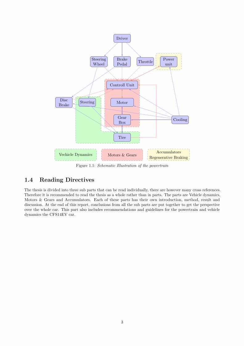
A car can be simplified to four wheels attached to a body with a specified centre of gravity, CoG, illustratedin figure 3.2 from [Jac12]. When a car is accelerating the CoG will generate a force backwards due to its massinertia see figure 3.3. This forces combined with the force generated by the driven wheels will generate a torque

8

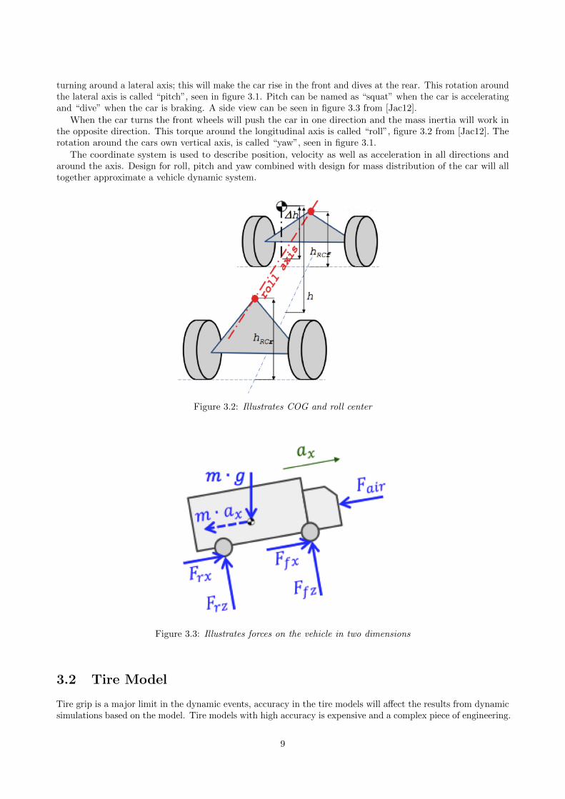
turning around a lateral axis; this will make the car rise in the front and dives at the rear. This rotation aroundthe lateral axis is called “pitch”, seen in figure 3.1. Pitch can be named as “squat” when the car is acceleratingand “dive” when the car is braking. A side view can be seen in figure 3.3 from [Jac12].

When the car turns the front wheels will push the car in one direction and the mass inertia will work inthe opposite direction. This torque around the longitudinal axis is called “roll”, figure 3.2 from [Jac12]. Therotation around the cars own vertical axis, is called “yaw”, seen in figure 3.1.

The coordinate system is used to describe position, velocity as well as acceleration in all directions andaround the axis. Design for roll, pitch and yaw combined with design for mass distribution of the car will alltogether approximate a vehicle dynamic system.

Figure 3.2: Illustrates COG and roll center

Figure 3.3: Illustrates forces on the vehicle in two dimensions

3.2 Tire Model

Tire grip is a major limit in the dynamic events, accuracy in the tire models will affect the results from dynamicsimulations based on the model. Tire models with high accuracy is expensive and a complex piece of engineering.

9

The model used in the dynamic event is a linear equation with a coefficient µ of 1.5. A linear model as equation3.3 is an approximation. All dynamic simulations in this thesis use the same tire model.

Higher degree approximations could be described by the equations 3.1 and 3.2. Higher accuracy is a projectfor future work.

Fx = aFz − bF 2z (3.1)

Fy = aFz − bF 2z (3.2)

3.2.1 Friction Circle

The friction circle shows how much force one tire can handle before losing grip when combining lateral andlongitudinal forces. The model is described by a circle where the circle-line represent the maximum force thetire can handle, i.e. there are no slip within the circle, see figures 3.4 and 3.5. The resulting longitudinal andlateral force is described by the grey arrow in figure 3.4 and 3.5. It should be mentioned that the friction circlealmost always is formed as an ellipse and not a circle.

F 2 = F 2X + F 2

Y ≤ (µFZ)2 → (FX/FZ)2 + (FY /FZ)2 ≤ µ2 (3.3)

Equation 3.3 describes the circle line in the model. The maximum resultant friction force is described byµFZ . Fx, Fy and Fz are the forces that affects the tire. Fx is the lateral force, it varies when the vehicle steers,Fy is the longitudinal force, it’s varies depending on acceleration and braking. For maximum accelerationperformance the resultant arrow should be at the circle line as much as possible, this means the maximumperformance is utilised.

Figure 3.4: Illustation of tire friction circle when accelerating and lateral force to the right

10

Figure 3.5: Illustration of tire friction circle when braking and lateral force to the left

3.3 Vertical Dynamics

Vertical dynamics covers the area of how vertical movements effects the over all vehicle dynamics. By shiftingmass from the body to the wheels, vertical dynamics will be directly affected. This is interesting when discussingimplementation of in-wheel motors.

3.3.1 Method

Figure 3.6: Model illustrates one wheel suspension system

This section will study how different sprung/unsprung masses affects performance of the car. The goal isto evaluate if in-wheel motor is a good alternative to chassis mounted motor despite it’s increased unsprungmass. Values are the same through the separate models, seen in table 3.1. The values in the table are partlyapproximated values and based on CFS12 car. Each motor has an estimated mass of 10 kg. The body massis 270 kg with motors mounted in the chassis and therefore a mass of 250 kg when the motors is mountedin the wheels, assuming 2 motors (RWD). The mass of the wheel is considered as unsprung mass and themass of 1/4 body is considered sprung mass. Three models were made to analyse the vertical dynamics fromdifferent perspectives, visualised in figure 3.6. Model 1 study the response time of chassis when a vehicle hitsunevenness on the track. Model 2 studies a vertical step from the car, this means the suspension is pusheddown 10 mm and then released. This could demonstrate an initial steering step from the driver or a pitchduring acceleration/braking. This is done to evaluate frequency and time to stabilise of the chassis and thewheel. Model 3 was made to analyse the normal forces in between track and tire. Normal force between tireand track is relevant due to its significant impact on traction.

11

Table 3.1: Variable description

Variable Motor in chassis Motor in wheel Unit Descriptionm1 270/4 250/4 kg Sprung massm2 13 23 kg Unsprung massK1 40 40 N/mm Spring constantK2 40 40 N/mm Spring constantB1 3 3 Ns/mm Damper constantB2 3 3 Ns/mm Damper constant

Simplifications and Assumptions

Some simplifications were done to make it possible to do the calculations. The models represent one wheel anda quarter of the chassis mass; it does not take advantage of any other wheel or movement of the vehicle. Thecalculations do not take into account any load transfer that occur when the body moves. Here the masses ofthe body and wheel are simplified to constants. The springs are defined as linear in all models, which leaves uswith constants to describe the forces they generate. Also the dampers are modelled with a damper constant,they generate the same force in both directions. In the comparison of different masses of chassis and wheel,the same constants for springs and dampers are used. In normal case the dampers and springs optimized fordifferent mass distributions.

Vertical model 1

This model was made in Simulink by using a step-source, a transfer function and a scope, seen in figure 3.7. Thetransfer function presented in equation 3.4 was designed using a simple model of one wheel with suspension andchassis shown in figure 3.6. These calculations show the movement of the chassis when the wheel hits a smallstep. G1 = Y1/X, where Y1 is the position of the body and x is the input from the road. G1 is the transferfunction and can be seen in equation 3.4. All variables used are defined in table 3.1. The program makes it

Figure 3.7: Illustrates the Simulink model

possible to plot both the input and output signal in the same graph. A bump is made using a step-source as aninput with a height of 10 mm and a width of 0.5 seconds.

G1(s) =(K2 +B2s)(B1s+K1)

(m1s2 +B1s+K1)(m2s2 +B1s+K1 +K2 +B2s)− (B1 +K1)2(3.4)

Vertical model 2

The second model was set up in Matlab to show how long it takes for the wheel to response from movement ofthe body. The in-data is connected to the vertical position of the body and the desired output is the positionof the wheel. The body has an offset starting position of 10 mm and goes back to its equilibrium when released.The system is presented in figure 3.6. It is possible to study the effects on the wheel by plotting the movementsof the two masses. All constants can be seen in table 3.1. The Matlab program is based on a eigenvalue systemof dynamical oscillations, the both masses represent one wheel and quarter of the body mass visualised infigure 3.6.

12

Vertical model 3

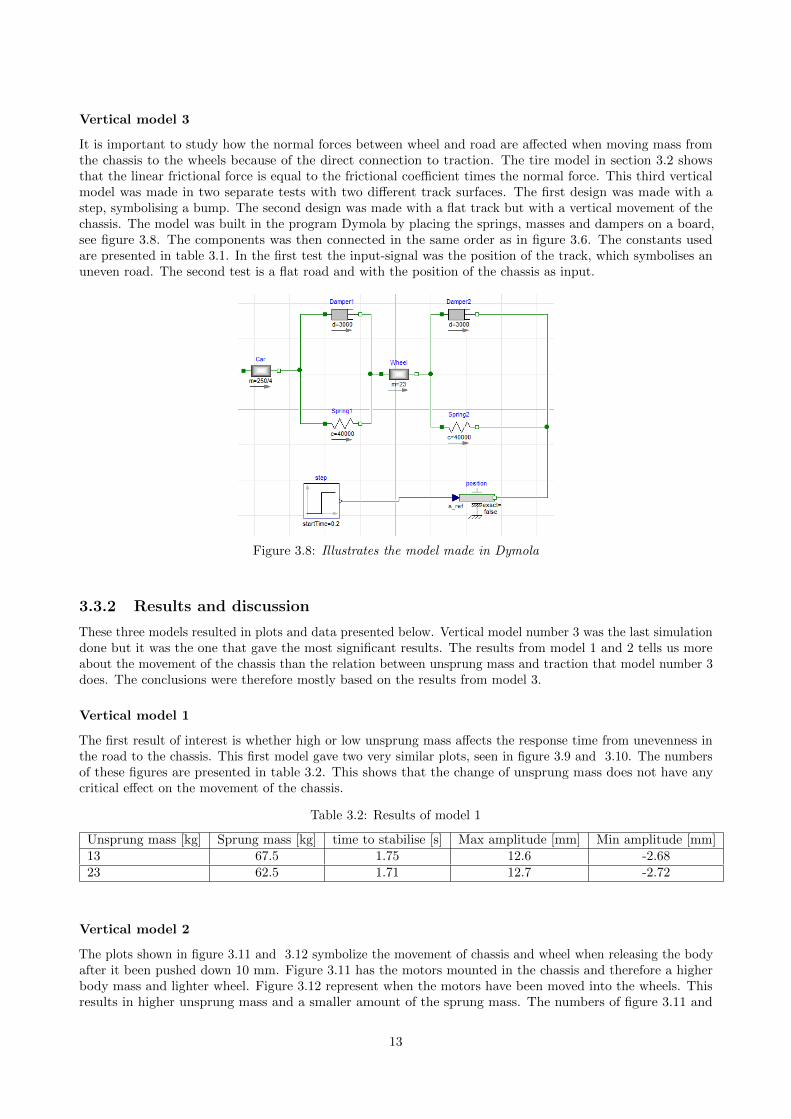
It is important to study how the normal forces between wheel and road are affected when moving mass fromthe chassis to the wheels because of the direct connection to traction. The tire model in section 3.2 showsthat the linear frictional force is equal to the frictional coefficient times the normal force. This third verticalmodel was made in two separate tests with two different track surfaces. The first design was made with astep, symbolising a bump. The second design was made with a flat track but with a vertical movement of thechassis. The model was built in the program Dymola by placing the springs, masses and dampers on a board,see figure 3.8. The components was then connected in the same order as in figure 3.6. The constants usedare presented in table 3.1. In the first test the input-signal was the position of the track, which symbolises anuneven road. The second test is a flat road and with the position of the chassis as input.

Figure 3.8: Illustrates the model made in Dymola

3.3.2 Results and discussion

These three models resulted in plots and data presented below. Vertical model number 3 was the last simulationdone but it was the one that gave the most significant results. The results from model 1 and 2 tells us moreabout the movement of the chassis than the relation between unsprung mass and traction that model number 3does. The conclusions were therefore mostly based on the results from model 3.

Vertical model 1

The first result of interest is whether high or low unsprung mass affects the response time from unevenness inthe road to the chassis. This first model gave two very similar plots, seen in figure 3.9 and 3.10. The numbersof these figures are presented in table 3.2. This shows that the change of unsprung mass does not have anycritical effect on the movement of the chassis.

Table 3.2: Results of model 1

Unsprung mass [kg] Sprung mass [kg] time to stabilise [s] Max amplitude [mm] Min amplitude [mm]13 67.5 1.75 12.6 -2.6823 62.5 1.71 12.7 -2.72

Vertical model 2

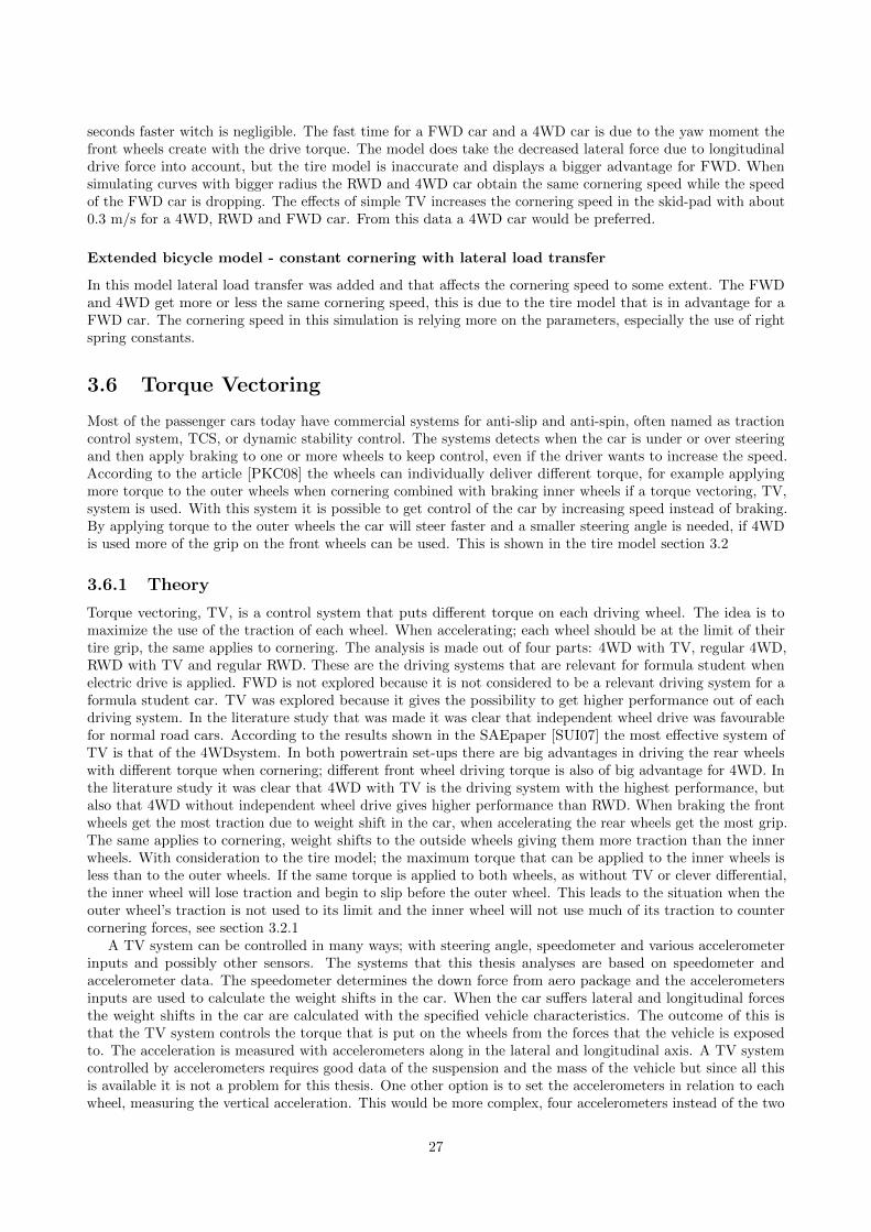
The plots shown in figure 3.11 and 3.12 symbolize the movement of chassis and wheel when releasing the bodyafter it been pushed down 10 mm. Figure 3.11 has the motors mounted in the chassis and therefore a higherbody mass and lighter wheel. Figure 3.12 represent when the motors have been moved into the wheels. Thisresults in higher unsprung mass and a smaller amount of the sprung mass. The numbers of figure 3.11 and

13

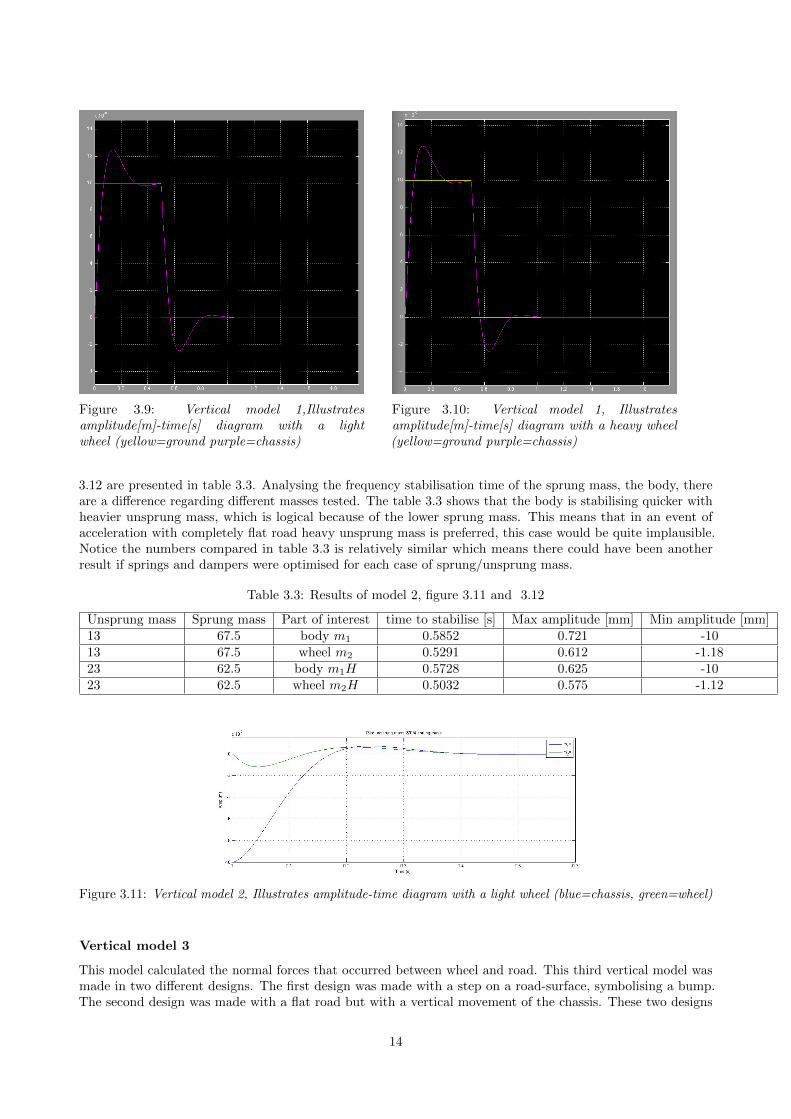
Figure 3.9: Vertical model 1,Illustratesamplitude[m]-time[s] diagram with a lightwheel (yellow=ground purple=chassis)

Figure 3.10: Vertical model 1, Illustratesamplitude[m]-time[s] diagram with a heavy wheel(yellow=ground purple=chassis)

3.12 are presented in table 3.3. Analysing the frequency stabilisation time of the sprung mass, the body, thereare a difference regarding different masses tested. The table 3.3 shows that the body is stabilising quicker withheavier unsprung mass, which is logical because of the lower sprung mass. This means that in an event ofacceleration with completely flat road heavy unsprung mass is preferred, this case would be quite implausible.Notice the numbers compared in table 3.3 is relatively similar which means there could have been anotherresult if springs and dampers were optimised for each case of sprung/unsprung mass.

Table 3.3: Results of model 2, figure 3.11 and 3.12

Unsprung mass Sprung mass Part of interest time to stabilise [s] Max amplitude [mm] Min amplitude [mm]13 67.5 body m1 0.5852 0.721 -1013 67.5 wheel m2 0.5291 0.612 -1.1823 62.5 body m1H 0.5728 0.625 -1023 62.5 wheel m2H 0.5032 0.575 -1.12

Figure 3.11: Vertical model 2, Illustrates amplitude-time diagram with a light wheel (blue=chassis, green=wheel)

Vertical model 3

This model calculated the normal forces that occurred between wheel and road. This third vertical model wasmade in two different designs. The first design was made with a step on a road-surface, symbolising a bump.The second design was made with a flat road but with a vertical movement of the chassis. These two designs

14

Figure 3.12: Vertical model 2, Illustrates amplitude-time diagram with a heavy wheel (blue=chassis, green=wheel)

are represented by test 1 and 2. The x-axis represents time [s] and the y-axis represents force [N]. The normalforce has a start value of 0 Newton, this means that the normal force while rest is not included.

Model 3. Test 1 This test represents a vehicle hitting a bump. Figure 3.13 and 3.14 shows that the normalforces gets a higher peak amplitude and a lower lowest amplitude when the unsprung mass is increased, seetable 3.4. The normal forces can usually be directly transferred to traction between wheel and road but ittakes some time for a tire to deform and build up grip according to [Jac12]. When a wheel bounces with highfrequency is there no chance for the tire to build up grip even if the normal force is high. The wheel willtherefore not be able to take advantage of the extra normal force gained during the first moment hitting thebump. A system with high unsprung mass gets a higher value of negative normal force and a longer time tostabilise compared to a similar system with less unsprung mass, this shows that a lighter wheel handles avertical movement better in this first test in model 3.

Table 3.4: Results of model 3 over bump, figure 3.13 and 3.14

Unsprung mass [kg] Sprung mass [kg] time to stabilise [s] Max amplitude [N] Min amplitude [N]13 67.5 0.0296 3714 -28723 62.5 0.0364 4099 -454

Figure 3.13: Vertical model 3, Amplitude[N]-time[s] with a light wheel over bump

Model 3. Test 2 Figure 3.15 and 3.16 visualise how the normal forces is changing when the chassis ispushed down 10 mm. This should illustrate the squat movement when the vehicle accelerate or brakes. Intable 3.5 are numbers from the plots presented. This test shows that a system with low unsprung mass giveshigher normal force peak amplitude and a shorter time to stabilise. Even if the vehicle is not able to takeadvantage of all the normal force because of the short time that it is increased is still a benefit for the tractionwith higher normal force and a short time for the wheel to stabilize. This test shows that low unsprung mass isto prefer to maximise the vehicles traction.

15

Figure 3.14: Vertical model 3, Amplitude[N]-time[s] with a heavy wheel over bump

Figure 3.15: Vertical model 3, Amplitude[N]-time[s] with a light wheel during acceleration/braking

Figure 3.16: Vertical model 3, Amplitude[N]-time[s] with a heavy wheel during acceleration/braking

Table 3.5: Results of model 3 when accelerating/braking, figure 3.15 and 3.16

Unsprung mass [kg] Sprung mass [kg] time to stabilise [s] Max amplitude [N] Min amplitude [N]13 67.5 0.021 1977 20023 62.5 0.035 1624 200

Discussion

A lot of work is spent on minimizing the unsprung mass when designing a racing vehicle. The results from thevertical model tests describes in some way why. Low unsprung mass makes the wheels adapt and follow the

16

road in a better way, which is seen in the results from vertical model 3. Adaptability results in satisfactorygrip, which is symbolized by the normal force in the two different types of tests in vertical model 3. Grip isdesirable when transferring power from the motors down to the ground and to keep traction when corneringin high speeds. The vertical dynamics analysis was made to make a basis for the placement of motors. Thealternatives were to mount the motors in the chassis or in the wheels. The unsprung mass gets higher if themotors are mounted in the wheels and lower if they are placed in the chassis. After reviewing all the models inthe vertical dynamics, it is concluded that the vehicle, if possible, should be designed so that the motors do notincrease unsprung mass. This is for the vehicle to get as good traction as possible. Model 1 and 2 did not giveany satisfactory results; it was not possible to make any conclusion out of the numbers and plots from these.The effect of changing the unsprung and sprung mass in these models was small and could be an side effect ofall the simplifications made. Therefore was model 3 the only model in this section that gave accurate resultswith clear effects of unsprung mass.

3.4 Longitudinal Dynamics

Modelling of the longitudinal dynamics were done to determine the acceleration ability difference between 4WDand RWD. The model where also used to analyse the demands of the powertrain during maximum accelerationand the load transfer during acceleration and deceleration.

3.4.1 Method

Longitudinal load transfer

This is the model used for the longitudinal load transfer. It does not take suspension geometry, rolling causedby air resistance, damper and spring constants into account. The formula is derived from figure 3.17, takemoment of equilibrium around front and rear were the tyre touches the ground see equation 3.5 to 3.6.

Moment of equilibrium rear. Fzf = m(glr

lf + lr− ax

h

lf + lr) (3.5)

Moment of equilibrium front. Fzr = m(glf

lf + lr+ ax

h

lf + lr) (3.6)

Figure 3.17: Longitudinal load transfer. [Jac12, p.111]

Acceleration model

The electrical powertrain should be designed so that the car will be able to match the best teams. From thefastest times from last year’s acceleration event in Germany 2012, technical requirements have been analysed.The important parameters are the mass of the car with driver, motor torque, gearing and friction coefficient.

17

Most importantly the model indicates the trends, when changing one parameter and keeping the otherconstant and how will this affect the acceleration.

To evaluate the characteristics needed for this event a mathematical model over the acceleration for the carhave been done, see equation 3.7.

Acceleration: a =1

m(Fmotor − Fd − Fr) (3.7)

Where the following forces have been calculated as equation 3.8 to 3.10.

Force: Fmotor =T

Rwheel(3.8)

where the Rwheel is the radius of the wheels.

Drag force: Fd =cdApV

2

2(3.9)

Rolling resistance: Fr = mgk2 (3.10)

Where cd = Drag Coefficient, Ap = Projected area and k2 = rolling resistance. With equations 3.8,3.9, 3.10equation can be written 3.7 can be written as a second degree differential equation, see equation 3.11.

a =1

m

d2s

dt2=

1

m

(T

R− cdAp

2

(ds

dt

)2

−mgk2

)(3.11)

The forces of the aero package are approximated using data given from simulations on CFS12 car and shownin equation. The point of attack is approximated to be in the middle of the car 3.12.

Fdown ≈ 2Fd (3.12)

The gear ratio have been calculated from the speed over the finish line and the maximum rotations perseconds on the motor, see equation 3.13.

gear ratio: ig =ωMaxMotor

ωMaxWheel(3.13)

The torque required from each motor is calculated from the gear ratio ig and wheel torque with equation3.14.

Torque per motor: TMotor =TWheel

ig(3.14)

Assumptions and simplifications

The model have some simplifications. The rolling resistance is assumed to be proportional to the mass of thecar. There are other parameters that also affect but the differences are small [CD79]. It also turns out that theresistance is small in comparison with the driving force. The drag force is increasing with the square of thespeed, which is a common assumption in fluid dynamics [Whi11]. The proportional constant of the drag forceis taken from the analysis of CFS12 car. The moment of inertia in the wheels is not accounted for.

The limits of the race car are the following peak values:

• Maximum power consumption of 85kW with a variable efficiency of the powertrain. The power consump-tion is calculated as torque times rotational speed on the wheel with the efficiency losses.

Power Consumption =Tout ωwheel

ηpower train(3.15)

• Maximum possible torque that one wheel can deliver have been calculated by the the normal force ofeach wheel. The normal force Fnof changes due to load transfer during acceleration and the down forcefrom the aero package . For the moment the friction coefficient of the tire is put to a constant at µtire.

Twheel = FnµtireRwheel (3.16)

18

• The motor is a PMSM(permanent magnet synchronous motor) and the torque will be limited when themotor reaches the rated speed, which after field weakening is used see subsection 4.3.2.

• General data is taken from the CFS12 car since the new one have not been built nor tested.

3.4.2 Result

Here are the results from longitudinal dynamics

Results from acceleration model

0 0.5 1 1.5 2 2.5 3 3.50

10

20

30

40

50

60

70

time [s]

Distance [m]speed [m/s]

Acceleration [m/s2]

(a) 4WD

0 0.5 1 1.5 2 2.5 3 3.5 40

10

20

30

40

50

60

70

time [s]

Distance [m]speed [m/s]

Acceleration [m/s2]

(b) 2WD

Figure 3.18: Distance, Speed and Acceleration during a Acceleration Event

A comparison of 2WD and 4WD in the acceleration event is illustrated in figure 3.33. The data from themodel indicates that the 4WD is 0.38 s faster in the acceleration event than RWD. This will give a difference inscore of 17 points if the same vehicle as last year would compete with the rules of 2013. The assumption is thatthe motor, gearing and motor controller for the front wheel in a 4WD car will increase the weigh of the carwith ∼ 25kg. There’s a gain in acceleration with 4WD because of the possibility in using the traction in thefront wheels which otherwise is unused.

Table 3.6: Results from model

2WD 4WDMass [kg] 293 318.00Time [s] 3.85 3.47Max Speed [Km/h] 128.5 131Torque Front [Nm] 0.00 223Torque Back [Nm] 429 460Max power [kW] 85 85Max rear distribution 0.73% 0.81%

The potential greatest error is the tyre model. Since the tyre grip is the biggest limit of the performance, abasic tyre model will reduce the accuracy of the results. With this tire model the grip increase linearly withthe down force. The load transfer do not take the pitch into account and this reduce the difference between

19

front and back weight distribution during acceleration. The efficiency of the system have been approximatedand can therefore differ in a real car. The model also assume that the tire friction is equal on each wheel andthat torque can be even distributed between the wheels. The data shows a approximation of the loads andresults of a acceleration event and will be used in the demands of motors and gears.

3.5 Lateral Dynamics

OptimumLap

OptimumLap is used to get lap times for autocross, endurance, skid-pad and acceleration. Different vehiclemodels that differ in driven axles are used. The results from the simulations is then analysed and it is possibleto see what type of setting is best for the tracks that the car is going to run on. The difference in a 4WD or aRWD car is analysed.

Bicycle model - constant cornering without lateral load transfer

The bicycle model is used to make a simple model of the vehicle and test it in different radius curves andsee what combination of driven wheels makes it achieve highest cornering speed. The different radius curvessimulate the skid-pad and curves that occur in autocross and endurance. Basic TV is also analysed.

Extended bicycle model - constant cornering with lateral load transfer

The bicycle model is used to make a simple model of the vehicle and test it in different radius curves andsee what combination of driven wheels makes it achieve highest cornering speed. The different radius curvessimulate the skid-pad and curves that occur in autocross and endurance. This model also include the effects ofload transfer, this will make it a more complete model.

3.5.1 Method

OptimumLap

OptimumLap was used to simulate the vehicle going around a specific path and stored lap time, speed,acceleration and rpm.

Track

OptimumLap has its own database for tracks [Web] were they have both the Autocross and Endurancetrack from 2012 Germany stored. OptimumLap also has a track maker were the skid-pad and the 0-75 macceleration track was created. These were then used in the simulations.

Vehicle

Creating a vehicle in OptimumLap can be done by very few parameters. It needs: mass, driven wheels, dragcoefficient, down force coefficient, front area, air density, tire radius, rolling resistance, longitudinal friction,lateral friction, engine data, transmission type, gear ratios, final drive ratio and drive efficiency. The usedvalues come from the CFS12 car. With different values for motor data, transmission type, gear ratios, finaldrive ratio and drive efficiency, this data comes from CFS13EV.

Simplifications and assumptions

This is a simplified vehicle dynamics simulating tool and does not look at suspension geometry and uses asimplified tire model. The motor model used is a simplification of the motor used in the CFS13EV. It is notpossible to look at a FWD car in this program so the only comparison is between RWD with 4WD.

20


When analysing vehicle cornering speed it is possible to combine the wheels on one axle to one virtual wheel.This makes it a lot easier to understand and analyse. Even if the model loses some accuracy it can still be usedto analyse vehicle behaviour. The cases that a basic bicycle model cannot handle is yaw moment coming fromdifferent drive torque on the same axle, when the vehicle have large deviation from Ackerman geometry andwhen the cornering stiffness changes under load transfer, though it is possible to model these behaviours withsub-models. Steady state cornering captures cornering at high speed, but only in steady state, typically when avehicle is running on a skid-pad see [Jac12, p.109]. It means that all time a derivative of the vehicles speed iszero, like the lateral speed, longitudinal speed and also the yaw rate. That makes the speeds constant. When

running in a corner the total speed of the vehicle is√

(v2x + v2y) and in this case this is a constant, the yaw rate

wz is also a constant. Then the centripetal acceleration ac = R× w2z = v2/R = wz × v is constant. In figure

3.19 the advanced bicycle model without the simplifications is shown. From this figure equations to analysevehicle behaviour is derived. It is possible to simplify the advanced model (figure 3.19) to create a model thatis easier to understand. The simplification on this easy model is assuming small steering angles and no driveforces see figure 3.20. After cancelling out some variables, two equations are left. One describing the under steer

gradient Ku =Cr×lr−Cf×lf

Cf×Cr×L and one describing how much more or less steering angle df = LR +Ku× m×(vx)

2

R

that is needed if the speed for a specific curve radius is increased. This depends on the sign of the under steergradient and how big it is. When the under steer gradient is smaller then 0 the vehicle is said to be over steeredand if the under steer gradient is larger then 0 it is under steered. An over steered vehicle can become unstableeasier than a under steered vehicle which makes a under steered vehicle preferred but it is not this simplifiedmodel that is used in the simulations.

Compensates corneringstiffness due to drive moment: Crn = Cr ×√

1− (Frx

mu× Frz)2 (3.17)

Compensates corneringstiffness due to drive moment: Cfn = Cf ×

√1− (

Ffxw

mu× Ffz)2 (3.18)

Force vertical to wheel. Ffyw = −Cfn × sfy (3.19)

Force vertical to wheel. Fry = −Crn × sry (3.20)

Force vertical to wheel. sfy =vfywvfxw

(3.21)

Force vertical to wheel. sry =vryvrx

(3.22)

Front axle loses grip first. Ffyw =√

(mu× Ffz)2 − F 2fxw (3.23)

Checking rear axle gripp. mu× Frz >√F 2ry + F 2

rx (3.24)

Tire model

The tire model used in the constant cornering without lateral load transfer model is a relation betweenlateral force and lateral slip, but it also utilizes a roof on the lateral force who is coupled to the longitudinalforce see equation 3.19 to 3.23. The roof on the front axle grip is based on an assumption that front axle willlose grip first, this is then checked by looking at the side force and the longitudinal force on the rear axle seeequation 3.24. Equation 3.17 to 3.18 also captures changes in cornering stiffness due to longitudinal wheelforces, this works rather well but is not completely physically motivated [Jac12, p.50]. The need to use equation3.23 is based on the fact that maximal speed is wanted in the skid-pad. This is achieved when one of the axlesis about to lose grip.

21

Figure 3.19: Advanced one-track model for steady state cornering at high speed. [Jac12, p.111]

Figure 3.20: Simple one-track model for steady state cornering at high speed. [Jac12, p.113]

22

Equations

The model is based on the equations derived from figure 3.19. First the equilibrium see equations 3.25 to3.29 then compatibility see equations 3.30 to 3.33 and transformation between vehicle and wheel coordinatesystems see equations 3.34 to 3.37, these are the main equations needed for the simulation. The vehicle pathwas added to be able to plot the path of the vehicle see [Jac12, p.99]. The simulation was done in Dymola tosimulate cornering speed in different corner radius. The used tire model is presented in equations 3.17 to 3.23.The vehicle parameters needed by the script is: mass, cornering stiffness, g, CoG position, friction coefficient,π, radius of driven circle, relation between front and rear drive torque, vertical normal forces and what axleloses grip first. The model then returns values on speed, acceleration, force, steering angle and position. Themodel also specifies how much torque that goes to the front axle and how much to the rear axle.

Equilibrium force: m× ax = Frx + Ffxv (3.25)

Equilibrium force: m× ay = Fry + Ffyv (3.26)

Moment of equilibrium around CoG: J × 0 = Ffyv × lf − Fry × lr (3.27)

Equilibrium speed: − ax = vy × wz (3.28)

Equilibrium speed: ay = vx × wz (3.29)

Compatibility: vfxv = vx (3.30)

Compatibility: vfyv = vy + wz × lf (3.31)

Compatibility: vrx = vx (3.32)

Compatibility: vry = vy − wz × lr (3.33)

Transformation between vehicle and wheel coordinate systems: Ffxv = Ffxw × cos(df)− Ffyw × sin(df)(3.34)

Transformation between vehicle and wheel coordinate systems: Ffyv = Ffxw × sin(df) + Ffyw × cos(df)(3.35)

Transformation between vehicle and wheel coordinate systems: vfxv = vfxw×cos(df)−vfyw×sin(df) (3.36)

Transformation between vehicle and wheel coordinate systems: vfyv = vfxw×sin(df)+vfyw×cos(df) (3.37)


This model does not include lateral load transfer; this means that it is not possible to see the differentnormal forces on the right and the left wheel during cornering. A simplified model of a tire is that the wheelforces vary with the normal forces. This will then vary the cornering stiffness, the cornering stiffness candecrease when the load transfer interfere [Jac12, p.43]. It also does not take suspension linkage and wheelgeometry into account. The effect of the aero package is not looked at. The analysis of the effect that TV hason the lap time is very simplified. The moment that the wheels will create if drive torque to the outer wheels isanalysed is added.

23


This model is an extension of Bicycle model - constant cornering without lateral load transfer. This modeltakes lateral load transfer into account and that is important in a event like skid-pad. When looking at lateralload transfer suspension for front and rear has to be considered independently. How the forces transmit fromthe road to the body and right and left elasticity is important. This means that with a linkage model, theused model is a axle roll center model see figure 3.21. Equations 3.38 to 3.40 is derived from this figure. Themain assumption of the roll centre model is that the roll centre does not have any roll moment. When lookingat constant cornering the dampers will not have any effect because the velocity is zero (F = −d × v). Thesprings are assumed to be linear with a constant c, and the spring travel is measured from a static conditionF = F0 + c× (zr − z), where F is the force in the damper, F0 is the static force, c is the effective stiffness, zr isthe road movement which is set to zero and z is the body movement. The equation is differentiated and to theequations 3.41 to 3.44.

Equilibrium for roll: 0 = (Fflz + Frlz)× w

2− (Ffrz + Frrz)× w

2+ (Ffy + Fry)× h (3.38)

Equilibrium for the axles around front roll centre: 0 = (Fflz − Fsfl)×w

2− (Ffrz − Fsfr)× w

2+ Ffy × hRCf

(3.39)

Equilibrium for the axles around rear roll centre: 0 = (Frlz−Fsrl)×w

2−(Frrz−Fsrr)×w

2+Fry×hRCr (3.40)

Compatibility: vflz =w

2× wx (3.41)

Compatibility: vfrz = −w2× wx (3.42)

Compatibility: vrlz =w

2× wx (3.43)

Compatibility: vrrz = −w2× wx (3.44)


This model does not include the effects of the aero package; it also utilizes a very simplified tire model. Thespring constants are estimations based on the CFS12 car. The roll centre model has some drawbacks: it is notoptimal for large load transfer like roll-over and wheel lift, it should not be used when looking at heave and notwhen big difference in longitudinal slip occur. It also has some advantages over the model with wheel pivotpoints: it is less computational demanding see [Jac12, p.127]. This model does not include damping, heave androll inertial effects that are needed for transient events but that is not the case here.

3.5.2 Results

OptimumLap

Having a 4WD car gives better lap times on autocross, endurance and acceleration than a RWD car, see table3.7. These results are when the car weighs equally much with RWD and 4WD. If 25 kg (assumed) is added tothe car with 4WD different lap times are reached see table 3.7, but even then the 4WD beats RWD. Theseresults are from the autocross and endurance tracks from 2012 in Germany. All these results are in favour for a4WD car.

24

Figure 3.21: Axle roll centre model. [Jac12, p.127]

Table 3.7: OptimumLap Results

Lap Times4WD/RWD Autocross [s] Endurance [s] Acceleration [s] Skid-pad [s]4WD 69 77 3.9 4.77RWD 72 82 4.7 4.774WD (25 kg) 70 78 4.1 4.77


The main results from the Bicycle model - constant cornering without lateral load transfer model is themaximum speed that can be obtained in the skid-pad. The maximum speed for a RWD car is 11.14 m/s. For a4WD car it is 11.21 m/s and for a FWD car 11.22 m/s. Some other constant curves that occur in autocrossand endurance was also simulated see table 3.8. The path of the vehicle is illustrated in figure 3.22. If theeffect of TV as a moment on the car due to different drive forces on left and right side is added, different datais gathered see table 3.9.

Table 3.8: Bicycle model - constant cornering without lateral load transfer Data

Longitudinal Speed4WD/RWD/FWD Skid-pad (D=17.1m) [m/s] (D=23m) [m/s] (D=45m) [m/s] (D=54m) [m/s]RWD 11.14 12.97 18.19 19.934WD 11.21 13.01 18.20 19.93FWD 11.22 13.00 18.11 19.82

25

Table 3.9: Bicycle model - constant cornering without lateral load transfer and with TV Data

Longitudinal Speed4WD/RWD/FWD Skid-pad (D=17.1m) [m/s]RWD 11.444WD 11.50FWD 11.50

Figure 3.22: Path in the skid-pad. [Jac12, p.113]


From table 3.10, the RWD car has the lowest speed in the skid-pad event. The FWD car and the 4WD carhave more or less the same speed. So from this data a 4WD or FWD car would be preferred.

Table 3.10: Extended bicycle model - constant cornering with lateral load transfer Data

Longitudinal Speed4WD/RWD/FWD Skid-pad (D=17.1m) [m/s] (D=23m) [m/s] (D=45m) [m/s] (D=54m) [m/s]RWD 11.13 12.93 18.13 19.874WD 11.20 13.00 18.19 19.93FWD 11.22 13.02 18.21 19.94

3.5.3 Discussion

OptimumLap

The data from the simulations done in OptimumLap see table 3.7 is in advantage of a 4WD car. This dataonly looks at RWD and 4WD so nothing can be said about RWD and 4WD against FWD. The 4WD car issignificantly faster then the RWD car especially in acceleration. Even with 25 kg of extra weight added to the4WD car the 4WD car still outperform the RWD car in autocross, endurance and acceleration.


From this Bicycle model the difference in cornering speed on a FWD, RWD and 4WD car is analysed. Fromthe data see table 3.8 a 4WD car has the best lap times except for in the skid-pad were the FWD car is 0.01

26

seconds faster witch is negligible. The fast time for a FWD car and a 4WD car is due to the yaw moment thefront wheels create with the drive torque. The model does take the decreased lateral force due to longitudinaldrive force into account, but the tire model is inaccurate and displays a bigger advantage for FWD. Whensimulating curves with bigger radius the RWD and 4WD car obtain the same cornering speed while the speedof the FWD car is dropping. The effects of simple TV increases the cornering speed in the skid-pad with about0.3 m/s for a 4WD, RWD and FWD car. From this data a 4WD car would be preferred.


In this model lateral load transfer was added and that affects the cornering speed to some extent. The FWDand 4WD get more or less the same cornering speed, this is due to the tire model that is in advantage for aFWD car. The cornering speed in this simulation is relying more on the parameters, especially the use of rightspring constants.

3.6 Torque Vectoring

Most of the passenger cars today have commercial systems for anti-slip and anti-spin, often named as tractioncontrol system, TCS, or dynamic stability control. The systems detects when the car is under or over steeringand then apply braking to one or more wheels to keep control, even if the driver wants to increase the speed.According to the article [PKC08] the wheels can individually deliver different torque, for example applyingmore torque to the outer wheels when cornering combined with braking inner wheels if a torque vectoring, TV,system is used. With this system it is possible to get control of the car by increasing speed instead of braking.By applying torque to the outer wheels the car will steer faster and a smaller steering angle is needed, if 4WDis used more of the grip on the front wheels can be used. This is shown in the tire model section 3.2

3.6.1 Theory

Torque vectoring, TV, is a control system that puts different torque on each driving wheel. The idea is tomaximize the use of the traction of each wheel. When accelerating; each wheel should be at the limit of theirtire grip, the same applies to cornering. The analysis is made out of four parts: 4WD with TV, regular 4WD,RWD with TV and regular RWD. These are the driving systems that are relevant for formula student whenelectric drive is applied. FWD is not explored because it is not considered to be a relevant driving system for aformula student car. TV was explored because it gives the possibility to get higher performance out of eachdriving system. In the literature study that was made it was clear that independent wheel drive was favourablefor normal road cars. According to the results shown in the SAEpaper [SUI07] the most effective system ofTV is that of the 4WDsystem. In both powertrain set-ups there are big advantages in driving the rear wheelswith different torque when cornering; different front wheel driving torque is also of big advantage for 4WD. Inthe literature study it was clear that 4WD with TV is the driving system with the highest performance, butalso that 4WD without independent wheel drive gives higher performance than RWD. When braking the frontwheels get the most traction due to weight shift in the car, when accelerating the rear wheels get the most grip.The same applies to cornering, weight shifts to the outside wheels giving them more traction than the innerwheels. With consideration to the tire model; the maximum torque that can be applied to the inner wheels isless than to the outer wheels. If the same torque is applied to both wheels, as without TV or clever differential,the inner wheel will lose traction and begin to slip before the outer wheel. This leads to the situation when theouter wheel’s traction is not used to its limit and the inner wheel will not use much of its traction to countercornering forces, see section 3.2.1

A TV system can be controlled in many ways; with steering angle, speedometer and various accelerometerinputs and possibly other sensors. The systems that this thesis analyses are based on speedometer andaccelerometer data. The speedometer determines the down force from aero package and the accelerometersinputs are used to calculate the weight shifts in the car. When the car suffers lateral and longitudinal forcesthe weight shifts in the car are calculated with the specified vehicle characteristics. The outcome of this isthat the TV system controls the torque that is put on the wheels from the forces that the vehicle is exposedto. The acceleration is measured with accelerometers along in the lateral and longitudinal axis. A TV systemcontrolled by accelerometers requires good data of the suspension and the mass of the vehicle but since all thisis available it is not a problem for this thesis. One other option is to set the accelerometers in relation to eachwheel, measuring the vertical acceleration. This would be more complex, four accelerometers instead of the two

27

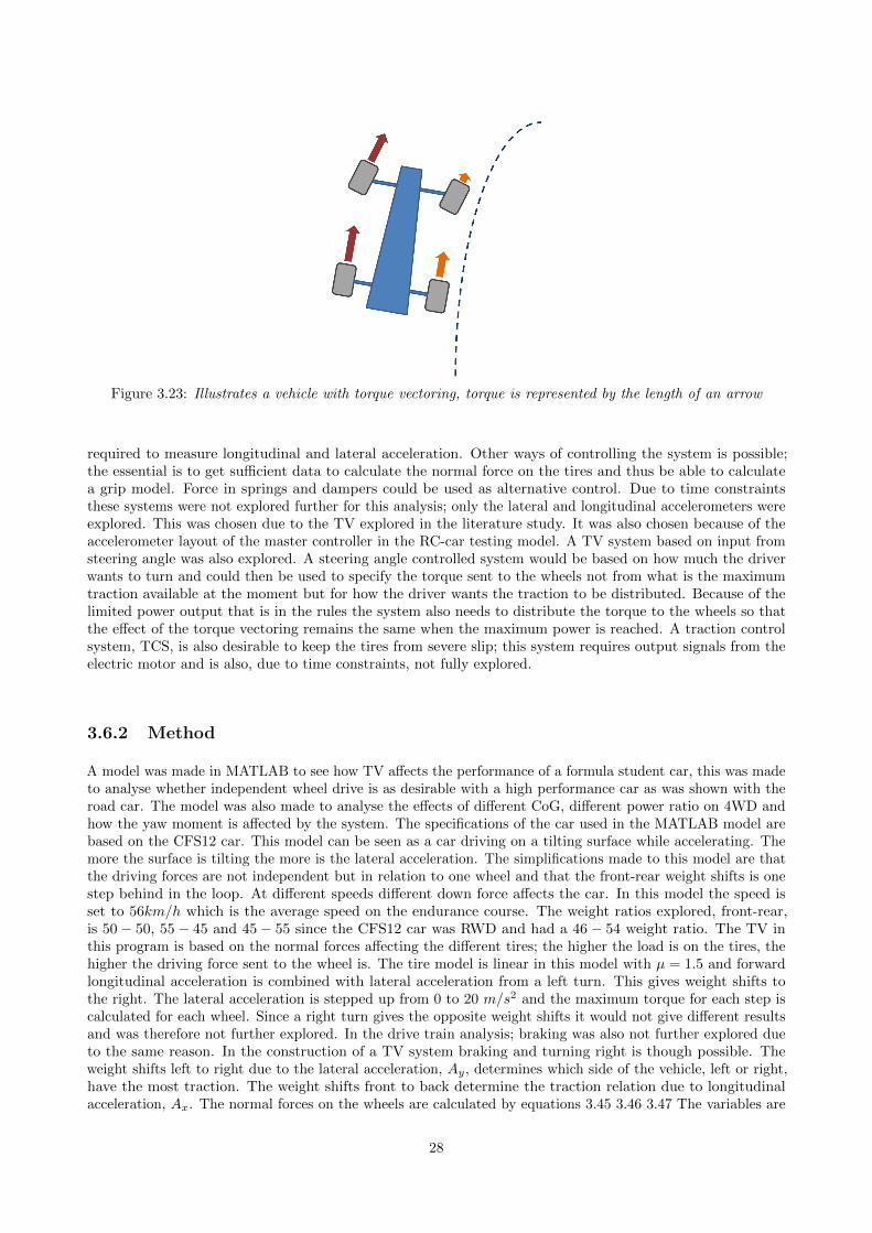
Figure 3.23: Illustrates a vehicle with torque vectoring, torque is represented by the length of an arrow

required to measure longitudinal and lateral acceleration. Other ways of controlling the system is possible;the essential is to get sufficient data to calculate the normal force on the tires and thus be able to calculatea grip model. Force in springs and dampers could be used as alternative control. Due to time constraintsthese systems were not explored further for this analysis; only the lateral and longitudinal accelerometers wereexplored. This was chosen due to the TV explored in the literature study. It was also chosen because of theaccelerometer layout of the master controller in the RC-car testing model. A TV system based on input fromsteering angle was also explored. A steering angle controlled system would be based on how much the driverwants to turn and could then be used to specify the torque sent to the wheels not from what is the maximumtraction available at the moment but for how the driver wants the traction to be distributed. Because of thelimited power output that is in the rules the system also needs to distribute the torque to the wheels so thatthe effect of the torque vectoring remains the same when the maximum power is reached. A traction controlsystem, TCS, is also desirable to keep the tires from severe slip; this system requires output signals from theelectric motor and is also, due to time constraints, not fully explored.

3.6.2 Method

A model was made in MATLAB to see how TV affects the performance of a formula student car, this was madeto analyse whether independent wheel drive is as desirable with a high performance car as was shown with theroad car. The model was also made to analyse the effects of different CoG, different power ratio on 4WD andhow the yaw moment is affected by the system. The specifications of the car used in the MATLAB model arebased on the CFS12 car. This model can be seen as a car driving on a tilting surface while accelerating. Themore the surface is tilting the more is the lateral acceleration. The simplifications made to this model are thatthe driving forces are not independent but in relation to one wheel and that the front-rear weight shifts is onestep behind in the loop. At different speeds different down force affects the car. In this model the speed isset to 56km/h which is the average speed on the endurance course. The weight ratios explored, front-rear,is 50 − 50, 55 − 45 and 45 − 55 since the CFS12 car was RWD and had a 46 − 54 weight ratio. The TV inthis program is based on the normal forces affecting the different tires; the higher the load is on the tires, thehigher the driving force sent to the wheel is. The tire model is linear in this model with µ = 1.5 and forwardlongitudinal acceleration is combined with lateral acceleration from a left turn. This gives weight shifts tothe right. The lateral acceleration is stepped up from 0 to 20 m/s2 and the maximum torque for each step iscalculated for each wheel. Since a right turn gives the opposite weight shifts it would not give different resultsand was therefore not further explored. In the drive train analysis; braking was also not further explored dueto the same reason. In the construction of a TV system braking and turning right is though possible. Theweight shifts left to right due to the lateral acceleration, Ay, determines which side of the vehicle, left or right,have the most traction. The weight shifts front to back determine the traction relation due to longitudinalacceleration, Ax. The normal forces on the wheels are calculated by equations 3.45 3.46 3.47 The variables are

28

explained in tabular 3.24

dWyf = mfAy(Hg/(1 +Kr/Kf −mfHg/Kf ) + LrHf/L)/Wf (3.45)

dWx = mAxHg/L (3.46)

Wfl = mf/2g − dWyf − dWx/2 +Aerof/2 (3.47)

The fl index is front left, fr is front right, rl is rear left and rr is rear right. The grip of each wheel is thencalculated with equation 3.48

Rfl = µWfl (3.48)

These formulas combined give the total traction of each wheel, R. The radius of the traction circle R is thenused to calculate what the available traction for lateral and longitudinal forces are. The driving force put onthe wheels is the relation between the traction circles and is calculated by equation 3.49

Dfl = DrrRfl

Rrr(3.49)

The driving force on the right rear wheel, the wheel with the most traction, determines the torque givento each other wheel. When the driving force is stepped up the remaining grip to take up the lateral load iscalculated by equation 3.50

Cfl =√

(R2fl −D2

fl) (3.50)

The maximum torque of each wheel is calculated so that there is enough traction to take up the lateral load.In the analysis part, the longitudinal acceleration is calculated by the torque on each wheel. In the runningTV program used with the RC-car the longitudinal acceleration is an input from the accelerometer. Whenthe lateral acceleration force becomes too great the driving force is shut off and the traction is only used forcornering. In the regular models the driving force on the tire is the same left and right and split differently onthe front and rear wheels in 4WD mode. To make for a fair comparison between the powertrains the differentratios of 4WD were explored to find the front wheel drive ratio that gives the highest performance. The testedratio ranges from 20% to 50% of drive on the front wheels. The maximum torque of each wheel and eachsystem is given for the range of lateral acceleration. The longitudinal acceleration achieved is also collected.To get clear results the weight distribution was kept at 50-50 front-rear for the part where the four differentpowertrains, 4WD with TV, 4WD, RWD with TV and RWD are compared. The comparison between the yawmoment of the TV system was made with equations 3.51 3.52 3.53

YMf = (Dfr −Dfl)Wf/2 (3.51)

YMr = (Drr −Drl)Wr/2 (3.52)

YM = YMf + YMr (3.53)

The comparisons between the powertrains were made to show clear result of what driving systems gave thehighest performance. The area under the longitudinal-lateral acceleration plots were calculated as this reflectsthe cars ability to accelerate while cornering. This gives the car better performance exiting a corner. To makefor a comparison the highest number was set to one and the other systems ranges from zero to one. The samewere done for the 4WD systems to show which front wheel drive ratio gave the best performance; here the4WD with TV was set as the reference drive system.

29

Figure 3.24: Explanation of the variables used

dWyf Weight shifts front due to lateral load L Length of vehiclemf Front mass Wf Front treadGy Lateral acceleration dWx Weigth shifts due to longitudinal loadHg Height of COG m Mass of vehicleKr Front roll stiffness Gx Longitudinal accelerationKf Rear roll stiffness Wfl Normal force on front left tireLr Length from COG to rear Dfl Driving force on front left tireHf Height of front roll center YMf Front yaw moment

0 5 10 15 200

500

Wheel to

rque [N

m]

4WD Torque Vectoring

Lateral acceleration [m/s2]

0 5 10 15 200

20

0 5 10 15 200

5004WD No T−V

lateral acceleration [m/s2]

0 5 10 15 200

20

Longitudin

al accele

ration [m

/s2]

Front left

Front right

Rear left

Rear right

0 5 10 15 200

200

400

600

Wheel to

rque [N

m]

RWD Torque Vectoring


0 5 10 15 200

5

10

15

0 5 10 15 200

200

400

600RWD No T−V


0 5 10 15 200

5

10

15

Longitudin

al accele

ration [m

/s2]

Rear left

Rear right

Figure 3.25: Torque distribution between wheels for combined forward acceleration and left cornering acceleration

3.6.3 Results

Figure 3.25 shows the torque of each wheel in relation to the achieved lateral acceleration and longitudinalacceleration of each driving system. The systems without TV gives the same power to the wheels, wheel pairsin 4WD, and the torque is set to zero when it exceeds the traction. The shut off system is the reason that thelines are bumpy in the non-torque vectoring systems. This shows that the most torque can be put down whenusing TV and that 4WD with TV is the system with the highest performance.

Figure 3.26 shows the difference in combined longitudinal and lateral acceleration achieved with differentdriving systems. For 4WD the ratio of 20%-80% front-rear driving ratio is applied, this is the one with thehighest performance. This plot shows that 4WD with TV is the best system.

Figure 3.27 shows the difference in yaw moment from the TV systems of 4WD and RWD. Yaw momentfrom steering angle is not taken into account in this plot. 4WD with TV gives the highest yaw moment.

Figure 3.28 shows the difference between different weight distributions of the driving systems. The plotshows what longitudinal acceleration can be achieved while under a lateral load. This shows that 4WD withTV and a 50− 50 weight distribution is the system with the highest performance.

Figure 3.29 is a comparison between the systems of how much combined longitudinal and lateral accelerationcan be achieved. The bar chart shows the relation of the areas under the longitudinal-lateral-acceleration plots.This shows that 4WD with TV and a 50 − 50 weight distribution gives the highest capability to acceleratewhile cornering.

Figure 3.30 shows the difference in combined acceleration capabilities between different ratios of front wheeldrive for the 4WD regular model. 1 is the 4WD with TV value. This shows that 20% front wheel drive wouldgive the highest performance.

30

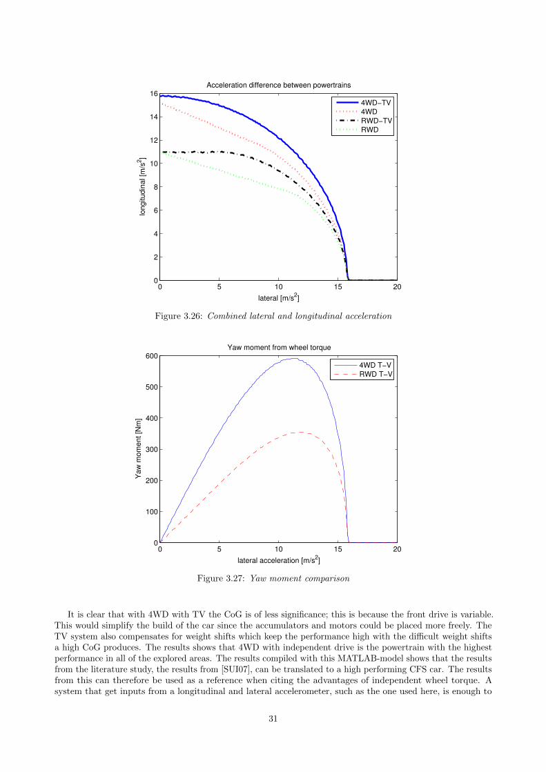
0 5 10 15 200

2

4

6

8

10

12

14

16

lateral [m/s2]

longitudin

al [m

/s2]

Acceleration difference between powertrains

4WD−TV

4WD

RWD−TV

RWD

Figure 3.26: Combined lateral and longitudinal acceleration

0 5 10 15 200

100

200

300

400

500

600


Yaw

mom

ent [N

m]

Yaw moment from wheel torque

4WD T−V

RWD T−V

Figure 3.27: Yaw moment comparison

It is clear that with 4WD with TV the CoG is of less significance; this is because the front drive is variable.This would simplify the build of the car since the accumulators and motors could be placed more freely. TheTV system also compensates for weight shifts which keep the performance high with the difficult weight shiftsa high CoG produces. The results shows that 4WD with independent drive is the powertrain with the highestperformance in all of the explored areas. The results compiled with this MATLAB-model shows that the resultsfrom the literature study, the results from [SUI07], can be translated to a high performing CFS car. The resultsfrom this can therefore be used as a reference when citing the advantages of independent wheel torque. Asystem that get inputs from a longitudinal and lateral accelerometer, such as the one used here, is enough to

31

0 5 10 15 200

5

10

15

20

lateral [m/s2]

longitudin

al [m

/s2]

4WD−TV different weight distribution

50F−50R

55F−45R

45F−55R

0 5 10 15 200

5

10

15

20

lateral [m/s2]

longitudin

al [m

/s2]

4WD different weight distribution

50F−50R

55F−45R

45F−55R

0 5 10 15 200

5

10

15

lateral [m/s2]

longitudin

al [m

/s2]

RWD−TV different weight distribution

50F−50R

55F−45R

45F−55R

0 5 10 15 200

5

10

15

lateral [m/s2]

longitudin

al [m

/s2]

RWD different weight distribution

50F−50R

55F−45R

45F−55R

Figure 3.28: COG comparison

4WD−TV . 4WD . RWD−TV . RWD .0

0.1

0.2

0.3

0.4

0.5

0.6

0.7

0.8

0.9

1Comparison of acceleration capabilites between powertrains

50F−50R

55F−45R

45F−55R

Figure 3.29: COG and powertrain comparison

get higher performance from the powertrains. The higher yaw-moment from the TV system can be furtherincreased with a steering angle controlled system. This system can also be implemented as shown in section 3.7.TV is here implemented with four separate motors but for a CFS car it could also be implemented with cleverdifferentials. The important with this type of TV is to calculate the weight shifts in the car and from that putthe most torque on the wheel with the highest normal force put on it. RWD with TV is also desirable but itstill gives lower performance than regular 4WD with 20% of drive on the front wheels. The down force fromthe aero pack is generated at the average speed of 56km/h but at other speeds the results remains the same.

32

15 20 25 30 35 40 45 50 550

0.1

0.2

0.3

0.4

0.5

0.6

0.7

0.8

0.9

1

% front drive

Comparison of acceleration capabilites between 4WD systems

Figure 3.30: 4WD front drive percent comparison

3.7 Physical Testing Vehicle

A model of a race car was made to compare RWD with 4WD and to implement and test TV. Vehicle dynamicsis normally not possible to scale so the goal was not to test the overall handling. The testing vehicle was madeto test the TV system and the principle of having individual motors for each wheel and a master controller.The complexity and problems of implementing such a system were explored and solved as an effect of thebuild. Each group were included during the work with the car model contributing with their own subject. Thecar was not build as a scale of the CFS12 but of parts that we could afford and satisfied the demand of thesystem. The demands of the car were that it should be able to spin on all tires and be able to control eachwheel individually. The master controller needed to be able to handle acceleration and steering angle as inputand have enough calculation power to be able to calculate the torque vectoring program designed. The mastercontroller needed to be able to create a PWM signal that matches the motor controllers input signal. Theparts were mainly chosen for their simplicity and availability. The motors with the highest low speed torquewere bought for available funds.

3.7.1 RC-car TV system.

This system was made to explore the possibilities of TV and to be a basis for the applied TV system used inthe RC-prototype vehicle. The TV system created was based on the same equations as the analyses program.The system is tough made with the possibility of a steering angle controlled system as well as the accelerometercontrolled. The different torque outputs to the wheels can be stored in matrixes and collected by inputs oflateral acceleration and velocity. The TV system can also be controlled by inputs of lateral and longitudinalacceleration, steering angle as well as the velocity to calculate the maximum torque for each wheel constantlyin the program. The main outlines of a TV system were designed to work like this: TV system with inputsfrom accelerometers and velocity/rpm. This determines the maximum torque the wheels can handle due toweight shifts and down force. TCS. This limits the power to the wheel in case of severe slip. This systemcould run of the rpm read of the motors; if a high derivative of the rpm is read the wheel is spinning and thetorque to that wheel should be lowered. This system needs to be calibrated with a more accurate tire model.The system lowers the torque on the inner wheels when turning while accelerating forward, when braking thesystem lowers the braking on the outer wheels. It can also be set up to lower the power to the front wheelswhile turning. Throttle control. This is where the signal from the throttle/brake pedal comes in. It varies thepower sent to each wheel from an input from the driver. This system should lower the power equally on wheel

33

to maintain the increased yaw moment the TV system creates. Power limiter system limits the torque to thewheels in case of a total power that is exceeding the maximum power of 85kw according to the rules.

The maximum torque outputs on each wheel were calculated for combined longitudinal and lateral accelerationwith the specifications of the RC-car. These numbers are presented in figure 3.31. Here 0 represents maximumright turn on the lateral axis and 40 represents maximum left turn. 0 represents longitudinal accelerationrepresents 0 forward longitudinal acceleration and 20 represents maximum forward longitudinal acceleration.The torque axis represents the maximum driving torque that can be put on each wheel for the achievedcombined acceleration.

020

0

10

200

0.1

Lateral

Maximum torque on front left tire

Longitudinal

Torq

ue [N

m]

020

0

10

200

0.1

Lateral

Maximum torque on front right tire

LongitudinalT

orq

ue [N

m]

020

0

10

200

0.1

Lateral

Maximum torque on rear left tire

Longitudinal

Torq

ue [N

m]

020

0

10

200

0.1

Lateral

Maximum torque on rear right tire

Longitudinal

Torq

ue [N

m]

Figure 3.31: Maximum torque on the wheels for lateral and longitudinal acceleration.

The system needed to be further simplified when implemented in the RC-car in order to work with theprocessor and coding of the car’s master controller. The RC-car TV system is a linearised version of TV where amain program calculates the variables used in the linearization. The main program calculates linearized versionsof the torque distribution when lateral and longitudinal acceleration is applied. The linearised version is basedon the maximum torque possible for each wheel shown in figure 3.31. The linearisation is done separately forlongitudinal and lateral acceleration. The lateral acceleration curve is calculated for zero longitudinal and viceversa. For the lateral acceleration a fifth grade polynomial is used with the input from a lateral accelerometerto get the wanted torque of each wheel. The wanted torque from longitudinal acceleration is calculated with afirst grade polynomial with the longitudinal accelerometer as input.

In figure 3.32a the curves represent the approximation of the maximum torque. The black line represents theequation for longitudinal acceleration input from the accelerometer and the blue line represents the equationfor input from lateral acceleration. Since these equations are independent the output torque to each wheel isthen calculated as the mean of these two torque numbers. Since the electric motors do not read torque and arecontrolled by PWM the torque numbers needed to be converted to percentage of maximum power. This wasdone by dividing the wanted torque by the maximum torque of the motor. This power percentage is the outputfrom the pure TV part of the system.

The throttle input from the driver lowers the power to each wheel equally to keep the power relation of thetorque vectoring system, for the RC-car this is done via the transmitter. The steering angle limits the outputsto the inner wheels while turning, to further increase the yaw moment. This is done by taking the steeringangle and putting down the power with equation 3.54

TVsteering = 1− variable× steering angle× throttle (3.54)

Since there are no feedback in the RC-car electronics there are no way to build in a TCS, this makes it

34

−8 −6 −4 −2 0 2 4 6 8−0.01

0

0.01

0.02

0.03

0.04

0.05

0.06Rear right

Acceleration [m/s2]

Torq

ue [N

m]

Lateral

Longitudinal

Lateral linear

Longitudinal linear

(a) Rear right

−8 −6 −4 −2 0 2 4 6 8−0.01

0

0.01

0.02

0.03

0.04

0.05

0.06Rear left

Acceleration [m/s2]

Torq

ue [N

m]

Lateral

Longitudinal

Lateral linear

Longitudinal linear

(b) Rear left

Figure 3.32: Approximation of the torque curves of the right/left rear wheels.

−8 −6 −4 −2 0 2 4 6 8−0.01

0

0.01

0.02

0.03

0.04

0.05

0.06Front right

Acceleration [m/s2]

Torq

ue [N

m]

(a) Front right

−8 −6 −4 −2 0 2 4 6 8−0.01

0

0.01

0.02

0.03

0.04

0.05

0.06Front left

Acceleration [m/s2]

Torq

ue [N

m]

Lateral

Longitudinal

Lateral linear

Longitudinal linear

(b) Front left

Figure 3.33: Approximation of the torque curves of the right/left front wheels.

hard to start from a stand still since the friction is higher than during movement. The system is calibrated tonot go over the slip limit during movement. This is solved by applying the TV system around the throttle byequation 3.55

output = throttle + TVsteering + throttlemax × (TVLongitudinal + TVlatidutinal) (3.55)

The Parts in the RC-car seen in table 3.11 and have been selected mainly because of price. The block sheematicis shown in figure 3.34.

3.7.2 Method

The RC-car was mainly done to study the effect of torque vectoring as well as 4WD versus RWD.

Steady State Cornering test

A test was supposed to be made by testing TV, no TV, 4WD and RWD in a steady state cornering with thesame radius and clocking the time it takes to make a 2π radius turn. The tests should have been performedseveral times and a average of the ten best runs would been calculated. The different average would have beencompared.

3.7.3 Results of Physical Testing Vehicle

One motor controller broke before the actual test, which means that no real tests were performed.

35

Master controller

Motor controller LR Motor controller RR

Motor controller LF Motor controller RF

Motor LF Motor RF

Motor LR Motor RR

steering wheel angle

torque torque

torquetorque

A,B,C A,B,C

A,B,C A,B,C

brake

torque

Figure 3.34: Master controller block schematic for the RC-car.

36

Table 3.11: List of parts

Component a’ Manufacturer Model CommentMotors 4 Turnigy Aerodrive SK3 -

2826-1240kvPMSM BrushlessOutrunner

Battery 1 Zippy ZIPPY Flightmax5000mAh 3S1P 20Chardcase pack

3 cells 11.1V5000mA 20c

Gears 4 Molndals industriproduk-ter AB

- Ratio 2.8

Motor controller 4 Turnigy TrackStar 18A RC-pmsmMaster controller 1 STMicroelectronics stm32f4discovery -Chassis - Kyosho - -Suspension - Kyosho - -Tires and Rims 4 Kyosho - -Servo Steering 1 HiTech HS-422 -Receiver 1 Hobbyking HK-GT2R 2.4GHzTransmitter 1 Hobbyking HK-GT2 2.4GHz

3.7.4 Discussion

During the calibration of the TV system, the cornering were improved. When driving around a circle with aconstant radius the TV system gave a faster speed than without TV, no measurements were done. From thisinformation is it clear that a TV system gives faster cornering.

37

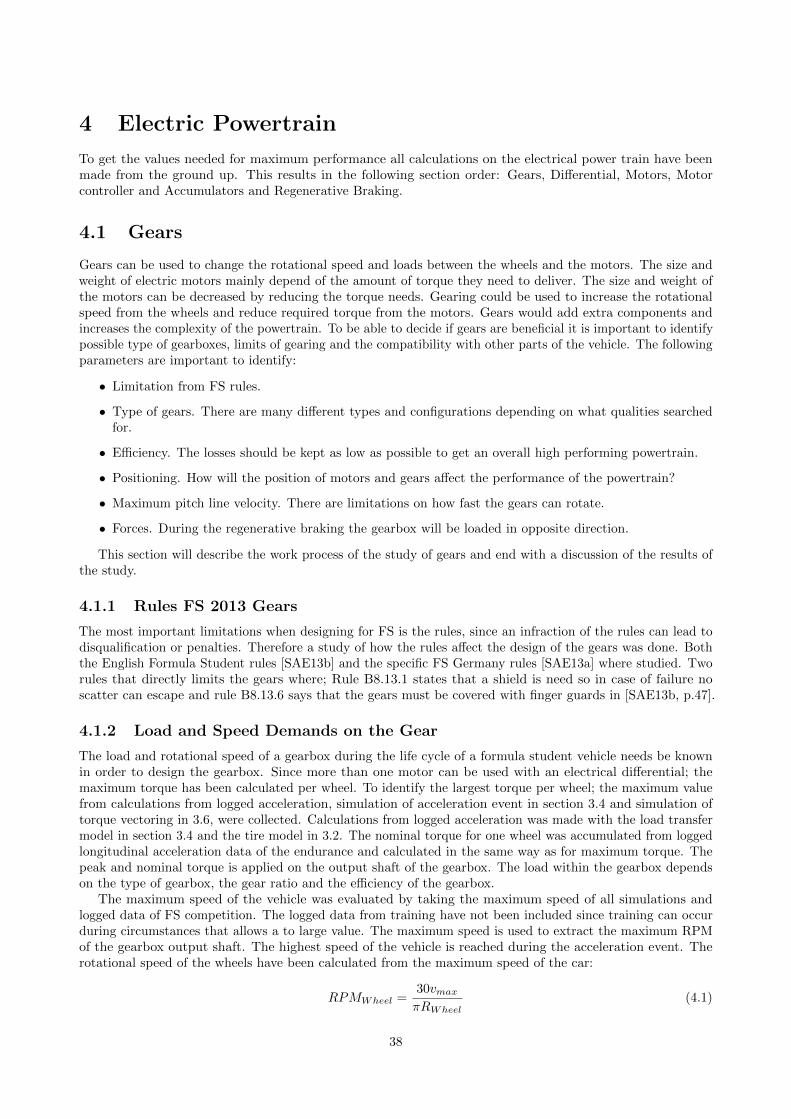
4 Electric Powertrain

To get the values needed for maximum performance all calculations on the electrical power train have beenmade from the ground up. This results in the following section order: Gears, Differential, Motors, Motorcontroller and Accumulators and Regenerative Braking.

4.1 Gears

Gears can be used to change the rotational speed and loads between the wheels and the motors. The size andweight of electric motors mainly depend of the amount of torque they need to deliver. The size and weight ofthe motors can be decreased by reducing the torque needs. Gearing could be used to increase the rotationalspeed from the wheels and reduce required torque from the motors. Gears would add extra components andincreases the complexity of the powertrain. To be able to decide if gears are beneficial it is important to identifypossible type of gearboxes, limits of gearing and the compatibility with other parts of the vehicle. The followingparameters are important to identify:

• Limitation from FS rules.

• Type of gears. There are many different types and configurations depending on what qualities searchedfor.

• Efficiency. The losses should be kept as low as possible to get an overall high performing powertrain.

• Positioning. How will the position of motors and gears affect the performance of the powertrain?

• Maximum pitch line velocity. There are limitations on how fast the gears can rotate.

• Forces. During the regenerative braking the gearbox will be loaded in opposite direction.

This section will describe the work process of the study of gears and end with a discussion of the results ofthe study.

4.1.1 Rules FS 2013 Gears

The most important limitations when designing for FS is the rules, since an infraction of the rules can lead todisqualification or penalties. Therefore a study of how the rules affect the design of the gears was done. Boththe English Formula Student rules [SAE13b] and the specific FS Germany rules [SAE13a] where studied. Tworules that directly limits the gears where; Rule B8.13.1 states that a shield is need so in case of failure noscatter can escape and rule B8.13.6 says that the gears must be covered with finger guards in [SAE13b, p.47].

4.1.2 Load and Speed Demands on the Gear

The load and rotational speed of a gearbox during the life cycle of a formula student vehicle needs be knownin order to design the gearbox. Since more than one motor can be used with an electrical differential; themaximum torque has been calculated per wheel. To identify the largest torque per wheel; the maximum valuefrom calculations from logged acceleration, simulation of acceleration event in section 3.4 and simulation oftorque vectoring in 3.6, were collected. Calculations from logged acceleration was made with the load transfermodel in section 3.4 and the tire model in 3.2. The nominal torque for one wheel was accumulated from loggedlongitudinal acceleration data of the endurance and calculated in the same way as for maximum torque. Thepeak and nominal torque is applied on the output shaft of the gearbox. The load within the gearbox dependson the type of gearbox, the gear ratio and the efficiency of the gearbox.

The maximum speed of the vehicle was evaluated by taking the maximum speed of all simulations andlogged data of FS competition. The logged data from training have not been included since training can occurduring circumstances that allows a to large value. The maximum speed is used to extract the maximum RPMof the gearbox output shaft. The highest speed of the vehicle is reached during the acceleration event. Therotational speed of the wheels have been calculated from the maximum speed of the car:

RPMWheel =30vmax

πRWheel(4.1)

38

The maximum speed of the car, ωWheels in relation to the maximum speed of the motor, ωMotor, willdetermine the ratio needed in the gearbox.

α =ωmotor

ωWheels(4.2)

4.1.3 Single or Multiple Gear Transmission

Unlike combustion engines, electric motors can produce high torque at low rotational speed. Electric motorsgenerally have a wider range where it can deliver maximum torque compared to combustion engines. The mainpurpose of the gears is to adapt motor torque to the demands of the powertrain. In a combustion engine avariable gearbox is use to adapt the motor torque characteristics to the demands of the powertrain. If thetorque characteristics of the motors fit the demand of the powertrain as with a PMSM chosen in section 4.3.4only a static gearbox is required. A static gearbox is less complex and smaller by size than a variable gearboxand will therefore be used.

4.1.4 Position of the Gearbox

The design of a gearbox is limited by its position in the vehicle since the surroundings have a major impact onthe gearbox. A study to identify possible positions of a gearbox in a FS car was made. The study includespowertrains utilized by competing FS teams as well as other powertrains on the market.

4.1.5 Different Types of Gears

To identify what kind of static gearboxes that can be used in the electric system, a comparison of differentgears have been made. Interesting parameter for each gear is the efficiency, weight, maximum and minimumgear ratio and if the gearbox can transport reversed power transport.

From simulation of the acceleration event simulated in section 3.4 the efficiency of the powertrain has a majorimpact of the performance. During the endurance event high efficiency of the powertrain is wanted. Thereforea high efficiency of the gears is wanted and gear with lower efficiency than 80% will not be investigated.

Maximum gear ratio is interesting since a high gear ratio will reduce the size of the motors. The minimalgear ratio of a gearbox is also of interest since the highest rotational speed of the output shaft is known. If thegearbox ratio is too high the motors will not be able to match the rotational speed of the output shaft duringmaximum speed and will break. Therefore has a minimal gear ratio been calculated. A fabricated PMSM havea normal range of 5000 to 15000 RPM. The highest RMP during FS2012 is 20000 RPM in the Delft vehicle.To completely include all possible motors a maximum RPM of 40000 RPM where used when calculated themaximum gear ration. With equation 4.2 the maximal gear ratio that will be investigated will be 1:30. Gearsas harmonic drive have then not been investigated further since there minimal gear ratio is 1:30.

When using regenerative braking the torque reverses direction and the gearbox have to be able to transferreversed load. Gear that cannot transfer reversed load will not be investigated. Gears that can transfer reversedload have been investigated so that they don’t self-locks i. e. the power losses is larger than the incomingpower. Self-locking can only occur when the rotational speed increases with the load transfer. With a reversingload the backslash of a gearbox have a major importance; since a large backslash would increase the load onthe teeth each time the load reverses direction. The backlash is measured different between resellers but ageneral comparison in backslash between types of gears is possible to do.

Ordinary Single Row Planetary Gears

Planetary gears have compact size and low weight per torque. This is because of its geometry that makesthree or four gear teeth in contact during load transfer so the load on the teeth is reduced three or four times.Planetary gears have three ways to transfer load, with the sun gear g1, the planetary gears holder gc or thering gear g2. Only single row planetary gear with locked ring gear will be studied; since this set-up is capableof giving the greatest range of gear ratio. A planetary gear of this set-up transport power axially. Since thegearbox will be used to gear down the torque from the motors to the ground a planetary gear with lockedring gear will have the following load transfer; the output shaft from the motor will be connected to the sungear and transfer the load to the planetary gear. The ring gear will force the planetary gear to rotate in thereversed rotational direction of the sun gear. The Planet carrier will transport the load to the output shaft of

39

Sun Gear, g1

Planetary Gear, gc

Planetary Gear, gc Planetary Gear, gc

Ring gear g2

ωc

ω1

ω2

Figure 4.1: Schematic illustration of ordinary Single row planetary gear

the gearbox. The relation between the rotational speed of the inner gears is shown in equation 4.3. In therange of 3-8:1 in gear ratio the efficiency with a locked outer gear is about 96-98% at maximum load [Gro09].A simplified way to calculate gear ratio and efficiency is shown in equation 4.3 to 4.9. It do not take anyprecautions of mounting conditions but gives a hint of how a gearbox would behave. The rotation between thegears in a planetary gears is shown in equation 4.3 where zi is the number of teeth and ωi rotational speed oncorresponding gear gi.

−z2z1

=ω1 − ωc

ω2 + ωcR = −z2

z1(4.3)

The transferred load with the ring gear locked is shown in equation 4.4.

ω1 − ωc

0 + ωc= R→ ω1 = (1−R)ωc (4.4)

Equation 4.3 would produce the gear ratio of a transmission with sun gear as input and planet carrier asoutput.

ωc(1 +z2z1

) = ω1 ⇒ α = 1 +z2z1

(4.5)

Efficiency losses in planetary gears is bearing losses, lubrication losses and gearing losses. Only the gearinglosses will be studied for now since they are most likely to be the largest. The efficiency of the gearing dependsof what kind of gears you are using inside the planetary gear, spur gears is the most common since they do notadd any extra axial forces and have the greatest efficiency. Since the load passes two gearings the efficiencyof the gearbox can be approximated by adding the efficiency of those two gearings [Fer83]. The standardcalculation of efficiency used in [MM09] approximate the efficiency between the ring gear to the planetary gearand planetary gears to sun gear be the same. This limits the calculation of the efficiency and has not beenused. The power losses in a planetary gears is described in equation 4.6.

Pf = η1 | (ω2 − ωc)T2 | +η2 | (ω1 − ωc)T1 | (4.6)

40

The rolling condition from equation 4.5 combined with 4.6 gives the power losses with a locked ring gear.

Pf =(η1 + η2)αTcωc

1 + α(4.7)

The efficiency will then be the power out, divided by the power in 4.8.

η =Pin − Pf

Pin=

1 + (η1 + η2)α

1 + α(4.8)

Self-locking only occur when gearing is increasing the speed and not when gearing reduces the speed.Self-locking could occur with a three staged gearbox if the load travels from planet carriers to the sun gear. Theradius of the sun gear and the ring gear must then be close to each other which is a very low gear ratio singlerow planetary gear and is unlikely to be used. With a four geared epicycle gearbox, a self-locking constructionhappens easy at higher gear ratios [MM09] .

Backlash can be reduced by high precision manufacturing and reducing the size of the teeth.By row mount multiplied planetary gears greater transmission rates can be a acquired but the efficiency is

lower by each extra row se 4.9.

αnew = α1 × α2 × ...× αn ηnew = η1 × η2 × ...× ηn (4.9)

The major disadvantage of planetary gears is that it’s difficult to design and construct since great precisionis required to keep the efficiency high and backlash low and the limited gear ratio.

Spur Gears

Spur gears are the simplest type of gear with straight cut teeth aligned parallel to the axis of rotation. Spurgears have high efficiency in comparison with other gear types. Since the entire face of the teeth engages atonce, spur gears are noisy at higher speeds. This should not cause any problem in race car applications though.The ratio should be kept below 5-6:1 to avoid increased size and lowered strength. If the ratio needed exceedsthis limit, a two-step gearbox will be required. This implicates increased weight and lowered efficiency.

The range of efficiency is 97-99.5 % for the spur gear depending on the size and rotational speed. Thisvalue is for one-step, if more than one step is used, the efficiencies will be multiplied. As mentioned before thereduction ratio should be kept below 5-6:1 but an internal design is possible were the range of reduction is5-7:1. The max pitch line velocity should not be higher than 20-25 m/s. [Rad12].

Helical/Double Helical Gears

The helical gear has angled teeth instead of straight-cut. This means that the teeth engage gradually, causingthem to run more smoothly and quiet. They can also be used in high speed applications that are when thepitch line velocity exceeds 25 m/s. The angled teeth causes a resultant thrust along the axis of the gear whichhas to be accommodated by bearings. To overcome this problem one can use double helical gears, having twosets of teeth in a V-shape cancelling the axial thrust. The big disadvantage in race car applications is the lossof efficiency in comparison with the spur gears [Rad12].

Chain Drive

Chain drive makes it possible to transmit power over longer distances then spur gears. Previous CFS cars withcombustion engines have had chain drive because the distance between the chassis mounted motor and thedriving shaft. Electrical motors could be mounted close to the driving shaft, making it possible to use directgears such as those mentioned earlier. The chain drive have lower efficiency compared to spur- and planetarygears [Scl07]. A Chain drive drastic drops in efficiency at higher rotational speed which most likely will bereached [BL04].

Belt Drive

Belt drive have the same advantages as the chain drive making it possible to transmit power over distances,but is less efficient than chain drives [Scl07].

41

Continuously Variable Transmission

Continuously variable transmission can change the gear ratio seamlessly. This is normally used to keep themotor at its optimal speed and thereby its best efficiency. The disadvantages are the high mass and lowefficiency making them inappropriate in race car applications.

4.1.6 Results and Discussion

The results from the models will be presented and discussion on gear types and configuration will follow.

4.1.7 Loads

The maximum load during all events is 459Nm and occurs during the 4WD simulation of the accelerationevent. This is the maximum load on one wheel and what the output shaft of a gearbox needs to be able totransport during peak load. The safety degree i. e. how much the gearbox is designed to withstand comparedto the maximum load have not been decided and only the maximum load is presented. Fatigue calculationshave not been made and the nominal torque is only of interest during those calculations for the gearbox. Thenominal torque during the endurance and autocross event is Nm. The limitations and simplification of thedata from the simulation of the 4WD acceleration event reduce the readability of the data. The rateability ofthe data itself is discussed in the section 3.4.

4.1.8 Gear Ratio

The weight of the motor can be reduced by increasing the gear ratio and having the motor working at higherspeed. This would in most cases lower the gearbox efficiency since higher gearing ratios or use of two stagesnormally increase the losses. A increased gear ratio in the same kind of gearbox will generally increase thesize of the gearbox. From the maximum resumed speed of 131km/h which occurs during the simulated 4WDacceleration event the RPM of the output shaft is known. With combination of the maximum motor RPM agear ratio can be calculated by equation 4.2. Since the maximum RPM of the motor is unknown the gear ratiocan not be calculated. A iteration between the motors maximum RPM and required torque will be neededlater.

4.1.9 Position of Motor and Gearbox

The choice of gear type and configurations is dependent of the position of the gears and motors. Two differentstrategies in the placement of motors and gears were decided from the study of gear position; Either in thewheels, or in the chassis.

In Wheel Mounted

In wheel mounted motors have a limited volume because of the surrounding rim and the nearby suspension.From the vertical dynamics 3.3 the importance of weight is larger than in other parts of the vehicle and thereforetorque to weight ratio have a larger impact. The gearbox with the best torque to weight ratio is the planetarygear. The possible volume of in wheel mounted motors also coincidence with the shape of a planetary gearbox.With planetary gear the ring gear can be used as the base for the wheelhub and used for attachment for thesuspension. Planetary gears have a maximum recommended gear ratio of 1:8 and if a larger gear ratio is needed,the efficiency will be reduced or a second stage would be needed. A higher gear ratio than 1:8 is likely so thatthe size of the motors will be reduced. A problem with wheel mounted motors is that the components are morespread out. This means that power and water cooling needs to be transferred a longer way compared with achassis mounted motor.

Chassis Mounted

If the motors are placed in the chassis, space is not as limiting as in-wheel mounted system. Therefore eitherspur gears or planetary gears can be used. A chassis mounted motor got the disadvantage that it needs totransmit its power from the chassis to the wheels. An in-chassis motor almost always needs to be water cooledsince the air flow is not enough to cool the motors. The great advantage of a chassis mounted motor is that

42

the weight and size of the motors can be made bigger and therefore a lower gear ratio can be used. This willreduce the demands of the gearbox.

4.2 Differential

The differential is a device that allows the inner and outer wheel to rotate at different speeds when cornering,where the outer wheel follows a longer path and needs to rotate faster. Since electrical motors will be used inthe FS car, an electrical differential can be implemented. Another way to transport power to the wheels is touse a mechanical differential. Following parameters are important when designing a differential:

• Efficiency. The overall powertrain efficiency is to be kept as high as possible, therefore losses in theincluded components has to be minimized.

• Weight. Lower weight will increase the performance of the car.

• Under what conditions is it possible to implement an electrical/mechanical differential and what are theadvantages?

4.2.1 Mechanical Differential

The mechanical differential uses gears to transmit torque and rotation, usually from one input shaft to twooutput shafts, which are allowed to rotate in different speeds. If the input speed is held constant and the speedof one of the outputs is increased, the other will decrease. The two most common mechanical differentials arebevel gear differential and spur gear differential. The bevel gear differential is the mechanical differential thatis implemented in the most cars. The spur gear differential is a more lightweight planetary differential. Thistechnique is new and will probably be more common in the future. The planetary differential is 34% lighterand 73% smaller than a bevel gear differential [RSHM11]. Because of the superior weight and size the planetarydifferential is a better choice for a formula student car. Another technology is the electronically controlleddifferential, so called active differential. This could adjust the torque distribution between the inner and outerwheel, using an electronic control unit. This makes it possible to implement torque vectoring on a mechanicaldifferential.

4.2.2 Electrical Differential

To use electrical differential, there have to be two independent motors for every driving wheel-pair. Theelectrical differential has the advantage that power and torque could be applied independently on the differentwheels. When cornering, power must not be taken from the inner wheel to apply more power on the outsidewheels. The electrical differential also makes it simpler to implement a torque vectoring system.

4.2.3 Conclusions on Differential

If there will be only one motor in the car, a mechanical differential has to be used. The mechanical differentialwill add weight and losses to the system. In the case where one motor is used and torque vectoring should beimplemented, an active differential have to be used. The controlling of the active differential will add complexityto the system. If there will be more than one motor, i.e. one motor for every driving wheel, an electricaldifferential could be implemented and will be the best solution. The weight will be lower when no mechanicaldifferential is needed but this may be compensated for the weight of the extra motors. No mechanical gearshave to be used that add weight and losses to the system. Torque vectoring will be, as mentioned before,simpler to implement.

4.3 Motors

During the dynamic event of Formula student the powertrain should be able to deliver the torque that thevehicle can transfer to the ground. An overcapacity would only lead to extra weight and under-capacity wouldlead to lower performance. The aim is then to choose a motor that would best fit the needs for the CFS14EV.To do this, the demands and limits of the motors must be identified. Following parameters are important whenchoosing and designing the motors:

43

• Rated power. This is the mean power that the motors are designed to handle without overheating. Undershorter time it is no problem to exceed this power. It should also be noted that the regenerative brakingwill also load the motor and therefore will be taken into account when calculating the rated power. It iseither the Endurance event or the Autocross event giving the highest requirements.

• Maximum torque. The motor will be designed so that they are able to give the torque that the tractionto the road is allowing. This is calculated from maximum longitudinal acceleration, see section 3.4. Whenbraking, the braking torque must not only be applied from the motors, but also the mechanical brakes ifnecessary.

• Maximum speed. This will determine the gear ratio needed, if needed at all.

• Limits by the FS rules.

• Motor type. Different motor types have different characteristics, a comparison will be done in section 4.3.2.

• Efficiency. High efficiency is a high priority since this is part of the competition.

• Distribution between front and rear motor power. Together they should be able to give 85 kW, but dueto load transfer more traction is available on the back wheels during acceleration.

The motors main connection and limits are.

• Combination with gearbox.

• Powering system and motor controller.

• Other nearby objects like suspension and chassis that will state geometric constraints.

4.3.1 Rules

There is a large amount of rules for schedules of emergency stops and protection of the motors but few thatlimits the motor itself. Rules for protection of the driver will limit the positions where the motors can be placedi.e. rule EV4.2.2 in [SAE13b] any part of the tractive system need to be protected for rear and side collisionswith a triangulated structure of metal pipes. This would make it impossible to have the motors at the outerend of the car. Only plain water or plain oil may be used for cooling the motors.

4.3.2 Different Motor Types

A general comparison of different motor families has been done. The motors will be compared and investigatedby the efficiency, torque to weight ratio/volume and complexity. The characteristics of the torque, maintenanceof the motors and reliability will also be investigated.

PMSM/BLDC(brushless DC) Motor

The characteristics for the PMSM is high torque per weight, torque per volume and high efficiency [Hug20]which makes it ideal for a racing car. The controller for the PMSM is more complex than for a DC poweredmotor. The motor delivers rated torque up to the rated speed. Beyond the rated speed, the motor operates ina constant power mode where torque falls off at a rate that is inversely proportional to the speed, it is calledfield weakening. In most cases the maximum speed of the motor is considered to be at the end of the constantpower region. PMSM is possible to map the efficiency by variate the positions of the permanent magnets andchanging the number of poles as simulated in [FHH10].

Brushed DC Motors

There is a variation of Brushed DC with different torque characteristics and efficiency. The common for all DCmotor is that they are not maintenance free and by using the motor the brushed wears down and performancechanges. Brushed DC motors do not have as high peak torque per kilo as a PMSM. The motor controller tothe Brushed DC motor is simpler than motor controllers for PMSM or asynchronous motors.

44

Induction/Asynchronous Motor

The induction motor is mostly used when weight isn’t a problem because of lower torque per weight ratio,compared with PMSM, or when a steady speed is required since it is very speed stable. The efficiency variesroughly from 87 to 97% depending on the speed and load.

Hub Motor

A hub motor would not require a gearbox which would make the design less complex, but the torque to weightratio will probably be little smaller than a in wheel motor with gearbox [Bru+12]. The problem with the hubmotor is the increase in the rotating mass since a large magnet is rotating. This would by the law conservationof angular momentum increase the loads of the suspension holders when steering and would make it harder tosteer. This is just an assumption and no calculations have been made.

4.3.3 The Load Characteristics of the Motors

The loads of the dynamic event were acquired from simulations and logged data, much in the same way asfor gears. This data will be used for the calculations of peak and nominal torque, nominal and peak effect inthe same way as in gears. The torque will be calculated as with no gear box since the characteristics of thetorque is the most interesting. The same data as in gears have been used but combined with the speed so thatthe torque demand can be combined with the appropriate RPM. Logged deceleration was used to be able tocalculate the demands of the motors in reversed direction.

4.3.4 Results and Discussion

The results will be presented and discussed individually. The torque calculations have been done with thecalculations from the models in section 3.

Motor Type

The motor type that has the best performance by weight and highest efficiency is the PMSM. A PMSM have ahigh torque per weight with a long span where it can deliver this peak torque. A DC-motor have a lower peaktorque per weight compared to PMSM and have a smaller ranger where it can deliver the torque. Asynchronousmotor have to low torque per weight and is built to be held at a constant rotational speed. The Torquecharacteristics of the motor will also match the demands of the torque demand of the powertrain as shown insection 4.3.4.

Peak Torque From Simulations

From simulation of the acceleration event the characteristics of the maximum torque possible to deliver tothe ground without spinning was accumulated.The maximum possible torque increases from still standingas a consequence of the increased down force by the aero-package and then rapidly loses torque since themaximum allowed power consumption at 85Kw is reached. To optimize the capacity of the motors the torquecharacteristics of the powertrain should match the maximum torque delivery possibilities as much as possible.This characteristic can be achieved either with a multi staged geared gearbox as in petrol driven FS cars orwith an electric motor of the same characteristics of the delivery demands with or without a static gearbox.

In a PMSM the torque is near constant until it reaches its nominal speed. Then the motor controller willhold the power constant and increase the speed of the motor which will make the torque decrease, this is calledfield weakening. Both the motors and the CFS car are limited by their maximum power consumption anddecrease the torque to hold constant power consumption as speed increases. Therefore the torque characteristicof the motors and power limits is similar to each other. To optimize the motors size the motors should not beable to deliver any more torque when the tire slips or when the power limit kicks in. From this and that thetorque characteristics of a PMSM the nominal RPM of the motors should be configured so that it occurs nearwhere the maximum power delivery is reached. The peak torque of the motors could be designed either by themaximum torque in the event or the start torque.

If the motors is designed for a torque curve as the one in figure 4.3a the area between the red and bluelines are extra power never going to be used. If the motors is designed as the curve in figure 4.3b the areabetween the red and blue lines are missed and unused potential possible torque, the reduced torque will increase

45

0 0.5 1 1.5 2 2.5 3 3.5 40

200

400

600

800

1000

1200

[sec]

[Nm

]

Torque56km/h

(a) 4WD

0 0.5 1 1.5 2 2.5 3 3.5 40

200

400

600

800

1000

1200

[sec][N

m]

Torque56km/h

(b) RWD

Figure 4.2: Maximum Torque Distribution during maximum Acceleration

the range of where maximum torque could deliver but the speed during the acceleration event. The latteralternative would reduce the acceleration of the car but would even out the acceleration during acceleration.The overcapacity would keep reduce the risk of motors overheating but would do the motors heavier.

(a) Highest torque (b) Start torque

Figure 4.3: Different kind of configureation

RWD Peak Torque

During the acceleration the demands of the powertrain coincidence with the demand of torque delivery of therear shaft. The characteristics of the motors powering the rear shaft therefore needs to be configured to applyfigure 4.2b. The demands of a torque vectoring system would increase the peak demands of the motors but theload characteristics during acceleration would be very much alike. Deceleration during regenerative brakingwould not load a RWD system noticeable compared with the acceleration and have therefore no impact on the

46

design of the motors.

4WD Peak Torque

During acceleration the car squats and the weight distribution moves backwards on the CFS. The weightdistribution of the car at the maximum acceleration of is 81 % on the back and 19 % the front wheel pair. Bythis during the acceleration the front motors needs to deliver a smaller amount of torque than the back motor.The reduced acceleration at the power limit the weight distribution evens out. This change the characteristicsof the load of the motors, the rear motors will decrease faster in delivery needs and the front shaft torqueincreases due to the change of weight distribution compared to normal field weakening. The load characteristicsduring maximum acceleration of the front and back motor are illustrated in figure. This particular weightdistribution only occurs during maximum acceleration on a straight line, in cornering the load transfers inlateral directions and the distribution will shift between left and right wheels. During simulation of torquevectoring 447 Nm was the maximum torque per wheel. The maximum torque from the longitudinal model is459 Nm.

0 0.5 1 1.5 2 2.5 3 3.5 450

100

150

200

250

300

[sec]

[W]

FrontBack

Figure 4.4: 4WD Torque Demands of the front and rear wheel pair during maximum Acceleration

During deceleration the car sits and the weight distribution moves to the fort wheel pair From logged dataevents of CFS12 the peak deceleration measured is 1.6 g. The weight distribution shifts to 78% in front and22% in rear. Around 78% of braking energy needs to be accumulated in the front shaft during peak braking.To be able to accumulate as much power as possible with regenerative braking both front and back motorsneeds apply the reversed maximum torque on the back and front wheel. The torque needed on the front shaftduring maximum deceleration is 842Nm. The approximated value per motor is 421Nm per wheel but due tocornering these values shifts.

To fully apply the torque needed both in delivery and accumulated the front shaft needs to be ableto accumulate 842Nm and the rear shaft deliver 919Nm. The difference between acceleration torque anddeceleration torque is because the CoG is 54 % to the rear and the aero and rolling resistance. The greatdifference between the front and rear shaft during high longitudinal acceleration and deceleration makes that aovercapacity of motor power needs to be built in if all torque is going to be accumulated. During the accelerationthe front motors have an overcapacity and during the deceleration the rear motors have an overcapacity. Areduced motor capacity on the front shaft will reduce the amount of possible regenerative power.

47

4.3.5 Nominal Torque

2WD

The nominal Torque needed using 2WD is 429 Nm. The nominal torque has been calculated by the RMS valueof Torque demands during endurance and sprint event. Only positive acceleration in longitudinal direction hasbeen measured since even if regenerative braking is used, the loads of the rear shaft are low compared to theloads during acceleration.

4WD

Sprint and endurance, both the forward and reversed torque divided between the motor pairs with accelerationdata and load transfer model.

4.3.6 Motor Nominal-RPM and Maximum-RPM

To minimise the weight and size of the electric motors they should have as high RPM as possible as the gearscan handle efficiently. With a higher RPM a smaller torque would be needed and therefore smaller currents inthe winding. The relation between nominal and maximum RPM is decided by the demands of the powertrainand is illustrated in figure 4.4. The nominal-RPM should occur right after the maximum power consumptionoccur so that the motors will not be limiting. The nominal RPM for a 4WD system should occur at 60km/mand at 80km/h for a RWD system. The later nominal RPM for the RWD is because the delayed reach of powerconsumption limit. The maximum RPM for both simulations is 131km/h. And from maximum logged datafrom the endurance event the max speed is 95km/h.

4.3.7 Motor Efficiency

The efficiency of the motors needs to be optimised where it is needed most. During the endurance, points aregiven for a more efficient system and the limit of 85kw makes efficiency important. The motors should then bemost efficient in the range of the endurance event and where the maximum power consumption occurs. Theaverage speed of the endurance event last year were 59.574km/h where speed distribution is right skewed. Theefficiency of the motors during the endurance event therefore needs to be around the mean speed or lower. Themean torque of the endurance event is 37% of max torque, therefore around these two values the motors needto be configured.

PMSM can be configured to have different efficiency mapping. The mapping of a PMSM is normally notpresented from manufactures but a theoretical simulation of efficiency and delivery capabilities have be madeby [FHH10]. This papers simulation make us recommended a VI-PMSM since it highest efficiency is before andduring the nominal and maximum torque which match the demand of the motor efficiency. The weight of anefficient system at this point is simulated and shows that a high efficiency during acceleration near maximumpower consumption, a 5% efficiency loss in this position will reduce the Acceleration event with 0.2 seconds.

4.3.8 Cooling

The amount of cooling needed for the motors depends of what degree of efficiency and power consumption. Ahigh power consumption combined with low efficiency would drastic increase the required cooling.

4.3.9 Discussion

The high efficiency and low weight of the PMSM makes it a certain pick. The characteristics of the torquedelivery from a PMSM are matching with the demands of the powertrain very neatly. The efficiency can bemapped to match the optimal efficiency map of the car.

A smaller front motor will directly decrease the possible amount of energy that can be used for regenerativebraking. The cooling system of a PMSM would preferably be a water cooled system. This is because it wouldreduce the size of the motor and that an already existing cooling system exist that might be possible to use.

The greatest limitation of the gearbox is the maximum RPM, limited by either the gearbox or by the motor;this will set the minimum possible size of the motor.

The demands of a regenerative system with a 4WD makes the demands of the front motors variate greatly,furthermore the size of the motors needs to be done with concern of amount of lost possible regenerative energy.

48

From accelerating perspective the motors of the front should be small to reduce the weight and extra loads onthe front suspension.

The efficiency map of a VI-PMSM is the motor that best fits the demand of the events.

4.4 Motor Controller

The motor controller controls the speed and torque of the electric motors. The demand from the motor decidesthe demands of the motor controller. Therefore since a PMSM is the most preferred motor shown i section 4.3the controller will need to be able to deliver current controlled power and adapted to the wanted frequencywith the motor. The controlling of a PMSM is complex but the important design parameters are:

• Maximum voltage.

• Maximum current.

• Need for cooling. Probably the hardware needs to be water-cooled due to high terminal losses becausethe high currents.

• Support for regenerative braking.

4.4.1 Master Controller

The master controller handles the signal from the driver, via pedals and steering wheel, to the motor controllers.If torque vectoring is implemented, the master controller will do the calculations. The unit should be dimensionedto fit more applications than needed today, so the possibility for more implementations will be available forfuture work. This unit could also control the power output so it doesn’t exceed the limits set by the rules.Some signals are displayed in table 4.1 and a block schematic is shown in figure 4.5. This is an example ofsignals and will probably be increased over time.

Table 4.1: Master controller signals.

signal signal type commenttorque input from acceleration pedalbrake input from brake pedalsteering wheel angle input to define where the driver want to gowheel speed input signals from the wheels for traction control, ABS and estimating speed of the cartemperature input to protect motors, batteries and electronicstorque output torque request to the motor controller Xestimated speed output estimated longitudinal speed

49

Master controller

Motor controller LR Motor controller RR

Motor controller LF Motor controller RF

Motor LF Motor RF

Motor LR Motor RR

steering wheel angle

wheel speed

torque torque

torque torque

A,B,C HA,HB,HC A,B,C HA,HB,HC

A,B,C HA,HB,HC HA,HB,HCA,B,C

temperature

brakeestimated speed

torque

Figure 4.5: Master controller block schematic.

50

4.5 Accumulators and Regenerative Braking

When using mechanical brakes such as disc or drum brakes, kinetic energy is transformed into thermal energy.The idea of regenerative braking is to store and reuse this energy. This lowers the capacity demands on theaccumulator pack i.e. making it lighter. Regenerating lost energy also results in an environmental gain which isrewarded with points in the efficiency event. These two factors make regenerative braking very interesting for aFS car.

4.5.1 Types of regenerative braking

There are many ways to regenerate the lost energy. The most common techniques that have been successfullyimplemented in race cars are mentioned below.

Mechanical- Flywheel

When the car brakes the idea is to transform the kinetic energy, shown in equation 4.10, into rotational energyin a flywheel, described in equation 4.11. When the car is braking the flywheel is connected to the driveshaft with a clutch and accelerates due to the braking momentum, shown in equation 4.12. When the car hasreached the desired speed the flywheel is disconnected from the drive shaft. To reuse the energy, the flywheel isreconnected to the drive shaft and energy stored in the flywheel is redirected into the car. This would howeverrequire new components to be assembled to the car i.e. extra weight and more moving parts. This method iseffective under the right circumstances - high vacuum and magnetic bearings. This results in a efficiency of 97%.Iz is the moment of inertia, which is defined as the resistance to an angular change around an axis. A large Izmeans that a lot of energy could be saved in the flywheel. The moment of inertia of a thick cylinder, which isa good approximation for flywheels is described in equation 4.13. The construction is therefore complex toimplement. The energy possible to store in a flywheel depends on the mass and the radius of the wheel.

Ek =1

2mcv

2 (4.10)

Ef =Izω

2

2(4.11)

Mb = Izω (4.12)

Iz =1

2m(r21 + r22) (4.13)

Where:Ek = kinetic energy of the carv = velocity of the carmc = mass of the carEf = energy of the rotating flywheelm = mass of the rotating cylinderr1 = outer radius of the flywheelr2 = inner radius of the flywheelIz = moment of inertiaω = angular velocityω = angular accelerationMb = braking momentum

The flywheel must be able to store the kinetic energy of the car driving at full speed to maximise the effectof the regeneration. The maximum speed is designed to 130 km/h and the kinetic energy is at this speed about0.05 kWh. A formula student car is light weight which makes this possible with a small and light flywheel. Aflywheel is hard to implement in a car with many motors because all the motors need an individual flywheel. Itis also harder to implement with in wheel mounted motors because of the lack of space in the rim. A flywheelis therefore most effective in a RWD car with one motor and one shaft connecting both rear wheels.

51

Electrical - Alternator

The kinetic energy is transformed into electric energy via alternator. This is done by phase shifting the currentto the motor. When the car is moving and the phase is shifted, a current is induced in the motor. Theinduced current then recharges the accumulator pack consisting of either batteries, capacitors or both. Thismeans that the kinetic energy is converted into electric energy which is easily reused. Electrical regenerationwith alternators is easier to implement with multiple motors than a mechanical flywheel since the motor andalternator is the same component.

Super capacitors

A super capacitor works in this application as energy storage. Super capacitors works as an ordinary capacitorand the prefix super tells that the capacitor have a high capacity. The energy is charged in an electric fieldbetween two conducting plates. Super capacitors generally have higher specific power (W/kg) and lower specificenergy (Wh/kg) than a battery. In a car, super capacitors are mainly used to increase efficiency when combinedwith regenerative braking. The reason for this is that super capacitors have a lower inner resistance andtherefore have less heat losses. Super capacitors also have a slightly higher temperature work range thanlithium-ion batteries, which make them more robust. Equation 4.14 describes how much energy that is storedin the capacitor.

Ecap =CV 2

2(4.14)

Where: C = capacitanceV = voltage over the capacitor

Because of the limitations in the rules regarding a maximum voltage of 600 V over the accumulator packthe capacitance needs to be high enough to make sure the braking energy can be regenerated without exceedingthe limiting voltage.

4.5.2 Method

To simplify the problem of designing an accumulator pack the problem was initially divided into three differentareas. When all of the demands were met the main focus was to make the accumulators as light weight andenergy efficient as possible.

• The accumulator needs to be able to release a large enough power burst for the acceleration event. Thisgoal is set in relation to the acceleration event since this event sets the highest demands on accumulatorsin terms of large amounts of energy released in short periods of time.

• The accumulator needs to be able to hold enough energy to complete an endurance event. Endurance isby far the longest event; therefore it sets the highest demands on the power capacity of the accumulators.

• Another important factor for the battery pack is the heating problem. Whenever the accumulators releaseenergy or is being loaded energy is lost due to inner resistance. This energy is turned into heat. This is aproblem since a accumulator is easily damaged if the temperature rises above 60oC.

By analysing the endurance lap from Silverstone 2012 the energy requirement was calculated. Using thelogged acceleration and velocity a model was set up to calculate the power drawn out from the battery pack.Only the longitudinal acceleration is possible to regenerate. The model is simplified since it assumes constantroll resistance, drag force with constant drag coefficient, and an approximated total efficiency of the car. Inequation 4.15 the Heaviside function, H(ai), makes sure no energy is regenerated while braking. There are FSrules that states that in different circumstances the mechanical brakes must be used. The factor (ηreg = 0.8approximates this behaviour [Int], the last 20 % of the energy is transformed into thermal energy in themechanical brakes.

Wbattery =1

η

n∑i=1

(maiH(ai) +cdρApV

2i

2+mgf)Vi∆t (4.15)

52

Where:Wbattery = battery capacityη = total efficiency of the carn = number of sampled datam = mass of the carai = logged accelerationH = Heaviside functioncd = drag coefficientρ = air densityAp = projected areaVi = logged velocity∆t = sample rate

This equation is in its simplest form and becomes more advanced when including regenerative braking.Then the equation takes the following form. In the equation it is approximated that the efficiency from thebattery pack to the tires is the same as from the tires to the battery.

Wbattery =

n∑i=1

(maiηH(ai) +maiηηreg(1−H(ai)) +

cdρAV2i

2η+mgf

η)Vi∆t (4.16)

Where:ηreg = regenerative factor

Batteries

A battery that is optimized can be either energy optimized or power optimized. An energy optimized battery isdesigned to deliver the required energy and the deliverable power is higher than the designed target. A poweroptimized battery has been designed to deliver the required power and will therefore have higher energy thanneeded. To create the optimal battery the battery needs to be designed to be both energy and power optimized.To do this, the optimal cell should have a certain ratio of specific energy over specific power. This is one of themain reasons why the battery should be designed especially for FS competitions. It is important to know thatthe, in data sheets given, specific power of battery cells is for continuous usage and not for peak power. Thevalue of the maximum peak power is much higher than the value for continuous usage. The specifications givenin data sheets are for long life service and can be exceeded. The C-number is a unit in the battery specificationthat tells how fast the battery can be discharged. The product of the discharge time in hours and the C-numberis set to 1. A C-number of 1 means that the energy can be discharged in 1 hour, a C-number of 2 means thatthe energy can be discharged in 30 minutes. Batteries also have a C-number for charging which works in thesame way.

Battery cell types

There are many different cell types. Important key factors when choosing a cell type for CFS are:

• Specific power, important for the acceleration and autocross events

• Specific energy, important for the endurance event

• Discharge rate (C)

• Charge rate (C)

• Safety

Battery model To set up a basic model for the battery is hard and to construct a well working batterypack, calculation software is needed. The calculation software is used to monitor the remaining energy and thetemperature in the battery during a simulated race.

53

Lithium-Polymer battery Li-Po cells are used for many different applications; from hand held devices tovehicles. The cells typically have a high specific energy; this allows the battery pack to be lighter. However,Li-Po batteries tend to have a low discharge rate but as long as the requirements from the acceleration eventare met Li-Po batteries are a good choice. When Li-Po batteries becomes overheated they can start to burn,this is a security risk. Therefore the FS rules require that 30 % of the cells have their temperature monitoredactively. Li-Po batteries have an efficiency of approximately 95%.

Lithium-Iron-Phosphate battery LiFePO4 cells usually have a lower specific energy than Li-Po. However,the discharge rate and specific power is higher. The cells have become popular in electric and hybrid vehiclesbecause of the high safety. When the LiFePO4 cells are overheated they can melt but it is impossible forthem to start to burn under normal conditions. Because of this, there is an exception in the rule about activetemperature monitoring. LiFePO4 batteries have an efficiency of approximately 95%.

Balancing system

Battery cells of the same type have variance in their properties, e.g. lower capacity than the specified in datasheets. To ensure a maintained performance of the batteries they must be connected to a balancing system.The balancing system makes sure the battery cells are evenly loaded. There are two types of balancing systems;active and passive systems. The active system actively measures how loaded each cell is and makes sure itis not overloaded. The system also measures the temperature of each cell, this is very important when usinge.g. Li-Po batteries. The passive system does not actively measure anything. A passive system loads each cellevenly. This means that might get unevenly loaded and some of them might be overloaded which can damagethe cells.

4.5.3 Cooling

Cooling is very important to consider for the car to be able to control the temperature of different components.If the components becomes too hot, they can be damaged and become a potential safety risk. The componentsthat need to be cooled are the accumulator pack, motors, gears, power electronics and the motor controllers.Since the different components have different maximum work temperature the cooling needs to be designed sothat the cooling reaches the demands for each component. There are two main types of cooling systems, aircooling and water/oil cooling.

Air cooling

In air cooling the flow of colder air over a hotter area is what drives the cooling. The air temperature isimpossible to control so the mass flow of air and the area that has air contact is what can be designed. Themass flow around different components is depending on the aerodynamics of the car. To get sufficient coolingthis can affect the drag and lift coefficients, decreasing the car’s aerodynamic performance.

The contact area can also be designed by using cooling fins. These are often used in electrical applicationsto reach sufficient cooling. The cooling fins also add extra weight to the car and might interfere with theaerodynamics.

Water/oil cooling

Water/oil cooling is more effective than air cooling. The reason for this is that water and oil have higher specificenergy and thermal conductivity than air. This makes the cooling more efficient than with air. What makesthis harder to implement in a car is that the hot water or oil must be air cooled. The water cooling systemaffects the car by adding weight and complexity. The pump is powered electrically which raises the capacityrequirements on the accumulators.

The maximum temperature for almost all lithium batteries is 60oC. Thus, the battery can absorb a highamount of energy that does not need to be cooled off. To have a high working temperature in the batteryalso help the cooling since the temperature difference between the battery and the air/water is what drivesthe cooling. It is important to know at what temperatures the car will be driven in to make sure the coolingsystem is designed properly.

If it is chosen that the motors should be water-cooled it might not be possible to water cool the batteries inthe same system. Since the different components have different working temperatures, the cooling systems

54

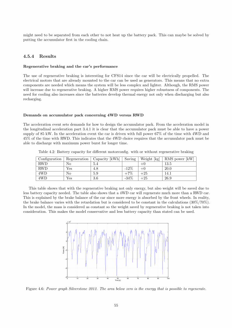
might need to be separated from each other to not heat up the battery pack. This can maybe be solved byputting the accumulator first in the cooling chain.

4.5.4 Results

Regenerative braking and the car’s performance

The use of regenerative braking is interesting for CFS14 since the car will be electrically propelled. Theelectrical motors that are already mounted to the car can be used as generators. This means that no extracomponents are needed which means the system will be less complex and lighter. Although, the RMS powerwill increase due to regenerative braking. A higher RMS power requires higher robustness of components. Theneed for cooling also increases since the batteries develop thermal energy not only when discharging but alsorecharging.

Demands on accumulator pack concerning 4WD versus RWD

The acceleration event sets demands for how to design the accumulator pack. From the acceleration model inthe longitudinal acceleration part 3.4.1 it is clear that the accumulator pack must be able to have a powersupply of 85 kW. In the acceleration event the car is driven with full power 67% of the time with 4WD and45% of the time with RWD. This indicates that the 4WD choice requires that the accumulator pack must beable to discharge with maximum power burst for longer time.

Table 4.2: Battery capacity for different motorconfig. with or without regenerative braking

Configuration Regeneration Capacity [kWh] Saving Weight [kg] RMS power [kW]RWD No 5.4 +0 13.5RWD Yes 4.8 -12% +0 20.04WD No 5.9 +7% +25 14.14WD Yes 3.6 -34% +25 26.9

This table shows that with the regenerative braking not only energy, but also weight will be saved due toless battery capacity needed. The table also shows that a 4WD car will regenerate much more than a RWD car.This is explained by the brake balance of the car since more energy is absorbed by the front wheels. In reality,the brake balance varies with the retardation but is considered to be constant in the calculations (30%/70%).In the model, the mass is considered as constant so the weight saved by regenerative braking is not taken intoconsideration. This makes the model conservative and less battery capacity than stated can be used.

0 10 20 30 40 50 60 70 80 90 100−8

−6

−4

−2

0

2

4x 10

4

Time [s]

Pow

er

[W]

Figure 4.6: Power graph Silverstone 2012. The area below zero is the energy that is possible to regenerate.

55

Placement of the accumulator pack

As an energy storage unit the accumulator pack has many advantages compared to a conventional gasolinetank. The accumulator pack can be configured to fit almost anywhere on the car. The dynamics of a gasolinetank changes as the gasoline level gets low, this effect is not present with an accumulator pack. Also, theaccumulator pack can be split into different units. This eliminates the need for a large coherent volume forthe energy storage. The effect of CoG is analysed in the vehicle dynamics chapter 3. It is easy to affect theCoG by placing the batteries in a strategic way. Therefore, when designing the battery pack it is important toremember that the battery pack can be used as an effective tool to adjust the CoG. Here are a few possibleconfigurations:

• On the floor

If the accumulator pack is designed as flat as possible it can be mounted as layer on the floor below thedriver. This is a good way to cool the batteries using the air flow under the car and lowering the CoGusing the batteries.

• In the side pods

If the car is designed with side pods the batteries could be mounted there. The airflow through the sidepods could lower the need for cooling. However, placing the accumulator pack in the side pods mightresult in a higher the moment of inertia.

• Behind the driver

The driver is of great influence for the CoG. Therefore the driver cannot sit too far to the rear. If thedriver is seated in the middle there is a large volume behind the driver where the ICE used to be. Herethe accumulator pack could be located; by doing this the battery pack is easily accessible.

Cooling system

The battery pack must also be customized so that the cooling will work properly. Hopefully this can be donewithout water-cooling to save weight. To achieve this the battery pack should have a large area to have anefficient cooling. This is contradictable since the moment of inertia benefits from a compact battery pack.The RMS power of the vehicle is between 13-27 kW. The efficiency of the battery is hard to calculate anddepends on the cell type, the discharge cycle and how much energy that has been drawn out of the battery.The efficiency of the battery is approximately 95 %. This is calculated through a estimation of the voltagedrop due to inner resistance. Thus, 0.65 to 1.35 kW needs to be cooled of the battery. The need of cooling willdecrease if the choice is to not use regenerative braking but to gain points in efficiency, this is not an option.

Can super capacitors be combined with batteries to increase performance?

In a power optimized system the super capacitors become less important since the required energy is alreadyreached. In this case the capacitors have the ability to reduce the consumed energy but will also add extraweight to the car. The reduced energy consumption is good in the endurance event but will make the carheavier which will affect the car negative in the other events.

In an energy optimized system, super capacitors are used to increase the efficiency of the regenerativebraking. It is therefore possible to reduce weight because of a lower energy need. It is important to know thatthe decreased weight in the battery due to higher efficiency might not compensate for the weight of the supercapacitor.

56

5 Conclusion and Recommendation

This section summarises the major advantages and disadvantages of RWD and 4WD. The results will also beanalysed in terms of their effect on regenerative braking.

5.1 Summary of RWD

In simulation of the acceleration event; a RWD car finished in 3.85 seconds and would have had a score of 67pin the 2012 FS EV Germany event. A maximum power limit of 85 kW is reached at 81km/h and the maximumspeed reached is 129km/h. Using regenerative braking would reduce the needed capacity of the battery packby 12% compared to a system with no regenerative braking. The possible torque that can be applied to theground is limited by the tire traction. This torque curve coincides with the one of a PMSM, which makes it agood choice. A static gearbox in the chassis would be preferred. Torque vectoring can be applied to a RWDsystem and would increase the performance of combined longitudinal and lateral acceleration by 21% comparedto a RWD system without torque vectoring.

5.2 Summary of 4WD

In simulation of the acceleration event a 4WD formula student vehicle finished within 3.47 seconds and wouldhave had a score of 74p in the 2012 FSE Germany event. The power limit of 85 kW is reached at 60km/h.Reaching the power limit means that the tires can handle full torque but the rotational speed is high enoughfor the power to be 85 kW. Using regenerative braking would reduce the needed energy capacity of the batterypack by 39%, that is if the front motors can absorb all momentum on the front wheels during deceleration.With motors that can apply enough torque for both maximum acceleration and deceleration an overcapacity ofthe motors will be needed as a result of the load transfer during acceleration/deceleration. Torque vectoringcan be applied to a 4WD system and would increase the performance of combined longitudinal and lateralacceleration with 11% compared to regular 4WD.

5.3 Comparison of 4WD and RWD

Model 3.5.2 (Bicycle model - constant cornering without lateral load transfer) and 3.5.2 (Extended bicycle model- constant cornering with lateral load transfer) shows that a 4WD car can achieve the highest cornering speed inSkid-pad, autocross and endurance. Even with the added weight that comes with 4WD, it outperforms RWDand FWD in constant cornering speed. Model 3.5.2 (OptimumLap) shows that a 4WD car produces significantlybetter lap times around the autocross and endurance tracks. The acceleration modelled in OptimumLap statesthat a 4WD car is the best option for the acceleration event, seen in model 3.5.2 (OptimumLap). If torquevectoring also is taken into account, see model 3.6, it is clear that 4WD is favourable, it particularly givesan advantage when TV is applied. 4WD results in higher acceleration due to increased use of the availabletraction, this performance is also further increased with TV. With the TV systems, the performance is higherin acceleration while cornering; this is when the car is exiting a corner. RWD with TV is only third best whichimplies that 4WD is a better option, with or without TV. The longitudinal CoG also makes a big difference inthe RWD systems and in the 4WD system without TV. With TV this position makes less difference, whichmakes the layout of the car easier to design. The conclusion is that 4WD with TV is preferable. The relativeperformance of the powertrains is listed in table 5.1.

Figure 5.1: Results from TV.

Powertrain Capability of combined longitudinal and lateral acceleration4WD with TV Highest performance4WD −10% relative performanceRWD with TV −20% relative performanceRWD −34% relative performance

57

5.4 Motor, Gears and Mounting

The gears and motors are limited by each other, to reduce the size of the motors a high gear ratio is preferable,but a higher gear ratio will increase the size and weight of the gearbox. Gears are limited by their maximumgear ratio per stage and a maximum possible efficiency at a certain gear ratio. Generally a larger gear ratio willincrease the weight of the gearbox or lower the efficiency. To get past the limits of the gear ratio, two stages ofgears can be used but this will increase the losses and weight of the system. A high gear ratio would reduce thetorque needed from the motors, which means that smaller motors can be used. But this will also result in alarger and less effective gearbox, leading to an increased battery size. The exact relation between these threeparameters cannot be told exactly. Most probably a higher gear ratio is the most beneficial strategy, but thereis a speed limitation of the motor. Due to load transfer in acceleration and deceleration, the traction on thefront and rear wheels will vary. During acceleration, more traction is available on the rear wheels and thereforemore torque should be available. But if the braking energy will be regenerated, most energy will be availableon the front wheels due to the load transfer. For the motors in the front, the amount of torque available toregenerate is bigger than the torque available to accelerate the car. Therefore, the size of the front motors willbe determined by the amount of energy that should be available to regenerate. A PMSM is preferred, which isshown in section 4.3.4. There are different kinds of PMSM and depending on the configuration of the magnetsand windings, mapping of efficiency and the ratio of torque to speed can be changed. The highest efficiencyis needed during the endurance event and the acceleration event when the power limit is reached 4.3. Thekind of PMSM that match these requirements of the dynamic events of FS in the best way is a VI-PMSM.A PMSM would preferably be cooled with a water cooling system. This would reduce the size of the motorscompared to if they were air cooled. If a water cooling system would be used to cool the batteries the systemcould be combined with the cooling of the motors to reduce the weight. In case of 4WD there is a limitedvolume to place the front motors in the chassis since the drivers feet are required by the rules to be in front ofthe front axis. This could be avoided by making the front longer or higher, placing the motors under or nextto the driver’s pedals. How this affect other parts of the vehicle is not taken into account since it is outsideof the scope of the thesis. A chassis mounted motor in the front would also introduce the issue of torquetransport from the motor to the driving wheel at high steering angles. This would decrease the efficiency ofthe powertrain at high steering angles, but can be solved with in-wheel motors or the increased yaw momentachieved by TV. The unsprung mass gets higher if the motors are mounted in the wheels than if they areplaced in the chassis. Models in the vertical dynamics, 3.3 shows that it is preferable if the unsprung massis as low as possible. This is to get as much traction as possible. Minimising the unsprung mass makes thewheels more adaptive to the road surface, which improves the grip of the vehicle. Therefore, if the front motorswill be in-wheel, it is important to keep the weight low to not affect the unsprung mass dynamics more thannecessary. Therefore, it might be interesting to reduce the size of the front motors. Then, only a part of thebraking energy could be regenerated but still full acceleration is possible.

5.5 Accumulators

To be able to accumulate all braking energy a 4WD system is required. A 4WD car without regenerativebraking will be heavy due to the extra components. To have good performance on the track it is important tokeep the weight down. Regenerative braking would lower the weight significantly. To get a high performingbattery, the conclusion is to have an energy optimised accumulator pack with an over capacity of power. Thereason for this is that even if the pulse discharge current can be delivered by the battery the discharge can below efficient due to inner resistance and thus, energy is lost. Batteries have the highest energy losses when thepower is high. It is therefore possible to save a lot of energy if the battery have high efficiency in the rangewith high current as in a battery with an over capacity of power. This is important when applying regenerativebraking where the efficiency is even more important since the efficiency both affect the energy losses whendischarging and the losses when regenerating. Even if high power cells often have lower specific energy, theweight can be reduced due to more efficient regenerative braking and lighter cooling system. In this case, supercapacitors will not be used because of their higher efficiency is not enough to compensate for the loss due tothe extra weight. Super capacitors would however be interesting if the race was longer. The overcapacity inpower is also good when braking and accelerating with high power because it is also then the most energy canbe regenerated, a high energy loss here will demand a bigger and heavier battery. Whether Li-Po or LiFePO4

cells are used does not make any large difference in terms of performance since the specifications of different

58

cells, even if they are of the same cell type, varies a lot. The accumulator pack would be less complex if usingLiFePo4 due to the exceptions in the rules of an active safety system. The possibility to put the batteries in theside pods seems to be the best alternative. The battery pack will be divided into two equal cellblocks that areput on each side of the driver. The main reason for this is that it is easier to cool two small batteries insteadof one large due to the larger contact area. It will also be easier to adjust the CoG than if the batteries areput behind the driver. Since 0.65 to 1.35 kW needs to be cooled of the battery it might be necessary to usewater cooling to keep the temperature down. Hence the weight saved by regenerative braking might be lost dueto higher weight from water cooling. Still, the efficiency will be higher and will result in a better car. Thebatteries have a working temperature of 60 oC and the motors are about 100 degrees oC. Therefore the coolingsystems might need to be separated from each other to make sure that the battery pack is not overheated.Otherwise an over dimensioned cooling system that keeps the motors at the same temperature as the batteriesmight be need, which is unnecessary.

5.6 Future Work

A simulation of the batteries during a full working cycle needs to be done. This model should be able to handlenot only energy and power but also a more accurate simulation of temperature in the cells. An improvedregenerative braking model is needed to fully understand the benefits of regenerative braking. To be able tofully develop a model for a battery it would be good to analyse data from an EV rather than an ICE car.The model should also be able to adjust the weight of the car depending on the needed capacity. This can bedone with a while-loop if an approximated weight of the car without the accumulator pack is known. UTSIntegrated Gear Software calculates the best gear ratio and losses. It would be a great tool to use and if we hadknown this from the start a number of combinations of gears could have been shown. A FEM simulation wouldprobably be needed to verify the construction of the gears. The relation between gear ratio motors RPM andefficiency needs to be studied further to optimise the weight the motors and gears. Study processes that couldincrease the efficiency of the gearbox and different materials that could reduce the weight of the gearbox. Howthe large rotation mass in a hub motor effects the dynamics of a formula student vehicle needs to be studiedfurther. The TV system used in the RC-car was based on lateral and longitudinal accelerometers and steeringangle only as explained in 3.6 and 3.7. Other controlling sensors were discussed but not further explored. Forfuture work these systems need to be explored to make for an analyses of what controlling system is best suitedfor CFS14. The concept of a running TV program also needs to be further explored for the same reason. ATV system for a CFS car needs much testing of driveability and the general sensitivity of the system needs tobe tested to get a high performing driveable car. What is shown in section 3.6 is that a simple TV system isenough to get higher performance. This may be further improved with a more effective system. A TCS alsoneeds to be further explored to be implemented with the TV system. The system should also be made to workin a stabilized feedback loop, the feedback coming from the TCS. The effects of an aero package on the TVsystem could be done to get the highest possible performance out of the system. The TV system needs to beanalysed and converted in order to work with the computer power and controllers of the CFS14 car.

59

References

[BL04] S. Burgess and C. Lodge. “Optimisation of the chain drive system on sports motorcycles”. In:Sports Engineering 7 (2004), pp. 65–73.

[Bru+12] A. Brune et al. “Evaluation of an efficiency-optimized calculation of PM synchronous machines’operating range using time-saving numerical and analytical coupling”. In: Vehicle Power andPropulsion Conference (VPPC), 2012 IEEE. 2012, pp. 32–35. doi: 10.1109/VPPC.2012.6422654.

[CD79] Clark and Dodge. A handbook for the rolling resistance of pneumatic tires. The University ofMichigan, 1979.

[Fer83] P. R. J. Ferguson. Short Cuts For Analyszing Planetary Gearing. Dep of Mechanical Enginering.Royal Mitilatary Collage of Canada, 1983.

[FHH10] T. Finken, M. Hombitzer, and K. Hameyer. “Study and comparison of several permanent-magnetexcited rotor types regarding their applicability in electric vehicles”. In: Emobility - ElectricalPower Train, 2010. 2010, pp. 1–7. doi: 10.1109/EMOBILITY.2010.5668074.

[Gro09] P. D.-I. K.-H. Grote. Springer Handbook Of Mechanical Engineering. Ed. by P. E. K. A. ProfessorDr.-Ing. Karl-Heinrich Grote. Springer Science+Business Media, LLC New York, 2009.

[Her+12] F. Hermansson et al. “Hybridization of Formula Student Car”. Bachelor Theisis in AppliedMEchanics. 2012.

[Hug20] A. Hughes. Electric Motors and Drives : Fundamentals, Types and Applications. Newnes, 12/2005.[Int] Accumulator interview. Chalmers University of Technology, 2013.[Jac12] B. Jacobson. Vehicle Dynamics. Chalmers University Of Technology. 2012.[LM10] A. Lundin and P. Mardestam. Efficiency Analysis of a Planetary Gearbox. Tech. rep. Department

of Management and Engineering, 2010.[MM09] K. M. Mart Magi. Larobok I Maskinelemnt. Ed. by . EcoDev International AB, 2009.[Mot13] Y. Motors. Yasa Motors Homepage. English. May 2013. url: http://www.yasamotors.com/.[PKC08] B. Post, X. Kang, and C. Cymbal. Method for Improved Yaw Stabilization Control by Integration

of a Direct Yaw Control AWD System with a Vehicle Stability Assist Controller. Apr. 2008. doi:10.4271/2008-01-1456.

[Rad12] S. P. . Radzevich. Dudley’s Handbook of Practical Gear Design and Manufacture. CRC Press, 2012.[Res] Result Formula Student Germany 2012. Version 1.0. Formula Student Germany, 2012. url:

http://www.formulastudent.de/fse/2012/results-fse-2012/.[RSHM11] R. S. Ricardo Shindi Hosokawa and A. Martins. Lightweight Differential. Tech. rep. 2011-36-0105.

schaeffler do brasil Ltda, 2011.[SAE12a] F. SAE. 2012 Formula SAE Germany Rules. SAE International. 2012. url: http://www.formula

student.com/docs/fs2012-docs/fs2012-rules-final.[SAE12b] F. SAE. 2012 Formula SAE Rules. 1.0.1. SAE International. Mar. 2012. url: http://www.formu

lastudent.de/uploads/media/FSE_Rules_2012_v1.0.1.pdf.[SAE13a] F. SAE. 2013 Formula SAE Germany Rules. 1.0.0. SAE International. Apr. 2013. url: http:

//www.formulastudent.de/uploads/media/FSE_Rules_2013_v1.1.0.pdf.[SAE13b] F. SAE. 2013 Formula SAE Rules. SAE International. 2013. url: http://www.formulastudent.

com/docs/fs2013-docs/fs.pdf?sfvrsn=0.[Sch05] I. Schafer. Improving the Reliability of EMA by using Harmonic Drive Gears. Oct. 2005. doi:

10.4271/2005-01-3262. url: http://dx.doi.org/10.4271/2005-01-3262.[Scl07] Sclater. Mechanisms and Mechanical Devices Sourcebook: Fourth Edition. McGraw-Hill, 2007.[SUI07] K. Sawase, Y. Ushiroda, and K. Inoue. Effect of the Right-and-left Torque Vectoring System in

Various Types of Drivetrain. Aug. 2007. doi: 10.4271/2007-01-3645.[Web] url: http://share.optimumg.com/tracks/.[Whi11] White. Fluid Mechanics. McGraw Hill Higher Education, 2011.

60

http://dx.doi.org/10.1109/VPPC.2012.6422654

http://dx.doi.org/10.1109/EMOBILITY.2010.5668074

http://www.yasamotors.com/

http://dx.doi.org/10.4271/2008-01-1456

http://www.formulastudent.de/fse/2012/results-fse-2012/

http://www.formulastudent.com/docs/fs2012-docs/fs2012-rules-final

http://www.formulastudent.com/docs/fs2012-docs/fs2012-rules-final

http://www.formulastudent.de/uploads/media/FSE_Rules_2012_v1.0.1.pdf




http://www.formulastudent.com/docs/fs2013-docs/fs.pdf?sfvrsn=0

http://www.formulastudent.com/docs/fs2013-docs/fs.pdf?sfvrsn=0

http://dx.doi.org/10.4271/2005-01-3262

http://dx.doi.org/10.4271/2005-01-3262

http://dx.doi.org/10.4271/2007-01-3645

http://share.optimumg.com/tracks/

Design of electrical powertrain for Chalmers Formula...

Documents

Transcript of Design of electrical powertrain for Chalmers Formula...