Design of Automatic Steering Control and Adaptive Cruise ... · PDF fileInternational...

International Conference on VLSI, Communication & Instrumentation (ICVCI) 2011

Proceedings published by International Journal of Computer Applications® (IJCA)

12

Design of Automatic Steering Control and Adaptive

Cruise Control of Smart Car

ABSTRACT The objective of this work is to design and develop a

multipurpose autonomous smart car. The smart car is a line

follower which tracks a black line, on a white platform, with an

array of infrared sensors. For efficient tracking, various control

algorithms were implemented and the results were compared.

The deviation from the track or line is treated as an error and the chosen algorithm serves to minimize this error. As the

deviation is reduced, the traverse time, distance and power

consumed in doing so is significantly reduced. For the steering

to be more accurate and smooth the Proportional Integral and

Derivative control mechanism was incorporated into the chosen

algorithm. The entire system was designed in a closed loop fashion with the error value being fed back to the servo motors

to make the necessary steering. Closed loop adaptive speed

algorithm for DC motor helps in modifying the speed

depending on the nature of the track. Tracking algorithm for

servo steering and adaptive speed control algorithm for DC

drive helps in optimizing the path trace, by prohibiting the rate

of increase in error. Hence it is possible to bind both tracking as

well as desired speed together. The performance of the car has

been greatly improved by proposed algorithm.

Keywords: Smart car, Microcontroller, PID, Line follower, Automatic steering control.

1. INTRODUCTION Autonomous car navigation has been a dream for mankind for a

long time. The past decade has seen path breaking developments in the field of automation and it will not be too

long before the roads are filled with auto piloted vehicles.

When it comes to driving, human beings have an appalling

safety record. Based on data collected by Federal high way

administration there are nearly 6,420,000 auto accidents in the

United States every year. The financial cost of these crashes is

more than 230 Billion dollars. 2.9 million people were injured

and 42,636 people killed. About 115 people die every day in

vehicle crashes in the United States, one death every 13

minutes. Road traffic crash statistics of ‘The India Department

of Road Transport and Highway’, reports that there are about

406,730 accidents which kills 86,000 human lives every year. So such a technology will be a boon to the society. To start

things off, we have implemented a prototype model to track a

line in an adaptive and autonomous fashion.

2. SMART CAR STRUCTURE The Smart car structure is shown in the Figure 1, which consists

of Controller board with 16-bit MC9S12x[5] microcontroller(3)

driven by the battery (7) and interfaced with IR Sensor array

(1), Servo motor (2) and Front axle (8) for front wheel steer

mechanism and DC motor (5), Rear Axle (6) and Encoder (4)

for rear wheel drive mechanism.

Fig 1: Smart Car

2.1 Tracking Circuit For high speed error detection and correction IR sensor module

is used. Sensor circuit consists of 4 numbers of Infrared

LEDs[8], which provide high radiant intensity, narrow emission

and short switching time and 8 numbers of NPN

phototransistors[9] having good radiant sensitive area. The

IR transmitter and receiver circuit is shown in Figure 2 and

Figure 3. Switching transistor[10] with op-amp[12] acts as a

constant current source for IR LEDs.

TLC

272SMBT3904

+5V

5K

560

56

SFH4550

+5V

+5V

Fig 2: IR LED circuit with regulated supply

The Phototransistors are used in common emitter configuration

and voltage across it is fed to analog input channel of the

microcontroller. Reflected IR rays from the white surface

induce a greater diminishing effect on the output voltage, in

D.Sivaraj, K.R.Radhakrishnan

Asst Professor Dept of ECE

PSG College of Technology

A.Kandaswamy Professor & Head

Dept of BioMedical Engineering PSG College of Technology

J.Prithiviraj,S.Dinesh Babu,T.J.Krishanth

Dept of ECE PSG College of Technology



13

comparison to that from the black surface. This voltage

difference helps our algorithm to predict the nature of the track.

Analog signal from sensors are connected to the on-chip analog

channels of microcontroller. Data acquisition rate, from the

track, close to 1 to 2 ms is achieved using this scanning circuit.

+5V

10K

SFH314

To ADC

Fig 3: NPN phototransistor (IR Receiver)

2.2 Drive Module To improve the reliability and better isolation, H-bridge motor

driver [7] is used. It provides over current protection, peak

current limiting and output short circuit protection. Two PWM channels from the controller are connected to the H-bridge for

forward and reverse motion control. With this H-Bridge a

smooth speed variation from 0cm/s to 101cm/sec which enables

better cruise control. Closed loop speed control is achieved with

the help of encoder [13] module mounted on the rear axle as

shown in the Figure 1. Eight pulses for single revolution were

obtained from the encoder which is conditioned using Schmitt

trigger inverter [11] and given as an input to Enhanced Capture

Timer (ECT) of the microcontroller [5] to identify the speed.

2.3 Steer Module The servo steering mechanism with an angular resolution of

0.15° is achieved which provides accurate tracking. 20ms PWM

pulse is used in order to gain correct information about the angle. The width of the servo pulse dictates the range of the

servo’s angular motion. A servo pulse of 1.55ms will set the

servo to its neutral position, or 0º steer. Pulse width less than

1.55ms (1.35ms) will set position left to the neutral or

physically limited maximum left steer (35º) and pulse width

more than 1.55ms (1.7ms) will set position right to neutral or

physically limited maximum right steer (40º).

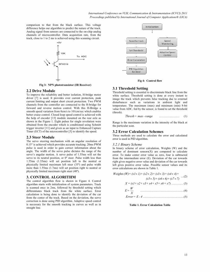
3. CONTROL ALGORITHM The control algorithm flow is shown in Figure 4. Control

algorithm starts with initialization of system parameters. Track

is scanned once in 2ms, followed by threshold setting which

differentiates black track from the white surface. Error

calculation is being done to identify the deviation of the car from the center of the track. Based on the deviation, the servo

correction is done using PID algorithm. Adaptive speed control

is necessary for the smooth tracking in curves as well as in

straight line.

Fig 4: Control flow

3.1 Threshold Setting Threshold setting is essential to discriminate black line from the

white surface. Threshold setting is done at every instant to

image the track which prevents false tracking due to external

disturbances such as variations in ambient light and

temperature. The maximum (max) and minimum (min) 8-bit

value from ADC, fed by the sensor, is found to set the threshold

(thresh).

range-max=Thresh ………………… (1)

Range is the maximum variation in the intensity of the black at

the particular scan.

3.2 Error Calculation Schemes Three methods are used to calculate the error and calculated

error is used in PID algorithm.

3.2.1 Binary Scheme In binary scheme of error calculation, Weights (W) and the

number of dominant sensors(X) are computed to calculate

error. To make center error value as zero, four is subtracted from the intermediate error (E). Deviation of the car towards

right gives negative error value and deviation of the car towards

left gives positive error value. Possible sensor values and its

error calculations are shown in Table 1.

7) (s7 + 6) (s6 + 5) (s5

+ 4) (s4 + 3) (s3 + 2) (s2 + 1) (s1 = (W) Weights

×××

××××....(2)

s7)+s6+s5+s4+s3+s2+(s1 =X ………… (3)

X

W = E ………………………………………(4)

4-E = Error ……………………………………(5)

Table 1. Error Calculation Table



14

3.2.2 Gray Scale Scheme 1. Compensation ratio (CR) is calculated.

)valuewhitevalueblack(CR

−=

256 ………………….. (6)

2. Compensated reading is found using CR

If reading > black value then reading=black

If reading < white value then reading=white

CR white)- (reading = reading dCompensate × …... (7)

3. Sort the values and take two maximum values and find the

position and error:

value) max (second read) value max of (index512 =Pos +×

………………. (8) NOTE: second max value should be subtracted if the second max value's index value is less than 3 else add.

pos -1568 = Error ……………………………………… (9)

NOTE: if pos is greater than 1568 error=pos-1568.

3.2.3 X-Y Scheme 1. Threshold is set similar to binary scheme and sensor values

are assigned as ‘1’ if reading > threshold; ‘0’ if reading < threshold.

2. Error is calculated using xerror and yerror.

xerror indicates the three sensor values (sensor 0 to 3) yerror

indicates the three sensor values (sensor 3 to 6)

xerror -yerror = Error …………………………… (10)

If equation (10) is positive, it justifies the car is towards left

from the center of the track, right steer value is given to bring

back the car to the center of the track and if equation (10) value

is negative, then the car is towards right from the center of the

track, left steer value is given to bring back the car to the centre

of the track.

3.3 Proposed Algorithm for Steering Error values from the error calculation schemes are fed to the

control algorithm, for accurate steering, as shown in Figure 5.

Fig 5: Steer control algorithm

Proportional (P) value is calculated using Kp (proportional constant) and error.

Error K=P p × …..……………………………… (11)

Fig 6: Steer vs Error using proportional controller

Figure 6 shows relationship between steer (PWM) and error.

There is a linear relationship only in the range -15 to +15. In order to attain linearity we go for integral and derivative

controller along with proportional.

When the car deviates from center to right, then error must be

accumulated (Acc). In case if the car moves from right to

center then the error must be subtracted from the accumulated value so as to bring back the car to center of the line. This is

accomplished by comparing present error with the previous

error(p_error) as shown in Figure 5. With integral constant (ki)

and derivative constant (Kd), integral and derivative action is

computed according to the equation 12 and 13. Correction

factor is calculated from the proportional and accumulated value as shown in equation 14. Final steer PWM value is

calculated using equation 15. Experimental result shows the

linearity in the steering throughout the range which is shown in

the Figure 7.

ikerrorAccAcc ×+= …………... (12)

dkerrorAccAcc ×−= …………… (13)

)AccP(corr += …………............. (14)

corr+er_valuecenter_ste= Steer ……………… (15)

S

1

S

2

S

3

S

4

S

5

S

6

S

7

X (No.

of 1’s)

Weights

(W)

E

=

W/X

Error

=

E-4

1 0 0 0 0 0 0 1 1 1 -3

1 1 0 0 0 0 0 2 3 1.5 -2.5

0 1 0 0 0 0 0 1 2 2 -2

0 1 1 0 0 0 0 2 5 2.5 -1.5

0 0 1 0 0 0 0 1 3 3 -1

0 0 1 1 0 0 0 2 7 3.5 -0.5

0 0 0 1 0 0 0 1 5 4 0

0 0 0 1 1 0 0 2 9 4.5 0.5

0 0 0 0 1 0 0 1 5 5 1

0 0 0 0 1 1 0 2 11 5.5 1.5

0 0 0 0 0 1 0 1 6 6 2

0 0 0 0 0 1 1 2 13 6.5 2.5

0 0 0 0 0 0 1 1 7 7 3



15

Fig 7: Steer vs Error using PID

3.4 Proposed Algorithm for Speed Control To make the car to track the entire lap at desired speed

irrespective of the curvature and terrain of the track, adaptive

speed control algorithm is proposed. Constant rotation value (CR) of the wheel is fixed for the constant speed of the car.

Current speed of the car (ROT) is measured and compared

periodically with CR. Based on the comparison result if the

current speed is greater that the desired speed (i.e.) ROT>CR

then the vehicle is slowed down by reducing the PWM to the constant duty value (i.e) 65 to make the vehicle to move in the

desired speed. If the speed of the vehicle decreases from the

desired speed (i.e.) ROT<CR then we increment ‘Ks’ for every

iteration which increases the speed by increasing the PWM

duty gradually according to equation 16 until the vehicle

reaches the desired speed. Equation 16 shows how the PWM value for the DC drive is assigned dynamically and they are

tabulated in Table 2. In table 2 the first row values are the speed

factor(Ks) value which is incremented for every iteration. The

first column value is the difference of Constant Rotation value

(CR) with the Current Speed (ROT). When this difference is

zero, vehicle moves in a desired speed hence the row values are 65 which is the PWM duty value for DC motor. When the

difference is more, the PWM duty value is increased for each

iteration to attain the desired speed. Different possible PWM

duty values with respect to the speed factor and speed

difference is shown in table 2. Thus the speed of the car is

dynamically varied to maintain the desired speed independent

of the road conditions. This is the adaptive speed control

method which is proposed. The entire flow is shown in the

Figure 8.

Fig 8: Adaptive speed control

ROT))-(CR(K+Const_duty=PWM_duty s × ……. (16)

Figure 9 shows the relationship between the three parameters

CR-ROT, Ks & PWM. From the Figure 9 it is clear that when

the speed of the car decreases due to more friction between

wheel and road, then the car will not move in the desired speed

even though the desired PWM duty value is given. The

difference (CR-ROT) is more for a long time then Ks parameter

will increase gradually for every iteration and increases the

PWM duty value to its maximum.

Table 2. Adaptive Speed PWM table

(CR-

ROT)\

KS

1 2 3 4 5 6 7 8

0 65 65 65 65 65 65 65 65

1 66 67 68 69 70 71 72 73

2 67 69 71 73 75 77 79 81

3 68 71 74 77 80 83 86 89

4 69 73 7 81 85 89 93 97

5 70 75 80 85 90 95 100 105

6 71 77 83 89 95 101 017 113

7 72 79 86 93 100 107 114 121

Fig 9: Adaptive speed 3D

Fig 10: Steer and Speed Control Structure

3.5 Combined Steer and Speed Control



16

Figure 10 shows the complete system structure which is

implemented for both steering control and speed control of

smart car. The adaptive speed control algorithm takes the input from the encoder and calculates the desired PWM for the DC

motor drive for longitudinal control. IR Sensor module located in front of the car identifies the position of the car in the track

through the proposed error calculation techniques and applying

PID control for error correction and the correction is achieved

by servomotor which is connected to the front wheel of the car

as shown in figure 10. Thus with the proposed speed control

and steer control algorithms it is possible to complete the lap within very short duration with constant speed.

4. TRACK SPECIFICATION Proposed track has 28m length and 2.5cm width with varying

turn radius not less than 60cm as shown in Figure 11. The smart

car under test is kept in the starting point in the track ( Black

intersecting point) and the car is allowed to travel in ten

different radius of curves and finally it comes to the starting

point. The time taken for the car to complete the lap is taken as

the refernce. The car is tested with different algorithms and the

parameters like the speed accuracy and tracking accuracy is

monitored and the proposed alogrithm makes the car to travel

smoothly in all the ten different curves and completes the lap in

shorter time.

Fig 11: Proposed track

5. EXPERIMENTAL RESULTS To optimse Kp, Ki and Kd values for the three proposed schemes

several iterations was carried out to achieve the better speed

accuracy and tracking accuracy. Code Warrior IDE[6] is used

for the sofware development.

5.1 Speed Accuracy Adjustment of speed towards the desired speed gives the speed

accuracy. Encoder samples are obtained in every 12.5ms and the

speed of the car is measured and the speed accuracy is calculated

using the expression (17) and (18) and the results are plotted in table 3. Table 3 shows the lap completion time and speed

accuracy of different algorithms. X-Y algorithm takes more time

to complete the lap and the speed accuracy is just 69.04%.

Binary algorithm completes the lap in 28.1 seconds and the

speed accuracy is 98.62%. From the test results binary scheme

gives better speed accuracy. This justifies the proposed speed

control method gives better performance over the entire track.

Ten curves of different radius does not affect the speed of the car

and proposed speed control algorithm gives smooth

performance in all the curves.

SpeedDesired

cetanDisLap)RT(eferenceTimRe = ……………… (17)

100100 ×

−−=

RT

)RTTimeMeasured(%inccuracyASpeed

………..(18)

Table 3. Adaptive Speed

Algorithm Lap Completion

time (sec.)

Speed Accuracy

( %)

Binary 28.1 98.62

Gray Scale 32.7 82.03

X-Y 36.3 69.04

5.2 Tracking Accuracy Deviation from the normal course of the track has poor tracking

accuracy and zero deviation from the track has 100% tracking

accuracy. The constant speed is fixed for three algorithms and to

find the tracking accuracy of the car, the total 28m track is

scanned at the rate of 500Hz to get 14,000 samples out of which,

the car stays, 63.6% around center, 17.17% to the left and

17.58% to the right which shows better tracking accuracy of the

binary scheme where the gray scale and X-Y scheme makes the

car to stay in the center less than 50%. This analysis proves that

the tracking accuracy is better for binary scheme than the other two schemes.

Guard mechanism starts functioning when the car steers out of

track by identifying the all white condition. It helps the car to

return back to the track by analyzing the track record.

Experimental results revealed range value as 20. The threshold

recognizes all the sensor values as white in the following two

conditions.

Case 1: 7th sensor senses very low black track value.

Sensor 0 1 2 3 4 5 6

Reading 8 8 8 9 9 9 25

Case 2: All sensors sense black track value.

Sensor 0 1 2 3 4 5 6

Reading 244 246 240 241 242 241 241

In-order to overcome the above conditions, the difference between two maximum values is used and the range should be

less than 20. Experimental results proved better performance,

even with different lighting setup and track complexity.

6. CONCLUSIONS AND FUTURE SCOPE The three algorithms were compared on the basis of various

parameters like speed, tracking time and tracking efficiency. The

Gray scale scheme proved to be efficient in terms of sensitivity

but it lost out to binary scheme in terms of speed accuracy. So a

trade off would be required between these two depending upon

the application where speed matters over tracking accuracy or

vice versa. With reference to our base paper, our proposed

method proved efficient in terms of tracking and speed accuracy. This method is suitable even when the track has inclined or

declined slopes.

It is believed that autonomous navigating cars will be the next big thing of the future. There will be a need where the car

would be required to park in the allotted space autonomously



17

by sensing the parking lane. Also in most of the countries

where lane driving is prevalent, the speed has to be adaptively

changed on detection of a lane change. So this smart car with

its robust line following and detection capability will come in

handy. It is planned to incorporate wireless protocol for

communication between the cars which will serve greatly to

avoid collision and also to share the relative information about

one another thereby helping in traffic management.

7. ACKNOWLEDGMENTS

The authors acknowledge Management and Principal, PSG College of Technology for providing the enough lab facilities

for implementing and testing the algorithms. Authors like to

thank Freescale Semiconductors, for their support in hardware

and software design and development.

8. REFERENCES [1] Mehran Pakdaman, M. Mehdi Sanaatiyan, “Design and

implementation of Line following robot”, Second

International Conference on Computer and Electrical Engineering, 2009.

[2] M.Zafri Baharuddin, “Analyst of Line Sensor

Configuration for Advanced Line Follower Robot”,

University Tenaga National.

[3] Cao Quoc Huy, “ Line Follower Robot”, University UPG din Ploiesti.

[4] P.Heyrati, A.Aghagani, “Science of Robot Design and Build Robot”, Azarakhsh Publication, 2008.

[5] Freescale MC9S12XDP512RMV2 Datasheet, Rev. 2.21, October 2009.

[6] Freescale CodeWarrior IDE, Version 5.0.

[7] Freescale MC339331 datasheet, Throttle Control H-Bridge, Rev 2.0, 2008.

[8] OSRAM Opto Semiconductor, SFH4550 datasheet, High power IR Emitter.

[9] OSRAM Opto Semiconductor, SFH 314 datasheet, NPN phototransistor.

[10] Siemens, SMBT3904 datasheet, NPN Silicon Switching Transistor.

[11] Schmitt trigger Inverters, HD74LS14 datasheet.

[12] Precision Dual Operational Amplifier, TLC272 datasheet.

[13] Slotted couplers, MOC7811 datasheet.

Design of Automatic Steering Control and Adaptive Cruise ... · PDF fileInternational...

Documents

Transcript of Design of Automatic Steering Control and Adaptive Cruise ... · PDF fileInternational...