Clemson UniversityTigerPrints

All Dissertations Dissertations

5-2016

Design of a Wide Area Controller UsingEigenstructure Assignment in Power SystemsParimal SarafClemson University, psaraf@g.clemson.edu

Follow this and additional works at: https://tigerprints.clemson.edu/all_dissertations

Part of the Computer Engineering Commons, and the Electrical and Computer EngineeringCommons

This Dissertation is brought to you for free and open access by the Dissertations at TigerPrints. It has been accepted for inclusion in All Dissertations byan authorized administrator of TigerPrints. For more information, please contact kokeefe@clemson.edu.

Recommended CitationSaraf, Parimal, "Design of a Wide Area Controller Using Eigenstructure Assignment in Power Systems" (2016). All Dissertations. 2304.https://tigerprints.clemson.edu/all_dissertations/2304

DESIGN OF A WIDE AREA CONTROLLER USING EIGENSTRUCTURE ASSIGNMENT IN POWER SYSTEMS

______________________________________________________________

A DissertationPresented to

the Graduate School ofClemson University

______________________________________________________________

In Partial Fulfillmentof the Requirements for the Degree

Doctor of PhilosophyElectrical and Computer Engineering

______________________________________________________________

byParimal Saraf

May 2016

______________________________________________________________

Accepted by:Dr. Elham B. Makram, Committee Chair

Dr. Richard GroffDr. Taufiqar Khan

Dr. Anthony MartinDr. Ramtin Hadidi

ABSTRACT

Small signal stability has become a major concern for power system operators around

the world. This has resulted from constantly evolving changes in the power sys-

tem ranging from increased number of interconnections to ever increasing demand of

power. In highly stressed operating conditions, even a small disturbance such as a

load change can make the system unstable resulting in small signal instability. The

main reason for small signal instability in power systems is an inter-area mode/s be-

coming unstable. Inter-area modes involve a group of generators oscillating against

each other. Traditionally, power system stabilizers installed on the synchrous ma-

chines were used to damp the inter-area modes. However, they may not be very

suitable to perform the job since they use local I/O signals which do not have a

good controllability/observability of the inter-area modes. Recent advancements in

phasor measurement technology has resulted in fast acquisition of time-synchronized

measurements throughout the system. Thus, instead of using local controllers, an

idea of a wide area controller (WAC) was proposed by the power systems community

that would use global signals. This dissertation demonstrates the design of a WAC

using eigenstructure assignment technique. This technique provides the freedom to

assign a few eigenvalues and corresponding left or right eigenvectors for Multi-Input-

Multi-Output (MIMO) systems. This technique forms a good match for designing a

WAC since a WAC usually uses multiple I/O signals and a power system only has

a few inter-area modes that might lead to instability. The last chapter of this dis-

sertation addresses an important aspect of controller design, i.e., robustness of the

controller to uncertainties in operating point and time delay of feedback signals. The

operating point of a power system is highly variable in nature and thus the designed

ii

WAC should be able to damp the inter-area modes under these variations. Also, a

transmission delay is associated due to routing of remote signals. This time delay is

known to deteriorate the performance of the controller. A single controller will be

shown to achieve robustness against both these uncertainties.

iii

Dedication

This dissertation is dedicated to my grand parents, parents and sister.

iv

Acknowledgements

I wish to express my gratitude to my adviser, Dr. Elham Makram for her technical

guidance, support, kindness and patience throughout the period of research and study

at Clemson University.

I want to thank Dr. Ramtin Hadidi for providing valuable technical inputs and always

being supportive as a teacher and a friend.

I want to thank Dr. Richard Gro, Dr. Tauqar Khan and Dr. Anthony Martin for

agreeing to be on my committee.

I thank all the fellow students in my group, especially Karthikeyan Balasubrama-

niam and Puspal Hazra, with whom I had a lot of fruitful discussions throughout the

course of my period at the university. Many thanks go to my friends Prateek Kaul,

Natraj Chandrasekharan, Rohan Galgalikar, Saurabh Prabhu, Sara Touchet for their

constant support and encouragement.

I thank the Department of Electrical and Computer Engineering and the professors

with whom I worked through the course of my degree. They helped develop and

improve my knowledge of electrical engineering.

Last but not the least I want to thank my parents, grandparents and sister who

have always been encouraging and patient. A very special thanks to my lovely wife,

Sumedha. Her love and support has made this journey less strenuous.

v

Contents

1. Introduction 1

1.1. Damping of Inter-area oscillations . . . . . . . . . . . . . . . . . . . . 2

1.2. Wide Area Measurement and Control . . . . . . . . . . . . . . . . . . 5

1.3. Eigenstructure Assignment . . . . . . . . . . . . . . . . . . . . . . . . 6

1.4. Dissertation Contents . . . . . . . . . . . . . . . . . . . . . . . . . . . 9

2. Power System Modeling and Small Signal Stability 11

2.1. Dynamic Modeling . . . . . . . . . . . . . . . . . . . . . . . . . . . . 11

Synchronous Machine . . . . . . . . . . . . . . . . . . . . . . . . . . . 11

Excitation Systems . . . . . . . . . . . . . . . . . . . . . . . . . . . . 14

Governor . . . . . . . . . . . . . . . . . . . . . . . . . . . . . . . . . . 15

Power System Stabilizer (PSS) . . . . . . . . . . . . . . . . . . . . . . 16

Static VAR Compensator (SVC) . . . . . . . . . . . . . . . . . . . . . 17

2.2. Small Signal Stability and Linearized Model of a Power System . . . 17

3. Design of a Wide Area Controller 23

3.1. Controller Design Using Quadratic Programming . . . . . . . . . . . 25

Partial Right Eigenstructure Assignment . . . . . . . . . . . . . . . . 25

Dynamic Compensator . . . . . . . . . . . . . . . . . . . . . . . . . . 29

Quadratic Programming . . . . . . . . . . . . . . . . . . . . . . . . . 31

3.2. I/O Signal Selection and Time Delay of Feedback Signals . . . . . . . 33

3.3. Multi-model Optimization for Controller Design . . . . . . . . . . . . 37

3.4. Results and Discussion . . . . . . . . . . . . . . . . . . . . . . . . . . 40

Controller Design for the Nominal Model . . . . . . . . . . . . . . . . 40

vi

Multi-model optimization for controller design . . . . . . . . . . . . . 45

3.5. Discussion . . . . . . . . . . . . . . . . . . . . . . . . . . . . . . . . . 53

4. Robustication of a Wide Area Controller 54

4.1. Obtaining the Extended Dynamic System . . . . . . . . . . . . . . . 56

4.2. Setting the Optimization Problem . . . . . . . . . . . . . . . . . . . . 57

Method 1 . . . . . . . . . . . . . . . . . . . . . . . . . . . . . . . . . 58

Method 2 . . . . . . . . . . . . . . . . . . . . . . . . . . . . . . . . . 63

4.3. Approach I . . . . . . . . . . . . . . . . . . . . . . . . . . . . . . . . 68

4.4. Approach II . . . . . . . . . . . . . . . . . . . . . . . . . . . . . . . . 74

Linear Fractional Transform . . . . . . . . . . . . . . . . . . . . . . . 75

Destabilizing Perturbation . . . . . . . . . . . . . . . . . . . . . . . . 78

Results . . . . . . . . . . . . . . . . . . . . . . . . . . . . . . . . . . . 79

4.5. Discussion . . . . . . . . . . . . . . . . . . . . . . . . . . . . . . . . . 80

5. Conclusions and Future Work 86

5.1. Conclusions . . . . . . . . . . . . . . . . . . . . . . . . . . . . . . . . 86

5.2. Future Work . . . . . . . . . . . . . . . . . . . . . . . . . . . . . . . . 87

A. IEEE 68 bus base-case system data 100

B. Implementing controller design in PST 107

vii

List of Figures

2.1. Schematic of a synchronous machine with two poles . . . . . . . . . . 12

2.2. Block diagram of a simple excitation system . . . . . . . . . . . . . . 14

2.3. Block diagram of a simple governor-turbine system . . . . . . . . . . 16

2.4. Block diagram of a PSS . . . . . . . . . . . . . . . . . . . . . . . . . 16

2.5. Block diagram of a SVC . . . . . . . . . . . . . . . . . . . . . . . . . 17

2.6. Schematic of a WAC . . . . . . . . . . . . . . . . . . . . . . . . . . . 22

3.1. A owchart explaining the controller design algorithm . . . . . . . . . 34

3.2. time delay in one of the output signals . . . . . . . . . . . . . . . . . 36

3.3. IEEE 68 bus system with the WAC . . . . . . . . . . . . . . . . . . 41

3.4. IEEE 68 bus system with the WAC . . . . . . . . . . . . . . . . . . 44

3.5. Comparison of performance of Knom1(s) and Knom2(s) . . . . . . . . . 47

3.6. Susceptance of the SVCs during fault for all three operating conditions

when using Knom2(s) . . . . . . . . . . . . . . . . . . . . . . . . . . . 48

3.7. Comparison of the performance of Knom2(s) and Krobust(s) connected

to the nominal and delayed system . . . . . . . . . . . . . . . . . . . 49

3.8. Comparison of the performance of Knom2(s) and Krobust(s) for OP1

and dierent values of time delays . . . . . . . . . . . . . . . . . . . . 50

3.9. Comparison of the performance of Knom2(s) and Krobust(s) for OP2

and dierent values of time delays . . . . . . . . . . . . . . . . . . . . 51

3.10. Comparison of the performance of Knom2(s) and Krobust(s) for OP3

and dierent values of time delays . . . . . . . . . . . . . . . . . . . . 52

4.1. Algorithm showing the steps to be followed in Method 1 . . . . . . . 64

viii

4.2. A line to connected by two points to one point each to the left and

right of the line . . . . . . . . . . . . . . . . . . . . . . . . . . . . . . 65

4.3. A line to connected by two points to one point each to the left and

right of the line . . . . . . . . . . . . . . . . . . . . . . . . . . . . . . 66

4.4. Algorithm showing the steps to be followed in Method 2 . . . . . . . 68

4.5. Closed-loop eigenvalues with K(s), Kmethod1(s) and Kmethod2(s) con-

nected in feedback to system model OP1 . . . . . . . . . . . . . . . . 71

4.6. Closed-loop eigenvalues with K(s), Kmethod1(s) and Kmethod2(s) con-

nected in feedback to system model OP2 . . . . . . . . . . . . . . . . 71

4.7. Closed-loop eigenvalues with K(s), Kmethod1(s) and Kmethod2(s) con-

nected in feedback to system model OP3 . . . . . . . . . . . . . . . . 72

4.8. Angle dierence between machines 15 and 16 for a ten-cycle, three-

phase fault at bus 52, OP1 . . . . . . . . . . . . . . . . . . . . . . . . 72

4.9. Angle dierence between machines 15 and 16 for a ten-cycle, three-

phase fault at bus 52, OP2 . . . . . . . . . . . . . . . . . . . . . . . . 73

4.10. Angle dierence between machines 15 and 16 for a ten-cycle, three-

phase fault at bus 52, OP3 . . . . . . . . . . . . . . . . . . . . . . . . 73

4.11. LFT representation of the system . . . . . . . . . . . . . . . . . . . . 77

4.12. Eigenvalues of the base-case and worst-case models . . . . . . . . . . 79

4.13. Closed-loop eigenvalues with K(s), Krobust1(s) and Krobust2(s) con-

nected in feedback to system model OP1 . . . . . . . . . . . . . . . . 81

4.14. Closed-loop eigenvalues with K(s), Krobust1(s) and Krobust2(s) con-

nected in feedback to system model OP2 . . . . . . . . . . . . . . . . 81

4.15. Closed-loop eigenvalues with K(s), Krobust1(s) and Krobust2(s) con-

nected in feedback to system model OP3 . . . . . . . . . . . . . . . . 82

ix

4.16. Angle dierence between machines 15 and 16 for dierent values of

Pload,42 using K(s) . . . . . . . . . . . . . . . . . . . . . . . . . . . . 82

4.17. Angle dierence between machines 15 and 16 for dierent values of

Pload,42 using Krobust1(s) (solid) and Krobust2(s) (dashed) . . . . . . . . 83

4.18. Angle dierence between machines 15 and 16 for dierent values of

time delay using K(s) . . . . . . . . . . . . . . . . . . . . . . . . . . 83

4.19. Angle dierence between machines 15 and 16 for dierent values of

time-delays using Krobust1(s) (solid) and Krobust2(s) (dashed) . . . . . 84

A.1. Bus data . . . . . . . . . . . . . . . . . . . . . . . . . . . . . . . . . . 101

A.2. Bus data continued . . . . . . . . . . . . . . . . . . . . . . . . . . . . 102

A.3. Line data . . . . . . . . . . . . . . . . . . . . . . . . . . . . . . . . . 103

A.4. Line data continued . . . . . . . . . . . . . . . . . . . . . . . . . . . . 104

A.5. Line data continued . . . . . . . . . . . . . . . . . . . . . . . . . . . . 105

A.6. Exciter data . . . . . . . . . . . . . . . . . . . . . . . . . . . . . . . . 105

A.7. PSS data . . . . . . . . . . . . . . . . . . . . . . . . . . . . . . . . . . 106

A.8. turbine-governor data . . . . . . . . . . . . . . . . . . . . . . . . . . . 106

A.9. Static Var compensator data . . . . . . . . . . . . . . . . . . . . . . . 106

B.1. Flowchart representing the steps to be followed to obtain the controller 108

B.2. Steps to be followed to determine the worst-case model . . . . . . . 109

B.3. Adding the controller to PST . . . . . . . . . . . . . . . . . . . . . . 110

x

List of Tables

3.1. Residues of top 10 controllable eigenvalues . . . . . . . . . . . . . . . 42

3.2. Assigned eigenvalues and their damping ratios . . . . . . . . . . . . . 42

3.3. Operating points for validating the robustness of the controller . . . . 44

4.1. Dierent operating points for ensuring robustness . . . . . . . . . . . 69

xi

1.Introduction

Deregulation and evolution of power markets has led to increased interconnections in

the power system leading to complex power ows. The aim of these interconnections

is primarily to increase the reliability of operation of the system and allow trading of

power between the interconnected areas. Certain operating conditions involve large

amounts of power are transferred over these interconnections which results in the

system being operated very close to instability. Moreover, the load in the system is

continuously increasing without installation of new infrastructure. Thus it is very

important to utilize the existing resources eciently to ensure reliable and stable

operation of the grid.

An interconnected power system is composed of multiple dynamic components

such a rotating machines, exible A.C transmission systems (FACTS) devices, dy-

namic loads etc. Similar to any dynamic system, the response of a power system to

disturbances is governed by the modes present in the system. These modes can be

categorized into the following four types:

a) Local modes: These modes involve a machine swinging against the rest of the

system. The oscillations associated with these modes are localized to one machine or

a small portion of the system.

b) Inter-area modes: These modes involve a group of machines oscillating against

another group of machines connected through a weak transmission system. These

modes are more complex to study and control as they involve multiple machines

participating in these modes.

c) Control modes: These modes are associated with poorly tuned controllers in the

system such as exciters, governors etc.

1

d) Torsional modes: These modes are associated with turbine-generator shaft sys-

tem rotational components.

When a disturbance happens in a system, these modes are excited. These dis-

turbances can be either small changes in the system such as a load change or large

changes such a fault. In order for a system to be small-signal stable, all these modes

have to be well-damped. If any of the modes is poorly damped, appropriate con-

trol action has to be taken. The challenges involved in damping inter-area modes as

opposed to the other modes are that multiple synchronous machines participate in

them and under stressed conditions even a small disturbance can make them unsta-

ble. Some major systems across the world known to have low frequency inter-area

oscillations are: Hydro-Quebec (0.6 Hz) [1], Western Interconnected System (0.4 - 1

Hz) [2], Brazilian system (0.15-0.25 Hz) [3], UCTE interconnection in Europe (0.19

- 0.36 Hz) [4]. An important aspect associated with inter-area modes is that they

are sensitive to operating conditions. As a result, they have been a major reason

for blackouts across the world. The 1996 WECC blackout was a result of a 0.22

Hz inter-area mode becoming unstable due a fault in an already stressed system [5].

The recent 2003 Eastern Interconnect blackout also had an unstable 0.6 Hz inter-area

mode after a set of contingencies in the system [6]. Due to the implications of these

low frequency modes on the stability of the system, they also limit the amount of

power that can be transmitted from one region to another.

1.1. Damping of Inter-area oscillations

Traditionally, Power system stabilizers (PSS), installed on top of the excitation system

of the synchronous generators were used for damping electromechanical oscillations in

a power system. PSSs were tuned to ensure the damping of local modes. The damp-

2

ing of these modes is achieved by providing damping torque in phase with speed of

the synchronous machines at the natural frequency of the mode through utilization of

their excitation systems. The feedback signals used for PSSs were local speed, accel-

eration or power output signals [7]. In a lot of systems, the I/O signals to the PSS do

not have a good controllability/observability of the inter-area modes. Therefore, mul-

tiple PSSs need to be coordinated to enhance the damping of these modes. In [8], the

impact of parameters and locations of a PSS on the local as well as inter-area modes

has been presented. It is invariably the case that a few chosen PSSs are required to

participate in the damping of poorly damped inter-area modes. In [9], residue anal-

ysis of the stabilizing control loop has been used to select the most eective PSSs in

the system and then a Newton Raphson algorithm has been implemented to achieve

partial pole assignment for assigning poorly damped modes at better locations. One

issue with using PSSs for damping these low frequency oscillations is that they tradi-

tionally use local signals that may not have good observability of these modes. Also,

it is predicted that with the advent of new technologies, the local modes in the system

are expected to be in the range of 4 Hz [10]. Thus, utilizing a PSS for damping local

as well as inter-area modes would require them to operate in a wider bandwidth.

The advent of high speed FACTS devices has enabled better control of these oscil-

lations as they are installed close to the tie lines. Series FACTS devices are used to

regulate the power ows on tie lines whereas shunt devices regulate bus voltages by

injecting reactive power at a bus. A previous work has compared the performance

of Static VAr Compensator (SVC), Static Synchronous Compensator (STATCOM)

and PSS for damping power system oscillations [11]. In [12, 13], the integration of

the dynamic models of FACTS into the power system and the tuning of the parame-

ters of FACTS devices to achieve damping of oscillations has been shown. In [14], a

non-linear control technique applied on a Unied Power Flow Controller (UPFC) has

3

been used to damp the inter-area oscillations. In [15], a unied model of a system

comprising of three dierent types of FACTS devices is developed and their eective-

ness in suppressing oscillations is studied using the damping torque analysis. In [16],

a supplementary power oscillation damping (POD) loop, comprising of set of lead-

lag blocks, on a Thyristor Controlled Switched Capacitor (TCSC) has been tuned to

damp the inter-area oscillations in a power system.

Similar to PSSs, POD control loop on FACTS devices can be coordinated with other

local controllers in the system. In [17], a nonlinear optimization based framework for

simultaneous coordination of supplementary power oscillation damping (POD) con-

trol loop on FACTS devices and PSSs has been detailed. The objective function

consists of minimizing a cumulative damping index with the constraint that the op-

timizing variables are within minimum and maximum limits. Another work uses a

Quasi-Newton algorithm to minimize a quadratic performance index over a period

of time [18]. The method again involves coordination of PSSs and POD loops on

FACTS devices to minimize the deviations in tie-line powers as well as generator

power outputs. The objective function used is a non-explicit function and thus the

algorithm is integrated to a simulation platform to optimize the parameters of the

controllable devices. Reference [19] presents an iterative optimization technique that

coordinates PSSs and FACTS devices in the system to iteratively relocate the poorly

damped eigenvalues to better locations.

Based on the references presented, it is clear that local controllers are not very

eective in damping inter-area oscillations. They have a positive impact on damp-

ing only when coordinated with other local controllers in the system which might

not be the best available option. Further, reference [20] presents a concept of nearly

decentralized xed modes (NDFM) that are inter-area modes that cannot be appre-

ciably shifted using any sort of local controllers in the system. This is because as

4

mentioned earlier inter-area modes are not very controllable/observable using local

signals. In [21], it has been shown that a detrimental interaction is possible between

various local controllers such as PSSs, FACTS POD due to lack of knowledge of the

global state variables.

1.2. Wide Area Measurement and Control

In order to address the issues faced by local controllers in damping inter-area oscilla-

tions, a WAC that utilizes global signals and operates on top of the local controllers

has been proposed in [22]. The advantage of using this approach is that it gives

the freedom to select the I/O signals of the controller such that inter-area modes

have a good controllability/observability metric. In [22], it has been mentioned that

under certain scenarios an inter-area mode might be controllable from one area and

observable from another. In [23], it has been shown that remote signals rather than

local signals give better controllability of the inter-area modes. A majority of previ-

ous works use methods based on residuals or/and geometric measures to select I/O

signals for the WAC [2426]. Other available techniques for selecting I/O signals are

based on Hankel singular values (HSV) and relative gain array (RGA) [27].

New measurement technology utilizing Phasor Measurement Units (PMU) has

made it possible to get fast measurements of various system variables such as volt-

ages, currents, frequencies etc. at sampling rates ranging between 30 samples/sec

to 120 samples/sec [28]. The unique feature of this technology is that the measure-

ments throughout the network are time synchronized which enables obtaining a wider

picture of the system. Due to a constraint on the number of PMUs that can be in-

stalled in the system, they are only deployed at certain strategic locations. These

time synchronized measurements from dierent parts of the system can be fed as

5

remote signals for designing WACs. In [29], a PSS utilizing local as well as a re-

mote signal obtained from a PMU is tuned to damp inter-area oscillations. In [30],

a decentralized/hierarchical MIMO WAC to damp oscillations is designed using an

optimization framework utilizing a modal performance measure over a period of time.

In [31], a multi-agent based framework is used where a supervisory PSS having an H-

innity control loop is coordinated with local PSSs in each area to damp oscillations

in an eective way. A fuzzy logic based rule is used to switch the supervisory PSS

robust control loop. In [32], an optimal controller design with structural constraints

is proposed with a two-level control structure. However, model order reduction is

required to achieve faster convergence of the algorithm presented. Also, one of the

important factors considered in this paper is signal transmission delay when using

remote signals. In [33], a mixed-objective, output feedback H2/H-innity synthesis

with regional pole placement is presented for designing a WAC for damping inter-area

oscillations. The work adopts a hierarchical control structure where the WAC oper-

ates on top of the local controllers such as PSSs. A model order reduction technique

is employed when using frequency domain robust control techniques in order to save

time on computation.

1.3. Eigenstructure Assignment

A WAC designed for a realistic sized power system typically involves selecting multi-

ple I/O signals to make the inter-area modes controllable/observable. Reference [30]

has presented a very detailed description of a procedure for designing a MIMO WAC

for a large power system. The paper starts with a detailed discussion on selecting the

feedback signals and the local controllers that participate in the global control scheme.

The parameters of the centralized controller are obtained as a solution to a nonlin-

6

ear optimization problem that minimizes a modal performance index over time. The

paper also presents a comparison of using a decentralized or a global hierarchical con-

trol scheme. Even though the work is based on using a modal performance measure,

it does not exploit the design freedom available for MIMO systems to modify spe-

cic eigenvectors along with the corresponding eigenvalues for improving the dynamic

performance of the system. In [34], it was identied that state feedback for MIMO

systems provides additional design freedom on top of assigning closed-loop eigenval-

ues. This controller design method that exploits the degrees of freedom provided

by both eigenvalues and eigenvectors for MIMO systems is known as eigenstructure

assignment and has been extensively used in aerospace applications [35]. According

to [36], all the closed-loop eigenvalues of a MIMO dynamic system can be assigned

using output feedback if the sum of the number of inputs and outputs is more than

the number of state variables in the system. However, in a realistic power system,

this condition will never be satised. Furthermore, it would be a worthless activity

to assign all the eigenvalues in a power system since only a few of them dominate the

dynamic behavior.

There are only a few existent applications of eigenstructure assignment technique

for designing controllers in power systems. In [37], a framework for implementing a

decentralized control scheme (proportional output feedback based PSSs on machines)

based on eigenstructure assignment has been successfully used to damp inter-area os-

cillations as well as reduce the participation of these modes in certain machine speeds.

However, power systems throughout the world have lead-lag type PSSs installed on

them. Therefore, replacing them with proportional feedback type PSSs is not a vi-

able option. In [38], a partial left eigenstructure assignment has been presented to

design a controller for a doubly fed induction generator (DFIG) in order to reduce

the excitation of an inter-area mode and a shaft mode. A dynamic compensator

7

has been employed to increase the degrees of freedom available for eigenstructure

assignment. A multi-objective optimization problem with parametric vectors associ-

ated with selected left eigenvectors as the optimizing variables is formulated. In [39],

partial right eigenstructure assignment technique has been used to design a robust

power system stabilizer. Similar to [38], parametric vectors associated with certain

right eigenvectors are used as optimizing variables. The optimization algorithm in-

corporates multiple operating points in order to attain robustness against operating

point changes. Both of these references deal with the design of a local controller on

a machine.

The main focus of this dissertation is to study the application of eigenstructure

assignment for designing a hierarchical WAC for enhancing the damping of poorly

located inter-area modes. The core objectives of this thesis can be sub-divided into

two parts:

1) The controller should be capable of assigning the poorly damped inter-area

modes to user-specied locations while also assigning the corresponding closed-loop

right eigenvectors. The number of I/O signals utilized for achieving the assignment

should be less but at the same time should have sucient controllability/observability

of the poorly damped inter-area modes. Since a WAC uses remote I/O signals, the

issue of time delay of feedback signals should be addressed in the controller design

algorithm. The controller should not only perform for a xed time delay but should

also be robust to uncertainty in time-delay of feedback signals.

2) The operating conditions of a power system constantly vary throughout the day.

Therefore, it is very important that the controller should be robust to changes in

operating conditions. In other words, the controller should be capable of improving

the damping of inter-area modes of interest under varying operating conditions. This

performance requirement should be satised in addition to the controller being robust

8

to uncertainty in time-delay of feedback signals.

1.4. Dissertation Contents

Chapter 2 provides a basic background of modeling various dynamic components in

a power system and describes the small-signal analysis of a linearized power sys-

tem model around an operating point. Chapter 3 presents a detailed description of

eigenstructure assignment technique applied to the design of a WAC. A quadratic pro-

gramming based approach has been used to obtain the dynamic compensator based

controller. Two projection techniques have been presented and compared for assign-

ing the closed-loop right eigenvectors corresponding to the poorly damped inter-area

modes. A multi-model optimization scheme has been presented in the later part of

the chapter that makes the designed controller robust to uncertainty in time delays of

feedback signals. The algorithm has been applied on the IEEE 68 bus system and the

performance of the controller in improving the damping of poorly located inter-area

modes has been validated.

Chapter 4 addresses the issue of robustness of the controller to changing operating

conditions. A multi-model optimization approach, dierent from the one presented

in chapter 3, has been used to tune a WAC obtained from chapter 3 in order to

make it robust. Two dierent approaches have been presented to select the models

to be included in the multi-model optimization. The rst approach uses models that

are known to be stressed operating conditions of the system. The second approach

presents a method to select models such that the designed controller is robust to

changes in a specic parameter of the system. The second approach also accounts

for variability in time delay of feedback signals. Two dierent methods based on

eigenstructure assignment and rst order eigenvalue sensitivity have been used to

9

formulate the optimization problem. At the end of chapter 4, a controller that is

robust to operating point changes as well as uncertainty in time-delay of feedback

signals is obtained. Similar to chapter 3, this controller has been designed, tested and

validated for the IEEE 68 bus system.

Chapter 5 provides the conclusions of this dissertation and presents the avenues for

future research in this area. There is an appendix that aids in understanding some

of the material presented in this dissertation.

10

2.Power System Modeling and

Small Signal Stability

The main focus of this chapter is to provide a background on modeling and stability

of interconnected power systems. Since the essence of this dissertation is the analysis

and control of inter-area oscillations, more focus is placed on small-signal stability of

the system.

An interconnected power system comprises of a number of dynamic devices that

need to be modeled and combined together to obtain a unied non-linear dynamic

model of the system. This non-linear model is linearized around an operating point

to obtain the state space model of the system and an eigen-analysis is performed on

this model to determine the eigenvalues and eigenvectors of the dynamic system. The

relationship of eigenvalues and eigenvectors with the dynamic response of the system

will form the foundation for the future chapters.

2.1. Dynamic Modeling

Synchronous Machine

Synchronous machines form the primary source of electric energy in the system. They

form the basis of power system stability since they govern the dynamics of the system.

Power system stability is the ability of keeping the interconnected synchronous ma-

chines in synchronism. Therefore, the understanding of their modeling and dynamic

behavior is of utmost importance. The number of dynamic equations (dynamic or-

der) describing the behavior of the synchronous machine can be chosen by the user

11

Figure 2.1.: Schematic of a synchronous machine with two poles

depending upon the purpose of study. In this work, a sixth order model has been

used [40].

The dynamic equations of the sixth order model used in this work are given below

in (2.1) (2.6).

δ = Ωb(ω − ωs) (2.1)

ω =1

2H(Pm − Pe −D(ω − ωs)) (2.2)

e′q = (−e′q − (xd − x′d − γd)id + (1− TAAT ′d0

)efd)/T′d0 (2.3)

e′d = (−e′d + (xq − x′q − γq)iq)/T ′q0 (2.4)

e′′q = (−e′′q + e′q − (x′d − x′′d + γd)id +TAAT ′d0

efd)/T′′d0 (2.5)

e′′d = (−e′′d + e′d + (x′q − x′′q + γq)iq)/T

′′q0 (2.6)

The stator side electric equations are given by:

12

0 = raid + ψq + vd (2.7)

0 = raiq − ψd + vq (2.8)

where:

γd =T ′′d0T ′d0

x′′dx′d

(xd − x′d), γq =T ′′q0T ′q0

x′′qx′q

(xq − x′q)

δ is the machine rotor angle

ω is the machine angular speed

e′q is the transient quadrature axis voltage

e′d is the transient direct axis voltage

e′′q is the sub-transient quarature axis voltage

e′′d is the sub-transient direct axis voltage

H,D are the machine inertia and damping respectively

efdis the eld voltage

xd, x′d, x′′d are the direct axis synchronous, transient and sub-transient reactances re-

spectively

xq, x′q, x′′q are the quadrature axis synchronous, transient and sub-transient reactances

respectively

T ′d0, T′′d0 are the direct axis transient and sub-transient eld winding time constants

respectively

T ′q0, T′′q0 are the quadrature axis transient and sub-transient eld winding time con-

stants respectively

TAA is the d-axis additional leakage time constant

Pm, Pe are the input mechanical power and output electrical power respectively

The initial values of vd and vq are obtained using the power ow solution that yields

13

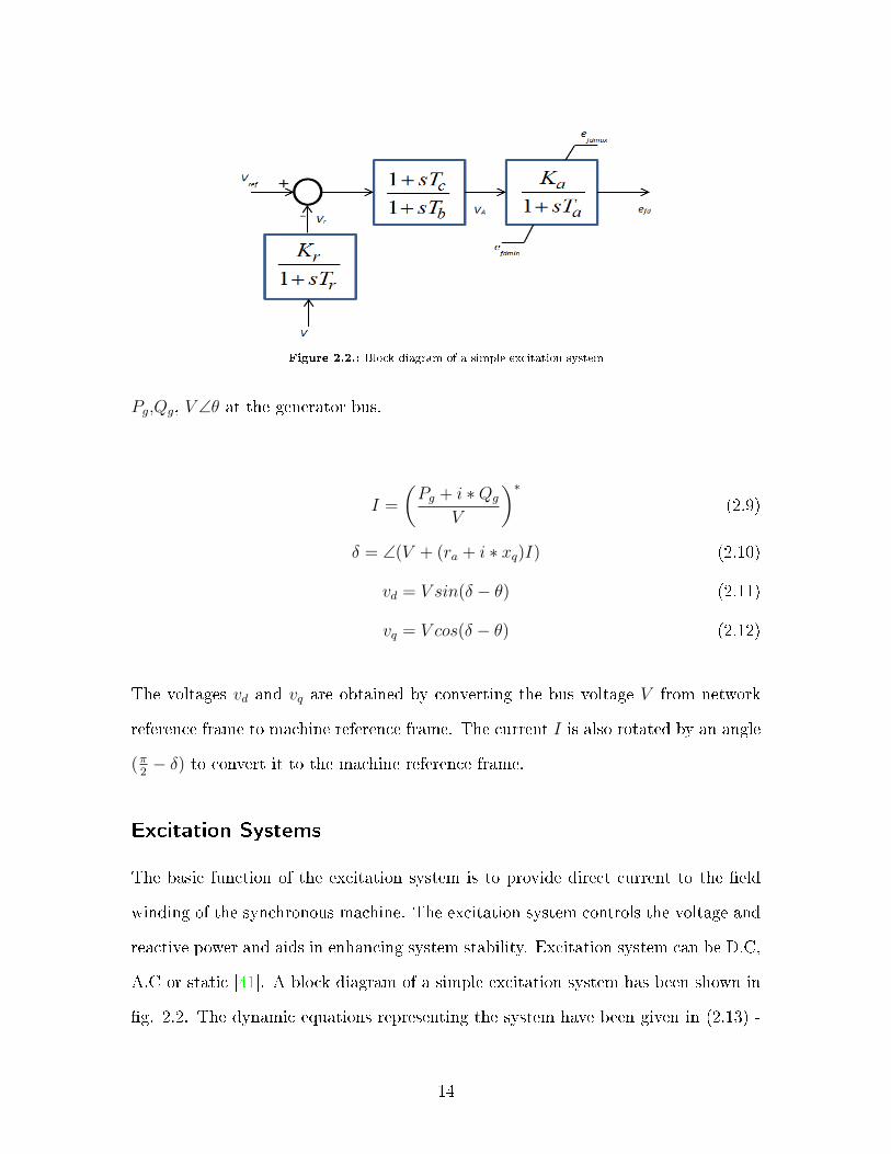
Figure 2.2.: Block diagram of a simple excitation system

Pg,Qg, V ∠θ at the generator bus.

I =

(Pg + i ∗Qg

V

)∗(2.9)

δ = ∠(V + (ra + i ∗ xq)I) (2.10)

vd = V sin(δ − θ) (2.11)

vq = V cos(δ − θ) (2.12)

The voltages vd and vq are obtained by converting the bus voltage V from network

reference frame to machine reference frame. The current I is also rotated by an angle

(π2− δ) to convert it to the machine reference frame.

Excitation Systems

The basic function of the excitation system is to provide direct current to the eld

winding of the synchronous machine. The excitation system controls the voltage and

reactive power and aids in enhancing system stability. Excitation system can be D.C,

A.C or static [41]. A block diagram of a simple excitation system has been shown in

g. 2.2. The dynamic equations representing the system have been given in (2.13) -

14

(2.15).

Vr =(KrV − Vr)

Tr(2.13)

Vas =

((1− Tc

Tb

)(Vref − Vr)− Vas

)/Tb (2.14)

efd =(KaVA − efd)

Ta(2.15)

where Vas is the internal state variable associated with the lead-lag block.

Governor

The governor has the responsibility to control the power output of the synchronous

machine and thus the frequency. The droop controls the amount of change in power

with change in frequency. The purpose of droop is to enable parallel operation of

multiple generators. The time constants associated with governor controls are small

and are slow acting. Governor is used for relatively slower control actions such as

automatic generation control (AGC). The block diagram of a simple governor has

been shown in g. 2.3. The dynamic equations associated with the governor have

been given in (2.16) (2.18).

xg1 =(Pin − xg1)

T1

(2.16)

xg2 =

((1− T3

T2

)xg1 − xg2

)/T2 (2.17)

xg3 =

((1− T5

T4

)(xg2 +

T3

T2

xg1

)− xg3

)/T4 (2.18)

where xg1, xg2 and xg3are the internal state variables of the governor control blocks.

15

Figure 2.3.: Block diagram of a simple governor-turbine system

Figure 2.4.: Block diagram of a PSS

Power System Stabilizer (PSS)

The main purpose of PSS is to add a supplementary damping signal to the excitation

system. PSS uses feedback signals such as generator speed, generator power or gen-

erator acceleration to produce the supplementary signal. PSS produces a damping

torque in phase with the rotor speed deviations in order to aid in oscillation damping.

The basic block diagram of PSS has been shown in g. 2.4.

The dynamic equations associated with the PSS are given in (2.19) - (2.21)

v1 =(Pin − xg1)

T1

(2.19)

v2 =

((1− T3

T2

)(KPSS∆ω + v1)− v2

)/T2 (2.20)

v3 =

((1− T5

T4

)(v2 +

(T3

T2

(KPSS∆ω + v1)

))− v3

)/T4 (2.21)

16

Figure 2.5.: Block diagram of a SVC

Static VAR Compensator (SVC)

A SVC is a shunt FACTS device that injects reactive power at the point of connection.

It is mainly used to support voltages in the system. It can also be utilized for damping

inter-area oscillations by providing a supplementary signal to the voltage reference

through a supplementary control loop. The basic block diagram of PSS has been

shown in g. 2.5.

Bcon =

((1− Tc

Tb

)(Vref + ∆Vsup − V )−Bcon

)/Tb (2.22)

Bsvc =(KrBcv −Bsvc)

Tr(2.23)

whereBconis the internal state variable of the lead-lag block. ∆Vsup is the signal that

comes from a supplementary control loop to enable SVC to participate in damping

of oscillations.

2.2. Small Signal Stability and Linearized Model of

a Power System

As mentioned earlier, a power system is a highly interconnected dynamic system.

In order to analyze the stability of this system as a whole, a non-linear dierential

17

algebraic model is obtained by combining the dierential equations of various com-

ponents enlisted in the previous section and the algebraic equations associated with

the network [41]. The dierential algebraic equations of the power system have been

given in (2.24) - (2.26) [40].

x = f(x, xa, u) (2.24)

0 = g(x, xa, u) (2.25)

y = h(x, xa, u) (2.26)

where x are the state variables of the system, xa is the vector of algebraic variables,

u is a vector of input variables, f is a vector of dierential equations, g is a vector of

algebraic equations, h is a vector of output equations and y is the output vector of

the system. Small signal stability deals with the analysis of equilibrium points where

˙x = 0. The primary step towards small signal analysis is to determine the state space

matrices of the power system around an equilibrium point. The equilibrium point is

obtained by running a load ow of the system. Following load ow, there are two

methods to obtain the state space matrices of the system around an equilibrium point:

1) Using analytic jacobian.

2) Numerical approximation.

The modeling and control implementation presented in this dissertation have been

carried out in a MATLAB based toolbox called power system toolbox (PST) [42]. PST

uses the numerical perturbation approach for obtaining the state space matrices. A

partitioned explicit approach is used where the dierential and algebraic variables are

updated separately [43]. The method involves perturbing the variable x and u and

obtaining the matrices ∆f∆x, ∆f

∆u, ∆h

∆x, ∆h

∆u. Thus the state space representation of the

system is given as:

18

x = Ax+Bu (2.27)

y = Cx+Du (2.28)

where A ∈ Rn×n, B∈Rn×m, C ∈ Rr×n and D ∈ Rr×m is the output vector. The

matrix D is always a zero matrix since the transfer functions associated with dierent

dynamic components of a power system are proper. Once the linearized model of the

power system is obtained, its stability and response around that operating point is

governed by the eigenvalues. The n eigenvalues of the system can be determined by

nding the roots of the characteristic equation given in (2.29).

det(A− λiI) = 0 (2.29)

where In×n is an identity matrix. The eigenvalues can be represented as σi ± jκi

where κi = 0 for purely real ones and σi = 0 for purely imaginary ones. The system

is stable i all σi ≤ 0. Two important parameters associated with any eigenvalue are

the damping, ζi and frequency, fi of that eigenvalue. These are given as:

ζi =−σi√σ2i + κ2

i

(2.30)

f =κi2π

(2.31)

The right and left eigenvectors, vi and ui, are determined using (2.32) and (2.33)

respectively.

19

Avi = λivi (2.32)

wiA = wiλi (2.33)

The signicance of right eigenvector is that its elements indicate the relative activity

of a state variable in a mode whereas the elements of left eigenvector indicate the

contribution of a state variable to a mode. In order to normalize the relationship

between state variables and modes, a matrix called as participation matrix P is dened

[41]. The ith column of P has been shown in (2.34).

pi =

p1i

p2i

.

.

pni

=

v1iwi1

v2iwi2

.

.

vniwin

(2.34)

Electromechanical modes are the system modes associated with machine rotor state

variables (angle and speed). As mentioned in chapter 1, electromechanical modes

normally lie in the low frequency range ranging from 0.2 Hz to 2.5 Hz. The elec-

tromechanical modes that have a high participation in a specic machine's rotor

state variables (angle and speed) are the local modes associated with that machine.

On the other hand, an inter-area mode involves multiple machine rotor state vari-

ables participating in it. Participation factor analysis aids in choosing the location of

installing a controller in case an electromechanical mode is poorly damped.

The poorly damped electromechanical modes in the system are known as the critical

modes. This dissertation specically involves the study and control of critical inter-

20

area modes. Using the analysis presented till now, the main challenges associated

with the damping of inter-area modes are that:

1) In a large power system, since multiple machines participate in inter-area modes,

usually there is no one location where a local controller can alleviate the problem.

2) In a stressed operating condition, even a small disturbance can make them

migrate into the right half plane or in other words make the system unstable.

Therefore, a centralized WAC has been proposed in the literature and implemented

in this work for enhancing the damping of critical inter-area modes. The rapid de-

velopment in phasor measurement technology has made possible the use of remote

feedback signals for control. A generic schematic of a WAC has been shown in g.

2.6. It is worth noting that the WAC can be either designed as a state feedback or an

output feedback controller. However, since the number of state variables in a realistic

power system is large, state feedback controller is not a feasible choice. Therefore,

this dissertation studies and implements an output feedback WAC and that is what

has been shown in g. 2.6.

The rst step towards designing the WAC involves selecting appropriate I/O signals

such that inter-area modes are controllable/observable. The participation factor does

not link the system modes to system input and outputs (only depends on the state

matrix). Therefore, the residue method has been used in this work [24]. Residue

provides a combined metric of controllability and observability of a mode using the

chosen I/O signals. The transfer function G(s) of the power system can be written

in terms of the residues as:

G(s) =y(s)

u(s)=

n∑i=1

Ri

s− λi(2.35)

where,

21

Figure 2.6.: Schematic of a WAC

Ri = ||CviuTi B|| (2.36)

The residue Ri for the ith mode is also the sensitivity of that mode to a general

feedback gain K or in other words, the impact that a small change in a proportional

feedback gain K will have on the eigenvalue λi.

Therefore, in g. 2.6, the signals u1,sup,...,um,sup are supplementary signals provided

by the WAC. The user selects the dimension m and r by choosing the signals that

enable control of the critical inter-area mode. Once, the appropriate I/O signals are

selected, the next step is to design the controller that improves the damping of the

critical inter-area mode/s without impacting the rest of the modes in a negative way.

The rest of the dissertation targets the design of a WAC for enhancing the damping

of critical inter-area modes using eigenstructure assignment.

22

3.Design of a Wide Area Controller

This chapter demonstrates the application of partial right eigenstructure assignment

for designing an output-feedback based WAC in a power system. The unique feature

of the controller is that it utilizes the additional design freedom provided by right

eigenvectors along with eigenvalue placement to improve the dynamic behavior of the

system. The fact that multi-input-multi-output (MIMO) systems provide more design

freedom than just manipulating the eigenvalues of the system has been exploited for

controller design. Supplementary loops on two static VAR compensators (SVC) have

been utilized to achieve the damping of oscillations. The advantage of using SVC

(or any other FACTS devices) is that it is better suited for damping of inter-area

oscillations since it is installed directly on the tie-line and it ensures low interaction

with the local electromechanical modes of the system. A very important aspect of

designing a WAC is its robustness against time delay of feedback signals. This chapter

also presents a multi-model optimization strategy to deal with uncertainty in time

delays.

A number of existing techniques involve coordinating the decentralized controllers

(PSSs, FACTS PODs) in the system using optimization techniques such that all the

eigenvalues of the system follow the minimum damping criterion (normally set to be

5%) [9], [44], [45] . These methods are based on moving poorly damped poles to well

damped locations. However, it is a well-known fact that the transient response of a

system is governed by not only the eigenvalues but also the eigenvectors. In [34], it

was rst shown that MIMO systems provide more design freedom than assignment of

eigenvalues for the case of state feedback. In [36], the necessary and sucient condi-

tions for exploiting additional degrees of freedom on top of assigning the eigenvalues

23

was presented for the case of output feedback. Depending upon the number of inputs

and outputs of the MIMO systems, a limited number of eigenvalues and associated

right or left eigenvector can be appropriately assigned. In a typical power system,

there are only a few inter-area modes that are of concern. Therefore, eigenstructure

assignment forms a suitable technique to assign these critical inter-area modes along

with the corresponding right eigenvectors. Feedback signal selection plays an impor-

tant role to ensure that the critical inter-area modes are controllable (have a good I/O

controllability metric/residue) while the local modes have a low I/O controllability

metric.

This chapter presents the design of a hierarchical, WAC that operates on top of

local controllers in order to damp inter-area oscillations. The unique feature of the

algorithm is that it formulates the controller design problem as a quadratic optimiza-

tion problem which can be solved in a single step (being a convex problem) [46, 47].

Unlike [38], a transfer function representation of the dynamic compensator has been

used where the numerator coecients of the elements of the compensator form the

optimizing variables. The denominator poles as well as closed-loop right eigenvectors

corresponding to the inter-area modes have to be pre-assigned in order to formulate

the controller design problem as a quadratic optimization problem. For this purpose,

a SVD based technique is used to determine the basis vectors for each achievable

(or assignable) closed-loop right eigenvector [46]. This is followed by determining

the weights to be used with these basis vectors to obtain the closed-loop right eigen-

vectors using projection techniques [48, 49] . Two projection techniques utilizing

open-loop right eigenvector projection and weighted open-loop eigenvector projection

using participation factors of the state variables in the inter-area modes have been

employed and compared. Reference [49] has shown that utilization of open-loop right

eigenvector projection to obtain the closed-loop right eigenvector results in a robust

24

closed-loop system (small condition number of the closed loop modal matrix). It has

to be noted that although the system under study already consists of local controllers,

it is still considered as an open-loop for the purpose of eigenvector projection since a

hierarchical control structure has been adopted.

An important aspect involved in the design of a WAC is the time delay of feedback

signals. In [50, 51], it has been shown that communication latency or time delay of

feedback signals degrades the performance of the controller. Design of a WAC con-

sidering time delays has been addressed using robust control techniques [52], incor-

poration of time delay into system model using Pade approximation [32] and using

delay-dependent stability analysis [53]. In [54], a mu synthesis approach has been

used to design a robust controller with time delay as an uncertain parameter. In this

chapter, a multi-model optimization problem based on partial right eigenstructure

assignment has been formulated to design a WAC robust to uncertain time delays.

Pade approximation has been used to approximate the time delay as a rational trans-

fer function [32].

3.1. Controller Design Using Quadratic

Programming

Partial Right Eigenstructure Assignment

Consider the linearized model of a power system around an operating point as:

x = Ax+Bu (3.1)

y = Cx+Du (3.2)

25

where x∈Rn×1 is the state vector, u∈Rm×1 and y ∈ Rr×1 is the output vector. The

free response of the system from an initial state without any inputs is given as:

xi(t) =n∑i=1

vjicjeλjt (3.3)

cj =n∑k=1

wjkxk(0) (3.4)

where vi, wi are the right and left eigenvectors of eigenvalue λi respectively and x(0)

is the initial state vector. Therefore, the eigenvalues control the rate of decay whereas

the right eigenvector determines the shape of response.

The elements of right eigenvector determine the relationship between the state

variables and the associated mode. For a MIMO system, a few selected eigenvalues

and eigenvectors can be appropriately manipulated in order to improve the dynamic

performance of the system. In the case of proportional feedback, partial right eigen-

structure assignment technique is capable of assigning r eigenvalues and corresponding

r eigenvectors [38]. Let a proportional output feedback controller, u = Ky, be con-

nected to the system in (3.1) and (3.2). This results in the closed-loop state matrix

being (A + BKC). Assume i = 1...q ≤ r controllable eigenvalues are to be assigned

to locations λi . Then, the closed loop system has to satisfy (3.5).

(A+BKC)vi = λivi (3.5)

where vi ∈ C(n)×1 is the corresponding closed-loop right eigenvector. The problem of

eigenstructure assignment can be presented as the determination of controller K that

achieves the assignment of λi and vi. Once the location of λi is selected, the next step

is to determine vi that can be assigned. Unlike a SISO system, a MIMO system

can have multiple options for selecting a right eigenvector associated to an

26

eigenvalue. The equation (3.5) can be restructured into equations (3.6) and (3.7)

shown below.

[A− λiI B

] vi

fi

= 0 (3.6)

where, KCvi = fi (3.7)

The vector fi ∈ Cm×1 is known as the input-direction. It should be noted that the

eigenvector, vi, to be assigned cannot be chosen arbitrarily. It can be inferred from

(5) that the achievable vector

[vi fi

]Tcan only belong to the null-space of the

matrix

[A− λiI B

]. In other words, the achievable

[vi fi

]Tcorresponding

to an eigenvalue is some linear combination of the basis vectors of the null space of

matrix

[A− λiI B

]. The rank of this null-space is the same as the dimension of B.

Therefore, higher the dimension of B, the more is the degree of freedom available for

eigenvector assignment. Singular value decomposition (SVD) is used to determine the

null space of

[A− λiI B

]and obtain the basis vectors for the achievable closed-

loop right eigenvector. The right singular matrix can be split into sub-matrices as

given in (3.8).

Z =

Z11 Z12

Z21 Z22

(3.8)

The columns of Z12∈Cn×m form the basis vectors for achievable vi and columns of

Z22∈Cm×m form the basis vectors for the achievable fi. Let ηi∈ Cm×1 be the weights

to be used with the basis vectors to obtain the achievable

[vi fi

]T. The vector ηi

can be determined by projecting a desired eigenvector vd onto the subspace spanned

by the columns of as shown in (3.9) [55].

27

ηi =(ZT

12Z12

)−1ZT

12vd (3.9)

Then the achievable vi and fi are obtained as shown in (3.10).

vi = Z12ηi, fi = Z22ηi, (3.10)

Traditionally in power systems, vd is selected such that the participation of certain

machine speeds in inter-area modes is reduced [37,38]. Here two options of obtaining

ηi have been compared:

1) ηi =(ZT

12Z12

)−1ZT

12vi,ol where vi,ol is the open-loop right eigenvector.

2) ηi =(ZT

12PZ12

)−1ZT

12Pvi,ol where P is a diagonal matrix consisting of the par-

ticipation factors of mode i.

The elements of the right eigenvector determine the impact on respective system

state variables if the corresponding mode is excited. Thus, the aim of using open loop

right eigenvector projection is to avoid a drastic change in the dynamic behavior of

system when closing the feedback loop. This projection technique is also known to

result in robust design and small control gains [49]. The second projection technique

scales the open-loop right eigenvector by the participation factor. The logic behind

this approach is that all the state variables do not participate equally in a mode.

Therefore, weights are introduced in the projection problem of (3.9) by utilizing the

participation factor of the respective mode. Results using both the options will be

presented and compared.

Once vi and fi are determined, the feedback gain required for assignment of eigen-

value/eigenvector pairs can be obtained using (3.7) and is given in (3.11):

28

K =

[f1 . . . fq

] (LTL

)−1LT (3.11)

where L = C

[v1 . . . vq

].

Dynamic Compensator

Previous section dealt with partial right eigenstructure assignment for the case of

proportional feedback. However, since this work uses a dynamic compensator, new

necessary and sucient conditions have to be enlisted. The dynamic extension causes

the state space of the closed-loop system to belong to R(n+na)×1 where xc ∈ Rna×1 are

the state variables added by the compensator. Therefore, the closed-loop right eigen-

vector can be expressed as

[vi vci

]where vi represents the right sub-eigenvector

belonging to Cn and vci represents the right sub-eigenvector belonging to Cna . The

main reason for utilizing a dynamic compensator is that it increases the number of

eigenvalues and eigenvectors that can be assigned to r + na [38].

An important result used in this paper is that even though the dynamic order of the

closed-loop system increases to r + na, the assignment problem still depends on the

right sub-eigenvector vi [47]. Let's assume that the compensator in the state space

form is represented by matrices (Ac, Bc, Cc, Dc). The controller transfer function is

shown in (3.12).

K(s) = Cc(sI − Ac)−1Bc +Dc (3.12)

The closed-loop state space matrix obtained by applying (Ac, Bc, Cc, Dc) on the sys-

tem given in (3.1) and (3.2) is given in (3.13).

29

Acl =

A+BDcC BCc

BcC Ac

(3.13)

where Ac ∈ Rna×na , Bc ∈ Rna×r, Cc ∈ Rm×na , Dc ∈ Rm×r. Let's assume that the

closed-loop eigenvalues are represented by λi,cl. Then Acl has to satisfy (3.14). A+BDcC BCc

BcC Ac

vi

vci

= λi,cl

vi

vci

(3.14)

This matrix representation can be split into two equations given in (3.15) and (3.16).

(A+BDcC)vi +BCcvci = λi,clvi (3.15)

(BCc)vi + Acvci = λi,clvci ⇒ vci = (λi,clI − Ac)−1BcCvi (3.16)

Substitution of vci obtained in (3.16) into (3.15) results in the relationship shown in

(3.17).

(A+BDcC +BCc(λi,clI − Ac)−1BcC)vi = λi,clvi (3.17)

Utilization of (3.12) in (3.17) results in (3.18).

(A+BK(λi,cl)C)vi = λi,clvi (3.18)

The above relationship proves that even though the compensator adds some state

variables to the system, the assignment still depends on the rst n elements (vi) of the

closed-loop right eigenvector. In other words, (3.7) still holds with the exception that

K is replaced by K(λi,cl) . This is an important result that is used in the formulation

30

of the eigenstructure assignment problem in later sections. An eigenvalue/eigenvector

pair (λi,cl, vi) can be assigned by dynamic feedback K(s) i (3.19) is satised.

K(λi,cl)Cvi = fi (3.19)

If λi,cl is a complex eigenvalue (as will be in the case of an inter-area mode), a similar

constraint corresponding to complex conjugates (λi,cl, vi, fi) has to be satised.

Quadratic Programming

The design objectives of partial right eigenstructure assignment comprise of assign-

ing some critical eigenvalues and corresponding closed-loop right eigenvectors using

(3.6) - (3.10). Then (3.19) and its conjugate equivalent are the constraints that the

gain has to satisfy in order to assign the complex eigenvalue/eigenvector pair. Fur-

thermore, bounds can be imposed on the numerator coecients. Thus a quadratic

programming based optimization is formulated utilizing the dynamic compensator.

This paper uses a transfer function representation of the dynamic compensator. The

quadratic programming formulation is made possible by specifying the denominator

coecients of the compensator a priori. Thus, the optimization variables are the

numerator coecients. The degree of the numerator determines the number of op-

timizing variables in the system. If the algorithm does not converge with a specic

order of the numerator, the order can be increased with the constraint that the degree

of numerator cannot be greater than the denominator. A general kth order dynamic

compensator matrix is given in (3.20).

31

b111sk+.....+b(k+1)11

sk+a111sk−1+.....+ak11. . .

b11rsk+.....+b(k+1)1r

sk+a11rsk−1+.....+ak1r

. . . . . . . . .

. . . . . . . . .

b1m1sk+.....+b(k+1)m1

sk+a1m1sk−1+.....+akm1. . .

b1mrsk−1+.....+b(k+1)mr

sk+a1mrsk−1+.....+akmr

(3.20)

where b1mr.....b(k+1)mr represent the numerator coecients and a1mr.....akmr represent

the denominator coecients of the element (m, r) of the compensator. The constraint

(3.19) is made linear by pre-assigning the pair (vi, fi) using projection methods al-

ready presented. The optimization problem can be stated as shown below [47,56].

Quadratic cost function: The cost function consists of minimizing the sum of Frobe-

nius norm of the compensator at l dierent frequencies typically around the eigenval-

ues to be shifted as shown in (3.21). This norm of the controller at a given frequency

signies the amount of energy required for the control action at that particular fre-

quency [44,57]. Therefore, minimizing J ensures reduction in average control energy

over frequencies i = 1....l and it can be expressed as a quadratic function in terms of

the optimizing variables (numerator coecients).

Minimize J =l∑

i=1

||K(jωi)||2F (3.21)

Equality constraints : For i = 1....q complex eigenvalue/eigenvector assignments, the

2q equality constraints are given in (3.22) and (3.23).

K(λi,cl)Cvi = fi (3.22)

K(λi,cl)Cvi = fi (3.23)

Numerator coecient bounds : The supplementary control signals from the controller

32

are dependent on the magnitude of the feedback. Therefore, it is necessary to put

a bound on the elements of the feedback matrix in order to limit the control eort.

The optimization variables, i.e., numerator coecients can be bounded as shown in

(3.24).

bmin ≤ bijk ≤ bmax (3.24)

Once the cost function and the equality constraints are obtained in terms of the nu-

merator coecients, quadratic programming is used in MATLAB to solve the prob-

lem. The formation of all the matrices that are required to be fed to quadprog can be

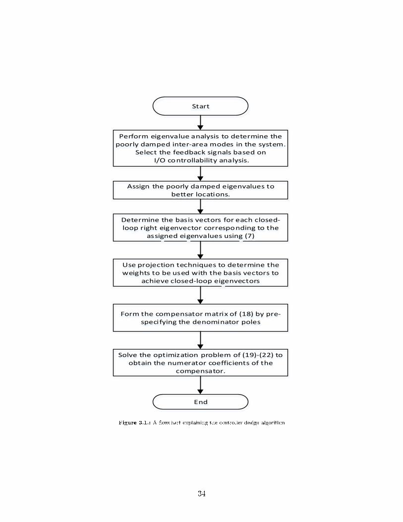
found out in detail in [58]. A owchart explaining the algorithm for controller design

using partial right eigenstructure assignment has been shown in g. 3.1.

3.2. I/O Signal Selection and Time Delay of

Feedback Signals

Selection of appropriate I/O signals for the controller is important to ensure that all

the poorly damped modes to be relocated are controllable and observable. Poor choice

of signals might result in unreasonably high gains and thus an infeasible controller.

In this work, the locations of SVCs have been pre-assigned. The SVCs are installed

close to the tie lines which is the followed practice in an actual power system. The

challenge here is to select the appropriate feedback signals given the locations of SVCs

are xed. The residual method explained briey in chapter 2 is used for selecting the

feedback signals for the WAC. As was mentioned earlier, the residual method also

represents the rst order sensitivity of an open-loop eigenvalue λi,ol with respect to a

controller K. The metric based on the rst order perturbation of an eigenvalue has

been used and given in (3.25) [59,60].

33

!"

#$ %

&&

' ( )*"

+ )," --"

.

Figure 3.1.: A owchart explaining the controller design algorithm

34

dλi,oldK

= ||CviuTi B|| (3.25)

The primary reason for using SVCs is to ensure that the local modes in the system

are minimally aected. On the other hand if PSS/s were chosen to be a part of the

WAC scheme, the control interaction might result in a local mode becoming unstable

or moving towards the right half plane as the inter-area modes are moved to better

locations. As will be shown in the results, utilizing SVCs and the selected feedback

signals results in the local modes being non-controllable. Also, the modes other than

the inter-area modes that are controllable using the chosen I/O signals are well into

the left half plane. This is the reason that no constraint is put on the other eigenvalues

(other than the assigned ones) in the optimization process to ensure that none of them

becomes unstable.

An important factor while using remote feedback signals is to account for the time

delay. Time delay has been approximated by utilizing the second order Pade approx-

imation as given in (3.26) [32].

e−τs =τ 2s2 − 6τs+ 12

τ 2s2 + 6τs+ 12(3.26)

The state space representation of the dynamics of delay can be written as shown in

(3.27) and (3.28). The time delay block connected to the plant has been shown in

g. 3.2.

xd = Adxd +Bdud (3.27)

y1d = Cdxd +Ddud (3.28)

where y1d is one of the delayed outputs of the plant. A similar representation can

be used for other inputs. The input ud to the time delay block is one of the outputs

35

Figure 3.2.: time delay in one of the output signals

from the plant. Thus ud can be substituted with y1 using (3.2). The nal state space

representation of the system including the time delay can be written as given in (3.29)

and (3.30).

˙xtd = Atdxtd +Btdutd (3.29)

ytd = Ctdxtd +Dtdutd (3.30)

where xtd =

x

xd

, ytd =

y1d

y2

, Atd =

A 0

BdCr1 Ad

, Btd =

B

BdDr1

,Ctd =

DdCr1 Cd

Cr2 0

, Dtd =

DdDr1

Dr2

. Cr1, Cr2, Dr1 and Dr2 represent the

respective rows of C and D matrices.

The impact of time delay on the performance of a WAC employing remote signals

has been presented in numerous works [29, 50]. Local control typically experiences

time delay of the order of 10ms. However, in a wide area control scheme, the remote

signals might have a delay of the order of 100ms. If a larger number of signals are to

be routed, a delay of more than 100ms is expected. Moreover, transmitting multiple

signals introduces variability in the amount of time delay. Therefore, accounting for

36

an uncertain time delay is very important to ensure that the controller is robust to

uncertainty in time delay. A multi-model optimization approach has been followed

to incorporate the impact of time delay and has been presented in the next section.

3.3. Multi-model Optimization for Controller

Design

As mentioned in the previous section, time delays of feedback signals degrade the

performance of a WAC. A constant time delay can be accounted into controller design

by using a lead-lag compensation block [53]. However, the challenge is the uncertainty

in time delay. In a recent work, a mu-synthesis based approach has been used where

the time delay has been considered as an uncertain parameter for determining the

linear fractional transformation of the system [54]. This work proposes to use a

modal multi-model method for incorporating the uncertainty in time delay into the

controller design. A quadratic optimization problem utilizing the system model with

and without the time delay is setup. The time delay is included in the system model

by using (3.26) - (3.30). A specic value of time delay, τ , is chosen and the design

algorithm results in a controller that is robust to multiple values of time delays up to

τ . Let's assume that the system model with and without the delay is termed as the

delayed model and the nominal model respectively. The multi-model optimization

problem formulation will be presented below.

Let the controller designed for the nominal model be termed as Knom(s). The

aim is to design a controller, Krobust(s), that ensures the damping of the inter-area

modes for the varying values of time delay of feedback signals. Let λi1,cl be the

i1 eigenvalues that were assigned by Knom(s) for the nominal model. Also, assume

37

that the nominal and delayed system models are represented as (A1, B1, C1, 0) and

(A2, B2, C2, 0) respectively. The steps for robust controller design are listed below:

• Apply the controller, Knom(s) on the delayed system model. Determine the

eigenvalues that violate the minimum damping criteria (5% damping).

• The design objective for Krobust(s) is to assign the eigenvalues obtained from

the previous step to better locations, λi2,cl, while preserving the eigenvalues,

λi1,cl, assigned by Knom(s) for the nominal model. The optimization problem

involving the assignment of (λi1,cl, vi1, fi1) and (λi2,cl, vi2, fi2) for the nominal

and the delayed system model respectively is shown in (3.31) - (3.34) [61].

Minimize J =l∑

i=1

||Knom(jωi)−Krobust(jωi)||2F (3.31)

such that,

Krobust(λi1,cl)C1vi1 = fi1 (3.32)

Krobust(λi2,cl)C2vi2 = fi2 (3.33)

bmin ≤ bijk ≤ bmax (3.34)

where λi1 = 1...q1 ≤ r + na, λi2 = 1...q2 ≤ r + na. The objective function in (27)

ensures that the controller Krobust(s) is as close as possible to Knom(s) [58]. Also, the

objective function can be expressed as a quadratic function in terms of the numer-

ator coecients of Krobust(s). Therefore, the optimization is solved using quadratic

programming in MATLAB. The matrices required for quadratic programming for-

mulation have been given. There are two important factors to be considered while

38

incorporating multiple models for controller design using eigenstructure assignment:

1. Similar to sub-section 3.1.3, the constraints of (3.32) and (3.33) can be linearized

i (vi1, fi1) and (vi2, fi2) are pre-assigned. The equations (3.9) and (3.10) are

used to determine the vectors (vi1, fi1) and (vi2, fi2). The matrices required

for determination of these vectors are Z12 and vi,ol. Z12 for the two state space

models is obtained using null(

[A1 − λi1I B1

]) and null(

[A2 − λi2I B2

]).

The next important step is to select vi,ol. The eigenvalues being treated in this

subsection are the ones obtained by the application of Knom(s) on the nominal

and the delayed model. Therefore, the eigenvector vi,ol corresponding to these

eigenvalues belong to the space C(n+na)×1(application of Knom(s) increases the

dynamic order). This would result in the matrices Z12 and vi,ol needed in (3.9)

being dimensionally incompatible (Z12 ∈ Cn×m whereas vi,ol ∈ C(n+na)×1) .

This problem is solved by exploiting the concept presented in (3.12) - (3.18).

Therefore only the rst n elements of vi,ol are used for projection.

2. It is possible to have constraints treating the same type of mode in two dierent

models. This would result in high sensitivity of that eigenvalue and thus lower

robustness [61]. Care should be taken to remove a constraint for the nominal

model if a similar constraint is being added for the delayed model. This point

will also be demonstrated in the results section more clearly.

It has to be noted that the dynamic order of Knom(s) and Krobust(s) has been selected

to be the same in this work. However, the orders can be chosen to be dierent.

39

3.4. Results and Discussion

The algorithm presented in this chapter has been applied to the IEEE 68 bus system.

The system has been built and simulated in matlab based power system toolbox

(PST) [42]. A modied version of the system presented in [62] has been used. The

details of the system have been provided in appendix A. A schematic showing the

system with the WAC has been shown in g. 3.3. The system has two SVCs rated

200 MVA located at buses 40 and 50. The damping has been achieved by providing

a supplementary signal to the SVC reference voltage signals. The reason for using

two SVCs is to provide enough degrees of freedom for eigenvector assignment as

explained in section 3.1. The dynamic model of the system in PST consists of 186

state variables. Sixth order model has been used for synchronous machines and the

loads have been modeled as constant impedance loads. PSSs and governors have been

installed only on machines 1 12 considering the fact that the generators 13-16 are

equivalent areas.

Controller Design for the Nominal Model

The initial step consists of performing a small signal stability analysis on the nominal

model to determine the inter-area modes in the system. The next step involves

selecting the I/O signals that have a good controllability metric for the poorly damped

eigenvalues (damping ratio less than 5%). Since the output signal of the controller is

xed to be the SVC supplementary voltage control signal, the aim is just to nd the

appropriate input signals. The feedback signals based on the controllability metric

were chosen to be the real power ows in the lines 49-52 and 52-42. The selection

of these feedback signals also ensured that none of the local modes were controllable.

The other possible options for tie lines (42-41, 50-52) were also successfully used for

40

controller design but the results have not been presented here due to limited space.

The I/O controllability of the top ten controllable modes using the selected I/O signals

has been presented in table I. It can be observed that except the inter-area modes,

majority of the other controllable modes have a high, negative real part. The next

step is to choose the locations to be assigned to the poorly damped eigenvalues. The

approach followed here is to keep the imaginary part the same and change the real part

such that the damping ratio becomes 10%. It has been noted that the damping ratio

of the eigenvalue −0.308 ± 2.392i is already above the minimum damping criterion.

Therefore, it is assigned at the same location. The open-loop and assigned eigenvalues

have been shown in table II.

Figure 3.3.: IEEE 68 bus system with the WAC

41

Table 3.1.: Residues of top 10 controllable eigenvalues using the selected I/O signals

Open-loop eigenvalues Residues

-61.66 21.8-68.73 6.63-67.77 2.78

-0.117+3.329i 2.2-0.178+4.889i 1.19-0.308+2.392i 1.17-9.05+11.61i 1.14

-28.67 0.64-7.59+19.73i 0.53-7.95+14.86i 0.43

Table 3.2.: Assigned eigenvalues and their damping ratios

Open-loop eigenvalues Closed-loop eigenvalues Open-loopdampingratio

Closed-loop

dampingratio

-0.308+2.392i -0.308+2.392i 12.8% 12.8%-0.117+3.329i -0.334+3.329i 3.54% 10%-0.178+4.889i -0.491+4.889i 3.65% 10%

The achievable closed-loop right eigenvectors corresponding to each eigenvalue are

determined using (3.9) and (3.10) using either of the eigenvector projection techniques

mentioned in section 3.1. Once, the closed-loop right eigenvectors are determined,

the optimization problem utilizing equations (3.21) - (3.24) is setup. The order of the

dynamic compensator is chosen to be three and the compensator poles are chosen to

be (−4,−5,−6). It has to be noted that the controllability metric dened in (3.25)

is based on a proportional output feedback. However, using a dynamic compensator

adds new poles into the system. The location of these poles will have a marginal

eect on some of the system eigenvalues. Therefore, the closed-loop system eigenvalue

plot will have a few other eigenvalues displaced marginally than expected from the

controllability metric of table I. Choice of complex compensator poles has the least

42

impact on other system eigenvalues and is the best choice. It has to be noted that

these system eigenvalues being marginally displaced are the ones that lie into the far

left half plane. The local modes were not aected at all in any of the cases that

were studied. The degree of numerator has been chosen to be equal to that of the

denominator. The cost function is formulated to minimize the sum of the Frobenius

norm of the compensator at frequencies ranging from 0 to 7 rad/s in increments of

1 rad/s. The numerator coecients in the optimization problem are bounded to

be within -120 and 120. In this paper, both the projection techniques presented in

section 3.1 have been used for designing the controller. The controllers designed using

open-loop eigenvector projection and weighted open-loop eigenvector projection are

termed as Knom1(s) and Knom2(s) respectively. The performance of Knom2(s) is found

out to be superior to Knom1(s). Thus, Knom2(s) is used for the design of Krobust(s)

presented in the next subsection. The controllers Knom1(s) and Knom2(s) are found

to be [63]:

Knom1(s) =

−0.327s3+2.847s2−11.454s−36.123s3+15s2+74s+120

1.181s3+6.82s2+12.27s+59.956s3+15s2+74s+120

0.118s3−1.417s2+2.723s+14.5s3+15s2+74s+120

0.441s3−0.24s2+2.371s−12.85s3+15s2+74s+120

(3.35)

Knom2(s) =

0.0818s3+0.890s2−1.265s−36.44s3+15s2+74s+120

0.215s3−0.211s2−1.671s−33.98s3+15s2+74s+120

0.420s3+3.843s2+3.193s+37.41s3+15s2+74s+120

1.075s+9.169s2+10.77s+62.62s3+15s2+74s+120

(3.36)

The eigenvalues of the system with and without the output feedback controller have

been shown in g. 3.4. Fig. 3.4 shows that the controller selectively assigns the

poorly damped modes to better locations while preserving the well damped inter-area

mode at the same location. Furthermore, the rest of the eigenvalues are minimally

impacted. The time domain results have been shown for three dierent operating

43

conditions to justify the inherent robustness of the controller as shown in table III.

The operating condition, OP1, is the base-case condition. The operating condition,

OP2, involves increasing the output of generator 15 by 10 per unit (on 100 MW base)

while reducing the output of generator 14 by the same amount. This operating point

stresses the tie line 42−41 and worsens the damping of the eigenvalue of the nominal

system. The operating point, OP3, consists of the line 46− 49 being disconnected. A

ten cycle, three phase fault at bus 49 has been used to demonstrate the performance

of the controller under dierent operating conditions.

−3 −2.5 −2 −1.5 −1 −0.5 0 0.5 10

2

4

6

8

10

12

Real

Ima

gin

ary

Without controllerWith K

nom2(s)

modes of interest

5% damping line10% damping line

Figure 3.4.: IEEE 68 bus system with the WAC

Table 3.3.: Operating points used for validating the robustness of the controller

OperatingPoint

Operating Condition

OP1 base-caseOP2 increase the output of generator 15 by 10

p.u while reduce the output of generator 14by 10 p.u

OP3 line 46-49 disconnected

44

The plot showing the rotor angle dierence between generators 15 and 16 for dierent

faults and operating conditions have been shown in g. 3.5. The results clearly

indicate the signicance of eigenvector assignment in the design of the controller.

As seen from the results, Knom2(s) is more robust to operating point changes in the

system as compared to Knom1(s). Fig. 3.6 shows the susceptance of the SVCs during

fault for all the three operating conditions when using Knom2(s). This gure validates

that control objective is achieved with bounded control eort.

Multi-model optimization for controller design

Once the controller for the nominal system model, Knom2(s) is obtained, the next

step is to determine, the next step is to determine Krobust(s) robust to time delay

uncertainty of the feedback signals. The delayed system model is obtained by using a

value of τ = 400ms. The controller, Knom2(s), is applied to the delayed system. Two

eigenvalues, (−0.1073± 3.555i) and (−0.0436± 5.172i) are found to violate the min-

imum damping criterion. A multi-model optimization problem is formulated using

equations (3.31) - (3.34) to improve the damping of these eigenvalues while preserving

the performance of Knom2(s) for the nominal model. Ideally, the eigenvalues assigned

in the previous subsection are re-assigned at the same location to form the constraints

associated with the nominal model. Similarly, the eigenvalues (−0.1073±3.555i) and

(−0.0436±5.172i) associated with the delayed model are assigned to better locations

to form the constraints relative to the delayed system model. However, it has to be

noted that two eigenvalues associated with the delayed model are similar in nature to

the ones assigned for the nominal model. Therefore, the constraints associated with

the re-assignment of (−0.334±3.329i) and (−0.491±4.889i) at the same location are

removed for the nominal model. The utilization of the idea of eigenvector projection

45

ensures that the removal of these constraints does not aect these eigenvalues drasti-

cally while improving the damping of (−0.1073± 3.555i) and (−0.0436± 5.172i) for

the delayed model. The two poorly damped eigenvalues associated with the delayed

model are assigned to have a damping ratio of 7%. Similar to previous subsection,

this is achieved by keeping the imaginary part constant and varying the real part.

The assigned locations are found to be (−0.249± 3.555i) and (−0.362± 5.172i). The

eigenvalue plot showing the comparison of Knom2(s) and Krobust(s) on the nominal

and delayed system models has been shown in g. 3.7. Similar to previous subsection,

the numerator coecients in the optimization problem are bounded to be within -120

and 120. The controller Krobust(s) is given to be [63]:

Krobust(s) =

−1.411s3+10.039s2−21.75s+118.63s3+15s2+74s+120

2.274s3−2.47s2+22.57s−37.52s3+15s2+74s+120

−3.346s3−2.19s2−56.5s−61.72s3+15s2+74s+120

4.436s3+13.511s2+44.37s+98.53s3+15s2+74s+120

(3.37)

The eigenvalue plots presented in g. 3.7 show that the controller, Krobust(s) is able

to meet the minimum damping criterion for the nominal as well the delayed system

model. Two controller induced poles also come into the picture as shown in g.

3.7(b). However, they do not pose any problem as they are well into the left half

plane. Moreover, the local modes in both the eigenvalue plots are not aected at all.

46

0 2 4 6 8 10 12 14 16 18 200.1

0.15

0.2

0.25

0.3

0.35

time(s)

δ 15 −

δ1

6

Without WACWith K

nom1(s)

With Knom2

(s)

(a) Angle dierence for OP 1, fault at bus 49

0 2 4 6 8 10 12 14 16 18 200.4

0.45

0.5

0.55

0.6

0.65

time(s)

δ1

5 −

δ1

6

Without WACWith K

nom1(s)

With Knom2

(s)

(b) Angle dierence for OP 2, fault at bus 49

0 2 4 6 8 10 12 14 16 18 20

0.16

0.18

0.2

0.22

0.24

time(s)

δ1

5 −

δ1

6

Without WACWith K

nom1(s)

With Knom2

(s)

(c) Angle dierence for OP3, fault at bus 49

Figure 3.5.: Comparison of performance of Knom1(s) and Knom2(s)

47

0 2 4 6 8 10 12 14 16 18 20-2

-1.5

-1

-0.5

0

0.5

1

1.5

2

time (s)

SV

C s

ucep

tanc

e (1

00 M

VA

bas

e)

SVC at bus 40, OP1

SVC at bus 50, OP1

SVC at bus 40, OP2SVC at bus 50, OP2

SVC at bus 40, OP3

SVC at bus 50, OP3

Figure 3.6.: Susceptance of the SVCs during fault for all three operating conditions when using Knom2(s)

The Time domain results showing the rotor angle dierences between generators 15

and 16 for dierent values of time delay of feedback signals have been shown in gs.

3.8 - 3.10. The disturbance applied in the system is a ten cycle, three phase fault

at bus 49. It has to be noted that the results shown incorporate delay in both the

feedback signals. The results show the robustness of the controller, Krobust(s), to

varying values of time delays under dierent operating conditions.

48

−3 −2.5 −2 −1.5 −1 −0.5 0 0.5 10

2

4

6

8

10

12

Real

Ima

gin

ary

With Knom2

(s)

With Krobust

(s)5% damping line

(a) Comparison of eigenvalues with Knom2(s) and Krobust(s) connected to the nominal system

−3 −2.5 −2 −1.5 −1 −0.5 0 0.5 10

2

4

6

8

10

12

Real

Ima

gin

ary

With Knom2

(s)

With Krobust

(s)

controller induced poles

5% damping line

−0.362 + 5.172i

−0.249 + 3.555i

(b) Comparison of eigenvalues with Knom2(s) and Krobust(s) connected to the delayed system

Figure 3.7.: Comparison of the performance of Knom2(s) and Krobust(s) connected to the nominal and delayedsystem

49

0 2 4 6 8 10 12 14 16 18 200.12

0.14

0.16

0.18

0.2

0.22

0.24

0.26

0.28

time(s)

δ 15 −

δ1

6

With Knom2

(s)

With Krobust

(s)

(a) Angle dierence for OP 1 with a feedback delay of 200ms

0 2 4 6 8 10 12 14 16 18 200.12

0.14

0.16

0.18

0.2

0.22

0.24

0.26

0.28

time(s)

δ 15 −

δ1

6

With Knom2

(s)

With Krobust

(s)

(b) Angle dierence for OP 1 with a feedback delay of 400ms

Figure 3.8.: Comparison of the performance of Knom2(s) and Krobust(s) for OP1 and dierent values of timedelays

50

0 2 4 6 8 10 12 14 16 18 200.4

0.45

0.5

0.55

time(s)

δ 15 −

δ1

6

With Knom2

(s)

With Krobust

(s)

(a) Angle dierence for OP 2 with a feedback delay of 200ms

0 2 4 6 8 10 12 14 16 18 200.4

0.45

0.5

0.55

time(s)

δ 15 −

δ1

6

With Knom2

(s)

With Krobust

(s)

(b) Angle dierence for OP 2 with a feedback delay of 400ms

Figure 3.9.: Comparison of the performance of Knom2(s) and Krobust(s) for OP2 and dierent values of timedelays

51

0 2 4 6 8 10 12 14 16 18 20

0.16

0.18

0.2

0.22

0.24

time(s)

δ 15 −

δ1

6

With Knom2

(s)

With Krobust

(s)

(a) Angle dierence for OP 3 with a feedback delay of 200ms

0 2 4 6 8 10 12 14 16 18 20

0.16

0.18

0.2

0.22

0.24

time(s)

δ 15 −

δ1

6

With Knom2

(s)

With Krobust

(s)

(b) Angle dierence for OP 3 with a feedback delay of 400ms

Figure 3.10.: Comparison of the performance of Knom2(s) and Krobust(s) for OP3 and dierent values of timedelays

52

3.5. Discussion

There are certain aspects of the method that can be improved and have been addressed

in the next chapter. These are:

1. The method uses projection techniques to assign the closed-loop right eigenvec-

tors. However, the weights ηi to be used with the basis vectors can be used as

optimizing variables along with the eigenvalue locations since they are degrees

of freedom. This idea will be demonstrated in the next chapter to formulate

the controller design problem.

2. The controller was designed based on a linearized model around an operating

point. However, a power system experiences variability in operation throughout

the day. Therefore, robustness of the controller forms an important aspect.

In order to address this issue, a multi-model optimization formulation will be

presented in the next chapter. The multi-model optimization strategy presented

in this chapter is not particularly suited for scenarios where more than two

models are involved.

3. In the next chapter, a constraint on the damping of rest of the eigenvalues of

the system, other than the critical eigenvalues, will be incorporated.

53

4.Robustication of a Wide Area

Controller

One of the primary objectives of this thesis is to design a WAC that is robust to oper-

ating point changes in the system as well as time-delay uncertainties of the feedback

signals. As mentioned earlier, power systems experience varying operating conditions

throughout the day. Thus, robustness forms a very important aspect of designing a

WAC.

In control systems terminology, robustness can be subdivided into frequency domain

and real parametric uncertainties. There has been extensive research and literature

on addressing the issue of frequency domain uncertainty (mainly model uncertain-

ties) in power system using H-innity optimization technique [64]. The conventional

H-innity optimization technique involves selection of weighting lters to dene the

frequency range of interest for optimization which is not a very straightforward proce-

dure. A better method of nding the H-innity norm involves solving a linear matrix

inequality (LMI) where the eigenvalue constraints can be specied more easily [65].

On the other hand, the approach for addressing robustness against real parametric

uncertainties is totally dierent. Two dierent approaches have been used previ-

ously in power systems to design a controller robust to real parametric uncertainties

namely: µ synthesis (frequency domain) [66] and pole placement involving multiple

models of the system (time-domain) [45]. As the name suggests, robustness against

real parametric uncertainty involves studying the robustness of the system to any

variable parameter/s in the system. The µ-synthesis technique is a frequency domain

technique that uses a metric known as structured singular value (SSV) to analyze the

54

robust stability of the system. In [45], a pole placement technique has been presented

that uses a multi-model optimization approach with the tunable parameters of various

local controllers (PSSs) being the optimizing variables [45]. The control objective is to

ensure that eigenvalues across all the selected models satisfy the minimum damping

criterion.

This chapter presents formulation of multi-model optimization problems using two

dierent methods such that eigenvalues across all the selected models satisfy the

minimum damping criterion. This is achieved by tuning the initial controller K(s)

obtained using the technique presented in section 3.1. However, It should be noted

thatK(s) can be any generic WAC. The uniqueness of the tuning procedure lies in the

way the multi-model optimization problem is formulated. Two dierent approaches

have been used to select the models to be incorporated in the optimization problem:

1. Approach I - This approach involves selecting stressed operating points based

on system information. In power systems, these operating points are usually

known to the operator. A lot of existing literature follows this approach to

address the issue of robustness against operating point changes [39,45,67].

2. Approach II - The rst approach cannot address the issue of robustness of the

designed controller to the variation of a specic parameter of the system as well

as uncertain time delay of feedback signals. Approach II presents a method

to appropriately select models such that the resulting controller is robust to

uncertainties in operating points as well as time delays.

Two dierent methods have been used to setup the multi-model optimization problem

used in both the approaches:

1. Method 1 : This method is based on eigenstructure assignment technique. The

essence of the technique was explained in detail in the last chapter. However in

55

this chapter, the optimization problem is setup in a totally dierent way utilizing

a dierent set of optimizing variables as well as the optimization algorithm.

2. Method 2: This method makes use of the rst order sensitivity of an eigenvalue

with respect to a proportional feedback controller to slowly move the critical

eigenvalues associated with each of the selected models inside the 5% damping

line.

Both these methods will be explained in detail in the following sections.

The rst step towards tuning K(s) is to transform the uncompensated system/s

connected to K(s) into a form that can be incorporated into the multi-model opti-

mization algorithms. This has been shown in the next section.

4.1. Obtaining the Extended Dynamic System

The initial closed-loop system available is given as:

.x = Ax+Bu (4.1)

y = Cx (4.2)

u = K(s)y (4.3)

where (4.1) and (4.2) represent the base-case system model. The controller K(s) is

given in state-space form as:

xc = Acxc +Bcy (4.4)

u = Ccxc +Dcy (4.5)

where xc∈Rna×1. The transformation of the uncompensated system connected to

56

dynamic compensator into an extended dynamic system connected to proportional

feedback is given in (4.6) - (4.8) [39].

.xa = Aaxa +Baua (4.6)

ya = Caxa (4.7)

ua = Kaya (4.8)

where xa =

x

xc

∈ R(n+na)×1, ua =

u

xc

∈ R(m+na)×1, ya =

y

xc

∈ R(r+na)×1.

Aa =

A 0

0 0

Ba =

B 0

0 Ina×na

Ca =

C 0

0 Ina×na

K =

Dc Cc

Bc Ac

Once, this extended dynamic system has been obtained, the proportional feedback

controller, Ka, can be tuned using the multi-model optimization techniques to meet

the control objectives. As the optimization terminates, the extended dynamic system

connected to proportional feedback is converted back to the original form (uncompen-

sated system connected to tuned dynamic compensator). Let the extended dynamic

models associated with the chosen models be referred to asmoda,bc,moda,1m.....moda,nm.

4.2. Setting the Optimization Problem

57

Method 1

The feedback gain Ka connected to moda,1m.....moda,nm (more stressed operating con-

ditions) will result in certain eigenvalues being outside the 5% damping line. However,

since Ka was designed for moda,bc , the closed loop system moda,bc −Ka will have all

the eigenvalues on or to the left of the 5% damping line. The control objective using

the eigenstructure assignment technique is to re-assign selected inter-area modes (al-

ready well-damped) of the closed-loop system, moda,bc−Ka, to (λa,i, va,i, fa,i) by tun-

ing Ka such that the closed-loop eigenvalues associated with all the models (moda,bc,

moda,1m.....moda,nm connected to the tuned controller) satisfy the minimum damping

criterion. A nested optimization strategy has been adopted where the objective of

the outer loop is to minimize the distance of the critical eigenvalues from the 5%

damping line and the objective of the inner loop is to minimize the deviation of the

designed controller from Ka. The outer and inner loops have been described below:

1) Outer loop:

The connection of the proportional feedback controller to the extended dynamic sys-

tem results in the closed loop state matrix to be (Aa +BaKaCa). Let λc,i, where

i = 1....qa ≤ (r + na), be the eigenvalues of the closed-loop system given in (4.6)

- (4.8) that are selected to be re-assigned. Similar to (3.6) - (3.7), the closed-loop

eigenvalue-eigenvector relationship can be restructured as:

[Aa − λa,iI Ba

] va,i

fa,i

= 0 (4.9)

where, KaCava,i = fa,i (4.10)

58

The basis vectors for each assignable

[va,i fa,i

]Tspan the null-space of the matrix([

Aa − λa,iI Ba

]). The rank of this nullspace is the same as the column space of

Ba ∈ R(n+na)×(m+na). It is evident that the degrees of freedom available for assigning

the closed-loop right eigenvector can be increased by either increasing the number of

inputs (m) or increasing the order of the compensator (na). It has to be noted that

only relationship in (4.9) is used for the outer loop and the relationship in

(4.10) is utilized in the inner-loop.

In section 3.1, the location of closed-loop eigenvalue was selected by the user.

However, in this formulation, the location of the closed-loop eigenvalue is treated as

an independent variable. The location λa,i can be given as:

λa,i = λc,i −4λc,i (4.11)

where,4λc,i is the change in location of λc,i. Similar to section 3.2, once λa,i is known,

the matrices Za,12 and Za,22 are determined using svd(

[Aa − λa,iI Ba

]) [46]. The

right singular matrix, Za is given in (4.12).

Za =

Za,11 Za,12

Za,21 Za,22

(4.12)

The columns of Za,12∈C(n+na)×(m+na) form the basis vectors for va,i and columns

of Za,22∈C(m+na)×(m+na) form the basis vectors for fa,i . Let ηa,i∈C(m+na)×1 be the

weights to be used with the basis vectors. Then the va,i and fa,i can be obtained

using (4.13).

59

va,i

fa,i

= ηa,i1

Za,121

Za,221

+ ....... + ηa,i(m+na)

Za,12(m+na)

Za,22(m+na)

(4.13)

where, ηa,i1 , ....., ηa,i(m+na)are the elements of the vector ηa,i and Za,121 .......Za,12(m+na)

,

Za,221 .......Za,22(m+na)are the columns of matrices Za,12 and Za,22 respectively. The

vector of optimizing variables θ is given as:

θ = (re(4λc,i), im(∆λc,i), re(ηa,i1), im(ηa,i1)....., re(ηa,i(m+na)), im(ηa,i(m+na)

))

In each iteration, a dierent θ results in a new (λa,i, va,i, fa,i) which is fed as an input

to the inner loop. The objective function for the outer loop comprises of minimizing

J1(θ) given in (4.14).

J1(θ) =nm+1∑mo=1

qd∑i=1

(0.05− ξi,mo) (4.14)

where θ refers to the optimizing variables, mo refers to the specic model out of all

the models, qd refers to the eigenvalues of the moth model that violate the minimum

damping criterion and ξi,mo refers to the damping of ith eigenvalue, where i = 1...qd

for the moth model. A derivative-free, direct search optimization algorithm known

as mesh adaptive direct search (MADS) method has been used in MATLAB to solve

the unconstrained optimization problem. The bounds on the optimizing variables are

60

given below in (4.15) - (4.18).

0 ≤ re(∆λc,i) ≤ αλi,max (4.15)

βλi,min ≤ im(∆λc,i) ≤ βλi,max (4.16)

αηi,min ≤ re(ηa,i) ≤ αηi,max (4.17)

βηi,min ≤ im(ηa,i) ≤ βηi,max (4.18)

In the rst iteration Ka is connected to all the selected models and the value of J1(θ)

is computed. If J1(θ) is more than zero or a certain threshold selected by the user,

(λa,i, va,i, fa,i) are initialized from zero and passed as input to the inner loop.

2) Inner loop: The purpose of the inner loop is to determine a 4Ka such that Ka +

4Ka achieves the assignment (λa,i, va,i, fa,i) while minimizing the deviation from Ka.

A quadratic optimization problem with 4Ka as the optimizing variable is formulated

with the objective of minimizing ||4Ka||2F . The constraint for the problem is setup

using (4.10). As new (λa,i, va,i, fa,i) is obtained as input every iteration, the objective

is to determine 4Ka such that Ka +4Ka satises (4.10) [68, 69]. This relationship

is given in (4.19).

(Ka + ∆Ka)Cava,i = fa,i ⇒ (∆Ka)Cava,i = fa,i −KaCava,i (4.19)

The matrix equality of (4.19) can be split into (m+na) linear equations. Lets assume

that the product of matrix Ca with the vector va,i (elements all complex) in (4.19)

results in a vector Mi ∈ C(r+na)×1. Then, the linear constraints can be written as

below:

61

(∆Ka)re(Mi) = re(fa,i)−Ka(re(Mi)) (4.20)

(∆Ka)im(Mi) = im(fa,i)−Ka(im(Mi)) (4.21)

The next step is to represent the constraints in (4.20) and (4.21) in Hβ = c form

where the elements of the matrix ∆Ka (optimizing variables) form the vector β. This

has been shown using an example below:

Example: Assume:

∆Ka =

∆K11 ∆K12 ∆K13

∆K21 ∆K22 ∆K23

, re(Mi) =

1

2

3

, re(fa,i)−Ka(re(Mi)) =

4

5

Then (4.20) can be written as:

∆K11 ∆K12 ∆K13

∆K21 ∆K22 ∆K23

1

2

3

=

4

5

This can be represented in Hβ = c form as follows:

62

1 2 3 0 0 0

0 0 0 1 2 3

∆K11

∆K12

∆K13

∆K21

∆K22

∆K23

=

4

5

This has been achieved in the actual implementation using the trace operator [68,69].

Once the optimization converges to give 4Ka, the controller is updated to Ka +

4Ka and provided as input to the outer loop where the objective function in (26) is

calculated. This procedure is repeated iteratively till the value of J1(θ) reaches zero

(all the closed-loop eigenvalues associated with each of the three system models move

to the left of the minimum damping line) or below a certain threshold specied by the

user. The nal obtained Ka is converted back into its dynamic form and is termed

as Kmethod1(s).

A owchart showing the various steps of the algorithm has been presented in g.

4.1.

Method 2

As mentioned in previous sub-section, Ka connected to moda,1m.....moda,nm (more

stressed operating conditions) will have certain eigenvalues outside the 5% damp-

ing line. The aim here is to use rst order eigenvalue sensitivity to tune Ka such

that the critical eigenvalues of all the selected models move inside the 5% damping

line [68, 70]. Lets assume λc,i1m , ....., λc,inm be the critical eigenvalues associated with

63

moda,1m.....moda,nm respectively. The rst order eigenvalue sensitivity of λc,i1m with

respect to Ka is given as:

4λc,i1m = (uc,i1mBa,1m)4Ka(Ca,1mvc,i1m) (4.22)

where Ba,1m, Ca,1m are the input and output matrices of model moda,1m, uc,i1m and

vc,i1m are left and right eigenvectors associated with λc,i1m respectively. Equation

(4.22) can be written for all the critical eigenvalues of models moda,2m.....moda,nm.

The control objective is achieved by using an iterative procedure where each it-

eration solves a quadratic optimization problem. The objective function consists of

minimizing a quadratic cost function, ||4Ka||2F . In order to setup the constraints for

the problem, a trapezoid has to be dened by the user. Formulation of constraints

for the optimization problem has been explained in detail as follows:

Figure 4.1.: Algorithm showing the steps to be followed in Method 1

64

In order to have a clear understanding of this part, an appropriate starting point

is to understand the conditions that a point in a Cartesian plane should satisfy to

be on the left or right of a line. Lets consider a line connected by points (a1, b1) and

(a2, b2). Also, consider two points, (a3, b3) to the left-side and (a4, b4) to the right-side

of the line. This has been shown in g. 4.2.

Figure 4.2.: A line to connected by two points to one point each to the left and right of the line

The equation of the line connecting (a1, b1) and (a2, b2) is given by:

(b2 − b1)x− (a2 − a1)y + a2b1 − a1b2 = 0 (4.23)

The point (a4, b4) to the right of the line will satisfy:

(b2 − b1)a4 − (a2 − a1)b4 + a2b1 − a1b2 > 0 (4.24)

while point (a3, b3) to the left of the line will satisfy:

(b2 − b1)a3 − (a2 − a1)b3 + a2b1 − a1b2 < 0 (4.25)

In order to formulate the constraints for the optimization problem, a trapezoid is

65

dened by the user such that the rightmost side forms the 5% damping line (or

any damping percentage based on user requirements). Then, each critical eigenvalue

associated with each of the models is connected to the vertices forming the rightmost

side as shown in g. 4.3. The objective of dening this trapezoid is to limit the

movement of the critical eigenvalue within the triangle dened by vertices (0, 0),

(x1, y1) and (x2, y2). This enables faster movement of critical eigenvalues into the

trapezoid [70]. The point (x1, y1) represents the location of the critical eigenvalue

λc,i1m (will be dierent for λc,i2m , ....., λc,inm ) . Since the user denes the trapezoid, it

is easy to determine the equations of the lines connecting points (0, 0) to (x1, y1) and

(x1, y1) to (x2, y2).

−3 −2.5 −2 −1.5 −1 −0.5 0 0.50

1

2

3

4

5

6

7

8

9

10

11

Real

Imag

inar

y

(x1,y

1)

(x2,y

2)

constraint 2

constraint 3

constraint 1

5% damping line

Figure 4.3.: A line to connected by two points to one point each to the left and right of the line

A perturbation ∆Ka will result in a small change ∆λc,i1m . In terms of coordinates,

let this small change be represented as (∆x1,∆y1). If the point, (x1 + ∆x1, y1 + ∆y1)

has to lie to the left of the line connected by points (x1, y1) and (x2, y2), it has to

satisfy:

(y2 − y1)(x1 + ∆x1)− (x2 − x1)(y1 + ∆y1) + x2y1 − x1y2 < 0 (4.26)

Simplifying (4.26) results in (4.27). This represents constraint 1 shown in g. 4.3.

66

(y2−y1)∆x1−(x2−x1)∆y1 < 0 =⇒ (y2−y1)(re(∆λc,i1m))−(x2−x1)(im(∆λc,i1m)) < 0

(4.27)

Similarly, constraint 2 can be represented as:

(y1− 0)∆x1− (x1− 0)∆y1 < 0 =⇒ (y1)(re(∆λc,i1m))− (x1)(im(∆λc,i1m)) < 0 (4.28)

Constraint 3 enables movement of the critical eigenvalue towards the trapezoid and

is represented as:

L.B ≤ re(4λc,i1m) ≤ U.B (4.29)

where L.B and U.B are negative numbers representing the lower and upper bounds

respectively for the real part of 4λc,i1m . In order to represent the constraints (4.27)

- (4.29) in terms of the optimizing variable ∆Ka, equation (4.22) is utilized [68, 69].

The objective function used for the optimization results in 4Ka being small which

ensures that the rst order eigenvalue sensitivity holds true. The method is repeated

iteratively and Ka is updated in each iteration till all the critical inter-area modes

move into the trapezoid. The nal obtained Ka is converted back into its dynamic

form and is termed as Kmethod2(s). A owchart explaining the algorithm has been

shown in g. 4.4.

67

Figure 4.4.: Algorithm showing the steps to be followed in Method 2

4.3. Approach I

The multi-model optimization methods described in the previous section are applied

on the IEEE 68 bus system described in detail in the previous chapter. However,

the feedback signals have been selected to be the tie-line power ow in lines (52 −

42) and (42 − 41) unlike chapter 3. The base-case operating point is identical to

the one presented in chapter 3 (also provided in appendix A). Initially, the user

has knowledge about the controller K(s) and a few, selected models of the system

corresponding to dierent operating points. It should be noted that K(s) used in

this chapter was designed for 5% damping assignment of the critical eigenvalues of

the base-case system. The models selected to participate in the optimization problem

have been shown in table 4.1. These operating points are not selected randomly but

68

Table 4.1.: Dierent operating points for ensuring robustness

Operating point Operating condition

OP1 base-case modelOP2 increase the output of

generator 16 by 10 p.u(base 100 MW) and

increase the load at bus 42by 10p.u

OP3 increase the output ofgenerator 15 by 15 p.u and

reduce the output ofgenerator 14 by 15 p.u

are chosen based on the fact that they negatively impact the damping of critical inter-

area modes. The rst step is to obtain the extended dynamic system connected to

proportional feedback representation of all the selected models connected to K(s).

Then, methods 1 and 2 are implemented to obtain the controllers Kmethod1(s) and

Kmethod2(s) respectively.

• Method 1: The initial controllerK(s) assigned the poorly damped eigenvalues

of the base-case model to (−0.166+3.329i) and (−0.244+4.889i) (5% damping

assignment). These are the eigenvalues that are chosen to be re-assigned such

that critical eigenvalues across all the models satisfy the 5% damping criterion.

The bounds αλi,max, βλi,min, βλi,max, αηi,min, αηi,max, βηi,min, βηi,max are selected

to be 1,−1.5, 1.5,−5, 5,−5, 5 and are the same for both the selected inter-area

modes. The controller designed using this method is known as Kmethod1(s).

• Method 2: This method requires the user to dene the vertices of the trape-

zoid in order to run the optimization procedure presented in g. 4.4. In order

to attain the objective of minimum 5% damping, the vertices of the trapezoid

are chosen to be (0, 0), (−200, 0), (−200 + 200i) and (−10.01 + 200i) (clockwise

with respect to g. 4.3). These vertices are selected such that only the critical

69

inter-area modes lie outside the trapezoid. If not, then the optimization will try

to move an eigenvalue that might not be controllable and hence there would be

no convergence of the optimization algorithm. The bounds L.B and U.B have

been chosen to be -0.1 and -0.05 respectively which signies the limits of the

movement of a critical inter-area mode towards the left. The controller designed

using this method is known as Kmethod2(s).

Once the relevant inputs are provided to both the methods, algorithms presented in

gs. 4.1 and 4.4 are run to obtain controllers, Kmethod1(s) and Kmethod2(s) respec-

tively. The closed-loop eigenvalues of the selected system models connected to K(s),

Kmethod1(s) and Kmethod2(s) have been shown in g. 4.5-4.7. It is clearly evident that

Kmethod1(s) and Kmethod2(s) are capable of moving all the critical inter-area modes

to the left of the 5% damping line. The eigenvalue plots have been corroborated by

providing time domain plots showing the angular dierence between generators 15

and 16 for a ten-cycle, three-phase fault at bus 52. These results have been presented

in gs. 4.8-4.10 for all the selected operating points (OP1, OP2, OP3).

70

−3 −2.5 −2 −1.5 −1 −0.5 0 0.5 10

2

4

6

8

10

12

Real

Imag

inar

y

K(s)K

method1(s)

Kmethod2

(s)

Figure 4.5.: Closed-loop eigenvalues with K(s), Kmethod1(s) and Kmethod2(s) connected in feedback to systemmodel OP1

−3 −2.5 −2 −1.5 −1 −0.5 0 0.5 10

2

4

6

8

10

12

Real

Imag

inary

K(s)K

method1(s)

Kmethod2

(s)

Figure 4.6.: Closed-loop eigenvalues with K(s), Kmethod1(s) and Kmethod2(s) connected in feedback to systemmodel OP2

71

−3 −2.5 −2 −1.5 −1 −0.5 0 0.5 10

2

4

6

8

10

12

Real

Imag

inary

K(s)K

method1(s)

Kmethod2

(s)

Figure 4.7.: Closed-loop eigenvalues with K(s), Kmethod1(s) and Kmethod2(s) connected in feedback to systemmodel OP3

0 5 10 15 20−0.1

0

0.1

0.2

0.3

0.4

0.5

0.6

time (s)

δ 15−

δ 16

K(s)K

method1(s)

Kmethod2

(s)

Figure 4.8.: Angle dierence between machines 15 and 16 for a ten-cycle, three-phase fault at bus 52, OP1

72

0 5 10 15 20−1

−0.9

−0.8

−0.7

−0.6

−0.5

−0.4

−0.3

−0.2

−0.1

0

time (s)

δ 15−

δ 16

K(s)K

method1(s)

Kmethod2

(s)

Figure 4.9.: Angle dierence between machines 15 and 16 for a ten-cycle, three-phase fault at bus 52, OP2

0 5 10 15 20

0.4

0.5

0.6

0.7

0.8

0.9

1

time (s)

δ 15−

δ 16

K(s)K

method1(s)

Kmethod2

(s)

Figure 4.10.: Angle dierence between machines 15 and 16 for a ten-cycle, three-phase fault at bus 52, OP3

73

4.4. Approach II

Approach I successfully demonstrated the design of two controllers obtained using

multi-model optimization techniques. It was shown how dierent operating points of

the system can be utilized to design controllers that are better than the one designed

for the base-case model. Using approach II , the aim is to focus on two objectives

that were not addressed using approach I:

• Robustness of the controller to variation of a specic parameter in the system.

• Robustness of the controller to uncertainty in time delays of feedback signals.

It should be noted that a single controller should be able to achieve both the goals.

There are two important steps to be followed in approach II that dierentiate it

from approach I:

1. Selecting a parameter of the system that has a high impact on the damping of

critical inter-area modes.

2. Selecting the models to be incorporated in the multi-model optimization such

that the controller becomes robust to variations in the chosen system parameter.

Selecting the parameter is simple and can be selected either based on the knowledge

of the system or by performing sensitivity analysis. Selection of models is the harder

part and requires the linear fractional transform (LFT) representation of the uncertain

system. This LFT representation of the system is provided as an input to a technique

that uses rst order eigenvalue sensitivity to determine the value of the uncertain

parameter that causes one of the critical inter-area modes to reach the imaginary

axis. This system model will be called the worst-case model. In order to achieve

robustness against time delays, a delay τ is incorporated into the worst-case model to

74

obtain the worst-case + time-delay model. The extended dynamic system connected

to proportional feedback representation of these three models connected to K(s) are

then provided as inputs to methods 1 and 2 to obtain controllers Krobust1(s) and

Krobust2(s) respectively.

Linear Fractional Transform

The essence of this procedure is to separate an uncertain system into certain and

uncertain part so that the system can be used to perform robust stability and perfor-

mance studies. An aspect of power systems that plays an important role in forming

the LFT representation is that an uncertain operating parameter cannot be directly

associated with the elements of the state matrix. Usually in control systems, real

parametric uncertainty analysis involves an uncertain parameter in the state matrix.

Obtaining the LFT in such a scenario is a straightforward procedure as opposed

to power systems. Therefore, a numerical technique has been used to obtain the

LFT [71,72].

An uncertain state space representation of a system is given in (4.30) [72].

.x = A(p)x (4.30)

where p is the uncertain parameter that varies in the range pmin ≤ p ≤ pmax. Assum-

ing that the parameter p has a nominal value pnom, the parametric uncertainty can

be represented as a parametric set as given in (4.31).

p = pnom(1 + rδ) (4.31)

where pnom = pmax+pmin

2, r = pmax−pmin

pmax+pmin and δ is a real scalar lying between -1 and

75

1. Similar to the approach followed in µ synthesis, the initial objective is to obtain

the 'M − ∆' form to separate out the xed part and uncertainties. In the case of

operating point uncertainty, the elements of the uncertain state space matrix cannot

be explicitly expressed as functions of the parameter 'p'. Therefore, a numerical

technique is used to approximate the relationship [71,72]. The parameter p is varied

over a range of possible values [p1......pn] and the state matrix is obtained for each

operating condition. A generalized variation of the element aij ∈ Ai can be expressed

as avarij ∈ Fij(p) where Fij is the function to be determined. According to [71, 72], a

second order polynomial function is appropriate for approximating a single parameter

uncertainty.

avarij = ˆaij,0 + ˆaij,1p+ ˆaij,2p2 (4.32)

For [p1......pn], an over-determined set of equations is obtained as shown in (4.33).

1 p1 p2

1

. . .

1 pn p2n

ˆaij0

ˆaij1

ˆaij2

=

aij,A1

.

aij,An

(4.33)

where ˆaij,0, ˆaij,1, ˆaij,2 are the elements of the matrix A0, A1, A2 and can be determined

using least squares method. The Substitution of (4.31) into (4.32) results in (4.34)

[71].

A(δ) = A0 + LT [A1(δI) + A2(δ2I)]R (4.34)

where A0, A1 and A2 are dependent on A0, A1, A2, pmax and pmin. The L and R

matrices are made up of 0's and 1's which signify the change of matrix rows and

columns with change in operating conditions. The next step is to transform (4.34)

76

into a LFT representation shown in (4.35) - (4.37).

.x = T11x+ T12w (4.35)

z = T21x+ T22w (4.36)

w = ∆z (4.37)

where w =

[w1 w2

]and z =

[z1 z2

]are the inputs and outputs to the un-

certainties respectively, T11 = A0, T12 =

[LTA1 LTA2

], T21 =

0

R

, T22 =

I 0

0 0

, 4 =

δ 0

0 δ2

. Fig. 4.11 depicts the LFT representation of the system

for robust stability analysis. For robustness analysis, the '1s' loop shown in g. 4.11

is closed to obtain the 'M −∆' structure.

Figure 4.11.: LFT representation of the system

77

Destabilizing Perturbation

An algorithm presented in [73] is used to nd the largest perturbation of the un-

certain parameter from base-case value that destabilizes the system. The M − ∆

structure obtained in the previous sub-section can be thought of as a dynamic system

M connected to a feedback 4. Assume the state space representation of M to be

(A′, B

′, C′, 0). Then the closed-loop state matrix can be expressed as A

′+ B

′∆C

′.

The idea is to vary the perturbation ∆ such that one of the poles of the closed loop

system reaches the imaginary axis. However, the poles that are to be moved are

unknown initially. To resolve this issue, a power algorithm used for the regularization

of the real mu problem is used for nding the initial perturbation [73, 74]. Power

algorithm results in an initial perturbation ∆R that has moved one of the eigenvalues

λ0 very close to the imaginary axis. Using this initial value, an optimization algo-

rithm is used to nd an additional model perturbation ∆ that moves one of the poles

(λ0 ) of A′+ B

′(∆R + ∆)C

′to the imaginary axis [73]. The eigenvalue λ0 is moved

incrementally towards the imaginary axis using rst order eigenvalue sensitivity as

given in (4.38) and (4.39).

αi = (u0B′)(C

′v0) (4.38)

∆λ0 =∑r

i=1 αiδi (4.39)

where ∆ = [δ1, δ2.......δr] are perturbations along dierent dimensions of hypercube ∆

and u0, v0 are the left and right eigenvectors associated with eigenvalue λ0. Skew-mu

toolbox in matlab has been used to nd the destabilizing perturbation or the worst-

case model [75]. It is worth mentioning that the algorithm is polynomial time. The

78

−2 −1.5 −1 −0.5 0 0.50

2

4

6

8

10

12

Real

Imag

inar

y

base−case modelworst−case model

5% damping line

Figure 4.12.: Eigenvalues of the base-case and worst-case models

eigenvalues of a sample base-case and worst-case models have been shown in g. 4.12.

Results

The controllers, Krobust1(s) and Krobust2(s), designed using the techniques presented

in section 4.4 will be applied on the IEEE 68 bus system. The base-case system is

identical to the one used in chapter 3 and section 4.3. Initially, the user has knowledge

of K(s) and the base-case system model. The poorly damped inter-area modes in the

base-case model are known to be sensitive to the real power ow in tie-line (52− 42)

and thus the real power ow in tie-line (52−42) is chosen as the uncertain parameter

for the designing the robust controllers. In order to generate the LFT representation

of the uncertain system, the power ow in tie-line (52− 42) is varied by varying the

load at bus 42 as well as the output of generator 16. Three dierent operating points

corresponding to Pload,42 =

[150MW 350MW 550MW

](150MW is the base

case load) are used for the purpose. Once obtained, the M −4 representation of the

uncertain system is provided as an input to the algorithm, 'mu_lb_with_freq.m', in

79

the skew-mu toolbox to determine the worst-case model. The worst-case operating

point is found to be the scenario where Pload,42 = 1611MW . A time delay e−τs with

τ = 400ms is incorporated into the worst-case model (using Pade approximation)

to obtain the worst-case+time-delay model [32]. These models along with K(s) are

provided as inputs to methods 1 and 2. Once all the three models are known, the

next step is to obtain moda,bc, moda,wc, moda,wcd (extended dynamic systems associ-

ated with the base-case, worst-case and worst-case+time-delay models respectively)

and Ka.

The initial inputs and bounds to be provided to methods 1 and 2 are the same

as listed in section 4.3. The closed-loop eigenvalues of the base-case, worst-case and

worst-case+time-delay models connected to K(s), Krobust1(s) and Krobust2(s) have

been shown in gs. 4.13-4.15. The robustness of the controller is validated by showing

the response of the system to a disturbance for dierent values of real power on line

(52 − 42) (achieved by varying the load on bus 42 and output of generator 16) and

dierent time delays. A three-phase, ten-cycle fault has been applied on bus 52 and

the angle dierence between generators 15 and 16 has been shown in gs. 4.16 - 4.19.

4.5. Discussion

In this chapter, a novel technique of making a WAC robust to operating point and

time delay uncertainties has been presented. The design of a robust WAC in a power

system can be considered as a two stage process with the algorithm presented in chap-

ter 3 being the rst stage (can be some other technique also) and the two algorithms

(method 1 and 2) presented in this chapter being the second stage. The robustness

has been achieved by setting up a multi-model optimization problem. The aim of

the multi-model optimization problem is to tune the initial controller such that all

80

−3 −2.5 −2 −1.5 −1 −0.5 0 0.5 10

2

4

6

8

10

12

Real

Imag

inar

y

K(s)K

robust1(s)

Krobust2

(s)

Figure 4.13.: Closed-loop eigenvalues with K(s), Krobust1(s) and Krobust2(s) connected in feedback to systemmodel OP1

−3 −2.5 −2 −1.5 −1 −0.5 0 0.5 10

2

4

6

8

10

12

Real

Imag

inar

y

K(s)K

robust1(s)

Krobust2

(s)

Figure 4.14.: Closed-loop eigenvalues with K(s), Krobust1(s) and Krobust2(s) connected in feedback to systemmodel OP2

81

−3 −2.5 −2 −1.5 −1 −0.5 0 0.5 10

2

4

6

8

10

12

Real

Imag

inar

y

K(s)K

robust1(s)

Krobust2

(s)

Figure 4.15.: Closed-loop eigenvalues with K(s), Krobust1(s) and Krobust2(s) connected in feedback to systemmodel OP3

0 2 4 6 8 10 12 14 16 18 20−1.2

−1

−0.8

−0.6

−0.4

−0.2

0

0.2

0.4

time (s)

δ 15 −

δ16

(ra

d)

Pload,42

=4 p.u

Pload,42

=7 p.u

Pload,42

=10 p.u

Pload,42

=13 p.u

Figure 4.16.: Angle dierence between machines 15 and 16 for dierent values of Pload,42 using K(s)

82

0 2 4 6 8 10 12 14 16 18 20−1.2

−1

−0.8

−0.6

−0.4

−0.2

0

0.2

0.4

time (s)

δ 15 −

δ16

(ra

d)

Pload,42

= 7p.u

Pload,42

= 10p.u

Pload,42

= 13p.u

Pload,42

= 4p.u

Figure 4.17.: Angle dierence between machines 15 and 16 for dierent values of Pload,42 using Krobust1(s) (solid)and Krobust2(s) (dashed)

0 2 4 6 8 10 12 14 16−1.5

−1

−0.5

0

0.5

1

time (s)

δ 15−

δ 16 (

rad)

base−case + 200ms tdbase−case + 400ms tdworst−case + 200ms tdworst−case + 400ms td

Figure 4.18.: Angle dierence between machines 15 and 16 for dierent values of time delay using K(s)

83

0 2 4 6 8 10 12 14 16 18 20−1.5

−1

−0.5

0

0.5

1

time (s)

δ 15 −

δ16

(ra

d)

greenblack

redblue

− base−case + 200 ms delay− base−case + 400 ms delay

− worst−case + 200 ms delay− worst−case + 400 ms delay

Figure 4.19.: Angle dierence between machines 15 and 16 for dierent values of time-delays using Krobust1(s)(solid) and Krobust2(s) (dashed)

the critical eigenvalues move towards the left of the minimum damping line. Two

dierent approaches, namely approach I and approach II, have been presented in

this chapter that dier in the way the models to be incorporated in the optimization

problem are selected. Approach I involves selecting a few, stressed operating points

of the system based on the system information whereas approach II presents a tech-

nique of selecting models such that the designed controller is robust to uncertainty

in a specic parameter of the system. The impact of time delay is also addressed

using approach II. Each of the approaches uses two dierent methods to formulate

the optimization problem. Method 1 is based on the eigenstructure assignment tech-

nique and exploits the degrees of freedom for closed-loop right eigenvector assignment

provided by MIMO systems. This method uses an unconstrained, derivative-free op-

timization algorithm known as MADS to solve the optimization problem. Whereas

method 2 uses an iterative scheme where a quadratic optimization problem is solved

84

in each iteration. The method uses rst order eigenvalue sensitivity to move the

critical inter-area modes to the left of the minimum damping line.

85

5.Conclusions and Future Work

5.1. Conclusions

This dissertation presents a methodology of designing a WAC in an interconnected

power system using modal control techniques. The work exploits the development

in phasor measurement technology to make use of remote measurements for control.

The core contributions of this thesis can be subdivided into two main categories:

• Chapter 3 describes the design of a WAC using partial right eigenstructure

assignment technique. The extra degrees of freedom provided by MIMO sys-

tems for assigning the closed-loop right eigenvectors has been exploited. A

dynamic compensator based controller has been designed in order to limit the

number of I/O signals used by the controller. The controller design problem

has been formulated as a quadratic optimization problem with the numerator

coecients being the optimizing variables. This formulation is made possible

by pre-assigning the compensator poles and the closed-loop right eigenvectors.

Two projection techniques have been presented to determine the closed-loop

right eigenvectors a priori. The closed-loop right eigenvector is dependent on

the location of the assigned closed-loop eigenvalue that is selected by the user.

The inputs required for the algorithm are the closed-loop eigenvalue locations,

structure of the compensator matrix with the compensator poles known, bounds

on the numerator coecients. The algorithm yields a controller that is capable

of assigning the critical eigenvalues associated with the base-case model to the

user-selected locations with minimal control eort. I/O signal selection plays

an important role in ensuring that the critical inter-area modes are control-

86

lable/observable. Later part of chapter 3 demonstrates the formulation of a

multi-model optimization problem in order to address the issue of time-delay of

feedback signals.

• Chapter 4 presents a novel methodology of making a WAC robust to operating

point and time delay uncertainties. When a WAC designed for an operating

point is connected to system models corresponding to more stressed operating

conditions (in terms of critical inter-area mode damping), there will be certain

critical inter-area modes associated with some system models that violate the

minimum damping criterion. The main contribution of this chapter is to present

multi-model optimization techniques that move critical eigenvalues associated

with each of the selected models to the left of the minimum damping line. Two

dierent approaches for selecting the models to be incorporated in the optimiza-

tion problem has been presented. Approach I involves selecting models that

are known, stressed operating points of the system whereas approach II details

a procedure to select models such that a controller becomes robust to variation

in an uncertain parameter in the system. Approach II also accounts for the

uncertainty in time delay of feedback signals. Two dierent methods, methods

1 and 2 based on eigenstructure assignment and rst order eigenvalue sensi-

tivity respectively, have been used to formulate the multi-model optimization

problem.

5.2. Future Work

The work presented in this dissertation can be extended to various other applications:

1. Sensitivity of an eigenvalue with respect to a system parameter can be modi-

87

ed by using eigenstructure assignment technique. Eigenvalue sensitivity is a

function of both the eigenvalue location as well as left and right eigenvectors.

A number of times, it is required to reduce the sensitivity of a particular mode

such as an inter-area mode to a specic system parameter such as a load in the

system.

2. The controller tuning techniques explained in chapter 4 are not capable of ob-

taining structured controllers. A structured controller has some elements con-

strained to be a constant or a zero. It would be a challenging task to incorporate

structural constraints in the tuning procedure.

3. Another interesting idea would be to combine frequency domain constraints with

the modal optimization techniques presented in this dissertation. An example

would be to incorporate a constraint where the controller has zero gain at ω =

20rad/s. This would add more exibility in design.

4. All the algorithms presented in this dissertation require computation of the

eigenvalues of system. Moreover, tuning procedures require computation of

closed-loop eigenvalues of multiple models in each iteration. For a large size

power system, this would be a computationally intensive activity. Therefore,

model order reduction techniques need to be explored in conjunction with modal

control techniques presented in this dissertation.

88

Bibliography

[1] I. Kamwa and L. Gerin-Lajoie, State-space system identication-toward

mimo models for modal analysis and optimization of bulk power systems,

Power Systems, IEEE Transactions on, vol. 15, no. 1, pp. 326335, 2000.

2

[2] C. W. Taylor, D. C. Erickson, K. E. Martin, R. E. Wilson, and V. Venkata-

subramanian, Wacs-wide-area stability and voltage control system: R&d

and online demonstration, Proceedings of the IEEE, vol. 93, no. 5, pp. 892

906, 2005. 2

[3] N. Martins, A. Barbosa, J. Ferraz, M. Dos Santos, A. Bergamo, C. Yung,

V. Oliveira, and N. Macedo, Retuning stabilizers for the north-south

brazilian interconnection, in Panel session on system reliability as aected

by power system stabilizers, 1999 IEEE PES Summer Meeting, Edmonton,

Canada, 1999. 2

[4] H. Breulmann, E. Grebe, M. Lösing, et al., Analysis and damping of inter-

area oscillations in the ucte/centrel power system, 2000. 2

[5] K. E. Martin, Phasor measurement systems in the wecc, in Power Systems

Conference and Exposition, 2006. PSCE'06. 2006 IEEE PES, pp. 132138,

IEEE, 2006. 2

[6] G. Andersson, P. Donalek, R. Farmer, N. Hatziargyriou, I. Kamwa, P. Kun-

dur, N. Martins, J. Paserba, P. Pourbeik, J. Sanchez-Gasca, et al., Causes

of the 2003 major grid blackouts in north america and europe, and recom-

89

mended means to improve system dynamic performance, Power Systems,

IEEE Transactions on, vol. 20, no. 4, pp. 19221928, 2005. 2

[7] H. Vu and J. Agee, Comparison of power system stabilizers for damping

local mode oscillations, Energy Conversion, IEEE Transactions on, vol. 8,

no. 3, pp. 533538, 1993. 3

[8] P. Kundur, Eective use of power system stabilizers for enhancement of

power system reliability, in Power Engineering Society Summer Meeting,

1999. IEEE, vol. 1, pp. 96103, IEEE, 1999. 3

[9] J. C. Ferraz, N. Martins, and G. N. Taranto, Simultaneous partial pole

placement for power system oscillation damping control, in IEEE Winter

Power Meeting, vol. 28, pp. 11541159, 2001. 3, 23

[10] I. Kamwa, R. Grondin, D. Asber, J. Gingras, and G. Trudel, Active-power

stabilizers for multimachine power systems: challenges and prospects,

IEEE Transactions on Power Systems, vol. 13, no. 4, pp. 13521358, 1998.

3

[11] N. Mithulananthan, C. Canizares, J. Reeve, G. J. Rogers, et al., Compar-

ison of pss, svc, and statcom controllers for damping power system oscilla-

tions, IEEE Transactions on Power Systems, vol. 18, no. 2, pp. 786792,

2003. 3

[12] M. Noroozian and G. Andersson, Damping of inter-area and local modes

by use of controllable components, Power Delivery, IEEE Transactions

on, vol. 10, no. 4, pp. 20072012, 1995. 3

[13] E. V. Larsen, J. J. Sanchez-Gasca, and J. H. Chow, Concepts for design

90

of facts controllers to damp power swings, Power Systems, IEEE Trans-

actions on, vol. 10, no. 2, pp. 948956, 1995. 3

[14] M. Zarghami, M. L. Crow, and S. Jagannathan, Nonlinear control of facts

controllers for damping interarea oscillations in power systems, Power

Delivery, IEEE Transactions on, vol. 25, no. 4, pp. 31133121, 2010. 3

[15] H. Wang and F. Swift, A unied model for the analysis of facts devices

in damping power system oscillations. i. single-machine innite-bus power

systems, Power Delivery, IEEE Transactions on, vol. 12, no. 2, pp. 941

946, 1997. 4

[16] R. Sadikovic, P. Korba, and G. Andersson, Application of facts devices for

damping of power system oscillations, in Power Tech, 2005 IEEE Russia,

pp. 16, IEEE, 2005. 4

[17] L.-J. Cai and I. Erlich, Simultaneous coordinated tuning of pss and facts

damping controllers in large power systems, IEEE Transactions on Power

Systems, vol. 20, no. 1, pp. 294300, 2005. 4

[18] X. Lei, E. N. Lerch, and D. Povh, Optimization and coordination of damp-

ing controls for improving system dynamic performance, Power Systems,

IEEE Transactions on, vol. 16, no. 3, pp. 473480, 2001. 4

[19] P. Pourbeik and M. J. Gibbard, Simultaneous coordination of power sys-

tem stabilizers and facts device stabilizers in a multimachine power system

for enhancing dynamic performance, Power Systems, IEEE Transactions

on, vol. 13, no. 2, pp. 473479, 1998. 4

[20] X. Yang and A. Feliachi, Stabilization of inter-area oscillation modes

91

through excitation systems, Power Systems, IEEE Transactions on, vol. 9,

no. 1, pp. 494502, 1994. 4

[21] M. J. Gibbard, D. J. Vowles, and P. Pourbeik, Interactions between, and

eectiveness of, power system stabilizers and facts device stabilizers in

multimachine systems, Power Systems, IEEE Transactions on, vol. 15,

no. 2, pp. 748755, 2000. 5

[22] M. E. Aboul-Ela, A. Sallam, J. D. McCalley, and A. Fouad, Damping

controller design for power system oscillations using global signals, Power

Systems, IEEE Transactions on, vol. 11, no. 2, pp. 767773, 1996. 5

[23] J. H. Chow, J. J. Sanchez-Gasca, H. Ren, and S. Wang, Power system

damping controller design-using multiple input signals, Control Systems,

IEEE, vol. 20, no. 4, pp. 8290, 2000. 5

[24] A. Heniche and I. Kamwa, Assessment of two methods to select wide-

area signals for power system damping control, Power Systems, IEEE

Transactions on, vol. 23, no. 2, pp. 572581, 2008. 5, 21

[25] U. Mhaskar and A. Kulkarni, Power oscillation damping using facts de-

vices: modal controllability, observability in local signals, and location of

transfer function zeros, Power Systems, IEEE Transactions on, vol. 21,

no. 1, pp. 285294, 2006. 5

[26] A. Hamdan and A. Elabdalla, Geometric measures of modal controllability

and observability of power system models, Electric power systems research,

vol. 15, no. 2, pp. 147155, 1988. 5

[27] M. Farsangi, Y. Song, and K. Y. Lee, Choice of facts device control inputs

92

for damping interarea oscillations, Power Systems, IEEE Transactions on,

vol. 19, no. 2, pp. 11351143, 2004. 5

[28] A. G. Phadke and J. S. Thorp, Synchronized phasor measurements and

their applications. Springer Science & Business Media, 2008. 5

[29] A. F. Snyder, D. Ivanescu, N. HadjSaid, D. Georges, and T. Margotin,

Delayed-input wide-area stability control with synchronized phasor mea-

surements and linear matrix inequalities, in IEEE Power Engineering So-

ciety Summer Meeting, vol. 2, pp. 10091014, IEEE, 2000. 6, 36

[30] I. Kamwa, R. Grondin, and Y. Hébert, Wide-area measurement based

stabilizing control of large power systems-a decentralized/hierarchical ap-

proach, IEEE Transactions on Power Systems, vol. 16, no. 1, pp. 136153,

2001. 6

[31] H. Ni, G. T. Heydt, and L. Mili, Power system stability agents using robust

wide area control, Power Systems, IEEE Transactions on, vol. 17, no. 4,

pp. 11231131, 2002. 6

[32] D. Dotta, A. S. Silva, and I. C. Decker, Wide-area measurements-

based two-level control design considering signal transmission delay, IEEE

Transactions on Power Systems, vol. 24, no. 1, pp. 208216, 2009. 6, 25,

35, 80

[33] Y. Zhang and A. Bose, Design of wide-area damping controllers for inter-

area oscillations, Power Systems, IEEE Transactions on, vol. 23, no. 3,

pp. 11361143, 2008. 6

[34] B. C. Moore, On the exibility oered by state feedback in multivari-

able systems beyond closed loop eigenvalue assignment, in Decision and

93

Control including the 14th Symposium on Adaptive Processes, 1975 IEEE

Conference on, pp. 207214, IEEE, 1975. 7, 23

[35] G. P. Liu and R. Patton, Eigenstructure assignment for control system

design. John Wiley & Sons, Inc., 1998. 7

[36] H. Kimura, Pole assignment by gain output feedback, IEEE Transactions

on Automatic Control, vol. 20, no. 4, pp. 509516, 1975. 7, 23

[37] P.-H. Huang and Y.-Y. Hsu, Eigenstructure assignment in a longitudinal

power system via excitation control, IEEE Transactions on Power Sys-

tems, vol. 5, no. 1, pp. 96102, 1990. 7, 28

[38] N. Kshatriya, U. D. Annakkage, F. M. Hughes, and A. M. Gole, Optimized

partial eigenstructure assignment-based design of a combined pss and ac-

tive damping controller for a dg, IEEE Transactions on Power Systems,

vol. 25, no. 2, pp. 866876, 2010. 7, 8, 24, 26, 28, 29

[39] A. Konara and U. Annakkage, Robust power system stabilizer design using

eigenstructure assignment, IEEE Transactions on Power Systems, vol. PP,

no. 3, pp. 19, 2015. 8, 55, 57

[40] F. Milano, Power system modelling and scripting. Springer Science & Busi-

ness Media, 2010. 12, 18

[41] P. Kundur, Power system stability and control, vol. 7. McGraw-hill New

York, 1994. 14, 18, 20

[42] J. H. Chow and K. W. Cheung, A toolbox for power system dynamics and

control engineering education and research, IEEE Transactions on Power

Systems, vol. 7, no. 4, pp. 15591564, 1992. 18, 40

94

[43] P. W. Sauer and M. Pai, Power system dynamics and stability, Urbana,

1998. 18

[44] L. C. Zanetta Jr and J. J. d. Cruz, An incremental approach to the coor-

dinated tuning of power systems stabilizers using mathematical program-

ming, IEEE Transactions on Power Systems, vol. 20, no. 2, pp. 895902,

2005. 23, 32

[45] R. Jabr, B. C. Pal, N. Martins, et al., A sequential conic programming

approach for the coordinated and robust design of power system stabiliz-

ers, IEEE Transactions on Power Systems, vol. 25, no. 3, pp. 16271637,

2010. 23, 54, 55

[46] T. B. Cunningham, Eigenspace selection procedures for closed loop re-

sponse shaping with modal control, in Decision and Control including

the Symposium on Adaptive Processes, 1980 19th IEEE Conference on,

pp. 178186, IEEE, 1980. 24, 59

[47] Y. Le Gorrec, J. Magni, and C. Chiappa, Flexible transmission system

controlled by modal dynamic feedback, in 1997 European Control Confer-

ence (ECC), pp. 17791784, IEEE, 1997. 24, 29, 32

[48] D. W. Rew, J. L. Junkins, and J.-N. Juang, Robust eigenstructure assign-

ment by a projection method-applications using multiple optimization cri-

teria, Journal of Guidance, Control, and Dynamics, vol. 12, no. 3, pp. 396

403, 1989. 24

[49] J.-N. Juang, K. B. Lim, and J. L. Junkins, Robust eigensystem assign-

ment for exible structures, Journal of Guidance, Control, and Dynamics,

vol. 12, no. 3, pp. 381387, 1989. 24, 28

95

[50] H. Wu, K. S. Tsakalis, and G. T. Heydt, Evaluation of time delay eects

to wide-area power system stabilizer design, IEEE Transactions on Power

Systems, vol. 19, no. 4, pp. 19351941, 2004. 25, 36

[51] F. Milano and M. Anghel, Impact of time delays on power system sta-

bility, Circuits and Systems I: Regular Papers, IEEE Transactions on,

vol. 59, no. 4, pp. 889900, 2012. 25

[52] B. Chaudhuri, R. Majumder, and B. C. Pal, Wide-area measurement-

based stabilizing control of power system considering signal transmission

delay, Power Systems, IEEE Transactions on, vol. 19, no. 4, pp. 1971

1979, 2004. 25

[53] W. Yao, L. Jiang, J. Wen, Q. Wu, and S. Cheng, Wide-area damping

controller of facts devices for inter-area oscillations considering communi-

cation time delays, IEEE Transactions on Power Systems, vol. 29, no. 1,

pp. 318329, 2014. 25, 37

[54] S. Zhang and V. Vittal, Design of wide-area damping control robust to

transmission delay using µ-synthesis approach, in IEEE PES General

Meeting Conference & Exposition, pp. 15, IEEE, 2014. 25, 37

[55] A. Andry, E. Shapiro, and J. Chung, Eigenstructure assignment for linear

systems, IEEE transactions on aerospace and electronic systems, vol. 19,

no. 5, pp. 711729, 1983. 27

[56] P. Saraf, R. Hadidi, and E. Makram, Partial right eigenstructure assign-

ment based mode selective damping in a power system, 2015 North Amer-

ican Power Symposium (NAPS), Oct 2015. 32

[57] T. H. S. Abdelaziz, Parametric eigenstructure assignment using state-

96

derivative feedback for linear systems, Journal of Vibration and Control,

vol. 18, no. 12, pp. 18091827, 2012. 32

[58] S. Chable, S. Mahieu, and C. Chiappa, Design and optimisation of re-

stricted complexity controller: A modal approach for reduced-order con-

trollers, European journal of control, vol. 9, no. 1, pp. 3947, 2003. 33,

38

[59] H. G. Far, H. Banakar, P. Li, C. Luo, and B.-T. Ooi, Damping interarea

oscillations by multiple modal selectivity method, IEEE Transactions on

Power Systems, vol. 24, no. 2, pp. 766775, 2009. 33

[60] I. Kamwa, A. Heniche, G. Trudel, M. Dobrescu, R. Grondin, and D. Lefeb-

vre, Assessing the technical value of facts-based wide-area damping control

loops, in IEEE Power Engineering Society General Meeting, pp. 1734

1743, IEEE, 2005. 33

[61] Y. L. Gorrec, J.-F. Magni, C. Doll, and C. Chiappa, Modal multimodel

control design approach applied to aircraft autopilot design, Journal of

guidance, control, and dynamics, vol. 21, no. 1, pp. 7783, 1998. 38, 39

[62] B. Pal and B. Chaudhuri, Robust control in power systems. Springer Science

& Business Media, 2006. 40

[63] P. Saraf, K. Balasubramaniam, R. Hadidi, and E. Makram, Design of a

wide area damping controller based on partial right eigenstructure assign-

ment, Electric Power Systems Research, vol. 134, pp. 134144, May 2016.

43, 46

[64] C. Zhu, M. Khammash, V. Vittal, and W. Qiu, Robust power system

97

stabilizer design using h loop shaping approach, Power Systems, IEEE

Transactions on, vol. 18, no. 2, pp. 810818, 2003. 54

[65] B. Chaudhuri and B. C. Pal, Robust damping of multiple swing modes

employing global stabilizing signals with a tcsc, Power Systems, IEEE

Transactions on, vol. 19, no. 1, pp. 499506, 2004. 54

[66] B. Ramanathan and V. Vittal, Small-disturbance angle stability enhance-

ment through direct load control part i-framework development, IEEE

Transactions on Power Systems, vol. 21, no. 2, pp. 773781, 2006. 54

[67] D. Ke and C. Chung, An inter-area mode oriented pole-shifting method

with coordination of control eorts for robust tuning of power oscillation

damping controllers, Power Systems, IEEE Transactions on, vol. 27, no. 3,

pp. 14221432, 2012. 55

[68] J.-F. Magni, Robust Modal Control R©. Springer Science & Business Media,

2012. 61, 63, 67

[69] J.-F. Magni, A toolbox for robust modal control design (rmct), CACSD.

Conference Proceedings. IEEE International Symposium on Computer-

Aided Control System Design (Cat. No.00TH8537). 61, 63, 67

[70] J. Magni and A. Manouan, Robust ight control design by eigenstructure

assignment, in Proc. of the IFAC Symposium on Robust Control, Rio de

Janeiro, Brasil, pp. 388393, 1994. 63, 66

[71] R. Castellanos, A. Messina, and H. Sarmiento, A µ-analysis approach

to power system stability robustness evaluation, Electric Power Systems

Research, vol. 78, no. 2, pp. 192201, 2008. 75, 76

[72] M. Djukanovic, M. Khammash, and V. Vittal, Application of the struc-

98

tured singular value theory for robust stability and control analysis in mul-

timachine power systems. part-i: Framework development, IEEE Trans-

actions on Power Systems, vol. 13, no. 4, pp. 13111316, 1998. 75, 76

[73] G. Ferreres and J.-M. Biannic, Reliable computation of the robustness

margin for a exible aircraft, Control Engineering Practice, vol. 9, no. 12,

pp. 12671278, 2001. 78

[74] P. M. Young and J. C. Doyle, Computation of µ with real and complex

uncertainties, in Proceedings of the 29th IEEE Conference on Decision

and Control, pp. 12301235, IEEE, 1990. 78

[75] G. Ferreres, J. Biannic, and J.-F. Magni, A skew mu toolbox (smt) for

robustness analysis, in 2004 IEEE International Symposium on Computer

Aided Control Systems Design, pp. 309314, IEEE, 2004. 78

99

A.IEEE 68 bus base-case system

data

100

Bus no. Initialbusvoltage

Initialbusangle

Pg Qg Pload Qload Bus type

1 1.0634 7.1886 0 0 2.527 1.1856 3

2 1.0612 8.5706 0 0 0 0 3

3 1.0479 6.4222 0 0 3.22 0.02 3

4 1.034 7.5027 0 0 5 0.736 3

5 1.0338 8.3774 0 0 0 0 3

6 1.0342 8.9999 0 0 0 0 3

7 1.0291 6.9114 0 0 2.34 0.84 3

8 1.0311 6.4639 0 0 5.22 1.77 3

9 1.0441 3.7966 0 0 1.04 1.25 3

10 1.0375 11.182 0 0 0 0 3

11 1.0353 10.431 0 0 0 0 3

12 0.9603 10.378 0 0 0.09 0.88 3

13 1.0355 10.451 0 0 0 0 3

14 1.0345 8.7404 0 0 0 0 3

15 1.0285 7.1708 0 0 3.2 1.53 3

16 1.0412 8.1345 0 0 3.29 0.32 3

17 1.0452 6.9648 0 0 0 0 3

18 1.0448 6.3019 0 0 1.58 0.3 3

19 1.054 12.789 0 0 0 0 3

20 0.9937 11.588 0 0 6.8 1.03 3

21 1.0375 10.516 0 0 2.74 1.15 3

22 1.0532 15.086 0 0 0 0 3

23 1.0477 14.744 0 0 2.48 0.85 3

24 1.0461 8.1757 0 0 3.09 -0.92 3

25 1.0639 9.6436 0 0 2.24 0.47 3

26 1.0602 7.6868 0 0 1.39 0.17 3

27 1.049 6.1244 0 0 2.81 0.76 3

28 1.0534 10.106 0 0 2.06 0.28 3

29 1.052 12.688 0 0 2.84 0.27 3

30 1.0577 6.8518 0 0 0 0 3

Figure A.1.: Bus data

101

31 1.06 9.2447 0 0 0 0 3

32 1.052 11.494 0 0 0 0 3

33 1.057 7.9358 0 0 1.12 0 3

34 1.0657 2.9585 0 0 0 0 3

35 1.014 2.9166 0 0 0 0 3

36 1.0434 -0.3978 0 0 1.02 -0.1946 3

37 1.0294 -6.6793 0 0 60 3 3

38 1.0574 9.2134 0 0 0 0 3

39 1.0048 -8.3421 0 0 2.67 0.126 3

40 1.0657 14.947 0 0 0.6563 0.2353 3

41 0.9993 44.84 0 0 10 2.5 3

42 0.9991 39.616 0 0 1.5 2.5 3

43 1.0142 -7.5187 0 0 0 0 3

44 1.0136 -7.5503 0 0 2.6755 0.0484 3

45 1.0168 2.7999 0 0 2.08 0.21 3

46 1.0322 10.077 0 0 1.507 0.285 3

47 1.0752 7.2969 0 0 2.0312 0.3259 3

48 1.0763 8.9727 0 0 2.412 0.022 3

49 1.0105 13.357 0 0 1.64 0.29 3

50 1.0097 19.902 0 0 1 -1.47 3

51 1.0207 6.8256 0 0 3.37 -1.22 3

52 0.9931 39.555 0 0 24.7 1.23 3

53 1.045 10.852 2.5 0.6383 0 0 2

54 0.98 16.217 5.45 0.9506 0 0 2

55 0.983 18.023 6.5 1.1464 0 0 2

56 0.997 17.335 6.32 0.9037 0 0 2

57 1.011 16.66 5.052 1.4688 0 0 2

58 1.05 20.152 7 2.0445 0 0 2

59 1.063 22.582 5.6 0.8783 0 0 2

60 1.03 16.054 5.4 -0.2074 0 0 2

61 1.025 19.173 8 -0.0461 0 0 2

62 1.01 15.949 5 0.0941 0 0 2

63 1 18.317 10 -0.3645 0 0 2

64 1.0156 4.8734 13.5 2.4363 0 0 2

65 1.011 0 36.365 9.2781 0 0 1

66 1 46.375 17.85 0.6926 0 0 2

67 1 40.476 10 0.6617 0 0 2

68 1 46.496 30 4.739 0 0 2

Figure A.2.: Bus data continued102

From bus To bus R X B

36 37 0.0005 0.0045 0.32

49 52 0.0076 0.1141 1.16

16 19 0.0016 0.0195 0.304

16 21 0.0008 0.0135 0.2548

21 22 0.0008 0.014 0.2565

22 23 0.0006 0.0096 0.1846

23 24 0.0022 0.035 0.361

16 24 0.0003 0.0059 0.068

2 25 0.007 0.0086 0.146

25 26 0.0032 0.0323 0.531

17 27 0.0013 0.0173 0.3216

26 27 0.0014 0.0147 0.2396

26 28 0.0043 0.0474 0.7802

26 29 0.0057 0.0625 1.029

28 29 0.0014 0.0151 0.249

1 30 0.0008 0.0074 0.48

9 30 0.0019 0.0183 0.29

9 30 0.0019 0.0183 0.29

30 31 0.0013 0.0187 0.333

1 31 0.0016 0.0163 0.25

30 32 0.0024 0.0288 0.488

32 33 0.0008 0.0099 0.168

33 34 0.0011 0.0157 0.202

34 36 0.0033 0.0111 1.45

9 36 0.0022 0.0196 0.34

9 36 0.0022 0.0196 0.34

16 17 0.0007 0.0089 0.1342

31 38 0.0011 0.0147 0.247

33 38 0.0036 0.0444 0.693

41 40 0.006 0.084 1.5

48 40 0.002 0.022 1.28

42 41 0.004 0.06 2.25

52 42 0.004 0.06 2.25

37 43 0.0005 0.0276 0

Figure A.3.: Line data

103

39 44 0 0.0411 0

43 44 0.0001 0.0011 0

35 45 0.0007 0.0175 1.39

39 45 0 0.0839 0

44 45 0.0025 0.073 0

38 46 0.0022 0.0284 0.43

1 47 0.0013 0.0188 1.31

47 48 0.0025 0.0268 0.4

47 48 0.0025 0.0268 0.4

46 49 0.0018 0.0274 0.27

45 51 0.0004 0.0105 0.72

50 51 0.0009 0.0221 1.62

17 18 0.0007 0.0082 0.1319

3 18 0.0011 0.0133 0.2138

1 2 0.0035 0.0411 0.6987

2 3 0.0013 0.0151 0.2572

3 4 0.0013 0.0213 0.2214

4 5 0.0008 0.0128 0.1342

5 6 0.0002 0.0026 0.0434

6 7 0.0006 0.0092 0.113

5 8 0.0008 0.0112 0.1476

7 8 0.0004 0.0046 0.078

8 9 0.0023 0.0363 0.3804

6 11 0.0007 0.0082 0.1389

10 11 0.0004 0.0043 0.0729

10 13 0.0004 0.0043 0.0729

4 14 0.0008 0.0129 0.1382

13 14 0.0009 0.0101 0.1723

14 15 0.0018 0.0217 0.366

15 16 0.0009 0.0094 0.171

1 27 0.032 0.32 0.41

50 52 0.0012 0.0288 2.06

2 53 0 0.0181 0

6 54 0 0.025 0

10 55 0 0.02 0

19 56 0.0007 0.0142 0

20 57 0.0009 0.018 0

22 58 0 0.0143 0

Figure A.4.: Line data continued104

23 59 0.0005 0.0272 0

25 60 0.0006 0.0232 0

29 61 0.0008 0.0156 0

31 62 0 0.026 0

32 63 0 0.013 0

36 64 0 0.0075 0

37 65 0 0.0033 0

41 66 0 0.0015 0

42 67 0 0.0015 0

52 68 0 0.003 0

19 20 0.0007 0.0138 0

35 34 0.0001 0.0074 0

12 11 0.0016 0.0435 0

12 13 0.0016 0.0435 0

Figure A.5.: Line data continued

Exciter type Machine no. Tr KA TA Tb Tc Vrmax Vrmin

0 1 0 100 0.01 0 0 5 -5

0 2 0 100 0.01 0 0 5 -5

0 3 0 100 0.01 0 0 5 -5

0 4 0 100 0.01 0 0 5 -5

0 5 0 100 0.01 0 0 5 -5

0 6 0 100 0.01 0 0 5 -5

0 7 0 100 0.01 0 0 5 -5

0 8 0 100 0.01 0 0 5 -5

0 9 0 100 0.01 0 0 5 -5

0 10 0 100 0.01 0 0 5 -5

0 11 0 100 0.01 0 0 5 -5

0 12 0 100 0.01 0 0 5 -5

0 13 0 100 0.01 0 0 5 -5

0 14 0 100 0.01 0 0 5 -5

0 15 0 100 0.01 0 0 5 -5

0 16 0 100 0.01 0 0 5 -5

Figure A.6.: Exciter data

105

type machine no. Kpss Tw Tn1 Td1 Tn2 Td2 ymax ymin

1 1 80 10 0.1 0.02 0.08 0.02 0.2 -0.05

1 2 80 10 0.08 0.02 0.08 0.02 0.2 -0.05

1 3 80 10 0.08 0.02 0.08 0.02 0.2 -0.05

1 4 80 10 0.08 0.02 0.08 0.02 0.2 -0.05

1 5 80 10 0.08 0.02 0.08 0.02 0.2 -0.05

1 6 50 10 0.1 0.02 0.1 0.02 0.2 -0.05

1 7 80 10 0.08 0.02 0.08 0.02 0.2 -0.05

1 8 80 10 0.08 0.02 0.08 0.02 0.2 -0.05

1 9 100 10 0.08 0.03 0.05 0.01 0.2 -0.05

1 10 80 10 0.1 0.02 0.1 0.02 0.2 -0.05

1 11 50 10 0.08 0.03 0.05 0.01 0.2 -0.05

1 12 80 10 0.1 0.02 0.1 0.02 0.2 -0.05

Figure A.7.: PSS data

turbinemodel

machineno.

speedset-point

1/R Tmax Ts Tc T3 T4 T5

1 1 1 20 1.1 0.2 0.1 0 2.5 8

1 2 1 20 1.1 0.2 0.1 0 2.5 8

1 3 1 20 1.1 0.2 0.1 0 2.5 8

1 4 1 20 1.1 0.2 0.1 0 2.5 8

1 5 1 20 1.1 0.2 0.1 0 2.5 8

1 6 1 20 1.1 0.2 0.1 0 2.5 8

1 7 1 20 1.1 0.2 0.1 0 2.5 8

1 8 1 20 1.1 0.2 0.1 0 2.5 8

1 9 1 20 1.1 0.2 0.1 0 2.5 8

1 10 1 20 1.1 0.2 0.1 0 2.5 8

1 11 1 20 1.1 0.2 0.1 0 2.5 8

1 12 1 20 1.1 0.2 0.1 0 2.5 8

Figure A.8.: turbine-governor data

svc no. bus no. svc base MVA Bcvmax Bcvmin Kr Tr Tb Tc

1 40 200 1 -1 10 0.02 0 0

2 50 200 1 -1 10 0.02 0 0

Figure A.9.: Static Var compensator data

106

B.Implementing controller design

in PST

107

Figure B.1.: Flowchart representing the steps to be followed to obtain the controller

108

Figure B.2.: Steps to be followed to determine the worst-case model

109

Figure B.3.: Adding the controller to PST

110