DESIGN OF A FILM COOLING EXPERIMENT FOR ROCKET ENGINES

THESIS

Andrew L. Sincock, Major, USAF

AFIT/GAE/ENY/10-M23

DEPARTMENT OF THE AIR FORCE AIR UNIVERSITY

AIR FORCE INSTITUTE OF TECHNOLOGY Wright-Patterson Air Force Base, Ohio

APPROVED FOR PUBLIC RELEASE; DISTRIBUTION UNLIMITED

The views expressed in this thesis are those of the author and do not reflect the official

policy or position of the United States Air Force, Department of Defense, or the U.S.

Government. This material is declared a work of the U.S. Government and is not subject

to copyright protection in the United States.

AFIT/GAE/ENY/10-M23

DESIGN OF A FILM COOLING EXPERIMENT FOR ROCKET ENGINES

THESIS

Presented to the Faculty

Department of Aeronautics and Astronautics

Graduate School of Engineering and Management

Air Force Institute of Technology

Air University

Air Education and Training Command

In Partial Fulfillment of the Requirements for the

Degree of Master of Science in Aeronautical Engineering

Andrew L. Sincock, B.S.

Major, USAF

March 2010

APPROVED FOR PUBLIC RELEASE; DISTRIBUTION UNLIMITED

AFIT/GAE/ENY I I O-M23

DESIGN OF A FILM COOLING EXPERIMENT FOR ROCKET ENGINES

Andrew L. Sincock, B.S.

Major, USAF

March 2010

Approved:

t7 j:rC<f (0 ichard D. Bran 01., USAF (Chainnim) Date

Q:i\C--- 17 MIA-V I ()

,Paull. K.in~h9 (Member)

··1t.4! Mv Date

Mark 1. Ree er, PhD (Member) 17 Mar It)

Date

iv

AFIT/GAE/ENY/10-M23

Abstract

The Film Cooling Rig (FCR) is a new test rig at the Air Force Institute of Technology

(AFIT) to study film cooling for rocket engine applications. The original researcher

designed, built, and then utilized the FCR to study radial curvature effects on film cooling

for a non-combustion environment. This effort modified the FCR by adding propane-air

combustion. Modular stainless steel test sections were produced to allow study of

various curvatures and coolant injection angles. A pre-mixed burner was designed and

built to deliver main flow mass flow rates necessary to produce blowing ratios as low as

0.5. A water cooling system was designed for the entire FCR, but only implemented for

the curved test sections. Instrumentation in this system allows calculation of the average

heat flux to the test section. Once the necessary FCR and lab modifications were

accomplished, the operating range of the FCR was developed and tested using infrared

thermography. Surface temperature measurements near the cooling hole showed no

cooling effect for 13 major test configurations, and many more minor variations. The

lack of cooling was caused by inadequate spreading of the burner flow to the test section

wall. Without the necessary main flow momentum across the test section wall, the

coolant flow did not turn and adhere to the wall. Instead, it jetted into the main flow

without cooling the wall as expected. Recommendations included modifications to the

existing rig to correct the main flow issue, along with a completely new FCR design

incorporating the lessons learned from this research to produce a simpler, more effective

rig. The new design allows the laser and infrared diagnostics of the first rig without the

manufacturing complications that hindered testing in the first FCR.

v

Acknowledgments

First, I must thank my wife for her loving support through this entire process.

There is no way to quantify her contribution, but this thesis reflects far more of her hard

work then it does mine. I love you! My kids were so excited not to have me TDY every

week, only to find out that weekends here just meant I did not wear a uniform to school.

I am so blessed to have 3 beautiful daughters and I can‘t wait for the bike rides and beach

trips that await us in California.

Aaron Drenth took time from writing his thesis to show me the ropes in the

COAL lab; this not only made my life easier, but his documentation should be the

standard for passing down lab procedures and practices. Future students are lucky to

have his work to lean on. Mike Miller turned my thoughts into MATLAB® along with

various tasks I was hesitant to perform, all while finishing his undergrad and finding a

job. Thank you both.

Finally, I cannot say enough about my advisor, Lt Col Richard Branam. I can

count on one hand the professors I have encountered with the passion for their subject

that Lt Col Branam has. His enthusiasm challenged me and kept me going, even when

things were not working out. I was fortunate to work with him.

Andrew L. Sincock

vi

Table of Contents

Page

Abstract .............................................................................................................................. iv

Acknowledgments................................................................................................................v

Table of Contents ............................................................................................................... vi

List of Figures .................................................................................................................. viii

List of Tables .................................................................................................................... xii

List of Symbols ................................................................................................................ xiii

List of Abbreviations ...................................................................................................... xvii

I. Introduction .....................................................................................................................1

1.1 Motivation ..............................................................................................................1

1.2 Film Cooling ...........................................................................................................3

1.3 AFIT Film Cooling Rig ..........................................................................................4

1.4 Research Purpose....................................................................................................5

II. Literature Review ...........................................................................................................7

2.1 Rocket Engines .......................................................................................................7

2.2 Effusion Cooling Basics .........................................................................................8

2.3 History of Effusion Cooling Research for Rockets ..............................................12

2.4 AFIT Test Capability ............................................................................................24

III. Methodology ...............................................................................................................29

3.1 Research Objectives .............................................................................................29

3.2 Laboratory Setup ..................................................................................................30

3.3 Film Cooling Rig Modification ............................................................................40

IV. Analysis and Results ...................................................................................................79

4.1 Test Section Construction.....................................................................................79

4.2 Final Burner Design .............................................................................................83

vii

Page

4.3 Heat Flux Experiment Design ..............................................................................89

4.4 Infrared and Heat Flux Test Results .....................................................................97

V. Conclusions and Recommendations ..........................................................................107

5.1 Conclusions of Research ....................................................................................107

5.2 Recommendations ..............................................................................................109

5.3 Future Research ..................................................................................................114

Appendix A. MKS Type 247 Mass Flow Controller Control Panel Settings .................118

Appendix B. LabVIEW® Procedures .............................................................................119

Appendix C. IR Camera Operation .................................................................................122

Appendix D. MATLAB® Code .....................................................................................126

Bibliography ....................................................................................................................131

Vita ..................................................................................................................................134

viii

List of Figures

Page

Figure 1: Two types of effusion cooling (2) ....................................................................... 3

Figure 2: AFIT film coolant rig .......................................................................................... 4

Figure 3: Chen‘s experimental transpiration cooling efficiency (8) ................................. 18

Figure 4: Adiabatic effectiveness for a flat plate (left) and curved plate (D∞/Dj, right) (F =

0.5)(2) ......................................................................................................................... 20

Figure 5: Film cooling injection angles ............................................................................ 22

Figure 6: OH concentrations inside the UCC (22)............................................................ 25

Figure 7: PIV data in the UCC (23) .................................................................................. 26

Figure 8: Infrared thermography signal sources (17) ....................................................... 27

Figure 9: Infrared picture of a Hall thruster (17) .............................................................. 28

Figure 10: K bottles (left), propane tanks (right), and propane vaporization system (upper

right) inside the tank farm .......................................................................................... 31

Figure 11: FCR gas flow diagram ..................................................................................... 32

Figure 12: Test stand setup ............................................................................................... 32

Figure 13: Control panels for MFCs ................................................................................. 33

Figure 14: HVOF control panel ........................................................................................ 34

Figure 15: Air supply tanks............................................................................................... 35

Figure 16: Flow meter and valve for air supply ................................................................ 36

Figure 17: COAL lab master control station ..................................................................... 37

Figure 18: Original COAL lab LabVIEW® VI ................................................................ 38

Figure 19: New FCR LabVIEW® VI ............................................................................... 39

ix

Page

Figure 20: Test section CAD drawing .............................................................................. 41

Figure 21: 90° compound injection test section cross-section (flow out of page) ............ 41

Figure 22: Exploded view of a test section ....................................................................... 42

Figure 23: Machined lip on test section ............................................................................ 43

Figure 24: McCall's cooling plenum (2) ........................................................................... 45

Figure 25: Coolant tube outer seal, braze on left, RTV on right ...................................... 47

Figure 26: Original burner design ..................................................................................... 50

Figure 27: 3/8'' Burner lifted flame ................................................................................... 51

Figure 28: 2'' burner and 3/8'' burner ................................................................................ 53

Figure 29: 2'' coaxial burner flame ................................................................................... 54

Figure 30: 2'' Burner, increasing φ (left to right) .............................................................. 56

Figure 31: Burner insert .................................................................................................... 57

Figure 32: Final burner configuration ............................................................................... 58

Figure 33: Old (left) and new (right) inlet wall ................................................................ 59

Figure 34: Water cooling overview .................................................................................. 61

Figure 35: Inlet manifold .................................................................................................. 62

Figure 36: Outlet manifold................................................................................................ 63

Figure 37: Inner wall with RTV applied (not yet sealed) ................................................. 64

Figure 38: UCC/FCR igniter ............................................................................................. 65

Figure 39: Ethylene/air igniter operation .......................................................................... 66

Figure 40: Quartz and zinc selenide (ZnSe) windows ...................................................... 67

x

Page

Figure 41: Unsteady operation .......................................................................................... 70

Figure 42: McCall‘s infrared test setup (2) ....................................................................... 72

Figure 43: Horizontal test setup ........................................................................................ 72

Figure 44: ZnSe window transmissivity (17).................................................................... 73

Figure 45: FLIR systems SC640 ....................................................................................... 75

Figure 46: Final test section configuration ....................................................................... 79

Figure 47: Thermocouple error (@20-50 °C). The baseline is where the measured

temperature equals the actual temperature ................................................................. 81

Figure 48: Thermocouple extending from test section ..................................................... 82

Figure 49: Burner flame in open air, φ increasing left (0.9) to right(1.5) ......................... 84

Figure 50: Diffusion flame at FCR exit ............................................................................ 84

Figure 51: Burner flame at φ = 0.90 ................................................................................. 85

Figure 52: BIOS definer 220 used for MFC calibration ................................................... 86

Figure 53: Air flow overshoot and settling when changing flow rate .............................. 87

Figure 54: Air flow oscillation at 0.4067 kg/min setting .................................................. 88

Figure 55: Air flow during test window ........................................................................... 88

Figure 56: CAD drawing of walls for water cooling ........................................................ 91

Figure 57: Inner (right) and outer (left) view of red-hot exit panel .................................. 91

Figure 58: Solid (top) and hollow (bottom) small side walls for the 4‘‘ test section ....... 93

Figure 59: Solid exit wall nozzle ...................................................................................... 93

Figure 60: New inlet (left) and outlet (right) water-cooling manifolds ............................ 94

xi

Page

Figure 61: Water temperature change for complete test ................................................... 95

Figure 62: Water temperature change during IR data collection ...................................... 96

Figure 63: Water flow rate during data collection ............................................................ 97

Figure 64: Infrared picture of cooling hole (BR = 1.5). Main flow from right to left. .... 98

Figure 65: 0° injection, BR = 1.5 (temperature in Kelvin). Main flow from right to left.

.................................................................................................................................... 99

Figure 66: 0° injection, BR = 0.5 (temperature in Kelvin). Main flow from right to left.

.................................................................................................................................. 100

Figure 67: Propane flame from coolant line ................................................................... 101

Figure 68: Coolant flow combustion inside the FCR (exit wall removed) ..................... 102

Figure 69: Open exit wall ............................................................................................... 103

Figure 70: 90° injection, BR 1.5, open end (temperature in Kelvin) .............................. 104

Figure 71: Wall temperature variation for a single pixel, with and without combustion 105

Figure 72: New FCR concept ......................................................................................... 115

Figure 73: End view of new FCR burner ........................................................................ 115

Figure 74: New test section concept ............................................................................... 116

Figure 75: New nozzle concept....................................................................................... 117

Figure 76: LabVIEW® VI for FCR ................................................................................ 119

Figure 77: ThermaCam Researcher interface ................................................................. 122

xii

List of Tables

Page

Table 1: Solid vs. liquid fuel advantages ............................................................................ 7

Table 2: McCall‘s Experimental Coefficients (2) ............................................................. 23

Table 3: Gas system summary .......................................................................................... 33

Table 4: FCR starting conditions ...................................................................................... 69

Table 5: P640 camera properties (23)w ............................................................................ 75

Table 6: MFC control panel settings ............................................................................... 118

Table 7: ThermaCam Researcher settings ...................................................................... 123

Table 8: Data collection settings ..................................................................................... 124

xiii

List of Symbols

English Letter Symbols

a number of moles of oxidizer

A area

A/F air to fuel ratio

B driving force (convective heat transfer)

cp specific heat (constant pressure)

c* characteristic velocity

D diameter

DR density ratio

F thrust, blowing ratio

fs mixture fraction

g surface conductance

g0 Earth gravitational constant

h specific enthalpy, heat transfer coefficient

H characteristic length

I momentum ratio

Isp specific impulse

K pressure gradient

l length

mass flow rate

M Mach number

xiv

p pressure

Pr Prandtl number

q heat

Q total heat

R Rannie temperature ratio, specific gas constant

Re Reynolds number

r radius

rc radius of curvature

S film cooling area ratio

SL laminar flame speed

St Stanton number

T temperature

u velocity

v velocity

W power

YF mass fraction

Greek Letter Symbols

ε emissivity

φ equivalence ratio

Δ change

π Pi

xv

γ ratio of specific heat (constant pressure), streamwise

distance between rows of film cooling holes

ρ density

η efficiency

ς lateral distance between film cooling holes

μ viscosity

θ coolant injection angle (into main flow)

α compound coolant injection angle

τ transmissivity

Subscripts and Superscripts

0 initial, chamber, uncooled

∞ main flow, far field

‗‘ per unit area

* nozzle throat conditions

θ momentum (Reynolds number)

a atmosphere

area area average

atm atmospheric

aw adiabatic wall

c coolant flow

e exit

f film cooling

xvi

H height basis (Reynolds number)

j coolant jet

mix mixture

refl reflected (IR energy)

s surface

span spanwise average

t transpiration cooling

w wall

xvii

List of Abbreviations

2-D Two Dimensional

°C degrees Celsius

°F degrees Fahrenheit

°K degrees Kelvin

AFIT Air Force Institute of Technology

C2H4 Ethylene

C3H8 Propane

CAD Computer Aided Design

CAI California Analytical Instruments

CARS Coherent Anti-Stokes Raman Spectroscopy

CFD Computational Fluid Dynamics

COAL Combustion Optimization and Analysis Laser

EDM Electrical Discharge Machining

FCFC Full Coverage Film Cooling

FCR Film Cooling Rig

GC Gas Chromatograph

g gram

gph Gallons Per Hour

H2 Hydrogen gas

H20 Water

HVOF High Velocity Oxy-Fuel

xviii

Hz Hertz

IR Infrared

JPL Jet Propulsion Laboratory

kg kilogram

lb pound

lbf Pound-force

LII Laser Induced Incandescence

m meter

mA milliamp

MPG Miles Per Gallon

MSD Mass Selective Detector

MFC Mass Flow Controller

min minute

mol mole

N2 Nitrogen gas

nm nanometers

NPT National Pipe Thread

O2 Oxygen gas

OH Hydroxyl radical

PIV Particle Image Velocimetry

PLIF Planar Laser Induced Florescence

RTV Room Temperature Vulcanizing

xix

s second

SLPM Standard Liters Per Minute

sccm Standard Cubic Centimeters

SSME Space Shuttle Main Engines

TDLAS Tunable Diode Laser Absorption Spectroscopy

UCC Ultra Compact Combustor

μm micrometers

VI Virtual Instrument

Xe Xenon

ZnSe Zinc Selenide

1

DESIGN OF A FILM COOLING EXPERIMENT FOR ROCKET ENGINES

I. Introduction

1.1 Motivation

The typical goal of a rocket is to launch a payload to a desired place in space (or on

the earth) with a desired velocity. The payload is usually the impetus for the launch, yet

it only represents a small fraction of the total launch vehicle mass. The largest fraction is

the propellant (fuel and oxidizer) mass, often 85-95% of the stage mass (1). With so

much mass devoted to propellant, a key indicator of rocket performance is then the

efficiency in converting fuel into propelling force. This efficiency is known as the

specific impulse (Isp), but in order to define specific impulse we must first define thrust.

Thrust (F) is the propulsive force of the rocket acting against inertia and gravity to

accelerate the rocket. With more thrust, a rocket may lift larger payloads than a

comparable rocket with less thrust. Equation 1 shows the thrust of a rocket containing

two components: the first coming from the propellant ejection from the rocket and the

second is the pressure force acting on the exit area of the nozzle:

(1)

where m is exit mass flow rate, pe is exit pressure, pa is atmospheric pressure, and Ae is

nozzle exit area. The exit velocity reaches a maximum when the exit pressure equals the

atmospheric pressure, a key factor in nozzle design. The thrust contribution from the

second half of the thrust equation is usually much smaller than the first, so that .

Specific impulse is the efficiency of the rocket engine and it is related to the thrust

as shown in Equation 2:

2

(2)

(2)

where g0 is the gravitational constant (9.8 m/s2). Isp is therefore an indicator of the thrust

produced for a given propellant mass flow rate. From the thrust and Isp relationships, the

driving variable in improving the Isp of a rocket is maximizing the exit velocity for a

given mass flow. Maximizing the exit velocity highlights the reason for this research.

The exit velocity is found as shown in Equation 3:

1

0

0

21

1

ee

RT pv

p

(3)

where γ is the ratio of specific heats, R is the specific gas constant, T0 is chamber

temperature, and p0 is chamber pressure. The exit velocity increases with an increase in

the chamber temperature. The chamber temperature is a function of the propellant choice

and is limited by the material properties of the chamber and nozzle.

Large rocket engines utilize active cooling mechanisms because they allow the

rocket to use higher temperatures than the un-cooled chamber material would survive.

The chamber pressure is a function of the turbopump capability, itself adding significant

mass and complexity to the rocket engine. Effusion cooling may reduce the pressure loss

when the fuel flows through regenerative cooling lines, reducing the turbopump size and

mass. While a variety of cooling methods are available and in use, effusion cooling

may have significant benefits over current cooling methods, allowing higher chamber

pressures and temperatures.

3

1.2 Film Cooling

Film cooling is a subset of a greater category of cooling known as effusion

cooling. In general, effusion cooling uses coolant fluid or gas seeped through a wall to

cool the wall in the presence of a high temperature flow. Figure 1 shows two types of

effusion cooling: film and transpiration. Film (or wall) cooling keeps the wall cool with a

discrete set of large holes in some predetermined orientation. Transpiration cooling uses

a porous material with much smaller holes, often varying in size and orientation.

Figure 1: Two types of effusion cooling (2)

In either case, the coolant acts as a protective barrier, reducing the heat flux to the

underlying material. The leading edges of aircraft turbine blades utilize film cooling,

protecting the turbine from the high temperature combustion gasses exiting the

combustion chamber. Despite research into transpiration cooling for rocket engines over

60 years ago, it is rarely used due to the difficulty in manufacturing something that is

both porous and meets the original design intent. The increased cooling capability of

transpiration cooling versus traditional cooling methods may allow engineers to increase

4

the chamber temperature, or they could keep the temperature constant, decreasing the

cooling flow requirement. The decreased cooling flow requirement then decreases the

pressure loss to cooling, allowing higher chamber pressures. In either case, the exit

velocity increases producing more thrust and higher specific impulse (see Equation 3).

1.3 AFIT Film Cooling Rig

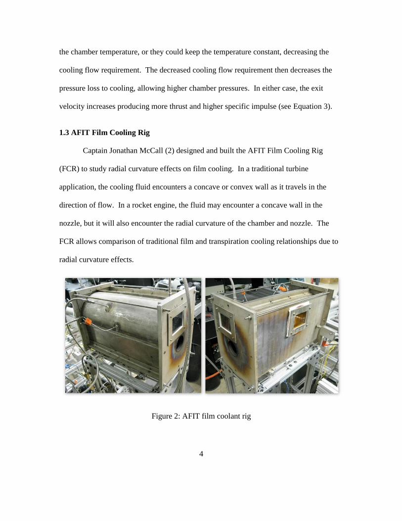
Captain Jonathan McCall (2) designed and built the AFIT Film Cooling Rig

(FCR) to study radial curvature effects on film cooling. In a traditional turbine

application, the cooling fluid encounters a concave or convex wall as it travels in the

direction of flow. In a rocket engine, the fluid may encounter a concave wall in the

nozzle, but it will also encounter the radial curvature of the chamber and nozzle. The

FCR allows comparison of traditional film and transpiration cooling relationships due to

radial curvature effects.

Figure 2: AFIT film coolant rig

5

Figure 2 shows the FCR after the modifications accomplished in this thesis. Test

sections with varying curvature, hole size/orientation, or a number of other variables are

easily tested due to the modular design of the FCR. Three view ports allow access for

non-intrusive combustion diagnostic techniques. Stainless steel construction allows high

temperatures and combustion environments. Finally, a water cooling system

accommodates the high-temperature combustion environment and allows heat flux

measurements.

1.4 Research Purpose

The purpose of this research is to modify the FCR and demonstrate its operation,

to include film cooling of a radially curved wall. While the initial FCR design called for

a combustion environment, previous research stopped well short of actual

implementation. The modification tasks include design and build of the burner, ignition

system, water-cooling system, and stainless steel test sections. In addition to the FCR

changes, modification to the water delivery system, the fuel delivery system and the

LabVIEW® computer program are also necessary.

Once modifications are complete, infrared thermography will capture the coolant

effects on the wall yielding cooling efficiency statistics. The modified FCR will also

allow laser diagnostic techniques to characterize the combustion environment and coolant

flow in the film-cooled region.

Chapter 2 will describe the fundamentals of rocket engine performance and

effusion cooling. It will also cover the research progress preceding this work. Chapter 3

details the experimental setup and modifications to the FCR while chapter 4 details the

6

experimental results. Finally, chapter 5 contains the conclusions, lessons learned, and

suggestions for future research.

7

II. Literature Review

2.1 Rocket Engines

For a rocket to launch a payload into space, it must convert the latent energy

stored inside its fuel into propulsive force (thrust). Chemical systems such as liquid,

solid, and hybrid-fueled rockets use the energy present in the chemical bonds of the

propellant to generate thrust. Alternatively, electrical propulsion systems use

electrothermal, electromagnetic, or electrostatic thrust generation techniques (3). Modern

space launch vehicles often use a combination of solid and liquid systems, while electric

propulsion is limited to space applications due to the lower thrust levels. Any numbers of

textbooks covering rocket propulsion document the benefits and drawbacks of solid

versus liquid systems as summarized in Table 1 (3)(4).

Table 1: Solid vs. liquid fuel advantages

Solid Liquid

High thrust High ISP

Simplicity Throttling

Storable Restartable

The mission designer must evaluate each mission to determine what combination of solid

and/or liquid fuel systems will meet their thrust and Isp requirement.

Both solid and liquid fueled rockets require cooling for both the combustion

chamber and nozzle regions due to the extremely high temperatures and pressures. The

8

main cooling options include regenerative, ablative, and film cooling (3). In addition, the

heat may simply radiate to the surrounding environment. The presence of liquid fuel and

oxidizers make regenerative and effusion cooling options for liquid systems; solids are

limited to ablative and radiation cooling. Most large launch vehicles employ regenerative

cooling where the liquid fuel flows through small tubing brazed to the nozzle. The liquid

carries away the heat, not only cooling the wall, but also adding energy to the fuel. The

drawback to this approach is that it complicates manufacture of the nozzle and significant

pressure is lost through the small coolant tubes (2). The pressure loss in turn drives the

pump size (mass) and available pressure to the combustion chamber.

2.2 Effusion Cooling Basics

Before addressing the literature on effusion cooling, it is useful to provide some

background on the technique itself and the various parameters that define it. In any

effusion cooling scheme, coolant flow is added to the main flow of the engine, not with

the direct intent of adding to the work done by the engine, but rather to cool various

components in the engine.

2.2.1 Effusion Cooling Flow

The main parameter in defining effusion cooling is the ratio of the coolant flow

flux to main flow flux, also known as the Blowing Ratio (F).

c cvF

u

(4)

where ρc is coolant density, νc is coolant velocity, ρ∞ is main flow density, ν∞ is main flow

velocity. In turbine engines, the blowing ratio is important because it represents air bled

9

off the compressor stage and diverted past the combustor. While the coolant flow adds

some energy to the cycle, there is a net loss when compared to the same inlet flow with

no diverted coolant (5). For rocket engine applications, the blowing ratio may be even

more important due to the need to carry the coolant onboard the vehicle itself, versus an

aircraft capturing the coolant from the surrounding environment.

Another useful effusion cooling parameter is the momentum ratio (I), the ratio of

the coolant flow to the main flow momentum:

2

2

c cvI

u

(5)

The momentum ratio is important in defining how the kinetic energy of the main flow

and the cooling flow interact. Physically this interaction is observed in how the coolant

jet turns when injected off-axis from the main flow. The momentum ratio also affects the

maximum coolant mass flux before the coolant stops coating the wall in a film-like

manner and starts jetting into the main flow (2).

The density ratio (DR) is simply the ratio of the cooling flow density to the main

flow:

cDR

(6)

Research has considered the effects of the density ratio on film cooling, but mostly on a

scale that applies to aircraft. In the typical rocket engine with cryogenic fuels injected

into a hot chamber, the density ratio can be orders of magnitude greater than aircraft

engine applications (2).

10

2.2.2 Transpiration Cooling Efficiency

Transpiration cooling is essentially just convective heat transfer from the main

flow to the cool wall combined with a mass transfer from the cool wall into the main

flow. The Stanton number (St) characterizes the convective heat transfer involved in

transpiration cooling. McCall(2) characterized the Stanton number as the heat transfer

perpendicular to a wall in a flow to the heat transfer parallel to the wall:

(7)

(7)

where St is the Stanton number, is heat flux into surface, cp,∞ is specific heat (at

constant pressure), and is main flow mass flux. Modifying Equation 7 is possible by

recognizing the temperature difference factor in the surface heat flux.

(8)

(8)

where h is the heat transfer coefficient. Typical transpiration cooling analysis ignores

radiation from the main flow to the wall because it is a small percentage of the total heat

transfer.

The cooling efficiency (ηt) of transpiration cooling is the ratio of cooled Stanton number

to uncooled Stanton number, or even more specifically, the ratio of the two heat transfer

coefficients:

0 0

t

St h

St h (9)

11

2.2.3 Film Cooling Efficiency

While the blowing ratio defines the flow of the coolant and main flow, it does not

give any insight into cooling performance. The film cooling efficiency, or adiabatic

effectiveness, quantifies the performance of film cooling. Adiabatic effectiveness is the

ratio of the temperature reduction of an adiabatic wall due to film cooling to the

temperature difference between the main flow and the coolant flow.

awf

c

T T

T T

(10)

where ηf is film cooling efficiency (adiabatic effectiveness), T∞ is main flow recovery

temperature, Taw is adiabatic wall temperature (cooled), and Tc is coolant temperature.

When the wall is the same temperature as the main flow, the efficiency is zero.

Conversely, the efficiency is one when the wall is the same temperature as the coolant

flow.

As coolant flows out of the coolant channels and onto the wall it will eventually

evaporate or mix into the main flow. Averaging the adiabatic effectiveness perpendicular

to the flow highlights this effect when plotted vs. streamwise distance from the coolant

hole. Equation 11 shows this spanwise adiabatic effectiveness.

2

12 1

1span f dx

(11)

12

The origin in this example is at the middle of the coolant hole; the x axis is in the radial

direction while the y axis is in the streamwise direction. ζ is often the lateral distance

between film cooling holes, although it is also useful to describe any region of interest1.

Finally, the entire cooling effect is describable using the area-averaged adiabatic

effectiveness:

2 2

1 12 1 2 1

1 1area f dxdy

(12)

In this last case, γ is often the spacing between film cooling holes (streamwise), although

other values may be appropriate in certain situations as with ζ.

2.3 History of Effusion Cooling Research for Rockets

With the availability of liquid fuel and oxidizer, effusion cooling is another option for

liquid fueled rockets. Much of the literature relevant to film cooling applications in

rocket engines is traceable to Duncan Rannie (6) at the Jet Propulsion Laboratory (JPL)

in the 1940‘s. Rannie was a student of von Karman at JPL and his work coincides with

some of the early American development of modern rocket applications taking place at

JPL in this era. A notable early application of film cooling for a rocket engine occurred

when Aerojet2 demonstrated chamber film cooling in 1967 with the ARES 100,000 Lbf

thrust chamber (7). Unlike the work of Rannie and other transpiration researchers using

porous materials, the ARES experiments used photo etched metal plates (platelets)

bonded together to provide the coolant to the transpiration cooled surface. The platelet

1 For example, in transpiration cooling the hole spacing is small and variable, so it may be necessary to

choose values of ζ and γ based on the hardware geometry or other parameters. 2 Aerojet itself started by von Karman and a number of his students from Cal Tech (and JPL)(34)

13

construction addresses one of the principal shortcomings in transpiration cooling for

rockets: the difficulty in manufacturing a porous material that effectively delivers coolant

in the presence of a pressure gradient (as found in the throat region). Despite this early

work on effusion cooling applications for rocket engines, modern rocket engines such as

the Space Shuttle Main Engines (SSME) utilize film cooling only for the injector faces

(8). Large rocket engines do not typically employ full coverage film cooling on the

combustion chamber or nozzle walls.

In the mid-1990‘s a number of AFIT students performed experimental and numerical

studies on transpiration cooling applications for rocket engines. Previous students used a

low speed shock tunnel to investigate transpiration-cooling effects on flat plates. Lenertz

(9) began a series of research using the same shock tunnel, but with a Mach 2.0 nozzle

cooled via transpiration cooling. Later, Landis (10) numerically demonstrated that the

Space Shuttle Main Engine (SSME) chamber walls would be 35% cooler using

transpiration cooling instead of regenerative cooling. While these students investigated

the nozzle cooling problem specific to rockets, they never addressed the curvature effects

of the nozzle when compared to a flat plate. More recently, McCall‘s research (2) is

notable for specifically addressing the radial curvature effects present in a rocket engine.

In a departure from the previous AFIT studies, McCall looked at film cooling effect in a

radial section, showing that increasing curvature generally increases cooling efficiency,

up to a point.

14

2.3.1 Early Transpiration Cooling Models

In 1947, researchers at JPL delivered a series of reports for a missile program

contracted to JPL by Air Material Command. Progress report 4-50, A Simplified Theory

of Porous Wall Cooling by W.D. (Duncan) Rannie (6) contained both analytical

predictions of transpiration cooling efficiency as well as experimental results to back up

those predictions. Rannie related the temperature change to the blowing ratio as shown

in Equation 13.

0.1 0.137 Re 37 Re Pr0.11 1.18Re 1 1

F Fc

w c

T TR e e

T T

(13)

where R is the Rannie temperature ratio, Tw is wall temperature, Re∞ is the main flow

Reynolds number, and Pr∞ is the main flow Prandtl number. Rannie‘s experiments

considered only air/air interactions, and as McCall (2) points out, do not factor in the

difference between the physical characteristics (such as density) of the main flow and the

coolant. In addition, the Rannie model overestimates actual cooling performance by

about 15% (11).

Spalding (12) later proposed a general solution to the mass transfer problem as:

(14)

where is coolant mass flux, g is the surface conductance, and B is the driving force.

Furthermore, the surface conductance is:

,p mix

hg

c (15)

where cp, mix is the specific heat of the mixture, and h is the heat transfer coefficient.

Spalding showed that the driving force for the transpiration cooling problem is:

15

,

,

p w

p c w c

c T TB

c T T

(16)

where Tw is surface wall temperature. Spalding neglected radiation and assumed the

specific heats were the same although they are shown here for completeness. The surface

heat transfer coefficient is found using Spalding‘s relationships, leading back to the

transpiration cooling efficiency (Equation 9).

Later developments by Simpson, Kays, and others (13) at Stanford bridge the gap

to more recent transpiration cooling research. Spalding (12) expressed the cooling

efficiency in terms of the blowing ratio as shown in Equations 17 and 18.

,0 0

ln 1f

f

C BSt

C St B

(17)

where Cf is the cooled skin friction coefficient, Cf,0 is the un-cooled skin friction

coefficient, and:

F

BSt

(18)

Simpson et al. (13) experimentally determined the Stanton number and skin friction

factor as a function of the blowing ratio (F) and the momentum Reynolds number (Reθ),

modifying Equation 17 as shown in Equation 19.

0.7

0.25ln 1

0.0130 Re2

fC BSt

B

(19)

At the time, a number of researchers published experimental transpiration cooling data

and Simpson sought to evaluate the other data and set conditions for qualification of the

test apparatus. The qualification included verifying the un-cooled friction factor (Cf),

16

Stanton number (St), mean velocity profile (U∞), and boundary layer thickness. The

qualification proved the accuracy of Simpson‘s test data, something he questioned when

evaluating the previous research.

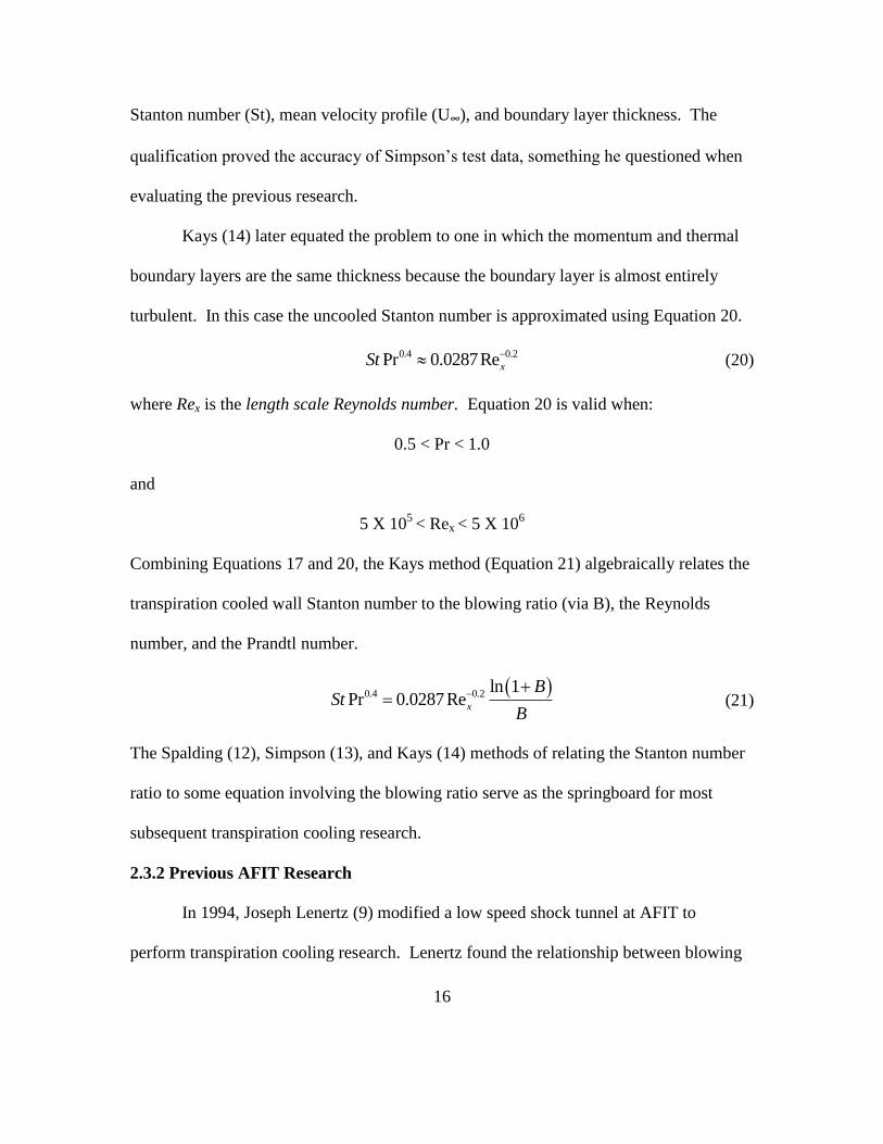
Kays (14) later equated the problem to one in which the momentum and thermal

boundary layers are the same thickness because the boundary layer is almost entirely

turbulent. In this case the uncooled Stanton number is approximated using Equation 20.

0.4 0.2Pr 0.0287RexSt (20)

where Rex is the length scale Reynolds number. Equation 20 is valid when:

0.5 < Pr < 1.0

and

5 X 105

< Rex < 5 X 106

Combining Equations 17 and 20, the Kays method (Equation 21) algebraically relates the

transpiration cooled wall Stanton number to the blowing ratio (via B), the Reynolds

number, and the Prandtl number.

0.4 0.2

ln 1Pr 0.0287Rex

BSt

B

(21)

The Spalding (12), Simpson (13), and Kays (14) methods of relating the Stanton number

ratio to some equation involving the blowing ratio serve as the springboard for most

subsequent transpiration cooling research.

2.3.2 Previous AFIT Research

In 1994, Joseph Lenertz (9) modified a low speed shock tunnel at AFIT to

perform transpiration cooling research. Lenertz found the relationship between blowing

17

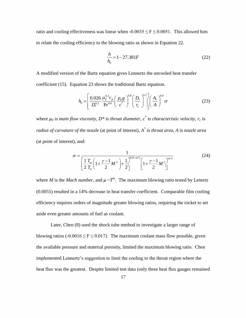
ratio and cooling effectiveness was linear when -0.0035 ≤ F ≤ 0.0051. This allowed him

to relate the cooling efficiency to the blowing ratio as shown in Equation 22.

0

1 27.381h

Fh

(22)

A modified version of the Bartz equation gives Lennertz the uncooled heat transfer

coefficient (15). Equation 23 shows the traditional Bartz equation.

0.10.8 0.90.2

0 0 * *0 0.2 0.6 *

*

0.026

Pr

p

c

c p g D Ah

D c r A

(23)

where μ0 is main flow viscosity, D* is throat diameter, c* is characteristic velocity, rc is

radius of curvature of the nozzle (at point of interest), A* is throat area, A is nozzle area

(at point of interest), and:

0.8 /5 /5

2 2

0

1

1 1 1 11 1

2 2 2 2

m m

wTM M

T

(24)

where M is the Mach number, and μ ~Tm. The maximum blowing ratio tested by Lenertz

(0.0055) resulted in a 14% decrease in heat transfer coefficient. Comparable film cooling

efficiency requires orders of magnitude greater blowing ratios, requiring the rocket to set

aside even greater amounts of fuel as coolant.

Later, Chen (8) used the shock tube method to investigate a larger range of

blowing ratios (-0.0016 ≤ F ≤ 0.017). The maximum coolant mass flow possible, given

the available pressure and material porosity, limited the maximum blowing ratio. Chen

implemented Lennertz‘s suggestion to limit the cooling to the throat region where the

heat flux was the greatest. Despite limited test data (only three heat flux gauges remained

18

operational), Chen proposed the following modification to the Lenertz efficiency

calculation:

0

1 38h

Fh

(25)

Although never stated explicitly, Chen asserts that the cooling efficiency relationship is

linear through his test range. Casual observation of Chen‘s cooling efficiency vs.

blowing ratio figure raises the question of whether a higher order curve fit would be more

appropriate.

Figure 3: Chen‘s experimental transpiration cooling efficiency (8)

Unfortunately, Chen does not provide actual cooling efficiency and blowing ratio data.

Chen also used a shadowgraph system to verify that the boundary layer did not grow

significantly at this blowing ratio, a concern raised by Keener (16). Keener previously

showed that the exit Mach number (and velocity) decreased with increased blowing

ratios, decreasing thrust as shown in Equation 1.

19

Following Chen, Landis (10) developed a computer model for transpiration

cooling of the Space Shuttle Main Engines. The maximum blowing ratio was limited to

0.010 to stay consistent with Chen. Landis demonstrated that the SSME could be

transpiration cooled using a blowing ratio of only 0.004 and that a hot side temperature

decrease of 35% is possible for a blowing ratio of 0.010. The computer model also

showed the heat flux increased with porosity, although he contributed the increase in heat

flux to the decrease in surface area of the larger spheres constituting the higher porosity

test cases models. One important result of Landis‘ work was his finding that the

transpiration cooled wall thermal gradient was 72 times the regeneratively cooled wall.

The temperature gradient may be a major factor in material selection for transpiration

cooled walls.

2.3.3 Current AFIT Research

Immediately preceding this work, McCall (2) designed and built the FCR. More energy

is devoted to reviewing McCall‘s research as this effort springs directly from his work.

While most of the research cited by McCall concerns transpiration cooling, he starts by

using a computational fluid dynamics (CFD) simulation to modify the Rannie

transpiration model (Equation 13) for full coverage film cooling (FCFC). First,

combining Equations 10 and 13 yields:

1

1fR

(26)

McCall curve-fit the plot of area

f

(Equations 12 and 26) vs. the film cooling area ratio (S)

as shown in Equation 27:

20

224.2792 4.4087 0.0755area

t

S S

(27)

The film cooling simulation results approached the transpiration cooling calculations as

the spacing between the holes decreased. For the hole spacing cited by McCall as most

likely for rocket engine applications, the film cooling effectiveness was only 10-17% of

the transpiration cooling efficiency based on the Rannie model. Beyond this point,

McCall‘s research only addresses film cooling and not transpiration cooling.

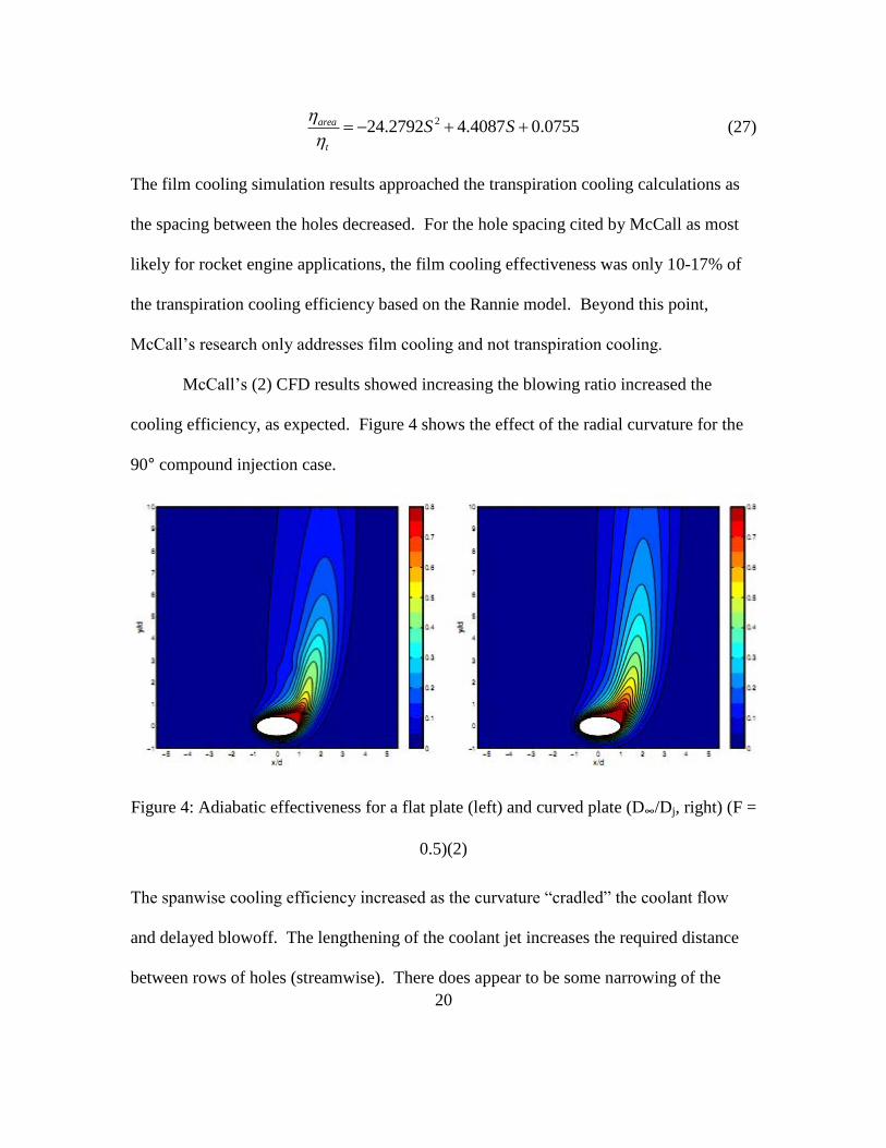
McCall‘s (2) CFD results showed increasing the blowing ratio increased the

cooling efficiency, as expected. Figure 4 shows the effect of the radial curvature for the

90° compound injection case.

Figure 4: Adiabatic effectiveness for a flat plate (left) and curved plate (D∞/Dj, right) (F =

0.5)(2)

The spanwise cooling efficiency increased as the curvature ―cradled‖ the coolant flow

and delayed blowoff. The lengthening of the coolant jet increases the required distance

between rows of holes (streamwise). There does appear to be some narrowing of the

21

coolant flow in the radial (x) direction although McCall does not provide a metric to

evaluate it. Presumably, less coolant in the radial direction leads to a decrease in the

coolant hole pitch, or radial spacing. A second expected result was that the increase in

spanwise efficiency was more pronounced at 90⁰ than at 45⁰ or 0⁰.

McCall (2) designed the FCR to accommodate data collection from a variety of

techniques. Some of the possible techniques include infrared thermography, planar laser

induced florescence (PLIF), particle image velocimetry (PIV), calorimetry (leading to

average heat flux), and emissions testing. Despite the choice of diagnostics, the scope of

McCall‘s research was limited to infrared measurement of air/air3 film cooling due to the

number of variables he tested. The test variables include compound injection angle (α =

0º and 90º), density ratio (1.17, 1.76), diameter of curvature to hole diameter ratio (D∞/Dj

= 16.0, 32.2, 48.5, 64.4, 97.0), and presence of a stream-wise pressure gradient

(with/without—not characterized). The blowing ratio varied between 0.50 and 1.50 for

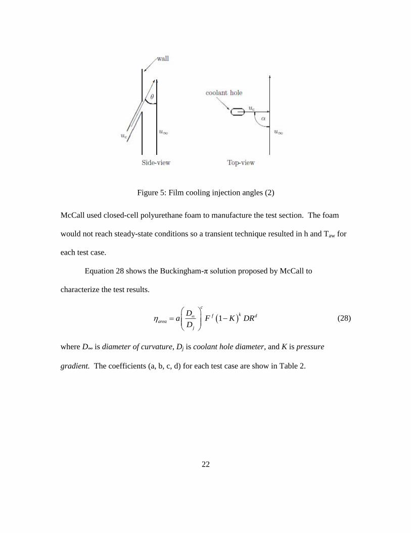
all cases and the injection angle into the flow (θ) was 30°. Figure 5 shows the two film

cooling injection angles, α and θ.

3 air/air refers to the main and coolant flows respectively

22

Figure 5: Film cooling injection angles (2)

McCall used closed-cell polyurethane foam to manufacture the test section. The foam

would not reach steady-state conditions so a transient technique resulted in h and Taw for

each test case.

Equation 28 shows the Buckingham-π solution proposed by McCall to

characterize the test results.

1

c

kf d

area

j

Da F K DR

D

(28)

where D∞ is diameter of curvature, Dj is coolant hole diameter, and K is pressure

gradient. The coefficients (a, b, c, d) for each test case are show in Table 2.

23

Table 2: McCall‘s Experimental Coefficients (2)

McCall‘s (2) results are specific to his experiment because the limits of integration for

ηarea, area are not linked to a definition of coolant row spacing and/or hole pitch. Future

experimentation with multiple holes may remedy this issue. Despite this limitation in

Equation 28 and its coefficients, McCall‘s research proved that increasing curvature

increases cooling efficiency when the coolant encounters a concave surface (due to

compound injection). The cooling effectiveness decreased without compound injection.

In addition to the curvature results, McCall (2) proved the streamwise pressure

gradient improved cooling efficiency by delaying blow-off, as did an increasing density

ratio (ρc/ρ∞).

McCall (2) provided multiple recommendations serving as the starting point for

this research. Two of McCall‘s suggestions address refinements to the simulation and

modeling effort. He also recommends studying variations in Reynolds number and

turbulence levels in the context of radial curvature, as well as utilizing combustion

diagnostics (such as PLIF and PIV) with fuel-based coolant in a combustion environment

to calculate performance effects (on thrust and Isp).

24

2.4 AFIT Test Capability

The AFIT COAL Lab is rapidly expanding its capability to perform modern laser

diagnostic techniques for combustion analysis. Recent years have seen a series of

students focusing their research on Planar Laser Induced Florescence (PLIF) for the Ultra

Compact Combustor (UCC). In addition, one student recently detailed Particle Image

Velocimetry (PIV) for the combustion environment of the UCC. Finally, portable

infrared cameras are available for temperature measurement. McCall (2) used the

infrared camera for his research while Bohnert (17) investigated a Hall thruster inside a

vacuum chamber with the same camera.

2.4.1 COAL Lab Setup and PLIF for the UCC

Anderson (18) designed and built the COAL lab for his thesis work in 2006-2007.

Lab setup consumed most of Anderson‘s time, although he discusses a number of

intended diagnostic techniques to include: Coherent Anti-Stokes Raman Scattering

(CARS), Laser Induced Incandescence (LII), PLIF, and PIV. Koether (19) and Hankins

(20) went on to further refine the COAL lab and actually performed PLIF with a Hencken

burner (a burner capable of producing a laminar premixed flame). Lakusta (21) was the

first student to utilize PLIF in the UCC; he was not able to get temperature or species

concentrations from his data, but did identify flame locations inside the UCC cavity-vane

area. Lakusta recommended, and Drenth (22) implemented two-color PLIF to obtain

temperature data inside the UCC.

25

Figure 6: OH concentrations inside the UCC (22)

Drenth refined and documented the methodology to obtain OH concentration using PLIF.

Figure 6 shows a false-color image of the OH intensity inside the UCC. Drenth‘s work is

the best source for current COAL lab documentation and procedures. Even though

Drenth used the UCC for his research, many of the gas delivery system and laser systems

that he describes are also used by the FCR. Drenth also described the experimental

technique to acquire time and spatially averaged temperature data. Signal-to-noise

limitations forced Drenth to average temperature data, although he did describe various

upgrades to both the laboratory and the UCC to increase the PLIF signal.

2.4.2 PIV in the UCC

Thomas (23) departed from previous UCC research to perform PIV inside the

UCC. Thomas used PIV to obtain 2-D data for velocity, turbulence, and vorticity in the

combustion zone. Silicon carbide particles served as the seed material for the PIV due to

their high melting point. Figure 7 shows PIV data from the UCC.

26

Figure 7: PIV data in the UCC (23)

Thomas used a different laser, camera, and computer equipment then Drenth (22),

although many of their optics were compatible. The PIV setup rests on a wheeled cart

and numerous labs at AFIT share the equipment.

2.4.3 Infrared Thermography

The infrared energy emitted by an object is a function of that objects temperature.

Infrared imaging captures the intensity of the infrared radiation onto a 2-D focal plane

where the voltage at each pixel corresponds to the energy absorbed by that pixel. The

voltage translates into a temperature, based on the camera and user defined settings.

Bohnert (17) describes the science behind infrared thermography in his thesis on Hall

thrusters. Figure 8 shows the possible sources of energy measured by the infrared

camera.

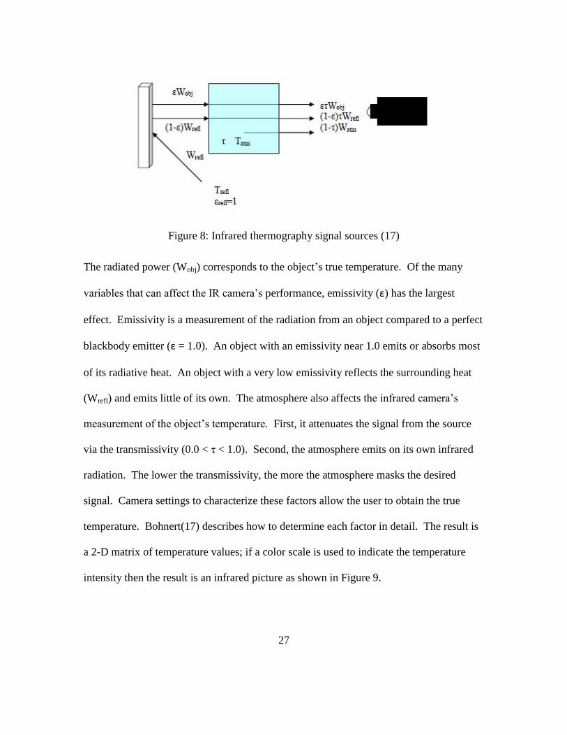
27

Figure 8: Infrared thermography signal sources (17)

The radiated power (Wobj) corresponds to the object‘s true temperature. Of the many

variables that can affect the IR camera‘s performance, emissivity (ε) has the largest

effect. Emissivity is a measurement of the radiation from an object compared to a perfect

blackbody emitter (ε = 1.0). An object with an emissivity near 1.0 emits or absorbs most

of its radiative heat. An object with a very low emissivity reflects the surrounding heat

(Wrefl) and emits little of its own. The atmosphere also affects the infrared camera‘s

measurement of the object‘s temperature. First, it attenuates the signal from the source

via the transmissivity (0.0 < τ < 1.0). Second, the atmosphere emits on its own infrared

radiation. The lower the transmissivity, the more the atmosphere masks the desired

signal. Camera settings to characterize these factors allow the user to obtain the true

temperature. Bohnert(17) describes how to determine each factor in detail. The result is

a 2-D matrix of temperature values; if a color scale is used to indicate the temperature

intensity then the result is an infrared picture as shown in Figure 9.

28

Figure 9: Infrared picture of a Hall thruster (17)

The accuracy of the temperature measurement is tied to the accuracy in defining

the camera settings. Infrared thermography is especially useful for this research because

the cooling efficiency is a factor of temperature differences and not absolute

temperatures, minimizing bias error due to incorrect camera settings.

29

III. Methodology

3.1 Research Objectives

The FCR was initially intended as a combustion experiment, although McCall

ultimately decided to perform his experimentation using only hot air. The introduction of

a combustion environment to the FCR required a number of modifications to the rig

itself, as well as the laboratory support systems. The research objectives for this thesis

included:

Build curved test section articles. Previously the FCR experiment used foam

curved sections to test air/air film cooling. The combustion upgrade required

stainless steel test sections. The material change significantly complicated

manufacture and instrumentation of the test section.

Design/test burner system. The burner system provides the combustion source for

the FCR. The burner design must provide proper mass flow rates without

instability or risk of flameout.

Design/test heat flux measurement system. While McCall designed the FCR with

a water-cooling/heat flux measurement system in mind, it was never

implemented. The system included changes to the FCR, the laboratory, and

instrumentation for the heat flux measurements.

Develop/test appropriate operating regime. Once the combustion modifications

were completed, the test conditions for the main flow, coolant flow, and water-

cooling flow were determined. In addition, the LabVIEW® control software

30

required modification to increase its usefulness and applicability to the FCR.

Finally, infrared thermography and calorimetry results attempted to validate the

hardware design.

3.2 Laboratory Setup

The AFIT COAL (Combustion Optimization and Analysis Laboratory) laboratory

facilitates research on the Ultra Compact Combustor (UCC), a radial combustion

chamber design intended to reduce the length (and weight) of the combustion chamber in

gas turbine engines (as commonly seen in aircraft.) The radial burning concept in the

UCC also has the potential to increase the efficiency of the engine (22). A series of AFIT

Masters students have designed, built, upgraded, and redesigned the COAL lab. McCall

(2) first used the lab for non-UCC related research with the FCR. Chapter 2 described

some of the UCC research using PLIF and PIV while others have accomplished Laser

Induced Incandescence (LII) and Tunable Diode Laser Absorption Spectroscopy

(TDLAS). Both portable and laboratory grade emissions analysis equipment are also

available.

The COAL lab consists of three major systems and a variety of other equipment

for use in various experiments. The three major systems are the fuel/air delivery system,

the exhaust system, and the control system. Most experimentation in this laboratory uses

all three systems. Other equipment, such as the various lasers, is used selectively for

individual experiments. The three major systems are discussed next, while the equipment

used for testing will be discussed in the related sections.

31

3.2.1 Fuel/Air Delivery Systems

The tank farm is an area outside building 640 at AFIT that houses the propane for

the FCR burner, the air, and ethylene used in the igniter, as well as a variety of other

gases used in the AFIT laboratories. The gaseous ethylene and zero (pure) air are stored

in ―K‖ type bottles, while liquid propane is stored in three larger 150-gallon tanks.

Figure 10 shows both the smaller K bottles and the larger propane tanks. Figure 11

shows the gas flow path for each gas used by the FCR. Complete procedures for

operation of the gas system are given by Drenth (22).

Figure 10: K bottles (left), propane tanks (right), and propane vaporization system (upper

right) inside the tank farm

32

Figure 11: FCR gas flow diagram

Most of the gasses from the tank farm run through copper tubing to a bank of

valves on the north wall of the COAL lab. The ethylene and air lines for the FCR igniter

are included in these valves. From there, the gas connects to the test stand with

polyethylene tubing routed over the superstructure. The test stand routes each gas

through a solenoid valve, filter, and mass flow controller (MFC) as shown in Figure 12.

Figure 12: Test stand setup

Mass Flow

Controllers

Mass Flow

Controllers

Filters

Solenoid

Valves

33

The operator controls the solenoid valves through the LabVIEW® VI (described in

section 3.2.3); the MFCs are controlled with one of the two MKS type 247 digital readout

panels shown in Figure 13.

Figure 13: Control panels for MFCs

The setting for each channel is a function of the gas and the MFC for that channel. The

procedure to set the MFC is given in Appendix B. The FCR used four channels for the

igniter fuel, igniter air, propane coolant, and propane main flow fuel. Table 3

summarizes the fuel system setup for the FCR.

Table 3: Gas system summary

Gas storage Flow Control Operator Control

Igniter fuel ethylene (C2H4) K bottle 20 SLPM (N2) MFC MKS control panel

Igniter air zero air K bottle 50 SLPM (air) MFC MKS control panel

Film coolant propane (C3H8) 150 gallon tanks 100 sccm (Xe) MFC MKS control panel

Main flow fuel propane (C3H8) 150 gallon tanks 50 SLPM (N2) MFC MKS control panel

Main flow air laboratory

compressed air

6000 gallon tank

(shared)

flow meter/pneumatic

valve

LabVIEW®-

secondary air

34

The liquid propane is vaporized with a heat vaporization system in the tank farm

(visible in Figure 10). The system was installed for use with a Sulzer Metco High

Velocity Oxy-Fuel (HVOF) Diamond Jet® spray gun. The manufacturer markets the

Diamond Jet® for high temperature surface coating applications. AFIT uses the HVOF

system for high temperature material testing inside the COAL laboratory. The FCR

originally used a smaller traditional gaseous propane tank (100 lb), but eventually

switched to the larger liquid tanks due to large amount of propane used during testing.

The propane enters the COAL lab in a separate location from the remainder of the gasses

from the tank farm. Figure 14 shows the HVOF panel.

Figure 14: HVOF control panel

The propane enters at the bottom center of the figure, runs through a ball valve, a

pneumatic valve, and then a needle valve with a rotary control knob. A rotameter shows

the flow rate and pressure gauges display the upstream and downstream pressure. A lab

35

tech forced the pneumatic valve to the open position by disconnecting the air-out line and

switching the air-in line to the air-out connector. Forcing the pneumatic valve to the open

position simplifies startup procedures by eliminating the need to start the computer and

LabVIEW® VI controlling the HVOF setup. Even after removing the pneumatic valve

there are still the two valves on the control panel to regulate propane flow, in addition to

eight valves in the tank farm, and a solenoid valve and mass flow controller at the test

stand. The HVOF panel propane outlet was connected to the test stand in the same

manner as the other gasses, although the flow was split to both the main flow and coolant

mass flow controllers.

The airflow setup is completely different than the other gasses for the COAL lab.

The main airflow comes from a 6000 gallon pressurized tank outside the lab. Two

Ingersoll-Rand compressors in an adjacent building supply compressed air to the tank,

although one broke down during testing. Figure 15 shows the air supply tanks.

Figure 15: Air supply tanks

36

The AFIT supersonic wind tunnel shares the tank, and it has the capability to empty the

entire tank in seconds. COAL lab operations must be coordinated with the wind tunnel

operations to ensure the air supply is not lost during testing.

After entering the lab, the air splits into two lines: the main and secondary line.

The FCR only uses the secondary air line. A Fox FT-2 mass flow meter measures the

mass flow rate, while a pneumatic valve controls the flow based on operator input to the

LabVIEW® VI. Figure 16 shows the flow meter and valve for the air supply.

Figure 16: Flow meter and valve for air supply

Further information on the air supply hardware, installation, and design choice is

available in the thesis by Dittman (24) and Anderson (18).

3.2.2 Exhaust System

Stainless and galvanized steel ductwork exhausts the hot gas from the FCR to

outside the building. Lakusta (21) installed dual fans to provide redundancy in case of

failure. Together, the fans move approximately 108,000 SLPM of air. The current

configuration allows vertical installation of the FCR (as with McCall (2)) or horizontal

37

installation (current setup). Doors over the room exhaust vents isolate the lab from the

other parts of the building during testing.

3.2.3 Control System

Figure 17: COAL lab master control station

The COAL lab Master Control Station (MCS, Figure 17) allows complete control

of most COAL lab functions from one central station. In the top-center of Figure 17 are

the two MKS Type 247 MFC control panels. To the right are emissions testing

equipment. Dittman (24) first discussed the California Analytical Instruments (CAI) gas

test bench, although Anderson (18) goes into more detail. COAL lab testing has not

employed the CAI test bench to date. AFIT installed the Agilent 5975 series Gas

Chromatograph (GC) and Mass Selective Detector (MSD) during this research. Future

research may utilize the GC/MSD to investigate combustion efficiencies in the UCC. In

the left of Figure 17 are a 52‘‘ monitor and computer capable of displaying information

38

from any of the other eight computers in the COAL lab. The FCR testing used this

monitor to display the thermal camera control software and a live video feed. Not shown

in the picture are the data acquisition system and myriad of wiring necessary to connect

the various sensors to the MCS.

The heart of the MCS is the central computer running LabVIEW® software.

Dittman (24) pioneered LabVIEW® in the lab, while many of the subsequent students

added functionality. Figure 18 shows the LabVIEW® interface used by McCall (2) and

Drenth (22).

Figure 18: Original COAL lab LabVIEW® VI

39

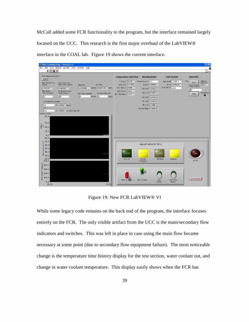
McCall added some FCR functionality to the program, but the interface remained largely

focused on the UCC. This research is the first major overhaul of the LabVIEW®

interface in the COAL lab. Figure 19 shows the current interface.

Figure 19: New FCR LabVIEW® VI

While some legacy code remains on the back end of the program, the interface focuses

entirely on the FCR. The only visible artifact from the UCC is the main/secondary flow

indicators and switches. This was left in place in case using the main flow became

necessary at some point (due to secondary flow equipment failure). The most noticeable

change is the temperature time history display for the test section, water coolant out, and

change in water coolant temperature. This display easily shows when the FCR has

40

reached steady-state conditions. The water outlet temperature allows the operator to

monitor the water temperature to avoid boiling inside the test section. There is no change

in how the various valves and airflow settings work, but the VI now performs many of

the calculations that were previously performed in others programs (MATLAB®,

Excel®) and kept in reference tables. The program determines the required air flow rate

when operator inputs the fuel flow rate from the MKS control panel, the desired

equivalence ratio. The operator is still required to manually input the air flow rate into

the secondary flow setting. In addition, the program displays the propane coolant flow

rate for each of the test blowing ratios. Appendix B provides more detail on operation of

the LabVIEW® program during testing.

3.3 Film Cooling Rig Modification

3.3.1 Test Section

This research updated the stainless steel test section design proposed by McCall

(2) (but not built). Once a viable design solution was reached, test sections were built

with curved section radii of 4‘‘ and 6‘‘, with compound injection angles of 0°, 45°, and

90° (6 total).

The curved wall of test sections match 4‘‘ and 6‘‘ schedule 40 pipe (102 mm and

154 mm inner radius). 316 Stainless steel pipe was chosen for the new test sections for

its high temperature, corrosion resistant properties, as well as to match the rest of the

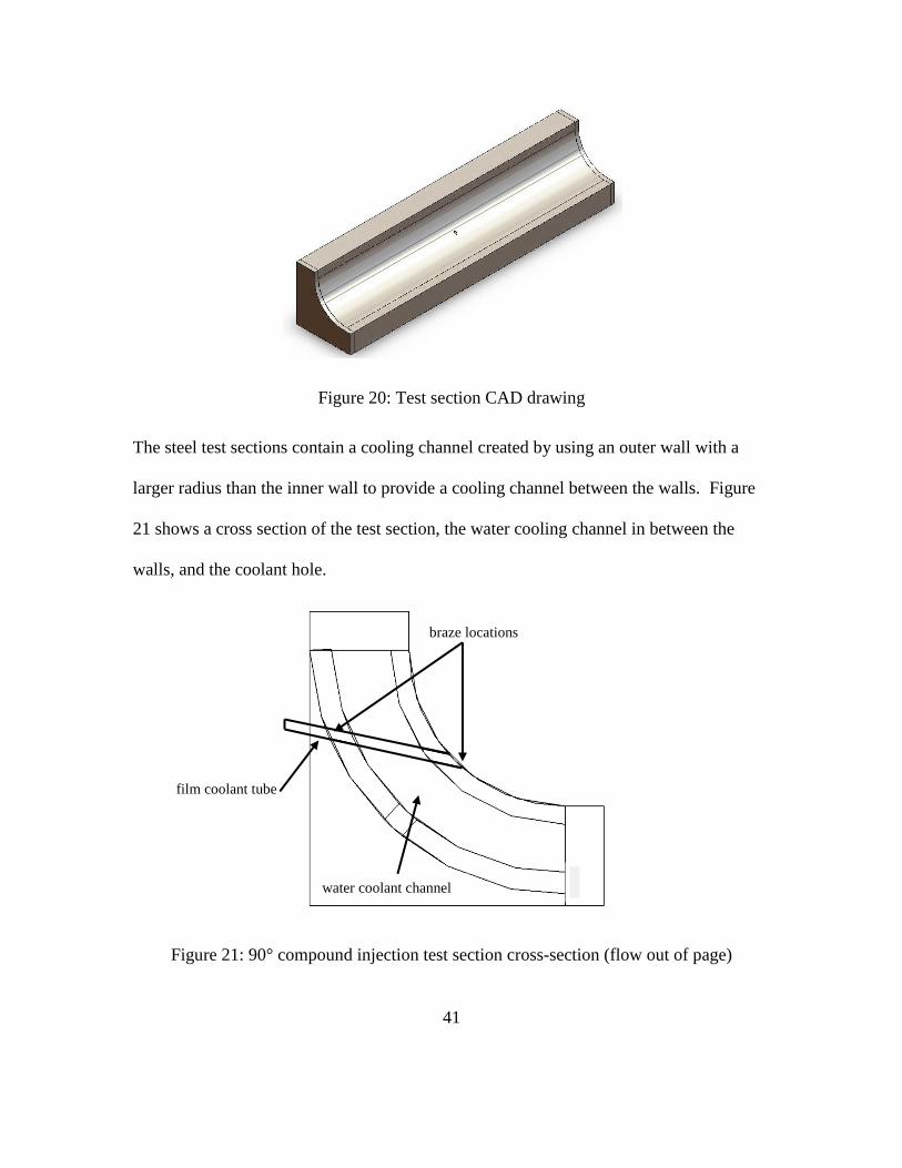
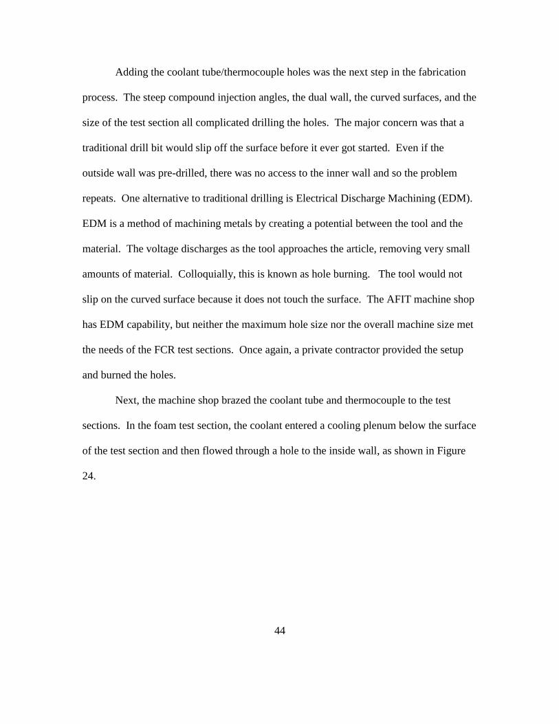
FCR. Figure 20 shows a CAD drawing of the stainless steel test section.

41

Figure 20: Test section CAD drawing

The steel test sections contain a cooling channel created by using an outer wall with a

larger radius than the inner wall to provide a cooling channel between the walls. Figure

21 shows a cross section of the test section, the water cooling channel in between the

walls, and the coolant hole.

Figure 21: 90° compound injection test section cross-section (flow out of page)

braze locations

water coolant channel

film coolant tube

42

There are three main features of the stainless steel test sections different from the foam

articles. First, the steel sections contain the cooling channel necessary to perform the

heat transfer analysis. Second, the cooling flow enters the FCR via a steel tube brazed in

place. Finally, the thermocouples were brazed through the walls of the test section.

The AFIT machine shop teamed with a local welding company to produce the

stainless steel test sections. First the machine shop cut necessary material to produce four

6‘‘ and four 4‘‘ inner radius test sections. Figure 22 shows the various parts that make up

one test section.

Figure 22: Exploded view of a test section

43

AFIT contracted the welding company because the test sections were beyond the

capability of the AFIT machine shop. The cost of the welding was significant though

necessary due to the overall complexity. After the test sections returned from welding,

the machine shop fit them to the FCR, drilled the necessary holes for attachment and the

coolant tube/thermocouple, and milled the curved section to a constant radius. A

computer controlled 3D end mill produced a precise 4‘‘ or 6‘‘ radius, correcting either

production flaws or warping due to the welding. The machinist avoided the ends of the

section, preventing compromise of the weld in those areas. The lip created by this

process is shown in Figure 23.

Figure 23: Machined lip on test section

The amount of material removed varied from section to section, even within a single

section. The most severe cases removed as much as 0.14‘‘, over half the thickness of the

material.

44

Adding the coolant tube/thermocouple holes was the next step in the fabrication

process. The steep compound injection angles, the dual wall, the curved surfaces, and the

size of the test section all complicated drilling the holes. The major concern was that a

traditional drill bit would slip off the surface before it ever got started. Even if the

outside wall was pre-drilled, there was no access to the inner wall and so the problem

repeats. One alternative to traditional drilling is Electrical Discharge Machining (EDM).

EDM is a method of machining metals by creating a potential between the tool and the

material. The voltage discharges as the tool approaches the article, removing very small

amounts of material. Colloquially, this is known as hole burning. The tool would not

slip on the curved surface because it does not touch the surface. The AFIT machine shop

has EDM capability, but neither the maximum hole size nor the overall machine size met

the needs of the FCR test sections. Once again, a private contractor provided the setup

and burned the holes.

Next, the machine shop brazed the coolant tube and thermocouple to the test

sections. In the foam test section, the coolant entered a cooling plenum below the surface

of the test section and then flowed through a hole to the inside wall, as shown in Figure

24.

45

Figure 24: McCall's cooling plenum (2)

The cooling channel of the stainless steel test section prevented a similar implementation

so the updated design included a 1/8‘‘ 316 stainless steel tube brazed into place. Brazing

offered the best combination of high temperature resistance with minimal effects on the

surrounding material. Figure 21 shows both braze locations for the coolant tube. The

thermocouples were also brazed into the test section, although they are not shown in the

figure.

The FCR was initially tested using JB-WELD® high temperature epoxy to secure

a 1/8‘‘ thermocouple in place (to test applicability in securing both the coolant tube and

thermocouple). Numerous issues presented themselves. First, it was very difficult to

produce a watertight seal with the JB-WELD®. Water leaked from the cooling channel

into the test section at even the lowest water flow rates. Next, it was very difficult to

apply a small amount of JB-WELD® and still produce a good seal. On the outside of the

test section sealing is not an issue, but on the inside the epoxy lump would unacceptably

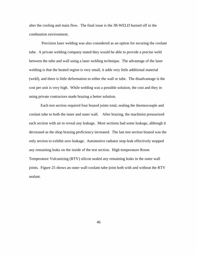
46

alter the cooling and main flow. The final issue is the JB-WELD burned off in the

combustion environment.

Precision laser welding was also considered as an option for securing the coolant

tube. A private welding company stated they would be able to provide a precise weld

between the tube and wall using a laser welding technique. The advantage of the laser

welding is that the heated region is very small, it adds very little additional material

(weld), and there is little deformation to either the wall or tube. The disadvantage is the

cost per unit is very high. While welding was a possible solution, the cost and they in

using private contractors made brazing a better solution.

Each test section required four brazed joints total, sealing the thermocouple and

coolant tube to both the inner and outer wall. After brazing, the machinist pressurized

each section with air to reveal any leakage. Most sections had some leakage, although it

decreased as the shop brazing proficiency increased. The last test section brazed was the

only section to exhibit zero leakage. Automotive radiator stop-leak effectively stopped

any remaining leaks on the inside of the test section. High temperature Room

Temperature Vulcanizing (RTV) silicon sealed any remaining leaks in the outer wall

joints. Figure 25 shows an outer wall-coolant tube-joint both with and without the RTV

sealant.

47

Figure 25: Coolant tube outer seal, braze on left, RTV on right

With the coolant tube and thermocouple attached, the test sections were nearly

complete. Final preparations for testing included attaching the tube fitting for both the

water and film coolant and painting the inner surface. The paint is further described in

the infrared testing section

3.3.2 Burner Design

Designing the burner proved one of the larger challenges in modifying the FCR.

Consideration was given to the existing design, desired flame type/shape, and desired

fuel/oxidizer flow rate. Ultimately, the total flow rate of air and fuel through the burner

was the driving factor because it directly ties this research to McCall‘s (2) work (via the

blowing ratio). In addition, the hardware associated with controlling the flow (mass flow

controller) is the most expensive and requires substantial lead-time.

The first step in designing the burner was selecting the fuel and oxidizer. Air was

the only choice for the oxidizer because the lab did not have enough oxygen available to

run the FCR, nor the correct size MFC to control it. In addition, at the beginning of

48

testing the lab did not have an available channel on the MFC to control another gas. The

secondary air supply did not rely on the MFC control panel, and the supply was plentiful.

Gaseous fuel was chosen to simplify the burner design and operation. The long-term

goal for the FCR is liquid-fuel combustion, similar actual rocket applications. The

COAL lab has a variety of fuel available (H2, C2H4, C3H8), but only the propane

(C3H8) was available in sufficient quantities to last the entire test program. Propane is

also a good choice because it is a very low producer of soot (25). Soot may fog the

windows and alter the laser and IR data. Adequately cleaning the soot from the FCR

windows may be a laborious process. Finally, a wealth of literature is readily available

on propane combustion.

To find the required propane and air mass flow rates, the combustion process for

propane with air was studied. Equation 29 shows the stoichiometric relationship for

propane-air combustion.

3 8 2 2 2 2 25( 3.76 ) 3 4 18.8C H O N CO H O N (29)

Equation 30 likewise gives the stoichiometric air-fuel ratio for hydrocarbon/air

combustion.

4.76

/1

fuel

stair

MWaA F

MW (30)

where a is number of moles of oxidizer (5), MWfuel is the fuel molecular weight (44.1

g/mol), and MWair is the air molecular weight (8.97 g/mol). The stoichiometric air-fuel

ratio is then 15.64, meaning it takes 15.64 grams of air to combust one gram of propane.

49

Actual testing may require either lean or rich mixtures, so the range of equivalence ratios

(φ) is needed to solve for the actual air-to-fuel ratio. The equivalence ratio is:

/

/

stA F

A F (31)

The lean flammability limit for propane is φ = 0.51, so a minimum test value of φ = 0.75

allows some margin. Similarly, the upper test limit was set at φ = 2.0, based on the rich

flammability limit of φ = 2.83 (25 p. 287). Using Equation 31, the range of air-to-fuel

ratio was, 7.82< (A/F) < 20.85. Equation 32 shows (A/F) is the ratio of the air and fuel

mass flow rates.

( / ) air

fuel

mA F

m (32)

Setting the fuel mass flow rate to the maximum possible rate for propane (based on the

available MFC), yields the air mass flow rate range. For the desired equivalence ratios

and the maximum propane mass flow rate (19 SLPM), the airflow rate was between

226.1 SLPM and 602.9 SLPM.

The first burner design was based on the inlet wall section already built but never

used in the previous research. The original (unused) inlet wall had a ¼‘‘ hole for the fuel

and oxidizer to enter the FCR. In an attempt to decrease the incoming turbulence,

McCall (2) instead built a three foot long aluminum tunnel to match the cross sectional

size of the FCR. Heated air entered at the bottom of the tunnel and flowed into the FCR.

For the combustion upgrade, the machine shop enlarged the hole to 3/8‘‘ (the maximum

possible given the existing inlet plate). The first burner design is shown in Figure 26.

50

Figure 26: Original burner design

It featured a co-axial propane-air flow through a 3/8‘‘ stainless steel ―T‖ fitting. The fuel

enters through 1/8‘‘ stainless tubing running through the middle of the fitting, while the

air comes in the side of the fitting and flows around the fuel tubing. Many production

rocket injectors use a similar co-axial design (26). Testing outside of the FCR showed

this size burner would never meet the mass flow requirements. In fact, only 16% (3.1

SLPM) of the required fuel flow and no air flow was ever possible before the flame blew

out. The fuel only flame is shown in Figure 27, lifted significantly off the burner and

about to blow out.

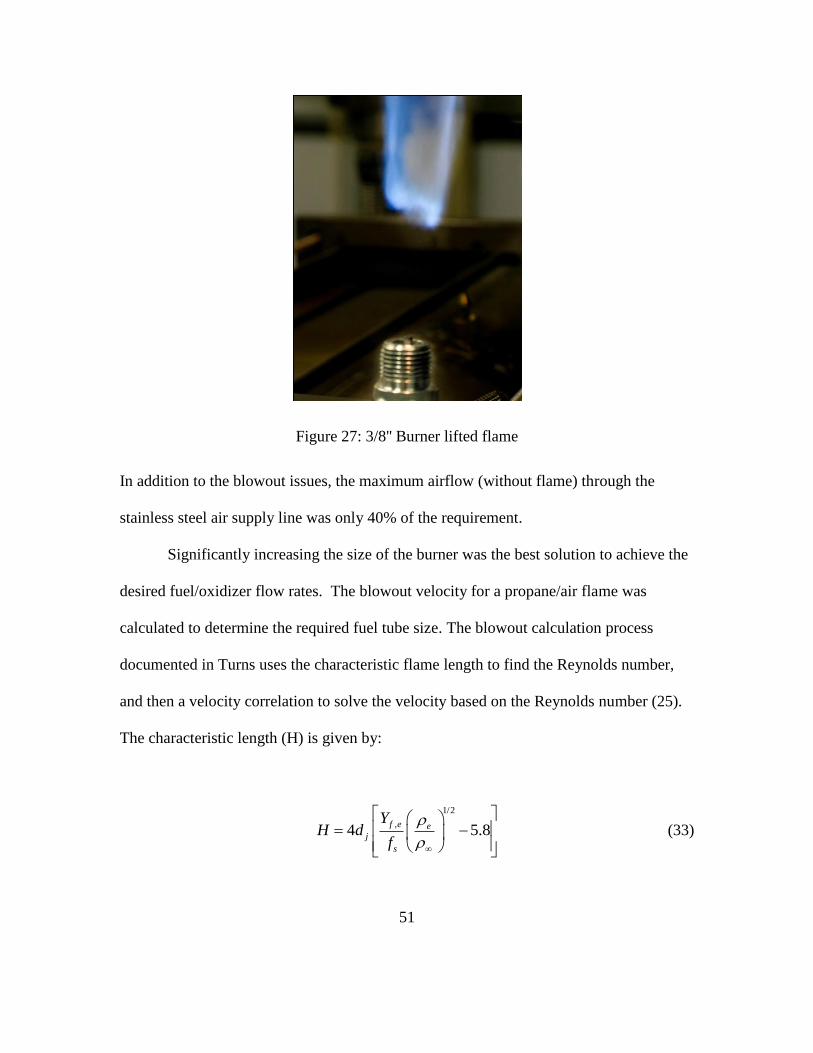
51

Figure 27: 3/8'' Burner lifted flame

In addition to the blowout issues, the maximum airflow (without flame) through the

stainless steel air supply line was only 40% of the requirement.

Significantly increasing the size of the burner was the best solution to achieve the

desired fuel/oxidizer flow rates. The blowout velocity for a propane/air flame was

calculated to determine the required fuel tube size. The blowout calculation process

documented in Turns uses the characteristic flame length to find the Reynolds number,

and then a velocity correlation to solve the velocity based on the Reynolds number (25).

The characteristic length (H) is given by:

1/2

,4 5.8

f e ej

s

YH d

f

(33)

52

where dj is jet diameter, Yf,e is mass fraction at exit (1.0), fs is mixture fraction, ρe is fuel

density at exit, and ρ∞ is room air density. Each variable is known, allowing H to be

solved directly. The Reynolds number (ReH) is:

maxRe eH

e

SL H

(34)

where SLmax is maximum laminar flame speed, and μe is fuel viscosity at exit. The

Reynolds number leads to the blowout velocity in Equation 35:

1.5

6

max 0.017 Re 1 3.5 10 Ree H H

e

v SL

(35)

The blowout velocity for the inner fuel tube is 23.2 m/s, well below the 140 m/s required

for the desired fuel mass flow rate. The first burner blew out at 22.7 m/s, close to

calculated blowout velocity.

A 2‘‘ stainless steel ―T‖ fitting provided the basis for the next iteration of the

burner. A stainless nipple connected the fitting to the inlet wall. The fuel entered

through a ¾‘‘ stainless tube, in the same coaxial fashion as the smaller burner. The fuel

tube was also designed to allow it to either protrude from the burner or be nested inside.

This design can be seen in Figure 28, next to the previous design for comparison.

53

Figure 28: 2'' burner and 3/8'' burner

The blowout velocity for the new fuel tube is 157 m/s, while the propane velocity is only

1.75 m/s. The maximum air velocity was 5.62 m/s (at φ = 0.75). The blowout

calculation does not apply to a premixed or co-axial flow, so the largest fitting size

available was chosen for the new burner design. While the calculation does not directly

apply to co-axial flow, it still gives insight into the behavior of the flame. With the new

design, flow velocity should not be an issue.

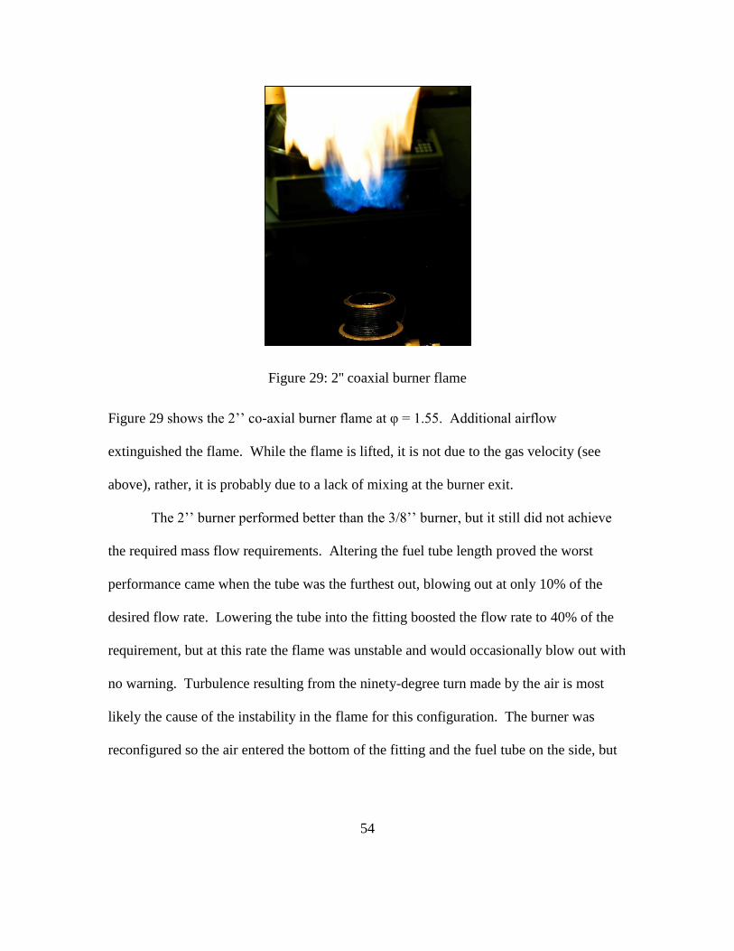
54

Figure 29: 2'' coaxial burner flame

Figure 29 shows the 2‘‘ co-axial burner flame at φ = 1.55. Additional airflow

extinguished the flame. While the flame is lifted, it is not due to the gas velocity (see

above), rather, it is probably due to a lack of mixing at the burner exit.

The 2‘‘ burner performed better than the 3/8‘‘ burner, but it still did not achieve

the required mass flow requirements. Altering the fuel tube length proved the worst

performance came when the tube was the furthest out, blowing out at only 10% of the

desired flow rate. Lowering the tube into the fitting boosted the flow rate to 40% of the

requirement, but at this rate the flame was unstable and would occasionally blow out with

no warning. Turbulence resulting from the ninety-degree turn made by the air is most

likely the cause of the instability in the flame for this configuration. The burner was

reconfigured so the air entered the bottom of the fitting and the fuel tube on the side, but

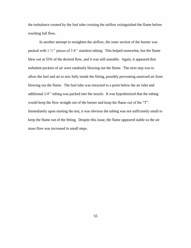
55

the turbulence created by the fuel tube crossing the airflow extinguished the flame before

reaching full flow.

In another attempt to straighten the airflow, the outer section of the burner was

packed with 1 ½‘‘ pieces of 1/4‘‘ stainless tubing. This helped somewhat, but the flame

blew out at 55% of the desired flow, and it was still unstable. Again, it appeared that

turbulent pockets of air were randomly blowing out the flame. The next step was to

allow the fuel and air to mix fully inside the fitting, possibly preventing unmixed air from

blowing out the flame. The fuel tube was retracted to a point below the air inlet and

additional 1/4‘‘ tubing was packed into the nozzle. It was hypothesized that the tubing

would keep the flow straight out of the burner and keep the flame out of the ―T‖.

Immediately upon starting the test, it was obvious the tubing was not sufficiently small to

keep the flame out of the fitting. Despite this issue, the flame appeared stable so the air

mass flow was increased in small steps.

56

Figure 30: 2'' Burner, increasing φ (left to right)

The flame decreased in luminosity and length as the airflow increased. This result was

expected because the flame was changing from a diffusion flame to a pre-mixed flame.

Around 50% of the desired air flow, various parts of the burner began to glow red and the

combustion could be best characterized as violent (loud, very turbulent). Flow was

increased to 100% but by this point the nipple was bright orange, the fitting was bright

red, and the 1/4‘‘ tubing was melting. The component melting along with the general

safety concern from having a violent flame inside the fitting caused this design to fail.

The previous design demonstrated that allowing the fuel and air to mix inside the

fitting would lead to the desired flow rate. By keeping the flame out of the fitting, the

57

melting and safety issues are eliminated. To keep the flame outside the burner body, an

insert was designed for the nipple section. The insert is shown in Figure 31.

Figure 31: Burner insert

Designing the insert involved three considerations:

1. Maximizing the open area to avoid blow-out (minimize velocity)

2. Minimizing the hole size to prevent flashback

3. Factor in machine-ability concerns with the hole size and proximity

As a starting point, the maximum velocity was set to 18 m/s to avoid blowout.

With the mass flow rate and velocity, the total area of all the holes is constant. To

prevent the flame from propagating through the holes, the maximum hole size must be

less than the quenching distance for propane. The minimum quenching distance for

propane is 0.071‘‘ (25); the insert design had 193 holes each with a diameter of .068‘‘.

58

This iteration of the burner design did keep the flame out of the ―T‖, but once

again, the burner was plagues by random blow-outs and instability. The flame did not lift

off, so the gas velocity was not an issue. Based on the theory that a lack of mixing was

causing the blowouts, small stainless steel beads were placed into the nipple (~1.5‘‘ deep)

to encourage mixing. The steel beads in conjunction with the nipple insert finally

allowed full flow combustion with the burner. Despite the apparent solution, the beads

presented a design challenge. In the burner testing, the beads rested in the nipple,

supported by the insert. With the horizontal configuration of the FCR for this testing, the

beads would spill out of the nipple and into the body of the box. There are many possible

solutions to this problem, but most involved the machine shop producing more hardware.

In this case, a simpler solution was to put the ―T‖ upstream of the nipple/insert and allow

the gasses to mix along some length of pipe. The hardware necessary to build a 2‘‘

burner with an 18‘‘ long, 1.5‘‘ mixing pipe was on hand and put to use. No beads are

required when using the mixing tube. Figure 32 shows the final burner configuration

next to the original for comparison.

Figure 32: Final burner configuration

59

Not only did this configuration allow for full flow combustion in a horizontal

position, but it also had the straightest (most laminar) flow of any tested configuration.

Chapter 4 will further discuss the final burner design and flame.

The larger burner diameter forced rebuilding of the inlet walls. The old and new

inner inlet walls (without the cover) are shown in Figure 33.

Figure 33: Old (left) and new (right) inlet wall

In addition to increasing the burner size, the new walls move the flame closer to the test

section and add some material around the window (on the inner wall) to provide a better

seal for the water coolant.

3.3.3 Water Cooling-Heat Flux Measurement

The water-cooling feature of the FCR protects the metal from the hot combustion

environment, along with providing a method to quantify the heat transferred to the rig.

The AFIT labs have built-in coolant lines using a 30% propylene glycol coolant, but plain

tap water was used due to concerns related to fluid loss in the coolant system along with

the environmental issues related to any leaked fluid.

60

Tap water was also chosen because it is convenient and cheap. Garden hoses

connect the source to the inlet manifold and the outlet manifold to the drain. The FCR

leaked at various times in various places, but the leaked water posed no environmental

risk. No pump is required to move the fluid through the system due to the inherent head

pressure at the tap. The main drawback to tap water is its cleanliness. A filter was placed

in-line with the inlet hose to stop large contaminants from fouling the system, but nothing

was done to address hard water build-up. Even after short test runs, calcium carbonate

buildup was evident on the interior of the FCR walls. The small passages in the needle

valves and flow meters are particularly susceptible to the hard water deposits. .

61

Figure 34: Water cooling overview

62

The inlet and outlet water manifolds are not an actual part of the FCR, but are

critical to collecting the heat transfer data desired for the calorimetry experiment. Along

with splitting the flow to each wall, the manifolds measure temperature and flow, and

control flow to each wall.

Figure 35: Inlet manifold

Figure 35 shows the bottom portion of the water-cooling inlet manifold. The top

portion contains a valve and flow sensor for the test section flow. The first component of

the inlet manifold is a 396 gallon-per-hour magnetic-inductive flow sensor,

approximating the observed maximum volumetric flow rate of a standard tap. The flow

meter has a digital display as well as digital and analog output. The analog output (4-20

mA) was wired to the control computer data acquisition system and brought into

LabVIEW®. Next, the water enters a Delrin® (polyoxymethylene plastic) manifold that

splits the flow into seven parts. The incoming temperature was measured using a ―T‖

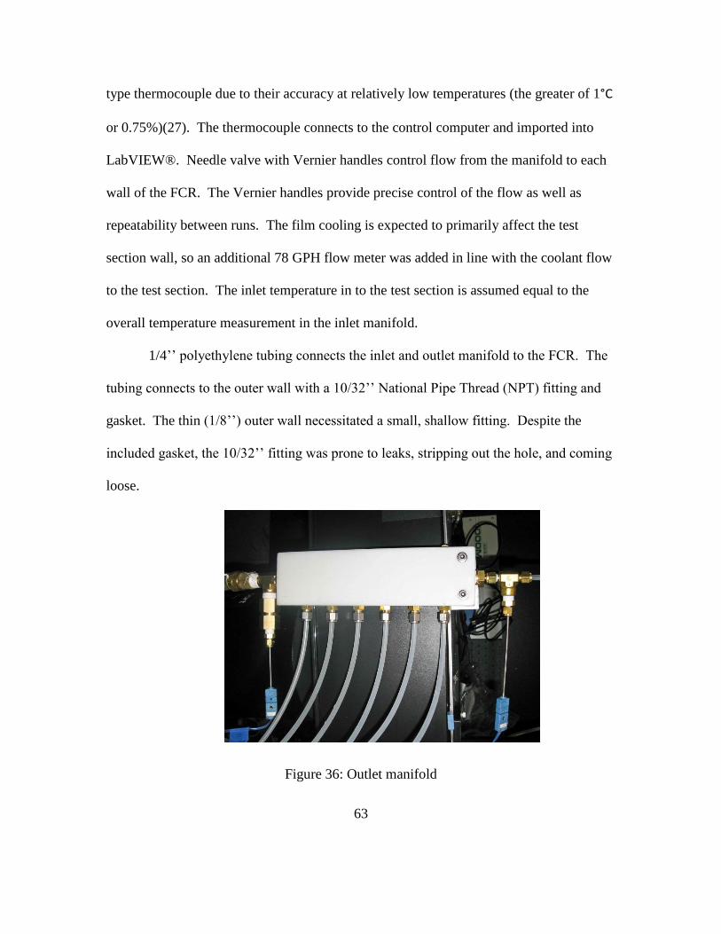
63

type thermocouple due to their accuracy at relatively low temperatures (the greater of 1°C

or 0.75%)(27). The thermocouple connects to the control computer and imported into

LabVIEW®. Needle valve with Vernier handles control flow from the manifold to each

wall of the FCR. The Vernier handles provide precise control of the flow as well as

repeatability between runs. The film cooling is expected to primarily affect the test

section wall, so an additional 78 GPH flow meter was added in line with the coolant flow

to the test section. The inlet temperature in to the test section is assumed equal to the

overall temperature measurement in the inlet manifold.

1/4‘‘ polyethylene tubing connects the inlet and outlet manifold to the FCR. The

tubing connects to the outer wall with a 10/32‘‘ National Pipe Thread (NPT) fitting and

gasket. The thin (1/8‘‘) outer wall necessitated a small, shallow fitting. Despite the

included gasket, the 10/32‘‘ fitting was prone to leaks, stripping out the hole, and coming

loose.

Figure 36: Outlet manifold

64

Figure 36 shows the outlet manifold. The temperature is again measured using

―T‖ thermocouples, but this time it is measured for both the test section and the overall

flow. The seven lines combine into one and then the hot water flows out to a drain built

into the floor of the lab.

Figure 37: Inner wall with RTV applied (not yet sealed)

The other major modification to the system to allow water-cooling was sealing the

cooling walls. Figure 37 shows part of an inner wall with RTV applied to a portion of the

mating surface. A high-temperature silicon RTV gasket sealant intended for automotive

(oil and transmission pan gasket) applications provides the seal between the inner and

outer walls. Once a bead is placed around every mating surface the outer wall is fastened

to the inner wall and the RTV is allowed to fully cure. The screw holes are particularly

vulnerable to leakage and extra sealant was required in these areas. The lessons learned

section describes the procedure for applying the RTV gasket. Even with the best possible

sealant application, leakage will occur at high flow rates. The Vernier handles limited the

65

flow rate to acceptable levels to prevent leakage. The drawback to limiting the water

flow is some minimum flow needs to be maintained to prevent boiling in the walls. Once

the water boils, the temperature is meaningless.

Each panel was tested with flow rates up to 20 gph (gallons per hour). Some

panel had minor leaks, especially around the fittings for the tubes carrying water from/to

the manifolds. Any leaks would be sealed using RTV once the FCR was assembled.

Chapter 4 describes the performance of the heat flux measurement system and the

changes required to operate the FCR.

3.3.4 Other Modifications

A number of smaller changes were also required to prepare the FCR for combustion and

testing. The ignition system for the propane/air mixture came directly from the UCC.

Anderson (18) initially built the igniter assembly, while Lakusta (21) was responsible for

characterizing its operation. The igniter assembly is show in Figure 38.

Figure 38: UCC/FCR igniter

66

The igniter uses an automotive spark plug to ignite an ethylene/air mixture inside the

igniter body. The spark plug is controlled through LabVIEW® while the gasses are

controlled through the MKS mass flow controller panel. The ethylene/air mixture ignites

inside the igniter body and then the flame travels through a 3/8‘‘ tube to the FCR body.

Drenth (22) showed the original igniter tube was quenching the flame and a shorter tube

was more effective. The FCR uses the shortest practical tube length still with the fitting

common to the UCC. Propane ignites quickly so the igniter is not required to sustain a

flame, although testing showed that a steady flame is possible (Figure 39).

Figure 39: Ethylene/air igniter operation

Windows were also necessary for the FCR. The windows would protect the

cameras from the flame, direct the flow of hot combustion gas toward the nozzle and

exhaust system, and stop room air from reaching the fuel-rich combustion gases (thereby

altering the fuel/air mixture in the rig). McCall (2) specified sapphire windows, although

67

previous experience with quartz in the UCC led to its use in the FCR. The quartz

window is shown in Figure 40.

Figure 40: Quartz and zinc selenide (ZnSe) windows

Fiberfrax, a high temperature insulating ceramic paper, initially served as a gasket

on both sides of the window. The UCC used the same Fiberfrax material (1/8‘‘ 970-J)

for gaskets with no issue, but the environment of the FCR led to the gasket combustion.

While the gasket was believed to be a non-combustible material, a call to the

manufacturer revealed the presence of a small amount of organic material serving as a

binder. The representative recommended a slightly different material, where the organic

material was baked out of the product during manufacture. The new product (1/8‘‘ 882-

J) was significantly more fragile, but it no longer caught fire during testing.

3.3.5 Operating Regime

Testing the operating regime of the FCR began once the combustion related

modifications to the FCR completed. The three major questions answered by this testing

are: what are the correct starting conditions for the igniter and burner, what main and

68

coolant flows are necessary to achieve the correct blowing ratios, and what water flow is

required through the cooling channel of the test section.

Drenth (22) gives the igniter settings for the UCC. As originally designed, it was

difficult to achieve a steady flame in the UCC due to the igniter tube length, as discussed

in section 3.3.4. To prevent the same issue in the FCR, the igniter was first tested outside

the FCR, but with the intended length of stainless steel tube attached. The starting

conditions for the igniter are shown in Table 4. The igniter was then tested installed in

the FCR, but without the end caps or test section, and then finally in the complete FCR.

The igniter never failed to start when properly configured.

With the igniter installed and tested, it was time to find the starting conditions for

the main fuel/air mixture and verify the equivalence ratios found during the burner

testing. Testing for the starting conditions was largely a trial and error process, although

the lessons learned during the burner testing certainly aided the process. Two lessons

were particularly valuable. First, there was an upper limit to the starting mass flow rate,

lower than the operating limit. Similarly, the lean starting limit is higher than the

operating limit.4.

From an operations standpoint, the easiest solution would be to start at the

intended operating condition. The burner testing generally proved that the rich case was

more stable then the lean case, so testing inside the FCR began at φ = 1.5 (the richest

intended equivalence ratio). The test plan was to change the air mass flow rate to vary

4 A lean mixture has an equivalence ratio (φ) less than one. A higher lean starting limit means that the FCR

required a richer mixture to start than to operate.

69

the equivalence ratio, and change the propane coolant mass flow rate to vary the blowing

ratio. In this scenario the propane main flow would always be at its upper limit (~19

SLPM). With this in mind, the propane set point was 19 SLPM with the appropriate air

mass flow rate. At this setting the main flow was not attached to the burner, instead the

igniter flame acted as a flame holder for the main flame. Consequently, the main flame

would not stay lit without the igniter. The air flow was reduced by half for the second

test (φ = 3.0), but the rig once again failed to start. During the open-air burner testing

there was no rich limit because the mixture immediately exited into a semi-infinite

reservoir of air, but the FCR restricted the air to whatever was present in the mixture.

Reasoning that the decreased air flow was causing the mixture to reach the rich

flammability limit, the fuel mass flow rate was decreased until the rig started reliably.

The correct starting conditions for the FCR are shown in Table 4.

Table 4: FCR starting conditions

zero air – igniter 12.5 SLPM

ethylene (C2H4) – igniter 1.35 SLPM

propane (C3H8) – burner 12.5 SLPM

lab air – burner 198 SLPM (0.250 kg/min)

propane (C3H8) – coolant N/A

water – test section cooling 10 gph

70

The flame attached to both the burner and the exit nozzle because the flow exited

the FCR with excess fuel. As expected, the outer flame diminished and then disappeared

completely with decreasing φ. The starting flow is less than the test flow conditions so

the fuel and the air should be incrementally increased to the max fuel flow point. If the

air is increased entirely at once then the flame will blow out. If the fuel is increased at

once then the rig reaches an unsteady operating condition at φ = 2.1 where the flame

oscillates between the outside and inside the box. This condition is shown in Figure 41.

Figure 41: Unsteady operation

The final operating condition test was verifying the range of equivalence and

blowing ratios. The air and fuel flow rates were increased incrementally until reaching

the max fuel flow rate at φ = 1.5. Next, we increased the air flow, decreasing the

equivalence ratio. As φ decreased, the interior flame decreased in size, similar to the

open-air tests. At φ = 0.85 the flame detached from the burner and turbulently swirled

around the inside of the FCR. To avoid this condition, the lower test equivalence ratio

needed to remain at 0.90 or greater.

71

With the upper and lower equivalence ratios tested and set, the coolant flow was

determined. Testing verified operation of the FCR with blowing ratios from 0.5 to 1.5.

There was no noticeable change in the main flow or flame. Chapter 4 will discusses the

IR testing of the coolant flow.

3.4 Testing Methodology

Designing the testing methodology goes hand in hand with designing the test rig.

Build issues sometimes drove testing methods, such as when the total heat flux

measurement was abandoned due to issues with the water-cooling in the sidewalls. In

others cases, the tests necessitated changes to the design, such as when the zinc-selenide

window addition to accommodate infrared measurement. In most cases the test

methodology took precedence unless the issues absolutely could not be overcome.

3.4.1 Infrared Surface Temperature Measurement

McCall (2) first performed infrared testing in the FCR for his earlier work. Figure

42 shows the test setup used by McCall.

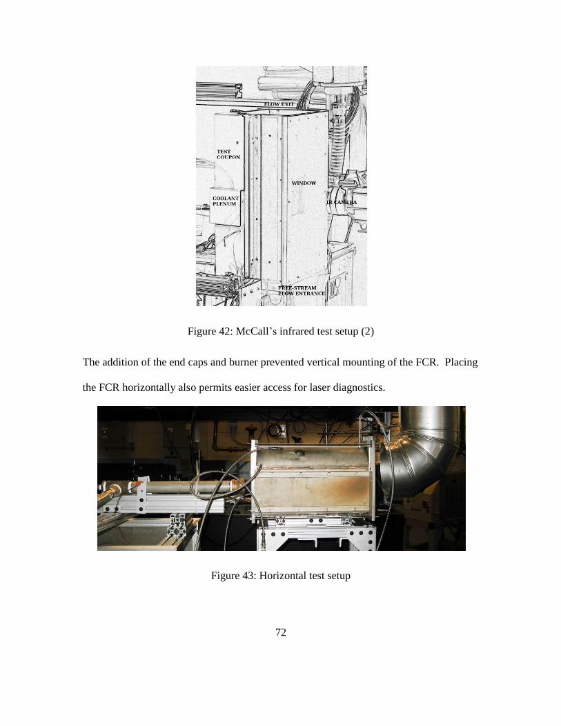
72

Figure 42: McCall‘s infrared test setup (2)

The addition of the end caps and burner prevented vertical mounting of the FCR. Placing

the FCR horizontally also permits easier access for laser diagnostics.

Figure 43: Horizontal test setup

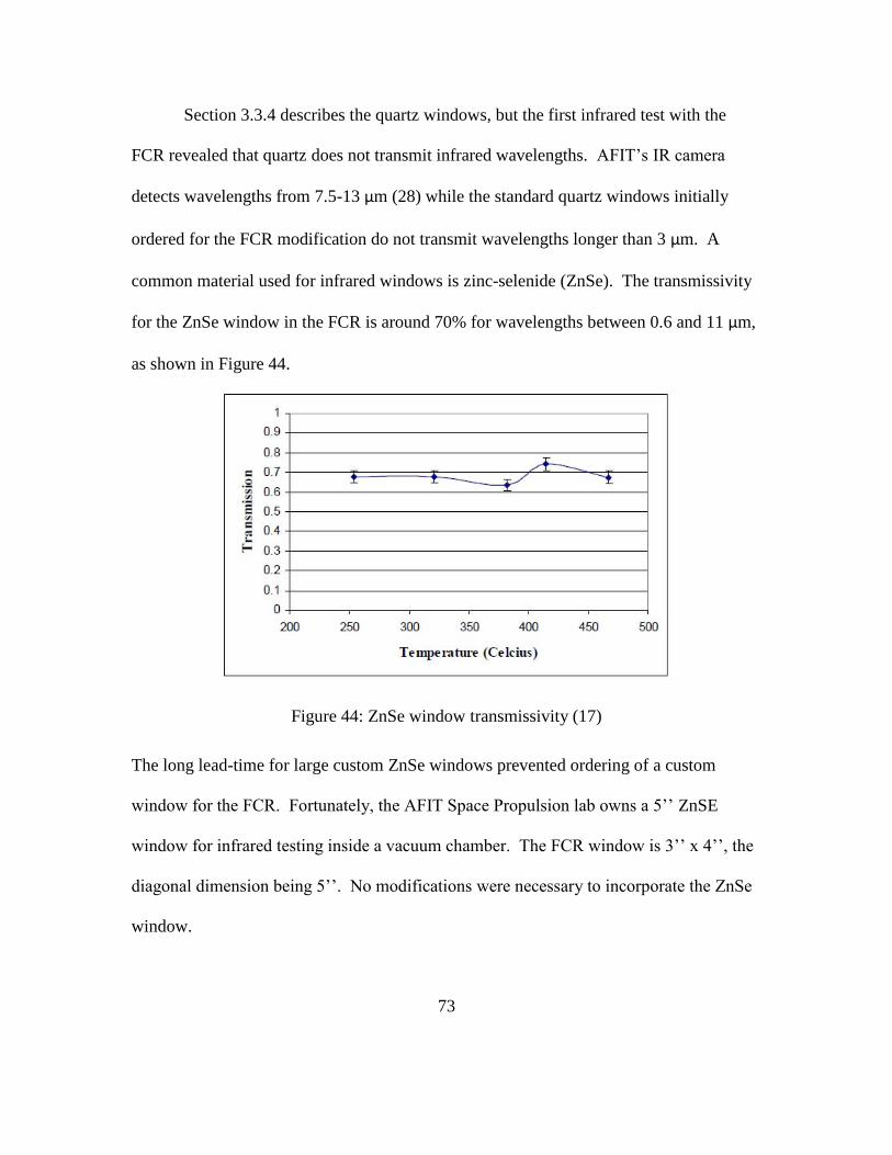
73

Section 3.3.4 describes the quartz windows, but the first infrared test with the

FCR revealed that quartz does not transmit infrared wavelengths. AFIT‘s IR camera

detects wavelengths from 7.5-13 μm (28) while the standard quartz windows initially

ordered for the FCR modification do not transmit wavelengths longer than 3 μm. A

common material used for infrared windows is zinc-selenide (ZnSe). The transmissivity

for the ZnSe window in the FCR is around 70% for wavelengths between 0.6 and 11 μm,

as shown in Figure 44.

Figure 44: ZnSe window transmissivity (17)

The long lead-time for large custom ZnSe windows prevented ordering of a custom

window for the FCR. Fortunately, the AFIT Space Propulsion lab owns a 5‘‘ ZnSE

window for infrared testing inside a vacuum chamber. The FCR window is 3‘‘ x 4‘‘, the

diagonal dimension being 5‘‘. No modifications were necessary to incorporate the ZnSe

window.

74

The second modification to the FCR related to the infrared testing was painting

the test sections. The polished test sections have an emissivity in the range of ~0.18-

0.35, compared with the painted sections emissivity of ~0.95. In practice, this meant that

the polished sections reflected the background temperatures, while the painted sections

emitted more IR radiation.

The long direct exposure to direct flame necessitated high temperature paint. A

variety of products is available for use in engines, furnaces, and stoves. VHT®

Flameproof flat black paint was available online and chosen for the FCR. VHT®

Flameproof is a ceramic spray paint able to withstand temperatures up to 1093°C

(2000°F). Three coats of paint were applied to each test section and allowed to dry

overnight. The instructions give baking times and temperatures to fully cure the paint,

but the air supply hose in the COAL lab could not sustain the required temperatures. In

addition, the un-insulated hose caused the air temperature to drop substantially before

reaching the FCR. At higher upstream temperatures, the hoses started to melt. The

recommendations section gives more information on the high temperature hose issue.

Failure to bake the paint did not seem to affect performance in any way.

75

Figure 45: FLIR systems SC640

The FLIR® Systems IR camera shown in Figure 45 is the same camera used by

Bohnert (17) and McCall (2). Appendix C covers operation of the camera and software.

It is a portable unit, easily hand carried, and somewhat ruggedized. The manufacturer

markets the camera for professional users in the home inspection, electrical, and other

industries. Table 5 lists the specifications of the IR camera.

Table 5: P640 camera properties (17)

The camera distance from the window was approximately 10‘‘. The distance is greater

than McCall‘s to protect the camera from the high heat output of the FCR. In addition,

76

the camera was removed from the setup while not actively testing to avoid heat buildup.

The cost of increasing the distance from the camera to the FCR is a loss of resolution

around the coolant hole region.

For each IR test, the FCR was started, set to φ=1.5, and the rig allowed to reach near

steady-state conditions. Steady-state was defined as less than 2°C temperature change in

the water coolant over 10 minutes. Once at steady state the water temperature data was

recorded and the software commanded to start data acquisition. For each test case 10

seconds of data was recorded at 10 Hz (300 pictures total). The software then converted

the data to a MATLAB® file format. A MATLAB® program (Appendix D) mapped the

picture of the curved section to a 2-D plane and averaged the temperature values.

Recall from Equation 10 that the film cooling efficiency is defined as:

awf

c

T T

T T

For the efficiency to properly vary between 0.0 and 1.0, Taw = T∞ when no cooling is

present and ηf = 0. This condition means T∞ for any pixel is the value of that pixel if no

coolant was present. Similarly, for the perfectly cooled case Taw = Tc, and ηf = 1.0. In

the second case, the wall temperature is the coolant temperature. The camera is

measuring the value of Taw at each pixel location if that pixel is steady-state (adiabatic).

If we assume the temperature of the each pixel is a function of the length from the burner,

then T∞ is obtained from an uncooled test section at the same streamwise location.

Comparison of the water coolant temperature change ensures that the cooled and un-

cooled test cases are for the same conditions.

77

The coolant temperature at the hole exit, Tc, is the toughest variable to solve in

this situation. McCall (2) found that measured temperature at the center of the hole

equaled the coolant temperature obtained with thermocouples inside the cooling plenum.

Without a cooling plenum like McCall, it is difficult to obtain the temperature due to the

small tube area. Chapter 5 describes one possible method to determine the coolant

temperature. This research used the temperature at the center of the coolant hole for the

coolant temperature. Chapter 4 will discuss the results of this assumption.

With all three temperatures from Equation 10 known, ηf is also known at each

pixel location. It is also possible to integrate in the manner of Equations 11 and 12 to

obtain the spanwise and area-averaged efficiency.

3.4.2 Calorimetry

The calorimetry data from the FCR is a byproduct of the water cooling system.

The water flows behind the entire test section, entering near the burner and departing near

the nozzle. The maximum heating from the burner on the test section occurs somewhere

downstream of burner, while the water temperature is increasing constantly as it moves

across the test section. The total temperature change is the only recorded data, permitting

an average heat flux measurement for the entire test section. Film cooling works by

carrying heat away from the surface, and blocking heat from being transferred to the

surface. As the cooling efficiency increases, the heat flux from the test section to the

water coolant should decrease. It is also possible that the rejection of the heat by the film

coolant causes another region to experience more heat. The six flat walls of the FCR

originally included water cooling to capture the total heat flux.

78

The heat added to the water is shown in Equation 36.

(36)(36)

where ΔQ is heat added to the water, is water mass flow rate, cp is the specific heat of

the water, and ΔT is change in water temperature. The heat flux is then the total heat

divided by the interior area of the test section wall:

2Q Q

qA rl

(37)

where A is test section area, r is test section radius, and l is test section length. The

decrease in heat flux will be very small due to a single coolant hole, but future testing

may involve arrays of holes to implement full coverage film cooling. The change in heat

flux due to the coolant hole reinforces the surface temperature measurement by the IR

camera. It may also be useful when the combustion products obscure infrared

measurement of the wall temperature.

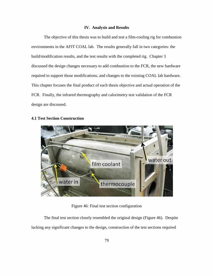
79

IV. Analysis and Results

The objective of this thesis was to build and test a film-cooling rig for combustion

environments in the AFIT COAL lab. The results generally fall in two categories: the

build/modification results, and the test results with the completed rig. Chapter 3

discussed the design changes necessary to add combustion to the FCR, the new hardware

required to support those modifications, and changes to the existing COAL lab hardware.

This chapter focuses the final product of each thesis objective and actual operation of the

FCR. Finally, the infrared thermography and calorimetry test validation of the FCR

design are discussed.

4.1 Test Section Construction

Figure 46: Final test section configuration

The final test section closely resembled the original design (Figure 46). Despite

lacking any significant changes to the design, construction of the test sections required

80

the most time (and money) of any activity in this research. There are currently eight test

articles. Two (one 4‘‘ and one 6‘‘) were welded and machined, but otherwise unfinished.

The unfinished test section allowed development of the operating regime while

production continued on the remaining articles. Two (one 4‘‘ and one 6‘‘) have coolant

holes for 45° compound injection but do not have coolant tubes, thermocouples, and are

not painted. The remaining four test sections (0° and 90° injection, 4‘‘ and 6‘‘ radius)

were completed and used for testing.

The thermocouples in the stainless steel test sections were brazed into place as

discussed in Chapter 3. Prior to brazing, each thermocouple was calibrated using the

same technique as McCall (2). Each thermocouple measured the temperatures of an ice

bath and boiling water, setting the calibration points for 0 °C and 100°C. The linear

curve fit of the calibration points gives the true temperature for any thermocouple

measurement. McCall‘s calibration showed his thermocouples did not have any bias

error beyond the capability of the data acquisition system so calibration curves were not

necessary. Figure 47 shows a portion of the calibration curve for one of the three

thermocouples used in this research. The calibration yields a more accurate temperature

measurement then simply using the manufacturer‘s published error range (shown by the

error bars).

81

Figure 47: Thermocouple error (@20-50 °C). The baseline is where the measured

temperature equals the actual temperature

At very high temperatures (~700°C+) the calibration curve may fall outside of the

manufacturer data, in which case a better calibration method for high temperatures is

required. For the temperature range expected in the FCR (<300°C), every calibration

curve fell inside the manufacturer‘s error range.

McCall (2) corrected the infrared temperature measurement by recording the

infrared temperature of the thermocouple (at the tip) inside the FCR for each test. Each

pixel was adjusted by the difference between the thermocouple and IR measured value.

For example, if the thermocouple read 77°C, and the IR camera 83°C, then each pixel

from the IR camera would be adjusted down 6°C in the same manner as McCall(2). The

plan for this research was to use the same technique, minimizing bias error in the camera

temperature measurement. The major benefit to this method is avoiding the requirement

to find the emissivity, transmissivity, and all the other factors necessary to calibrate the

20

25

30

35

40

45

50

20 25 30 35 40 45 50

Act

ual

Te

mp

era

ture

(C

)

Measured Temperature ( C)

baseline

TC1 (T)

82

camera. Not only does each factor have a contribution to the overall error, but also some

of the factors (atmospheric temperature) change dramatically over the path from the test

section to the camera sensor. The camera settings are not complex enough to cover every

possible test setup.

The first test section produced was a 6‘‘ radius section. The AFIT machine shop

brazed an ―N‖ type thermocouple into the test section using the same technique as for the

coolant tube, except the tip extended approximately 0.135‘‘ into the test section (Figure

48).

Figure 48: Thermocouple extending from test section

The ―N‖ type thermocouple was chosen for its stability at high temperatures compared to

the more common ―K‖ type thermocouple. A handheld device displayed the

thermocouple temperature during the brazing to ensure the thermocouple was not

damaged by the high temperatures of the oxygen-acetylene torch. The maximum

temperature displayed during brazing was 322°C, well below the maximum temperature

rating (1300°C). The tip of the thermocouple was glowing bright red in the direct flame

83

of the brazing torch. The actual temperature was estimated using the color of the glowing

metal. For 316 stainless steel (with a similar melting point as the thermocouple sheath),

the color indicated a temperature well above 500°C (29). The thermocouple is therefore

not reading the temperature at the tip of the sheath (the surface temperature), but rather it

is reading some average temperature of the test section wall. Testing inside the FCR

verified the same result.

With the IR camera temperature calibration by thermocouple in question, the

remaining option was to use the internal camera calibration settings. Chapter 3 covered

the drawbacks to using the internal camera settings. Without a better method of

determining the temperature bias, the calculated efficiency values only allow qualitative

conclusions regarding the cooling efficiency.

4.2 Final Burner Design

After much iteration, the final burner design was a turbulent pre-mixed propane-

air flame. The mostly fuel-rich operating range of the burner resulted in a pre-mixed

inner flame surrounded by a diffusion flame. The excess fuel in the mixture reacting with

the room air created the diffusion flame. Figure 49 shows the diffusion flame growing

with the equivalence ratio.

84

Figure 49: Burner flame in open air, φ increasing left (0.9) to right (1.5)

If the FCR were perfectly sealed, only the pre-mixed flame would exist inside the rig,

while the diffusion flame would exist outside of the rig. The unsealed wall joints allowed

room air to create a small diffusion flame inside the rig. The air supply was limited

enough to force a diffusion flame at the exit of the FCR, as expected of a sealed box.

Figure 50: Diffusion flame at FCR exit

85

The velocity of the gas through the burner limits the low end of the operating

range. The flame base constricts as the airflow increases, probably due to boundary layer

growth inside the mixing pipe. As the boundary layer grows, the air mass must pass

through a smaller effective passage, increasing its velocity further. Eventually the flame

detaches from the burner and either extinguishes or attaches to the nozzle. This in turn

forces the velocity of the air in the middle of the pipe to increase in order to maintain the

same mass flow rate. Figure 51 shows the burner flame narrowing at the base due to the

boundary layer effect.

Figure 51: Burner flame at φ = 0.90

One possible research area for the FCR is relating the equivalence ratio to cooling

effectiveness. Lean main flows combined with a fuel coolant may behave very

differently than rich main flows. Calibrating the air and propane flows is important to

determining the true equivalence ratio. The propane calibration used a BIOS Definer

220, shown in Figure 52.

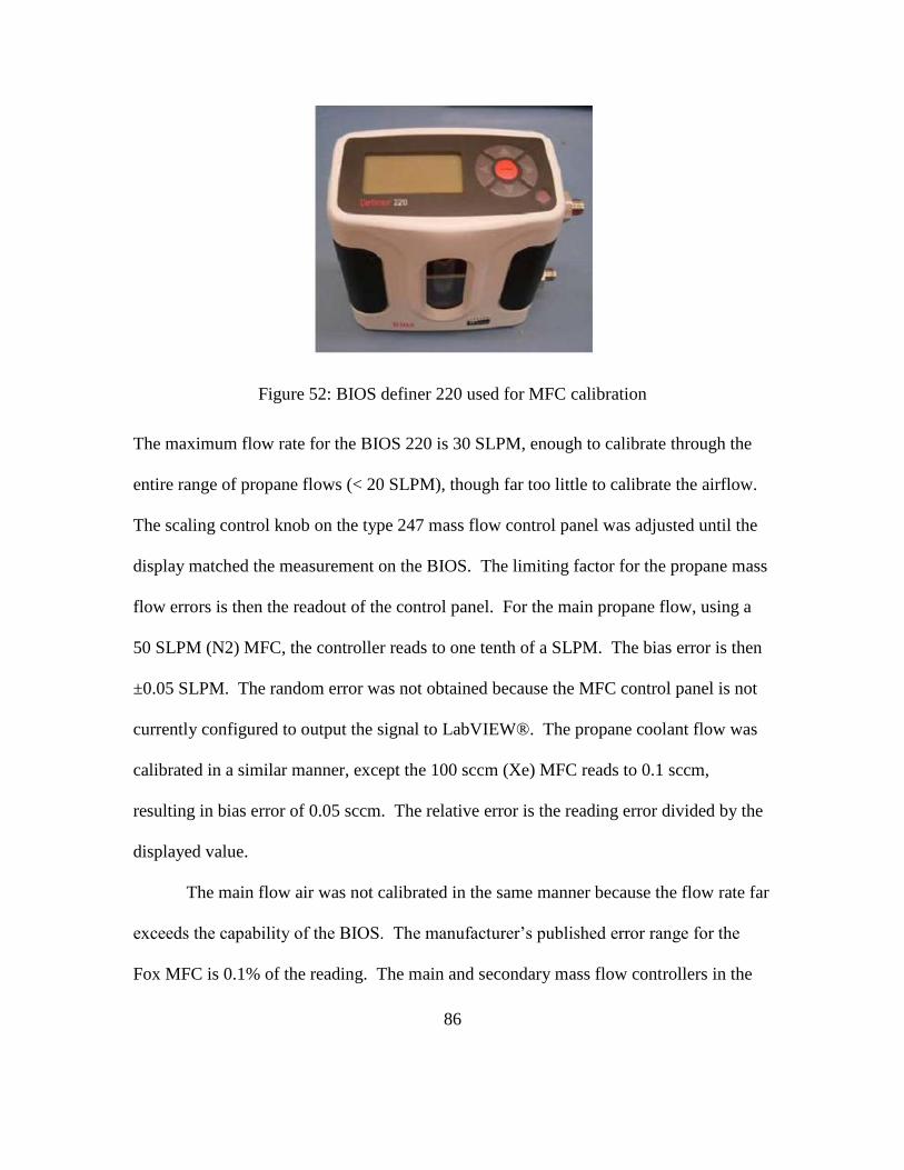
86

Figure 52: BIOS definer 220 used for MFC calibration

The maximum flow rate for the BIOS 220 is 30 SLPM, enough to calibrate through the

entire range of propane flows (< 20 SLPM), though far too little to calibrate the airflow.

The scaling control knob on the type 247 mass flow control panel was adjusted until the

display matched the measurement on the BIOS. The limiting factor for the propane mass

flow errors is then the readout of the control panel. For the main propane flow, using a

50 SLPM (N2) MFC, the controller reads to one tenth of a SLPM. The bias error is then

±0.05 SLPM. The random error was not obtained because the MFC control panel is not

currently configured to output the signal to LabVIEW®. The propane coolant flow was

calibrated in a similar manner, except the 100 sccm (Xe) MFC reads to 0.1 sccm,

resulting in bias error of 0.05 sccm. The relative error is the reading error divided by the

displayed value.

The main flow air was not calibrated in the same manner because the flow rate far

exceeds the capability of the BIOS. The manufacturer‘s published error range for the

Fox MFC is 0.1% of the reading. The main and secondary mass flow controllers in the

87

COAL lab have not been calibrated since installation. Without an adequate calibration

device, it is difficult to determine the bias error, but the random error was obtained using

the signal input to LabVIEW®. It is first important to note the airflow overshoots the

intended value when changed. The airflow was allowed to settle before taking any data

for this research. Figure 53 shows the airflow settling after changing the setting from 0

kg/min to 0.25 kg/min (the startup setting). Minimizing the input changes reduced the

overshoot.

Figure 53: Air flow overshoot and settling when changing flow rate

The airflow oscillates even without the setting changing. Figure 54 shows a three-minute

window of the airflow, 10 minutes after the previous setting change.

0.00

0.05

0.10

0.15

0.20

0.25

0.30

0.35

0 20 40 60 80 100

Mas

s Fl

ow

Rat

e (

kg/m

in)

Time (s)

88

Figure 54: Air flow oscillation at 0.4067 kg/min setting

The airflow was recorded at a sampling rate of approximately 5 Hz for 10 seconds.

Figure 55 shows a typical 10 second airflow sample, where the set point was 0.4067

kg/min (φ = 1.5 for 20 SLPM of C3H8).

Figure 55: Air flow during test window

0.400

0.402

0.404

0.406

0.408

0.410

0.412

0.414

2500 2550 2600 2650

air

mas

s fl

ow

rat

e (

kg/m

in)

time (s)

0.404

0.405

0.406

0.407

0.408

0.409

0.410

2650 2652 2654 2656 2658 2660

air

flo

w r

ate

(kg

/min

)

time (s)

89

The mean flow rate is 0.4078 kg/min with 95% confidence that the true mean is

±0.0817%. The relative error in the equivalence ratio is then the sum of the relative

errors of the propane (0.0025 for 20 SLPM) and the air (0.000817). In this example, the

error in the calculated equivalence ratio (φ = 1.5) is 0.33, or φ = 1.5 ±.005.

4.3 Heat Flux Experiment Design

Implementing the water cooling/heat flux measurement system was one of the first tasks

of this research. Chapter 3 described the water cooling system and the method used to

seal each wall. Once the burner and test sections were ready, the entire FCR was

assembled and run. This section describes the results of the heat flux system testing in

the full FCR and the modifications that resulted.

The testing of the complete heat flux system began with the water flow to each

wall of the FCR set at 10 gph, half the amount tested in the stand-alone panels. No

leakage was immediately apparent, although once the flow increased to 12 gph some

small leaks appeared in multiple panels. This was a much lower flow rate than previous

successful testing. The two main factors in the leakage were probably the orientation of

the panels and the stresses introduced when the panels were connected.

During stand-alone testing, each panel rested horizontally on the test bench with

the inner wall on bottom and the outer wall on top. Only the top panel orientation

matched the test configuration once the FCR was constructed. The four sidewalls sat on

their long end, while the bottom wall was upside down (the outer wall was on bottom)

and supported by a 1 ½‘‘ aluminum T-slot frame. In this orientation, the weight of the

90

water inside the panel presses against the outer wall and the weight of outer wall does not

hold it against the inner wall and gasket.

The second cause of the leakage was the connection between panels. The

stainless steel construction made the weight of each panel significant. With the panels

connected together, the weight was focused at the joints, instead of distributed across the

inner wall in the stand-alone testing. The result was some bending and twisting of the

panels once assembled.

Together, these two factors limited the maximum water flow to 10 gph in the

assembled FCR. Once heat was added however, even 10 gph caused sustained leakage.

As the rig temperature increased, the leakage increased. As water leaked from the

sidewalls it seeped into the cracks between the walls and then into the rig, contaminating

the flame. In addition, the seals around the windows leaked profusely, clouding the

windows with mineral deposits (from the hard water). The changes necessary to

implement this water cooling/heat flux measurement system would require almost an

entire rebuild of the FCR. Rebuilding the FCR was not an option, so testing began

without any water cooling.

The existing two-piece walls could not withstand the heat output of the burner.

There were once again two contributing factors. First, each inner wall was machined

from 1/2‘‘ thick 316 stainless steel. The outer wall was 1/8‘‘ thick 316 stainless steel.

1/8‘‘ was removed from the inner wall to hold the outer wall. Another 1/4‘‘ was

removed to form the coolant channel. Only 1/8‘‘ of material remained for most the side

wall area. Such a small amount of material could not conduct heat from the hot regions

91

to the cooler regions fast enough to avoid damage. Figure 56 shows the inner wall

construction.

Figure 56: CAD drawing of walls for water cooling

The exit wall was the hottest section because the burner flame directly impinged

on the inner wall and the outer flame attached to the exit nozzle. The window side wall

and top wall also began to glow red-hot during relatively short test runs. Figure 57 shows

the dramatic red glow from the exit panel, indicating temperatures over 800°C (1500 °F).

Figure 57: Inner (right) and outer (left) view of red-hot exit panel

92

The exit panel also warped inward (see the circled region of Figure 57). Eventually the

screws holding the exit panel window frame popped out of the panel. The second

contributing factor to the failure of the hollow walls was that without fluid movement

through the cooling channels, the air inside the channel insulates the inner panel so the

heat cannot radiate to the surrounding environment. Removing the outer panels could

mitigate this effect, but it introduces a completely new set of design challenges and still

fails to solve the problem (the wall in Figure 57 did not have the outer wall attached).

The only remaining option was to rebuild the walls. Time constraints prevented

construction of improved water-cooled walls, but simple 1/2‘‘ thick solid walls required

much less effort by the machine shop. The exit and the window sidewalls were the main

priorities because they showed the highest heating during the test run. New solid top and

small side walls for the 4‘‘ test sections were also constructed, as McCall‘s (2)walls were

incorrectly sized. The original bottom, inlet, and small sidewalls for the 6‘‘ section

remained, with no adverse effects. Figure 58 shows an old (hollow) and a new (solid)

sidewall.

93

Figure 58: Solid (top) and hollow (bottom) small side walls for the 4‘‘ test section

The schedule savings are a result of not requiring milling of the cooling channel,

manufacture of the outer wall, or drilling and tapping the numerous screw holes. The

original walls took a few days each to complete while multiple solid walls took only in a

few hours. Test runs with the solid walls showed no signs of warping; glowing due to

elevated temperatures was limited to small regions around the exit nozzle (Figure 59).

Figure 59: Solid exit wall nozzle

94

The drawback to using solid walls was losing the ability to measure the total heat

flux on the FCR. This was acceptable because any changes in the heat flux are most

pronounced on the test section with the coolant hole. Film cooling prevents heat from

reaching the wall, possibly causing increased heat flux to un-cooled regions. In this

experiment, with a single coolant hole, any change in heat flux to the un-cooled panels

would most likely be lost in the noise of the total heat flux.

In addition to simplifying the walls, abandoning water-cooling for the side panels

simplified the water manifold setup. Figure 60 shows the new manifold setup.

Figure 60: New inlet (left) and outlet (right) water-cooling manifolds

With water only flowing to the test section, the new manifolds are not actually manifolds

at all. The terminology remains the same because they perform the same functions as the

original manifolds: measuring temperatures and flow rate. Future FCR designs may

incorporate the original manifolds.

The water flow rate to the test section was constant throughout the experiment. A

flow rate of 10 gph allowed an adequate temperature change without boiling. The

95

polyethylene tubing started to leak at the connection to the test section so stainless steel

tubing replaced it with no sign of leakage.

Figure 61: Water temperature change for complete test

Figure 61 shows the change in water temperature for one test run (measured at the

inlet and outlet manifolds). The data collection occurred at the end of the run (from t =

2650-2660 s). It is unknown why the temperature periodically spiked, or why there was

so much variation in the data at the end of the test. The temperature spikes and noise did

not correspond to simultaneous changes in the air or water flow rates.

0.0

5.0

10.0

15.0

20.0

25.0

30.0

0 500 1000 1500 2000 2500

De

lta

T, °

C

Time, seconds

96

After the water temperature reached steady state, the IR camera and water

temperature values were recorded near-simultaneously5 for 10 seconds. Figure 62 shows

the change in water temperature during data collection for one test run.

Figure 62: Water temperature change during IR data collection

The mean temperature change in this example was 26.77 °C, with a 95% confidence that

the true mean is 26.77°C ± 0.19%. The thermocouples were calibrated using the

technique described earlier. LabVIEW® simultaneously collected the water flow rates as

shown in Figure 63

5 The test operator starts the camera recording by pressing F5 on the camera control computer and then

presses a button in LabVIEW to start the water temperature, water flow, and airflow recording. A fraction

of a second elapses between the two events.

26.4

26.5

26.6

26.7

26.8

26.9

27.0

27.1

27.2

2648 2650 2652 2654 2656 2658 2660 2662

tem

pe

ratu

re (

C)

time (s)

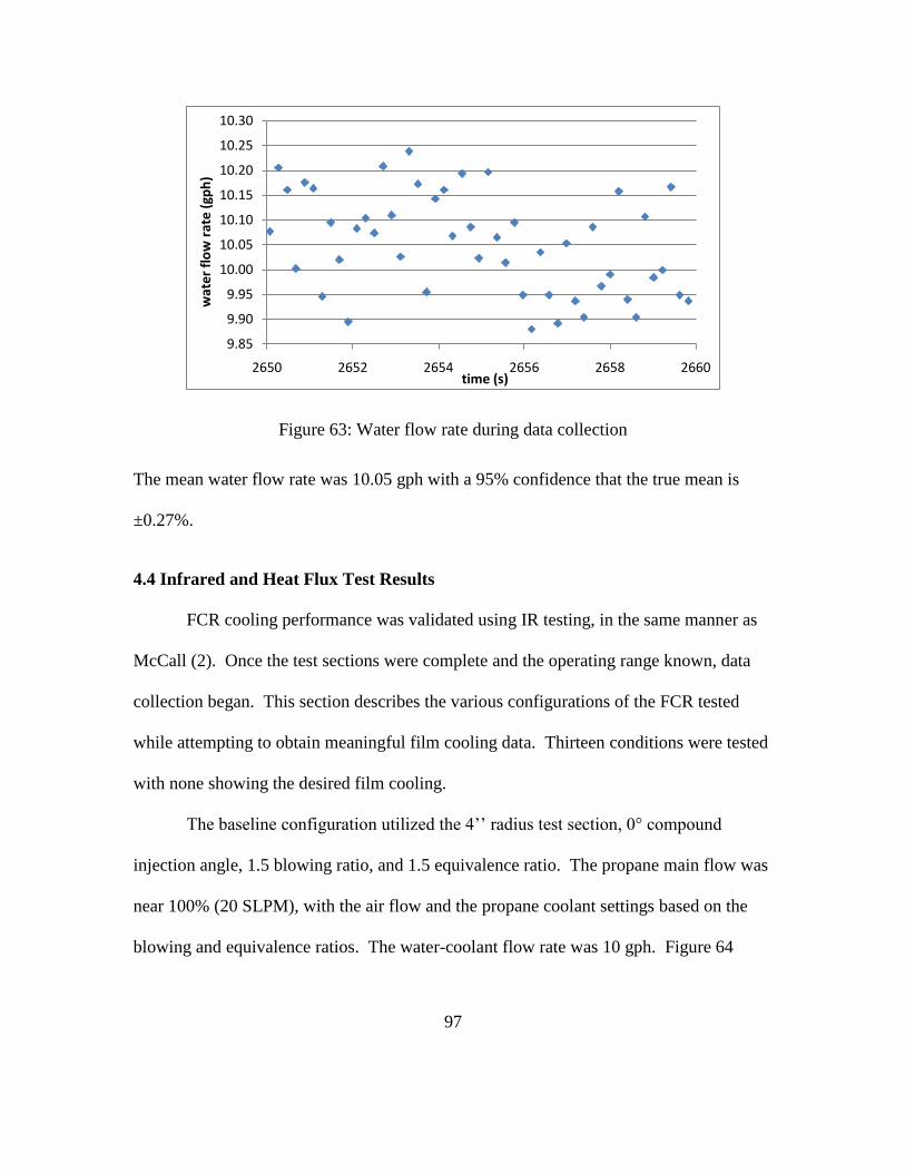
97

Figure 63: Water flow rate during data collection

The mean water flow rate was 10.05 gph with a 95% confidence that the true mean is

±0.27%.

4.4 Infrared and Heat Flux Test Results

FCR cooling performance was validated using IR testing, in the same manner as

McCall (2). Once the test sections were complete and the operating range known, data

collection began. This section describes the various configurations of the FCR tested

while attempting to obtain meaningful film cooling data. Thirteen conditions were tested

with none showing the desired film cooling.

The baseline configuration utilized the 4‘‘ radius test section, 0° compound

injection angle, 1.5 blowing ratio, and 1.5 equivalence ratio. The propane main flow was

near 100% (20 SLPM), with the air flow and the propane coolant settings based on the

blowing and equivalence ratios. The water-coolant flow rate was 10 gph. Figure 64

9.85

9.90

9.95

10.00

10.05

10.10

10.15

10.20

10.25

10.30

2650 2652 2654 2656 2658 2660

wat

er

flo

w r

ate

(gp

h)

time (s)

98

shows the coolant hole region for one time step. The temperature color range was

optimized to show the coolant hole.

Figure 64: IR camera view of cooling hole (BR = 1.5). Main flow from right to left.

The dark region at the top of the picture is a result of the test section curving

toward the camera. The coolant hole is actually near the middle of the curve, but it

appears at the top when viewed from the camera. The wall of the coolant tube is barely

visible, and the brazing has not affected the wall temperature in the region of the cooling

hole. The temperature is the hottest at the bottom of the picture (for Figures 64-66, and

70), closer to the burner flame.

Initially, two issues arose. First, the temperature fluctuated rapidly across the test

section from frame to frame. It is unlikely the metal is changing temperature at that

speed, but rather the combustion products are either emitting or absorbing infrared energy

as they pass between the window and the wall. This issue will be discussed in more

detail later.

99

The second problem is the lack of any trace of film cooling on the test section

wall. Figure 65 shows the coolant hole region after the curve was flattened and the 300

pictures averaged in MATLAB®.

Figure 65: MATLAB® Averaged temperatures, 0° injection, BR = 1.5 (temperature in

Kelvin). Main flow from right to left.

The hole is visible and cooler than the surrounding material, but the typical

cooling tail streaming from the hole is not evident. Without any downstream effect, the

cooling effectiveness is not measureable.

The 90° compound injection was tested next, because it previously showed better

cooling effectiveness. In addition, the 90° orientation blows coolant down onto the test

section in the region more closely perpendicular to the camera. The MATLAB® code

interpolates the camera data to stretch the top region, meaning the pixel size is greater at

the top than the bottom (less fidelity at top). Despite these two advantages of the 90° test

section, multiple test runs demonstrated no cooling effect for this configuration either.

The 6‘‘ test section has the same benefits as the 90° injection: better expected

cooling efficiency and better wall visibility for the camera. The expectation was for the

100

larger radius to allow the coolant to spread more than the tighter radius, although the

length of the coolant stream may decrease. Testing showed no cooling effect for the 6‘‘

test section.

The blowing ratio has a direct effect on the cooling effectiveness, so it was varied

in an attempt to collect data. First, the test range of 0.5 to 1.5 was attempted, with no

results. Next, the blowing ratio was decreased to 0.1, in case the main flow velocity was

too low to turn the coolant flow, and the coolant was jetting out into the main flow.

Again, no cooling was visible. Figure 66 shows the 0.5 blowing ratio test with no

evidence of film cooling and a similar temperature pattern as the 1.5 blowing ratio test

(Figure 65).

Figure 66: 0° injection, BR = 0.5 (temperature in Kelvin). Main flow from right to left.

Finally, a five SLPM (N2) MFC was installed (50X larger), allowing orders of

magnitude greater blowing ratios. No cooling was observed for blowing ratios of 15 or

150. To verify propane was actually reaching the test section, the propane line was tested

Coolant Hole Diameters

Coola

nt Ho

le Dia

meter

s

1 2 3 4 5 6 7 8 9 10 11 12 13 14

1

2

3

4

5

6

438

440

442

444

446

448

450

452

454

456

458

460

101

in open air. Figure 67 shows the propane flame using the original 100 sccm (Xe) MFC at

100%, equivalent to a blowing ratio of 2.24 for the baseline configuration.

Figure 67 shows just how little propane is flowing through the coolant line. The

tube in the figure is the same size as the coolant tube (0.125‘‘) and the flame is

approximately twice that height (~0.25‘‘).

Figure 67: Propane flame from coolant line

The coolant flow was also tested inside the FCR, using the larger MFC and the coolant

flow for an ostensible blowing ratio of 150. Figure 68 shows the resulting flame from the

propane coolant.

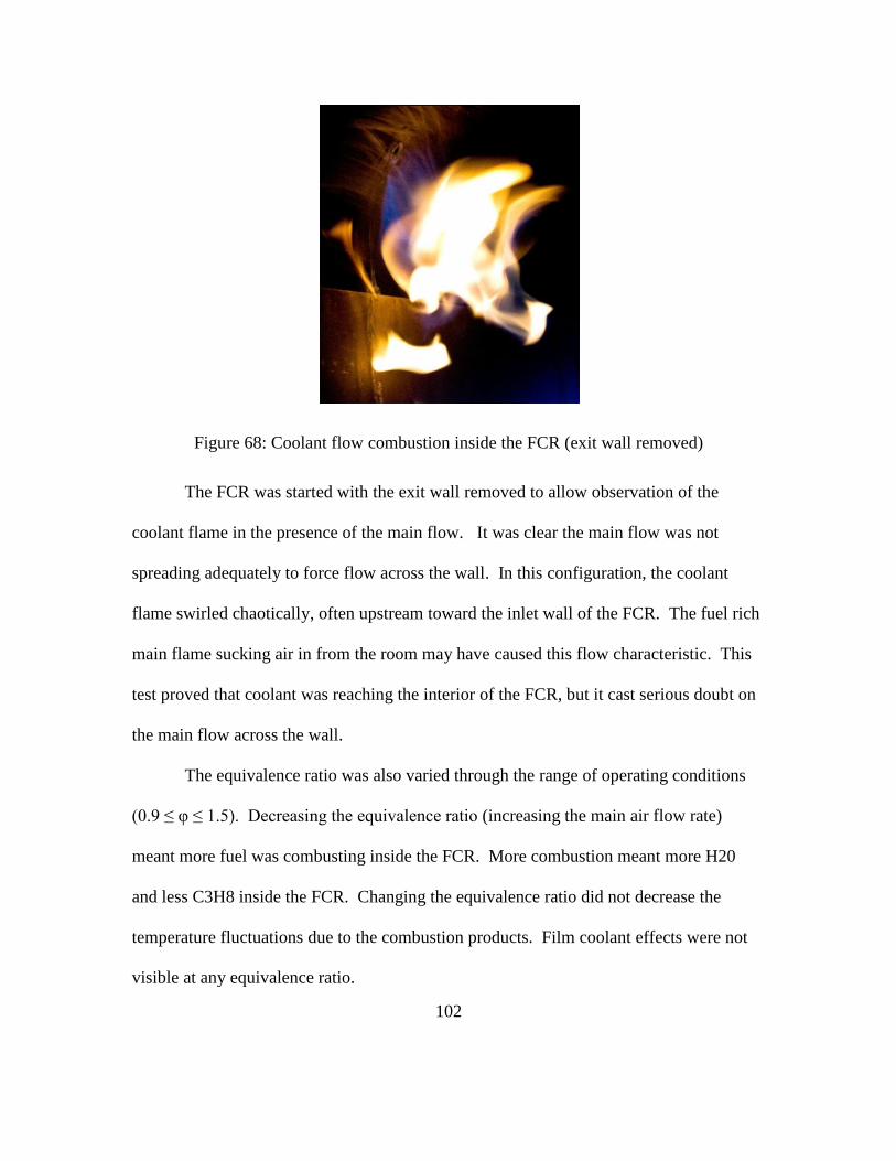
102

Figure 68: Coolant flow combustion inside the FCR (exit wall removed)

The FCR was started with the exit wall removed to allow observation of the

coolant flame in the presence of the main flow. It was clear the main flow was not

spreading adequately to force flow across the wall. In this configuration, the coolant

flame swirled chaotically, often upstream toward the inlet wall of the FCR. The fuel rich

main flame sucking air in from the room may have caused this flow characteristic. This

test proved that coolant was reaching the interior of the FCR, but it cast serious doubt on

the main flow across the wall.

The equivalence ratio was also varied through the range of operating conditions

(0.9 ≤ φ ≤ 1.5). Decreasing the equivalence ratio (increasing the main air flow rate)

meant more fuel was combusting inside the FCR. More combustion meant more H20

and less C3H8 inside the FCR. Changing the equivalence ratio did not decrease the

temperature fluctuations due to the combustion products. Film coolant effects were not

visible at any equivalence ratio.

103

With the full range of normal operating conditions exhausted and no apparent

cooling flow, testing of new configurations and operating conditions ensued. The

primary motivation was getting adequate main flow across the wall. The first option

replaced the nozzle end of the FCR with the stainless steel frame shown in Figure 69.

Figure 69: Open exit wall

This variation attempted to minimize any turbulence caused by the flow

impinging on the exit wall and then wrapping around to the nozzle. The drawback to this

design was room air interacting with the main flow inside the FCR, creating an unknown

equivalence ratio at the coolant hole. A diffusion flame starting at the end of the pre-

mixed flame and extended out of the FCR. Despite the larger exit area, the main flow did

not spread to the wall and the IR camera did not show film cooling near the coolant hole.

Figure 70 shows the open end test case.

104

Figure 70: 90° injection, BR 1.5, open end (temperature in Kelvin)

The coolant hole does not appear clearly as in the previous pictures for two

reasons. First, the braze attempt is much rougher in this test section. Second, there was a

slight leak from the coolant hole, resulting in calcium carbonate build up below the hole.

The leak was remedied as previously described, but minerals from the leak appear as hot

spots in the IR pictures.

Another attempt utilized a wedge insert, used by McCall (2) for pressure gradient

testing, to direct the flow up toward the test section wall. The apex of the wedge sat just

before the coolant hole in the streamwise direction and out of view of the camera. The

burner flame directly impinged on the wedge, heating it to over 800 °C; a wave of flame

was visible over the top of the wedge near the coolant hole. Once again, there was no

trace of coolant flow on the wall.

The next attempt addressed the possibility of the film coolant temperature rising

before reaching the test section wall, therefore not cooling the wall. Without a

thermocouple in the coolant line, it is difficult to correctly assess the coolant temperature,

Coolant Hole Diameters

Coola

nt Ho

le Di

amete

rs

1 2 3 4 5 6 7 8 9 10 11 12 13 14

1

2

3

4

5

428

430

432

434

436

438

440

442

444

446

448

450

105

as previously discussed. One possible solution was increasing the water flow to lower

temperatures surrounding the coolant line and lower the wall temperature. Once again,

no film cooling was visible using a 30 gph (3X) water coolant flow.

In another attempt to address the temperature variations of the combustion

products, the rig was tested using only hot air in the main flow. Figure 71 shows the

temperature variation for a single pixel, both with and without combustion. The error for

the combustion case was 0.093% (0.43°K) while the error for the non-combustion case

was 0.023% (0.093 °K). The temperature error in the combustion case was nearly 4X

greater than the non-combustion case. Despite the obvious difference in temperature

fluctuation for the combustion case, the large sample size yields a very small error and

makes infrared thermography a viable option for both conditions.

Figure 71: Wall temperature variation for a single pixel, with and without combustion

350

370

390

410

430

450

470

490

0 1 2 3 4 5 6 7

tem

pe

ratu

re (

K)

time (s)

With Combustion

Without Combustion

106

In the no combustion test, the air temperature was set to 600°F in LabVIEW®,

with the temperature at the burner exit considerably less. Heat is lost from the poorly

insulated pipes running from the heater to the test stand, from the uninsulated hoses

running to the burner, and from the 18‘‘ burner mixing tube. The burner is not equipped

with thermocouples to measure incoming or outgoing gas temperatures. Once again, no

coolant flow was observed on the wall. Varying the coolant flow from 0% to 100% did

result in the temperature inside the hole decreasing, the first notable effect of cooling

inside the FCR. This test further reinforced the assumption that inadequate main flow

velocity along the test section wall was causing the coolant flow to jet into the main flow

without adhering to the wall.

All attempts to capture film cooling along the test section wall were unsuccessful.

The single largest factor was a lack of main flow velocity along the test section wall. The

temperature variation caused by the combustion products was statistically insignificant

with a sample size of 300. Thirteen different configurations were tested in the attempt to

demonstrate film cooling with many more minor variations not described above. Chapter

5 will discuss the viability of the FCR for combustion testing of film cooling and also

gives recommendations for future testing.

107

V. Conclusions and Recommendations

5.1 Conclusions of Research

This research has shown that the FCR is not viable for film cooling research in its

current configuration using gaseous coolants. Despite successfully completing three of

the four primary objectives, basic design flaws prevent combustion-based film cooling

research in the FCR. The four research objectives are reviewed next, followed by

recommendations for future modifications, and future research.

5.1.1 Curved Test Section Design and Build

The previous researcher left behind a clear design for the stainless steel test

sections. The only undefined features were the coolant tube and the instrumentation

(thermocouples). The combustion environment and stainless steel construction

complicated both features, but the most significant challenge was actually building the

test sections themselves. The pitfall in a complicated component design is that it does not

allow rapid prototyping, testing, and redesign. In this case, only one attempt was

possible, and even that was a challenge. Brazing the coolant tubes was effective at

delivering gas coolant to the test section wall, although brazing required both skill and

practice to accomplish effectively. The thermocouple did not read the surface

temperature as intended. The camera software settings were an acceptable means of

obtaining the test section temperature only because the cooling efficiency equation relies

only on temperature difference and not absolute values. Even had cooling flow been

obtained, this limitation represented a significant weakness in the FCR design. The

108

recommendations section discusses changes to simplify the test section design and

possible temperature calibration methods.

5.1.2 Burner Design and Build

Starting only with a 1/4‘‘ hole tapped into the inlet wall of the FCR and no burner

plans, this research designed, built, and tested a 2‘‘ premixed burner capable of operation

from 0.9 ≤ φ ≤ 2.0+. A co-axial design was originally designed and built, but open air

testing proved that it was not viable without significant additional design effort. A

coaxial design is preferable due to its use in actual rocket engines, but the pre-mixed

burner was simple, stable, and provided the heat and combustion products necessary for

this research. The flame from the 2‘‘ burner did not adequately spread and provide the

hot combustion flow along the test section as intended. The main flow characteristic is

critical to film cooling research so this flaw prevented collection of cooling data. The

recommendations section will describe in detail changes to resolve the main flow issue.

5.1.3 Heat Flux System Design and Build

This research successfully implemented a heat flux measurement system for the

curved test section of the FCR, but failed to demonstrate total heat flux measurement for

the FCR. The heat flux system measured the volumetric flow rate and temperature

change of water flowing over the known area of the test section. LabVIEW® sampled

and recorded these measurements to allow calculation of the average heat flux to the test

section wall. The inability of the FCR to produce film cooling on the test section wall

prevented demonstration of cooling with the heat flux system. For a single coolant hole

in a large test section, the water temperature change due to the film coolant may be lost in

109

the signal noise. The recommendations section discusses changes to heat flux

measurement to allow total heat flux measurement, as originally designed for the FCR.

5.1.4 Operating Regime Design and Test

With the test sections, burner, and heat flux measurement system complete, FCR

operation was demonstrated using the existing COAL lab fuel, air, and control systems.

Simple modifications allowed direct connection of the ethylene/air torch previously

designed for the UCC. The starting conditions for the torch and main burner were

found, as well as the operating range for the FCR with propane/air combustion. Coolant

mass flows equivalent to a blowing ratio range of 0.5 to 1.5 were demonstrated, although

lacking the corresponding film cooling effects due to the coolant jetting into the main

flow. The failure of the coolant to turn and adhere to the wall is due to inadequate main

flow velocity, as previously discussed.

The next section gives recommendations for the issues discussed here as well as

other issues. With these recommendations, the AFIT COAL laboratory is ready to

continue film and effusion cooling research for rocket engine applications. Despite the

lack of measureable data, this research leaves behind a significant amount of knowledge

and lessons learned for future projects.

5.2 Recommendations

Due to inadequacy of the current FCR design, it is appropriate to include a

detailed list of recommendations for future researchers. The first section covers

recommendations for modification to the current FCR. These recommendations are

intended to correct the main flow velocity, allow measurement of the total heat flux, and

110

generally improve the characterization of the operating environment. The second section

discusses a new FCR design that addresses many of the issues with the current design.

5.2.1 Recommendations to Improve the Current FCR

Correcting the main flow velocity along the test section wall must be the main

concern for any future research involving the FCR. This correction may be accomplished

by moving the location of the burner much closer to the test section wall, or changing the

design of the burner so that it incorporates more of the area of the inlet wall.

If the existing burner design is moved closer to the test section wall, then the main

flow combustion gases will travel along the wall, forcing the coolant to turn and cool the

wall. One drawback to moving the burner location is the laser diagnostics access window

location. The window is situated between the burner and test section. The current

window is 3‘‘X4‘‘, much larger than necessary to study the coolant effects along the

wall. For laser diagnostics of the film coolant region alone, a much smaller window is

suggested. The inlet wall must be rebuilt to incorporate these changes.

Another possibility is rebuilding the entire inlet wall to incorporate a burner over

most of the wall area. This more closely resembles a rocket engine combustion chamber

where the inlet end of the chamber mostly consists of fuel and oxidizer injectors. If

possible, the new burner design should include impinging air and fuel jets, resulting in a

diffusion flame inside the FCR. This change would also bring the FCR more in line with

actual engine design, but would require additional effort to design the injection angles,

flow rates and hole spacing. Fabrication issues with such an assembly would also add to

the design challenge.

111

Once the new burner is built, the flow velocity should be tested inside the FCR

(along the test section wall) using hot wire anemometry or PIV. The fragile hot wire

anemometry instruments would probably not survive the combustion environment so hot

air could be substituted for combustion gases to complete the test. The current

LabVIEW® readout for the air temperatures does not reflect the true temperature of the

air at the input to the FCR, so type ―T‖ thermocouples should be added at the junction of

the air/fuel lines to the burner and at the end of the burner. High temperature stainless

steel hosing should be used to connect to the air supply and it should be insulated as

much as practical. Flow velocity testing could be accomplished using the existing test

section walls.

The basic test section design is sound, while some changes may improve the data.

First, omitting the cooling channel will greatly simplify construction of the test sections.

The value of the heat flux data is much less than the infrared surface temperature data or

the laser diagnostic data and removing it solves a number of problems. Without a cooling

channel, it is possible to implement some kind of cooling plenum in the manner

previously described by McCall (2). A cooling plenum simplifies manufacture of the

coolant hole, eliminating the need for a coolant tube or brazing while a single wall can be

machined using traditional mechanical tools and not the EDM used for this research. The

plenum may also allow direct measurement of the cooling flow close to the injection

point.

Another change to the test section should be moving the coolant hole. First, the

hole should be located so the wall near the hole is as close to perpendicular to the camera

112

as possible. The resulting hole will be near the bottom of the test section, and should be

oriented so the coolant flows up the wall when there is compound injection. The hole

should also be moved toward the exit end of the FCR. Moving the hole should result in a

thicker boundary layer, improving the cooling results. Moving the hole location will

require rebuilding of the large side wall, although the test sections could be reused. The

new wall could incorporate the current 5‘‘ ZnSe window, or a new window could be

ordered in the current size (3‘‘ X 4‘‘).

Finally, thermocouple calibration is preferable to relying on the camera settings

for absolute temperature measurement. This research used sheathed, ungrounded

thermocouples. Sheathed-grounded, sheathed-exposed, and bare wire thermocouples

should be tested. The thermocouples may not need to be brazed into the section to

calibrate the camera readings. The thermocouple could be independent of the test

section, but close enough to be in focus when viewing the test section wall.

One change related neither directly to the test section or the burner is the addition

of a gasket or other seal to every wall joint in the FCR. The diffusion flame inside the

current FCR resulted from sucking outside air into the rig. At times, a flame could even

be seen at the corner of the large side wall and the exit wall. Any gasket must be capable

of surviving the intense heat environment. The Fiberfrax® currently employed to seal

the windows may be adequate, but it may alter the fit enough to require rebuilding of

every wall. Properly seating the gasket on every joint will be difficult, and greatly

complicates changing out test sections.

113

In general, further heat flux data collection is not recommended for the reasons

already mentioned. Should the heat flux data be necessary to support the IR data then the

current design may serve as a starting point. Leakage in the FCR walls prevented water

cooling from being included. This leakage effect could be overcome by properly

designing the inner walls and inserts. The lip where the screws attach the two walls and

where the other wall rests should be at least 0.5‘‘ (preferably 1‘‘). This width allows

RTV gasket material to seal the two surfaces together without leaking. The screw holes

should be no more than 2-3‘‘ apart, providing uniform pressure to the seal, and

preventing the outer walls from warping.

Another change to the heat flux system would be to incorporate a reservoir and

pump to allow clean water or some coolant to flow through the lines. The current setup

using tap water will eventually destroy all the equipment. A pump and reservoir would

circulate coolant in and out of the test section. The reservoir needs to be large enough to

prevent the coolant temperature from rising unacceptably due to the recirculation of

heated coolant.

The final recommendations for the existing setup covers the hardware used to

regulate and measure the environment inside the FCR. The most significant change is

adding a mass flow controller capable of regulating the burner airflow. The current setup

using a flow meter, pneumatic valve, and control loop does not match the accuracy of the

other equipment in the laboratory and fluctuations may affect test data at low flow rates.

A larger volumetric calibration device should also be obtained to allow calibration of the

airflow. The current bias error in the air flow rate is unknown. The propane flow was

114

calibrated but the precision of the mass flow control panel keeps the bias error at ±0.05

SLPM. Currently, the random error in the propane mass flow rates is unknown because

the actual mass flow rate of the propane is not collected. The MKS type 247 control

panel has the capability to output the signal to LabVIEW®, but is not currently

configured. This configuration should be accomplished before any more work is

accomplished in the COAL laboratory.

5.3 Future Research

The end result of accomplishing each recommendation for modifying the existing

FCR is a near total rebuild of the existing hardware. If all the hardware needs to be

rebuilt, then a redesign should be considered at the same time. Any redesign should

focus on correcting the flow velocity issue along the test section wall that hindered the

first FCR. The redesign should also focus on simplifying and validating the design

before any hardware is produced.

The new FCR design (Figure 72) has three sections: the burner section, the test

section, and the nozzle section.

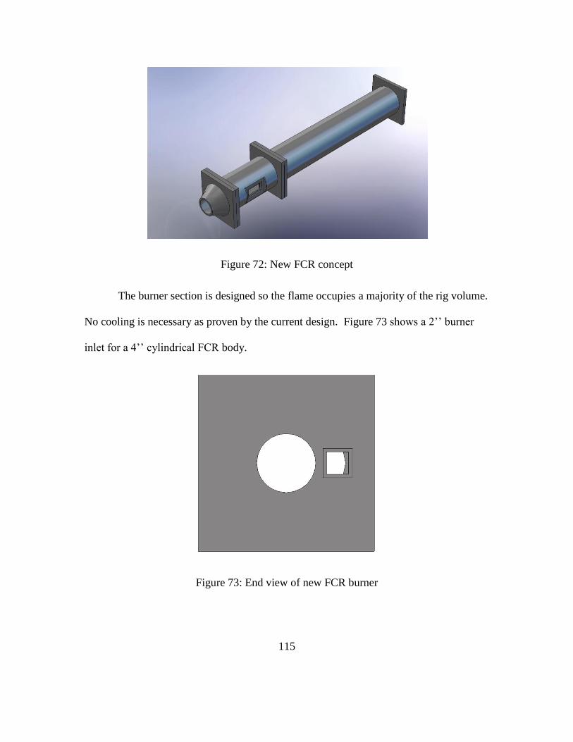
115

Figure 72: New FCR concept

The burner section is designed so the flame occupies a majority of the rig volume.

No cooling is necessary as proven by the current design. Figure 73 shows a 2‘‘ burner

inlet for a 4‘‘ cylindrical FCR body.

Figure 73: End view of new FCR burner

116

A custom glass window allows laser access from the test section wall out 3/4‘‘ in

the radial direction. The burner section is long enough to allow complete combustion of

the fuel/air mixture. A one-piece design using 4‘‘ schedule 40 pipe minimizes the cost,

complexity, and number of seams where undesired air can enter. The square end caps are

welded to the circular body, again preventing air from entering the body.

The test section (Figure 74) is modular, allowing different coolant hole

configurations, but not different curvature radii.

Figure 74: New test section concept

The simplicity of design makes up for this shortfall by allowing completely new

FCR assemblies for a fraction of the cost and effort of the previous design. At each end

of the test section is a mounting plate designed to attach the test section to the other

sections, while preventing air from entering the body of the rig. A high temperature

gasket should be in place between each section. The coolant hole is drilled directly into

the single wall of the test section and coolant enters a plenum attached to the outside of

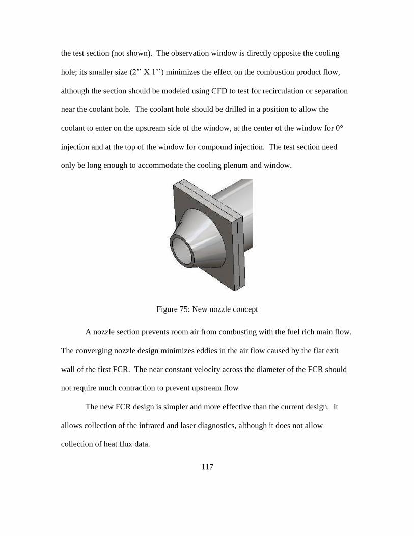
117

the test section (not shown). The observation window is directly opposite the cooling

hole; its smaller size (2‘‘ X 1‘‘) minimizes the effect on the combustion product flow,

although the section should be modeled using CFD to test for recirculation or separation

near the coolant hole. The coolant hole should be drilled in a position to allow the

coolant to enter on the upstream side of the window, at the center of the window for 0°

injection and at the top of the window for compound injection. The test section need

only be long enough to accommodate the cooling plenum and window.

Figure 75: New nozzle concept

A nozzle section prevents room air from combusting with the fuel rich main flow.

The converging nozzle design minimizes eddies in the air flow caused by the flat exit

wall of the first FCR. The near constant velocity across the diameter of the FCR should

not require much contraction to prevent upstream flow

The new FCR design is simpler and more effective than the current design. It

allows collection of the infrared and laser diagnostics, although it does not allow

collection of heat flux data.

118

Appendix A. MKS Type 247 Mass Flow Controller Control Panel Settings

The MKS Type 247D Four-Channel Readout instructions contain all the

necessary information to setup and operate the panel(30). This appendix is included to

show the settings used for the MFCs and gasses used by the FCR. The type 247 was

operated using manual flow control, although the panel is capable of being controlled via

LabVIEW®.

*SCF GF GCF

where SCF is the Scaling Control Factor, GF is the Gauge Factor, and GCF is the Gas

Correction Factor.

Table 6: MFC control panel settings

MFC Size Cal Gas GF Gas GCF SCF

50 SLPM N2 50 C3H8 0.36 18

50 SLPM air 50 zero air 1.00 50

20 SLPM N2 200 C2H4 0.50 100

5 SLPM H2 50 C3H8 0.36 18

100 sccm Xe 100 C3H8 0.27* 27

*The GCF for the Xenon cal gas is 1.32, so the GCF for this MFC is 3 8 0.36

1.32

C H

Xe

GCF

GCF .

For the other MFCs, the GCF of the cal gas is 1.0, so the GCF of the test gas is the GCF.

119

Appendix B. LabVIEW® Procedures

Figure 76: LabVIEW® VI for FCR

a. Open Film Cooling Final_1.VI in the film cooling folder on the control computer

desktop.

b. Start the interface using the ―run‖ button at the top of the program.

c. Select the file location and name

d. Set the Fuel Mass Flow to the max mass flow rate for the burner propane and Phi

to 1.5. Observe the air req’d value for test conditions using the max fuel flow and

φ=1.5.

e. Set the hole diameter and test section area.

120

f. Open Sec Air Valve. Adjust the Secondary Flow Setpoint to the starting condition

(0.25 kg/min). Confirm Secondary Flow has reached the setpoint and settled.

g. After adjusting MFC panel settings to starting conditions, open Zero Air, Coolant,

Ethylene, and Propane Solenoid Valves.

h. After starting gas flow on MFC panel, press the igniter to start wait briefly and

press again to stop the igniter. If the burner fails to start verify gas flows and

settings then attempt again.

i. Once the burner has started and the ethylene and zero air flow is shut off on the

MFC, close the Zero Air and Ethylene Solenoid Valves.

j. Increase the main burner Propane flow to 15 SLPM and then increase the Sec

Flow Setpoint to 0.33 kg/m in 0.02 kg/m increments. Increase the main burner

propane again to the max flow, and then increase the Sec Flow Setpoint to the air

req’d value in 0.02 kg/min increments.

k. Change the coolant flow rate on the MFC panel to the desired blowing ratio

setting and input the value into the Coolant box. Observe the Blowing Ratio

display at the desired value.

l. After the water temperature has stopped increasing (less than 2°C increase over

10 minutes), start IR camera data collection and press the Start Measurement File

2 Write button.

m. Adjust the Phi value to calculate new air flow settings as required. Input new air

flow values into the Sec Flow Setpoint box. Allow to settle.

121

n. Test blowing ratios (0.5, 0.75, 1.00, 1.25, and 1.50) are constantly displayed.

Change the MFC panel and update the Coolant box as required. Other blowing

ratio settings must be hard coded into the program.

o. When the test is complete, turn off gas flow on the MFC panel. Close the

Propane and Coolant Solenoid valves. Burner air flow may be used to cool the

FCR.

p. When airflow in no longer required, change the Sec Flow Setpoint to 0.00 and

close the Sec Air Valve.

q. When all testing is complete, or when a new data file is desired, press the Quit

Program button and close the program.

122

Appendix C. IR Camera Operation

Figure 77: ThermaCam Researcher interface

This appendix is intended to describe the specific setting and procedures used to operate

the IR camera for the FCR. More detailed information for the camera and software is

given in the camera and software user manuals(31)(32).

a. Place the camera opposite the FCR window and record the distance between the

camera and the test section wall at the coolant hole. Ensure the ZnSe window is

installed on the FCR.

b. Connect the AC power cord and firewire cable to the camera. The firewire cable

should be connected to the computer with the Thermacam Researcher software

and the power cord to an AC power outlet.

c. Turn the camera and computer on. Remove the lens cap.

123

d. Start the Thermacam Researcher software. Connect to the camera by selecting

CameraConnect. View the camera image in the main window.

e. If no image is observed press the auto adjust scale button. If no image is

observed select the Cam tab in the Thermacam Firewire window. Verify the

measurement range is set to (-40-120°C) or (0-500°C). If necessary troubleshoot

further using the camera manual.

f. Adjust the image focus in the Cam tab of the Thermacam Firewire window.

Further refinement of the focus is possible using the focus ring on the camera.

g. Remove camera while heating the FCR.

h. Once the FCR has reached steady-state conditions, place the camera opposite the

FCR.

i. In the Cam tab of the Thermacam Firewire window change the measurement

range to (300-2000°C).

j. Select ImageSettings to bring up the camera settings. In the Object Parameter

tab input the desired settings. The settings used for this research are shown

below:

Table 7: ThermaCam Researcher settings

Object

emissivity 0.95

distance 0.4 m

reflected temperature

350 °K

External Optics

124

temperature 350 °K

transmissivity 0.70

Atmosphere

temperature 350°K

humidity 0.20

**These settings were used to get a rough absolute temperature. A thermocouple at the

surface should be used to calibrate the temperature measurements.

k. Select RecordingConditions to set the test data collection parameters. Press the

Image Directory button to set the image location. Create a new folder for each

test. Set the recording parameters in the table below.

Table 8: Data collection settings

Start Tool Button/F5

Record At highest speed

Stop After time duration (0,0,10)

External trig source none

File Format Images in multiple files

auto name base set to test name

l. When ready to start data collection press F5 or the Start button.

m. Output the image files to MATLAB® by selecting RecordingCopy Selection.

output directory: choose, Output name: same as source, Output format:

MATLAB.

125

The result of this operation is 300 MATLAB® files each with a 640 by 480 array

of temperature data. The code in Appendix D processes the image files.

126

Appendix D. MATLAB® Code

%% Curved Image Expansion Tool %%%%%%%%%%%%%%%%%%%%%%%%%%%%%%%%%%%%%%%%%%%%%%%%%%%%%%%%%%%%%%%%%%%%%%%

%%%% % Created by Mike Miller - miller.462@wright.edu - (937)450-0488

% %%%%%%%%%%%%%%%%%%%%%%%%%%%%%%%%%%%%%%%%%%%%%%%%%%%%%%%%%%%%%%%%%%%%%%%

%%%% % This program opens multiple images saved as .mat files, averages the % images together, "unfolds" the curved portion of the new image, and

crops % the new image to a user-defined size. % % The variable inputs are: % - The radius of the curve (r) % - The height of each pixel (h) % - The multiplication factor for the arc ratios (q) % - The coolant hole diameter (chd) % The prompted user inputs are: % - The location of the bottom of the curved test section % - 2 corner points of the area to be cropped % % NOTE: When selecting the bottom of the test section, you MUST CLICK

ABOVE % 100 pixels from the bottom of the image for a 4-inch curve. %%%%%%%%%%%%%%%%%%%%%%%%%%%%%%%%%%%%%%%%%%%%%%%%%%%%%%%%%%%%%%%%%%%%%%%

%%%%

%% Close & Clear all close all clear all clc %% Variable Inputs %Radius of test section r=4; %The physical height(y-dimension) of each pixel (inches/pixel) h=(1/95); %q is the multiplication factor of the arcratios(higher q means the

arcratio is more accurate) q=10; %Coolant hole diameter(inches) chd=.07; %% Open File dir1=pwd; [A,pathname]=uigetfile('*.mat','Select .mat Files to

Evaluate','MultiSelect','on'); cd(pathname); list=strvcat(A); %#ok<VCAT> [t,u]=size(list); for i=1:t uiopen(list(i,:),1); drawnow;

127

commandwindow; %Find and Remove the file extension from the filename n=length(list(1,:)); for j=1:n X=uint8(list(i,j)); periodlocation=0; if (X==46) periodlocation=j; break end end m=periodlocation-1; Alist=list(1:t,1:m); end %Create variable names for each matrix and put them in a column vector B=0;B1=0;B2=0;B3=0;B4=0;B5=0;B6=0;B7=0;B8=0;B9=0; B10=0;B11=0;B12=0;B13=0;B14=0;B15=0;B16=0;B17=0;B18=0;B19=0; B20=0;B21=0;B22=0;B23=0;B24=0;B25=0;B26=0;B27=0;B28=0;B29=0; B30=0;B31=0;B32=0;B33=0;B34=0;B35=0;B36=0;B37=0;B38=0;B39=0; B40=0;B41=0;B42=0;B43=0;B44=0;B45=0;B46=0;B47=0;B48=0;B49=0; B50=0;B51=0;B52=0;B53=0;B54=0;B55=0;B56=0;B57=0;B58=0;B59=0; B60=0;B61=0;B62=0;B63=0;B64=0;B65=0;B66=0;B67=0;B68=0;B69=0; B70=0;B71=0;B72=0;B73=0;B74=0;B75=0;B76=0;B77=0;B78=0;B79=0; B80=0;B81=0;B82=0;B83=0;B84=0;B85=0;B86=0;B87=0;B88=0;B89=0; B90=0;B91=0;B92=0;B93=0;B94=0;B95=0;B96=0;B97=0;B98=0;B99=0; B100=0; Blist=zeros(t,4); for i=1:t newB= genvarname('B',who); eval([newB ' = eval(Alist(i,:))']); Blist(i,:)=newB(:,:); Clist=char(Blist); end %Concatenate all matrices into a 3D array and average them together P=eval(Clist(1,:)); for i=2:t Pnew=cat(3,P,eval(Clist(i,:))); P=Pnew; end E=mean(P,3); %Flip matrix E and create contour plot C=flipud(E); figure('Name','Average','NumberTitle','off'); contourf(C,'linestyle','none'); colormap(jet), colorbar; %% User Input disp('Click on the bottom of the test section'); [x,y]=ginput(1); close disp('Please Wait...'); %% Calculations %Total pixels in y-direction for entire test section ypixels=480-round(y);

128

%Calculate the arc length and arc ratio of each section count=0; D=[ypixels,1]; for i=0:ypixels-1 %The distance(inches) from the bottom of the curve to the bottom of the

current pixel ybot=i*h; %The distance(inches) from the bottom of the curve to the top of the

current pixel ytop=ybot+h; %"b" is the distance from the top of the curve to the bottom of the

current pixel b=r-ybot; %"a" is the distance from the top of the curve to the top of the

current pixel a=r-ytop; %x-dimension of the top of the pixel with respect to "a" and "r" xtop=inline('sqrt((2*r*a)-(a^2))'); %x-dimension of the bottom of the pixel with respect to "b" and "r" xbot=inline('sqrt((2*r*b)-(b^2))'); %x-dimension of the arclength xarc=inline('xbot-xtop'); %Arc length of the pixel arclength=inline('(pi*r*asin(sqrt(xarc^2+h^2)/(2*r)))/(pi/2)'); %Ratio of arclength to y-dimension of the pixel arcratio=arclength(h,r,xarc(xbot(b,r),xtop(a,r)))/h; arcratio10=round(q*arcratio); count=count+arcratio10; %Column vector of the arcratios of each pixel in the selected section D(1+i,:)=arcratio10; end %% Build New Matrix newrows=count+round(y)*q; %Build the bottom section of the new matrix up to the input y-value M=ones(newrows,640); newcount=0; j=1; for i=1:round(y) qstart=newcount+1; for l=1:640 M(qstart:newcount+q,l)=C(j,l); end j=j+1; newcount=newcount+q; end %Build the rest of the matrix using the adjusted values newcount=round(y)*q; p=0; for i=round(y)+1:480 p=p+1; k=D(p); kstart=newcount+1; for l=1:640

129

M(kstart:newcount+k,l)=C(i,l); end newcount=newcount+k; end %PLOT THE ADJUSTED FIGURE figure('Name','Adjusted Average','NumberTitle','off'); contourf(M,'linestyle','none'); colormap(jet), colorbar; xlabel('Coolant Hole Diameters','fontsize',9,'fontweight','b'); ylabel('Coolant Hole Diameters','fontsize',9,'fontweight','b'); %SET FIGURE AXES TO HOLE DIAMETERS %Coolant hole diameter in inches/(pixel height) xdiam=chd/h; xlimit=640/xdiam; set(gca, 'XTick', 0:xdiam:640); set(gca, 'XTickLabel', (0:1:xlimit),'fontsize',7); ydiam=xdiam*q; ylimit=newrows/ydiam; set(gca, 'YTick', 0:ydiam:newrows); set(gca, 'YTickLabel', (0:1:ylimit),'fontsize',7); %% Crop Image %Input corner points of area to be cropped disp('Click on top left corner of crop area'); [x1,y2]=ginput(1); disp('Click on bottom right corner of crop area'); [x2,y1]=ginput(1); Y1=round(y1); Y2=round(y2); X1=round(x1); X2=round(x2); dx=X2-X1; dy=Y2-Y1; Mcrop=ones(dy,dx); j=Y1; for i=1:dy k=X1; for l=1:dx Mcrop(i,l)=M(j,k); k=k+1; end j=j+1; end %Plot the cropped image figure('Name','Cropped Average','NumberTitle','off'); contourf(Mcrop,'linestyle','none'); colormap(jet), colorbar; xlabel('Coolant Hole Diameters','fontsize',9,'fontweight','b'); ylabel('Coolant Hole Diameters','fontsize',9,'fontweight','b'); %SET FIGURE AXES TO HOLE DIAMETERS %Coolant hole diameter in inches/(pixel height) xdiam2=chd/h; xlimit2=dx/xdiam2; set(gca, 'XTick', 0:xdiam2:dx);

130

set(gca, 'XTickLabel', (0:1:xlimit2),'fontsize',7); ydiam2=xdiam2*q; ylimit2=dy/ydiam2; set(gca, 'YTick', 0:ydiam2:dy); set(gca, 'YTickLabel', (0:1:ylimit2),'fontsize',7); %% Return to Original Directory cd(dir1); %% Re-Run Program? restart=input('Press 1 to restart program, 2 to quit. '); if restart==1 CIET_multiple_images.m else break end

131

Bibliography

1. Holt, James B and Monk, Timothy S. Propellant mass Fraction Calculation

Methodology For Launch Vehicles and Application to Ares Vehicles. Huntsville,

AL : s.n.

2. McCall, Jonathan Floyd. Discrete Film Cooling in a Rocket with Curved Walls. ENY,

Air Force Institute of Technology. 2009.

3. Humble, Ronald W., Henry, Gary N. and Larson, Wiley J. Space Propulsion Analysis

and Design. First Edition-Revised. New York : The McGraw-Hill Companies, Inc.,

1995. p. 524. ISBN 0-07-031320-2.

4. Wertz, James R. and Larson, Wiley J., [ed.]. Space Mission Analysis and Design. 3rd.

Hawthorne : Microcosm Press, 2008.

5. Rutledge, James L. Pulsed Film Cooling on a Turbine Edge Leading Edge. Air Force

Institute of Technology. 2009. Doctoral Dissertation.

6. Rannie, W. D. A Simplified Theory of Porous Wall Cooling. Jet Propulsion Laboratory,

California Institute of Technology. 1947. ORDCIT Progress Report No. 4-50.

7. May, Lee and Burkehardt, W.M. Transpiration Cooled Throat for Hydrogen Cooled

Rocket Engines. Aerojet Propulsion Division. Sacramento, CA : s.n., 1991. NASA

Contract NAS 8-36952.

8. Chen, Fu-Jung. Effects of Blowing Ratios on Heat Transfer to the Throat Region of a

Porous-Walled Nozzle. Air Force Institute of Technology. 1995. Masters Thesis.

9. Lenertz, Joseph L. Effects of Blowing Ratio on Heat Transferto the Throat Region of a

Porous-Walled Nozzle. Air Force Institute of Technology. 1994.

10. Landis, Jay A. Numerical Study of a Transpiration Cooled Rocket Nozzle. Air Force

Institute of Technology. 1995. Masters Thesis.

11. Huzel, Dieter K and Huang, David H. Modern Engineering for Design of Liquid-

Propellant Rocket Engines. 3rd. Washington D.C. : The American Institute of

Aeronautics and Astronautics, Inc., 1992. p. 101.

132

12. Spalding, D. B. Convectice Mass Transfer. New York : McGraw-Hill Book

Company, Inc, 1963. p. 38.

13. The Turbulent Boundary Layer on a Porous Plate: Experimental Skin Friction With

Variable Injection and Suction. Simpson, Roger L., Moffat, R. J. and Kays, W. M.

London : s.n., 1969, International Journal of Heat and Mass Transfer, Vol. 12, pp.

771-789.

14. Kays, W. M. and Crawford, M. E. Convective Heat and Mass Transfer. New York :

McGraw-Hill Book Company, 1980.

15. Hartnett, James P. and Irvine, Thomas F., [ed.]. Advances in Heat Transfer. New

York : Academic Press, 1965. Vol. 2.

16. Keener, David N. Investigation of Boundary Layer and Performance Effects of

Transpiration Cooling Through a Porous Plate in a Rocket Nozzle. Air Force

Institute of Technology. 1994. Masters Thesis.

17. Anderson, Wesly S. Design, Construction, and Validation of the AFIT Small-Scale

Combustion Facility and Sectional Model of the Ultra-Compact Combustor. AFIT.

2007. Masters Thesis.

18. Koether, Stephen J. Validation of the AFIT Small-Scale Combustion Facility and OH

Laser-Induced Florescence of an Atmospheric Laminar Premixed Flame. AFIT.

2007. Masters Thesis.

19. Hankins, Terry B. Laser Diagnostic System Validation and Ultra-Compact

Combustor Characterization. AFIT. 2008. Masters Thesis.

20. Lakusta, Patrick J. Laser-Induced Fluorescence and Performance Analysis of the

Ultra-Compact Combustor. AFIT. 2008. Masters Thesis.

21. Drenth, Aaron C. Laser-Induced Fluorescence and Synthetic Jet Fuel Analysis in the

Ultra Compact Combustor. AFIT. 2009. Masters Thesis.

22. Thomas, Levi M. Flow Measurements Using Particle Image Velocimetry in the Ultra

Compact Combustor. AFIT. 2009. Masters Thesis.

23. Bohnert, Alex M. Thermal Characterization of a Hall Effect Thruster. AFIT. 2008.

Masters Thesis.

133

24. Kim, Ted T. Thermo-Mechanical Characterization of Silicon Carbide-Silicon

Carbide Composites at Elevated Temperatures Using a Unique Combustion Facility.

AFIT. 2009. Doctoral Dissertation.

25. Dittman, Eric R. Design, Build, and Construction of a Small Scale Combustion

Chamber Testing Facility. AFIT. 2006. Masters Thesis.

26. Turns, Stephen R. An Introduction to Combustion. 2nd. Boston : McGraw Hill, 2000.

27. Sutton, George P. and Biblarz, Oscar. Rocket Propulsion Elements. New York : John

Wiley and Sons, Inc., 2001.

28. General Thermocouple Specifications. Omega.com. [Online] Omega. [Cited: 02 15,

2010.]

http://www.omega.com/toc_asp/frameset.html?book=Temperature&file=TC_GEN_S

PECS_REF.

29. FLIR P640 Infrared Camera Datasheet. Portland, OR : FLIR Systems Co. LTD.

30. Approximate Temperature of Steel by Color. Muggy Weld. [Online] [Cited: January

29, 2010.] http://www.muggyweld.com/color.html.

31. MKS Type 247D Four-Channel Readout User Manual. Andover, MA : MKS

Instruments, 07 1997. Rev A.

32. ThermaCAM Researcher User's Manual. s.l. : FLIR Systems, 2006.

33. FLIR 600 Series User's Manual. s.l. : FLIR Systems, 2009.

34. Von Karman, Theodore and Edson, Lee. The Wind and Beyond. Boston : Little,

Brown, and Company, 1967. .

134

Vita

Major Sincock is a 1999 graduate of the United States Air Force Academy where

he studied Engineering Mechanics. His first assignment was to Malmstrom AFB,

Montana, where he was an operational ICBM crew commander and instructor. Major

Sincock was a member of the best ICBM operations team in Air Force Space Command

during the 2002 Guardian Challenge competition.

As an Air Force engineer, Major Sincock led the ground station development for

the Space Radar Integrated Program Office, working closely with the National

Reconnaissance Office and the National Geo-spatial Intelligence Agency. He was then

selected to join the Navy Mobile User Object System Program Office (PMW-146) as the

lead for EELV launch integration. During this time he worked closely with the Air Force

EELV team, the Navy, and the satellite and launch vehicle contractors to coordinate the

first ever launch of a major Navy satellite using an Air Force launch vehicle.

After graduation in March 2010, Major Sincock reports to the Space and Missile

Propulsion Division of the Air Force Research Laboratory at Edwards AFB, California,

continuing his career-long focus on space and missile operations and development for the

Air Force.

REPORT DOCUMENTATION PAGE Form Approved OMB No. 074-0188

The public reporting burden for this collection of information is estimated to average 1 hour per response, including the time for reviewing instructions, searching existing data sources, gathering and maintaining the data needed, and completing and reviewing the collection of information. Send comments regarding this burden estimate or any other aspect of the collection of information, including suggestions for reducing this burden to Department of Defense, Washington Headquarters Services, Directorate for Information Operations and Reports (0704-0188), 1215 Jefferson Davis Highway, Suite 1204, Arlington, VA 22202-4302. Respondents should be aware that notwithstanding any other provision of law, no person shall be subject to an penalty for failing to comply with a collection of information if it does not display a currently valid OMB control number.

PLEASE DO NOT RETURN YOUR FORM TO THE ABOVE ADDRESS.

1. REPORT DATE (DD-MM-YYYY)

25-03-2010 2. REPORT TYPE

Master’s Thesis 3. DATES COVERED (From – To)

Sep 2008 – Mar 2010 4. TITLE AND SUBTITLE

Design Of A Film Cooling Experiment For Rocket Engines

5a. CONTRACT NUMBER

5b. GRANT NUMBER

5c. PROGRAM ELEMENT NUMBER

6. AUTHOR(S)

Sincock, Andrew, L., Major, USAF

5d. PROJECT NUMBER

5e. TASK NUMBER

5f. WORK UNIT NUMBER

7. PERFORMING ORGANIZATION NAMES(S) AND ADDRESS(S)

Air Force Institute of Technology

Graduate School of Engineering and Management (AFIT/ENY)

2950 Hobson Way, Building 640

WPAFB OH 45433-8865

8. PERFORMING ORGANIZATION REPORT NUMBER

AFIT/GAE/ENY/10-M23

9. SPONSORING/MONITORING AGENCY NAME(S) AND ADDRESS(ES)

Michael Huggins

Air Force Research Laboratory

Propulsion Directorate

4 Draco Drive

Edwards AFB, CA 93524

10. SPONSOR/MONITOR’S ACRONYM(S)

AFRL 11. SPONSOR/MONITOR’S REPORT NUMBER(S)

12. DISTRIBUTION/AVAILABILITY STATEMENT

APPROVED FOR PUBLIC RELEASE; DISTRIBUTION UNLIMITED.

13. SUPPLEMENTARY NOTES

14. ABSTRACT

The Film Cooling Rig (FCR) is a new test rig at the Air Force Institute of Technology (AFIT) to study film cooling

for rocket engine applications. The original researcher designed, built, and then utilized the FCR to study radial

curvature effects on film cooling for a non-combustion environment. This effort modified the FCR by adding

propane-air combustion. Modular stainless steel test sections were produced to allow study of various curvatures and

coolant injection angles. A pre-mixed burner was designed and built to deliver main flow mass flow rates necessary

to produce blowing ratios as low as 0.5. A water cooling system was designed for the entire FCR, but only

implemented for the curved test sections. Instrumentation in this system allows calculation of the average heat flux to

the test section. Once the necessary FCR and lab modifications were accomplished, the operating range of the FCR

was developed and tested using infrared thermography. Surface temperature measurements near the cooling hole

showed no cooling effect for 13 major test configurations, and many more minor variations. The lack of cooling was

caused by inadequate spreading of the burner flow to the test section wall. Without the necessary main flow

momentum across the test section wall, the coolant flow did not turn and adhere to the wall. Instead, it jetted into the

main flow without cooling the wall as expected. Recommendations included modifications to the existing rig to

correct the main flow issue, along with a completely new FCR design incorporating the lessons learned from this

research to produce a simpler, more effective rig. The new design allows the laser and infrared diagnostics of the first

rig without the manufacturing complications that hindered testing in the first FCR. 15. SUBJECT TERMS

Combustion, Rocket, Film, Cooling, Transpiration, Infrared

16. SECURITY CLASSIFICATION OF:

17. LIMITATION OF ABSTRACT

UU

18. NUMBER OF PAGES

154

19a. NAME OF RESPONSIBLE PERSON

Richard Branam, Lt Col, USAF a. REPORT

U

b. ABSTRACT

U

c. THIS PAGE

U

19b. TELEPHONE NUMBER (Include area code)

(937)255-6565, ext 6485

Standard Form 298 (Rev. 8-98) Prescribed by ANSI Std. Z39-18