Design methodology accounting for the effects of … · 1 Design methodology accounting for the...
54
1 Design methodology accounting for the effects of porous medium heterogeneity on hydraulic residence time and biodegradation in horizontal subsurface flow constructed wetlands A. Brovelli 1 , O. Carranza-Diaz, L. Rossi, D.A. Barry Laboratoire de technologie écologique, Institut d’ingénierie de l’environnement, Ecole Poly- technique Fédérale de Lausanne (EPFL), Station No. 2, CH-1015 Lausanne, Switzerland E-mails: [email protected] , [email protected] , [email protected] , [email protected] Telephone: +41 (21) 693-5919, +41 (21) 693-5576 Facsimile: +41 (21) 693-8035 Re-submitted to Ecological Engineering, 20 April 2010 1 Author to whom all correspondence should be addressed
-
Upload
truongthuan -
Category
Documents
-
view
218 -
download
0
Transcript of Design methodology accounting for the effects of … · 1 Design methodology accounting for the...

1
Design methodology accounting for the effects of porous medium
heterogeneity on hydraulic residence time and biodegradation in
horizontal subsurface flow constructed wetlands
A. Brovelli1, O. Carranza-Diaz, L. Rossi, D.A. Barry
Laboratoire de technologie écologique, Institut d’ingénierie de l’environnement, Ecole Poly-
technique Fédérale de Lausanne (EPFL), Station No. 2, CH-1015 Lausanne, Switzerland
E-mails: [email protected], [email protected], [email protected],
Telephone: +41 (21) 693-5919, +41 (21) 693-5576
Facsimile: +41 (21) 693-8035
Re-submitted to Ecological Engineering, 20 April 2010
1 Author to whom all correspondence should be addressed

2
ABSTRACT
Horizontal flow constructed wetlands are engineered systems capable of eliminating a
wide range of pollutants from the aquatic environment. Nevertheless, poor hydrodynamic
behavior is commonly found resulting in preferential pathways and variations in both (i)
the hydraulic residence time distribution (HRTD) and, consequently, (ii) the wetland’s
treatment efficiency. The aim of this work was to outline a methodology for wetland design
that accounts for the effect of heterogeneous hydraulic properties of the porous substrate
on the HRTD and treatment efficiency. Biodegradation of benzene was used to illustrate the
influence of hydraulic conductivity heterogeneity on wetland efficiency. Random, spatially
correlated hydraulic conductivity fields following a log-normal distribution were generated
and then introduced in a subsurface flow numerical model. The results showed that the
variance of the distribution and the correlation length in the longitudinal direction are key
indicators of the extent of heterogeneity. A reduction of the mean hydraulic residence time
was observed as the extent of heterogeneity increased, while the HRTD became broader
with increased skewness. At the same time, substrate heterogeneity induced preferential
flow paths within the wetland bed resulting in variations of the benzene treatment efficien-
cy. Further to this it was observed that the distribution of biomass within the porous bed
became heterogeneous, rising questions on the representativeness of sampling. It was con-
cluded that traditional methods for wetland design based on assumptions such as a homo-
geneous porous medium and plug flow are not reliable. The alternative design methodolo-
gy presented here is based on the incorporation of heterogeneity directly during the design
phase. The same methodology can also be used to optimize existing systems, where the
HRTD has been characterized with tracer experiments.

3
KEYWORDS
Hydraulic residence time distribution, sand filter, treatment efficiency, benzene, reactive
transport modeling, wastewater treatment, optimization.
1. Introduction
The use of subsurface flow constructed wetlands and sand filters as wastewater treatment
technology has been steadily increasing over the last two decades (Vymazal and Kröpfe-
lová, 2008). These systems are appealing because they require only a moderate energy in-
put and are low-maintenance. Wastewater flows through a porous substrate where biolog-
ical and inorganic reactions transform and remove the contaminants (Kadlec and Wallace,
2009). Depending on the flow direction, subsurface flow constructed wetlands (CWs) are
further classified as horizontal (HSCWs) or vertical flow. In HSCWs the porous substrate is
water-saturated except for the uppermost layer. Instead, in vertical flow constructed wet-
lands the bed is variably saturated.
HSCWs have been successfully employed to remove classical contaminants from wastewa-
ters, such as the organic load, nutrients (mainly nitrogen and phosphorous) and pathogens
(Caselles-Osorio and García, 2006; Akratos and Tsihrintzis, 2007; Vymazal, 2007; Reinoso
et al., 2008; Stott et al., 2008; Kadlec, 2009). Recently, several studies have reported the use
of constructed wetlands for removing emerging pollutants, such as pharmaceuticals and
personal care products, hydrocarbons as well as other organic compounds (Wallace, 2001;
Matamoros and Bayona, 2006; Matamoros et al., 2007a, 2008; Lin et al., 2008). Overall,

4
these works observed that this technology is potentially suitable to degrade even recalci-
trant contaminants if present at low concentrations. However, the conditions for the trans-
formation reactions are often sub-optimal and high degradation rates are seldom achieved,
even for traditional contaminants (Hench et al., 2003; Kadlec, 2003). The low removal effi-
ciency has been attributed to several reasons, including incomplete understanding of the
purification mechanisms (Haberl et al., 2003; Imfeld et al., 2009) and the non-
homogeneous distribution of the porous substrate. This latter leads to poor hydrodynamic
behavior of the system, which results from a broad distribution of the hydraulic residence
time (HRT) and associated preferential flow paths (Suliman et al., 2005; Knowles et al.,
2008; Mena et al., 2008; Ascuntar-Rios et al., 2009). This aspect appears to be critical in
particular for HSCWs where the treatment efficiency decreases significantly compared with
vertical systems (Matamoros et al., 2007b, 2008).
In order to understand the hydrodynamics of constructed wetlands, characterization of the
subsurface flow paths using tracer experiments is useful (King et al., 1997; Grismer et al.,
2001; Muñoz et al., 2006). For an ideal, homogeneous porous medium, symmetric Gaussian
breakthrough curves (BTCs) are produced (Kadlec and Wallace, 2009). However, in prac-
tice, multiple peaks, spreading and asymmetric BTCs are frequently observed indicating a
complex hydrodynamic flow field (Barry, 1990; Bajracharya and Barry, 1997; Kamra et al.,
2001). Preferential flow paths in the subsurface, for instance, can lead to considerable va-
riability in the HRT. The heterogeneity of the filtering media is due to multiple factors, in-
cluding (i) changes in porosity and (ii) grain size distribution, (iii) presence of plant roots
and rhizomes, (iv) biological, physical and chemical clogging and (v) variations induced by
different packing and compaction of the bed (Persson et al., 1999; Rash and Liehr, 1999;

5
García et al., 2004; Małoszewski et al., 2006; Kjellin et al., 2007; Brovelli et al., 2009; Leve-
renz et al., 2009).
Tracer experiments to study the factors controlling the porous medium heterogeneity in
HFCWs were conducted by Suliman et al. (2005). They reported that hydrodynamics in
HSCWs becomes more complex as the scale of the system increases, behavior that is also
found in natural aquifers (Gelhar et al., 1992). Suliman et al. (2006a,b) also investigated the
effect of the inlet position on the hydraulic performance of HSCWs, while the effect of the
different filling configurations of the wetland was reported by Suliman et al. (2007). A cor-
relation between the hydraulic residence time distribution (HRTD) and the extent of hete-
rogeneity was observed and it was found that filling the system in vertical sections led to
better hydraulic efficiency. Małoszewski et al. (2006) investigated the variability of hydrau-
lic parameters in gravel cells. The hydraulic conductivity was found to vary in the vertical
direction, resulting in heterogeneous transport parameters and leading to an uneven flow
pattern and HRT variability. A common finding of these works is that porous medium hete-
rogeneity controls the HRTD and, consequently, the treatment efficiency of subsurface flow
constructed wetlands and sand filters. More specifically, the treatment efficiency of HSCWs
is correlated to the HRT (Chin, 2006; Kadlec and Wallace, 2009). The relationship can be
understood considering that pollutant elimination occurs only if the contact time between
active microbial biomass and contaminated water is sufficiently long to promote the bio-
logical and abiotic reactions able to remove the contaminant from the water.
If treatment efficiency is a function of the HRT alone, it follows that the optimal efficiency is
achieved when the HRTD is narrow, a situation that is approached most closely in a homo-

6
geneous medium. However, this rarely occurs thereby resulting in suboptimal treatment
efficiency (Persson et al., 1999; Chazarenk et al., 2003; Jenkins and Greenway, 2005). Cor-
rect sizing of HSCWs during the design phase is therefore of paramount importance to
guarantee high removal rates and good functioning in a wide range of operational condi-
tions. To date, however, dimensioning is still mostly based on empirical rules, such as the
surface-area-per-equivalent-person criterion. A notable exception is the P-k-C* model of
Kadlec and Wallace (2009). Their approach is derived from the tank-in-series model, and it
is particularly appealing because combines simplicity with the ability to incorporate the
stochastic variability of the treatment efficiency due, among other reasons, to variations in
retention time. HSCWs are becoming increasingly used in more critical applications and to
remove emerging contaminants (i.e., organic compounds). As a consequence, traditional
design methods may not be suitable to guarantee high water quality levels and new and
more robust design tools are sought (Kadlec, 1997). While the connection between the he-
terogeneous distribution of the hydraulic conductivity, HRTD and removal efficiency is now
widely recognized (Marsili-Libelli and Checchi, 2005; Suliman et al., 2005; Wörman and
Kronnäs, 2005), it is not known how the design process can be improved to take it into ac-
count, and how the negative or positive effects of heterogeneity in working systems can be
controlled. Numerical models have been extensively used in numerous applications in the
field of the environmental sciences and engineering (such as hydrogeology, soil science,
petroleum engineering, etc.) to analyze the effect of heterogeneity on solute transport and
biogeochemical reactions. The chemical, physical and biological processes responsible for
wastewater purification in CWs are the same as those that produce, for example, organic
matter and nutrient transformations in soils and aquifers. Therefore, the same concepts

7
and the same numerical tools developed in these fields can be applied to study CWs. De-
spite this similarity and the availability of numerous commercial and open-source numeri-
cal tools (http://water.usgs.gov/software/lists/groundwater/, http://www.pmwin.net/,
http://www.goldsim.com/Content.asp?PageID=26, http://www.pht3d.org/, amongst many
others), modeling of wastewater purification in CWs is still limited to the extent that de-
tailed model-based design is far from commonplace. Some emerging models are now avail-
able in the literature and have shown that they can be successfully applied to full-scale CWs
(e.g., Dittmer et al., 2005; Mayo and Bigambo 2005; McGechan et al., 2005; Langergraber,
2007, 2008; Langergraber et al., 2009a; Toscano et al., 2009; Giraldi et al., 2010). The con-
cept and processes linked to heterogeneity are however not addressed in these approach-
es. The aim of this work is therefore to analyze the relationship between amount of hetero-
geneity, HRTD and removal efficiency, and to develop a suitable methodology to incorpo-
rate heterogeneity into the design phase. In particular, er to show that process-based de-
sign of CWs can be effectively conducted using readily available numerical tools, the strate-
gy presented in the following makes use of a combination of techniques and numerical
models developed in other fields that can be readily applied to this type of wastewater
treatment system.
2. Methodology
The methodology proposed in this work to study the effect of heterogeneity and to improve
the design of constructed wetlands and sand filters combines two concepts. The first is that
of the target HRT (or THRT), which is the shortest HRT such that a system will degrade a
given contaminant below a target concentration. In real systems treating wastewaters with

8
a large spectrum of pollutants, the THRT is controlled by the most recalcitrant and toxic
contaminant, for which the allowed effluent concentrations are lower. The THRT is linked
to the contaminant degradation rate, which in turn depends on biomass capabilities and on
the environmental conditions of the porous bed (e.g., oxygen availability, temperature,
etc.). The THRT can be estimated from previous experience, and further can be corrobo-
rated and integrated using numerical models able to reproduce the complex biological
transformations occurring in the wetland (Langergraber et al., 2009a). The second concept
concerns the HRTD. The HRTD depends on the physical properties of the wetland, and on
the hydraulic conductivity distribution and the influent rate in particular. Indeed, the me-
thodology described below is based on the assumption that the treatment efficiency is a
function of the HRTD.
While the inflow rate is a design parameter and can be controlled at least to some extent,
the hydraulic conductivity distribution is difficult to know a priori with sufficient detail to
be used in a standard design approach. To overcome this difficulty, the variability in the
hydraulic conductivity distribution is characterized using a numerical stochastic approach.
The underlying assumption is that the hydraulic conductivity distribution is spatially corre-
lated and the resulting field can be represented as a random function, characterized by a
limited number of parameters. This has been recently confirmed in numerous experiments
where it was also shown that the spatial correlation depends on the filling configuration
(Suliman et al., 2007). The methodology proposed to incorporate the effect of heterogenei-
ty is given by the following steps:

9
1. A THRT is defined depending on the most persistent contaminant, or the contaminant
for which the smallest concentration in the discharged water is needed. That is, it is the
smallest HRT for which water quality standards of the effluent from the system would
be satisfied. This parameter can be defined based on past experience (literature data),
small scale experiments and/or mechanistic numerical modeling of the degradation
processes.
2. Numerical simulations are conducted to evaluate the HRTD of a given system (defined
by classical design parameters, such as the loading rate) considering multiple realiza-
tions of the same hydraulic conductivity distribution (i.e., every realization of the hy-
draulic conductivity field has the same statistical properties). At this stage, the system
considered has the largest dimensions that can be allowed in reality, and the goal of the
methodology is to identify if and to what extent they can be reduced to achieve the tar-
get effluent concentration. The hydraulic conductivity distribution depends on the
physical properties of the porous medium (e.g., spatial variations in the grain size dis-
tribution) and on the strategy used to fill the HFCW basin (Suliman et al., 2007). This
latter aspect can however be controlled during construction. How a random hydraulic
conductivity distribution can be generated, and how its parameters are defined will be
discussed in the following.
3. Combining the outcome of the simulations with the THRT, the probability of failure of
the system (PFS) at a given distance from the inlet can be computed. For example, if 10
realizations of the hydraulic conductivity field are used, and at one location in eight
cases the observed mean HRT is larger than the THRT, then the PFS is 0.2. The PFS is a
metric that indicates how likely it is that the target contaminant concentration will be

10
obtained at a certain distance from the inlet. It can be computed for a given system us-
ing the method presented in point 2 above (and discussed in more detail in §2.4).. The
methodology presented here only accounts for the variations in hydraulic residence
time. In reality, however, there is a second important source of uncertainty, that is, sto-
chastic variability of the degradation rates (e.g., Kadlec and Wallace, 2009). While this
aspect was not considered, the method presented in this work can be further extended
to include it, although at the cost of additional complexity.
4. The sizing of the system is based on this information. Ideally, the size will achieve a PFS
of 0, meaning a probability of 100% to achieve a given elimination goal. In other situa-
tions, for example when the loading rate considered is at one extreme end of the ex-
pected range, a larger PFS could be used, in order not to over-dimension the system.
Furthermore, there could be situations where the maximum possible dimensions do
not suffice to guarantee that the target concentration is achieved. In these cases, alter-
native options must be considered (e.g., the loading rate must be reduced to increase
the HRT, a different treatment technology should be employed, discussion with the lo-
cal authorities to accept the predicted efficiency of the system, etc.). This is a classical
procedure in probabilistic environmental risk assessment approaches (Barnett and
O’Hagan, 1997; Rossi et al., 2009).
The same approach can also be used to optimize the performance of working systems.
First, the HRTD is characterized using tracer experiments, and the inflow rate is reduced
consequently to achieve the THRT. The underlying assumption of this procedure is that the
HRT and the flow rate are linearly correlated. This is clearly true in homogeneous condi-
tions since the flow rate can be described using Darcy’s law. In more complex situations,

11
where the flow field is irregular due to heterogeneity, diffusion of solutes into the low con-
ductivity (or stagnant) zones might become important and modify the linear scaling of the
contaminant residence time with the inlet flow rate (or the hydraulic gradient). The validi-
ty of this assumption will be tested in the following.
2.1 Test case set-up
A realistic test-case was developed to illustrate the methodology and analysis of the rela-
tionship between porous medium heterogeneity, HRTD and treatment efficiency. While the
analysis presented in the following is relevant to a specific case, the approach can be ap-
plied to any contaminant undergoing kinetic degradation in the treatment system. Moreo-
ver, in terms of the understanding of the relationship between the heterogeneous hydraulic
conductivity, HRTD and treatment efficiency, the findings are also not restricted to the spe-
cific set-up used here.
A 10-m long and 1-m deep HSCW was considered in all the simulations presented in this
work. Since the goal of our approach is identify the optimal size for the system (in this case
only the dimension along the flow direction will be adjusted), the chosen length represents
the upper length limit. In other words, the optimal length will be selected based on the
analysis that follows, but cannot be longer than 10 m. This upper limit can be in practice
decided depending on the available space or considering economic constraints. For the
sake of simplicity and to keep the computational effort moderate, we only consider a two-
dimensional vertical cross section of the system to be modeled. Preliminary numerical ex-
periments were conducted to evaluate whether heterogeneity in the transverse horizontal
direction affected the HRTD. It was observed that, while it has an effect, it is nearly the

12
same as the influence of the heterogeneity in the vertical direction and for this reason a
two-dimensional cross-section suffices. Nonetheless, a two-dimensional flow system is
known to give different results to a three-dimensional system. For example, Dagan (1989)
has shown for an isotropically (referring to correlation length) log-normally distributed
hydraulic conductivity that the effective hydraulic conductivity is always the corresponding
geometric mean in two-dimensions and is always greater than the geometric mean in three
dimensions, at least for spatially infinite domains. Thus, for such a medium, it is expected
that the HRT is always greater in two dimensions than in three dimensions, other things
being equal. Put another way, the three-dimensional system usually has more degrees of
freedom in terms of flow paths through it, in which case the effective hydraulic conductivi-
ty would normally be expected to be greater than in two-dimensions. For finite domains,
such as that considered below, it has been found that the effective conductivity is expected
to be higher than the geometric mean (Hristopulos, 2003). This result was found in the
numerical results reported below.
A summary of the dimension and key parameters of the model is given in Table 1. Head
boundary conditions were used at the inlet and outlet, while a no-flow condition was set at
the bottom. Numerical simulations were conducted using a modified version of the satu-
rated flow and reactive transport code PHWAT (Mao et al., 2006; Brovelli et al., 2009). This
model incorporates MODFLOW-88 (McDonald and Harbaugh, 1988) to simulate water flow
in saturated porous media and MT3DMS (Zheng and Wang, 1999) for multispecies solute
transport. Biological degradation reactions were computed using a purpose-built module
that solves numerically the system of coupled ordinary differential equations using an ex-
plicit Runge Kutta scheme with adaptive time stepping (Brovelli et al., 2009).

13
Numerical experiments were initially conducted to verify that simulation results were in-
dependent of the selected discretization and model setup. This included grid convergence
analysis to verify that the selected spatial resolution did not introduce numerical artifacts,
and evaluation of the operator splitting error to identify the optimal time stepping. To
avoid dependence on specific initial conditions all the simulations were run starting with a
small initial biomass concentration and full oxygen saturation, and results were studied
only when the spatial distribution of benzene (see next section), oxygen and biomass
reached steady-state. It was observed that in all the model runs, including those with large
heterogeneity, steady state was achieved after 30 d of simulated time. Furthermore, since a
Monte Carlo approach is used to evaluate the effect of heterogeneity on the HRTD and
treatment efficiency, numerical experiments were conducted to define the number of reali-
zations needed to obtain statistically significant results. It was found that for each case with
heterogeneity at 30 realizations were sufficient to get a stable mean and standard deviation
of the model output, and this value was used throughout the work.
2.2 Biological transformations
The test case considers design of a system to treat wastewater contaminated by benzene.
Benzene is a priority substance in the European Water Framework Directive because it is
widespread and poses serious risks for the environment, being highly toxic, carcinogenic
and, depending on the conditions, recalcitrant (e.g., Prommer et al., 2000; Johnson et al.,
2003). Engineered constructed wetlands are a suitable technology for removing benzene
from contaminated waters (e.g., Moore et al., 2000; Wallace, 2001; Dittmer et al., 2005;
Wallace and Kadlec, 2005; Bedessem et al., 2007; Eke and Scholz, 2008; Tang et al., 2008,

14
2009; Reiche et al., 2010; and the summary presented in Kadlec and Wallace, 2009, pp.
518-519). A critical aspect that must be considered for HSCWs is the development of anoxic
conditions when the organic load is high. This can be avoided for example through the ad-
dition of an aeration device (e.g., Wallace and Kadlec, 2005). Moreover, benzene is well
suited for the illustrative purposes of this example, in that its degradation rate is strongly
reduced as the oxygen concentration is reduced, and therefore the degradation efficiency
becomes very sensitive to the effect of heterogeneity.
In this work the approach of Robinson et al. (2009) was followed to model aerobic degra-
dation of benzene:
2C 2 2C 2 2 . (1)
Oxygen was the only electron-acceptor considered, and the attenuation rate of benzene, RB
was defined using a Monod-type equation (e.g., Prommer et al., 1999; Barry et al., 2002):
(2)
where Xb is the biomass concentration, CB, max,B and KS,i are the concentration, maximum
degradation rate and half-saturation constant of component i and the subscripts B and O
stand for benzene and oxygen, respectively. As the biomass fills the pore-space the benzene
degradation rate is progressively reduced because the availability of oxygen and nutrients
in the biofilm becomes diffusion-limited (Prommer and Barry, 2005). The model takes in to
account this reduction with the inhibition term Ibio (Brovelli et al., 2009):
, (3)
15
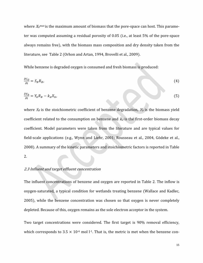
where Xbmax is the maximum amount of biomass that the pore-space can host. This parame-
ter was computed assuming a residual porosity of 0.05 (i.e., at least 5% of the pore-space
always remains free), with the biomass mass composition and dry density taken from the
literature, see Table 2 (Orhon and Artan, 1994, Brovelli et al., 2009).
While benzene is degraded oxygen is consumed and fresh biomass is produced:
, (4)
, (5)
where SB is the stoichiometric coefficient of benzene degradation, Yb is the biomass yield
coefficient related to the consumption on benzene and kd is the first-order biomass decay
coefficient. Model parameters were taken from the literature and are typical values for
field-scale applications (e.g., Wynn and Liehr, 2001; Rousseau et al., 2004, Gödeke et al.,
2008). A summary of the kinetic parameters and stoichiometric factors is reported in Table
2.
2.3 Influent and target effluent concentration
The influent concentrations of benzene and oxygen are reported in Table 2. The inflow is
oxygen-saturated, a typical condition for wetlands treating benzene (Wallace and Kadlec,
2005), while the benzene concentration was chosen so that oxygen is never completely
depleted. Because of this, oxygen remains as the sole electron acceptor in the system.
Two target concentrations were considered. The first target is 90% removal efficiency,
which corresponds to 3.5 × 10⁻⁶ mol l-1. That is, the metric is met when the benzene con-

16
centration in the discharged water is equal or smaller than 10% of the influent concentra-
tion (OEaux, 2008). Following the World Health Organization guidelines (World Health
Organization, 2006), a second and more restrictive target value was selected, equal to a
concentration of benzene of 0.01 mg l-1 (1.3 × 10⁻⁷ mol l-1). This value is conservative and is
the concentration limit for drinking water. While such a low value might be difficult to
achieve, it will be used to illustrate how the approach presented also allows the definition
of situations where the use of this wastewater treatment technology is not suitable due to a
high probability of failure.
2.4 Random hydraulic conductivity fields
The key feature of the design methodology is that the effect of heterogeneity is directly ad-
dressed making the hydraulic conductivity variable in space. Based on numerous case stu-
dies at the field and laboratory scales it is often assumed that hydraulic conductivity fol-
lows a log-normal distribution (e.g., Kottegoda and Katuuk, 1983; Hamed et al., 1996;
Skaggs and Barry, 1997). The two-dimensional hydraulic conductivity random field is often
parameterized using four variables, namely the mean and variance of the hydraulic conduc-
tivity distribution, and the correlation lengths in the longitudinal and transverse directions.
The mean and the variance control the interval in which the hydraulic conductivity can
vary. The correlation lengths and the ratio between the transverse and longitudinal length
scales (the aspect ratio of the field) instead define the spatial structure, a critical factor for
the HRTD. The effect of the correlation distances is exemplified in Fig. 1, where two realiza-
tions with different aspect ratios but same mean and variance are plotted. In both realiza-
tions the same transverse correlation length is used, and in both the longitudinal (horizon-

17
tal, in the direction of the flow) correlation is larger than in the transverse direction. In the
top panel, however, the aspect ratio is about 0.15, whereas in the bottom panel it is an or-
der of magnitude smaller (0.018). The comparison shows that, as the longitudinal correla-
tion increases (and so the aspect ratio decreases), the hydraulic conductivity field becomes
more stratified with horizontal flow paths tending to connect directly the inlet to the outlet.
This decreases the mixing of water in the porous bed and allows faster discharge of the pol-
luted water. When the longitudinal correlation is short compared to the scale of the wet-
land, the extent of the preferential flow paths is instead limited and good mixing (and
therefore high removal of the pollutants) is still possible.
The hydraulic conductivity fields were generated using a tool based on Mejia’s algorithm
(Mejia and Rodriguez-Iturbe, 1974) developed by Frenzel (1995) and included in the
PMWIN software (Processing Modflow for Windows) (Chiang, 2005). Twelve cases were
studied having different standard deviations and correlation lengths. However, only four
cases are informative so only those are reported and discussed in the following. A summary
of the features of the four random hydraulic conductivity fields is given Table 3. All the cas-
es had the same mean value (20 m d-1, consistent with the homogeneous case and corres-
ponds to a clean sand or sand/gravel porous medium, Bear and Verruijt, 1986), while the
standard deviation of the log-normal hydraulic conductivity distribution was varied. More
specifically, in two of the cases reported in the following the standard deviation was set to
10% of the mean hydraulic conductivity, while in the remainder it was set to 20% of the
mean. These values were selected to keep the resulting hydraulic conductivity in a reason-
able interval, as would be expected for a (relatively homogeneous) constructed wetland.
For example, when the standard deviation is 20% of the mean, the resulting hydraulic con-

18
ductivity varies in the range 0.1 to 120 m d-1. A larger interval is likely not realistic because
the porous media used as substrate for the treatment system are relatively coarse and the
grain size distribution is narrow. The only mechanism that might further alter the hydrau-
lic conductivity is biological activity (microbial growth, plant roots and rhizomes) that can
clog the pore space or create cracks and preferential flow paths. These processes were
however neglected in this work and therefore larger hydraulic conductivity ranges were
not considered.
The four cases considered all have the same correlation length in the transverse (vertical)
direction because it was found that this parameter had only a small influence on the HRTD.
The longitudinal correlation is instead more important, and the two values used were se-
lected to show the effect of a longitudinal correlation (i) shorter and (ii) comparable to the
size of the wetland in the flow direction.
Finally, it should be noted that while the method used in this work to create the random
hydraulic conductivity fields is one of the most popular, other approaches – sometimes
more sophisticated – are available. The design methodology presented is independent of
the approach used to generate heterogeneous distributions of the hydraulic properties.
3. Results and discussion
3.1 Conservative tracer and HRTD
Tracer experiments with continuous injection of a conservative non-retarded tracer were
simulated to study how heterogeneity affects the HRTD. Tracer BTCs are shown in Fig. 2,
where the normalized tracer concentration is reported as a function of the number of pore

19
volumes (PV). One PV corresponds to the nominal HRT, computed assuming homogeneous
conditions. The homogeneous case (named as Case H in this and following figures) is com-
pared with the two cases with short (left panel) and long (right panel) correlation lengths.
The homogenous case has a symmetric shape and almost no tailing, whereas the BTCs for
the heterogeneous cases indicate a more complex hydrodynamic behavior, suggested by
the longer tailing and the faster initial discharge. It is well known (e.g., Kreft and Zuber,
1978; Parker and van Genuchten, 1984; van Genuchten and Parker, 1984; Parlange et al.,
1985, 1992; Barry and Sposito, 1988) that the applied boundary conditions can have a
small effect on BTCs but it is clear from Fig. 2 that the medium heterogeneity has a much
more significant effect.
A convenient means to analyze the results in Fig. 2 is to convert the tracer BTCs in to the
corresponding HRTD (Fig. 3), computed as the time derivative of the normalized BTC. The
HRTD’s for heterogeneous conditions differ drastically to that for the homogeneous case. In
the homogeneous case the peak is symmetric and sharp, with a maximum that corresponds
to the nominal residence time (one PV). As the amount of heterogeneity increases (Cases 2
and 4) the position of the maximum is shifted towards shorter times, and both the spread-
ing and the skewness of the HRTD increase. The effect of heterogeneity on the residence
time can also be deduced from the computed effective (bulk) hydraulic conductivity of the
four cases. These values are given in Table 3, where the mean and standard deviation for
the 30 realizations are reported. For each realization the effective conductivity was com-
puted from the total water flow across the simulated wetland using Darcy’s law. The effec-
tive conductivity is larger than the mean value in all cases with heterogeneity, as expected
and as predicted from the BTCs. These results further stress the importance of the longitu-

20
dinal correlation length on the residence time because, with the same variance (cases 2 and
4), the effective hydraulic conductivity for the case where the longitudinal correlation
length is similar to the scale of the system is nearly twice that for the case with the short
correlation length.
The results of the simulations show that the values of both the variance and correlation
length produce different hydraulic conductivity patterns and hence BTCs. As the variance
of the log-normal distribution increases the hydraulic conductivity field can have larger
values, while a high longitudinal to vertical correlation length ratio (i.e., small aspect ratio)
tends to create preferential flow paths (see the random field shown in the lower panel of
Fig. 1 where high conductivity channels can be observed). The BTCs in Figs. 2 and 3 resem-
ble those that are produced by the two-region (or mobile-immobile region) model (e.g.,
Coats and Smith, 1964; Li et al., 1994; Griffioen et al., 1998). Indeed, Bajracharya and Barry
(1997) used a similar Monte Carlo approach to that presented here in order to relate em-
pirically the two-region model parameters to those of the hydraulic conductivity field.
Fig. 4 shows instead how the HRTD varies as the tracer moves from the inlet to the outlet in
the simulations with larger amount of heterogeneity. This figure shows the mean HRT
(50% of the mass of solute passed a given location) and the upper and lower 0.05 percen-
tiles, which indicate the time required for 5% and 95% of the mass of solute to pass
through a certain cross-section. In other words, for a certain cross-section, at the time indi-
cated by the upper 0.05 percentile, 95% of the mass of solute is still in between the inlet
and the cross-section, and vice-versa. In homogeneous conditions the HRT increases linear-
ly with the distance from the inlet (recall water flow is described using Darcy’s law) and is

21
controlled by the hydraulic conductivity. Fig. 4 confirms that even with heterogeneity the
HRT overall increases linearly as the water moves from the inlet to the outlet, although the
slope of the lower 0.05 percentile shows some limited variability. Consistent with the BTCs
in Fig. 3, the spreading of the HRTD is not symmetric around the mean value, as it would
tend to be for a homogeneous hydraulic conductivity. Moreover, the deviation from the
ideal, symmetric case (in other words, the skewness of the BTC) increases with the dis-
tance from the inlet. This indicates that the effect of heterogeneity is scale-dependent, as
already known theoretically (e.g., Dagan, 1984), in aquifers (e.g., Barry et al., 1988; Barry
and Sposito, 1990) and from the experimental findings of Suliman et al. (2005).
3.2 Biological transformations
Following the analysis of the changes in the HRTD resulting from heterogeneous distribu-
tion of the hydraulic properties, their effect on the microbial transformations was studied.
Fig. 5 reports the depth-averaged steady-state distribution of benzene, oxygen and biomass
in the constructed wetland. The simulated values were normalized using the initial concen-
tration for benzene, the maximum solubility for oxygen and the maximum amount of bio-
mass that the porous medium can host before becoming clogged (see §2.2). The focus of
this work is not to study benzene degradation in constructed wetlands, but to evaluate the
differences in terms of biological processes and contaminant degradation rate with and
without heterogeneity, and so simplifying modeling assumptions have been employed. In
particular, it is assumed that the only oxidizable component in the system is benzene, while
in reality other such components are likely to be present in the influent water. Fig. 5 com-
pares the results for the two cases with larger variance (Cases 2 and 4, respectively) with

22
the results obtained considering a homogeneous hydraulic conductivity. For the two cases
with heterogeneity the average value of the 30 realizations is reported (dashed line), as
well as the standard deviation (area shaded in gray). In the homogeneous case, three re-
gions are observed where the three components show similar behavior. In the first region
(fractional distance in the range 0 to about 0.2), the biomass density is constant and is
equal to the maximum value (defined by the available pore-space, see Eqs. 2 and 3). Since
biomass cannot grow any further benzene and oxygen are exclusively consumed to replace
the biomass undergoing cellular lysis. Therefore, the consumption rates are constant (re-
call biomass decay is modeled as a first-order kinetic process), and the concentration of
both oxygen and benzene decrease linearly. In the second region (in the range 0.2 to 0.25 of
relative distance from the inlet) the three components show a sharp decay. In this part of
the system biomass growth is not limited by the pore space availability (i.e., ), the
concentrations are such that the biomass growth and decay rates are in equilibrium, and
therefore both oxygen and benzene are quickly depleted and the concentration of the sub-
strate drops by about one order of magnitude within about 0.1 m. This is due to the rather
high maximum degradation rate. In the third region, from 0.25 to the outlet, the concentra-
tions of the three components show a very smooth variation, because the availability of
both benzene and oxygen becomes the factor limiting the biodegradation rate. The oxygen
concentration is reduced to about 10% of the initial value (the solubility limit) but is not
completely depleted, i.e., the system never becomes strictly anaerobic.
Simulations with heterogeneity show very different behavior. In both models (Case 2 and
4), the change in concentration of the three components with the distance from the inlet is
smoother, and biomass growth near the inlet is reduced compared to the homogeneous

23
case. The standard deviation generally increases with the distance from the inlet, and be-
comes very large for benzene (and oxygen) in Case 4. This means that the same change in
flow or HRT (the heterogeneity is statistically homogeneous within the wetland and among
the different realizations) has a stronger impact when the degradation rate is reduced, and
indicates that systems designed to treat recalcitrant compounds are more sensitive to hete-
rogeneity than systems where the substrate is easily biodegraded.
The steady-state depth-averaged profiles cannot be easily explained considering the bio-
logical processes only, as was done for the homogeneous case. In the heterogeneous case
the spatial distribution of solutes and biomass is controlled by the flow patterns. This can
be observed in Fig. 6, where an example of the real biomass distribution in the simulations
with heterogeneity is shown. Once again, in this plot the biomass is normalized using the
maximum biomass density that the porous medium can host. Fig. 6 shows that biomass
developed in a complex and unpredictable pattern, with variations as large as two orders of
magnitude in the transverse direction. The biomass distribution map reported here is rele-
vant to Case 2, which has large variance and small longitudinal correlation length. A visual
comparison with the biomass distribution for Case 4 (large correlation length, not shown)
revealed that the biomass growth pattern is controlled by the aspect ratio of the hydraulic
conductivity field, although in a non-trivial way, and a more quantitative comparison would
be difficult.
These findings raise a number of questions regarding the representativeness of samples
taken in constructed wetlands with a heterogeneous substrate and regarding the quantita-
tive understanding of the biological processes in such systems. The strong changes in bio-

24
mass density in the direction transversal to the flow field suggest that use of limited sam-
pling locations in the vertical direction is likely to be uninformative regarding the real bio-
mass distribution. It should also be noted that in these simulations, as previously discussed,
the transverse direction was neglected. However, it can be expected that the same variabili-
ty observed in Fig. 6 could also be found in the transverse (horizontal) direction, since the
underlying governing mechanisms are the same. This implies that, if reliable information
regarding the spatial distribution of biomass (or any other component) is sought, a dense
grid of sampling locations must be used to characterize each cross-section. In terms of
process understanding, the results of our simulations indicate that the measured values are
difficult to compare or be used as input in models. Model simulations are often calibrated
or compared using the average of the measurements in a cross-section transverse to the
flow direction. Since biological transformations are strongly non-linear processes – the si-
mulation results show that the components can vary over one order of magnitude in a li-
mited distance – it is questionable whether the use, e.g., of the arithmetic mean is the best
choice to average the measurements. It should also be considered that in all the simulations
reported here, while biomass growth is limited by the amount of available pore space the
plugging of the pores does not affect the hydraulic properties. In other words, in heteroge-
neous conditions it is expected that biomass grows first in the high conductivity zones
where the solutes are more quickly replaced. The growth of biomass reduces however the
local hydraulic conductivity thus promoting a reduction of the heterogeneity. While this
mechanism is likely, previous simulations (Brovelli et al., 2009) have shown that – at least
in some conditions – clogging can further promote the increase in heterogeneity and the
formation of new preferential flow paths.

25
To summarize, simulation results indicate that the presence of physical heterogeneities in
the porous substrate induce the development of complex distribution patterns of both the
mobile (solutes) and immobile components (biomass) that complicate the understanding
of the processes and might reduce the overall biodegradation rate. The interactions and
feedback between the different mechanisms taking place have however not been studied
yet, and predictions are complicated by the non-linearity of the biological processes.
3.3 Treatment efficiency and design methodology
The results presented and discussed above indicate that heterogeneity affects the contami-
nant degradation rate. To gain additional insights into this aspect, we have analyzed simu-
lation results considering the target concentrations defined in §2.3 above, namely the WHO
concentration for benzene in drinking water, and the 90% removal efficiency. Results are
reported in Fig. 7, where the average benzene concentrations of the 30 realizations for Cas-
es 1 to 4 are shown as a function of the nominal HRT in the wetland, i.e., the residence time
assuming that the hydraulic conductivity is constant. The results in heterogeneous condi-
tions are compared with the simulated benzene profile obtained using a homogeneous
porous medium (solid line in Fig. 7). Clearly, in all the cases with heterogeneity the two
target concentrations are achieved with a longer HRT, and in some cases are not met. Recall
that the values shown in Fig. 7 are the average values of the 30 realizations, meaning that
for some of the realizations the target concentrations are achieved. This is important and
will be further discussed in the following. In terms of design methodology, Fig. 7 can be
used to identify the THRT already introduced and discussed in the methodology section.
For benzene degradation considered here, the THRT for the 90% removal and WHO limit

26
are about 2.0 d and 6.5 d (noted as THRT(1) and THRT(2) in Fig. 7). It is interesting to note
that, due to the non-linear behavior of the microbial processes the additional benzene de-
gradation to reach the WHO limit from the 90% degradation requires more than twice the
time required to remove 90% of the initial benzene concentration.
The THRT can be used to identify the optimal inlet flow rate or the hydraulic gradient, us-
ing a tracer experiment conducted to characterize the HRTD and computing subsequently
the flow velocity in the wetland’s bed necessary to achieve a certain mean HRT. Further-
more, the approach we have presented is a powerful methodology to design constructed
wetlands including the effect of heterogeneity. The results of the stochastic simulations are
easily converted into the PFS for a given level of heterogeneity. For the setup considered in
this work, the PFS is presented in Fig. 8. The panel on the left shows the PFS for 90% ben-
zene removal, whereas the plot on the right is relevant to the WHO limit. For a given cross-
section in the flow direction, the PFS is the ratio between the number of realizations for
which the target concentration is achieved and the total number of realizations. The dis-
crete values (not shown) were subsequently fitted using a logistic curve to obtain a conti-
nuous probability function. According to Fig. 8, the PFS for the setup considered in this
work reaches 0 after 7 d unless the heterogeneity is large (i.e., the variance of the hydraulic
conductivity is large) and the correlation length of the hydraulic conductivity field is com-
parable to the size of the wetland. Even in this case however, the PFS is only limited (about
20%). Since the correlation length depends primarily on the filling strategy (e.g., Suliman et
al., 2007), it can in principle be controlled and reduced using an appropriate methodology
during the construction phase. In other words, except for the case with large heterogeneity,
the system considered would be able to remove 90% of the contaminant with a nominal

27
HRT of about 7 d. On the other hand, the system used here is not suitable to reach the WHO
limit unless the hydraulic conductivity variability can be limited (e.g., by carefully selecting
the grain size distribution of the porous material) and the correlation length minimized.
4. Summary and conclusions
The effect of the porous medium physical heterogeneity on the HRTD of horizontal subsur-
face flow constructed wetlands and sand filters was analyzed by means of numerical simu-
lations. Heterogeneity was included in the simulated domain using random spatially corre-
lated hydraulic conductivity fields. The extent of heterogeneity was controlled by the va-
riance of the hydraulic conductivity distribution and by the correlation length in the flow
direction. It was observed that substrate heterogeneity induces preferential flow paths,
modifies the HRTD and results in variations of the treatment efficiency. Simulated tracer
tests conducted to characterize the residence time distribution showed that as the extent of
the heterogeneity increases (increase in variance and longitudinal correlation length simi-
lar to the size of system) the mean HRT decreases, the HRTD becomes broader and its
skewness increases. Moreover, scale-dependent behavior was observed: The sensitivity of
the HRTD to heterogeneity was larger when the correlation length was comparable to the
dimensions of the system. In other words, if the system is large compared to the scale at
which the hydraulic conductivity varies the effect of heterogeneity is limited. Similar ob-
servations were made regarding the effect of heterogeneity on the removal rate. Further-
more, and possibly more important, it was found that the microbial growth patterns are
affected by the flow field, and that as heterogeneity increases the biomass spatial distribu-
tion becomes more complex and the removal rate shows larger variability (as shown by the

28
increase in the standard deviation in Fig. 5). These insights on the biomass distribution
indicate that collection of a limited number of samples in the transverse directions is of
limited use because the representativeness of few samples is small.
The approach presented in this work is a possible design methodology for constructed wet-
lands, in that the effect of heterogeneity can be incorporated in a quantitative manner. The
methodology is based on the use of numerical tools to simulate solute transport and biode-
gradation, and therefore requires knowledge of the processes involved, including their pa-
rameterization. On the other hand, a process-based design can prove extremely helpful in
reducing the sources of uncertainty, therefore improving the treatment efficiency and re-
liability of the system. In this respect, detailed mechanistic simulators are of increased im-
portance. The key advantage of the approach is that it uses a stochastic methodology to
evaluate the effect of heterogeneity on removal rate and the HRTD. For a given configura-
tion of the wetland, multiple realizations of statistically equivalent hydraulic conductivity
random fields are generated. This is a standard technique used in subsurface hydrology,
and its application to CWs is straightforward. This approach allows the computation of the
probability of failure of the system as a function of the HRT. The optimal dimension of the
system can subsequently be decided based on the expected flow rate, its variations and the
probability of failure that can be tolerated. For example, if the water body receiving the
water discharged from the treatment plant is very sensitive, a low probability of failure is
required even for the maximum expected loading rate of the system, and the system must
be dimensioned accordingly. Although the approach presented in this work makes use of
tools that might not common in the constructed wetland community, it should be clear that
they are available and their diffusion and use might be extremely beneficial to overcome

29
some of the major limitations of CWs. Moreover, it is important to note that this same me-
thodology can be further extended to incorporate additional sources of variability and un-
certainty, for example those affecting the degradation rates of the contaminants (tempera-
ture, loading rate, etc.), therefore making the design phase more reliable and effectively
process-based. In other words, every aspect showing some level of stochastic variability
can be modeled within the same framework, given that the statistical properties of the ran-
dom process are known. However, to be able to extend the method in this direction, the use
of more sophisticated simulators is required and therefore more research is required.

30
References
Akratos, C.S., Tsihrintzis, V.A., 2007. Effect of temperature, HRT, vegetation and porous me-
dia on removal efficiency of pilot-scale horizontal subsurface flow constructed wet-
lands. Ecol. Eng. 29 (2), 173–191.
Alagappan, G., Cowan, R.M., 2004. Effect of temperature and dissolved oxygen on the
growth kinetics of Pseudomonas putida F1 growing on benzene and toluene.
Chemosphere 54 (8), 1255–1265.
Ascuntar-Rios, D., Toro-Vélez, A.F., Peña, M.R., Madera-Parra, C.A., 2009. Changes of flow
patterns in a horizontal subsurface flow constructed wetlands treating domestic waste-
water in tropical regions. Ecol. Eng. 35 (2), 274–280.
Bajracharya, K., Barry, D.A., 1997. Nonequilibrium solute transport parameters and their
physical significance: Numerical and experimental results. J. Contam. Hydrol. 24 (3-4),
185–204.
Barnett, V., O’Hagan, A. 1997. Setting environmental standards: the statistical approach to
handling uncertainty and variation. Chapman & Hall, London, p. 112.
Barry, D.A., 1990. Supercomputers and their use in modeling subsurface solute transport.
Rev. Geophys., 28 (3), 277–295.
Barry, D.A., Coves, J., Sposito, G., 1988. On the Dagan model of solute transport in ground-
water: Application to the Borden site. Water Resour. Res., 24 (10), 1805–1817.

31
Barry, D.A., Prommer, H., Miller, C.T., Engesgaard, P., Brun, A., Zheng, C., 2002. Modelling the
fate of oxidisable organic contaminants in groundwater. Adv. Water Resour., 25 (8-12),
945–983.
Barry, D.A., Sposito, G., 1988. Application of the convection-dispersion model to solute
transport in finite soil columns. Soil Sci. Soc. Am. J., 52 (1), 3–9.
Barry, D.A., Sposito, G., 1990. Three-dimensional statistical moment analysis of the Stan-
ford/Waterloo Borden tracer data. Water Resour. Res., 26 (8), 1735–1747.
Bear, J., Verruijt, A., 1986. Modeling groundwater flow and pollution, with computer pro-
grams for sample cases, D. Reidel Publ. Co., Dordrecht, Germany, p. 414.
Bedessem, M.E., Ferro, A.M., Hiegel, T., 2007. Pilot-scale constructed wetlands for petro-
leum-contaminated groundwater. Water Environment Research 79, 581–586. Brix, H.,
Arias, C.A., 2005. Danish guidelines for small-scale constructed wetland systems for on-
site treatment of domestic sewage. Water Sci. Technol. 15 (9), 1–9.
Brovelli, A., Malaguerra, F., Barry, D.A., 2009. Bioclogging in porous media: Model develop-
ment and sensitivity to initial conditions. Environ. Model. Softw. 24 (5), 611–626.
Caselles-Osorio, A., García, J., 2006. Performance of experimental horizontal subsurface
flow constructed wetlands fed with dissolved or particulate organic matter. Water Res.
40 (19), 3603–3611.
Chazarenk, F., Merlin, G., Gonthier, Y., 2003. Hydrodynamics of horizontal subsurface flow
constructed wetlands. Ecol. Eng. 21 (2-3), 165–173.

32
Chiang, W.H., 2005. 3D groundwater modeling with PMWIN, 2nd ed. Springer-Verlag, The
Netherlands, p. 397.
Chin, D.A., 2006. Water quality engineering in natural systems. Wiley-Interscience, NJ, USA,
p. 610.
Coats, K.H., Smith, B.D., 1964. Dead-end pore volume and dispersion in porous media. Soc.
Petrol. Eng. J., 4 (3), 73–84.
Dagan, G., 1984. Solute transport in heterogeneous porous formations. J. Fluid Mech., 145,
151–177.
Dagan, G., 1989. Flow and Transport in Porous Formations, Springer-Verlag, Berlin, Ger-
many. p. 465.
Dittmer, U., Meyer, D., Langergraber, G., 2005. Simulation of a subsurface vertical flow con-
structed wetland for CSO treatment. Water Sci Technol 51(9), 225–232.
Eke, P.E., Scholz, M., 2008. Benzene removal with vertical-flow constructed treatment wet-
lands. Journal of Chemical Technology and Biotechnology 83, 55–63.
Frenzel, H., 1995. A field generator based on Mejia’s algorithm. Institut für Umweltphysik,
University of Heidelberg, Germany.
García, J., Chiva, J., Aguirre, P., Álvarez, E., Sierra, J.P., Mujeriego, R., 2004. Hydraulic beha-
vior of horizontal subsurface flow constructed wetlands with different aspect ratio and
granular medium size. Ecol. Eng., 23 (3), 177–187.

33
Gelhar, L.W., Welty C., Rehfeldt K.R., 1992. A critical review of data on field-scale dispersion
in aquifers. Water Resour. Res., 28 (7), 1955–1974.
Giraldi, D., de Michieli Vitturi, M., Iannelli, R., 2010. FITOVERT: A dynamic numerical model of sub-
surface vertical flow constructed wetlands. Environ. Model. Software. 25 (5), 633–640.Gödeke,
S., Vogt, C., Schirmer, M., 2008. Estimation of kinetic Monod parameters for anaerobic
degradation of benzene in groundwater. Environ. Geol., 55 (2), 423–431.
Griffioen, J.W., Barry, D.A., Parlange. J.-Y., 1998. Interpretation of two-region model parame-
ters. Water Resour. Res., 34 (3), 373–384.
Grismer, M.E., Tausendschoen, M., Shepherd, H., 2001. Hydraulic characteristics of a sub-
surface flow constructed wetland for winery effluent treatment. Water Environ. Res., 73
(4), 466–477.
Haberl, R., Grego, S., Langergraber, G., Kadlec, R.H., Cicalini, A.R., Dias, S.M., Novais, J.M.,
Gerth, A., Thomas, H., Hebner, A., 2003. Constructed wetlands for treatment of organic
pollutants. J. Soils Sediments, 3 (2), 109–124.
Hamed, M.M., Bedient, P.B., Dawson, C.N., 1996. Probabilistic modeling of aquifer hetero-
geneity using reliability methods. Adv. Water Resour., 19 (5), 277–295.
Hench, K.R., Bissonnette, G.K., Sexstone, A.J., Coleman, J.G., Garbutt, K., Skousen, F.G., 2003.
Fate of physical, chemical, and microbial contaminants in domestic wastewater follow-
ing treatment by small constructed wetlands. Water Res., 37 (4), 921–927.

34
Hristopulos, D.T., 2003. Renormalization group methods in subsurface hydrology: Over-
view and applications in hydraulic conductivity upscaling. Adv. Water Resour., 26 (12),
1279–1308.
Imfeld, G., Braeckvelt, M., Kuschk, P., Richnow, H., 2009. Monitoring and assessing
processes of organic chemicals removal in constructed wetlands. Chemosphere, 74 (3)
349–362.
Jenkins, G.A., Greenway, M., 2005. The hydraulic efficiency of fringing versus banded vege-
tation in constructed wetlands. Ecol. Eng., 25(1), 61–72.
Johnson, S.J., Woolhouse, K.J., Prommer, H., Barry, D.A., Christofi. N., 2003. Contribution of
anaerobic microbial activity to natural attenuation of benzene in groundwater. Eng.
Geol., 70 (3-4), 343–349.
Kadlec, R.H. 1997. Deterministic and stochastic aspects of constructed wetland perfor-
mance and design. Water Sci. Technol., 35(5), 149–159.
Kadlec, R.H., 2003. Effects of pollutant speciation in treatment wetlands design. Ecol. Eng.,
20 (1), 1–16.
Kadlec, R.H., 2009. Comparison of free water and horizontal subsurface treatment wet-
lands. Ecol. Eng., 35 (2), 159–174.
Kadlec, R.H., Wallace, S.D., 2009. Treatment Wetlands, 2nd ed. CRC Press, Boca Raton, FL,
USA, p. 1016.

35
Kamra, S.K., Lennartz, B., van Genuchten, M.Th., Widmoser, P., 2001. Evaluating non-
equilibrium solute transport in small soil columns. J. Contam. Hydrol., 48 (3-4), 189–
212.
King, A.C., Mitchell, C.A., Howes, T., 1997. Hydraulic tracer studies in a pilot scale subsurface
flow constructed wetland. Water Sci. Technol., 35(5), 189–196.
Kjellin, J., Wörman, A., Johansson, H., Lindahl, A., 2007. Controlling factors for water resi-
dence time and flow patterns in Ekeby treatment wetland, Sweden. Adv. Water Resour.,
30 (4), 838–850.
Knowles, P.R., Griffin, P., Davies, P.A., 2008. An investigation into the development of hete-
rogeneous hydraulic conductivity profiles in constructed wetlands for wastewater
treatment. 11th International Conference on Wetland Systems for Water Pollution Con-
trol IWA. Indore, India. pp. 814–824.
Kottegoda, N.T., Katuuk, G.C., 1983. Effect of spatial variation in hydraulic conductivity on
groundwater flow by alternate solution techniques. J. Hydrol., 65 (4), 349–362.
Kreft, A., Zuber, A., 1978. On the physical meaning of the dispersion equation and its solu-
tions for different initial and boundary conditions. Chem. Eng. Sci., 33 (11), 1471–1480.
Langergraber, G., 2003. Simulation of subsurface flow constructed wetlands- Results and
further research needs. Water Sci. Technol. 48, 157–166.
Langergraber, G., 2007. Simulation of the treatment performance of outdoor subsurface
flow constructed wetlands in temperate climates. Sci. Total Environ. 380, 210–219.

36
Langergraber, G., 2008. Modeling of processes in subsurface flow constructed wetlands: A
review. Vadose Zone Journal. 7, 830–842.
Langergraber, G., Giraldi, D., Mena, J., Meyer, D., Peña, M., Toscano, A., Brovelli, A., Korkusuz,
E.A., 2009a. Recent developments in numerical modelling of subsurface flow constructed
wetlands. Sci. Total Environ., 407 (13), 3931–3943.
Langergraber, G., Rousseau, D.P., Garcia, J., Mena, J., 2009b. CWM1: a general model to de-
scribe biokinetic processes in subsurface flow constructed wetlands. Water Sci. Technol.
59, 1687–1697.
Leverenz, H.L., Tchobanoglous, G., Darby, J.L., 2009. Clogging in intermittently dosed sand
filters used for wastewater treatment. Water Res., 43 (3), 695–705.
Lewis, M.E., 2006. Dissolved oxygen. U.S. Geological Survey Techniques of Water-Resources
Investigations, book 9, chap. A6.
Li, L., Barry, D.A., Stone, K.J.L., 1994. Centrifugal modelling of nonsorbing, nonequilibrium
solute transport in a locally inhomogeneous soil. Canad. Geotech. J., 31 (4), 471–477.
Lin, T., Wen, Y., Jiang, L., Li, J., Yang, S., Zhou, Q., 2008. Study of atrazine degradation in sub-
surface flow constructed wetland under different salinity. Chemosphere, 72 (1), 122–
128.
McDonald, M., Harbaugh, A., 1988. A Modular Three-Dimensional Finite-Difference Ground-
Water Flow Model. U.S Geological Survey, USA.

37
Małoszewski P. Wachniew P. Czuprynski P. 200 . Study of hydraulic parameters in hete-
rogeneous gravel beds: Constructed wetland in Nowa Slupia (Poland). J. Contam. Hy-
drol., 331 (3-4), 630–642.
Mao, X., Prommer, H., Barry, D.A., Langevin, C., Panteleit, B. 2006. Three-dimensional model
for multi-component reactive transport with variable density groundwater flow. Envi-
ron. Model. Softw., 21 (5), 615–628.
Marsili-Libelli, S., Checchi, N., 2005. Identification of dynamic models for horizontal subsur-
face constructed wetlands. Ecol. Model., 187, 201–218.
Matamoros, V., Bayona, J.M., 2006. Elimination of pharmaceutical and personal care prod-
ucts in subsurface flow constructed wetlands. Environ. Sci. Technol., 40 (18), 5811–
5816.Matamoros, V., Puigagut, J., García, J., Bayona, J.M., 2007a. Behavior of selected
priority organic pollutants in horizontal subsurface flow constructed wetlands: A pre-
liminary screening. Chemosphere, 69 (9), 1374–1380.
Mayo, A.W., Bigambo, T., 2005. Nitrogen transformation in horizontal subsurface flow con-
structed wetlands I: Model development. Physics and Chemistry of the Earth. 30, 658–
667.
Matamoros, V., Arias, C., Brix, H., Bayona, J.M., 2007b. Removal of pharmaceuticals and per-
sonal care products (PPCPs) from urban wastewater in a pilot vertical flow con-
structed wetland and a sand filter. Environ. Sci. Technol., 41 (23), 8171–8177.

38
Matamoros, V., García, J., Bayona, J.M., 2008. Organic micropollutant removal in a full-scale
surface flow constructed wetland fed with secondary effluent. Water Res., 42 (3), 653–
660.
McGechan, M.B., Moir, S.E., Castle, K., Smit, I.P.J., 2005. Modelling oxygen transport in a
reedbed-constructed wetland purification system for dilute effluents. Biosyst. Engin.
91, 191–200.
Mejia J.M., Rodriguez-Iturbe I., 1974. On the synthesis of random field sampling from the
spectrum: An application to the generation of hydrologic spatial processes. Water Re-
sour. Res., 10 (4), 705–711.
Mena, J., Gómez, R., Villaseñor, J., De-Lucas, A., 2008. Operation time influence on con-
structed wetlands hydraulic. 11th International Conference on Wetland Systems for Wa-
ter Pollution Control IWA. Indore, India, p. 445.
Moore, B.J., Lyness, L.S., Ross, S.D., Armstrong, J.E., Bowles, M.W., 2000. Innovative ap-
proaches for the remediation of petroleum hydrocarbons in groundwater, 16th World
Petroleum Congress, Calgary, Canada, pp. 46–48.
Muñoz, P., Drizo A., Hession, C., 2006. Flow patterns of dairy wastewater constructed wet-
lands in a cold climate. Water Res., 40 (17), 3209–3218.
OEaux, 2008. Swiss Federal Ordinance for water protection (In French, Ordonnance sur la
protection des eaux), RS 814.201, Swiss legislation, Bern, Switzerland.
Orhon, D., Artan, N., 1994. Modelling of activated sludge systems. Technomic Publishing
Company, Inc., Lancaster, Pennsylvania, USA, p. 589.

39
Parker J.C., van Genuchten M.Th., 1984. Flux-averaged and volume-averaged concentra-
tions in continuum approaches to solute transport. Water Resour. Res., 20 (7), 866–872.
Parlange, J.-Y., Barry, D.A., Starr, J.L., 98 . Comments on “Boundary conditions for dis-
placement experiments through short laboratory soil columns”. Soil Sci. Soc. Am. J., 49
(5), 1325.
Parlange, J.-Y., Starr, J.L., van Genuchten, M.Th., Barry, D.A., Parker, J.C., 1992. Exit condition
for miscible displacement experiments. Soil Sci., 153 (3), 165–171.
Persson, J., Somes, N.L.G., Wong, T.H.F., 1999. Hydraulic efficiency of constructed wetlands
and ponds. Water Sci. Technol., 40 (3), 291–300.
Prommer, H., Barry, D.A., 2005. Modeling bioremediation of contaminated groundwater. In:
Atlas, R., Philip, J.C. (Eds.), Bioremediation: Applied microbial solutions for real-world
environmental clean-up, pp. 108–138. AMS Press, American Society for Microbiology.
Washington, DC, USA.
Prommer, H., Barry, D.A., Davis, G.B., 1999. A one-dimensional reactive multi-component
transport model for biodegradation of petroleum hydrocarbons in groundwater. Envi-
ron. Model. Softw., 14 (2-3), 213–223.
Prommer, H., Barry, D.A., Davis, G.B., 2000. Numerical modelling for design and evaluation
of groundwater remediation schemes. Ecol. Model., 128 (2-3), 181–195.
Rash, J.K., Liehr, S.K., 1999. Flow pattern analysis of constructed wetlands treating landfill
leachate. Water Sci. Technol., 40 (3), 309–315.

40
Reiche, N., Lorenz, W., Borsdorf, H., 2010. Development and application of dynamic air
chambers for measurement of volatilization fluxes of benzene and MTBE from con-
structed wetlands planted with common reed. Chemosphere 79, 162–168.Reinoso, R.,
Torres, L.A., Bécares, E., 2008. Efficiency of natural systems for removal of bacteria and
pathogenic parasites from wastewater. Sci. Total Environ., 395 (2-3), 80–86.
Robinson, C., Brovelli, A., Barry, D.A., Li, L., 2009. Tidal influence on BTEX biodegradation in
sandy coastal aquifers. Adv. Water Resour., 32 (1), 16–28.
Rossi L., Chèvre N., Fankhauser R., Krejci V. (2009) Probabilistic environmental risk as-
sessment of urban wet-weather discharges: an approach developed for Switzerland. Ur-
ban Water J., 6 (5), 355–367.
Rousseau, D.P.L., Vanrolleghem, P.A., De Pauw, N., 2004. Model-based design of horizontal
subsurface flow constructed treatment wetlands: A review. Water Res., 38 (6), 1484–
1493
Schirmer, M., Molson, J.W., Frind, E.O., Barker, J.F., 2000. Biodegradation modelling of a dis-
solved gasoline plume applying independent laboratory and field parameters. J. Contam.
Hydrol., 46, 339–374.
Skaggs, T. H., Barry, D.A., 1997. The first-order reliability method of predicting cumulative
mass flux in heterogeneous porous formations. Water Resour. Res., 33 (6), 1485–1494.
Sposito, G., Barry, D.A., 1987. On the Dagan model of solute transport in groundwater:
Foundational aspects. Water Resour. Res., 23 (10), 1867–1875.

41
Stott, R., Warren, A., Williams, J., Ramirez, E., 2008. The removal of pathogens and parasites
in sub-surface flow constructed wetlands treating wastewaters in Egypt, Mexico and the
UK. 11th International Conference on Wetland Systems for Water Pollution Control IWA.
Indore, India, p. 782.
Suliman, F., Futsaether, C., Oxaal, U., 2007. Hydraulic performance of horizontal subsurface
flow constructed wetlands for different strategies of filling the filter medium into the fil-
ter basin. Ecol. Eng., 29 (1), 45–55.
Suliman, F. Futsaether, C., Oxaal, U., Haugen L.E., Jenssen, P., 2006a. Effect of inlet-outlet
positions on the hydraulic performance of horizontal subsurface-flow wetlands con-
structed with heterogeneous porous media. J. Contam. Hydrol., 87 (1-2), 22–36.
Suliman, F., French, H.K., Haugen, L.E., Sovik, A.K., 2006b. Change in flow and transport pat-
terns in horizontal subsurface flow constructed wetlands as a result of biological
growth. Ecol. Eng., 27 (2), 124–133.
Suliman, F., French, H., Haugen, L.E., Klove, B., Jenssen, P., 2005. The effect of the scale of
horizontal subsurface flow constructed wetlands on flow and transport parameters. Wa-
ter Sci. Technol., 51 (9), 259–266.
Tang, X., Eke, P.E., Scholz, M., Huang, S., 2008. Processes impacting on benzene removal in
vertical-flow constructed wetlands. Bioresource Technology 100, 227–234.
Tang, X., Eke, P.E., Scholz, M., Huang, S., 2009. Seasonal variability in benzene removal by
vertical-flow constructed wetland filters. Water, Air, and Soil Pollution 202, 259–272.

42
Toscano, A., Langergraber, G., Consoli, S., Cirelli, G.L., 2009. Modelling pollutant removal in a
pilot-scale two-stage subsurface flow constructed wetlands. Ecol. Eng. 35, 281–289.
van Genuchten, M.Th., Parker, J.C., 1984. Boundary conditions for displacement experi-
ments through short laboratory soil columns. Soil Sci. Soc. Am. J., 48 (4), 703–708.
Vymazal, J., 2007. Removal of nutrients in various types of constructed wetlands. Sci. Total
Environ., 380 (1-3), 48–65.
Vymazal, J., Kröpfelová, L., 2008. Wastewater treatment in constructed wetlands with hori-
zontal sub-surface flow. Series Environmental Pollution, vol 14. Springer-Verlag, The
Netherlands, p. 566.
Wallace, S., Kadlec, R., 2005. BTEX degradation in cold-climate wetland system. Water Sci.
Technol., 51 (9), 165–171.
Wallace, S.D., 2001. On-site remediation of petroleum contact wastes using subsurface flow
wetlands. Procs 2nd int. conf. wetlands and remediation. Vermont, USA.
World Health Organization. Guidelines for drinking-water quality, vol. 1, recommendations
2006.
Wörman, A., Kronnäs, V., 2005. Effect of pond shape and vegetation heterogeneity on flow
and treatment performance of constructed wetlands. J. Hydrol., 301, 123–138
Wynn, T.M., Liehr, S.K., 2001. Development of a constructed subsurface-flow wetland simu-
lation model. Ecol. Eng., 16 (4), 519–536.

43
Zheng, C., Wang, P., 1999. MT3DMS, a Modular Three-Dimensional Multi-Species Transport
Model for Simulation of Advection, Dispersion and Chemical Reactions of Contaminants
in Ground-Water Systems; Documentation and User’s Guide. U.S. Army Engineer Re-
search and Development Center, USA.

44
Tables
Table 1. Main features of the constructed wetland model. Typical values for subsurface flow
constructed wetlands for secondary treatment were used (e.g., Brix and Arias, 2005; Chin,
2006; Kadlec and Wallace, 2009). The hydraulic conductivity listed in this table is relevant
to the case with homogenous porous medium.
Property Value Units
Length 10 m
Depth 1 m
Nominal residence time(a) 9.5 d
Porosity 0.38 -
Hydraulic conductivity(b) 20 m d-1
Hydraulic gradient 2 × 10⁻² -
Longitudinal dispersivity 2 × 10⁻² m
(a)Based on the expected seepage velocity and the size of the system
(b)The same value was used for both vertical and horizontal hydraulic conductivity

45
Table 2. Stoichiometry and Monod kinetic parameters for the aerobic degradation of ben-
zene. Also listed are the influent concentrations of benzene and oxygen, and the initial bio-
mass concentration.
Parameter Value Units Source
µmax,B 1 d-1 Average value(a)
KS,B 3 × 10⁻² mmol l-1 Alagappan and Cowan (2004)
Yb 6 × 10⁻¹ - Alagappan and Cowan (2004)
KS,O 3.6 × 10⁻² mmol l-1 Alagappan and Cowan (2004)
SB 7.5 (mol O2)(mol C6H6)-1
Stoichiometry, Eq. (1)
kd 10-3 d-1 Assumed(b)
Benzene(c) 3.5 × 10⁻² mmol l-1 Assumed
Oxygen(c) 28.7 × 10⁻² mmol l-1 Solubility limit at 20°C (Lewis, 2006)
Biomass(c) 3 × 10⁻² mmol l-1 Assumed
Xbmax 2 mmol l-1 Computed using literature value(d)
(a)From Schirmer et al. (2000) and Gödeke et al. (2008).
(b)A small value is used for the first-order biomass decay rate because in reality microbial
growth is supported by alternative carbon and energy sources, which are not included in
the model
(c)Influent concentration
(d)Orhon and Artan (1994); Brovelli et al. (2009).

46
Table 3. Summary of the properties of the hydraulic conductivity fields in the four cases
discussed in the text, as well as the homogeneous case. The effective (bulk) hydraulic con-
ductivity K is the average (±1 standard deviation) of the 30 realizations.
Case Hydraulic conductivity(a) Correlation length (m) Effective K (m d-1)
Mean value (m d-1)
Variance (m2 d-2)
Longitudinal Vertical
H(b) 20 - - - 20
1 20 4 1 0.15 22.05 ± 0.64
2 20 16 1 0.15 27.62 ± 3.77
3 20 4 8 0.15 24.59 ± 0.60
4 20 16 8 0.15 50.72 ± 6.63
(a)Parameters of the log-normal distribution (base 10)
(b)Homogeneous (base) case. The hydraulic conductivity is constant

47
Figures
Figure 1. Example of heterogeneous hydraulic conductivity random fields used in the simu-
lations. The mean, the variance and the vertical correlation length are the same in the two
panels. The x and y axes are scaled by the real dimensions. The longitudinal correlation
length is small compared to model size in the top panel, while is comparable to the dimen-
sion of the system in the bottom panel, leading to a vertically stratified system (e.g., Sposito
and Barry, 1987).

48
Figure 2. Simulated BTCs of the conservative tracer with homogenous (Case H, solid line)
and heterogeneous (broken lines) porous media. The average breakthrough of 30 realiza-
tions is shown. On the left panel (a) the homogeneous case is compared with cases 1 and 2,
while on the right panel (b) the BTCs for cases 3 and 4 are reported (see Table 3 for details
regarding the statistical properties of the conductivity fields). The simulation results indi-
cate that heterogeneity modifies the HRTD. The mean HRT decreases while the spreading is
accentuated. This indicates that hydraulic conditions are less favorable for degradation
then the homogeneous case.

49
Figure 3. HRTDs for the simulations with constant hydraulic conductivity (solid line) and
with spatially variable hydraulic properties (broken lines). Panels (a) and (b) show the
results for short and long correlation lengths, respectively. The HRTD is sharp and symme-
tric with the peak corresponding to the nominal retention time (one pore volume) only for
the homogeneous case. Increasing the variance and the correlation length of the conductiv-
ity field leads to a reduction in the mean HRT while both the variance and skewness of the
HRTD increase.

50
Figure 4. Evolution of HRTD as function of the distance from the inlet for the worst case
(i.e., large variance and correlation length, Case 4). For a wetland of length of, say, 4 m, the
dashed line indicates that, of the solute flowing through the system, 95% will experience
an HRT of, approximately, at least 1 d, 50% at least 2 d and 5% at least 9 d. Despite the
large heterogeneity, the evolution of the mean HRT (50% mass has passed a given loca-
tion), as well as that of the upper and lower 0.05 percentiles can be considered linear.

51
Figure 5. Normalized benzene, oxygen and biomass distributions in the homogeneous case
(Case H) and in the two cases with larger variance of the hydraulic conductivity distribu-
tion (Cases 2 and 4, Table 3). The x axis is scaled by the longitudinal dimension of the simu-
lated wetland. The dashed line shows the average value for the 30 realizations while the
area shaded in gray indicates ±1 standard deviation. These results confirm that physical
heterogeneity influences the biological processes and reduces the contaminant removal
efficiency.

52
Figure 6. Example of simulated biomass distribution with heterogeneous hydraulic conduc-
tivity (Case 2, large variance and short correlation length). The biomass pattern shows spa-
tial variability due to the irregular distribution of the flow and of the contaminants. This
indicates that local measurements of biomass are poorly representative of the real biomass
density and distribution in heterogeneous systems.

53
Figure 7. Simulated benzene degradation in homogeneous and heterogeneous conditions.
In cases 1 and 2 (panel (a), left) the longitudinal correlation length is small (0.1 of the
length of the simulated system) whereas for panel (b) the longitudinal correlation length is
comparable to the wetland’s length. THRT(1) and THRT(2) indicate the target hydraulic resi-
dence time required to achieve the two metrics. Results for the homogeneous case (solid
line) are presented for comparison. In all cases with heterogeneity the removal rate is
smaller than in the homogeneous case. The variance of the hydraulic conductivity distribu-
tion has the larger effect on the removal rate, which however also decreases as the correla-
tion length increases.

54
Figure 8. PFS as a function of the nominal HRT (computed assuming homogeneous condi-
tions). The left panel reports the PFS of the four heterogeneous cases for the target concen-
tration corresponding to 90% removal efficiency, while the right panel (b) is relevant to
WHO limit for drinking water. Although in the first case the HRT is large enough to guaran-
tee that the target concentration is met in most of the studied conditions, for the WHO limit
our methodology predicts that the system will most likely fail and a longer HRT is neces-
sary.