DESIGN GUIDE FOR ROADSIDE INFILTRATION STRIPS IN

WESTERN OREGON

Final Report

SPR 758

DESIGN GUIDE FOR ROADSIDE INFILTRATION STRIPS IN WESTERN OREGON

SPR 758

By

Chad Higgins, PhD Assistant Professor

Ziru Liu, PhD Postdoctoral Researcher

Ryan Stewart, PhD Assistant Professor (current position Virginia Tech)

Jason Kelley PhD Candidate

Steve Drake PhD Candidate

Oregon State University

for

Oregon Department of Transportation Research Section

555 13th Street NE, Suite 1 Salem OR 97301

and

Federal Highway Administration 400 Seventh Street, SW

Washington, DC 20590-0003

June 2016

i

Technical Report Documentation Page

1. Report No.FHWA-OR-RD-16-16

2. Government Accession No. 3. Recipient’s Catalog No.

4. Title and Subtitle

Design Guide for Roadside Infiltration Strips in Western Oregon

5. Report DateJune 2016

6. Performing OrganizationCode

7. Author(s)Chad Higgins, PhD (Assistant Professor, OSU); Ziru Liu, PhD (Postdoctoral Fellow, OSU), Ryan Stewart, PhD (Assistant Professor, Virginia Tech), Jason Kelley (Student, OSU), Steve Drake (Student, OSU)

8. Performing OrganizationReport No.

SPR 758 9. Performing Organization Name and Address

Department of Biological and Ecological Engineering Oregon State University 116 Gilmore Hall Corvallis, Oregon 97331

10. Work Unit No. (TRAIS)

11. Contract or Grant No.

12. Sponsoring Agency Name and AddressOregon Dept. of TransportationResearch Section and Federal Highway Admin. 555 13th Street NE, Suite 1 400 Seventh Street, SW Salem, OR 97301 Washington, DC 20590-0003

13. Type of Report and PeriodCovered

Technical Report

14. Sponsoring Agency Code15. Supplementary NotesAbstract: Roadside infiltration strips, also called vegetated filter strips, have the ability to decrease the immediate impact of road runoff on nearby streams and agricultural fields. Though there is a rich history of research on the chemical and physical filtering capabilities of these structures, total infiltration capacity is often not the focus of these research efforts. By using dimensional analysis of a varied infiltration capacity dataset, this research developed a new design equation and subsequent design chart to simplify and streamline the infiltration strip design process. Given that the parameters and variables used in this design process are freely available in map form, a preliminary analysis of all roads within the western corridor of Oregon could be performed in GIS for future filter width design.

The design equation was created by the following process. 1) A network of roadside infiltration observation plots was constructed and operated for 2 years. The network consisted of five plots arranged in a transect from the Oregon coast to the Cascade foothills. Within each plot, rainfall, soil moisture, soil water content and total runoff from the observation area were recorded every 15 minutes and averaged into daily infiltration intervals; 2) Semi-empirical relationships between the road geometry, the soil physical properties, and the local climate were explored with dimensional analysis; 3) Final groupings of variables were found, collapsing the data to a single semi-empirical relationship. This relationship is the design equation. For practical design applications, a specified range of variables was used to turn the design equation into a design chart.

This report is divided into 4 sections. An introduction and general background is presented in Section 1, followed by a detailed description of each study sited is presented in Section 2. In Section 3, summary statistics and time series of the data are presented. In Section 4, the rationale and logical process to create the design equation is outlined, and the ultimate design equation and design chart is given. The report is concluded with an example calculation of a roadside filter strip width.

17. Key WordsVegetated Filter Strip, infiltration capacity, Western Oregon, design equation, filter strip design chart, road runoff, dimensional analysis.

18. Distribution Statement: Copies available fromNTIS, and online at http://www.oregon.gov/ODOT/TD/TP_RES/

19. Security Classification (of thisreport)

Unclassified

20. Security Classification (of thispage)Unclassified

21. No. of Pages134

22. Price

Technical Report Form DOT F 1700.7 (8-72) Reproduction of completed page authorized Printed on recycled paper

i

ii

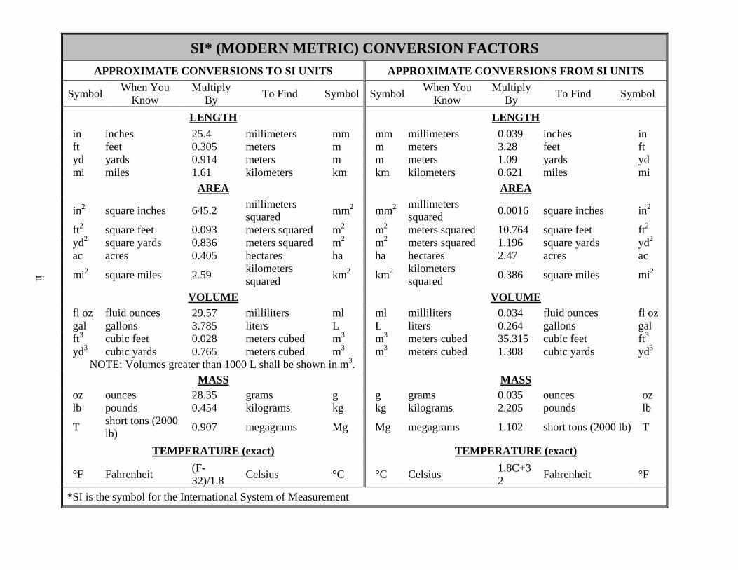
SI* (MODERN METRIC) CONVERSION FACTORS APPROXIMATE CONVERSIONS TO SI UNITS APPROXIMATE CONVERSIONS FROM SI UNITS

Symbol When You Know

Multiply By To Find Symbol Symbol When You

Know Multiply

By To Find Symbol

LENGTH LENGTH in inches 25.4 millimeters mm mm millimeters 0.039 inches in ft feet 0.305 meters m m meters 3.28 feet ft yd yards 0.914 meters m m meters 1.09 yards yd mi miles 1.61 kilometers km km kilometers 0.621 miles mi

AREA AREA

in2 square inches 645.2 millimeters squared mm2 mm2 millimeters

squared 0.0016 square inches in2

ft2 square feet 0.093 meters squared m2 m2 meters squared 10.764 square feet ft2 yd2 square yards 0.836 meters squared m2 m2 meters squared 1.196 square yards yd2 ac acres 0.405 hectares ha ha hectares 2.47 acres ac

mi2 square miles 2.59 kilometers squared km2 km2 kilometers

squared 0.386 square miles mi2

VOLUME VOLUME fl oz fluid ounces 29.57 milliliters ml ml milliliters 0.034 fluid ounces fl oz gal gallons 3.785 liters L L liters 0.264 gallons gal ft3 cubic feet 0.028 meters cubed m3 m3 meters cubed 35.315 cubic feet ft3 yd3 cubic yards 0.765 meters cubed m3 m3 meters cubed 1.308 cubic yards yd3

NOTE: Volumes greater than 1000 L shall be shown in m3. MASS MASS

oz ounces 28.35 grams g g grams 0.035 ounces oz lb pounds 0.454 kilograms kg kg kilograms 2.205 pounds lb

T short tons (2000 lb) 0.907 megagrams Mg Mg megagrams 1.102 short tons (2000 lb) T

TEMPERATURE (exact) TEMPERATURE (exact)

°F Fahrenheit (F-32)/1.8 Celsius °C °C Celsius 1.8C+3

2 Fahrenheit °F

*SI is the symbol for the International System of Measurement

iii

iv

ACKNOWLEDGEMENTS The author would like to thank the members of ODOT’s Technical Advisory Committee (William Fletcher, Mike Shippey, Alvin Shoblom, Cindy Callahan, Matthew Mabey, and Kira Glover-Cutter) as well as Elnaz Hassanpour, Zane Roberts, Gabriella Coughlin, Colleen Barr, Maoya Bassouni, and Robert Predosa for their invaluable help in the field, and fruitful discussions.

DISCLAIMER This document is disseminated under the sponsorship of the Oregon Department of Transportation and the United States Department of Transportation in the interest of information exchange. The State of Oregon and the United States Government assume no liability of its contents or use thereof. The contents of this report reflect the view of the authors who are solely responsible for the facts and accuracy of the material presented. The contents do not necessarily reflect the official views of the Oregon Department of Transportation or the United States Department of Transportation. The State of Oregon and the United States Government do not endorse products of manufacturers. Trademarks or manufacturers’ names appear herein only because they are considered essential to the object of this document. This report does not constitute a standard, specification, or regulation.

v

vi

DESIGN GUIDE FOR ROADSIDE INFILTRATION STRIPS IN WESTERN OREGON

TABLE OF CONTENTS

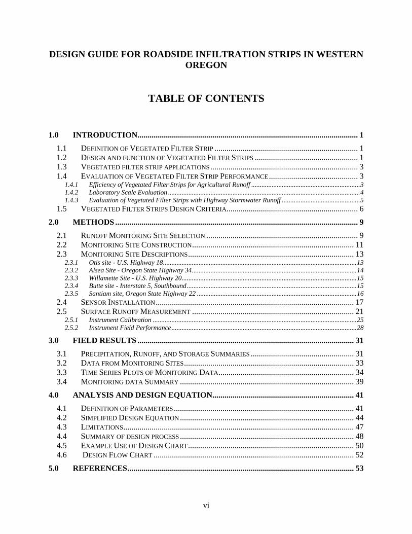
1.0 INTRODUCTION............................................................................................................. 1

1.1 DEFINITION OF VEGETATED FILTER STRIP ....................................................................... 1 1.2 DESIGN AND FUNCTION OF VEGETATED FILTER STRIPS ................................................... 1 1.3 VEGETATED FILTER STRIP APPLICATIONS ......................................................................... 3 1.4 EVALUATION OF VEGETATED FILTER STRIP PERFORMANCE ............................................ 3

1.4.1 Efficiency of Vegetated Filter Strips for Agricultural Runoff ................................................................ 3 1.4.2 Laboratory Scale Evaluation ................................................................................................................. 4 1.4.3 Evaluation of Vegetated Filter Strips with Highway Stormwater Runoff .............................................. 5

1.5 VEGETATED FILTER STRIPS DESIGN CRITERIA................................................................. 6

2.0 METHODS ........................................................................................................................ 9

2.1 RUNOFF MONITORING SITE SELECTION ........................................................................... 9 2.2 MONITORING SITE CONSTRUCTION ................................................................................ 11 2.3 MONITORING SITE DESCRIPTIONS .................................................................................. 13

2.3.1 Otis site - U.S. Highway 18 .................................................................................................................. 13 2.3.2 Alsea Site - Oregon State Highway 34 ................................................................................................. 14 2.3.3 Willamette Site - U.S. Highway 20 ....................................................................................................... 15 2.3.4 Butte site - Interstate 5, Southbound .................................................................................................... 15 2.3.5 Santiam site, Oregon State Highway 22 .............................................................................................. 16

2.4 SENSOR INSTALLATION .................................................................................................. 17 2.5 SURFACE RUNOFF MEASUREMENT ................................................................................ 21

2.5.1 Instrument Calibration ........................................................................................................................ 25 2.5.2 Instrument Field Performance ............................................................................................................. 28

3.0 FIELD RESULTS ........................................................................................................... 31

3.1 PRECIPITATION, RUNOFF, AND STORAGE SUMMARIES ................................................... 31 3.2 DATA FROM MONITORING SITES .................................................................................... 33 3.3 TIME SERIES PLOTS OF MONITORING DATA ................................................................... 34 3.4 MONITORING DATA SUMMARY ...................................................................................... 39

4.0 ANALYSIS AND DESIGN EQUATION...................................................................... 41

4.1 DEFINITION OF PARAMETERS ......................................................................................... 41 4.2 SIMPLIFIED DESIGN EQUATION ...................................................................................... 44 4.3 LIMITATIONS .................................................................................................................. 47 4.4 SUMMARY OF DESIGN PROCESS ...................................................................................... 48 4.5 EXAMPLE USE OF DESIGN CHART .................................................................................. 50 4.6 DESIGN FLOW CHART ................................................................................................... 52

5.0 REFERENCES ................................................................................................................ 53

vii

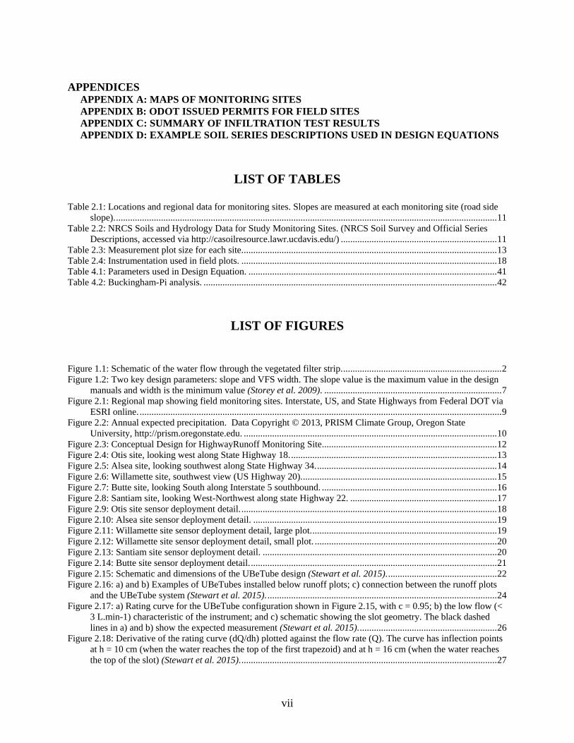
APPENDICES

APPENDIX A: MAPS OF MONITORING SITES APPENDIX B: ODOT ISSUED PERMITS FOR FIELD SITES APPENDIX C: SUMMARY OF INFILTRATION TEST RESULTS APPENDIX D: EXAMPLE SOIL SERIES DESCRIPTIONS USED IN DESIGN EQUATIONS

LIST OF TABLES

Table 2.1: Locations and regional data for monitoring sites. Slopes are measured at each monitoring site (road side slope). ................................................................................................................................................................. 11

Table 2.2: NRCS Soils and Hydrology Data for Study Monitoring Sites. (NRCS Soil Survey and Official Series Descriptions, accessed via http://casoilresource.lawr.ucdavis.edu/) .................................................................. 11

Table 2.3: Measurement plot size for each site. ........................................................................................................... 13 Table 2.4: Instrumentation used in field plots. ............................................................................................................ 18 Table 4.1: Parameters used in Design Equation. ......................................................................................................... 41 Table 4.2: Buckingham-Pi analysis. ............................................................................................................................ 42

LIST OF FIGURES

Figure 1.1: Schematic of the water flow through the vegetated filter strip. ................................................................... 2 Figure 1.2: Two key design parameters: slope and VFS width. The slope value is the maximum value in the design

manuals and width is the minimum value (Storey et al. 2009). ........................................................................... 7 Figure 2.1: Regional map showing field monitoring sites. Interstate, US, and State Highways from Federal DOT via

ESRI online. ......................................................................................................................................................... 9 Figure 2.2: Annual expected precipitation. Data Copyright © 2013, PRISM Climate Group, Oregon State

University, http://prism.oregonstate.edu. ........................................................................................................... 10 Figure 2.3: Conceptual Design for HighwayRunoff Monitoring Site .......................................................................... 12 Figure 2.4: Otis site, looking west along State Highway 18. ....................................................................................... 13 Figure 2.5: Alsea site, looking southwest along State Highway 34. ............................................................................ 14 Figure 2.6: Willamette site, southwest view (US Highway 20). .................................................................................. 15 Figure 2.7: Butte site, looking South along Interstate 5 southbound. .......................................................................... 16 Figure 2.8: Santiam site, looking West-Northwest along state Highway 22. .............................................................. 17 Figure 2.9: Otis site sensor deployment detail. ............................................................................................................ 18 Figure 2.10: Alsea site sensor deployment detail. ....................................................................................................... 19 Figure 2.11: Willamette site sensor deployment detail, large plot. .............................................................................. 19 Figure 2.12: Willamette site sensor deployment detail, small plot. ............................................................................. 20 Figure 2.13: Santiam site sensor deployment detail. ................................................................................................... 20 Figure 2.14: Butte site sensor deployment detail. ........................................................................................................ 21 Figure 2.15: Schematic and dimensions of the UBeTube design (Stewart et al. 2015). .............................................. 22 Figure 2.16: a) and b) Examples of UBeTubes installed below runoff plots; c) connection between the runoff plots

and the UBeTube system (Stewart et al. 2015). ................................................................................................. 24 Figure 2.17: a) Rating curve for the UBeTube configuration shown in Figure 2.15, with c = 0.95; b) the low flow (<

3 L.min-1) characteristic of the instrument; and c) schematic showing the slot geometry. The black dashed lines in a) and b) show the expected measurement (Stewart et al. 2015). .......................................................... 26

Figure 2.18: Derivative of the rating curve (dQ/dh) plotted against the flow rate (Q). The curve has inflection points at h = 10 cm (when the water reaches the top of the first trapezoid) and at h = 16 cm (when the water reaches the top of the slot) (Stewart et al. 2015). ............................................................................................................ 27

viii

Figure 2.19: Results of laboratory validation experiment. Uncorrected measurements are represented by gray-filled circles while the measurements corrected using Equation 2-4 are represented by the open diamonds. Each point represents the mean flow rate (Stewart et al. 2015). ................................................................................. 28

Figure 2.20: Examples of field applications of the UBeTube instrument in a long-term study measuring highway stormwater runoff produced by highway surfaces within western Oregon. Data comes from a) Otis and b) Santiam sites. The left y-axis shows the runoff rate by the instrument and the right y-axis shows the natural rainfall as measured by tipping bucket rain gauges installed at the sites (Stewart et al. 2015). ......................... 29

Figure 3.1: Measured Wet season precipitation total. Measurement period Oct 1-May3. Willamette data is for 3 m plot. .................................................................................................................................................................... 31

Figure 3.2: Measured total runoff and change in water stored within the infiltration strip. Measurement period Oct.1 - May 31. Willamette data is from the 3m plot. ................................................................................................. 32

Figure 3.3: Rainfall, runoff and soil moisture time series at the Alsea site. D represents depth and L length for Figures 3.3-3.7. .................................................................................................................................................. 34

Figure 3.4: Rainfall, runoff and soil moisture time series at the Santiam site. ............................................................ 35 Figure 3.5: Rainfall, runoff and soil moisture time series at the small Willamette site, 3m (10 ft). ............................ 36 Figure 3.6: Rainfall, runoff and soil moisture time series at the Butte site. ................................................................. 37 Figure 3.7: Rainfall, runoff and soil moisture time series at the Otis site. ................................................................... 38 Figure 3.8: Synthesized site data for the entire project. Rainfall and runoff values are totals for the season. ............ 40 Figure 4.1: The relationship between the SSURGO values of saturated conductivity and the slope of the saturation

curve multiplied by the profile depth. R2 = 0.87. ............................................................................................... 44 Figure 4.2: Relationships between dimensionless groups. Increased slopes are correlated to decreased infiltration,

Increased rate of recession with increased infiltration, and increased precipitation with decreased infiltration. ........................................................................................................................................................................... 45

Figure 4.3: The collapsed data: Data taken over the rainy season during the two year study have collapsed into a single relationship that can be fit to a function. This fitted function is the design equation (MATLAB) R2 = 0.73. ................................................................................................................................................................... 46

Figure 4.4: Design chart for roadside infiltration strips. Each line corresponds to soil, slope and precipitation characteristics unique to potential sites. ............................................................................................................. 47

Figure 4.5: Example use of design chart. ..................................................................................................................... 51 Figure 4.6: Design flow chart ...................................................................................................................................... 52

ix

x

EXECUTIVE SUMMARY Roadside infiltration strips, also called vegetated filter strips, have the ability to decrease the immediate impact of road runoff on nearby streams and agricultural fields. Though there is a rich history of research on the chemical and physical filtering capabilities of these structures, total infiltration capacity is often not the focus of these research efforts. By using dimensional analysis of a varied infiltration capacity dataset, this research developed a new design equation and subsequent design chart to simplify and streamline the infiltration strip design process. Given that the parameters and variables used in this design process are freely available in map form, a preliminary analysis of all roads within the western corridor of Oregon could be performed in GIS for future filter width design. The design equation was created by the following process. 1) A network of roadside infiltration observation plots was constructed and operated for 2 years. The network consisted of five plots arranged in a transect from the Oregon coast to the Cascade foothills. Within each plot, rainfall, soil moisture, soil water content and total runoff from the observation area were recorded every 15 minutes and averaged into daily infiltration intervals; 2) Semi-empirical relationships between the road geometry, the soil physical properties, and the local climate were explored with dimensional analysis; 3) Final groupings of variables were found, collapsing the data to a single semi-empirical relationship. This relationship is the design equation. For practical design applications, a specified range of variables was used to turn the design equation into a design chart. This report is divided into 4 sections. An introduction and general background is presented in Section 1, followed by a detailed description of each study sited is presented in Section 2. In Section 3, summary statistics and time series of the data are presented. In Section 4, the rationale and logical process to create the design equation is outlined, and the ultimate design equation and design chart is given. The report is concluded with an example calculation of a roadside filter strip width.

xi

1

1.0 INTRODUCTION

1.1 DEFINITION OF VEGETATED FILTER STRIP

Vegetated filter strips (VFS) are areas of land designed to receive surface runoff water as overland sheet flow. Ideally these are designed with mild slopes (2%-6%), high soil infiltration rates, and dense grassy vegetation. Surface vegetation decreases runoff flow velocities, allowing infiltration and filtration of sediments and other pollutants (Dillaha et al. 1989). VFS can potentially protect nearby water bodies through the following (Grismer 2006):

• Surface runoff interception and sediment entrapment (75-100% infiltration has been reported);

• Nutrient removal from runoff water, both through soil adsorption or plant root uptake;

• Reduction of transport of pollutants (including heavy metals) increasing their degradation;

• Pathogen removal from the runoff water.

There are generally four categories of VFS (Dosskey et al. 2007):

• Constructed VFS: filter strips that are constructed and maintained for overland sheet flow through the surface vegetation;

• Natural VFS: any natural vegetative area through which stormwater flow is directed. Flow is typically broad overland sheet flow;

• Riparian vegetated buffer strip: strips of vegetation that grow along the stream and concentrated flow channels;

• Adjacent to agricultural lands, providing a buffer against excess nutrient-laden runoff where applicable.

1.2 DESIGN AND FUNCTION OF VEGETATED FILTER STRIPS

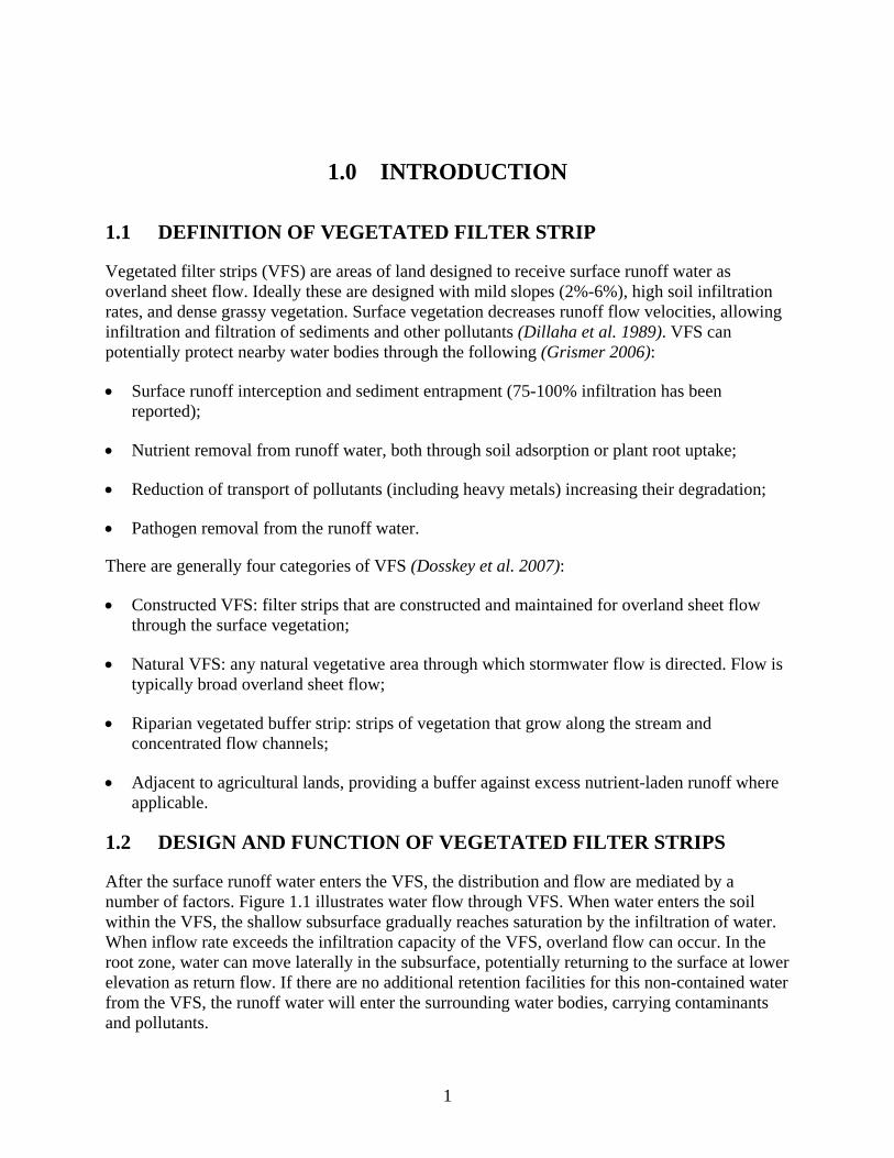
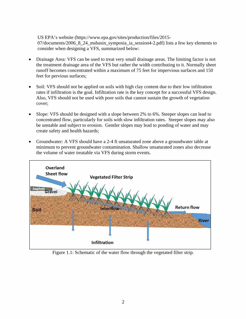
After the surface runoff water enters the VFS, the distribution and flow are mediated by a number of factors. Figure 1.1 illustrates water flow through VFS. When water enters the soil within the VFS, the shallow subsurface gradually reaches saturation by the infiltration of water. When inflow rate exceeds the infiltration capacity of the VFS, overland flow can occur. In the root zone, water can move laterally in the subsurface, potentially returning to the surface at lower elevation as return flow. If there are no additional retention facilities for this non-contained water from the VFS, the runoff water will enter the surrounding water bodies, carrying contaminants and pollutants.

2

US EPA’s website (https://www.epa.gov/sites/production/files/2015-07/documents/2006_8_24_msbasin_symposia_ia_session4-2.pdf) lists a few key elements to consider when designing a VFS, summarized below:

• Drainage Area: VFS can be used to treat very small drainage areas. The limiting factor is not the treatment drainage area of the VFS but rather the width contributing to it. Normally sheet runoff becomes concentrated within a maximum of 75 feet for impervious surfaces and 150 feet for pervious surfaces;

• Soil: VFS should not be applied on soils with high clay content due to their low infiltration rates if infiltration is the goal. Infiltration rate is the key concept for a successful VFS design. Also, VFS should not be used with poor soils that cannot sustain the growth of vegetation cover;

• Slope: VFS should be designed with a slope between 2% to 6%. Steeper slopes can lead to concentrated flow, particularly for soils with slow infiltration rates. Steeper slopes may also be unstable and subject to erosion. Gentler slopes may lead to ponding of water and may create safety and health hazards;

• Groundwater: A VFS should have a 2-4 ft unsaturated zone above a groundwater table at minimum to prevent groundwater contamination. Shallow unsaturated zones also decrease the volume of water treatable via VFS during storm events.

Figure 1.1: Schematic of the water flow through the vegetated filter strip.

3

1.3 VEGETATED FILTER STRIP APPLICATIONS

Because VFS are an efficient and cost-effective runoff treatment method, VFS have been used to control surface runoff under many situations. VFS have been primarily utilized at the boundaries of agricultural fields, next to impervious surfaces like roadways, and adjacent to water bodies as riparian buffers. In all instances, VFS are installed with the goal of slowing, filtering, and capturing nutrient- and pollutant-laden runoff through infiltration into the soil, filtration of flow by the vegetation, plant uptake, transpiration, and other biologically active components. Much of the work has focused on the ability of VFS to remove specific chemicals, including agricultural pesticides (Poletika et al. 2009; Fox et al. 2011) and herbicides (Arora et al. 1996) and in the case of roadside buffers, heavy metals (Stagge et al. 2012) and suspended solids (Stagge et al. 2012). Recent review papers have focused on nitrogen (USEPA 2005; Mayer et al. 2007), phosphorous (Hoffmann et al. 2009) and suspended sediment (Liu et al. 2008; Yuan et al. 2009). VFS can provide various levels of treatment for the target pollutants based on their size, slope, vegetation type, and climate conditions.

Vegetated Filter Strips (VFS) are also used to reduce peak runoff rates, filter and adsorb pollutants and nutrients, and mitigate flooding. VFS have been previously utilized to remove sediment (Dosskey et al. 2008), colloids (defined as particles smaller than 10 μm in diameter) (Yu et al. 2011; Yu et al. 2012; Yu et al. 2013), and solutes (Fischer and Fischenich 2000; Gao et al. 2005; Dosskey et al. 2007; Dosskey et al. 2008; Muñoz-Carpena et al. 2010; Fox et al. 2011) that are carried in runoff water. Riparian buffers are a special type of VFS which, due to their proximity to water bodies, have been extensively studied (USEPA 2005; Mayer et al. 2007; Dosskey et al. 2008). Koelsch, Lorimer et al. (Koelsche, Lorimer et al. 2006) reviewed the literature with the goal of understanding how VFS could be used in conjunction with concentrated animal feeding operations.

1.4 EVALUATION OF VEGETATED FILTER STRIP PERFORMANCE

Due to the widespread implementation of VFS, extensive work has been done to evaluate the performance of VFS in different environments. To evaluate the performance of VFS, either field scale monitoring or laboratory scale experiment can be conducted to collect data. Given adequate validation, numerical modeling can be used to understand and predict the performance of VFS under different scenarios and more extensive scales. When evaluating the performance of a VFS, there are two fundamental aspects to examine: pollutant removal efficiency and runoff volume reduction efficiency. We reviewed previous studies which fell into the three broad categories: agricultural runoff; laboratory evaluations; and highway stormwater runoff.

1.4.1 Efficiency of Vegetated Filter Strips for Agricultural Runoff

Agricultural runoff usually contains significant amounts of nutrients (nitrogen and phosphorous), sediments, herbicides, and pesticides. VFS is very suitable in reducing these nonpoint source pollutants. For nutrients coming from feedlots, Young et al. (Young et al. 1980) studied a 13.7 m VFS with 4% slope and found the removal efficiency for phosphorous and nitrogen can reach 88% and 87%. Similarly, Doyle et al. (Doyle et al. 1977), Dilaha et al. (Dilaha et al. 1988), Moore et al. (Moore et al. 2001) all found that VFS can be very efficient in reducing the concentrations of nutrients in feedlot runoff.

4

For cropland runoff, Cole et al. (Cole et al. 1997) investigated the removal efficiency of Bermuda grass-covered buffer strip for four pesticides and found for a 4.8 m plot width, the average removal rate for all four target pesticides exceeds 80%. For a similar plot width, Parsons et al. (Parsons et al. 1991) and Barfield et al. (Barfield et al. 1992) showed that VFS removed 50% total N and 92% NH4-N, respectively. In another study, the total solids and total suspended solid removal rate by VFS can be as high as 100% (Patty et al. 1997).

Some research has studied the effect of VFS width on the nutrient removal efficiency (Dillaha et al. 1989; Schmitt et al. 1999; Blanco-Canqui et al. 2004). VFS width is an important variable affecting the efficacy of a VFS. The runoff water will have a longer time to interact with the soil in VFS if it has a greater width. Longer retention time means more infiltration. Dillaha et al. (Dillaha et al. 1989) reported that when the VFS plot width was doubled from 4.6 m to 9.1 m, the removal efficiency for total phosphorous was increased from 75% to 87%, however the total nitrogen removal efficiency was not changed. Blanco-Canqui et al. (Blanco-Canqui et al. 2004) stated in their study that the effectiveness of the grass treatment for reducing sediment and nutrient loss increased with the VFS width, but the reductions beyond 4 m were small. Similarly, Schmitt et al. (Schmitt et al. 1999) found that doubling the VFS with from 7.5m to 15m would significantly increase infiltration and dilution of runoff, but did little to improve sediment entrapment.

1.4.2 Laboratory Scale Evaluation

The efficiency of VFS can be evaluated under laboratory environments. The advantage of conducting laboratory study is that environmental variables can be controlled. Further, experiments can be repeated to acquire reproducible results. Under field conditions, especially for long-term monitoring, it is very difficult to repeat measurements under similar conditions.

Huang et al. (Huang et al. 2013) studied the effect of rainfall intensity, slope, initial soil moisture content, and vegetation cover on runoff intensity. In this study, an adjustable soil bed was used to simulate a vegetated soil slope and rainfall was simulated by using sprinklers. They found a positive linear relationship between runoff intensity and the rainfall intensity, slope, and initial soil water content. Also a negative relationship was found between runoff rate and vegetation cover.

Similar to Huang’s experimental setup, Newberry and Yonge (Newberry and Yonge 1996) employed a 1.2 m wide and 3 m long flow bed to determine the effectiveness of the VFS as a retention mechanism. Simulated rainfall was used with spiked pollutants in the water. For different flow and slope combinations, the hydraulic retention time was reported from 8.8 min at a flow of 3.8 L/min and 17% slope to 85.3 min for 0.38 L/min flow with a slope of 5%. The VFS in this study also demonstrated very good heavy metal retention rate within the first 1 m.

The hydraulic and pollutant removal performance of VFS was studied using soil columns (Hatt et al. 2008). A 10 cm diameter and 1 m long pipe was used to represent a vertical soil profile, and they found that clogging at the top layer can lead to hydraulic failure. Although the sediments and heavy metals were retained effectively by the soil filter, nitrogen and phosphorus can be released from the soil.

5

Laboratory experiments can provide valuable information for evaluating the efficiency of VFS. However, it is difficult to scale up results to field conditions due to the complexity and variability in the natural environment. Piguet et al. (Piguet et al. 2008) made the effort to carry a real-scale experiment and they used field lysimeters for infiltration measurement. This study can be considered more like a field-scale experiment, especially with the natural rainfall events used. The results show that the infiltration system is efficient at retaining pollutants with low mobility in the soil, whereas highly mobile pollutants can percolate through the infiltration system during intensive rainfall events.

1.4.3 Evaluation of Vegetated Filter Strips with Highway Stormwater Runoff

Stormwater runoff from road surfaces has been identified as a major potential pollutant source which greatly affects water quality (USEPA 2005). Stormwater contains a variety of pollutants including heavy metals, sediments, nutrients, and hydrocarbons (Kayhanian et al. 2007; Diblasi et al. 2009). VFS has been employed to remove pollutants and reduce peakflow due to its advantages in a highway setting. Therefore, it is necessary to evaluate the efficacy of the existing VFS under a natural environment. For an effort like this, especially for field conditions, it normally requires the installation of a monitoring plot on the slope of the VFS. Most field studies of VFS performance require a means to collect and/or measure the runoff which occurs at the downhill edge of the VFS. Runoff measurement strategies have included collecting water in large tanks (Arora et al. 1996), passing water through roadside weir (Winston et al. 2011) or tipping bucket (Hollis and Ovenden 1987) systems to measure the discharge rates. Collecting water in a tank allows for easy collection of water samples to determine chemistry and concentration of the studied constituents, though any sample will be an average of all collected water in the tank, which may obfuscate temporal trends in chemistry. Further, using collection tanks in long-term studies necessitates periodic emptying and maintenance to ensure that the tanks do not fully fill. The weir and tipping bucket systems are conducive to long-term monitoring of runoff quantities, as they do not retain water but rather measure discharge in real time.

Line and Hunt (Line and Hunt 2009) evaluated the performance of a level grass filter strip in North Carolina. Inflow and outflow for the VFS were monitored for 13 storm events. The results were compared with a bioretention area and showed that VFS had the best overall efficiency in all target pollutants. The inflow volume and peak flow rate were reduced by 49% and 23%, respectively.

In another study, also carried in North Carolina (Winston et al. 2012), the existing VFS along the highway roadside were tested for pollutant removal efficiency with traditional dry swales and wetland swales. The two testing sites in this study had steep slopes of 18.1% and 15.8%. These high slopes were reported to be responsible for significant increase in total phosphorus and total suspended solids (TSS) concentration from the edge of the pavement. High inflow pollutant concentration and ground cover percentage were also related to this observation. They also found that the efficiency of the VFS were not as high as expected because of the soil compaction (less infiltration) on the highway shoulder.

A third North Carolina based study investigated the capacity of VFS in carbon (C) sequestration (Bouchard et al. 2013). Soil core samples were taken from an existing highway VFS to look for

6

soil carbon content. This was a pioneering work to look into the C sequestration in roadway soils. The reported data indicates that roadside VFS is a potential source or sink to be accounted for in global C stock quantification.

Stagge et al. (Stagge et al. 2012) reported a 4.5 year long-term field monitoring in Maryland. The performance of grass swales and VFS were evaluated over 45 storm events. Interestingly, while the grass swale reduced the pollutant mass and mean concentration significantly, the inclusion of the pre-treatment vegetated filter strip produced mostly negligible improvement with respect to water quality. The hydraulic performance of the VFS was also examined by the same research team (Davis et al. 2012), and the grass swale significantly reduced runoff volume and flow magnitude with small rainfall events (< 3cm). For large rainfall events the grass showed very limited capacity in runoff volume reduction. The inclusion of VFS in terms of reducing runoff volume produced mixed effects in this study.

There are many research reports also related to the evaluation of the efficiency of the VFS in highway applications. Some intensive studies from Washington State can be found in Reister and Fiedler (Reister and Fiedler 2006), Horner et al. (Horner et al. 2002), Reister and Yonge (Reister and Yonge 2005), Newberry and Yonge (Newberry and Yonge 1996), Ahearn and Tveten (Ahearn and Tveten 2008). With the rapid acceptance of the Low Impact Development (LID) concept in the literature, the evaluation of LID efficiency is what ensures its performance. VFS is a particularly appropriate LID practice in highway settings due to the linear nature of the right-of-way and the limited space for stormwater treatment facilities. Ahearn and Tveten (Ahearn and Tveten 2008) studied the efficiency of unimproved highway VFS in stormwater runoff treatment. By using 2 m and 4 m width monitoring plots installed at edge of the pavement, they reported that 79% of the runoff volume was infiltrated with in the first 2 m of VFS and 83% was infiltrated within 4 m. Peak flow rates were reduced by 72% and 90% at 2 m and 4 m, respectively.

Reister and Yonge (Reister and Yonge 2005), and Reister and Fiedler (Reister and Fiedler 2006) used field data and numerical modelling to investigate the effects of rainfall intensity, roadway width, plot width, soil properties, and slope on VFS efficiency. By combining field data from 2 m and 4 m wide plots with numerical modeling, they determined a site-specific relationship between VFS width, roadway width, soil saturated hydraulic conductivity and rainfall intensity. What is worth mentioning was the effect of slope angle on runoff was not correlated by experimental data or numerical modeling, whereas slope was an important factor to consider when designing capable VFS (that is, VFS systems capable of reducing runoff by a significant amount).

1.5 VEGETATED FILTER STRIPS DESIGN CRITERIA

So far many state agencies have made the effort to produce a design manual for various types of stormwater BMPs as well as certain evaluation criteria to determine the VFS efficiency. In general, such design manuals and performance reports can be found on state DOT’s database and they are available to public.

7

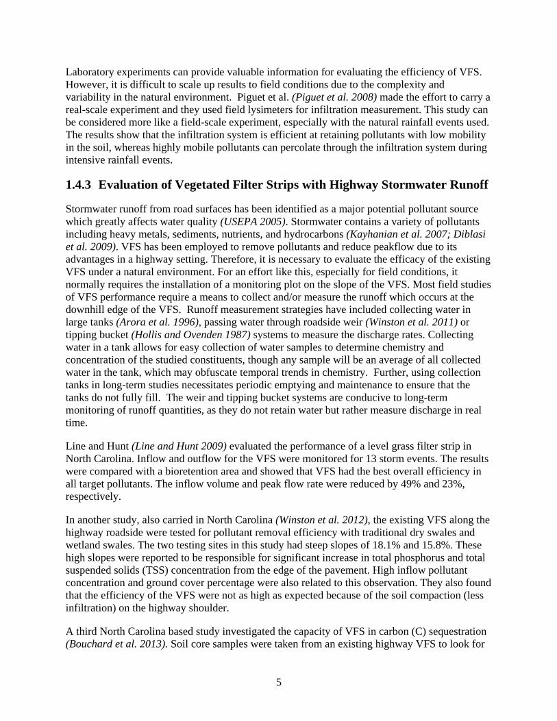
The Texas Transportation Institute (Storey et al. 2009) synthesized Best Management Practices by multiple transportation, environmental, and regulatory agencies regarding the use of vegetated buffer strips, filter strips, and grass swales. Readers are referred to Appendix A in Storey’s report for detailed information. Note that among these design manuals, the key parameters can vary substantially. Figure 1.2 shows typical slope and width used in VFS designs.

High variation and accumulation of annual rainfall together with unique soil classifications, such as the heavy soils of the Willamette valley associated with the Missoula floods, present a unique VFS design challenge for Oregon. Despite the amount of work that has been done in design and

evaluation of VFS, existing studies are not directly useful when developing regionally specific design guidelines for highways in western Oregon. Typically, there is no regulatory requirement to monitor BMP performance, and long term data is not collected in these cases. In most of the literature, water quality measures from the perspective of contaminant removal are considered as opposed to runoff quantity (infiltration).

Figure 1.2: Two key design parameters: slope and VFS width. The slope value is the

maximum value in the design manuals and width is the minimum value (Storey et al. 2009).

Wid

th

8

This report endeavors to forge a new path for VFS design guidance when infiltration/runoff reduction is the primary goal. The approach is based on dimensional analysis of two years of field measurements that span a wide range of soil characteristics and climates representative of western Oregon in order to synthesize a design equation that can guide VFS width selection along highways. Specifically, the research strategy was to generate regional data guided by the range of conditions likely to be encountered throughout this region. First, considering the total annual precipitation from the coast to the Cascades varies from less than 40” to over 100”, monitoring locations were selected to represent this variability. Second, given the large diversity of Oregon soils, each monitoring location was selected to cover a wide range of hydrologic characteristics that influence infiltration rates such as soil texture, hydraulic conductivity, and drainage class. In sum, over two years of data was collected from five distinct sites from the coast to the Cascades to develop VFS design criteria for the expected range of conditions that can be encountered across western Oregon.

9

2.0 METHODS

2.1 RUNOFF MONITORING SITE SELECTION

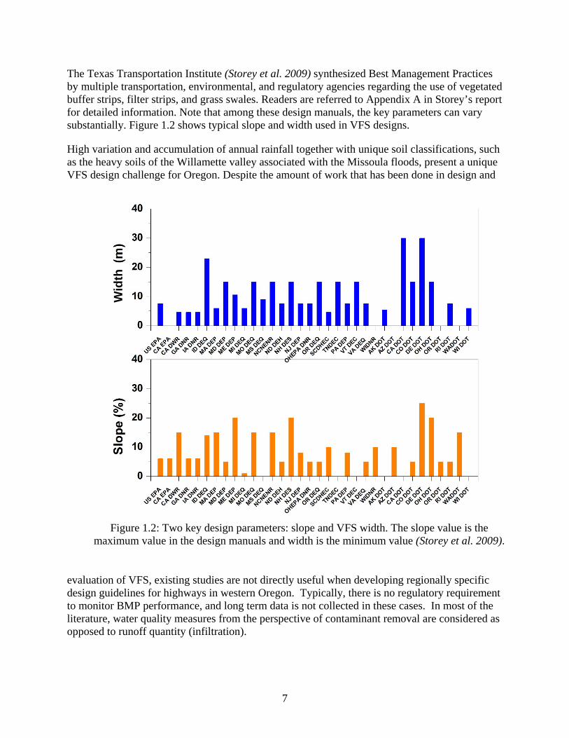
Runoff is primarily controlled by the amount of precipitation received and the infiltration capacity of the underlying soil strata. Five field scale monitoring sites were constructed and maintained for two years to evaluate the stormwater runoff from the highway road surface under natural precipitation conditions (Figure 2.1). These sites were selected to represent the full range of combinations of precipitation and infiltration possible in western Oregon. The first criteria for site selection was to represent the full range of precipitation in western Oregon, which varies from 40-50 inches annually in the Willamette valley to over 100” received annually in some parts of the Coast Range (Figure 2.2). Sites were also selected to represent a broad range of soil types, soil hydrology, and road side slope, all of which control the rate, volumetric capacity, and seasonality of infiltration. Initially, over 10 sites were identified that fulfilled these basic criteria. Site selection also considered minimizing maintenance and travel costs, worker safety, and road geometry. Final decisions were made in negotiation with Oregon DOT staff. Five sites were

Figure 2.1: Regional map showing field monitoring sites. Interstate, US, and State Highways from

Federal DOT via ESRI online.

10

selected that fulfilled all the study design requirements (Figure 2.1 and Table 2.1).

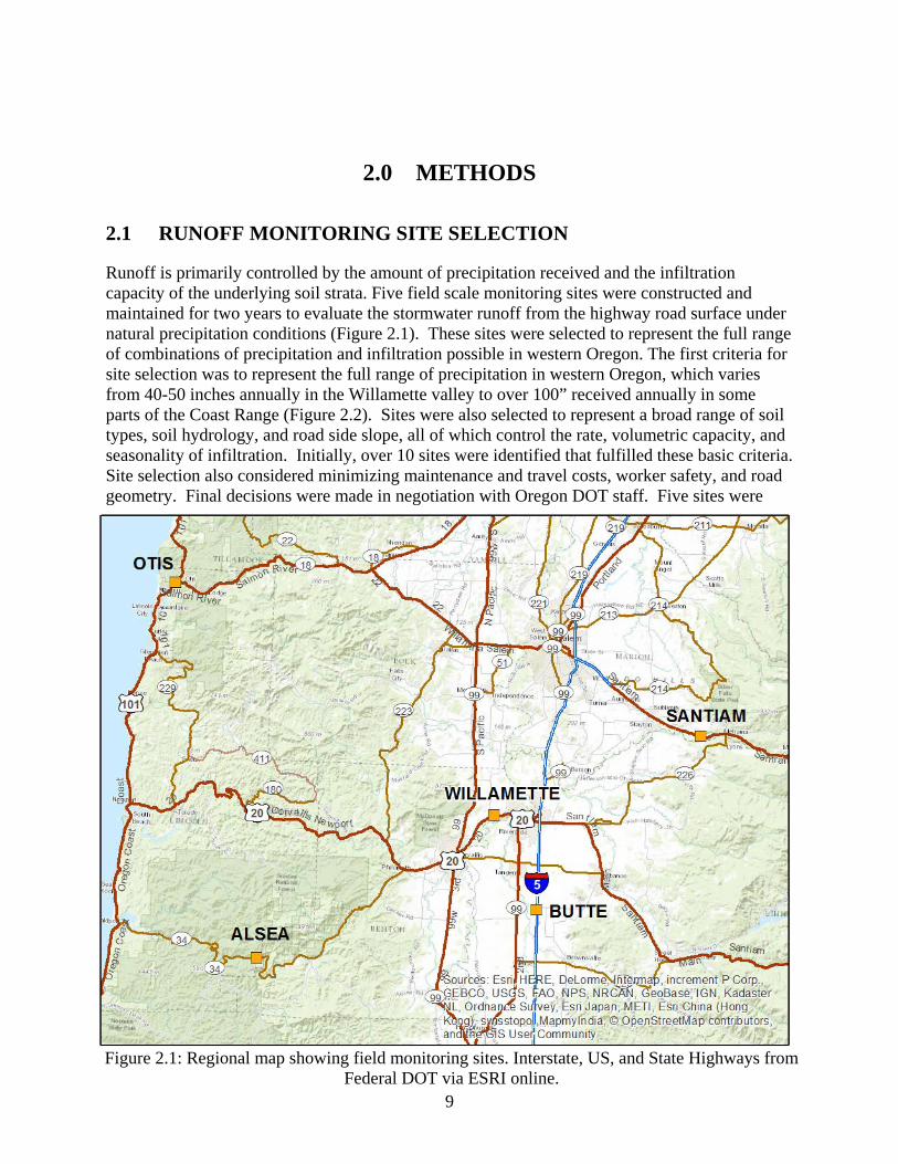
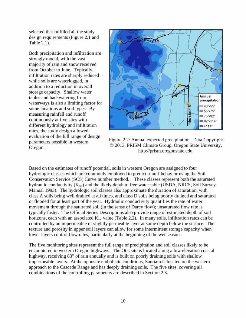
Both precipitation and infiltration are strongly modal, with the vast majority of rain and snow received from October to June. Typically, infiltration rates are sharply reduced while soils are waterlogged, in addition to a reduction in overall storage capacity. Shallow water tables and backwatering from waterways is also a limiting factor for some locations and soil types. By measuring rainfall and runoff continuously at five sites with different hydrology and infiltration rates, the study design allowed evaluation of the full range of design parameters possible in western Oregon.

Based on the estimates of runoff potential, soils in western Oregon are assigned to four hydrologic classes which are commonly employed to predict runoff behavior using the Soil Conservation Service (SCS) Curve number method. These classes represent both the saturated hydraulic conductivity (Ksat) and the likely depth to free water table (USDA, NRCS, Soil Survey Manual 1993). The hydrologic soil classes also approximate the duration of saturation, with class A soils being well drained at all times, and class D soils being poorly drained and saturated or flooded for at least part of the year. Hydraulic conductivity quantifies the rate of water movement through the saturated soil (in the sense of Darcy flow); unsaturated flow rate is typically faster. The Official Series Descriptions also provide range of estimated depth of soil horizons, each with an associated Ksat value (Table 2.2). In many soils, infiltration rates can be controlled by an impermeable or slightly permeable layer at some depth below the surface. The texture and porosity in upper soil layers can allow for some intermittent storage capacity when lower layers control flow rates, particularly at the beginning of the wet season.

The five monitoring sites represent the full range of precipitation and soil classes likely to be encountered in western Oregon highways. The Otis site is located along a low elevation coastal highway, receiving 83” of rain annually and is built on poorly draining soils with shallow impermeable layers. At the opposite end of site conditions, Santiam is located on the western approach to the Cascade Range and has deeply draining soils. The five sites, covering all combinations of the controlling parameters are described in Section 2.3.

Figure 2.2: Annual expected precipitation. Data Copyright © 2013, PRISM Climate Group, Oregon State University,

http://prism.oregonstate.edu.

11

Table 2.1: Locations and regional data for monitoring sites. Slopes are measured at each monitoring site (road side slope).

Road/Site Latitude Longitude Elevation (feet) Slope

Road Width (feet)

30-yr Average Precipitation (millimeters)

30-yr Average Precipitation

(inches) Highway 34 / Alsea 44.38 N 123.73 W 174 8% 24 1796 71

Highway 22 / Santiam 44.79 N 122.68 W 577 8% 67 1540 61

Highway 18 / Otis 45.02 N 123.97 W 19 10% 32 2099 83

Interstate 5 S.B. / Butte 44.48 N 123.06 W 258 13% 24 1076 42

Highway 20 / Willamette 44.64 N 123.17 W 208 4% 24 1093 43

Highway 20 / Willamette 44.64 N 123.17 W 208 4% 24 1093 43

Table 2.2: NRCS Soils and Hydrology Data for Study Monitoring Sites. (NRCS Soil Survey and Official Series Descriptions, accessed via http://casoilresource.lawr.ucdavis.edu/)

Road Number / Site

NRCS Soil Classification

(SSURGO)

NRCS Hydrologi

c Soil Class

Depth to impermeable layer

or typical water table depth

Ksat [shallowdeep]

(mm/hr)

Ksat [shallowdeep]

(in/hr)

Highway 34 / Alsea Nehalem SiL B Very deep, well

drained 32.4 1.25

Highway 22 / Santiam

Cloquato SiL; Camas Gr. SL

B; A

Very deep, well drained; excessively

drained

[32 101]; [101 1080]

[1.25 4.0]; [4.0 42]

Highway 18 / Otis

Coquille SiL; Chitwood SiL

C/D; C

4-7” (100-175mm); 7-20” (175-500mm)

[32 3]; [1343 3]

[1.25 4.0]; [4.0 42]

Interstate 5 S.B. / Butte Bashaw SiC D 3-10” (75-250mm) 0.7 0.03

Highway 20 / Willamette Malabon SiCL C Very deep, well

drained [32 10 32] [1.25 0.4 1.25]

2.2 MONITORING SITE CONSTRUCTION

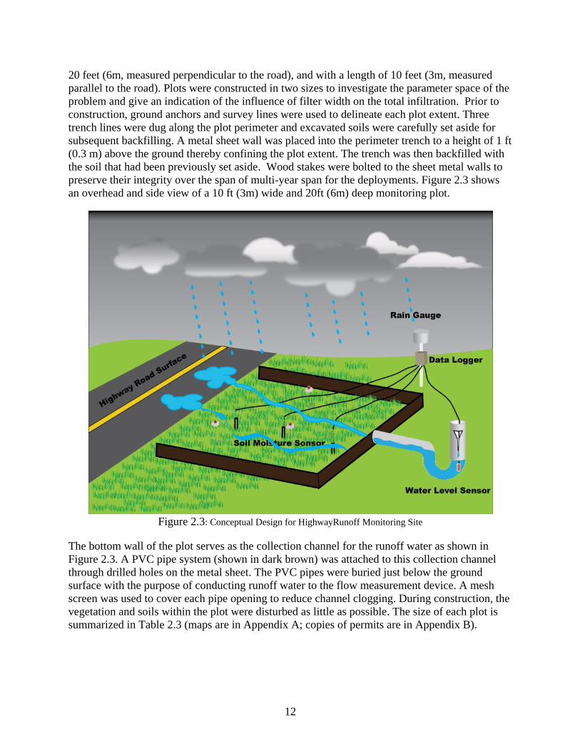
We designed and constructed five roadside runoff monitoring sites for an intensive field campaign. The sites were chosen to capture a range in variability of precipitation, soil type and highway shoulder slope. A schematic illustrating the conceptual design is shown in Figure 2.3. The experimental setup was designed to quantitatively capture parameters that constrain surface runoff as a function of precipitation rate within a confined vegetated area adjacent to the road surface. As runoff water flows over the vegetated filter strip, percolation data is captured and measured at instrumented distances from the road edge so that the vegetated filter strip width that is needed to absorb overland flow can be evaluated.

The uphill edge of each runoff plot corresponded to the outer edge of the roadside gravel strip (where vegetation begins). This roadside edge of each plot was left undisturbed throughout the campaign. Each plot was built with a width (distance from gravel edge) of either 10 feet (3m) or

12

20 feet (6m, measured perpendicular to the road), and with a length of 10 feet (3m, measured parallel to the road). Plots were constructed in two sizes to investigate the parameter space of the problem and give an indication of the influence of filter width on the total infiltration. Prior to construction, ground anchors and survey lines were used to delineate each plot extent. Three trench lines were dug along the plot perimeter and excavated soils were carefully set aside for subsequent backfilling. A metal sheet wall was placed into the perimeter trench to a height of 1 ft (0.3 m) above the ground thereby confining the plot extent. The trench was then backfilled with the soil that had been previously set aside. Wood stakes were bolted to the sheet metal walls to preserve their integrity over the span of multi-year span for the deployments. Figure 2.3 shows an overhead and side view of a 10 ft (3m) wide and 20ft (6m) deep monitoring plot.

Figure 2.3: Conceptual Design for HighwayRunoff Monitoring Site

The bottom wall of the plot serves as the collection channel for the runoff water as shown in Figure 2.3. A PVC pipe system (shown in dark brown) was attached to this collection channel through drilled holes on the metal sheet. The PVC pipes were buried just below the ground surface with the purpose of conducting runoff water to the flow measurement device. A mesh screen was used to cover each pipe opening to reduce channel clogging. During construction, the vegetation and soils within the plot were disturbed as little as possible. The size of each plot is summarized in Table 2.3 (maps are in Appendix A; copies of permits are in Appendix B).

13

Table 2.3: Measurement plot size for each site.

2.3 MONITORING SITE DESCRIPTIONS

Site maps showing site locations, slopes and soil classifications can be found in Appendix A.

Official Soil Series Descriptions can be found in Appendix D.

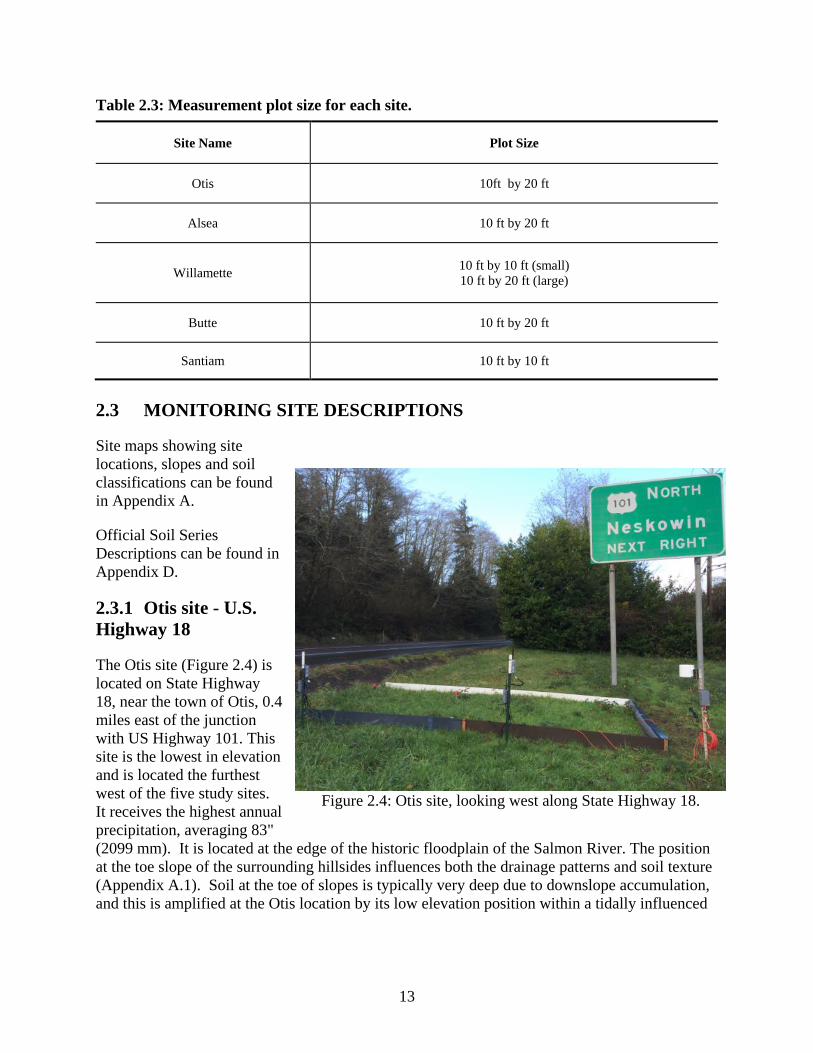
2.3.1 Otis site - U.S. Highway 18

The Otis site (Figure 2.4) is located on State Highway 18, near the town of Otis, 0.4 miles east of the junction with US Highway 101. This site is the lowest in elevation and is located the furthest west of the five study sites. It receives the highest annual precipitation, averaging 83" (2099 mm). It is located at the edge of the historic floodplain of the Salmon River. The position at the toe slope of the surrounding hillsides influences both the drainage patterns and soil texture (Appendix A.1). Soil at the toe of slopes is typically very deep due to downslope accumulation, and this is amplified at the Otis location by its low elevation position within a tidally influenced

Site Name Plot Size

Otis 10ft by 20 ft

Alsea 10 ft by 20 ft

Willamette 10 ft by 10 ft (small) 10 ft by 20 ft (large)

Butte 10 ft by 20 ft

Santiam 10 ft by 10 ft

Figure 2.4: Otis site, looking west along State Highway 18.

14

floodplain. Subsurface flows tend to accumulate at concave contours (NRCS Soil Survey Manual, Figure 3.1). The Otis site position on a convex radial convex contour indicates a shallow water table is unlikely.

The soil profile at the OTIS site is consistent with its location in the landscape (Appendix A.2). From the Official Series Descriptions: "The Chitwood series consists of very deep, somewhat poorly drained soils on coastal marine and valley terraces. They formed in alluvium derived from sedimentary rocks. Slopes range from 0 to 15 percent." Directly north of Highway 18 (towards the Salmon River), the soil is mixed alluvium: "The Coquille series consists of very deep, very poorly drained soils that formed in mixed alluvium along tidal influenced flood plains. Slopes are 0 to 1 percent." High local relief, the elevated position above the floodplain terrace, and deep soil profile indicate that soil water storage potential is high, despite the poorly drained soils (Appendix A.2).

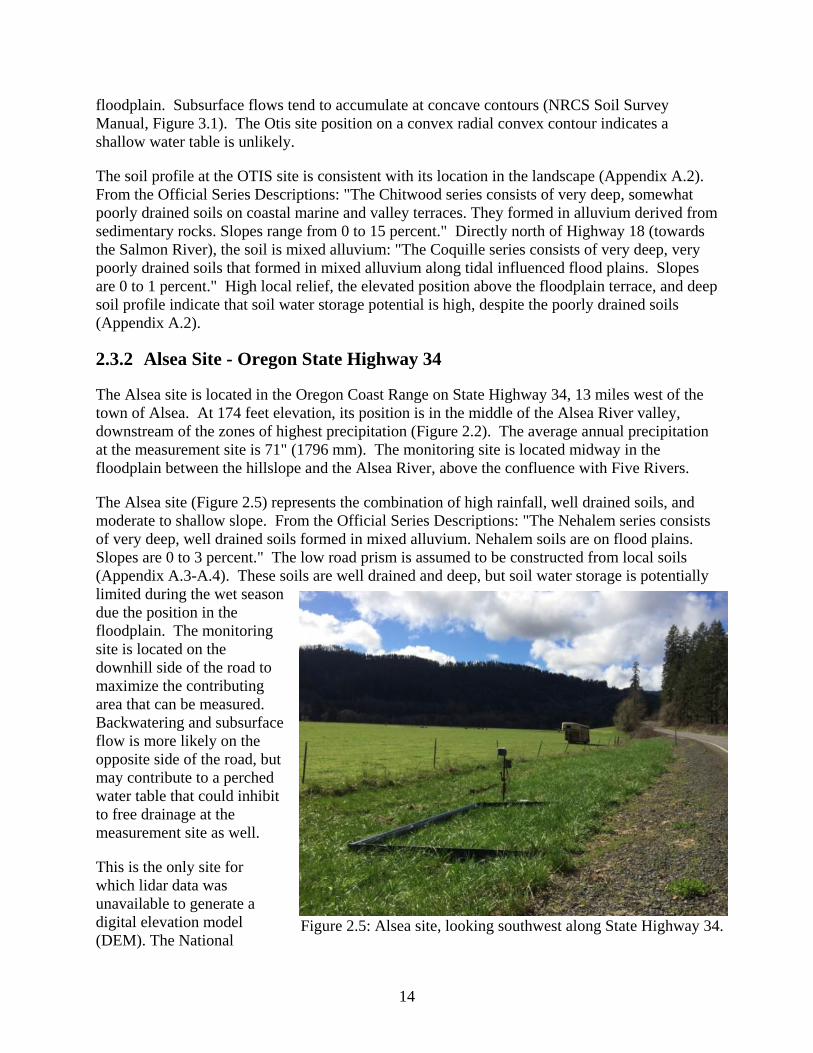
2.3.2 Alsea Site - Oregon State Highway 34

The Alsea site is located in the Oregon Coast Range on State Highway 34, 13 miles west of the town of Alsea. At 174 feet elevation, its position is in the middle of the Alsea River valley, downstream of the zones of highest precipitation (Figure 2.2). The average annual precipitation at the measurement site is 71" (1796 mm). The monitoring site is located midway in the floodplain between the hillslope and the Alsea River, above the confluence with Five Rivers.

The Alsea site (Figure 2.5) represents the combination of high rainfall, well drained soils, and moderate to shallow slope. From the Official Series Descriptions: "The Nehalem series consists of very deep, well drained soils formed in mixed alluvium. Nehalem soils are on flood plains. Slopes are 0 to 3 percent." The low road prism is assumed to be constructed from local soils (Appendix A.3-A.4). These soils are well drained and deep, but soil water storage is potentially limited during the wet season due the position in the floodplain. The monitoring site is located on the downhill side of the road to maximize the contributing area that can be measured. Backwatering and subsurface flow is more likely on the opposite side of the road, but may contribute to a perched water table that could inhibit to free drainage at the measurement site as well.

This is the only site for which lidar data was unavailable to generate a digital elevation model (DEM). The National

Figure 2.5: Alsea site, looking southwest along State Highway 34.

15

Elevation Dataset 10 meter DEM (USGS) was used instead, and consequently the topographic analyses are much coarser in resolution. See Design Guidelines for suggested field methods to augment site analysis for sites where lidar data is not available.

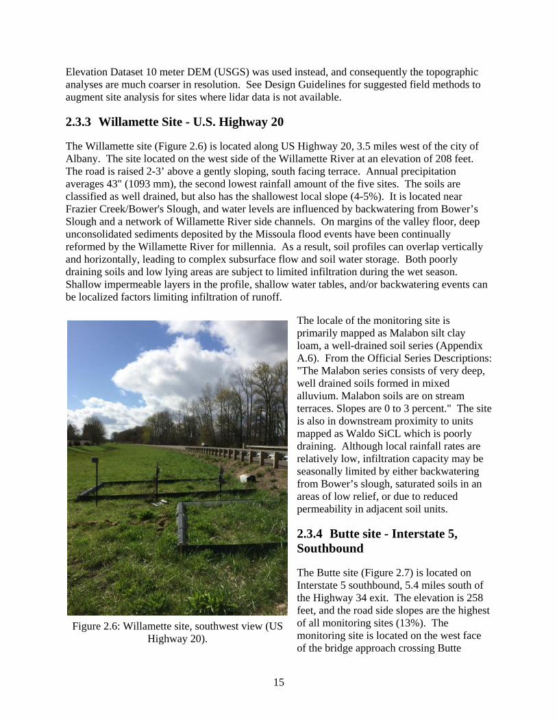
2.3.3 Willamette Site - U.S. Highway 20

The Willamette site (Figure 2.6) is located along US Highway 20, 3.5 miles west of the city of Albany. The site located on the west side of the Willamette River at an elevation of 208 feet. The road is raised 2-3’ above a gently sloping, south facing terrace. Annual precipitation averages 43" (1093 mm), the second lowest rainfall amount of the five sites. The soils are classified as well drained, but also has the shallowest local slope (4-5%). It is located near Frazier Creek/Bower's Slough, and water levels are influenced by backwatering from Bower’s Slough and a network of Willamette River side channels. On margins of the valley floor, deep unconsolidated sediments deposited by the Missoula flood events have been continually reformed by the Willamette River for millennia. As a result, soil profiles can overlap vertically and horizontally, leading to complex subsurface flow and soil water storage. Both poorly draining soils and low lying areas are subject to limited infiltration during the wet season. Shallow impermeable layers in the profile, shallow water tables, and/or backwatering events can be localized factors limiting infiltration of runoff.

The locale of the monitoring site is primarily mapped as Malabon silt clay loam, a well-drained soil series (Appendix A.6). From the Official Series Descriptions: "The Malabon series consists of very deep, well drained soils formed in mixed alluvium. Malabon soils are on stream terraces. Slopes are 0 to 3 percent." The site is also in downstream proximity to units mapped as Waldo SiCL which is poorly draining. Although local rainfall rates are relatively low, infiltration capacity may be seasonally limited by either backwatering from Bower’s slough, saturated soils in an areas of low relief, or due to reduced permeability in adjacent soil units.

2.3.4 Butte site - Interstate 5, Southbound

The Butte site (Figure 2.7) is located on Interstate 5 southbound, 5.4 miles south of the Highway 34 exit. The elevation is 258 feet, and the road side slopes are the highest of all monitoring sites (13%). The monitoring site is located on the west face of the bridge approach crossing Butte

Figure 2.6: Willamette site, southwest view (US Highway 20).

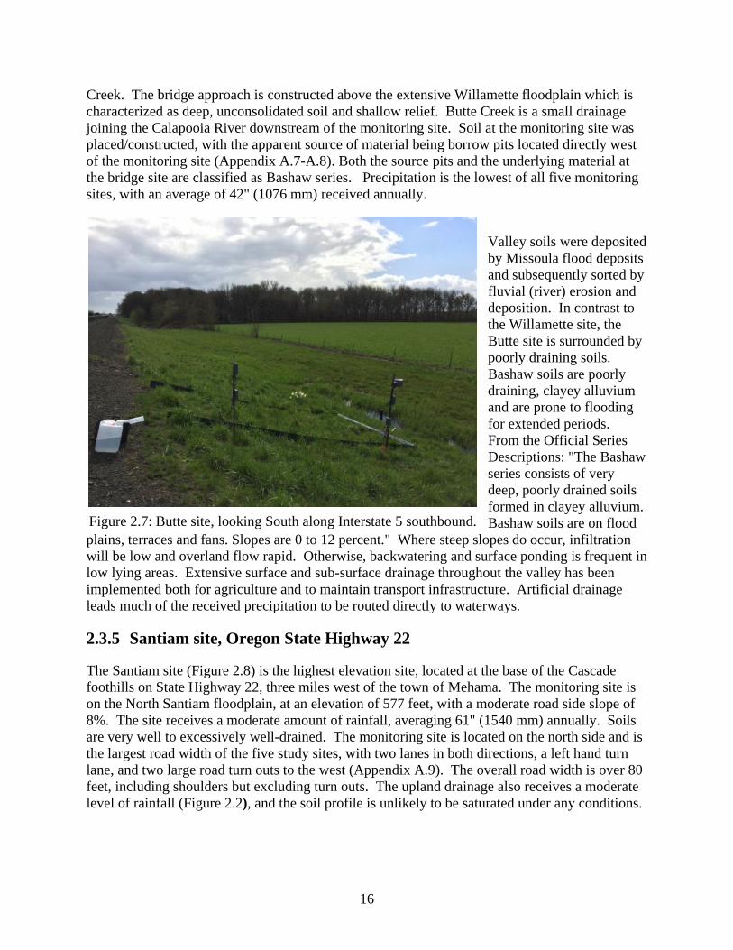
16

Creek. The bridge approach is constructed above the extensive Willamette floodplain which is characterized as deep, unconsolidated soil and shallow relief. Butte Creek is a small drainage joining the Calapooia River downstream of the monitoring site. Soil at the monitoring site was placed/constructed, with the apparent source of material being borrow pits located directly west of the monitoring site (Appendix A.7-A.8). Both the source pits and the underlying material at the bridge site are classified as Bashaw series. Precipitation is the lowest of all five monitoring sites, with an average of 42" (1076 mm) received annually.

Valley soils were deposited by Missoula flood deposits and subsequently sorted by fluvial (river) erosion and deposition. In contrast to the Willamette site, the Butte site is surrounded by poorly draining soils. Bashaw soils are poorly draining, clayey alluvium and are prone to flooding for extended periods. From the Official Series Descriptions: "The Bashaw series consists of very deep, poorly drained soils formed in clayey alluvium. Bashaw soils are on flood

plains, terraces and fans. Slopes are 0 to 12 percent." Where steep slopes do occur, infiltration will be low and overland flow rapid. Otherwise, backwatering and surface ponding is frequent in low lying areas. Extensive surface and sub-surface drainage throughout the valley has been implemented both for agriculture and to maintain transport infrastructure. Artificial drainage leads much of the received precipitation to be routed directly to waterways.

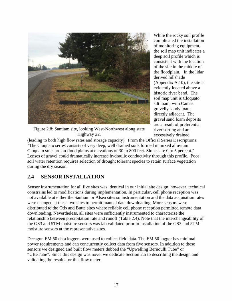
2.3.5 Santiam site, Oregon State Highway 22

The Santiam site (Figure 2.8) is the highest elevation site, located at the base of the Cascade foothills on State Highway 22, three miles west of the town of Mehama. The monitoring site is on the North Santiam floodplain, at an elevation of 577 feet, with a moderate road side slope of 8%. The site receives a moderate amount of rainfall, averaging 61" (1540 mm) annually. Soils are very well to excessively well-drained. The monitoring site is located on the north side and is the largest road width of the five study sites, with two lanes in both directions, a left hand turn lane, and two large road turn outs to the west (Appendix A.9). The overall road width is over 80 feet, including shoulders but excluding turn outs. The upland drainage also receives a moderate level of rainfall (Figure 2.2), and the soil profile is unlikely to be saturated under any conditions.

Figure 2.7: Butte site, looking South along Interstate 5 southbound.

17

While the rocky soil profile complicated the installation of monitoring equipment, the soil map unit indicates a deep soil profile which is consistent with the location of the site in the middle of the floodplain. In the lidar derived hillshade (Appendix A.10), the site is evidently located above a historic river bend. The soil map unit is Cloquato silt loam, with Camas gravelly sandy loam directly adjacent. The gravel sand loam deposits are a result of preferential river sorting and are excessively drained

(leading to both high flow rates and storage capacity). From the Official Series Descriptions: "The Cloquato series consists of very deep, well drained soils formed in mixed alluvium. Cloquato soils are on flood plains at elevations of 30 to 800 feet. Slopes are 0 to 5 percent." Lenses of gravel could dramatically increase hydraulic conductivity through this profile. Poor soil water retention requires selection of drought tolerant species to retain surface vegetation during the dry season.

2.4 SENSOR INSTALLATION

Sensor instrumentation for all five sites was identical in our initial site design, however, technical constrains led to modifications during implementation. In particular, cell phone reception was not available at either the Santiam or Alsea sites so instrumentation and the data acquisition rates were changed at these two sites to permit manual data downloading. More sensors were distributed to the Otis and Butte sites where reliable cell phone reception permitted remote data downloading. Nevertheless, all sites were sufficiently instrumented to characterize the relationship between precipitation rate and runoff (Table 2.4). Note that the interchangeability of the GS3 and 5TM moisture sensors was lab validated prior to installation of the GS3 and 5TM moisture sensors at the representative sites.

Decagon EM 50 data loggers were used to collect field data. The EM 50 logger has minimal power requirements and can concurrently collect data from five sensors. In addition to these sensors we designed and built flow meters dubbed the “Upwelling Bernoulli Tube” or “UBeTube”. Since this design was novel we dedicate Section 2.5 to describing the design and validating the results for this flow meter.

Figure 2.8: Santiam site, looking West-Northwest along state Highway 22.

18

Table 2.4: Instrumentation used in field plots. Variable Sensor Precipitation (ft/day) Decagon ECRN-100 High Resolution Rain Gauge Soil Moisture (-) • Decagon GS3 (additional temperature and electrical conductivity

capability) • Decagon 5TM

Matric Potential (Pa) Decagon MPS-2 dielectric water potential sensor Water Depth (ft) Decagon CTD water level sensor Runoff (ft3/day) UBeTube (Stewart et al. 2015)

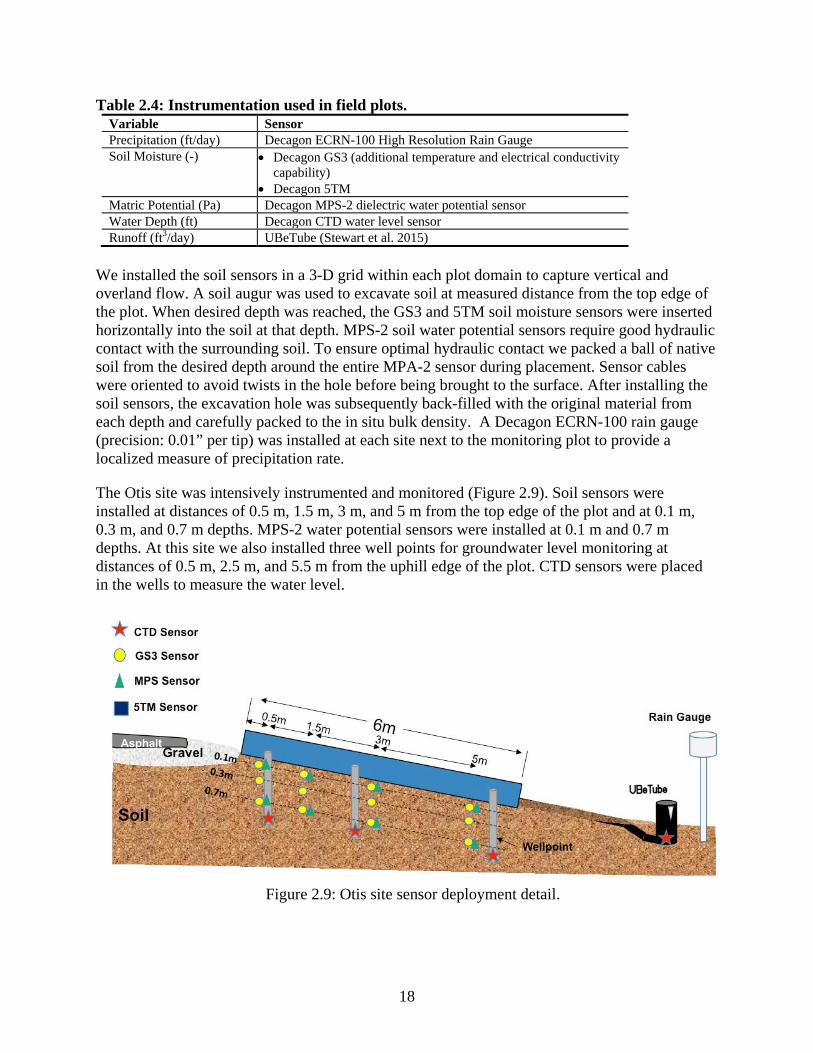
We installed the soil sensors in a 3-D grid within each plot domain to capture vertical and overland flow. A soil augur was used to excavate soil at measured distance from the top edge of the plot. When desired depth was reached, the GS3 and 5TM soil moisture sensors were inserted horizontally into the soil at that depth. MPS-2 soil water potential sensors require good hydraulic contact with the surrounding soil. To ensure optimal hydraulic contact we packed a ball of native soil from the desired depth around the entire MPA-2 sensor during placement. Sensor cables were oriented to avoid twists in the hole before being brought to the surface. After installing the soil sensors, the excavation hole was subsequently back-filled with the original material from each depth and carefully packed to the in situ bulk density. A Decagon ECRN-100 rain gauge (precision: 0.01” per tip) was installed at each site next to the monitoring plot to provide a localized measure of precipitation rate.

The Otis site was intensively instrumented and monitored (Figure 2.9). Soil sensors were installed at distances of 0.5 m, 1.5 m, 3 m, and 5 m from the top edge of the plot and at 0.1 m, 0.3 m, and 0.7 m depths. MPS-2 water potential sensors were installed at 0.1 m and 0.7 m depths. At this site we also installed three well points for groundwater level monitoring at distances of 0.5 m, 2.5 m, and 5.5 m from the uphill edge of the plot. CTD sensors were placed in the wells to measure the water level.

Figure 2.9: Otis site sensor deployment detail.

19

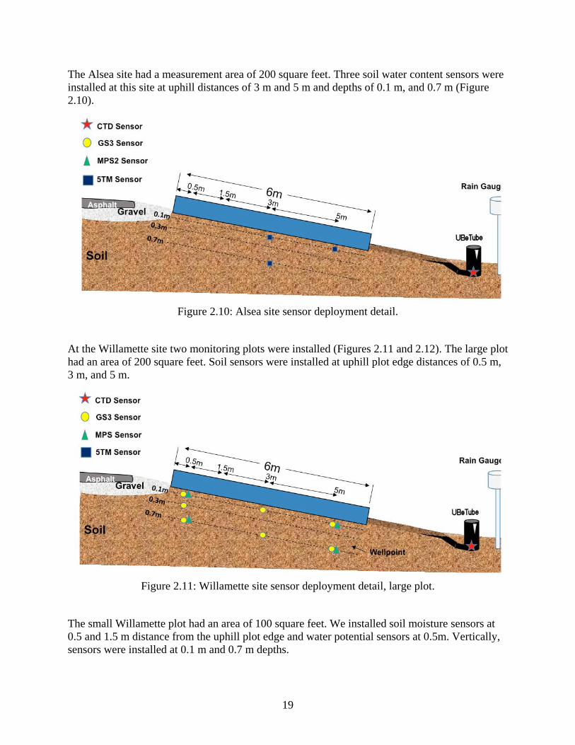
The Alsea site had a measurement area of 200 square feet. Three soil water content sensors were installed at this site at uphill distances of 3 m and 5 m and depths of 0.1 m, and 0.7 m (Figure 2.10).

At the Willamette site two monitoring plots were installed (Figures 2.11 and 2.12). The large plot had an area of 200 square feet. Soil sensors were installed at uphill plot edge distances of 0.5 m, 3 m, and 5 m.

The small Willamette plot had an area of 100 square feet. We installed soil moisture sensors at 0.5 and 1.5 m distance from the uphill plot edge and water potential sensors at 0.5m. Vertically, sensors were installed at 0.1 m and 0.7 m depths.

Figure 2.10: Alsea site sensor deployment detail.

Figure 2.11: Willamette site sensor deployment detail, large plot.

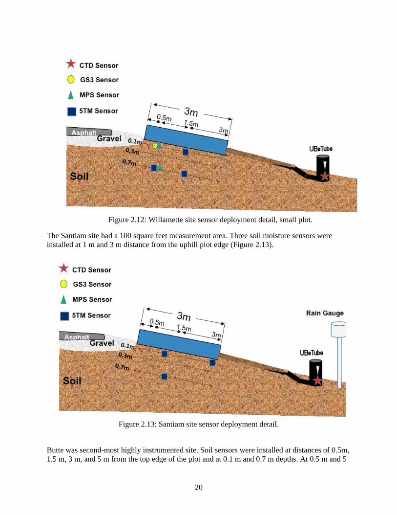
20

The Santiam site had a 100 square feet measurement area. Three soil moisture sensors were installed at 1 m and 3 m distance from the uphill plot edge (Figure 2.13).

Butte was second-most highly instrumented site. Soil sensors were installed at distances of 0.5m, 1.5 m, 3 m, and 5 m from the top edge of the plot and at 0.1 m and 0.7 m depths. At 0.5 m and 5

Figure 2.12: Willamette site sensor deployment detail, small plot.

Figure 2.13: Santiam site sensor deployment detail.

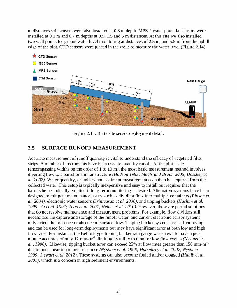
21

m distances soil sensors were also installed at 0.3 m depth. MPS-2 water potential sensors were installed at 0.1 m and 0.7 m depths at 0.5, 1.5 and 5 m distances. At this site we also installed two well points for groundwater level monitoring at distances of 2.5 m, and 5.5 m from the uphill edge of the plot. CTD sensors were placed in the wells to measure the water level (Figure 2.14).

2.5 SURFACE RUNOFF MEASUREMENT

Accurate measurement of runoff quantity is vital to understand the efficacy of vegetated filter strips. A number of instruments have been used to quantify runoff. At the plot-scale (encompassing widths on the order of 1 to 10 m), the most basic measurement method involves diverting flow to a barrel or similar structure (Hudson 1993; Meals and Braun 2006; Dosskey et al. 2007). Water quantity, chemistry and sediment measurements can then be acquired from the collected water. This setup is typically inexpensive and easy to install but requires that the barrels be periodically emptied if long-term monitoring is desired. Alternative systems have been designed to mitigate maintenance issues such as dividing flow into multiple containers (Pinson et al. 2004), electronic water sensors (Srinivasan et al. 2000), and tipping buckets (Hashim et al. 1995; Yu et al. 1997; Zhao et al. 2001; Nehls et al. 2010). However, these are partial solutions that do not resolve maintenance and measurement problems. For example, flow dividers still necessitate the capture and storage of the runoff water, and current electronic sensor systems only detect the presence or absence of surface flow. Tipping bucket systems are self-emptying and can be used for long-term deployments but may have significant error at both low and high flow rates. For instance, the Belfort-type tipping bucket rain gauge was shown to have a per-minute accuracy of only 12 mm-hr-1, limiting its utility to monitor low flow events (Nystuen et al., 1996). Likewise, tipping bucket error can exceed 25% at flow rates greater than 150 mm-hr-1 due to non-linear instrument response (Nystuen et al. 1996; Humphrey et al. 1997; Nystuen 1999; Stewart et al. 2012). These systems can also become fouled and/or clogged (Habib et al. 2001), which is a concern in high sediment environments.

Figure 2.14: Butte site sensor deployment detail.

22

V-notched weirs and flumes have also been used to measure runoff at the plot scale (Hashim et al. 1995; Radatz et al. 2013), as well as for measuring surface runoff in larger catchments (Hudson 1993). However, these installations are often expensive, with a per-plot cost that can exceed US $5,000 (Pinson et al. 2004). Furthermore, maintaining the required up-stream condition of the bed being well below the notch of the weir requires frequent maintenance in natural streams. Stomph et al. (Stomph et al. 2002) designed a flowmeter to measure small discharge rates (2 to 60 L.min-1), in which water enters into and then drains from a chamber filled with small circular orifices. While quite accurate in controlled laboratory conditions, the device is highly sensitive to temperature shifts (due to the use of an air pressure gauge to determine water height), and the orifice configuration needs to be varied depending on the expected range of flows; thus, the device is not well suited for many field conditions.

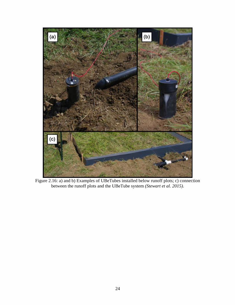
For this study, we needed a low-cost, reliable and accurate method for measuring runoff in the field. We developed a new instrument called the “Upwelling Bernoulli Tube”, or “UBeTube” for short (Stewart et al. 2015). Similar in function to a v-notch weir, the device is self-emptying, features no moving parts, and can be configured to minimize sensitivity to sedimentation. Our tested design possessed the ability to accurately measure flows as low as 0.05 L.min-1 and up to 300 L.min-1 (the latter roughly translating to a runoff rate of 200 mm.hr-1 from a 100 m2 plot), making it ideal for long-term monitoring studies. Best of all, the device can be constructed using commonly-available, low-cost materials, which should enable its widespread use in environmental monitoring studies.

Figure 2.15 illustrates the instrument design. The UBeTube design employed here consisted of a vertical 10 cm (4 inch) diameter pipe with a slot machined into one side. Schedule 40 aluminum pipe (alloy 6063-T52, though others could be used with equal success) was employed due to its relatively low cost, strength, rigidity, resistance to corrosion, and machinability. Schedule 40 or higher PVC may also be used although in our experience the lack of rigidity can make it difficult to accurately machine the slot and thermal stability is of concern with plastics.

Figure 2.15: Schematic and dimensions of the UBeTube design (Stewart et al. 2015).

23

The UBeTube pipe can then be attached to a runoff collection system through use of water-tight neoprene rubber gaskets or similar connection method. The runoff collection system is attached to the bottom of the UBeTube device for several reasons:

• the pressure head needed to drive flow into the pipe is reduced compared to having water enter through the top;

• splashing due to incoming water, which causes pressure fluctuations, is minimized;

• the runoff system piping can be buried below grade, which protects it, buffers temperature swings, and secures the system (Figure 2.16).

It should be noted that having the inflow arrive through the bottom of the pipe could create complicated backwater conditions within the runoff delivery pipe, which can alter the shape and timing of the runoff hydrograph. Thus, in certain situations, it may be preferable to have the inflow enter the UBeTube from the top.

The UBeTube instrument’s machined slot can be any shape and dimension, providing the ability to accurately measure a wide range of discharge rates. Our example system used a slot formed by two superimposed trapezoids: the lower trapezoid had dimensions of 0.2 cm bottom width, 1 cm top width and 10 cm height, while the upper trapezoid had dimensions of 6 cm top width and 6 cm height (Figure 2.15). This allowed the system to be operated with less than 30 cm of pressure head.

24

Figure 2.16: a) and b) Examples of UBeTubes installed below runoff plots; c) connection

between the runoff plots and the UBeTube system (Stewart et al. 2015).

25

2.5.1 Instrument Calibration

By measuring the water height within the pipe, the volumetric flow rate of water through the trapezoidal slot can be calculated using Bernoulli’s equation. Assuming steady-state conditions, the volumetric flow rate (Q) of water through a slot formed from two superimposed trapezoids (such as is shown in Figure 2.15) can be calculated as:

when h0 ≤ h ≤ h1

2

5

1

0123

0 2)(1542

32 hg

hwwchgcwQ −

+= (2.1)

when h1 < h ≤ h2

)))(32)(

52

154(2)(

))((232

)(2)()(

154)(2

32

23

12

5

12

5

1

01

23

12

3

0

25

112

1223

11

hhhhhhgh

wwc

hhhgcw

hhghhwwchhgcwQ

−−−+−

+

−−+

−−−

+−=

(2.2)

when h > h2

)))(32)(

52

154(2)(

))((232)))((

32)(

52

)(154(2

)()())()((2

32

23

12

5

12

5

1

01

23

12

3

02

3

212

5

2

25

112

1223

22

3

11

hhhhhhgh

wwc

hhhgcwhhhhhh

hhghhwwchhhhgcwQ

−−−+−

+

−−+−−−−+

−−−

+−−−=

(2.3)

where h is the water height, g is the gravitational, h0 is the height of the bottom of the slot (bottom of the lower trapezoid), h1 is the height of the lower trapezoid, h2 is the height of the upper trapezoid, w0 is the slot width at the bottom of the lower trapezoid, w1 is the slot width at the transition between trapezoids, w2 is the width at the top of the upper trapezoid, and c is a calibration factor which accounts for non-ideal behaviors. These dimensions are shown in Figure 2.15.

26

Water height was measured with a vented pressure transducer system (Decagon Devices CTD) for its combination of low noise, reliability and economy. For our installations, we placed the water level sensor within a pipe located concentrically inside of the main tube (Figure 2.15). This second pipe had a diameter of 4.2 cm (1 ¼ inch Schedule 40 PVC), and was perforated with 0.6 cm diameter holes beginning 1 cm below the bottom of the height of the slot. This allowed the inner pipe to act as a stilling well with the goal of helping to reduce momentum effects on the water level at high flows and to prevent non-suspended sediment from interfering with the sensor.

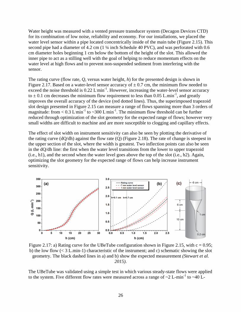
The rating curve (flow rate, Q, versus water height, h) for the presented design is shown in Figure 2.17. Based on a water-level sensor accuracy of ± 0.7 cm, the minimum flow needed to exceed the noise threshold is 0.22 L.min-1. However, increasing the water-level sensor accuracy to ± 0.1 cm decreases the minimum flow requirement to less than 0.05 L.min-1, and greatly improves the overall accuracy of the device (red dotted lines). Thus, the superimposed trapezoid slot design presented in Figure 2.15 can measure a range of flows spanning more than 3 orders of magnitude: from < 0.3 L.min-1 to ~300 L.min-1. The minimum flow threshold can be further reduced through optimization of the slot geometry for the expected range of flows; however very small widths are difficult to machine and are more susceptible to clogging and capillary effects.

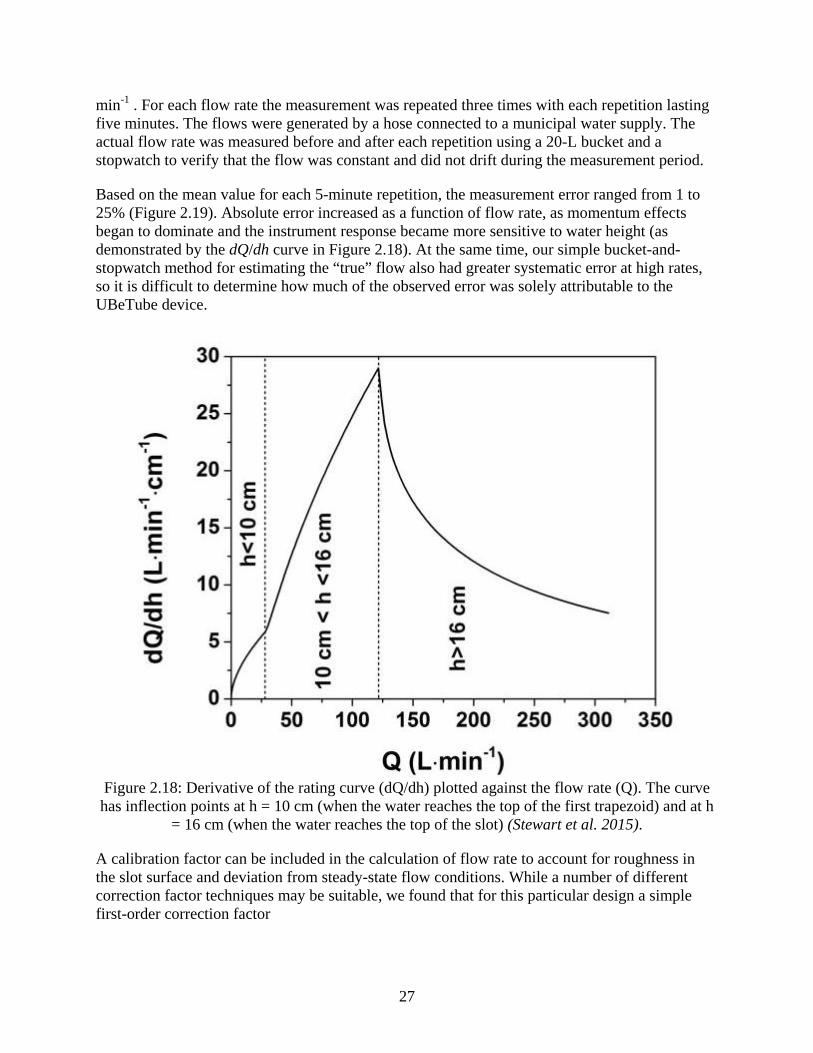
The effect of slot width on instrument sensitivity can also be seen by plotting the derivative of the rating curve (dQ/dh) against the flow rate (Q) (Figure 2.18). The rate of change is steepest in the upper section of the slot, where the width is greatest. Two inflection points can also be seen in the dQ/dh line: the first when the water level transitions from the lower to upper trapezoid (i.e., h1), and the second when the water level goes above the top of the slot (i.e., h2). Again, optimizing the slot geometry for the expected range of flows can help increase instrument sensitivity.

Figure 2.17: a) Rating curve for the UBeTube configuration shown in Figure 2.15, with c = 0.95; b) the low flow (< 3 L.min-1) characteristic of the instrument; and c) schematic showing the slot

geometry. The black dashed lines in a) and b) show the expected measurement (Stewart et al. 2015).

The UBeTube was validated using a simple test in which various steady-state flows were applied to the system. Five different flow rates were measured across a range of ~2 L-min-1 to ~40 L-

27

min-1 . For each flow rate the measurement was repeated three times with each repetition lasting five minutes. The flows were generated by a hose connected to a municipal water supply. The actual flow rate was measured before and after each repetition using a 20-L bucket and a stopwatch to verify that the flow was constant and did not drift during the measurement period.

Based on the mean value for each 5-minute repetition, the measurement error ranged from 1 to 25% (Figure 2.19). Absolute error increased as a function of flow rate, as momentum effects began to dominate and the instrument response became more sensitive to water height (as demonstrated by the dQ/dh curve in Figure 2.18). At the same time, our simple bucket-and-stopwatch method for estimating the “true” flow also had greater systematic error at high rates, so it is difficult to determine how much of the observed error was solely attributable to the UBeTube device.

Figure 2.18: Derivative of the rating curve (dQ/dh) plotted against the flow rate (Q). The curve has inflection points at h = 10 cm (when the water reaches the top of the first trapezoid) and at h

= 16 cm (when the water reaches the top of the slot) (Stewart et al. 2015).

A calibration factor can be included in the calculation of flow rate to account for roughness in the slot surface and deviation from steady-state flow conditions. While a number of different correction factor techniques may be suitable, we found that for this particular design a simple first-order correction factor

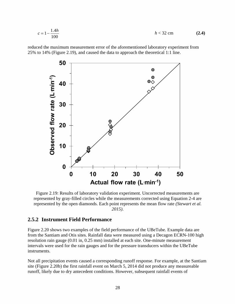
28

1004.11 hc −= h < 32 cm (2.4)

reduced the maximum measurement error of the aforementioned laboratory experiment from 25% to 14% (Figure 2.19), and caused the data to approach the theoretical 1:1 line.

Figure 2.19: Results of laboratory validation experiment. Uncorrected measurements are

represented by gray-filled circles while the measurements corrected using Equation 2-4 are represented by the open diamonds. Each point represents the mean flow rate (Stewart et al.

2015).

2.5.2 Instrument Field Performance

Figure 2.20 shows two examples of the field performance of the UBeTube. Example data are from the Santiam and Otis sites. Rainfall data were measured using a Decagon ECRN-100 high resolution rain gauge (0.01 in, 0.25 mm) installed at each site. One-minute measurement intervals were used for the rain gauges and for the pressure transducers within the UBeTube instruments.

Not all precipitation events caused a corresponding runoff response. For example, at the Santiam site (Figure 2.20b) the first rainfall event on March 5, 2014 did not produce any measureable runoff, likely due to dry antecedent conditions. However, subsequent rainfall events of

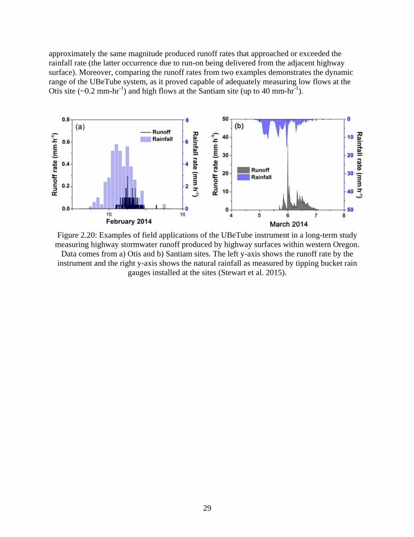
29

approximately the same magnitude produced runoff rates that approached or exceeded the rainfall rate (the latter occurrence due to run-on being delivered from the adjacent highway surface). Moreover, comparing the runoff rates from two examples demonstrates the dynamic range of the UBeTube system, as it proved capable of adequately measuring low flows at the Otis site (~0.2 mm-hr-1) and high flows at the Santiam site (up to 40 mm-hr-1).

Figure 2.20: Examples of field applications of the UBeTube instrument in a long-term study

measuring highway stormwater runoff produced by highway surfaces within western Oregon. Data comes from a) Otis and b) Santiam sites. The left y-axis shows the runoff rate by the

instrument and the right y-axis shows the natural rainfall as measured by tipping bucket rain gauges installed at the sites (Stewart et al. 2015).

30

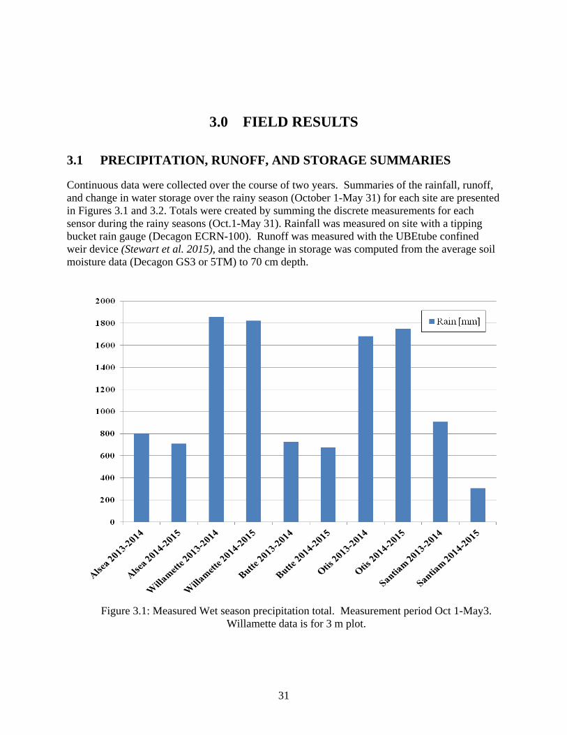
31

3.0 FIELD RESULTS

3.1 PRECIPITATION, RUNOFF, AND STORAGE SUMMARIES

Continuous data were collected over the course of two years. Summaries of the rainfall, runoff, and change in water storage over the rainy season (October 1-May 31) for each site are presented in Figures 3.1 and 3.2. Totals were created by summing the discrete measurements for each sensor during the rainy seasons (Oct.1-May 31). Rainfall was measured on site with a tipping bucket rain gauge (Decagon ECRN-100). Runoff was measured with the UBEtube confined weir device (Stewart et al. 2015), and the change in storage was computed from the average soil moisture data (Decagon GS3 or 5TM) to 70 cm depth.

Figure 3.1: Measured Wet season precipitation total. Measurement period Oct 1-May3.

Willamette data is for 3 m plot.

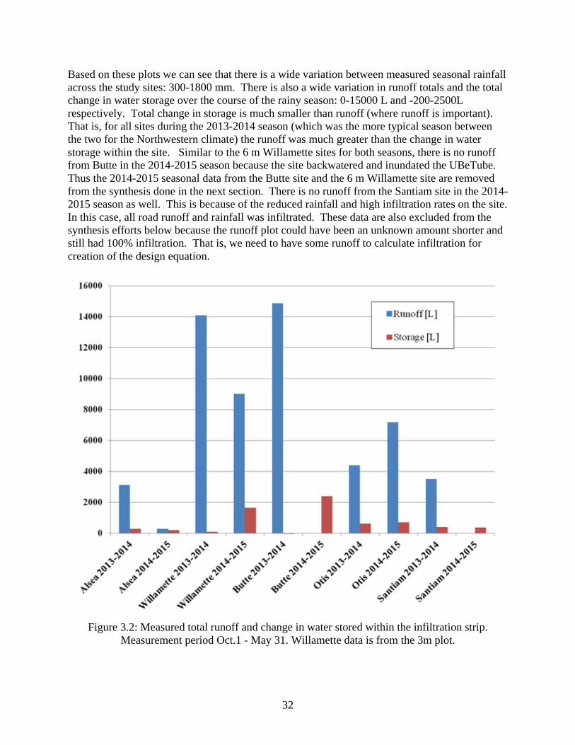
32

Based on these plots we can see that there is a wide variation between measured seasonal rainfall across the study sites: 300-1800 mm. There is also a wide variation in runoff totals and the total change in water storage over the course of the rainy season: 0-15000 L and -200-2500L respectively. Total change in storage is much smaller than runoff (where runoff is important). That is, for all sites during the 2013-2014 season (which was the more typical season between the two for the Northwestern climate) the runoff was much greater than the change in water storage within the site. Similar to the 6 m Willamette sites for both seasons, there is no runoff from Butte in the 2014-2015 season because the site backwatered and inundated the UBeTube. Thus the 2014-2015 seasonal data from the Butte site and the 6 m Willamette site are removed from the synthesis done in the next section. There is no runoff from the Santiam site in the 2014-2015 season as well. This is because of the reduced rainfall and high infiltration rates on the site. In this case, all road runoff and rainfall was infiltrated. These data are also excluded from the synthesis efforts below because the runoff plot could have been an unknown amount shorter and still had 100% infiltration. That is, we need to have some runoff to calculate infiltration for creation of the design equation.

Figure 3.2: Measured total runoff and change in water stored within the infiltration strip.

Measurement period Oct.1 - May 31. Willamette data is from the 3m plot.

33

Time series of the rainfall and runoff along with time series of soil moisture measurements for each site are presented in Figures 3.3-3.7 in Section 3.3 Time Series Plots of Monitoring Data.

3.2 DATA FROM MONITORING SITES

Alsea had a moderate slope and rainfall, yet this site saw some of the most dramatic runoff events (out of the observation plots). In particular, the peak runoffs seen near January of 2014 and 2015 are associated with the upper soil layer coming to saturation. This indicates that the loading rates (or rainfall and road runoff) exceeded the potential infiltration rated for these events. Overland flow due to the first flush event of 2013 is also visible in this plot; however, no overland flow occurred in the first rainfall events of 2014. In total this first flush event did not contribute significantly to the total volume of water that was infiltrated over the course of the observational campaign.

Santiam was the site with the highest soil conductivities and some of the lowest rainfall. The end result is clear; this was one of the most effective places for infiltration. One hundred percent of the total water loading due to road runoff and precipitation was infiltrated in the 2014-2015 season (recall that 2014-2015 was particularly dry). Minimal runoff from the infiltration plot was measured throughout the entire 2 year period. A first flush event is visible in 2013; however, it again is small compared to the total water infiltrated into the strip.

Willamette had high rainfall totals, a gentle slope, and a moderately well-drained soil. Again, most of the water loading onto the observation plot was infiltrated. In this site, plot runoff is associated with the rise of the water table from below, seen as the saturation of the lower soil layers in the soil moisture plot. This region was also prone to ponding in low-lying areas and had the potential to create backwatering restriction on the overall flow of water through the subsurface. Negligible first flush events are seen at this site as well.

Butte had the highest overland flow percentages of all the sites. It was steep and had the least permeable soils—a heavy clay Bashaw. In addition, the water table rose significantly through the rainy season, decreasing the capacity of the infiltration strip. Runoff is correlated with rainfall events and groundtable rise. This site was also prone to backwatering. During the 2014-2015 wet season the area flooded. This flooding contaminated the signal from the UBeTube, and the runoff data was discarded. First flush events are visible but not as large as the runoff events in the middle of the rainy season.

Otis is located near the coast and had the highest expected rainfall. The actual rainfall measured was similar to the Willamette site. Little runoff occurred in both rainy seasons of observation. Total porosity at this site is greater than the others, as the soil had a sandy character. First flush overland flow did not occur.

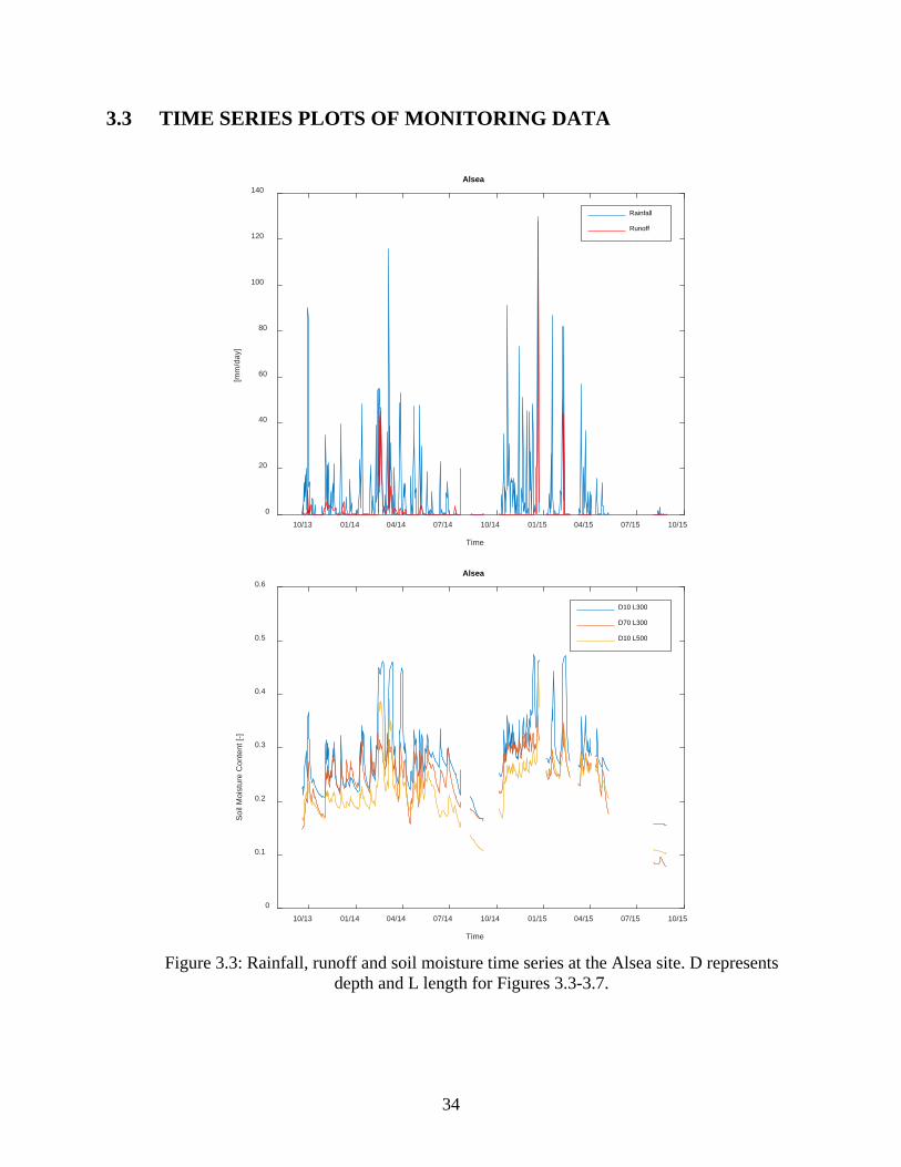
34

3.3 TIME SERIES PLOTS OF MONITORING DATA

Figure 3.3: Rainfall, runoff and soil moisture time series at the Alsea site. D represents

depth and L length for Figures 3.3-3.7.

10/13 01/14 04/14 07/14 10/14 01/15 04/15 07/15 10/15

Time

0

20

40

60

80

100

120

140

[mm

/day

]

Alsea

Rainfall

Runoff

10/13 01/14 04/14 07/14 10/14 01/15 04/15 07/15 10/15

Time

0

0.1

0.2

0.3

0.4

0.5

0.6

Soi

l Moi

stur

e C

onte

nt [-

]

Alsea

D10 L300

D70 L300

D10 L500

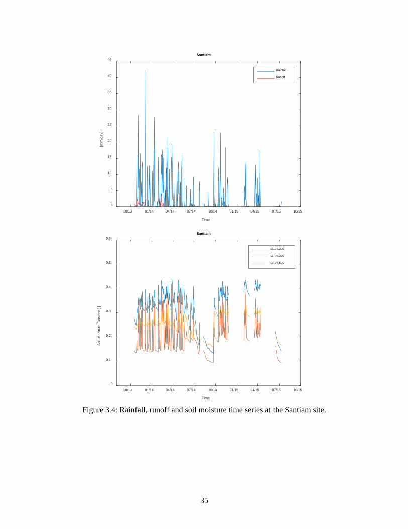
35

Figure 3.4: Rainfall, runoff and soil moisture time series at the Santiam site.

10/13 01/14 04/14 07/14 10/14 01/15 04/15 07/15 10/15

Time

0

5

10

15

20

25

30

35

40

45

[mm

/day

]

Santiam

Rainfall

Runoff

10/13 01/14 04/14 07/14 10/14 01/15 04/15 07/15 10/15

Time

0

0.1

0.2

0.3

0.4

0.5

0.6

Soi

l Moi

stur

e C

onte

nt [-

]

Santiam

D10 L300

D70 L300

D10 L500

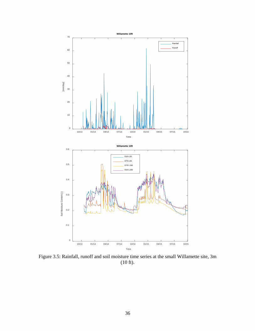
36

Figure 3.5: Rainfall, runoff and soil moisture time series at the small Willamette site, 3m

(10 ft).

10/13 01/14 04/14 07/14 10/14 01/15 04/15 07/15 10/15

Time

0

10

20

30

40

50

60

70

[mm

/day

]

Willamette 10ft

Rainfall

Runoff

10/13 01/14 04/14 07/14 10/14 01/15 04/15 07/15 10/15

Time

0

0.1

0.2

0.3

0.4

0.5

0.6

Soi

l Moi

stur

e C

onte

nt [-

]

Willamette 10ft

D10 L50

D70 L50

D70 L150

D10 L150

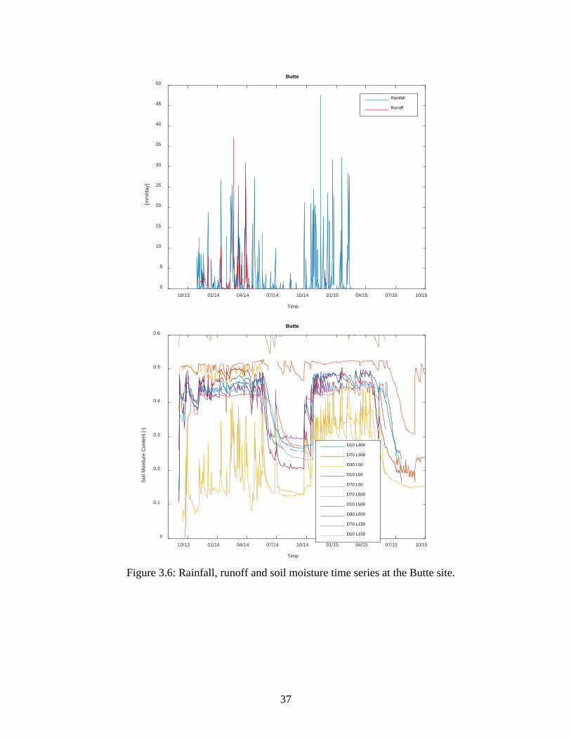
37

Figure 3.6: Rainfall, runoff and soil moisture time series at the Butte site.

10/13 01/14 04/14 07/14 10/14 01/15 04/15 07/15 10/15

Time

0

5

10

15

20

25

30

35

40

45

50

[mm

/day

]

Butte

Rainfall

Runoff

10/13 01/14 04/14 07/14 10/14 01/15 04/15 07/15 10/15

Time

0

0.1

0.2

0.3

0.4

0.5

0.6

Soi

l Moi

stur

e C

onte

nt [-

]

Butte

D10 L300

D70 L300

D30 L50

D10 L50

D70 L50

D70 L500

D10 L500

D30 L500

D70 L150

D10 L150

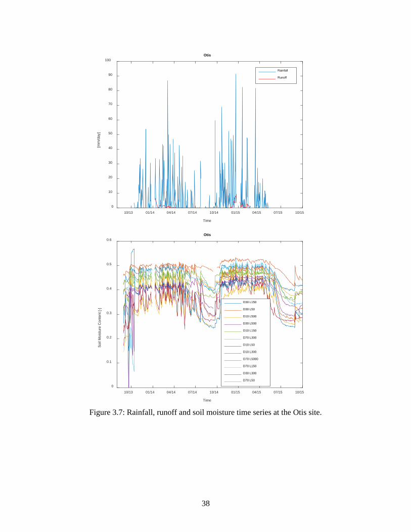
38

Figure 3.7: Rainfall, runoff and soil moisture time series at the Otis site.

10/13 01/14 04/14 07/14 10/14 01/15 04/15 07/15 10/15

Time

0

10

20

30

40

50

60

70

80

90

100

[mm

/day

]

Otis

Rainfall

Runoff

10/13 01/14 04/14 07/14 10/14 01/15 04/15 07/15 10/15

Time

0

0.1

0.2

0.3

0.4

0.5

0.6

Soi

l Moi

stur

e C

onte

nt [-

]

Otis

D30 L150

D30 L50

D10 L500

D30 L500

D10 L150

D70 L300

D10 L50

D10 L300

D70 L5000

D70 L150

D30 L300

D70 L50

39

3.4 MONITORING DATA SUMMARY

In general these results show that the 2014-2015 wet season was shorter in duration, although the total rainfall amounts are similar for most sites. The major exception is the Santiam site which experienced significantly less precipitation in the 2014-2015 rainy season. The time series also indicate that at the individual storm level, runoff can occur in several ways: 1) the surface can become saturated, creating a barrier to infiltration. This behavior is responsible for the largest runoff events at the Alsea site. 2) The water table can rise (D70 L50 soil moisture read-out rises sharply then plateaus), reducing the capacity of the infiltration strip. This behavior is responsible for the largest runoff events at the Butte site. This behavior is also associated with backwatering and surface ponding in the low-lying areas below the filter strip (also observed at the Butte site). 3) Intense precipitation overwhelms infiltration rates. One example is found in the peak runoff event 2014-2015 rainy season at the Alsea site. First flush events, defined as the runoff events that occur coincident with the first major rainfall event at the beginning of the wet season events are sometimes hypothesized to carry large amounts of dust debris and pollutants. In the measured dataset, these events are not responsible for a significant fraction of the runoff over the season. First flush runoff events were infiltrated completely at the Otis and Willamette sites and represented small contributions to the overall runoff totals at Butte, Santiam and Alsea. Figure 3.8 summarizes data from all sites.

A traditional approach for VFS design would specify a design storm event, then determine the necessary width to infiltrate the water from the designated storm. A critical view of the infiltration traces above reveals that this approach may not be fruitful as the actual infiltration (runoff) also depends on the timing of the event. Antecedent conditions play a larger role in the infiltration capacity at any given moment than we expected. That is, some of the larger recorded storms did not produce runoff within our record, and storms with similar intensities within the same season produced vastly different runoff behaviors depending on their soil moisture content. So, while the ‘designated storm event’ approach is viable in regions where there is a significant time between storms for the system to reset, in western Oregon, a more fruitful approach may be to specify a ‘design seasonal rainfall’. We proceed from the assumption that the total infiltrated water over the entire season is the variable that the design wishes to control. Thus the analysis is focused on seasonal rainfall and runoff totals.

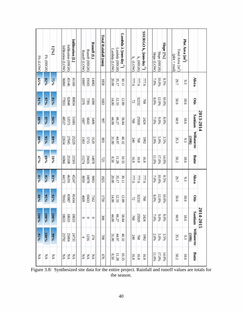
40

Figure 3.8: Synthesized site data for the entire project. Rainfall and runoff values are totals for

the season.

Alsea

Otis

SantiamW

illamette

(10ft)B

utteA

lseaO

tisSantiam

Willam

ette(10ft)

Butte

Plot Area [m

2]9.3

18.618.6

9.318.6

9.318.6

18.69.3

18.6

Total Area [m

2] (plot + road)

29.750.6

60.935.3

50.229.7

50.660.9

35.350.2

Slope [%]

8.5%10.0%

8.0%3.5%

14.0%8.5%

10.0%8.0%

3.5%14.0%

Slope (HIG

H)

10.0%12.0%

9.0%5.0%

17.0%10.0%

12.0%9.0%

5.0%17.0%

Slope (LOW

)7.0%

8.0%7.0%

2.0%11.0%

7.0%8.0%

7.0%2.0%

11.0%

SSUR

GO

ks [m

m⋅day

-1]777.6

7682424

199216.8

777.6768

24241992

16.8k

s (HIG

H)

777.632232

25920768

16.8777.6

3223225920

76816.8

ks (LO

W)

777.672

768240

16.8777.6

72768

24016.8

Lambda λ [m

m⋅day

-1]30.11

12.8958.84

40.3210.35

30.1112.89

58.8440.32

10.35Lam

bda (HIG

H)

35.1712.33

66.2744.97

11.2835.17

12.3366.27

44.9711.28

Lambda (LO

W)

20.0014.00

44.0031.00

8.5020.00

14.0044.00

31.008.50

Total Rainfall (m

m)

18581683

907803

7251825

1750306

708676

Runoff (L)

140824390

34993120

148789003

71620

274N

AR

unoff (HIG

H)

191837391

66435715

1941610078

104330

1216N

AR

unoff (LOW

)10097

23761607

130311274

80594609

04

NA

Infiltration [L]41160

8083451681

2522921503

4524781434

1863324735

NA

Infiltration (HIG

H)

4514682848

5357327045

2510846191

8398718633

25004N

AInfiltration (LO

W)

3606077833

4853722634

1696644172

7816318633

23792N

A

I [%]

75%95%

94%89%

59%83%

92%100%

99%N

A

I% (H

IGH

)82%

97%97%

95%69%

85%95%

100%100%

NA

I% (LO

W)

65%91%

88%80%

47%81%

88%100%

95%N

A

2013-20142014-2015

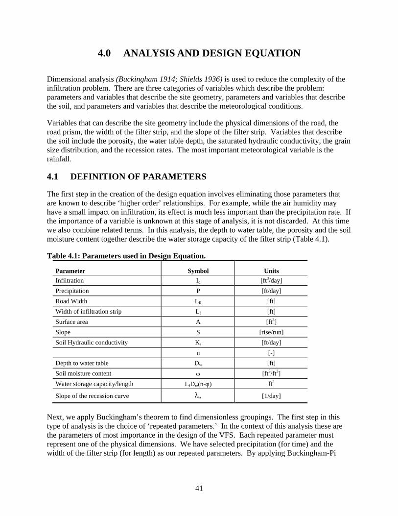
41

4.0 ANALYSIS AND DESIGN EQUATION

Dimensional analysis (Buckingham 1914; Shields 1936) is used to reduce the complexity of the infiltration problem. There are three categories of variables which describe the problem: parameters and variables that describe the site geometry, parameters and variables that describe the soil, and parameters and variables that describe the meteorological conditions.

Variables that can describe the site geometry include the physical dimensions of the road, the road prism, the width of the filter strip, and the slope of the filter strip. Variables that describe the soil include the porosity, the water table depth, the saturated hydraulic conductivity, the grain size distribution, and the recession rates. The most important meteorological variable is the rainfall.

4.1 DEFINITION OF PARAMETERS

The first step in the creation of the design equation involves eliminating those parameters that are known to describe ‘higher order’ relationships. For example, while the air humidity may have a small impact on infiltration, its effect is much less important than the precipitation rate. If the importance of a variable is unknown at this stage of analysis, it is not discarded. At this time we also combine related terms. In this analysis, the depth to water table, the porosity and the soil moisture content together describe the water storage capacity of the filter strip (Table 4.1).

Table 4.1: Parameters used in Design Equation.

Parameter Symbol Units Infiltration Ic [ft3/day] Precipitation P [ft/day] Road Width LR [ft] Width of infiltration strip Lf [ft] Surface area A [ft3] Slope S [rise/run] Soil Hydraulic conductivity Ks [ft/day]

n [-] Depth to water table Dw [ft] Soil moisture content ϕ [ft3/ft3] Water storage capacity/length LfDw(n-ϕ) ft2

Slope of the recession curve *λ [1/day]

Next, we apply Buckingham’s theorem to find dimensionless groupings. The first step in this type of analysis is the choice of ‘repeated parameters.’ In the context of this analysis these are the parameters of most importance in the design of the VFS. Each repeated parameter must represent one of the physical dimensions. We have selected precipitation (for time) and the width of the filter strip (for length) as our repeated parameters. By applying Buckingham-Pi

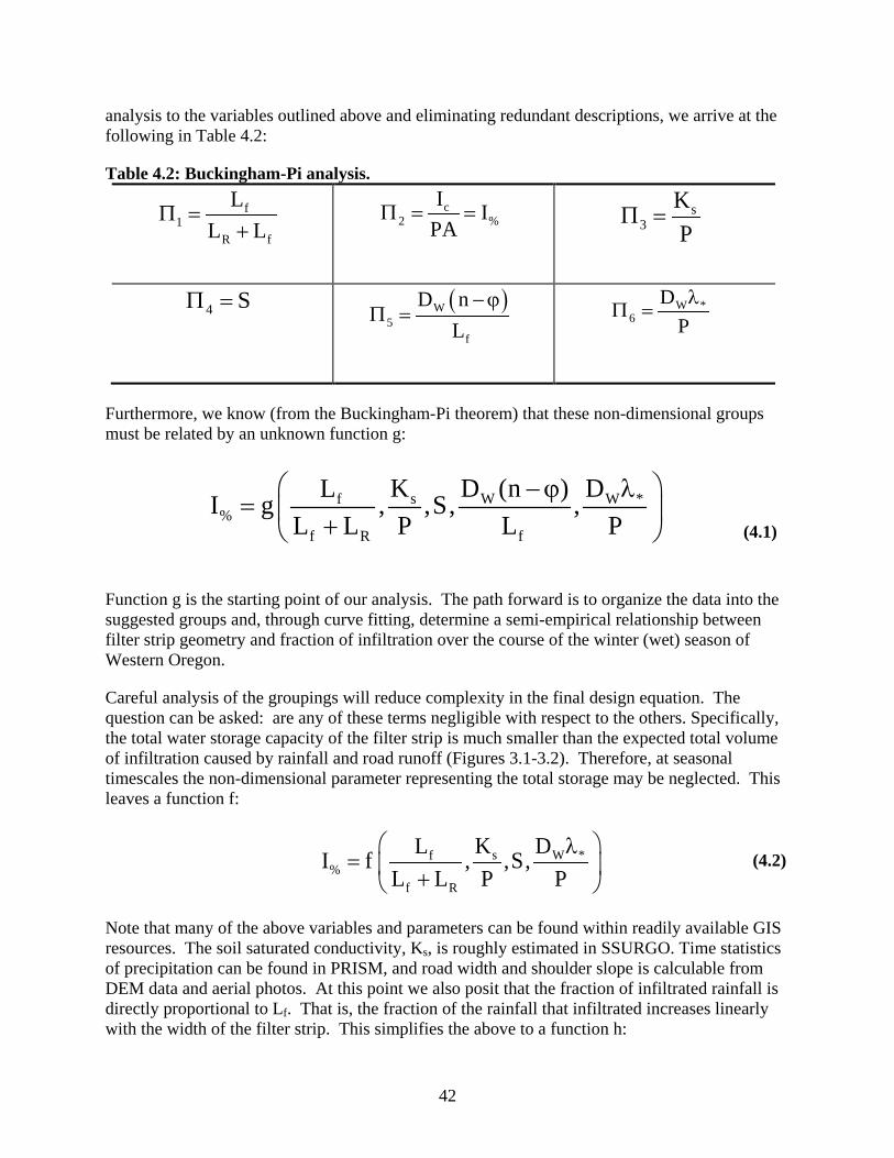
42

analysis to the variables outlined above and eliminating redundant descriptions, we arrive at the following in Table 4.2:

Table 4.2: Buckingham-Pi analysis.

f1

R f

LL L

Π =+

c2 %

I IPA

=Π = s3

KP

Π =

4 SΠ = ( )W5

f

D nL

Π−ϕ

= W *

6D

PΠ

λ=

Furthermore, we know (from the Buckingham-Pi theorem) that these non-dimensional groups must be related by an unknown function g:

Function g is the starting point of our analysis. The path forward is to organize the data into the suggested groups and, through curve fitting, determine a semi-empirical relationship between filter strip geometry and fraction of infiltration over the course of the winter (wet) season of Western Oregon.

Careful analysis of the groupings will reduce complexity in the final design equation. The question can be asked: are any of these terms negligible with respect to the others. Specifically, the total water storage capacity of the filter strip is much smaller than the expected total volume of infiltration caused by rainfall and road runoff (Figures 3.1-3.2). Therefore, at seasonal timescales the non-dimensional parameter representing the total storage may be neglected. This leaves a function f:

s W *f%

f R

K DLI f , ,S,L L P P

= +

λ

Note that many of the above variables and parameters can be found within readily available GIS resources. The soil saturated conductivity, Ks, is roughly estimated in SSURGO. Time statistics of precipitation can be found in PRISM, and road width and shoulder slope is calculable from DEM data and aerial photos. At this point we also posit that the fraction of infiltrated rainfall is directly proportional to Lf. That is, the fraction of the rainfall that infiltrated increases linearly with the width of the filter strip. This simplifies the above to a function h:

s W Wf%

f R f

*K D (n ) DLI g , ,S, ,L L P L P

−ϕ= +

λ

(4.1)

(4.2)

43

%f

*s Wf R K DL LI h ,S,L P P

+ =

λ

The most problematic parameter within this analysis is Ks since it tends to be highly variable in space, and is the most difficult to measure. In SSURGO, there are typically ranges of Ks that vary over 1-4 orders of magnitude. Recall that there are three types of variables that will describe the infiltration: soil, weather, and site geometry. The first and third independent parameter in the right hand side of the above equation both endeavor to describe the same physical process, the rate of subsurface water movement. If there is a correlation between *WD λ and Ks, then both variables would not be needed. Moving forward, we define

Where ∆t is 1 day, and D is the depth of the soil moisture profile (700 mm for all of the sites), measured in mm, and ϕm is the depth averaged soil moisture content, at each sampling time. We are substituting depth to water table with depth of measurement here since water table was not measured at all sites. Within this framework, our pseudo-equation becomes:

mDt

∆ϕλ = −

∆

sf R%

f

L LI h ,S,L P P

K + =

λ

(4.3)

(4.4)

(4.5)

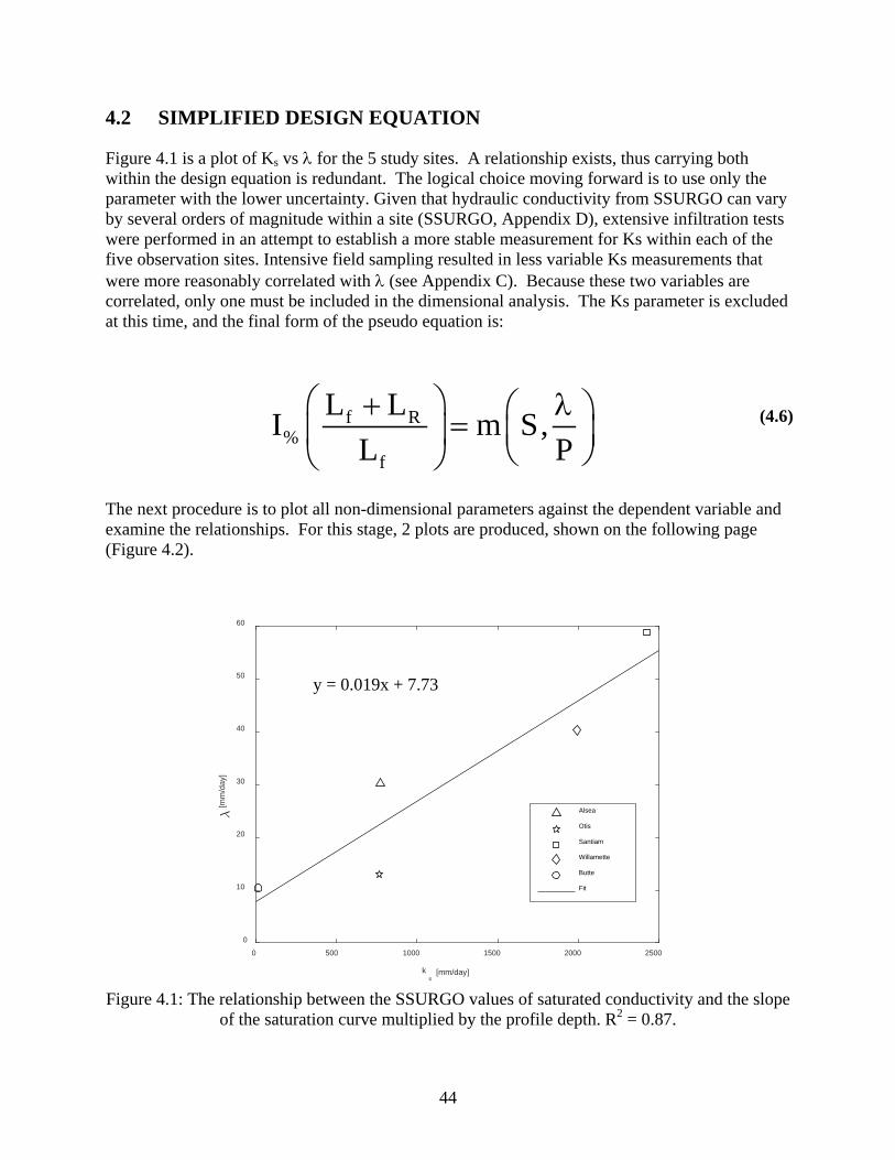
44

4.2 SIMPLIFIED DESIGN EQUATION

Figure 4.1 is a plot of Ks vs λ for the 5 study sites. A relationship exists, thus carrying both within the design equation is redundant. The logical choice moving forward is to use only the parameter with the lower uncertainty. Given that hydraulic conductivity from SSURGO can vary by several orders of magnitude within a site (SSURGO, Appendix D), extensive infiltration tests were performed in an attempt to establish a more stable measurement for Ks within each of the five observation sites. Intensive field sampling resulted in less variable Ks measurements that were more reasonably correlated with λ (see Appendix C). Because these two variables are correlated, only one must be included in the dimensional analysis. The Ks parameter is excluded at this time, and the final form of the pseudo equation is:

The next procedure is to plot all non-dimensional parameters against the dependent variable and examine the relationships. For this stage, 2 plots are produced, shown on the following page (Figure 4.2).

Figure 4.1: The relationship between the SSURGO values of saturated conductivity and the slope

of the saturation curve multiplied by the profile depth. R2 = 0.87.

0 500 1000 1500 2000 2500

ks

[mm/day]

0

10

20

30

40

50

60

[mm

/day

]

Alsea

Otis

Santiam

Willamette

Butte

Fit

f R%

f

L LI m S,L P

+ =

λ (4.6)

y = 0.019x + 7.73

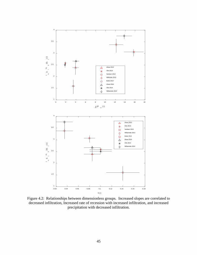
45

Figure 4.2: Relationships between dimensionless groups. Increased slopes are correlated to decreased infiltration, Increased rate of recession with increased infiltration, and increased

precipitation with decreased infiltration.

0 2 4 6 8 10 12 14 16 18

/(Pm

) [-]

1

1.5

2

2.5

3

3.5

4

I %(L

f+LR

)/(L

f) [-]

Alsea 2013

Otis 2013

Santiam 2013

Willmette 2013

Butte 2013

Alsea 2014

Otis 2014

Willamette 2014

0.02 0.04 0.06 0.08 0.1 0.12 0.14 0.16 0.18

S [-]

1

1.5

2

2.5

3

3.5

4

I %(L

f+LR

)/(L

f) [-]

Alsea 2013

Otis 2013

Santiam 2013

Willamette 2013

Butte 2013

Alsea 2014

Otis 2014

Willamette 2014

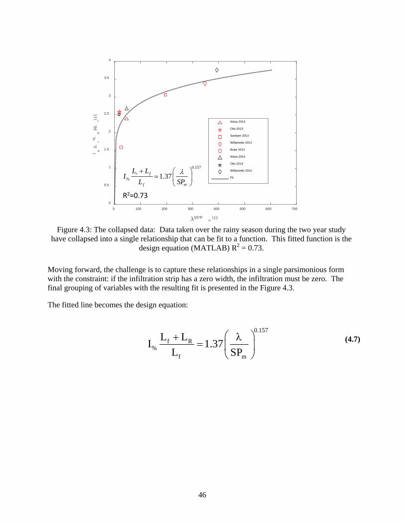
46

Moving forward, the challenge is to capture these relationships in a single parsimonious form with the constraint: if the infiltration strip has a zero width, the infiltration must be zero. The final grouping of variables with the resulting fit is presented in the Figure 4.3.

The fitted line becomes the design equation:

0.157

f R%

f m

L LI 1.37L SP

λ +=

Figure 4.3: The collapsed data: Data taken over the rainy season during the two year study

have collapsed into a single relationship that can be fit to a function. This fitted function is the design equation (MATLAB) R2 = 0.73.

0 100 200 300 400 500 600 700

/(S*Pm

) [-]

0

0.5

1

1.5

2

2.5

3

3.5

4

I %(L

f+LR

)/(L

f) [-]

Alsea 2013

Otis 2013

Santiam 2013

Willamette 2013

Butte 2013

Alsea 2014

Otis 2014

Willamette 2014

Fit

0.157

% 1.37r f

f m

L LI

L SPλ+

=

R2=0.73

(4.7)

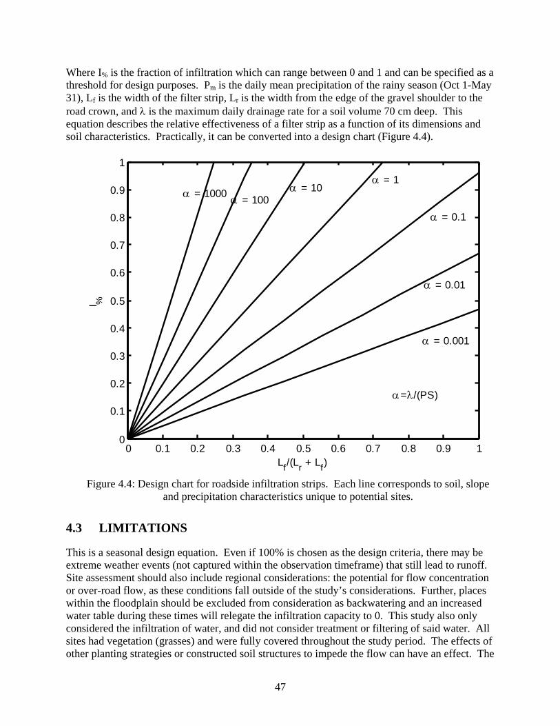
47

Where I% is the fraction of infiltration which can range between 0 and 1 and can be specified as a threshold for design purposes. Pm is the daily mean precipitation of the rainy season (Oct 1-May 31), Lf is the width of the filter strip, Lr is the width from the edge of the gravel shoulder to the road crown, and λ is the maximum daily drainage rate for a soil volume 70 cm deep. This equation describes the relative effectiveness of a filter strip as a function of its dimensions and soil characteristics. Practically, it can be converted into a design chart (Figure 4.4).

4.3 LIMITATIONS

This is a seasonal design equation. Even if 100% is chosen as the design criteria, there may be extreme weather events (not captured within the observation timeframe) that still lead to runoff. Site assessment should also include regional considerations: the potential for flow concentration or over-road flow, as these conditions fall outside of the study’s considerations. Further, places within the floodplain should be excluded from consideration as backwatering and an increased water table during these times will relegate the infiltration capacity to 0. This study also only considered the infiltration of water, and did not consider treatment or filtering of said water. All sites had vegetation (grasses) and were fully covered throughout the study period. The effects of other planting strategies or constructed soil structures to impede the flow can have an effect. The

Figure 4.4: Design chart for roadside infiltration strips. Each line corresponds to soil, slope

and precipitation characteristics unique to potential sites.

0 0.1 0.2 0.3 0.4 0.5 0.6 0.7 0.8 0.9 10

0.1

0.2

0.3

0.4

0.5

0.6

0.7

0.8

0.9

1

I %

Lf/(Lr + Lf)

α = 0.001

α = 0.01

α = 0.1

α = 10α = 100α = 1000

α=λ/(PS)

α = 1

48

design equation will likely provide insight in this case as a minimum infiltration boundary. We hypothesize that the ‘equivalent slope’ could be used in this scenario, but additional studies would be required to verify the design equation in this extension of its intended scope. Equivalent slope is an adjustment to the embanckment slope due to the presence of vegetation. The equivalent slope of an embankement with dense vegetation would be less than the same slope with no vegetation.

4.4 SUMMARY OF DESIGN PROCESS

The design process should be achieved through a series of steps: information gathering, vetting of information, and the design calculation (see also Section 4.6 Design Flow Chart). Information gathering involves analysis of digital elevation maps, the NRCS soil survey and the PRISM climate data:

COLLECT RELEVENT SPATIAL DATA 1) Obtain a DEM of the area of interest (AOI). LiDAR data exists for much of Oregon, and

high resolution digital elevation maps are available. If lidar is not available for the area of interest, the 10 m DEM of the country is available through the National Geospatial Data Gateway. Once the potential VFS site has been identified within the DEM:

a) A quality check on the DEM should be performed: Can the road prism be detected? Is there sufficient resolution to determine slopes of the road shoulder? If not, then an on the ground site survey is required.

b) Calculate hillshade raster and percent slope for AOI.

c) Flow concentration can also be calculated at this time to determine if , due to confluences in the topography, roadcuts, or other features will lead increases in runoff intensity. Under these scenarios, the site should be rejected.

d) Determine if the proposed VFS site is in a floodplain. Sites that reside within the floodplain should also be rejected. Consult FEMA Maps. (www.oregonriskmaps.com)

2) Obtain the SSURGO soils data (web based) and Official Series Description (OSD) and for soils in your AOI from the NRCS Soil Survey (USDA 2003; USDA 2002). Soil survey data are available through the NRCS Web Soil Survey interface (http://websoilsurvey.sc.egov.usda.gov/). The database is also accessible through a Google Earth KML or can be downloaded as a shapefile/geodatabase through the National Data Gateway.

a) Delineate the AOI in the map interface. Export the polygons of soil classification. Soil classification polygons range widely in size. Each soil class that intersects with the potential position of the VFS design should noted.

b) Several soil series may be listed in the Soil Map Unit. Based on site slope and aspect, determine the most likely series. The OSD describes “competing series” as suggested alrternatives which may match your site better than the Soil Survey, especially in those

49

cases where the road was built on transported material. The OSD and SSURGO data for each soil polygon can be downloaded directly from the web interface.

c) The soil depth and the saturated hydraulic conductivity should be extracted from the SSURGO tables. The saturated hydraulic conductivity will be listed as a range. If this range spans more than 2 orders of magnitude, a site visit is needed to measure the slope of the saturation curve. Otherwise, a first approximation of λ (from Figure 4.1) can be made using the relationship s0.019K 7.73λ = + The units for Ks in this equation are mm/day.

d) A range of slopes is also given within the soil description. A check should be performed against the slope calculations performed in (1). If there is a disagreement, a site survey should be performed.

e) Note the soil Hydrologic drainage class.

3) Obtain rainfall data from the PRISM Climate server (http://www.prism.oregonstate.edu/). This model generates maps of the 30 year normal annual and monthly precipitation throughout the continental US, interpolating 30 year climate data to generate maps with 800 m resolution. These maps can downloaded as rasters, or precipitation level can be used directly.

a) Extract the monthly totals for October-May, and compute the average daily wet season precipitation (October-May Precip ÷ 241 days).

b) Evaluate local and basin precipitation in the upstream drainage. Is this an area with extreme rainfall? A site with precipitation in excess of 2m (6.54 ft) per year would classify as high precipation. Is the site prone to flooding during high flow in local waterways? Sites within the flood plain or below the high-water mark of nearby water-ways are likely prone to flooding.

4) Site visit for data collection: if a site visit was triggered in (1) or (2) above, then additional measurements are needed to complete a first design calculation.

a) A site survey would take the necessary data to determine the slope of the vegetated area immediately adjacent to the gravel shoulder. In addition this survey should collect data about the broader hydrological context of the proposed site: extent of any nearest low-lying areas where ponding or backwatering may occur, proximity to stream channels, the position of the road crown, the potential for flow concentration.

b) Measure the soil parameter λ used in the design equation. This parameter λ is the time derivative (change rate) of the recession curve multiplied by a measurement depth. There are many hammer-in soil moisture probes available (See Methods Section above) that can be used to get several soil moisture readings to a depth of 70 cm (27.5”). One should be inserted to a depth of 70 cm within the vegetated area where the VFS is planned. Flood the site with 5 or more inches of water (with a water truck)- an area that extends 10’ beyond the soil moisture sensor should be at least briefly ponded. When the watering

50

stops, a soil moisture reading is taken at the multiple depths provided by the probe and averaged across the depths. One day later, a second set of readings is taken and averaged. The parameter λ is calculated as:

PRELIMINARY DESIGN 1) A preliminary design can be determined using the design chart (Figure 4.4).

a) Calculate the ratio (Precip*Slope)α = λ which has been determined in the steps above. Select the line on the chart that corresponds to the calculated value. If there is no line that corresponds to the exact ratio computed, then use the line corresponding to the next lower value. If the computed ratio is below 0.1, then the area is not a proper candidate for VFS.

b) Specify the desired fraction of precipitation and road runoff that should be infiltrated. This is a number between 0 and 1.

c) Find the intersection of the horizontal line corresponding to the fraction chosed and the slant line chosen in (a)

d) Drop down to find the ratio of the filter width to the total road and filter width, solve for filter strip width. Apply a factor of safety to the strip width to account for uncertainty in Ks. For 2 orders of magnitude of uncertainty a factor of 2.5 is recommended.

e) Return to the DEM to see if this width is available. In many cases there may be a ditch bottom, or other obstruction (fence line, private property etc.). If there is a restriction on width, use the chart in reverse to determine the max fraction of precipitation and runoff that can be infiltrated

FIELD VERIFICATION/SITE VISIT 1) Before the design is finalized, the parameters that describe the site geometry and the soil

properties should be verified.

a) Soil samples should be taken to verify that the SSURGO soil description is accurate. If there is a mismatch, perform step 4b.

b) Verify that the slopes computed from the DEM are accurate.

c) Visually inspect the site for evidence of backwatering or ponding in low-lying areas.

4.5 EXAMPLE USE OF DESIGN CHART

After obtaining soil data and slope information for a site where a roadside filter strip is to be built, the following parameters were determined:

day1 day2700*(soil moisture soil moisture )λ = − (4.8)

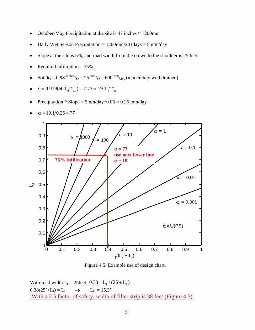
51

• October-May Precipitation at the site is 47 inches ≈ 1200mm

• Daily Wet Season Precipitation = 1200mm/241days = 5 mm/day

• Slope at the site is 5%, and road width from the crown to the shoulder is 25 feet.

• Required infiltration = 75%

•

•

Soil ks = 0.98 inches/hr = 25 mm/hr = 600 mm/day (moderately well drained)

λ = 0.019(600 dmm

ay ) + 7.73 = 19.1 dmm

ay

• Precipitation * Slope = 5mm/day*0.05 = 0.25 mm/day

• 19.1 0.25 77α = =

With road width Lr = 25feet, f f0.38 L / (25' L )= + 0.38(25’+Lf) = Lf → Lf = 15.3’ With a 2.5 factor of safety, width of filter strip is 38 feet (Figure 4.5).

Figure 4.5: Example use of design chart.

0 0.1 0.2 0.3 0.4 0.5 0.6 0.7 0.8 0.9 10

0.1

0.2

0.3

0.4

0.5

0.6

0.7

0.8

0.9

1

I %

Lf/(Lr + Lf)

α = 0.001

α = 0.01

α = 0.1

α = 10α = 100α = 1000

α=λ/(PS)

α = 1

75% Infiltration

α = 77 use next lower line α = 10

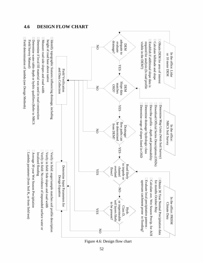
52

4.6 DESIGN FLOW CHART In the office: Lidar or 10 m

eter DEM

Field Verification

and Data C

ollection

DEM

adequate to evaluate

drainage?

In the office: N

RC

S Soil Survey

�D

etermine M

ap Units (W

eb Soil Survey)�

Dow

nload Official Series D

escriptions ( OSD

s)�

Describe profile – depth and perrm

eability�

Determ

ine drainage/ hydrologic class�

Determ

ine range of slopes listed in OSD

�O

btain DEM

for area of interest�

Calculate hillshade and slope

�Establish if additional slope data is required for analysis (Is road profile visible in the D

EM?)

�Identify topographic features influencing drainage, including height of road base above native

�M

easure road side slopes and road width

�D

etermine if local fill m

aterial was used in road construction

�D

etermine w

ater table depth or hydric qualifiers (Refer to N

RC

S Field Survey M

anual)�

Field determination of lam

bda (see Design M

ethods)

DEM

Slope data m

atches O

SD?

YES

Drainage/

flow paths can

be determined

from D

EM?

YES

Hydr.

Class D

, or im

permeable

soil layers likely to be present?

YES

YES

NO

Road likely

to impede or

channel overland flow

s ?

YES

NO

NO

Determ

ine Input Parameters for

Design Equation

�V

erify in field: auger/sample m

atches soil profile description �

Verify in field: Side slopes and road w

idth�

Verify in field: N

o evidence of impounded surface w

ater or localized flooding

�A

verage 30 year Wet Season Precipitation

�Lam

bda parameter (from

Soil Ks or from

field test)

NO

NO

In the office: PRISM

C

limate D

ata

�

Obtain 30 Y

ear Norm

al Precipitation data for m

onths October -M

ay�

Calculate ave. W

et Season Precip. for AO

I�

Evaluate local precipitation patterns -upstream

catchment prone to flooding?

Figure 4.6: Design flow chart

53

5.0 REFERENCES

Ahearn, D., and R. Tveten. Legacy LID: Stormwater Treatment in Unimproved Embankments along Highway Shoulders in Western Washington. Low Impact Development for Urban Ecosystem and Habitat Protection Conference, Seattle, WA, 2008. Arora, K., S.K. Mickelson, J.L. Baker, D.P. Tierney, and C.J. Peters. Herbicide Retention by Vegetative Buffer Strips from Runoff under Natural Rainfall. Transactions of the ASAE, Vol. 39, Issue 6, 1996, pp. 2155-2162. Barfield, B.J., R.L. Blevins, A.W. Flofle, C.E. Madison, S. Inamder, D.I. Carey, and V.P. Evangelou. Water Quality Impacts of Natural Riparian Grasses: Empirical Studies. St. Joseph, MI: American Society of Agricultural Engineers, No. 922100. ASAE Paper. 1992. Blanco-Canqui, H., C.J. Gantzer, S.H. Anderson, E.E. Alberts, and A.L. Thompson. Grass Barrier and Vegetative Filter Strip Effectiveness in Reducing Runoff, Sediment, Nitrogen, and Phosphorus Loss. Soil Science Society of America Journal, Vol. 68, No. 5, 2004, p. 1670. Bouchard, N.R., D.L. Osmond, R.J. Winston, and W.F. Hunt. The Capacity of Roadside Vegetated Filter Strips and Swales to Sequester Carbon. Ecological Engineering, Vol. 54, 2013, pp. 227-32. Buckingham, E. On Physically Similar Systems; Illustrations of the Use of Dimensional Equations. Physical Review, Vol. 4, Issue 4, 1914, p. 345. Cole, J.T., J.H. Baird, N.T. Basta, R.L. Huhnke, D.E. Storm, G.V. Johnson, M.E. Payton, M.D. Smolen, D.L. Martin, and J.C. Cole. Influence of Buffers on Pesticide and Nutrient Runoff from Bermuda grass Turf. Journal of Environment Quality, Vol. 26, No. 6, 1997, p. 1589. Davis, A.P., J.H. Stagge, E. Jamil, and H. Kim. Hydraulic performance of grass swales for managing highway runoff. Water Research, Vol. 46, Issue 20, 2012, pp.6775-6786. Diblasi, C.J., H. Li, A.P. Davis, and U. Ghosh. Removal and Fate of Polycyclic Aromatic Hydrocarbon Pollutants in an Urban Stormwater Bioretention Facility. Environmental Science & Technology, Vol.43, No. 2, 2009, pp. 494-502. Dillaha, T.A., R.B. Reneau, S. Mostaghimi, and D. Lee. Vegetative Filter Strips for Agricultural Nonpoint Source Pollution Control. Transactions of the ASAE, Vol. 32, Issue 2, 1989, pp. 513-519. Dosskey, M.G., M.J. Helmers, and D.E. Eisenhauer. A Design Aid for Determining Width of Filter Strips. Journal of Soil and Water Conservation, Vol. 63, No. 4, 2008, pp. 232-241.

54

Dosskey, M.G., K.D. Hoagland, and J.R. Brandle. Change in Filter Strip Performance Over Ten Years. Journal Soil and Water Conservation, Vol. 62, 2007, pp. 21-32. Doyle, R.C., G.C. Stanton, and D.C. Wolf. Effectiveness of Forest and Grass Buffer Strips in Improving Water Quality of Manure-Polluted Runoff. American Society of Agricultural Engineers, 1977, pp. 1-32. Fischer, R.A., and J.C. Fischenich. Design Recommendations for Riparian Corridors and Vegetated Buffer Strips. No. ERDC-TN-EMRRP-SR-24. Army Engineer Waterways Experiment Station Vicksburg MS. Engineer Research and Development Center, 2000. Fox, G.A., E.M. Matlock, J.A. Guzman, D. Sahoo, and K.B. Stunkel. Load Reduction from Runoff by Vegetative Filter Strips: A Laboratory-Scale Study. Journal of Environment Quality, Vol. 40, No. 3, 2011, p. 980. Gao, B., M.T. Walter, T.S. Steenhuis, J.Y. Parlange, B.K. Richards, W.L. Hogarth, and C.W. Rose. Investigating Raindrop Effects on Transport of Sediment and Non-sorbed Chemicals from Soil to Surface Runoff. Journal of Hydrology, Vol. 308, Issues1-4, 2005, pp. 313-320. Grismer, M.E. Vegetative Filter Strips for Nonpoint Pollution Control in Agriculture. UCANR Publications, 2006. Habib, E., W.F. Krajewski, and A. Kruger. Sampling Errors of Tipping-Bucket Rain Gauge Measurements. Journal of Hydrologic Engineering, Vol. 6, Issue 2, 2001, pp. 159-166. Hashim, G.M., C.A.A. Ciesiolka, W.A. Yusoff, A.W. Nafis, M.R. Mispan, C.W. Rose, and K.J. Coughlan. Soil Erosion Processes in Sloping Land in the East Coast of Peninsular Malaysia. Soil Technology, Vol. 8, No. 3, 1995, pp. 215-233. Hatt, B.E., T.D. Fletcher, and A. Deletic. Hydraulic and Pollutant Removal Performance of Fine Media Stormwater Filtration Systems. Environmental Science & Technology, Vol. 42, No.7, 2008, pp. 2535-2541. Hoffmann, C.C., C. Kjaergaard, J. Uusi-Kämppä, H.C. Hansen, and B. Kronvang. Phosphorus Retention in Riparian Buffers: Review of Their Efficiency. Journal of Environmental Quality, Vol. 38, No. 5, 2009, pp. 1942-1955. Hollis, G.E., and J.C. Ovenden. A Tipping Bucket Flowmeter for Roadside Gully Runoff. Hydrological Processes, Vol. 1, Issue 4, 1987, pp. 391-96. Horner, R.R., H. Lim, and S.J. Burges. Hydrologic Monitoring of the Seattle Ultra-Urban Stormwater Management Projects. Water Resources Series, Technical Report No. 170. Seattle, WA: Department of Civil and Environmental Engineering, 2002. Huang, J., X. Zhao, and P. Wu. Surface Runoff Volumes from Vegetated Slopes During Simulated Rainfall Events. Journal of Soil and Water Conservation, Vol. 68, No. 4, 2013, pp. 283-295.

55

Hudson, N.W. Field Measurement of Soil Erosion and Runoff. FAO Bulletin, 1993. Humphrey, M., J. Istok, J. Lee, J. Hevesi, and A. Flint. A New Method for Automated Dynamic Calibration of Tipping-Bucket Rain Gauges. Journal of Atmospheric and Oceanic Technology, Vol. 14, 1997, pp. 1513-1519. Kayhanian, M., C. Suverkropp, A. Ruby, and K. Tsay. Characterization and Prediction of Highway Runoff Constituent Event Mean Concentration. Journal of Environmental Management, Vol. 85, No. 2, 2007, pp. 279-95. Koelsch, R.K., J.C. Lorimor, and K.R. Mankin. Vegetative Treatment Systems For Management Of Open Lot Runoff: Review Of Literature. Applied Engineering in Agriculture, Vol. 22, No. 1, 2006, pp. 141-53. Line, D.E., and W. F. Hunt. Performance of a Bioretention Area and a Level Spreader-Grass Filter Strip at Two Highway Sites in North Carolina. Journal of Irrigation and Drainage Engineering, Vol. 135, No. 2, 2009, pp. 217-24. Liu, X., X. Zhang, and M. Zhang. Major Factors Influencing the Efficacy of Vegetated Buffers on Sediment Trapping: A Review and Analysis. Journal of Environmental Quality, Vol. 37, No. 5, 2008, pp. 1667-1674. Mayer, P.M., S.K. Reynolds, M.D. Mccutchen, and T.J. Canfield. Meta-Analysis of Nitrogen Removal in Riparian Buffers. Journal of Environmental Quality, Vol. 36, No. 4, 2007, pp. 1172-1180. Meals, D.W., and D.C. Braun. Demonstration of Methods to Reduce Runoff from Dairy Manure Application Sites, Journal of Environmental Quality, Vol. 35, 2006, pp. 1088-1100. Moore, M.T., E.R. Bennett, C.M. Cooper, S. Smith, F.D. Shields, C.D. Milam, and J.L. Farris. Transport and Fate of Atrazine and Lambda-cyhalothrin in an Agricultural Drainage Ditch in the Mississippi Delta, USA. Agriculture, Ecosystems & Environment, Vol. 87, No. 3, 2001, pp. 309-314. Muñoz-Carpena, R., G.A. Fox, and G.J. Sabbagh. Parameter Importance and Uncertainty in Predicting Runoff Pesticide Reduction with Filter Strips. Journal of Environmental Quality, Vol. 39, No. 2, 2010, pp. 630-641. Nehls, T., Y.N. Rim, and G. Wessolek. Technical Note on Measuring Run-Off Dynamics from Pavements Using a New Device: The Weighable Tipping Bucket. Hydrolrology and Earth System Sciences, Vol. 15, 2011, pp. 1379-1386. Newberry, G.P., and D.R. Yonge. The Retardation of Heavy Metals in Stormwater Runoff by Highway Grass Strips. Rep. no. WA-RD-404.1. Pullman, WA: Washington State Department of Transportation, 1996.

56

Nystuen, J.A. Relative Performance of Automatic Rain Gauges Under Different Rainfall Conditions, Journal of Atmospheric and Oceanic Technology, Vol. 16, 1999, pp. 1025-1043. Nystuen, J.A., J.R. Proni, P.G. Black, and J.C. Wilkerson. A Comparison of Automatic Rain Gauges. Journal of Atmospheric and Oceanic Technology, Vol. 13, 1996, pp. 62-73. Parsons, J.E., R.B. Daniel, J.W. Gilliam, and T.A. Dillaha. Proceedings of the Conference on Environmentally Sound Agriculture: What Can Be Done Now? Publication. 1st ed. Vol. 1. Orlando, FL: Service and the Institute, 1991. Proceedings of the Conference on Environmentally. The Effect of Vegetation Filter Strips on Sediment and Nutrient Removal from Agricultural Runoff April 16-18. p. 324-332. Patty, L., B. Réal, and J. Joël Gril. The Use of Grassed Buffer Strips to Remove Pesticides, Nitrate and Soluble Phosphorus Compounds from Runoff Water. Pesticide Science, Vol. 49, Issue 3, 1997, pp. 243-251. Piguet, P., A. Parriaux, and M. Bensimon. The Diffuse Infiltration of Road Runoff: An Environmental Improvement. Science of the Total Environment, Vol. 397, Issues1-3, 2008, pp. 13-23. Pinson, W., D. Yoder, J. Buchanan, W. Wright, and J. Wilkerson. Design and Evaluation of an Improved Flow Divider for Sampling Runoff Plots. Applied Engineering in Agriculture, Vol. 20, No. 4, 2004, pp. 433-438. Poletika, N.N., P.N. Coody, G.A. Fox, G.J. Sabbagh, S.C. Dolder, and J. White. Chlorpyrifos and Atrazine Removal from Runoff by Vegetated Filter Strips: Experiments and Predictive Modeling. Journal of Environmental Quality, Vol. 38, No.3, 2009, pp. 1042-1052. PRISM Climate Group. Gridded Precipitation Data for Oregon. Oregon State University, http://prism.oregonstate.edu. Accessed November 7, 2013. Radatz, T.F., A.M. Thompson, and F.W. Madison. Soil Moisture and Rainfall Intensity Thresholds for Runoff Generation in Southwestern Wisconsin Agricultural Watersheds. Hydrological Processes, Vol. 27, Issue 25, 2013, pp. 3521-3534. Reister, M., and D. Yonge. Application of a Simplified Analysis Method for Natural Dispersion of Highway Stormwater Runoff. Rep. No. 618.1. Pullman, WA: Washington State Department of Transportation, 2005. Low Impact Stormwater Treatment Methods. Reister, M., and F. Fiedler. Simplified Analysis Method for Natural Dispersion of Highway Storm Water Runoff in Rural Areas. In Transportation Research Record: Journal of the Transportation Research Board, No. 1983, Transportation Research Board of the National Academies, Washington, D.C., 2006, pp. 33-41. Schmitt, T.J., M.G. Dosskey, and K.D. Hoagland. Filter Strip Performance and Processes for Different Vegetation, Widths, and Contaminants. Journal of Environmental Quality, Vol. 28, No. 5, 1999, pp. 1479-1489.

57

Shields, A. Anwendung der Aehnlichkeitsmechanik und der Turbulenzforschung auf die Geschiebebewegung. Preussischen Versuchsanstalt für Wasserbau, 1936. Srinivasan, M., M. Wittman, J. Hamlett, and W. Gburek. Surface and Subsurface Sensors to Record Variable Runoff Generation Areas, Transactions of the ASAE, Vol. 43, 2000, pp. 651-660. Stagge, J.H., A.P. Davis, E. Jamil, and H. Kim. Performance of Grass Swales for Improving Water Quality from Highway Runoff. Water Research, Vol. 46, No. 20, 2012, pp. 6731-6742. Stewart, R.D., R. Hut, D.E. Rupp, H. Gupta, and J.S. Selker. A Resonating Rainfall and Evaporation Recorder. Water Resources Research, Vol. 48, Issue 8, 2012. Stewart, R.D., Z. Liu, D.E. Rupp, C.W. Higgins, and J.S. Selker. A New Instrument to Measure Plot-Scale Runoff. Geoscientific Instrumentation, Methods and Data Systems, Vol. 4, No. 1, 2015, p. 57. Storey, B.J., M-H. Li, J.A. McFalls, and Y-J. Yi. Stormwater Treatment with Vegetated Buffers. Texas Transportation Institute, The Texas A&M University System, College Station, TX, 2009. Stomph, T., N. De Ridder, and N. Van de Giesen. A Flowmeter for Low Discharges of Laboratory Flumes, Transactions of the ASAE, Vol. 45, 2002, pp. 345-349. USDA, NRCS, Soil Survey Staff. Soil Survey Manual, 1993. USDA, NRCS. National Soil Survey Handbook, Title 430-VI, 2002. USDA, NRCS, Soil Survey Staff. Web Soil Survey. 2003. Available online at http://websoilsurvey.nrcs.usda.gov/. Accessed February 2014 to November 2015. US EPA. Riparian Buffer Width, Vegetative Cover, and Nitrogen Removal Effectiveness: A Review of Current Science and Regulations. By P. M. Mayer, S. Reynolds, T. Canfield, and M. McCutchen. Washington, DC: n.p., 2005. EPA/600/R-05/118. Winston, R.J., W.F. Hunt, D.L. Osmond, W.G. Lord, and M.D. Woodward. Field Evaluation of Four Level Spreader–Vegetative Filter Strips to Improve Urban Storm-Water Quality. Journal of Irrigation and Drainage Engineering, Vol. 137, No. 3, 2011, pp. 170-82. Winston, R.J., W.F. Hunt, S.G. Kennedy, J. D. Wright, and M.S. Lauffer. Field Evaluation of Storm-Water Control Measures for Highway Runoff Treatment. Journal of Environmental Engineering, Vol. 138, No. 1, 2012, pp. 101-11. Young, R.A., T. Huntrods, and W. Anderson. Effectiveness of Vegetated Buffer Strips in Controlling Pollution from Feedlot Runoff. Journal of Environmental Quality, Vol. 9, No. 3, 1980, pp. 483-487.

58

Yu, B., C.W. Rose, K. Coughlan, and B. Fentie. Plot-Scale Rainfall-Runoff Characteristics and Modeling at Six Sites in Australia and Southeast Asia. Transactions of the ASAE, Vol. 40, 1997, pp. 1295-1303. Yu, C., B. Gao, and R. Muñoz-Carpena. Effect of Dense Vegetation on Colloid Transport and Removal in Surface Runoff. Journal of Hydrology, Vol. 434-435, 2012, pp. 1-6. Yu, C., B. Gao, R. Muñoz-Carpena, Y. Tian, L. Wu, and O. Perez-Ovilla. A Laboratory Study of Colloid and Solute Transport in Surface Runoff on Saturated Soil. Journal of Hydrology, Vol. 402, Issues 1-2, 2011, pp. 159-64. Yu, C., R. Muñoz-Carpena, B. Gao, and O. Perez-Ovilla. Effects of Ionic Strength, Particle Size, Flow Rate, and Vegetation Type on Colloid Transport through a Dense Vegetation Saturated Soil System: Experiments and Modeling. Journal of Hydrology, Vol. 499, 2013, pp. 316-23. Yuan, Y., R.L. Bingner, and M.A. Locke. A Review of Effectiveness of Vegetative Buffers on Sediment Trapping in Agricultural Areas. Ecohydrology, Vol. 2, Issue 3, 2009, pp. 321-36. Zhao, S., E. Dorsey, S. Gupta, J. Moncrief, and D. Huggins. Automated Water Sampling and Flow Measuring Devices for Runoff and Subsurface Drainage. Journal of Soil and Water Conservation, Vol. 56, No. 4, 2001, pp. 299-306.

APPENDIX A MAPS OF MONITORING SITES

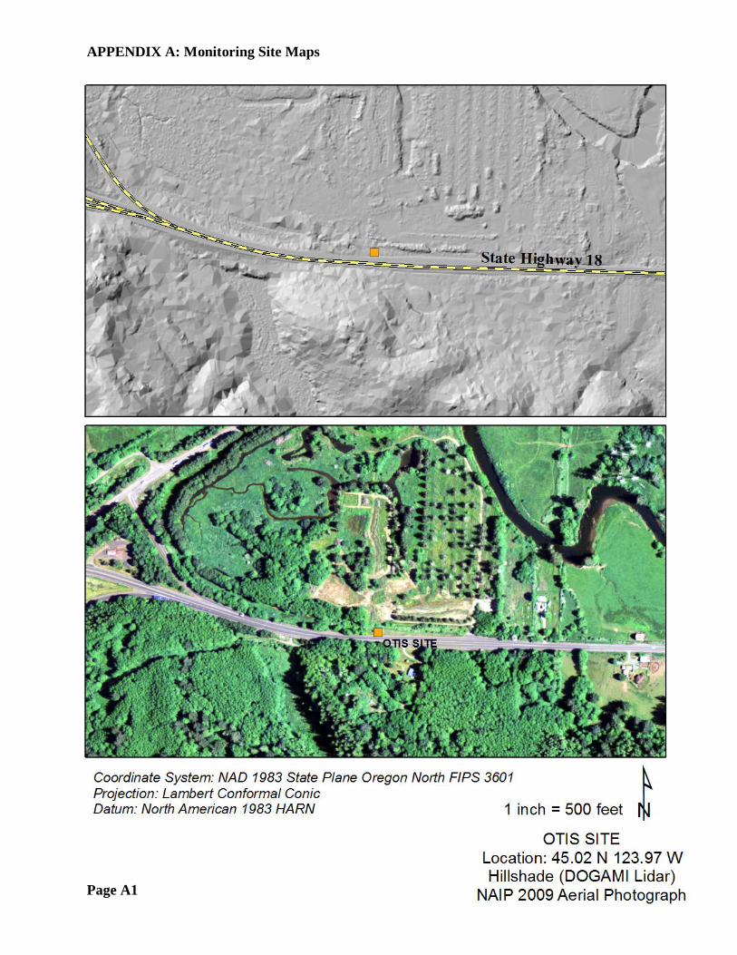
APPENDIX A: Monitoring Site Maps

Page A1

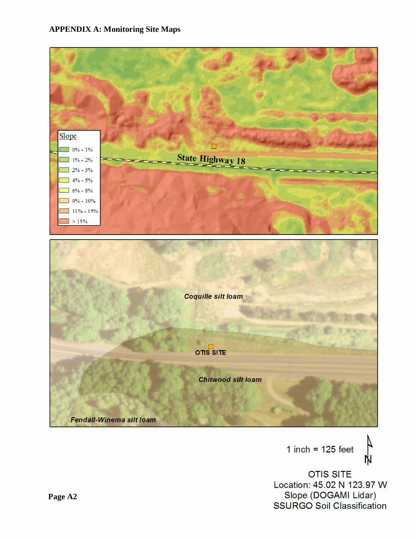
APPENDIX A: Monitoring Site Maps

Page A2

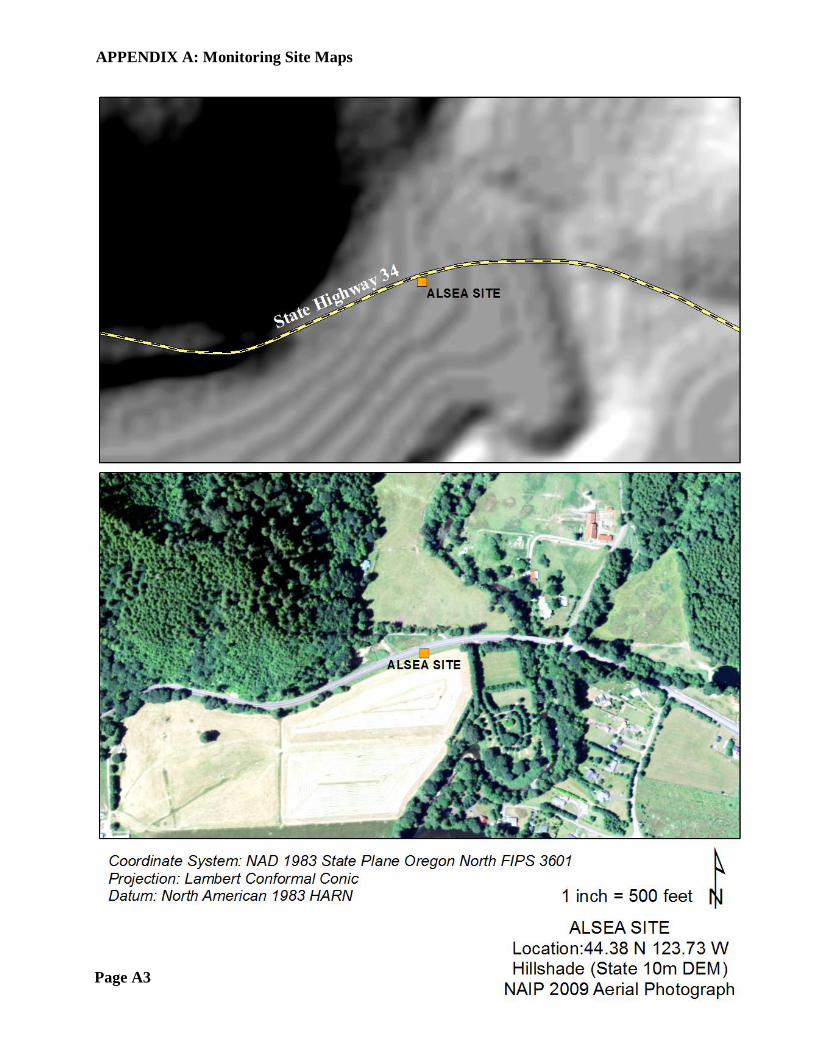
APPENDIX A: Monitoring Site Maps

Page A3

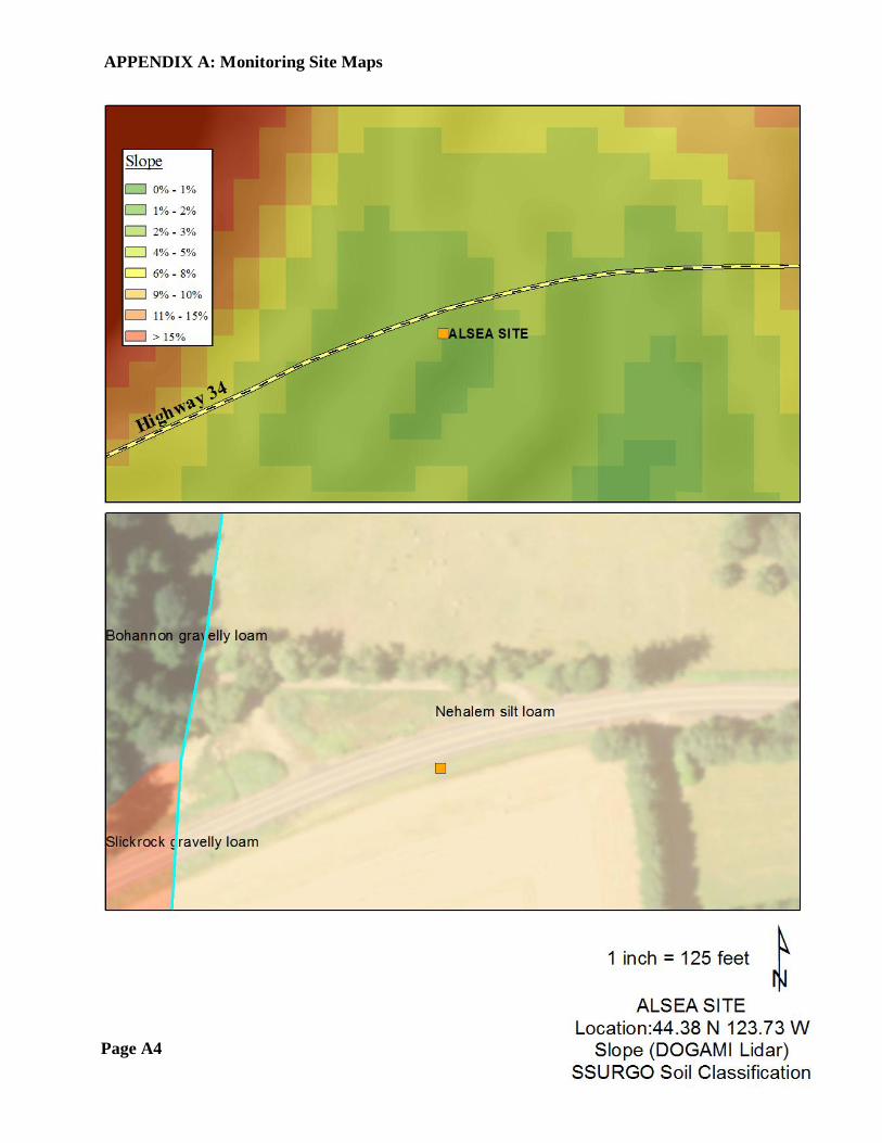
APPENDIX A: Monitoring Site Maps

Page A4

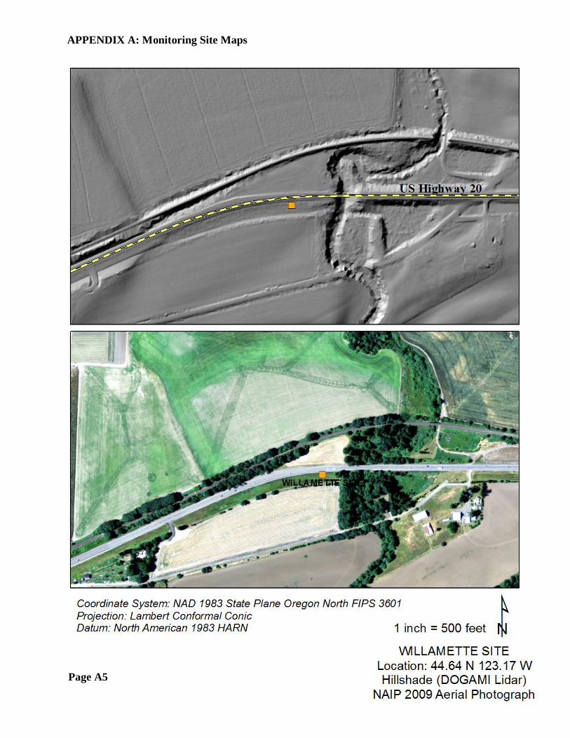
APPENDIX A: Monitoring Site Maps

Page A5

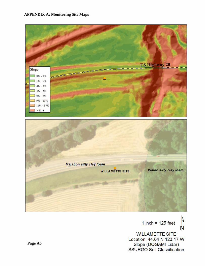
APPENDIX A: Monitoring Site Maps

Page A6

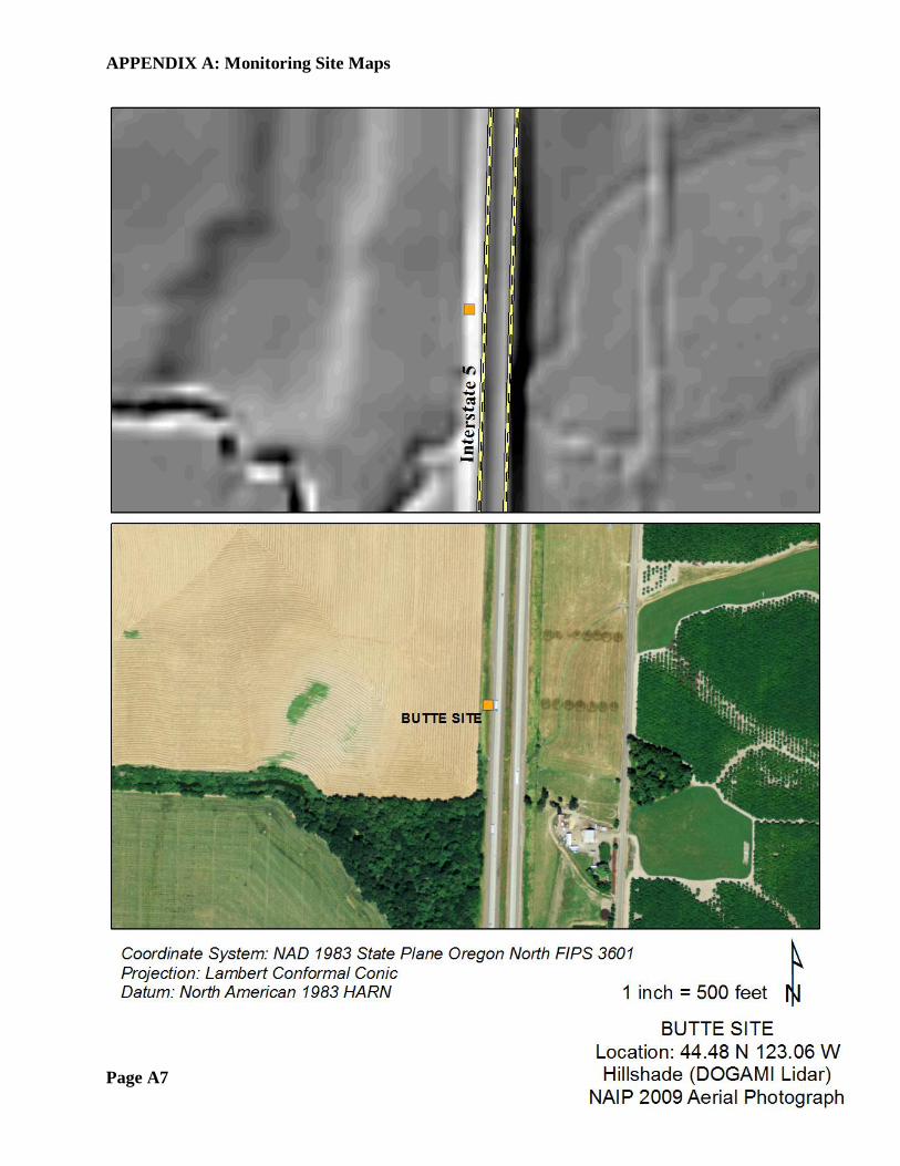
APPENDIX A: Monitoring Site Maps

Page A7

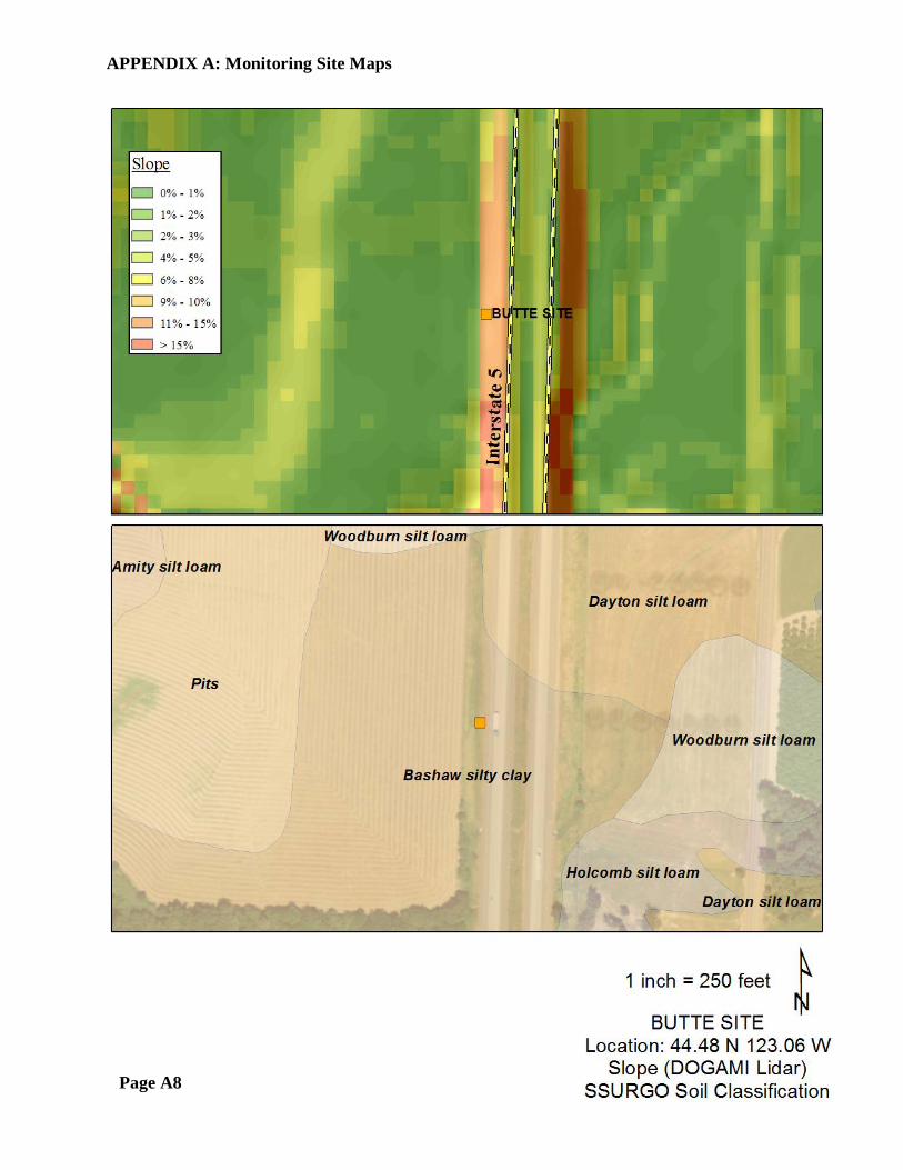
APPENDIX A: Monitoring Site Maps

Page A8

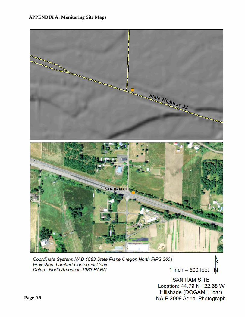
APPENDIX A: Monitoring Site Maps

Page A9

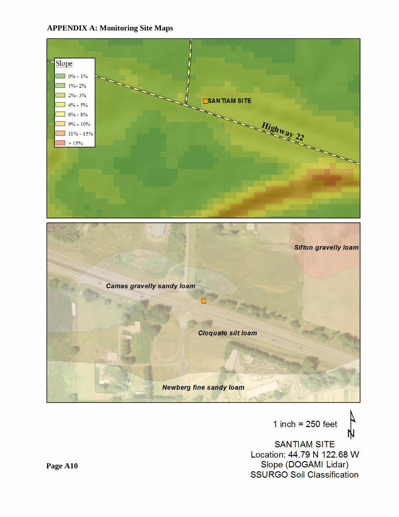
APPENDIX A: Monitoring Site Maps

Page A10

APPENDIX B ODOT ISSUED PERMITS FOR FILED SITES

APPENDIX C SUMMARY OF INFILTRATION TEST RESULTS

C1

Appendix C – Infiltration Tests and Analysis

We measured infiltration rates at the five sites using single ring infiltration tests (Table 1). The infiltration rings had 4.8 cm diameters, and during measurements were inserted into the soil approximately 1 cm. To conduct an infiltration test, water was added to the ring in 100 mL increments; the time for each increment to fully infiltrate was measured with a stopwatch and recorded. Up to 1400 mL were added in total. Due to the high spatial variability of infiltration rates, during each sampling event we performed between 9 and 18 discrete infiltration tests per site, of which a minimum of 6 were determined to be valid via subsequent analysis (Table 1).

We analyzed the infiltration test data using the two-term Philip infiltration model rewritten in the general form suggested by Smiles and Knight [1976]:

2/12/1 CtS

tI

+= (1)

where I is the cumulative infiltration, S is the soil sorptivity, C is a constant, and t is the elapsed time. In our analysis, we determined S and C as the respective intercept and slope of a linear model fit to infiltration data (i.e., I/t1/2 as a function of t1/2). In some cases, the intercept of the regression line (i.e., S) or the slope of the regression line (i.e., C) was determined to be negative; given that this is a non-physical result, such tests were excluded from further analysis. In total, 34 tests out of 175 were removed for this reason.

Table 1 – Location, dates, and number of tests (rings) for each infiltration test.

Site Name Highway Sampling Dates

Number of Valid Tests*

Alsea OR-34 2013-09-17 8

2014-01-17 9

2014-07-10 6

Butte I-5 2013-09-04 7

2013-09-19 8

2014-06-30 7

Otis OR-18 2013-08-28 18

2014-07-08 6

Santiam OR-22 2013-09-11 14

2014-01-22 13

2014-07-13 12

Willamette OR-20 2013-09-12 9

2014-01-23 8

2014-07-22 7

2014-07-24 9

*Valid tests refer to tests where the regression analysis on Equation (1) produced positive values for both S and C.

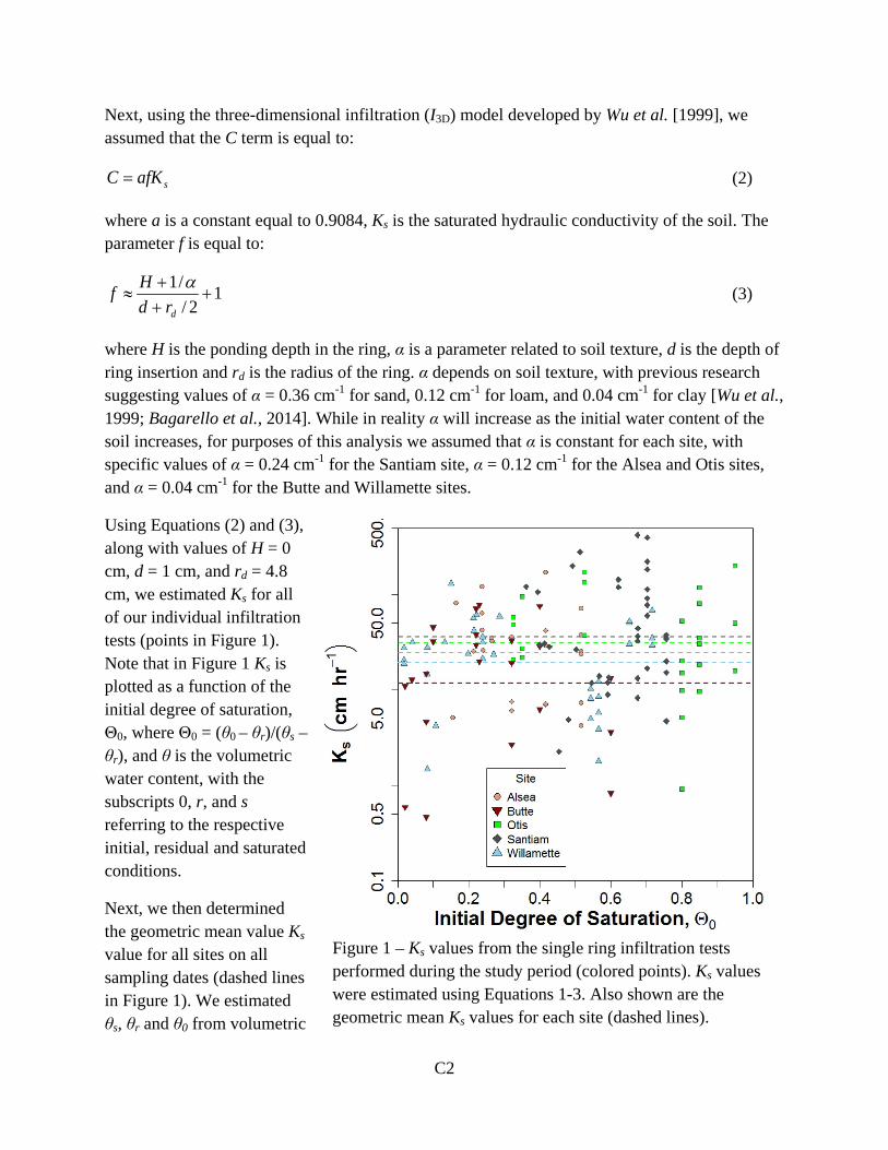
C2

Next, using the three-dimensional infiltration (I3D) model developed by Wu et al. [1999], we assumed that the C term is equal to:

safKC = (2)

where a is a constant equal to 0.9084, Ks is the saturated hydraulic conductivity of the soil. The parameter f is equal to:

12/

/1+

++

≈drd

Hf α (3)

where H is the ponding depth in the ring, α is a parameter related to soil texture, d is the depth of ring insertion and rd is the radius of the ring. α depends on soil texture, with previous research suggesting values of α = 0.36 cm-1 for sand, 0.12 cm-1 for loam, and 0.04 cm-1 for clay [Wu et al., 1999; Bagarello et al., 2014]. While in reality α will increase as the initial water content of the soil increases, for purposes of this analysis we assumed that α is constant for each site, with specific values of α = 0.24 cm-1 for the Santiam site, α = 0.12 cm-1 for the Alsea and Otis sites, and α = 0.04 cm-1 for the Butte and Willamette sites.

Using Equations (2) and (3), along with values of H = 0 cm, d = 1 cm, and rd = 4.8 cm, we estimated Ks for all of our individual infiltration tests (points in Figure 1). Note that in Figure 1 Ks is plotted as a function of the initial degree of saturation, Θ0, where Θ0 = (θ0 – θr)/(θs – θr), and θ is the volumetric water content, with the subscripts 0, r, and s referring to the respective initial, residual and saturated conditions.

Next, we then determined the geometric mean value Ks value for all sites on all sampling dates (dashed lines in Figure 1). We estimated θs, θr and θ0 from volumetric

Figure 1 – Ks values from the single ring infiltration tests performed during the study period (colored points). Ks values were estimated using Equations 1-3. Also shown are the geometric mean Ks values for each site (dashed lines).

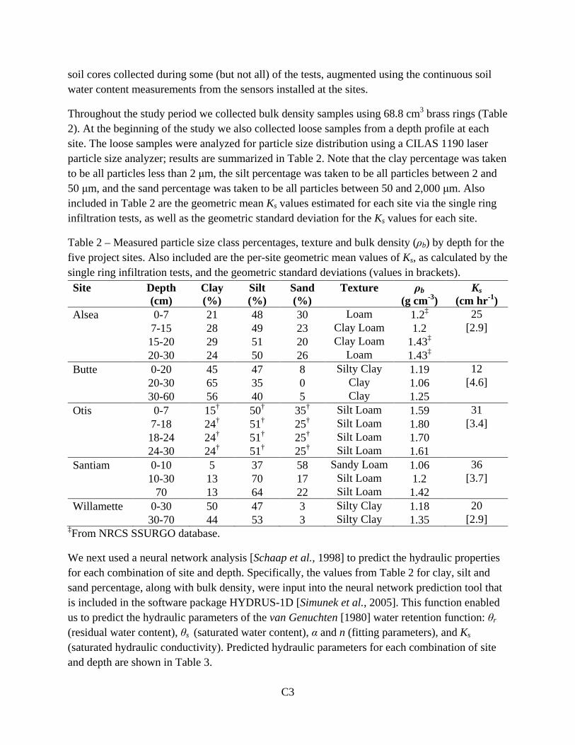
C3

soil cores collected during some (but not all) of the tests, augmented using the continuous soil water content measurements from the sensors installed at the sites.

Throughout the study period we collected bulk density samples using 68.8 cm3 brass rings (Table 2). At the beginning of the study we also collected loose samples from a depth profile at each site. The loose samples were analyzed for particle size distribution using a CILAS 1190 laser particle size analyzer; results are summarized in Table 2. Note that the clay percentage was taken to be all particles less than 2 μm, the silt percentage was taken to be all particles between 2 and 50 μm, and the sand percentage was taken to be all particles between 50 and 2,000 μm. Also included in Table 2 are the geometric mean Ks values estimated for each site via the single ring infiltration tests, as well as the geometric standard deviation for the Ks values for each site.

Table 2 – Measured particle size class percentages, texture and bulk density (ρb) by depth for the five project sites. Also included are the per-site geometric mean values of Ks, as calculated by the single ring infiltration tests, and the geometric standard deviations (values in brackets). Site Depth

(cm) Clay (%)

Silt (%)

Sand (%)

Texture ρb (g cm-3)

Ks (cm hr-1)

Alsea 0-7 21 48 30 Loam 1.2‡ 25

7-15 28 49 23 Clay Loam 1.2 [2.9]

15-20 29 51 20 Clay Loam 1.43‡ 20-30 24 50 26 Loam 1.43‡ Butte 0-20 45 47 8 Silty Clay 1.19 12

20-30 65 35 0 Clay 1.06 [4.6]

30-60 56 40 5 Clay 1.25 Otis 0-7 15† 50† 35† Silt Loam 1.59 31 7-18 24† 51† 25† Silt Loam 1.80 [3.4] 18-24 24† 51† 25† Silt Loam 1.70 24-30 24† 51† 25† Silt Loam 1.61 Santiam 0-10 5 37 58 Sandy Loam 1.06 36

10-30 13 70 17 Silt Loam 1.2 [3.7]

70 13 64 22 Silt Loam 1.42 Willamette 0-30 50 47 3 Silty Clay 1.18 20 30-70 44 53 3 Silty Clay 1.35 [2.9]

‡From NRCS SSURGO database.

We next used a neural network analysis [Schaap et al., 1998] to predict the hydraulic properties for each combination of site and depth. Specifically, the values from Table 2 for clay, silt and sand percentage, along with bulk density, were input into the neural network prediction tool that is included in the software package HYDRUS-1D [Simunek et al., 2005]. This function enabled us to predict the hydraulic parameters of the van Genuchten [1980] water retention function: θr (residual water content), θs (saturated water content), α and n (fitting parameters), and Ks (saturated hydraulic conductivity). Predicted hydraulic parameters for each combination of site and depth are shown in Table 3.

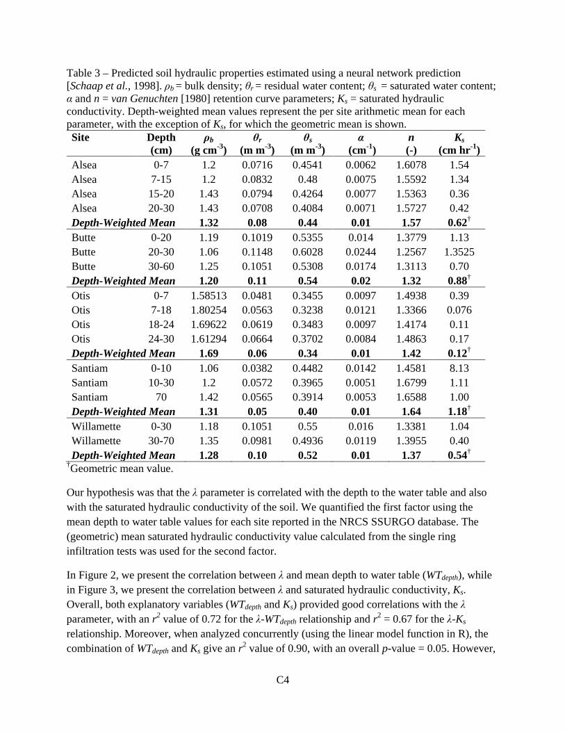
C4

Table 3 – Predicted soil hydraulic properties estimated using a neural network prediction [Schaap et al., 1998]. ρb = bulk density; θr = residual water content; θs = saturated water content; α and n = van Genuchten [1980] retention curve parameters; Ks = saturated hydraulic conductivity. Depth-weighted mean values represent the per site arithmetic mean for each parameter, with the exception of Ks, for which the geometric mean is shown. Site Depth

(cm) ρb

(g cm-3) θr

(m m-3) θs

(m m-3) α

(cm-1) n (-)

Ks (cm hr-1)

Alsea 0-7 1.2 0.0716 0.4541 0.0062 1.6078 1.54 Alsea 7-15 1.2 0.0832 0.48 0.0075 1.5592 1.34 Alsea 15-20 1.43 0.0794 0.4264 0.0077 1.5363 0.36 Alsea 20-30 1.43 0.0708 0.4084 0.0071 1.5727 0.42 Depth-Weighted Mean 1.32 0.08 0.44 0.01 1.57 0.62† Butte 0-20 1.19 0.1019 0.5355 0.014 1.3779 1.13 Butte 20-30 1.06 0.1148 0.6028 0.0244 1.2567 1.3525 Butte 30-60 1.25 0.1051 0.5308 0.0174 1.3113 0.70 Depth-Weighted Mean 1.20 0.11 0.54 0.02 1.32 0.88† Otis 0-7 1.58513 0.0481 0.3455 0.0097 1.4938 0.39 Otis 7-18 1.80254 0.0563 0.3238 0.0121 1.3366 0.076 Otis 18-24 1.69622 0.0619 0.3483 0.0097 1.4174 0.11 Otis 24-30 1.61294 0.0664 0.3702 0.0084 1.4863 0.17 Depth-Weighted Mean 1.69 0.06 0.34 0.01 1.42 0.12† Santiam 0-10 1.06 0.0382 0.4482 0.0142 1.4581 8.13 Santiam 10-30 1.2 0.0572 0.3965 0.0051 1.6799 1.11 Santiam 70 1.42 0.0565 0.3914 0.0053 1.6588 1.00 Depth-Weighted Mean 1.31 0.05 0.40 0.01 1.64 1.18† Willamette 0-30 1.18 0.1051 0.55 0.016 1.3381 1.04 Willamette 30-70 1.35 0.0981 0.4936 0.0119 1.3955 0.40 Depth-Weighted Mean 1.28 0.10 0.52 0.01 1.37 0.54†

†Geometric mean value.

Our hypothesis was that the λ parameter is correlated with the depth to the water table and also with the saturated hydraulic conductivity of the soil. We quantified the first factor using the mean depth to water table values for each site reported in the NRCS SSURGO database. The (geometric) mean saturated hydraulic conductivity value calculated from the single ring infiltration tests was used for the second factor.

In Figure 2, we present the correlation between λ and mean depth to water table (WTdepth), while in Figure 3, we present the correlation between λ and saturated hydraulic conductivity, Ks. Overall, both explanatory variables (WTdepth and Ks) provided good correlations with the λ parameter, with an r2 value of 0.72 for the λ-WTdepth relationship and r2 = 0.67 for the λ-Ks relationship. Moreover, when analyzed concurrently (using the linear model function in R), the combination of WTdepth and Ks give an r2 value of 0.90, with an overall p-value = 0.05. However,

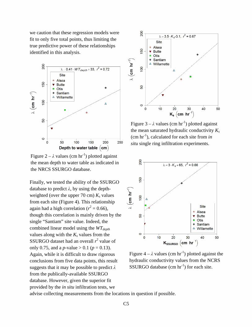
C5

we caution that these regression models were fit to only five total points, thus limiting the true predictive power of these relationships identified in this analysis.

Finally, we tested the ability of the SSURGO database to predict λ, by using the depth-weighted (over the upper 70 cm) Ks values from each site (Figure 4). This relationship again had a high correlation (r2 = 0.66), though this correlation is mainly driven by the single “Santiam” site value. Indeed, the combined linear model using the WTdepth values along with the Ks values from the SSURGO dataset had an overall r2 value of only 0.75, and a p-value > 0.1 (p = 0.13). Again, while it is difficult to draw rigorous conclusions from five data points, this result suggests that it may be possible to predict λ from the publically-available SSURGO database. However, given the superior fit provided by the in situ infiltration tests, we advise collecting measurements from the locations in question if possible.

Figure 2 – λ values (cm hr-1) plotted against the mean depth to water table as indicated in the NRCS SSURGO database.

Figure 3 – λ values (cm hr-1) plotted against the mean saturated hydraulic conductivity Ks (cm hr-1), calculated for each site from in situ single ring infiltration experiments.

Figure 4 – λ values (cm hr-1) plotted against the hydraulic conductivity values from the NCRS SSURGO database (cm hr-1) for each site.

C6

References

Assouline, S., and D. Or (2014), The concept of field capacity revisited: Defining intrinsic static and dynamic criteria for soil internal drainage dynamics, Water Resour. Res., n/a-n/a.

Bagarello, V., S. Di Prima, M. Iovino, and G. Provenzano (2014), Estimating field-saturated soil hydraulic conductivity by a simplified Beerkan infiltration experiment, Hydrol. Processes, 28(3), 1095-1103.

Schaap, M. G., F. J. Leij, and M. T. van Genuchten (1998), Neural network analysis for hierarchical prediction of soil hydraulic properties, Soil Sci. Soc. Am. J., 62(4), 847-855.

Simunek, J., M. T. Van Genuchten, and M. Sejna (2005), The HYDRUS-1D software package for simulating the one-dimensional movement of water, heat, and multiple solutes in variably-saturated media, University of California, Riverside, Research reports, 240.

Smiles, D. E., and J. H. Knight (1976), A note on the use of the Philip infiltration equation, Soil Res., 14(1), 103-108.

van Genuchten, M. T. (1980), A closed-form equation for predicting the hydraulic conductivity of unsaturated soils, Soil Sci. Soc. Am. J., 44(5), 892-898.

Wu, L., L. Pan, J. Mitchell, and B. Sanden (1999), Measuring saturated hydraulic conductivity using a generalized solution for single-ring infiltrometers, Soil Sci. Soc. Am. J., 63(4), 788-792.

APPENDIX D EXAMPLE SOIL SERIES DESCRIPTIONS USED IN DESIGN

EQUATIONS

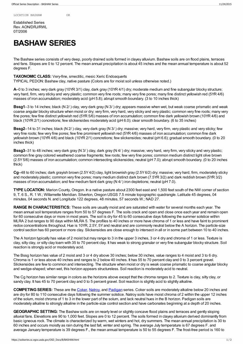
LOCATION BASHAW OR

Established SeriesRev. AON/DRJ/RWL07/2006

BASHAW SERIES

The Bashaw series consists of very deep, poorly drained soils formed in clayey alluvium. Bashaw soils are on flood plains, terracesand fans. Slopes are 0 to 12 percent. The mean annual precipitation is about 45 inches and the mean annual temperature is about 52degrees F.

TAXONOMIC CLASS: Very-fine, smectitic, mesic Xeric Endoaquerts TYPICAL PEDON: Bashaw clay, native pasture (Colors are for moist soil unless otherwise noted.)

A--0 to 3 inches; very dark gray (10YR 3/1) clay, dark gray (10YR 4/1) dry; moderate medium and fine subangular blocky structure;very hard, firm, very sticky and very plastic; common very fine roots; many very fine pores; many fine distinct yellowish red (5YR 4/6)masses of iron accumulation; moderately acid (pH 5.8); abrupt smooth boundary. (3 to 10 inches thick)

Bssg1--3 to 14 inches; black (N 2/ ) clay, very dark gray (N 3/ ) dry; appears massive when wet, but weak coarse prismatic and weakcoarse angular blocky structure when moist or dry; very firm, very hard, very sticky and very plastic; common very fine roots; many veryfine pores; few fine distinct yellowish red (5YR 5/6) masses of iron accumulation; common fine dark yellowish brown (10YR 4/6) andblack (10YR 2/1) concretions; few slickensides moderately acid (pH 6.0); clear smooth boundary. (6 to 35 inches)

Bssg2--14 to 31 inches; black (N 2/ ) clay, very dark gray (N 3/ ) dry; massive; very hard, very firm, very plastic and very sticky; fewvery fine roots; few very fine pores; few fine prominent yellowish red (5YR 4/6) masses of iron accumulation; common fine darkyellowish brown (10YR 4/6) and black (10YR 2/1) concretions; few slickensides; neutral (pH 6.6); gradual smooth boundary. (0 to 20inches thick)

Bssg3--31 to 48 inches; very dark gray (N 3/ ) clay, dark gray (N 4/ ) dry; massive; very hard, very firm, very sticky and very plastic;common fine gray colored weathered coarse fragments; few roots; few very fine pores; common medium distinct light olive brown(2.5Y 5/6) masses of iron accumulation; common intersecting slickensides; neutral (pH 7.0); abrupt smooth boundary. (0 to 20 inchesthick)

Cg--48 to 60 inches; dark grayish brown (2.5Y 4/2) clay, light brownish gray (2.5Y 6/2) dry; massive; very hard, firm, moderately stickyand moderately plastic; common very fine pores; many medium distinct dark brown (7.5YR 3/2) and dark reddish brown (5YR 3/2)masses of iron accumulation; and few medium faint dark gray (N 4/ ) iron depletions; neutral (pH 7.0).

TYPE LOCATION: Marion County, Oregon. In a native pasture about 2300 feet east and 1,500 feet south of the NW corner of section9, T. 6 S., R. 1 W.; Willamette Meridian. Silverton, Oregon USGS 7.5 minute topographic quadrangle. Latitude 45 degrees, 04minutes, 04 seconds N. and Longitude 122 degrees, 48 minutes, 57 seconds W.; NAD 27.

RANGE IN CHARACTERISTICS: These soils are usually moist and are saturated with water for several months each year. Themean annual soil temperature ranges from 50 to 57 degrees F. The soils crack and open and close once each year and remain openfor 60 consecutive days or more in most years. The soil is dry for 45 to 60 consecutive days following the summer solstice withinMLRA 2 but ranges to 90 days within MLRA 5. The profiles to 40 inches or more have chroma of 1 or less and have faint to prominentredox concentrations throughout. Hue is 10YR, 2.5Y, 5Y and neutral and are commonly neutral below the A horizon. The particle-sizecontrol section has 60 percent or more clay. Slickensides are close enough to intersect in all or in some part between 10 to 40 inches.

The A horizon typically has value of 2 moist but may range to 3 in the upper 3 inches, 3 or 4 dry and chroma of 1 or less. Texture isclay, silty clay, or silty clay loam with 35 to 70 percent clay. It has weak to strong granular or very fine subangular blocky structure. Soilreaction is strongly acid or moderately acid.

The Bssg horizon has value of 2 moist and 3 or 4 dry above 30 inches; below 30 inches, value ranges to 4 moist and 3 to 6 dry.Chroma is 1 or less above 40 inches and ranges to 2 below 40 inches. It has 55 to 70 percent clay and 0 to 3 percent gravel.Slickensides are few to common and intersecting. The structure when moist or dry is weak coarse prismatic to coarse angular blockyand wedge-shaped; when wet, this horizon appears structureless. Soil reaction is moderately acid to neutral.

The Cg horizon has similar range in colors as the horizons above except that the chroma ranges to 2. Texture is clay, silty clay, orsandy clay. It has 45 to 70 percent clay and 0 to 5 percent gravel. Soil reaction is slightly acid to slightly alkaline.

COMPETING SERIES: These are the Coker, Natroy, and Padigan series. Coker soils are moderately alkaline below 20 inches andare dry for 80 to 110 consecutive days following the summer solstice. Natroy soils have moist chroma of 2 within the upper 12 inchesof the solum, moist chroma of 1 to 3 in the lower part of the solum, and lack neutral hues in the B horizon. Padigan soils aremoderately alkaline to strongly alkaline in the particle-size control section and have carbonates beginning at a depth of 20 inches.

GEOGRAPHIC SETTING: The Bashaw soils are on nearly level or slightly concave flood plains and terraces and gently slopingalluvial fans. Elevations are 90 to 1,000 feet. Slopes are 0 to 12 percent. The soils formed in clayey alluvium derived dominantly frombasic igneous rock. The climate is characterized by warm, wet winters and hot, dry summers. The mean annual precipitation is 30 to60 inches and occurs moistly as rain during the last fall, winter and spring. The average July temperature is 67 degrees F. andaverage January temperature is 39 degrees F., the mean annual temperature is 50 to 55 degrees F. The frost-free period is 160 to

Official Series Description - BASHAW Series 11/24/2015

https://soilseries.sc.egov.usda.gov/OSD_Docs/B/BASHAW.html 1 / 2

235 days.

GEOGRAPHICALLY ASSOCIATED SOILS: These are the Cove, Waldo, Wapato and Witham soils. All of these soils lackintersecting slickensides. In addition, Wapato soils are moderately fine textured with less than 35 percent clay and the Witham soilsare somewhat poorly drained. Cove soils are on flood plains and terraces in areas that alluvium is from mixed sources. Waldo andWapato soils are on flood plains adjacent to the river or stream. Witham soils are on fans, foot slopes, and toe slopes.

DRAINAGE AND PERMEABILITY: Poorly drained; very slow permeability. An apparent water table is at its uppermost limit fromNovember to May and is ponded from December to April. Where this soil occurs on flood plains, occasional or frequent flooding forlong periods occurs from December to April unless protected.

USE AND VEGETATION: These soils are used for pasture and for growing spring grains. Natural vegetation is sedges, rushes,grasses, scattered ash, willows and other trees and shrubs.

DISTRIBUTION AND EXTENT: Willamette Valley in western Oregon; MLRA 2, 5. The soils occur in small bodies and areinextensive.

MLRA SOIL SURVEY REGIONAL OFFICE (MO) RESPONSIBLE: Portland, Oregon

SERIES ESTABLISHED: Benton County (Benton Area), Oregon, 1970.

REMARKS: Diagnostic features recognized in this pedon:

Aquerts feature - the zone from 0 to 48 inches having aquic conditions for sometime in most years and chroma of 1 or less with redoxconcentrations.Endosaturation - the zone from 0 to 60 inches is saturated with water for some period of time.

The classification was changed from Typic Pelloxererts to Xeric Endoaquerts in 5/94.

ADDITIONAL DATA: Characterization data is available for sample #S99OR-043-001, S96OR-043-003, and S92OR-003-004NSSL, Lincoln, NE, 12/01.

National Cooperative Soil SurveyU.S.A.

Official Series Description - BASHAW Series 11/24/2015

https://soilseries.sc.egov.usda.gov/OSD_Docs/B/BASHAW.html 2 / 2

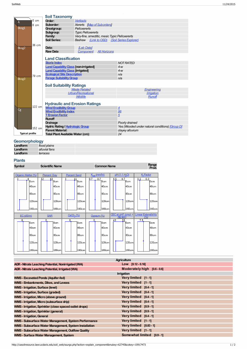
Typical profile

Soil TaxonomyOrder: VertisolsSuborder: Xererts [Map of Suborders]Greatgroup: PelloxerertsSubgroup: Typic PelloxerertsFamily: Very-fine, smectitic, mesic Typic PelloxerertsSoil Series: Bashaw (Link to OSD) (Soil Series Explorer) Data: [Lab Data]Raw Data Component All Horizons

Land ClassificationStorie Index NOT RATEDLand Capability Class [non-irrigated] 4-wLand Capability Class [irrigated] 4-wEcological Site Description n/aForage Suitability Group n/a

Soil Suitability RatingsWaste Related Engineering

Urban/Recreational IrrigationWildlife Runoff

Hydraulic and Erosion RatingsWind Erodibility Group 4Wind Erodibility Index 86T Erosion Factor 5RunoffDrainage Poorly drainedHydric Rating / Hydrologic Group Yes (Wooded under natural conditions) [Group D]Parent Material: clayey alluviumTotal Plant Available Water (cm): 24

GeomorphologyLandform flood plainsLandform alluvial fansLandform terraces

PlantsSymbol Scientific Name Common Name Range

Prod.

Organic Matter (%) Percent Clay Percent Sand Ksat (mm/hr) pH (1:1 H2O) Kf Factor

EC (dS/m) SAR CaC03 (%) Gypsum (%) CEC at pH7 (cmol +/kg soil)

Linear Extensibility(%)

AgricultureAGR - Nitrate Leaching Potential, Nonirrigated (WA) Low [0.12 - 0.16]AGR - Nitrate Leaching Potential, Irrigated (WA) Moderately high [0.6 - 0.6]

IrrigationWMS - Excavated Ponds (Aquifer-fed) Very limited [1 - 1]WMS - Embankments, Dikes, and Levees Very limited [1 - 1]WMS - Irrigation, Surface (level) Very limited [0.4 - 1]WMS - Irrigation, Surface (graded) Very limited [0.4 - 1]WMS - Irrigation, Micro (above ground) Very limited [0.4 - 1]WMS - Irrigation, Micro (subsurface drip) Very limited [0.4 - 1]WMS - Irrigation, Sprinkler (close spaced outlet drops) Very limited [0.9 - 1]WMS - Irrigation, Sprinkler (general) Very limited [0.9 - 1]WMS - Irrigation, General Very limited [0.4 - 1]WMS - Subsurface Water Management, System Performance Very limited [1 - 1]WMS - Subsurface Water Management, System Installation Very limited [0.83 - 1]WMS - Subsurface Water Management, Outflow Quality Very limited [1 - 1]WMS - Surface Water Management, System Somewhat limited [0.9 - 1]

SoilWeb 11/24/2015

http://casoilresource.lawr.ucdavis.edu/soil_web/ssurgo.php?action=explain_component&mukey=62745&cokey=10917473 1 / 2

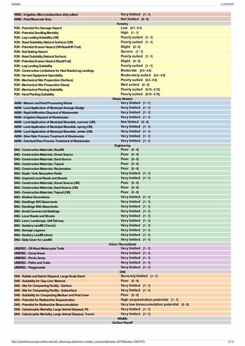
WMS - Irrigation, Micro (subsurface drip) edited Very limited [1 - 1]WMS - Pond Reservoir Area Not limited [0 - 0]

ForestryFOR - Potential Fire Damage Hazard Low [0.1 - 0.1]FOR - Potential Seedling Mortality High [1 - 1]FOR - Log Landing Suitability (OR) Poorly suited [1 - 1]FOR - Road Suitability (Natural Surface) (OR) Poorly suited [1 - 1]FOR - Potential Erosion Hazard (Off-Road/Off-Trail) Slight [0 - 0]FOR - Soil Rutting Hazard Severe [1 - 1]FOR - Road Suitability (Natural Surface) Poorly suited [1 - 1]FOR - Potential Erosion Hazard (Road/Trail) Slight [0 - 0]FOR - Log Landing Suitability Poorly suited [1 - 1]FOR - Construction Limitations for Haul Roads/Log Landings Moderate [0.5 - 0.5]FOR - Harvest Equipment Operability Moderately suited [0.5 - 0.5]FOR - Mechanical Site Preparation (Surface) Poorly suited [0.5 - 0.5]FOR - Mechanical Site Preparation (Deep) Well suited [0 - 0]FOR - Mechanical Planting Suitability Poorly suited [0.75 - 0.75]FOR - Hand Planting Suitability Poorly suited [0.75 - 0.75]

Waste RelatedAWM - Manure and Food Processing Waste Very limited [1 - 1]AWM - Land Application of Municipal Sewage Sludge Very limited [1 - 1]AWM - Rapid Infiltration Disposal of Wastewater Very limited [1 - 1]AWM - Irrigation Disposal of Wastewater Very limited [1 - 1]AWM - Land Application of Municipal Biosolids, summer (OR) Not limited [0 - 0]AWM - Land Application of Municipal Biosolids, spring (OR) Very limited [1 - 1]AWM - Land Application of Municipal Biosolids, winter (OR) Very limited [1 - 1]AWM - Slow Rate Process Treatment of Wastewater Very limited [1 - 1]AWM - Overland Flow Process Treatment of Wastewater Very limited [1 - 1]

EngineeringENG - Construction Materials; Roadfill Poor [0 - 0]ENG - Construction Materials; Gravel Source Poor [0 - 0]ENG - Construction Materials; Sand Source Poor [0 - 0]ENG - Construction Materials; Topsoil Poor [0 - 0]ENG - Construction Materials; Reclamation Poor [0 - 0]ENG - Septic Tank Absorption Fields Very limited [1 - 1]ENG - Unpaved Local Roads and Streets Very limited [1 - 1]ENG - Construction Materials; Gravel Source (OR) Poor [0 - 0]ENG - Construction Materials; Sand Source (OR) Poor [0 - 0]ENG - Construction Materials; Topsoil (OR) Poor [0 - 0]ENG - Shallow Excavations Very limited [1 - 1]ENG - Dwellings W/O Basements Very limited [1 - 1]ENG - Dwellings With Basements Very limited [1 - 1]ENG - Small Commercial Buildings Very limited [1 - 1]ENG - Local Roads and Streets Very limited [1 - 1]ENG - Lawn, Landscape, Golf Fairway Very limited [1 - 1]ENG - Sanitary Landfill (Trench) Very limited [1 - 1]ENG - Sewage Lagoons Very limited [1 - 1]ENG - Sanitary Landfill (Area) Very limited [1 - 1]ENG - Daily Cover for Landfill Very limited [1 - 1]

Urban / RecreationalURB/REC - Off-Road Motorcycle Trails Very limited [1 - 1]URB/REC - Camp Areas Very limited [1 - 1]URB/REC - Picnic Areas Very limited [1 - 1]URB/REC - Paths and Trails Very limited [1 - 1]URB/REC - Playgrounds Very limited [1 - 1]

DHSDHS - Rubble and Debris Disposal, Large-Scale Event Severely limited [1 - 1]DHS - Suitability for Clay Liner Material Poor [0 - 0]DHS - Site for Composting Facility - Surface Very limited [1 - 1]DHS - Site for Composting Facility - Subsurface Very limited [1 - 1]DHS - Suitability for Composting Medium and Final Cover Poor [0 - 0]DHS - Potential for Radioactive Sequestration High sequestration potential [1 - 1]DHS - Potential for Radioactive Bioaccumulation Very low bioaccumulation potential [0 - 0]DHS - Catastrophic Mortality, Large Animal Disposal, Pit Very limited [1 - 1]DHS - Catastrophic Mortality, Large Animal Disposal, Trench Very limited [1 - 1]

WildlifeSurface Runoff

SoilWeb 11/24/2015

http://casoilresource.lawr.ucdavis.edu/soil_web/ssurgo.php?action=explain_component&mukey=62745&cokey=10917473 2 / 2

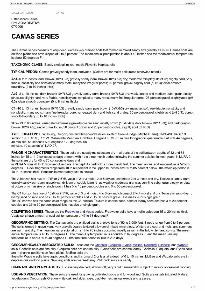
LOCATION CAMAS OR+WA

Established SeriesRev. AON/ DRJ/RWL07/2006

CAMAS SERIES

The Camas series consists of very deep, excessively drained soils that formed in mixed sandy and gravelly alluvium. Camas soils areon flood plains and have slopes of 0 to 5 percent. The mean annual precipitation is about 40 inches and the mean annual temperatureis about 52 degrees F.

TAXONOMIC CLASS: Sandy-skeletal, mixed, mesic Fluventic Haploxerolls

TYPICAL PEDON: Camas gravelly sandy loam, cultivated. (Colors are for moist soil unless otherwise noted.)

Ap1--0 to 2 inches; dark brown (10YR 3/3) gravelly sandy loam, brown (10YR 5/3) dry; moderate thin platy structure; slightly hard, veryfriable, nonsticky and nonplastic; many roots; many fine irregular pores; 20 percent gravel; slightly acid (pH 6.3); clear smoothboundary. (2 to 10 inches thick)

Ap2--2 to 10 inches; dark brown (10YR 3/3) gravelly sandy loam, brown (10YR 5/3) dry; weak coarse and medium subangular blockystructure; slightly hard, very friable, nonsticky and nonplastic; many roots; many fine irregular pores; 25 percent gravel; slightly acid (pH6.3); clear smooth boundary. (0 to 8 inches thick)

C1--10 to 13 inches; brown (10YR 4/3) gravelly sandy loam, pale brown (10YR 6/3) dry; massive; soft, very friable, nonsticky andnonplastic; many roots; many fine irregular pore; variegated dark and light sand grains; 30 percent gravel; slightly acid (pH 6.3); abruptsmooth boundary. (0 to 10 inches thick)

2C2--13 to 60 inches; variegated extremely gravelly coarse sand mostly brown (10YR 4/3); dark brown (10YR 3/3); and dark grayishbrown (10YR 4/2); single grain; loose; 50 percent gravel and 20 percent cobbles; slightly acid (pH 6.3).

TYPE LOCATION: Linn County, Oregon; one and three-fourths miles south of Green Bridge (Mitchell Farm); NW1/4SE1/4SE1/4section 19, T. 10 S., R. 2 W.; Willamette Meridian, Crabtree, Oregon USGS 7.5 minute topographic quadrangle. Latitude 44 degrees,40 minutes, 51 seconds N.; Longitude 122 degrees, 58minutes, 19 seconds W. NAD 27.

RANGE IN CHARACTERISTICS: These soils are usually moist but are dry in all parts of the soil between depths of 12 and 35inches for 45 to 110 consecutive days or more within the three month period following the summer solstice in most years. In MLRA 2,the soils are dry for 45 to 70 consecutive days andin MLRA 5 from 70 to 110 consecutive days. The depth to bedrock is more than 6 feet. The mean annual soil temperature is 52 to 55degrees F. Rock fragments range from 10 to 60 percent in the upper 15 inches and 35 to 85 percent below. The mollic epipedon is10 to 14 inches thick. Reaction is moderately acid to neutral.

The A horizon has hue of 10YR or 7.5YR, value of 2 or 3 moist, 2 to 5 dry and chroma of 2 or 3 moist and dry. Texture is sandy loam,gravelly sandy loam, very gravelly sandy loam or cobbly loam. It has weak or moderate granular, very fine subangular blocky, or platystructure or is massive or single grain. It has 0 to 10 percent cobbles and 0 to 50 percent gravel.

The C1 horizon has hue of 10YR or 7.5YR, value of 3 or 4 moist, 4 to 6 dry and chroma of 2 to 4 moist and dry. Texture is sandy loam,loamy sand or sand and has 0 to 10 percent cobbles and 20 to 50 percent gravel. It is massive or single grain. The 2C horizon has the same color range as the C1 horizon. Texture is coarse sand, sand or loamy sand and has 3 to 20 percentcobbles and 35 to 70 percent gravel. It is massive or single grain.

COMPETING SERIES: These are the Freewater and Voats series. Freewater soils have a mollic epipedon 15 to 20 inches thick.Voats soils have a mean annual soil temperature of 47 to 53 degrees F.

GEOGRAPHIC SETTING: The Camas soils are on flood plains at elevations of 50 to 3,000 feet. Slopes range from 0 to 5 percent.The soils formed in gravelly and very gravelly coarse textured alluvium of mixed mineralogy. Winters are cool and moist and summersare warm and dry. The mean annual precipitation is 18 to 70 inches occurring mostly as rain in the fall, winter, and spring. The meanannual temperature is 48 to 55 degrees F. The mean July temperature is about 65 to 67 degrees F. and the mean Januarytemperature is about 39 to 40 degrees F. The frost-free period is 150 to 235 days.

GEOGRAPHICALLY ASSOCIATED SOILS: These are the Chehalis, Cloquato, Evans, McBee, Newberg, Pilchuck, and Wapatosoils. Chehalis soils are fine-silty. Cloquato soils are coarse-silty. Evans soils are coarse-loamy. Chehalis, Cloquato, and Evans soilsare in channel positions on flood plains. McBee soils arefine-silty. Wapato soils have aquic conditions and hcroma of 2 or less at a depth of 0 to 10 inches. McBee and Wapato soils are indepressions on flood plains. Newberg soils are coarse-loamy. Philchuck soils are sandy.

DRAINAGE AND PERMEABILITY: Excessively drained; slow runoff; very rapid permeability; subject to rare or occasional flooding.

USE AND VEGETATION: These soils are used for growing cultivated crops and for woodland. Soils are usually irrigated. Naturalvegetation is Oregon ash, Oregon white oak, red alder, rose, blackberries, annual weeds and grasses.

Official Series Description - CAMAS Series 11/24/2015

https://soilseries.sc.egov.usda.gov/OSD_Docs/C/CAMAS.html 1 / 2

DISTRIBUTION AND EXTENT: Flood plains in western Oregon and Washington. The series is of moderate extent.

MLRA SOIL SURVEY REGIONAL OFFICE (MO) RESPONSIBLE: Portland, Oregon

SERIES ESTABLISHED: Southwestern Washington Reconnaissance, 1911.

REMARKS: Diagnostic horizons and features included in this pedon are:

Mollic epipedon - from the surface to 10 inches (Ap1 and Ap2 horizons).Particle-size control section - from 10 to 40 inches averaging 66 percent rock fragments.

National Cooperative Soil SurveyU.S.A.

Official Series Description - CAMAS Series 11/24/2015

https://soilseries.sc.egov.usda.gov/OSD_Docs/C/CAMAS.html 2 / 2

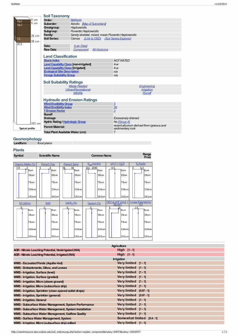
Typical profile

Soil TaxonomyOrder: MollisolsSuborder: Xerolls [Map of Suborders]Greatgroup: HaploxerollsSubgroup: Fluventic HaploxerollsFamily: Sandy-skeletal, mixed, mesic Fluventic HaploxerollsSoil Series: Camas (Link to OSD) (Soil Series Explorer) Data: [Lab Data]Raw Data Component All Horizons

Land ClassificationStorie Index NOT RATEDLand Capability Class [non-irrigated] 4-wLand Capability Class [irrigated] 4-wEcological Site Description n/aForage Suitability Group n/a

Soil Suitability RatingsWaste Related Engineering

Urban/Recreational IrrigationWildlife Runoff

Hydraulic and Erosion RatingsWind Erodibility Group 5Wind Erodibility Index 56T Erosion Factor 3RunoffDrainage Excessively drainedHydric Rating / Hydrologic Group No [Group A]Parent Material: recent alluvium derived from igneous and

sedimentary rockTotal Plant Available Water (cm): 7

GeomorphologyLandform flood plains

PlantsSymbol Scientific Name Common Name Range

Prod.

Organic Matter (%) Percent Clay Percent Sand Ksat (mm/hr) pH (1:1 H2O) Kf Factor

EC (dS/m) SAR CaC03 (%) Gypsum (%) CEC at pH7 (cmol +/kg soil)

Linear Extensibility(%)

AgricultureAGR - Nitrate Leaching Potential, Nonirrigated (WA) High [1 - 1]AGR - Nitrate Leaching Potential, Irrigated (WA) High [1 - 1]

IrrigationWMS - Excavated Ponds (Aquifer-fed) Very limited [1 - 1]WMS - Embankments, Dikes, and Levees Very limited [1 - 1]WMS - Irrigation, Surface (level) Very limited [1 - 1]WMS - Irrigation, Surface (graded) Very limited [1 - 1]WMS - Irrigation, Micro (above ground) Very limited [1 - 1]WMS - Irrigation, Micro (subsurface drip) Very limited [1 - 1]WMS - Irrigation, Sprinkler (close spaced outlet drops) Very limited [0.97 - 1]WMS - Irrigation, Sprinkler (general) Very limited [0.97 - 1]WMS - Irrigation, General Very limited [1 - 1]WMS - Subsurface Water Management, System Performance Very limited [1 - 1]WMS - Subsurface Water Management, System Installation Very limited [1 - 1]WMS - Subsurface Water Management, Outflow Quality Very limited [1 - 1]WMS - Surface Water Management, System Somewhat limited [0.4 - 1]WMS - Irrigation, Micro (subsurface drip) edited Very limited [1 - 1]

SoilWeb 11/24/2015

http://casoilresource.lawr.ucdavis.edu/soil_web/ssurgo.php?action=explain_component&mukey=64073&cokey=10918477 1 / 2

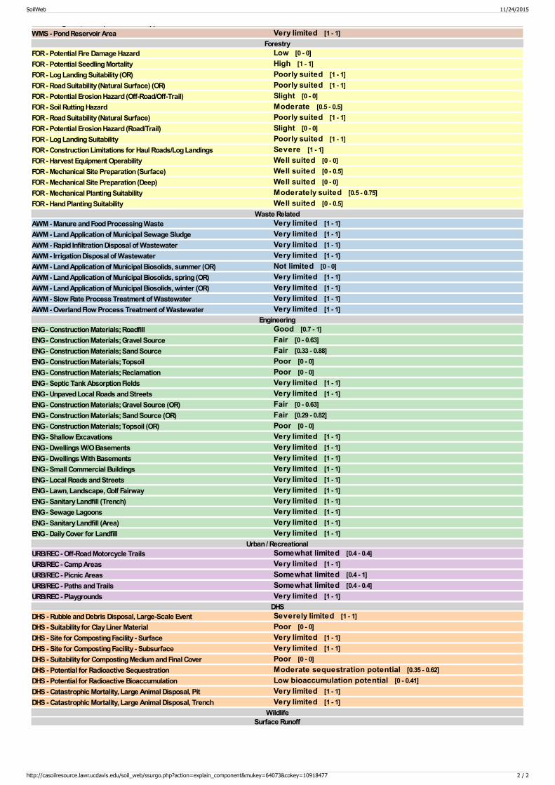
WMS - Irrigation, Micro (subsurface drip) editedWMS - Pond Reservoir Area Very limited [1 - 1]

ForestryFOR - Potential Fire Damage Hazard Low [0 - 0]FOR - Potential Seedling Mortality High [1 - 1]FOR - Log Landing Suitability (OR) Poorly suited [1 - 1]FOR - Road Suitability (Natural Surface) (OR) Poorly suited [1 - 1]FOR - Potential Erosion Hazard (Off-Road/Off-Trail) Slight [0 - 0]FOR - Soil Rutting Hazard Moderate [0.5 - 0.5]FOR - Road Suitability (Natural Surface) Poorly suited [1 - 1]FOR - Potential Erosion Hazard (Road/Trail) Slight [0 - 0]FOR - Log Landing Suitability Poorly suited [1 - 1]FOR - Construction Limitations for Haul Roads/Log Landings Severe [1 - 1]FOR - Harvest Equipment Operability Well suited [0 - 0]FOR - Mechanical Site Preparation (Surface) Well suited [0 - 0.5]FOR - Mechanical Site Preparation (Deep) Well suited [0 - 0]FOR - Mechanical Planting Suitability Moderately suited [0.5 - 0.75]FOR - Hand Planting Suitability Well suited [0 - 0.5]

Waste RelatedAWM - Manure and Food Processing Waste Very limited [1 - 1]AWM - Land Application of Municipal Sewage Sludge Very limited [1 - 1]AWM - Rapid Infiltration Disposal of Wastewater Very limited [1 - 1]AWM - Irrigation Disposal of Wastewater Very limited [1 - 1]AWM - Land Application of Municipal Biosolids, summer (OR) Not limited [0 - 0]AWM - Land Application of Municipal Biosolids, spring (OR) Very limited [1 - 1]AWM - Land Application of Municipal Biosolids, winter (OR) Very limited [1 - 1]AWM - Slow Rate Process Treatment of Wastewater Very limited [1 - 1]AWM - Overland Flow Process Treatment of Wastewater Very limited [1 - 1]

EngineeringENG - Construction Materials; Roadfill Good [0.7 - 1]ENG - Construction Materials; Gravel Source Fair [0 - 0.63]ENG - Construction Materials; Sand Source Fair [0.33 - 0.88]ENG - Construction Materials; Topsoil Poor [0 - 0]ENG - Construction Materials; Reclamation Poor [0 - 0]ENG - Septic Tank Absorption Fields Very limited [1 - 1]ENG - Unpaved Local Roads and Streets Very limited [1 - 1]ENG - Construction Materials; Gravel Source (OR) Fair [0 - 0.63]ENG - Construction Materials; Sand Source (OR) Fair [0.29 - 0.82]ENG - Construction Materials; Topsoil (OR) Poor [0 - 0]ENG - Shallow Excavations Very limited [1 - 1]ENG - Dwellings W/O Basements Very limited [1 - 1]ENG - Dwellings With Basements Very limited [1 - 1]ENG - Small Commercial Buildings Very limited [1 - 1]ENG - Local Roads and Streets Very limited [1 - 1]ENG - Lawn, Landscape, Golf Fairway Very limited [1 - 1]ENG - Sanitary Landfill (Trench) Very limited [1 - 1]ENG - Sewage Lagoons Very limited [1 - 1]ENG - Sanitary Landfill (Area) Very limited [1 - 1]ENG - Daily Cover for Landfill Very limited [1 - 1]

Urban / RecreationalURB/REC - Off-Road Motorcycle Trails Somewhat limited [0.4 - 0.4]URB/REC - Camp Areas Very limited [1 - 1]URB/REC - Picnic Areas Somewhat limited [0.4 - 1]URB/REC - Paths and Trails Somewhat limited [0.4 - 0.4]URB/REC - Playgrounds Very limited [1 - 1]

DHSDHS - Rubble and Debris Disposal, Large-Scale Event Severely limited [1 - 1]DHS - Suitability for Clay Liner Material Poor [0 - 0]DHS - Site for Composting Facility - Surface Very limited [1 - 1]DHS - Site for Composting Facility - Subsurface Very limited [1 - 1]DHS - Suitability for Composting Medium and Final Cover Poor [0 - 0]DHS - Potential for Radioactive Sequestration Moderate sequestration potential [0.35 - 0.62]DHS - Potential for Radioactive Bioaccumulation Low bioaccumulation potential [0 - 0.41]DHS - Catastrophic Mortality, Large Animal Disposal, Pit Very limited [1 - 1]DHS - Catastrophic Mortality, Large Animal Disposal, Trench Very limited [1 - 1]

WildlifeSurface Runoff

SoilWeb 11/24/2015

http://casoilresource.lawr.ucdavis.edu/soil_web/ssurgo.php?action=explain_component&mukey=64073&cokey=10918477 2 / 2

LOCATION CHITWOOD OR

Established SeriesRev. GEO/JAS/RWL11/2012

CHITWOOD SERIES

The Chitwood series consists of very deep, somewhat poorly drained soils on coastal marine and valley terraces. They formed inalluvium derived from sedimentary rocks. Slopes range from 0 to 15 percent. The mean annual temperature is about 52 degrees F.and the mean annual precipitation is about 70 inches.

TAXONOMIC CLASS: Fine, isotic, isomesic Aquandic Humudepts

TYPICAL PEDON: Chitwood medial silt loam-improved pasture, on a 2 percent slope at an elevation of 80 feet. (Colors are for moistsoil unless otherwise noted.)

Ap--0 to 7 inches; very dark grayish brown (10YR 3/2) medial silt loam, grayish brown (10YR 5/2) dry; weak very fine granularstructure; slightly hard, friable, slightly sticky and slightly plastic; weakly smeary; many very fine roots; many very fine irregular pores;strongly acid (pH 5.2); clear smooth boundary.

A--7 to 11 inches; very dark grayish brown (10YR 3/2) medial silt loam, grayish brown (10YR 5/2) dry; moderate very fine subangularblocky structure; slightly hard, friable, slightly sticky and slightly plastic; weakly smeary; many very fine roots; many very fine and fineirregular pores; very strongly acid (pH 5.0); clear smooth boundary. (Combined thickness of the A horizon is 7 to 20 inches thick)

BA--11 to 19 inches; dark brown (10YR 3/3) silty clay loam, brown (10YR 5/3) dry; moderate medium subangular blocky structureparting to moderate very fine angular blocky; moderately hard, firm, moderately sticky and moderately plastic; common fine roots;many very fine tubular pores; few fine faint continuous very dark grayish brown (10YR 3/2) organic stains on faces of peds; few finefaint dark yellowish brown (10YR 4/4) and distinct yellowish brown (10YR 5/6) iron masses, irregular in the matrix; very strongly acid(pH 5.0); clear smooth boundary. (0 to 11 inches thick)

Bw--19 to 29 inches; dark yellowish brown (10YR 3/4) silty clay, yellowish brown (10YR 5/4) dry; moderate medium subangular blockystructure parting to weak very fine angular blocky; moderately hard, firm, moderately sticky and moderately plastic; few fine roots; fewfine and common very fine tubular pores; few distinct continuous very dark grayish brown (10YR 3/2) organic stains on faces of pedsand on surfaces along pores; many medium distinct strong brown (7.5YR 5/6) iron masses, irregular in the matrix, and commonmedium distinct grayish brown (10YR 5/2) iron depletions, irregular in the matrix; very strongly acid (pH 5.0); clear smooth boundary.(10 to 40 inches thick)

BC--29 to 60 inches; dark yellowish brown (10YR 3/4) silty clay loam, yellowish brown (10YR 5/4) dry; weak subangular blockystructure; moderately hard, firm, moderately sticky and moderately plastic; few fine roots; common very fine tubular pores; commondistinct continuous very dark grayish brown (10YR 3/2) organic stains on faces of peds and on surfaces along pores; common coarseand medium prominent strong brown (7.5YR 5/8) and yellowish red (5YR 5/6) iron masses, irregular in the matrix and common coarseand medium distinct grayish brown (10YR 5/2) iron depletions, irregular in the matrix; common thin organic stains; very strongly acid(pH 4.6).

TYPE LOCATION: Tillamook County, Oregon; about 1,500 feet south and 1,000 feet east of the northwest corner of section 10,T.2S., R.9W.; USGS Tillamook topographic quadrangle; latitude 45 degrees 24 minutes 55 seconds N. and longitude 123 degrees46 minutes 31 seconds W.; NAD 27.

RANGE IN CHARACTERISTICS: The soil is usually moist, is saturated with water extended periods during the winter, and is dry forless than 45 consecutive days between the depths of about 4 to 12 inches after the summer solstice. Redox depletions with moistchroma of 2 or less are at a depth of 18 to 24 inches and represent less than 50 percent of the matrix. The mean annual soiltemperature is 50 to 54 degrees F. The difference between mean summer and mean winter soil temperature varies from 5 to 9degrees F under canopy cover. The umbric epipedon is 10 to 20 inches thick. The upper 6 to 10 inches has an estimated Alox + Feoxof 2.0 to 3.0 percent and a moist bulk density of 0.80 to 0.90 g/cc. The lower part to a depth of 20 inches, has Alox + Feox of 1.0 to 3.0percent and a moist bulk density of 0.90 to 1.0 g/cc. Andic soil properties, when present, do not extend below a depth of 14 inches. Asubstratum containing paragravel, paracobbles, and parastones is below a depth of 40 inches in some pedons.

The Ap or A horizon has hue of 10YR, value of 2 or 3 moist, 3 to 5 dry, and chroma of 2 or 3 moist and dry. Texture is dominantlymedial silt loam in the upper part and medial silt loam or silt loam in the lower part with 20 to 27 percent clay by field estimate. A fewareas are silty clay loam with 27 to 35 percent clay. It is extremely acid to moderately acid.

The BA horizon, when present, has hue of 10YR, value of 3 moist, 3 through 5 dry, and chroma of 3 moist and dry. Texture is silty clayloam with 30 to 37 percent clay. It is extremely acid to strongly acid

The Bw horizon has value of 3 through 6 moist, 4 through 7 dry and chroma of 2 through 4 moist and dry. Texture is silty clay or siltyclay loam with 35 to 45 percent clay. It is extremely acid to strongly acid.

Official Series Description - CHITWOOD Series 11/24/2015

https://soilseries.sc.egov.usda.gov/OSD_Docs/C/CHITWOOD.html 1 / 2

The BC or C horizon, when present, has hue of 10YR or 2.5Y, value of 3 through 6 moist, 4 through 7 dry, and chroma of 1 through 4moist and 2 through 4 dry. Texture is silty clay loam or silty clay with 35 to 45 percent clay and 0 to 10 percent paragravel.

COMPETING SERIES: This is the Wishkah series. Wishkah soils have an ochric epipedon and texture control section averaging 40to 50 percent clay.

GEOGRAPHIC SETTING: The Chitwood soils are on coastal marine and valley terraces. Slopes are 0 to 15 percent. The soilsformed in mixed old fine textured alluvial deposits from sedimentary rocks. Elevations range from 20 to 400 feet. The climate ischaracterized by cool wet winters and cool moist summers with fog and low clouds. The mean annual precipitation is 60 to 100inches. The average January temperature is 43 degrees F. and the average July temperature is 61 degrees F. The mean annualtemperature is 48 to 53 degrees F. The frost-free season is 160 to 300 days. These soils are on the Whiskey Run geomorphicsurface.

GEOGRAPHICALLY ASSOCIATED SOILS: These are the Hebo and Knappa soils. Hebo soils have aquic conditions with redoxconcentrations at a depth of 10 inches or less. Knappa soils are well drained and have a texture control section that averages lessthan 35 percent clay. Hebo soils are on concave areas of terraces and Knappa soils are on nearly level to convex areas of terraces.

DRAINAGE AND PERMEABILITY: Somewhat poorly drained; slow permeability. An apparent high water table is at its uppermostlimit from November through May.

USE AND VEGETATION: The soils are used for pasture and forage crops. Native vegetation is mainly of Douglas-fir, westernhemlock, western redcedar, Sitka spruce, and red alder, rose, scattered rushes and sedges, vine maple, salmonberry, westernswordfern, red elderberry, and grasses.

DISTRIBUTION AND EXTENT: Coastal valley and marine terraces of Western Oregon; MLRA 4A. The series is moderatelyextensive.

MLRA SOIL SURVEY REGIONAL OFFICE (MO) RESPONSIBLE: Portland, Oregon

SERIES ESTABLISHED: Tillamook County, Oregon, 1961.

REMARKS: Diagnostic horizons and features in this pedon include: Umbric epipedon - from the surface to 19 inches (Ap, A and BA horizon). Cambic horizon - from 19 to 29 inches (Bw horizon) Aquic feature common redox depletions beginning at a depth of 19 inches (Bw horizons). Andic subgroup feature - from 0 to 11 inches (Ap and A horizon) qualifying for andic soil properties. Based on data from NSSLsample S02OR-007-002 and on data collected for similar soils.

A proposal was submitted to NSSC (2000) to revise the definition of medial to also include those soil properties qualifying for theAndic subgroup under criteria #1 for andic soil properties. If accepted, medial modifiers would be used for those horizons meeting theandic subgroup criteria although not meeting andic soil properties.

National Cooperative Soil Survey U.S.A.

Official Series Description - CHITWOOD Series 11/24/2015

https://soilseries.sc.egov.usda.gov/OSD_Docs/C/CHITWOOD.html 2 / 2

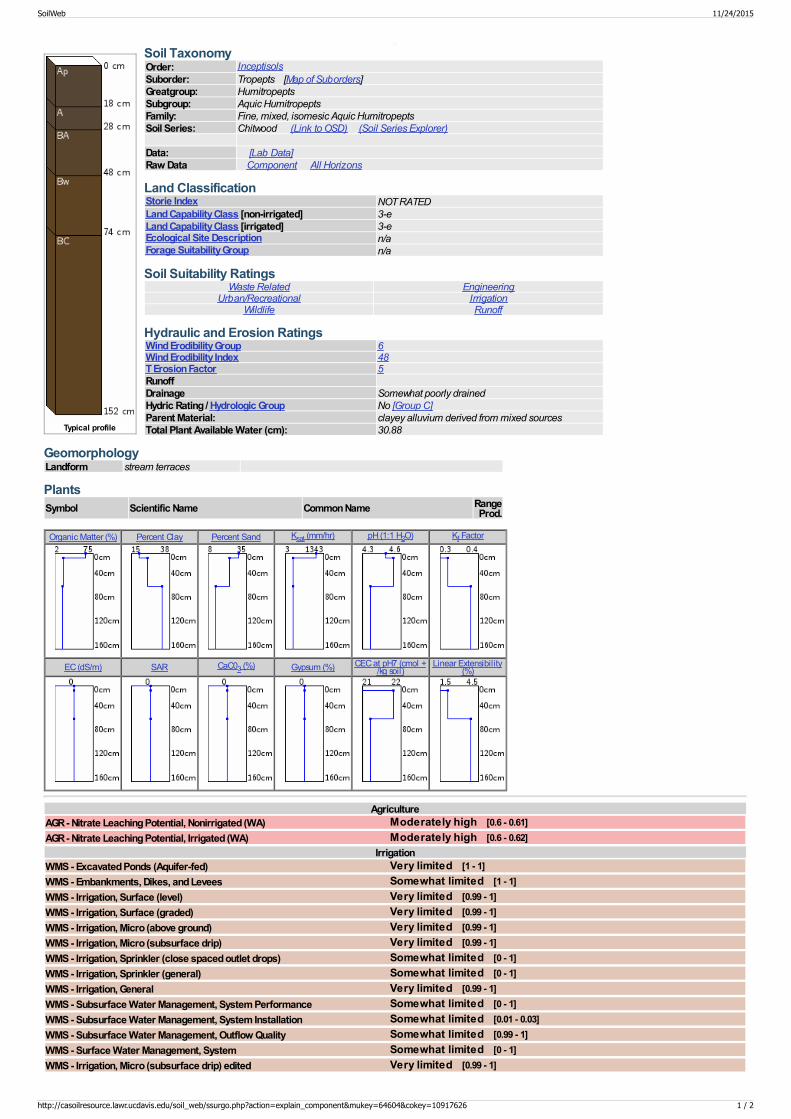
Typical profile

Soil TaxonomyOrder: InceptisolsSuborder: Tropepts [Map of Suborders]Greatgroup: HumitropeptsSubgroup: Aquic HumitropeptsFamily: Fine, mixed, isomesic Aquic HumitropeptsSoil Series: Chitwood (Link to OSD) (Soil Series Explorer) Data: [Lab Data]Raw Data Component All Horizons

Land ClassificationStorie Index NOT RATEDLand Capability Class [non-irrigated] 3-eLand Capability Class [irrigated] 3-eEcological Site Description n/aForage Suitability Group n/a

Soil Suitability RatingsWaste Related Engineering

Urban/Recreational IrrigationWildlife Runoff

Hydraulic and Erosion RatingsWind Erodibility Group 6Wind Erodibility Index 48T Erosion Factor 5RunoffDrainage Somewhat poorly drainedHydric Rating / Hydrologic Group No [Group C]Parent Material: clayey alluvium derived from mixed sourcesTotal Plant Available Water (cm): 30.88

GeomorphologyLandform stream terraces

PlantsSymbol Scientific Name Common Name Range

Prod.

Organic Matter (%) Percent Clay Percent Sand Ksat (mm/hr) pH (1:1 H2O) Kf Factor

EC (dS/m) SAR CaC03 (%) Gypsum (%) CEC at pH7 (cmol +/kg soil)

Linear Extensibility(%)

AgricultureAGR - Nitrate Leaching Potential, Nonirrigated (WA) Moderately high [0.6 - 0.61]AGR - Nitrate Leaching Potential, Irrigated (WA) Moderately high [0.6 - 0.62]

IrrigationWMS - Excavated Ponds (Aquifer-fed) Very limited [1 - 1]WMS - Embankments, Dikes, and Levees Somewhat limited [1 - 1]WMS - Irrigation, Surface (level) Very limited [0.99 - 1]WMS - Irrigation, Surface (graded) Very limited [0.99 - 1]WMS - Irrigation, Micro (above ground) Very limited [0.99 - 1]WMS - Irrigation, Micro (subsurface drip) Very limited [0.99 - 1]WMS - Irrigation, Sprinkler (close spaced outlet drops) Somewhat limited [0 - 1]WMS - Irrigation, Sprinkler (general) Somewhat limited [0 - 1]WMS - Irrigation, General Very limited [0.99 - 1]WMS - Subsurface Water Management, System Performance Somewhat limited [0 - 1]WMS - Subsurface Water Management, System Installation Somewhat limited [0.01 - 0.03]WMS - Subsurface Water Management, Outflow Quality Somewhat limited [0.99 - 1]WMS - Surface Water Management, System Somewhat limited [0 - 1]WMS - Irrigation, Micro (subsurface drip) edited Very limited [0.99 - 1]

SoilWeb 11/24/2015

http://casoilresource.lawr.ucdavis.edu/soil_web/ssurgo.php?action=explain_component&mukey=64604&cokey=10917626 1 / 2

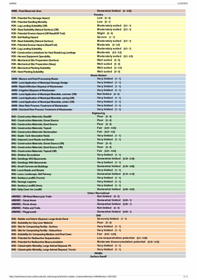
WMS - Pond Reservoir Area Somewhat limited [0 - 0.92]Forestry

FOR - Potential Fire Damage Hazard Low [0 - 0]FOR - Potential Seedling Mortality Low [0 - 1]FOR - Log Landing Suitability (OR) Moderately suited [0.5 - 1]FOR - Road Suitability (Natural Surface) (OR) Moderately suited [0.5 - 1]FOR - Potential Erosion Hazard (Off-Road/Off-Trail) Slight [0 - 0]FOR - Soil Rutting Hazard Severe [1 - 1]FOR - Road Suitability (Natural Surface) Moderately suited [0.5 - 1]FOR - Potential Erosion Hazard (Road/Trail) Moderate [0 - 0.5]FOR - Log Landing Suitability Moderately suited [0.5 - 1]FOR - Construction Limitations for Haul Roads/Log Landings Moderate [0.5 - 0.5]FOR - Harvest Equipment Operability Moderately suited [0.5 - 0.5]FOR - Mechanical Site Preparation (Surface) Well suited [0 - 0]FOR - Mechanical Site Preparation (Deep) Well suited [0 - 0]FOR - Mechanical Planting Suitability Well suited [0 - 0.5]FOR - Hand Planting Suitability Well suited [0 - 0]

Waste RelatedAWM - Manure and Food Processing Waste Very limited [1 - 1]AWM - Land Application of Municipal Sewage Sludge Very limited [1 - 1]AWM - Rapid Infiltration Disposal of Wastewater Very limited [1 - 1]AWM - Irrigation Disposal of Wastewater Very limited [1 - 1]AWM - Land Application of Municipal Biosolids, summer (OR) Not limited [0 - 0]AWM - Land Application of Municipal Biosolids, spring (OR) Very limited [1 - 1]AWM - Land Application of Municipal Biosolids, winter (OR) Very limited [1 - 1]AWM - Slow Rate Process Treatment of Wastewater Very limited [1 - 1]AWM - Overland Flow Process Treatment of Wastewater Very limited [1 - 1]

EngineeringENG - Construction Materials; Roadfill Poor [0 - 0]ENG - Construction Materials; Gravel Source Poor [0 - 0]ENG - Construction Materials; Sand Source Poor [0 - 0]ENG - Construction Materials; Topsoil Fair [0.01 - 0.53]ENG - Construction Materials; Reclamation Fair [0.27 - 0.5]ENG - Septic Tank Absorption Fields Very limited [1 - 1]ENG - Unpaved Local Roads and Streets Very limited [1 - 1]ENG - Construction Materials; Gravel Source (OR) Poor [0 - 0]ENG - Construction Materials; Sand Source (OR) Poor [0 - 0]ENG - Construction Materials; Topsoil (OR) Fair [0.01 - 0.53]ENG - Shallow Excavations Very limited [1 - 1]ENG - Dwellings W/O Basements Somewhat limited [0.39 - 0.39]ENG - Dwellings With Basements Very limited [1 - 1]ENG - Small Commercial Buildings Somewhat limited [0.39 - 0.88]ENG - Local Roads and Streets Very limited [1 - 1]ENG - Lawn, Landscape, Golf Fairway Somewhat limited [0.19 - 0.19]ENG - Sanitary Landfill (Trench) Very limited [1 - 1]ENG - Sewage Lagoons Very limited [1 - 1]ENG - Sanitary Landfill (Area) Very limited [1 - 1]ENG - Daily Cover for Landfill Somewhat limited [0.86 - 0.93]

Urban / RecreationalURB/REC - Off-Road Motorcycle Trails Not limited [0 - 0]URB/REC - Camp Areas Somewhat limited [0.85 - 1]URB/REC - Picnic Areas Somewhat limited [0.85 - 1]URB/REC - Paths and Trails Not limited [0 - 0]URB/REC - Playgrounds Somewhat limited [0.85 - 1]

DHSDHS - Rubble and Debris Disposal, Large-Scale Event Severely limited [1 - 1]DHS - Suitability for Clay Liner Material Poor [0 - 0]DHS - Site for Composting Facility - Surface Very limited [1 - 1]DHS - Site for Composting Facility - Subsurface Very limited [1 - 1]DHS - Suitability for Composting Medium and Final Cover Fair [0.01 - 0.53]DHS - Potential for Radioactive Sequestration Low sequestration potential [0.2 - 0.26]DHS - Potential for Radioactive Bioaccumulation Moderate bioaccumulation potential [0.32 - 0.32]DHS - Catastrophic Mortality, Large Animal Disposal, Pit Very limited [1 - 1]DHS - Catastrophic Mortality, Large Animal Disposal, Trench Very limited [1 - 1]

WildlifeSurface Runoff

SoilWeb 11/24/2015

http://casoilresource.lawr.ucdavis.edu/soil_web/ssurgo.php?action=explain_component&mukey=64604&cokey=10917626 2 / 2

LOCATION CLOQUATO WA+OR

Established SeriesRev. ARH/DRJ/RWL07/2006

CLOQUATO SERIES

The Cloquato series consists of very deep, well drained soils formed in mixed alluvium. Cloquato soils are on flood plains atelevations of 30 to 800 feet. Slopes are 0 to 5 percent. The mean annual temperature is about 52 degrees F. and the average annualprecipitation is about 50 inches.

TAXONOMIC CLASS: Coarse-silty, mixed, superactive, mesic Cumulic Ultic Haploxerolls

TYPICAL PEDON: Cloquato silt loam - cultivated. (Colors are for moist soil unless otherwise noted.)

Ap--0 to 7 inches; very dark grayish brown (10YR 3/2) silt loam, dark grayish brown (10YR 4/2) dry; moderate medium and coarsegranular structure; slightly hard, very friable, slightly sticky and slightly plastic; many fine roots; moderately acid; abrupt smoothboundary. (4 to 9 inches thick)

A1--7 to l2 inches; very dark grayish brown (10YR 3/2) silt loam, brown (10YR 4/3) dry; moderate medium and coarse granularstructure ; slightly hard, very friable, many fine roots; many fine and medium pores; slightly acid; clear smooth boundary. (4 to 12inches thick)

A2--l2 to 40 inches; dark brown (10YR 3/3) silt loam, brown (10YR 5/3) dry; weak fine subangular blocky structure; slightly hard, veryfriable; common fine roots; many fine and medium pores; neutral; abrupt smooth boundary. (0 to 32 inches thick)

2Cl-- 40 to 52 inches; dark grayish brown (10YR 4/2) stratified sandy loam to silt loam, grayish brown (10YR 5/2) dry; weak mediumsubangular blocky structure; soft, very friable; few fine roots; many fine and medium tubular pores; neutral; abrupt smooth boundary. (l0to 20 inches thick)

3C2--52 to 72 inches; light brownish gray (2.5Y 6/2) stratified sand to fine sandy loam, dark grayish brown (2.5Y 4/2) dry; single grain;loose; few fine roots; neutral.

TYPE LOCATION: Clark County, Washington; 1,500 feet west of northeast corner section. 31, T. 5 N., R. l E.

RANGE IN CHARACTERISTICS: The mean annual soil temperature ranges from 47 to 54 F. These soils are usually moist but aredry in all parts between depths of 4 and l2 inches for 45 to 60 consecutive days. The mollic epipedon ranges from 20 to more than 40inches thick. The particle-size control section isdominantly silt loam and contains 5 to 18 percent clay with less than l5 percent fine sand or coarser. The soil profile has a hue of l0YRor 2.5Y.

The A horizon has value of 2 or 3 moist and 4 or 5 dry, and chroma of 2 or 3 moist or dry. It has weak or moderate granular orsubangular blocky structure. This horizon is moderately acid or slightly acid in the upper part and grades to slightly acid or neutral inthe lower part.

A Bw horizon, when present, has value of 3 or 4 moist, 4 to 6 clay, and chroma of 2 to 4 moist and dry. It is slightly acid to neutral. It hasweak prismatic or weak to moderate subangular blocky structure.

The 2C and 3C horizons have value of 3 through 6 moist or dry, and chroma of 2 through 4 moist or dry. Texture is silt loam, loam, veryfine sandy loam, sandy loam, loamy sand or sand with 2 to 15 percent clay and is commonly stratified. The sandy loam, loamy sand orsand textures do not occur above a depths of 40 inches. It has 0 to 10 percent gravel. It has weak subangular blocky structure or ismassive or single grain. Reaction is neutral or slightly acid.

COMPETING SERIES: There are no other series in this family, however, similar soils include Chapman, Chehalis and McBee series.All of these soils have more than l8 percent clay in the particle-size control section. In addition, McBee soils are moderately welldrained. Chapman soils have more than 15 percent fine sand and coarser.

GEOGRAPHIC SETTING: These soils are on flood plains at elevations of 30 to 800 feet. Slopes are 0 to 5 percent. These soilsformed in mixed alluvium. Cloquato soils occur in a climate characterized by relatively cool dry summers and cool wet winters.Average annual precipitation is 38 to 70 inches. Average January temperature is 30 to 40 degrees F., average July temperature is 65to 67 degrees F., and mean annual temperature is 50 to 54 degrees F. The growing season (28F) ranges from 150 to 240 days.

GEOGRAPHICALLY ASSOCIATED SOILS: These are the Camas, Chapman, Chehalis, McBee, Newberg, Pilchuck, and Wapatosoils. Camas soils are sandy-skeletal. Pilchuck soils are sandy. Camas and Philchuck soils are on bar positions. Newberg soils arecoarse-loamy and have a mollic epipedon less than 20 inches thick. Wapato soils are poorly drained and are in depressions on floodplains. Chapman soils are on higher flood plains. McBee soils are in depressions on flood plains.

DRAINAGE AND PERMEABILITY: Well-drained; slow runoff; moderate permeability. These soils are subject to occasional floodingfor brief periods from November to March unless protected.

Official Series Description - CLOQUATO Series 11/24/2015

https://soilseries.sc.egov.usda.gov/OSD_Docs/C/CLOQUATO.html 1 / 2

USE AND VEGETATION: This soil is used for cropland, pasture and woodland. Hay, winter wheat, oats, corn for silage, potatoes,strawberries and raspberries are common crops. Native vegetation is Douglas-fir, red alder, western redcedar, and bigleaf maplewith an understory of western swordfern, vine maple, western brakenfern, salal, oregongrape, trailing blackberry, salmonberry and redhuckleberry.

DISTRIBUTION AND EXTENT: Western Washington and northwestern Oregon; MLRA 2. The series is of moderate extent.

MLRA SOIL SURVEY REGIONAL OFFICE (MO) RESPONSIBLE: Portland, Oregon

SERIES ESTABLISHED: Grays Harbor County, Washington, l970. REMARKS: Diagnostic horizons and features recognized in this pedon are:

Mollic epipedon - the zone from 0 to 40 inches with an assumed irregular decrease in organic carbon with depth. Ultic feature - base saturation (sum) of 75 percent or less in at least one horizon between 10 and 50 inches. Particle-size control section - the zone from 10 to 40 inches.

ADDITIONAL DATA; National Soil Survey Lab soil survey sample numbers: S62OR-071-015 and S62OR-071-016.

National Cooperative Soil SurveyU.S.A.

Official Series Description - CLOQUATO Series 11/24/2015

https://soilseries.sc.egov.usda.gov/OSD_Docs/C/CLOQUATO.html 2 / 2

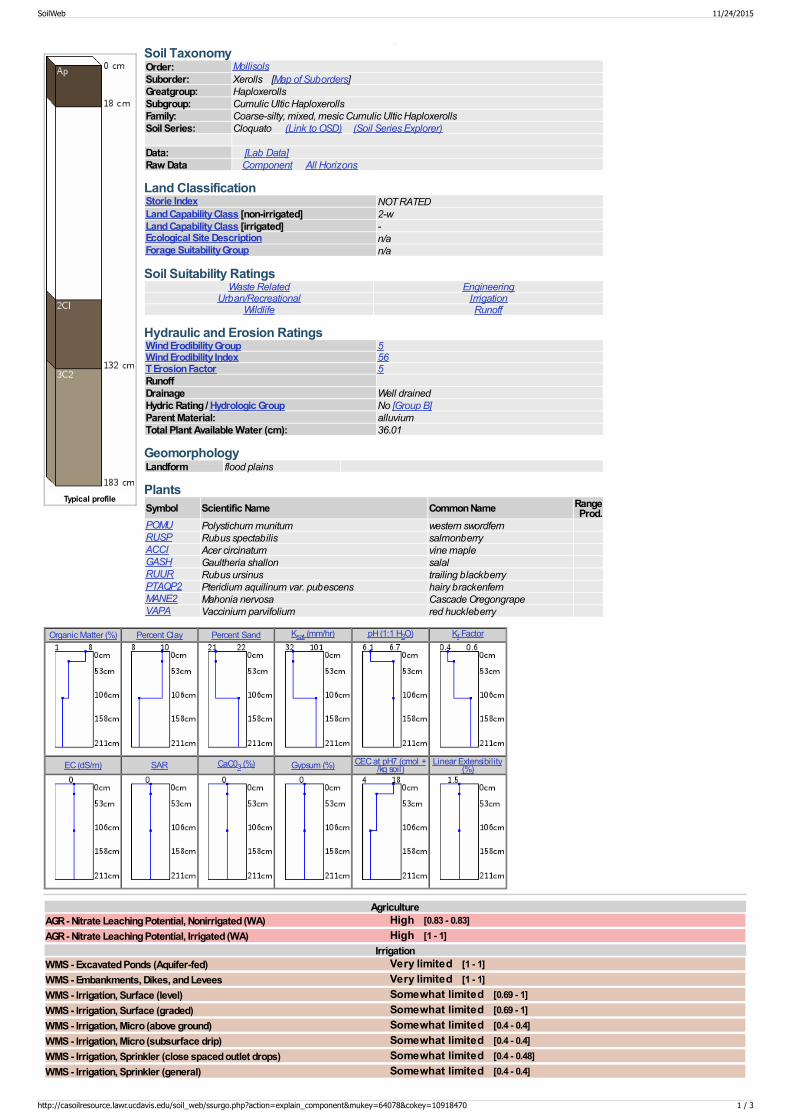
Typical profile

Soil TaxonomyOrder: MollisolsSuborder: Xerolls [Map of Suborders]Greatgroup: HaploxerollsSubgroup: Cumulic Ultic HaploxerollsFamily: Coarse-silty, mixed, mesic Cumulic Ultic HaploxerollsSoil Series: Cloquato (Link to OSD) (Soil Series Explorer) Data: [Lab Data]Raw Data Component All Horizons

Land ClassificationStorie Index NOT RATEDLand Capability Class [non-irrigated] 2-wLand Capability Class [irrigated] -Ecological Site Description n/aForage Suitability Group n/a

Soil Suitability RatingsWaste Related Engineering

Urban/Recreational IrrigationWildlife Runoff

Hydraulic and Erosion RatingsWind Erodibility Group 5Wind Erodibility Index 56T Erosion Factor 5RunoffDrainage Well drainedHydric Rating / Hydrologic Group No [Group B]Parent Material: alluviumTotal Plant Available Water (cm): 36.01

GeomorphologyLandform flood plains

PlantsSymbol Scientific Name Common Name Range

Prod.POMU Polystichum munitum western swordfernRUSP Rubus spectabilis salmonberryACCI Acer circinatum vine mapleGASH Gaultheria shallon salalRUUR Rubus ursinus trailing blackberryPTAQP2 Pteridium aquilinum var. pubescens hairy brackenfernMANE2 Mahonia nervosa Cascade OregongrapeVAPA Vaccinium parvifolium red huckleberry

Organic Matter (%) Percent Clay Percent Sand Ksat (mm/hr) pH (1:1 H2O) Kf Factor

EC (dS/m) SAR CaC03 (%) Gypsum (%) CEC at pH7 (cmol +/kg soil)

Linear Extensibility(%)

AgricultureAGR - Nitrate Leaching Potential, Nonirrigated (WA) High [0.83 - 0.83]AGR - Nitrate Leaching Potential, Irrigated (WA) High [1 - 1]

IrrigationWMS - Excavated Ponds (Aquifer-fed) Very limited [1 - 1]WMS - Embankments, Dikes, and Levees Very limited [1 - 1]WMS - Irrigation, Surface (level) Somewhat limited [0.69 - 1]WMS - Irrigation, Surface (graded) Somewhat limited [0.69 - 1]WMS - Irrigation, Micro (above ground) Somewhat limited [0.4 - 0.4]WMS - Irrigation, Micro (subsurface drip) Somewhat limited [0.4 - 0.4]WMS - Irrigation, Sprinkler (close spaced outlet drops) Somewhat limited [0.4 - 0.48]WMS - Irrigation, Sprinkler (general) Somewhat limited [0.4 - 0.4]

SoilWeb 11/24/2015

http://casoilresource.lawr.ucdavis.edu/soil_web/ssurgo.php?action=explain_component&mukey=64078&cokey=10918470 1 / 3

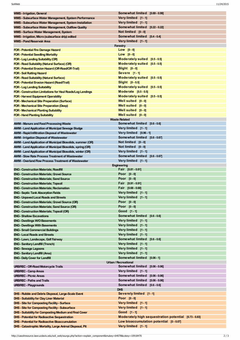
WMS - Irrigation, General Somewhat limited [0.69 - 0.99]WMS - Subsurface Water Management, System Performance Very limited [1 - 1]WMS - Subsurface Water Management, System Installation Very limited [1 - 1]WMS - Subsurface Water Management, Outflow Quality Somewhat limited [0.22 - 0.22]WMS - Surface Water Management, System Not limited [0 - 0]WMS - Irrigation, Micro (subsurface drip) edited Somewhat limited [0.4 - 0.4]WMS - Pond Reservoir Area Very limited [1 - 1]

ForestryFOR - Potential Fire Damage Hazard Low [0 - 0]FOR - Potential Seedling Mortality Low [0 - 0]FOR - Log Landing Suitability (OR) Moderately suited [0.5 - 0.5]FOR - Road Suitability (Natural Surface) (OR) Moderately suited [0.5 - 0.5]FOR - Potential Erosion Hazard (Off-Road/Off-Trail) Slight [0 - 0]FOR - Soil Rutting Hazard Severe [1 - 1]FOR - Road Suitability (Natural Surface) Moderately suited [0.5 - 0.5]FOR - Potential Erosion Hazard (Road/Trail) Slight [0 - 0.5]FOR - Log Landing Suitability Moderately suited [0.5 - 0.5]FOR - Construction Limitations for Haul Roads/Log Landings Moderate [0.5 - 0.5]FOR - Harvest Equipment Operability Moderately suited [0.5 - 0.5]FOR - Mechanical Site Preparation (Surface) Well suited [0 - 0]FOR - Mechanical Site Preparation (Deep) Well suited [0 - 0]FOR - Mechanical Planting Suitability Well suited [0 - 0]FOR - Hand Planting Suitability Well suited [0 - 0]

Waste RelatedAWM - Manure and Food Processing Waste Somewhat limited [0.6 - 0.6]AWM - Land Application of Municipal Sewage Sludge Very limited [1 - 1]AWM - Rapid Infiltration Disposal of Wastewater Very limited [0.96 - 1]AWM - Irrigation Disposal of Wastewater Somewhat limited [0.6 - 0.67]AWM - Land Application of Municipal Biosolids, summer (OR) Not limited [0 - 0]AWM - Land Application of Municipal Biosolids, spring (OR) Not limited [0 - 0]AWM - Land Application of Municipal Biosolids, winter (OR) Very limited [1 - 1]AWM - Slow Rate Process Treatment of Wastewater Somewhat limited [0.6 - 0.67]AWM - Overland Flow Process Treatment of Wastewater Very limited [1 - 1]

EngineeringENG - Construction Materials; Roadfill Fair [0.81 - 0.81]ENG - Construction Materials; Gravel Source Poor [0 - 0]ENG - Construction Materials; Sand Source Poor [0 - 0]ENG - Construction Materials; Topsoil Fair [0.91 - 0.91]ENG - Construction Materials; Reclamation Fair [0.68 - 0.68]ENG - Septic Tank Absorption Fields Very limited [1 - 1]ENG - Unpaved Local Roads and Streets Very limited [1 - 1]ENG - Construction Materials; Gravel Source (OR) Poor [0 - 0]ENG - Construction Materials; Sand Source (OR) Poor [0 - 0]ENG - Construction Materials; Topsoil (OR) Good [1 - 1]ENG - Shallow Excavations Somewhat limited [0.6 - 0.6]ENG - Dwellings W/O Basements Very limited [1 - 1]ENG - Dwellings With Basements Very limited [1 - 1]ENG - Small Commercial Buildings Very limited [1 - 1]ENG - Local Roads and Streets Very limited [1 - 1]ENG - Lawn, Landscape, Golf Fairway Somewhat limited [0.6 - 0.6]ENG - Sanitary Landfill (Trench) Very limited [1 - 1]ENG - Sewage Lagoons Very limited [1 - 1]ENG - Sanitary Landfill (Area) Very limited [1 - 1]ENG - Daily Cover for Landfill Somewhat limited [0.06 - 1]

Urban / RecreationalURB/REC - Off-Road Motorcycle Trails Somewhat limited [0.06 - 0.06]URB/REC - Camp Areas Very limited [1 - 1]URB/REC - Picnic Areas Somewhat limited [0.06 - 0.06]URB/REC - Paths and Trails Somewhat limited [0.06 - 0.06]URB/REC - Playgrounds Somewhat limited [0.6 - 0.6]

DHSDHS - Rubble and Debris Disposal, Large-Scale Event Severely limited [1 - 1]DHS - Suitability for Clay Liner Material Poor [0 - 0]DHS - Site for Composting Facility - Surface Very limited [1 - 1]DHS - Site for Composting Facility - Subsurface Very limited [1 - 1]DHS - Suitability for Composting Medium and Final Cover Good [1 - 1]DHS - Potential for Radioactive Sequestration Moderately high sequestration potential [0.73 - 0.83]DHS - Potential for Radioactive Bioaccumulation Low bioaccumulation potential [0 - 0.07]DHS - Catastrophic Mortality, Large Animal Disposal, Pit Very limited [1 - 1]

SoilWeb 11/24/2015

http://casoilresource.lawr.ucdavis.edu/soil_web/ssurgo.php?action=explain_component&mukey=64078&cokey=10918470 2 / 3

DHS - Catastrophic Mortality, Large Animal Disposal, Trench Very limited [1 - 1]Wildlife

Surface Runoff

SoilWeb 11/24/2015

http://casoilresource.lawr.ucdavis.edu/soil_web/ssurgo.php?action=explain_component&mukey=64078&cokey=10918470 3 / 3

LOCATION COQUILLE OR+CA WA

Established SeriesRev. JAS/TDT/RWL02/2011

COQUILLE SERIES

The Coquille series consists of very deep, very poorly drained soils that formed in mixed alluvium along tidal influenced flood plains.Slopes are 0 to 1 percent. The mean annual temperature is about 51 degrees F. and the mean annual precipitation is about 80inches.

TAXONOMIC CLASS: Fine-silty, mixed, superactive, nonacid, isomesic Fluvaquentic Endoaquepts

TYPICAL PEDON: Coquille silt loam, native vegetation. (Colors are for moist soil unless otherwise noted.)

A--0 to 6 inches; very dark gray (10YR 3/1) silt loam, gray (10YR 5/1) dry; weak medium subangular blocky structure; slightly hard,friable, slightly sticky and slightly plastic; many very fine and fine roots; many very fine irregular pores; moderately acid (pH 5.8); clearsmooth boundary. (4 to 7 inches thick)

Bw--6 to 16 inches; dark grayish brown (10YR 4/2) silt loam, grayish brown (10YR 5/2) dry; weak medium subangular blocky structure;slightly hard, friable, moderately sticky and slightly plastic; common very fine roots; many very fine tubular pores; many very fine distinctdark yellowish brown (10YR 4/6) redox concentrations; moderately acid (pH 6.0); clear smooth boundary. (8 to 20 inches thick)

C2--16 to 30 inches; dark grayish brown (10YR 4/2) silt loam, light brownish gray (10YR 6/2) dry; massive; slightly hard, friable, slightlysticky and slightly plastic; common very fine roots; many very fine tubular pores; many very fine and fine, prominent strong brown(7.5YR 5/6) redox concentrations; moderately acid (pH 6.0); clear smooth boundary. (8 to 30 inches thick)

2Cg--30 to 60 inches; dark gray (5Y 4/1) silt loam, light brownish gray (2.5Y 6/2) dry; massive; slightly hard, friable, slightly sticky andslightly plastic and very fluid; common very fine roots; many very fine tubular pores; slightly acid (pH 6.4).

TYPE LOCATION: Clatsop County, Oregon; about 175 feet N.E. of boat ramp slough; SE1/4SW1/4NW1/4 section 13, T. 8 N., R. 9W.

RANGE IN CHARACTERISTICS: The soil has a permanent high water table at or near the surface and fluctuates with the tidesunless diked and drained. Extreme high tides and high tides along with peak freshwater flows inundate the soil unless protected bydikes or levees. The mean annual soil temperature is 47 to 54 degrees F. The difference between mean summer and mean wintersoil temperature varies from 5 to 9 degrees F. Depth to the massive dark gray 2Cg horizon is 24 to 50 inches. The particle-sizecontrol section averages 20 to 35 percent clay and less than 15 percent coarser than very fine sand. Under natural conditions soil pHis moderately acid to neutral. When diked and drained soil pH is extremely acid to very strongly acid, but may be strongly acid tomoderately acid below 40 inches.

The A horizon has hue of 2.5Y or 10YR, value of 3 or 4 moist, 5 or 6 dry and chroma of 1 or 3. It is silt loam or silty clay loam and has20 to 30 percent clay.

The C horizon has hue of 10YR, 2.5Y or 5Y, value of 3 or 4 moist, 6 or 7 dry and chroma of 2. It is silt loam or silty clay loam and has 20to 35 percent clay. In some pedons it has thin lenses of fibrous peat less than 4 inches thick or has thin sand layers. It has common ormany distinct or prominent redox concentrations with 10YR to 5YR hue.

The 2C or 2Cg horizon has hue of 2.5Y to 5BG, value of 2.5, 3 or 4 moist, 6 or 7 dry and chroma of 1 or less moist and 2 or less dry. Itconsists of bay sediments stratified with medium to fine textured materials and thin fine lenses of peat and coarse textured materials.Some pedons have fine sand substratums below 40 inches. It is loam, silty clay loam, silty clay or clay with 25 to 65 percent clay.

COMPETING SERIES: There are no competing series.

GEOGRAPHIC SETTING: Coquille soils have formed in slightly higher areas of tide influenced flood plains along bays and streamsthat flow into the ocean. The soils formed in recent alluvium over massive bay sediments. Slopes are 0 to 1 percent. They are atelevations of 0 to 20 feet and are subject to tidal and freshwater overflow unless protected by dikes or levees. The climate ischaracterized by cool moist summers and cool wet winters. The mean annual precipitation is 60 to 120 inches. The average Julytemperature is about 59 degrees F. the average January temperature is about 38 degrees F. The mean annual air temperature is 45to 54 degrees F. The frost-free season is 180 to 245 days. The soils are on the Ingram geomorphic surface.

GEOGRAPHICALLY ASSOCIATED SOILS: These are the Brallier, Brenner, Clatsop, Nehalem and Nestucca soils. Brallier soilsare Histosols. Brenner, Nehalem and Nestucca soils have umbric epipedons and are on flood plains. Clatsop soils have a histicepipedon.

DRAINAGE AND PERMEABILITY: Very poorly drained; very slow runoff or ponded; slow permeability. Subject to tidal and

Official Series Description - COQUILLE Series 11/24/2015

https://soilseries.sc.egov.usda.gov/OSD_Docs/C/COQUILLE.html 1 / 2

freshwater overflow unless protected by dikes or levees.

USE AND VEGETATION: Native vegetation consists primarily of willow, salmonberry, tussocks, tufted hairgrass, Oregon gumweed,Douglas aster, saltgress, seaside plaintain and pickleweed.. Where protected by dikes or levees and drained, permanent pasture isthe major use. In the unprotected area, Coquille soils are important for wetland wildlife habitat.

DISTRIBUTION AND EXTENT: Tide influenced areas of western Oregon, California and Washington; MLRA 4A and 4B. The seriesis not extensive.

MLRA SOIL SURVEY REGIONAL OFFICE (MO) RESPONSIBLE: Portland, Oregon

SERIES ESTABLISHED: Marshfield Area, Oregon, 1909.

REMARKS: Diagnostic horizons and features recognized in this pedon:

Ochric epipedon - from the surface to 6 inches (A horizon)

Cambic horizon from 6 to 16 inches (Bw horizon)

Aquic moisture regime - chroma of 2 or less with redox concentrations at 6 inches.

Drained areas would be re-correlated to the Nuby Series. Nuby soils have similar landscape position and are in the acid family.

National Cooperative Soil Survey U.S.A.

Official Series Description - COQUILLE Series 11/24/2015

https://soilseries.sc.egov.usda.gov/OSD_Docs/C/COQUILLE.html 2 / 2

Typical profile

Soil TaxonomyOrder: InceptisolsSuborder: Aquepts [Map of Suborders]Greatgroup: EndoaqueptsSubgroup: Fluvaquentic EndoaqueptsFamily: Fine-silty, mixed, superactive, nonacid, isomesic Fluvaquentic EndoaqueptsSoil Series: Coquille (Link to OSD) (Soil Series Explorer) Data: [Lab Data]Raw Data Component All Horizons

Land ClassificationStorie Index NOT RATEDLand Capability Class [non-irrigated] 5-wLand Capability Class [irrigated] -Ecological Site Description n/aForage Suitability Group n/a

Soil Suitability RatingsWaste Related Engineering

Urban/Recreational IrrigationWildlife Runoff

Hydraulic and Erosion RatingsWind Erodibility Group 6Wind Erodibility Index 48T Erosion Factor 5RunoffDrainage Very poorly drainedHydric Rating / Hydrologic Group Yes (Wooded under natural conditions) [Group C/D]Parent Material: estuarine depositsTotal Plant Available Water (cm): 29.84

GeomorphologyLandscape lowlandsLandform tidal marshesLandform estuaries

PlantsSymbol Scientific Name Common Name Range

Prod.ALRU2 Alnus rubra red alderPISI Picea sitchensis Sitka spruceDECA18 Deschampsia caespitosa tufted hairgrassJUNCU Juncus rushCAREX Carex sedgeRANUN Ranunculus buttercupSALIX Salix willowFESTU Festuca fescueAREGE Argentina egedii ssp. egedii Pacific silverweed

Organic Matter (%) Percent Clay Percent Sand Ksat (mm/hr) pH (1:1 H2O) Kf Factor

EC (dS/m) SAR CaC03 (%) Gypsum (%) CEC at pH7 (cmol +/kg soil)

Linear Extensibility(%)

AgricultureAGR - Nitrate Leaching Potential, Nonirrigated (WA) Low [0.1 - 0.1]AGR - Nitrate Leaching Potential, Irrigated (WA) Moderately high [0.6 - 0.6]

IrrigationWMS - Excavated Ponds (Aquifer-fed) Somewhat limited [0.1 - 0.89]WMS - Embankments, Dikes, and Levees Very limited [1 - 1]WMS - Irrigation, Surface (level) Very limited [1 - 1]WMS - Irrigation, Surface (graded) Very limited [1 - 1]WMS - Irrigation, Micro (above ground) Very limited [1 - 1]

SoilWeb 11/24/2015

http://casoilresource.lawr.ucdavis.edu/soil_web/ssurgo.php?action=explain_component&mukey=64605&cokey=10917627 1 / 3

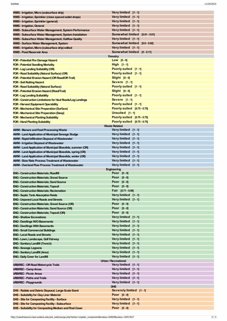
WMS - Irrigation, Micro (subsurface drip) Very limited [1 - 1]WMS - Irrigation, Sprinkler (close spaced outlet drops) Very limited [1 - 1]WMS - Irrigation, Sprinkler (general) Very limited [1 - 1]WMS - Irrigation, General Very limited [1 - 1]WMS - Subsurface Water Management, System Performance Very limited [1 - 1]WMS - Subsurface Water Management, System Installation Somewhat limited [0.01 - 0.01]WMS - Subsurface Water Management, Outflow Quality Very limited [1 - 1]WMS - Surface Water Management, System Somewhat limited [0.6 - 0.92]WMS - Irrigation, Micro (subsurface drip) edited Very limited [1 - 1]WMS - Pond Reservoir Area Somewhat limited [0 - 0.11]

ForestryFOR - Potential Fire Damage Hazard Low [0 - 0]FOR - Potential Seedling Mortality High [1 - 1]FOR - Log Landing Suitability (OR) Poorly suited [1 - 1]FOR - Road Suitability (Natural Surface) (OR) Poorly suited [1 - 1]FOR - Potential Erosion Hazard (Off-Road/Off-Trail) Slight [0 - 0]FOR - Soil Rutting Hazard Severe [1 - 1]FOR - Road Suitability (Natural Surface) Poorly suited [1 - 1]FOR - Potential Erosion Hazard (Road/Trail) Slight [0 - 0]FOR - Log Landing Suitability Poorly suited [1 - 1]FOR - Construction Limitations for Haul Roads/Log Landings Severe [1 - 1]FOR - Harvest Equipment Operability Poorly suited [1 - 1]FOR - Mechanical Site Preparation (Surface) Poorly suited [0.75 - 0.75]FOR - Mechanical Site Preparation (Deep) Unsuited [1 - 1]FOR - Mechanical Planting Suitability Poorly suited [0.75 - 0.75]FOR - Hand Planting Suitability Poorly suited [0.75 - 0.75]

Waste RelatedAWM - Manure and Food Processing Waste Very limited [1 - 1]AWM - Land Application of Municipal Sewage Sludge Very limited [1 - 1]AWM - Rapid Infiltration Disposal of Wastewater Very limited [1 - 1]AWM - Irrigation Disposal of Wastewater Very limited [1 - 1]AWM - Land Application of Municipal Biosolids, summer (OR) Very limited [1 - 1]AWM - Land Application of Municipal Biosolids, spring (OR) Very limited [1 - 1]AWM - Land Application of Municipal Biosolids, winter (OR) Very limited [1 - 1]AWM - Slow Rate Process Treatment of Wastewater Very limited [1 - 1]AWM - Overland Flow Process Treatment of Wastewater Very limited [1 - 1]

EngineeringENG - Construction Materials; Roadfill Poor [0 - 0]ENG - Construction Materials; Gravel Source Poor [0 - 0]ENG - Construction Materials; Sand Source Poor [0 - 0]ENG - Construction Materials; Topsoil Poor [0 - 0]ENG - Construction Materials; Reclamation Fair [0.71 - 0.99]ENG - Septic Tank Absorption Fields Very limited [1 - 1]ENG - Unpaved Local Roads and Streets Very limited [1 - 1]ENG - Construction Materials; Gravel Source (OR) Poor [0 - 0]ENG - Construction Materials; Sand Source (OR) Poor [0 - 0]ENG - Construction Materials; Topsoil (OR) Poor [0 - 0]ENG - Shallow Excavations Very limited [1 - 1]ENG - Dwellings W/O Basements Very limited [1 - 1]ENG - Dwellings With Basements Very limited [1 - 1]ENG - Small Commercial Buildings Very limited [1 - 1]ENG - Local Roads and Streets Very limited [1 - 1]ENG - Lawn, Landscape, Golf Fairway Very limited [1 - 1]ENG - Sanitary Landfill (Trench) Very limited [1 - 1]ENG - Sewage Lagoons Very limited [1 - 1]ENG - Sanitary Landfill (Area) Very limited [1 - 1]ENG - Daily Cover for Landfill Very limited [1 - 1]

Urban / RecreationalURB/REC - Off-Road Motorcycle Trails Very limited [1 - 1]URB/REC - Camp Areas Very limited [1 - 1]URB/REC - Picnic Areas Very limited [1 - 1]URB/REC - Paths and Trails Very limited [1 - 1]URB/REC - Playgrounds Very limited [1 - 1]

DHSDHS - Rubble and Debris Disposal, Large-Scale Event Severely limited [1 - 1]DHS - Suitability for Clay Liner Material Poor [0 - 0]DHS - Site for Composting Facility - Surface Very limited [1 - 1]DHS - Site for Composting Facility - Subsurface Very limited [1 - 1]DHS - Suitability for Composting Medium and Final Cover Poor [0 - 0]

SoilWeb 11/24/2015

http://casoilresource.lawr.ucdavis.edu/soil_web/ssurgo.php?action=explain_component&mukey=64605&cokey=10917627 2 / 3

DHS - Potential for Radioactive Sequestration High sequestration potential [1 - 0.95]DHS - Potential for Radioactive Bioaccumulation Low bioaccumulation potential [0 - 0.06]DHS - Catastrophic Mortality, Large Animal Disposal, Pit Very limited [1 - 1]DHS - Catastrophic Mortality, Large Animal Disposal, Trench Very limited [1 - 1]

WildlifeSurface Runoff

SoilWeb 11/24/2015

http://casoilresource.lawr.ucdavis.edu/soil_web/ssurgo.php?action=explain_component&mukey=64605&cokey=10917627 3 / 3

LOCATION MALABON OR

Established SeriesRev. RCH/DRJ/RWL08/2006

MALABON SERIES

The Malabon series consists of very deep, well drained soils formed in mixed alluvium. Malabon soils are on stream terraces. Slopesare 0 to 3 percent. The mean annual precipitation is about 45 inches and the mean annual temperature is about 52 degrees F.

TAXONOMIC CLASS: Fine, mixed, superactive, mesic Pachic Ultic Argixerolls

TYPICAL PEDON: Malabon silty clay loam, cultivated. (Colors are for moist soil unless otherwise noted.)

Ap--0 to 7 inches; very dark brown (10YR 2/2) silty clay loam, dark grayish brown (10YR 4/2) dry; strong very fine granular structure;hard, friable, slightly sticky and slightly plastic; many very fine roots; many irregular pores; moderately acid (pH 5.6); clear smoothboundary. (6 to 11 inches thick)

AB--7 to 12 inches; dark brown (7.5YR 3/2) silty clay loam, dark grayish brown (10YR 4/2) dry; weak fine subangular blocky and strongvery fine granular structure; hard, friable, moderately sticky and moderately plastic; many very fine roots; many very fine and few finetubular pores; very dark brown (10YR 2/2) coatings on peds; slightly acid (pH 6.1); clear wavy boundary. (0 to 15 inches thick)

Bt1--12 to 19 inches; dark brown (10YR 3/3) silty clay, dark grayish brown (10YR 4/2) dry; moderate medium subangular blocky andmoderate very fine granular structure; hard, firm, moderately sticky and moderately plastic; common very fine roots; common fine andvery fine and few medium tubular pores; many prominent very dark grayish brown (10YR 3/2) clay films on faces of peds and alongpores; slightly acid (pH 6.3); clear wavy boundary. (6 to 20 inches thick)

Bt2--19 to 29 inches; dark brown (10YR 3/3) silty clay, brown (10YR 5/3) dry; moderate medium and very fine subangular blockystructure; very hard, firm, moderately sticky and moderately plastic; common very fine roots; common very fine and few medium tubularpores; many prominent dark brown (7.5YR 3/2) clay films on faces of peds and along pores; slightly acid (pH 6.5); clear wavyboundary. (8 to 20 inches thick)

BCt--29 to 42 inches; brown (10YR 4/3) silty clay loam, brown (10YR 5/3) dry; weak coarse subangular blocky structure; very hard,firm, slightly sticky and moderately plastic; common very fine roots; common fine and medium tubular pores; common prominent darkbrown (7.5YR 3/2) clay films on faces of peds and along pores; neutral (pH 6.8); clear wavy boundary. (0 to 20 inches thick)

2C--42 to 60 inches; brown (10YR 4/3) clay loam, brown (10YR 4/3) dry; massive; hard, friable, slightly sticky and slightly plastic; fewvery fine roots; few fine tubular pores; neutral (pH 6.9).

TYPE LOCATION: Lane County, Oregon; about 1,950 feet west and 1,950 feet north of the SE corner of section 12, T. 15 S., R. 5 W.Willamette Meridian, Harrisburg, Oregon. USGS 7.5 minutes quad. Latitude 44 degrees, 16 minutes, 43 seconds N.; and Longitude123 degrees, 14 minutes, 13 seconds W. NAD 27.

RANGE IN CHARACTERISTICS: The soil is usually moist but is dry in all parts between 4 and 12 inches during the summer for 45to 60 consecutive days within MLRA 2 but ranges to 90 days in MLRA 5. The mean annual soil temperature ranges from 52 to 55degrees F. The pscs has 35 to 45 percent clay. The solum is 40 to 60 inches thick and has 0 to 5 percent gravel. Up to 15 percentgravel are in some horizons in some pedons. The mollic epipedon is 20 to 30 inches thick. Hue is 10YR or 7.5YR.

The A horizon has value of 2 or 3 moist, 4 or 5 dry and chroma of 2 or 3 moist and dry. It has 27 to 35 percent clay and 0 to 5 percentgravel. Reaction is moderately acid or slightly acid.

The AB or BA horizon, when present, has value of 2 or 3 moist, 4 or 5 dry and chroma of 2 or 3 moist and dry. Texture is silty clay loamor silty clay with 35 to 45 percent clay. Reaction is moderately or slightly acid.

The Bt horizon has value of 3 moist to 20 inches or more, and 3 or 4 below 20 inches, value of 4 or 5 dry and chroma of 2 or 3 moist, 3or 4 dry. Texture is silty clay loam or silty clay with 35 to 45 percent clay and 0 to 5 percent gravel. Reaction is moderately acid toneutral.

The BCt horizon, when present, has 30 to 45 percent clay.

The 2C horizon, where present, has value of 3 or 4 moist, 4 to 6 dry and chroma of 3 or 4 moist and dry. Texture is silty clay loam, clayloam, loam or gravelly loam and may be stratified with sandy clay loam and fine sandy loam in some pedons. It has 0 to 30 percentgravel. Reaction is slightly acid or neutral.

COMPETING SERIES: These are the Darby, Dixonville, Mart, and Silverton series. Darby soils have a mollic epipedon 30 to 50inches thick and are darker colored by 1 or 2 units of value in the upper part of the argillic horizon. Dixonville soils have a paralithiccontact at a depth of 20 to 40 inches. Silverton soils have a lithic contact at 20 to 40 inches. Mart soils have a mean annual soiltemperature of 48 to 52 degrees F.

GEOGRAPHIC SETTING: Malabon soils are dominantly on stream terraces but are also recognized on high flood plains in some

Official Series Description - MALABON Series 11/24/2015

https://soilseries.sc.egov.usda.gov/OSD_Docs/M/MALABON.html 1 / 2

areas. Elevation is 100 to 1,100 feet. Slopes are 0 to 3 percent. The soils formed in loamy and clayey alluvium from mixed materials.The summers are warm and dry and the winters are cool and moist. The mean annual precipitation is 30 to 60 inches. The meanJanuary temperature is 39 to 40 degrees F. and the mean July temperature is 65 to 67 degrees F. The mean annual temperature is50 to 55 degrees F. The frost-free season is 160 to 235 days.

GEOGRAPHICALLY ASSOCIATED SOILS: These are the Awbrig, Clackamas, Conser, Courtney, Oxley, Salem, and thecompeting Darby, Coburg, and Redbell soils. Awbrig and Conser soils are poorly drained and occur in depressions and on lowterraces. Courtney soils are poorly drained and occur in depressions. Clackamas and Oxley soils are somewhat poorly drained. Inaddition, Clackamas soils have a very gravelly or extremely gravelly C horizon. Oxley soils are loamy-skeletal. Clackamas and Oxleysoils occur on terraces. Darby soils occur on footslopes. Coburg soils occur on high flood plains and terraces. Redbell soils occur onlow terraces.

DRAINAGE AND PERMEABILITY: Well drained; slow runoff; moderately slow permeability. Areas of Malabon soils on high floodplains are subject to rare to occasional flooding for brief periods from December to March.

USE AND VEGETATION: These soils have wide use for growing orchard, berry, vegetable, small grain, hay, pasture, and grassseed crops. Natural vegetation is Douglas fir, Oregon white oak, blackberry, Pacific poison-oak, other shrubs, and grasses.

DISTRIBUTION AND EXTENT: Stream terraces of the Willamette Valley and Umpqua Valley, Oregon; MLRA 2, 5. The series is ofmoderate extent.

MLRA SOIL SURVEY REGIONAL OFFICE (MO) RESPONSIBLE: Portland, Oregon

SERIES ESTABLISHED: Benton County Area, Oregon, 1970.

REMARKS: Diagnostic horizons and features include:

Mollic epipedon - the zone from 0 to 29 inches (Ap, AB, Bt1, Bt2 horizons)Argillic horizon - the zone from 12 to 42 inches (Bt1, Bt2, and BCt horizons)Particle-size control section - the zone from 12 to 32 inches

The Malabon soils are found on the high and low Winkle geomorphic surfaces as recognized in the Willamette Valley, Oregon. Thosesoils associated with the low Winkle surface have a flooding hazard.

The Mart soils as defined in Washington are very similar. More investigation is needed to adequately separate.

ADDITIONAL DATA: Characterization data for one pedon 67Oreg. 20-15(1-6), by OSU and published in Soil Science, Volume 109,No.5, 1970.

National Cooperative Soil SurveyU.S.A.

Official Series Description - MALABON Series 11/24/2015

https://soilseries.sc.egov.usda.gov/OSD_Docs/M/MALABON.html 2 / 2

Typical profile

Soil TaxonomyOrder: MollisolsSuborder: Xerolls [Map of Suborders]Greatgroup: ArgixerollsSubgroup: Pachic Ultic ArgixerollsFamily: Fine, mixed, superactive, mesic Pachic Ultic ArgixerollsSoil Series: Malabon (Link to OSD) (Soil Series Explorer) Data: [Lab Data]Raw Data Component All Horizons

Land ClassificationStorie Index NOT RATEDLand Capability Class [non-irrigated] 1-Land Capability Class [irrigated] 1-Ecological Site Description n/aForage Suitability Group n/a

Soil Suitability RatingsWaste Related Engineering

Urban/Recreational IrrigationWildlife Runoff

Hydraulic and Erosion RatingsWind Erodibility Group 6Wind Erodibility Index 48T Erosion Factor 5RunoffDrainage Well drainedHydric Rating / Hydrologic Group No [Group C]Parent Material: clayey and loamy alluviumTotal Plant Available Water (cm): 29.31

GeomorphologyLandform terraces

PlantsSymbol Scientific Name Common Name Range

Prod.

Organic Matter (%) Percent Clay Percent Sand Ksat (mm/hr) pH (1:1 H2O) Kf Factor

EC (dS/m) SAR CaC03 (%) Gypsum (%) CEC at pH7 (cmol +/kg soil)

Linear Extensibility(%)

AgricultureAGR - Nitrate Leaching Potential, Nonirrigated (WA) Moderately high [0.7 - 0.75]AGR - Nitrate Leaching Potential, Irrigated (WA) High [0.83 - 0.99]

IrrigationWMS - Excavated Ponds (Aquifer-fed) Very limited [1 - 1]WMS - Embankments, Dikes, and Levees Somewhat limited [0.02 - 1]WMS - Irrigation, Surface (level) Somewhat limited [0.03 - 1]WMS - Irrigation, Surface (graded) Somewhat limited [0.03 - 1]WMS - Irrigation, Micro (above ground) Not limited [0 - 0]WMS - Irrigation, Micro (subsurface drip) Not limited [0 - 0.11]WMS - Irrigation, Sprinkler (close spaced outlet drops) Somewhat limited [0 - 0.48]WMS - Irrigation, Sprinkler (general) Not limited [0 - 0]WMS - Irrigation, General Somewhat limited [0.03 - 0.99]WMS - Subsurface Water Management, System Performance Very limited [1 - 1]WMS - Subsurface Water Management, System Installation Very limited [1 - 1]WMS - Subsurface Water Management, Outflow Quality Somewhat limited [0 - 0]WMS - Surface Water Management, System Not limited [0 - 0]WMS - Irrigation, Micro (subsurface drip) edited Somewhat limited [0 - 1]

SoilWeb 11/24/2015

http://casoilresource.lawr.ucdavis.edu/soil_web/ssurgo.php?action=explain_component&mukey=85305&cokey=10913046#ENG 1 / 2

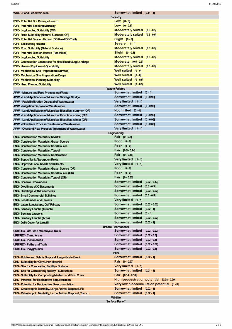
WMS - Pond Reservoir Area Somewhat limited [0.11 - 1]Forestry

FOR - Potential Fire Damage Hazard Low [0 - 0]FOR - Potential Seedling Mortality Low [0 - 0.5]FOR - Log Landing Suitability (OR) Moderately suited [0.5 - 0.5]FOR - Road Suitability (Natural Surface) (OR) Moderately suited [0.5 - 0.5]FOR - Potential Erosion Hazard (Off-Road/Off-Trail) Slight [0 - 0]FOR - Soil Rutting Hazard Severe [1 - 1]FOR - Road Suitability (Natural Surface) Moderately suited [0.5 - 0.5]FOR - Potential Erosion Hazard (Road/Trail) Slight [0 - 0.5]FOR - Log Landing Suitability Moderately suited [0.5 - 0.5]FOR - Construction Limitations for Haul Roads/Log Landings Moderate [0.5 - 0.5]FOR - Harvest Equipment Operability Moderately suited [0.5 - 0.5]FOR - Mechanical Site Preparation (Surface) Well suited [0 - 0]FOR - Mechanical Site Preparation (Deep) Well suited [0 - 0]FOR - Mechanical Planting Suitability Well suited [0 - 0.5]FOR - Hand Planting Suitability Well suited [0 - 0.5]

Waste RelatedAWM - Manure and Food Processing Waste Somewhat limited [0 - 1]AWM - Land Application of Municipal Sewage Sludge Somewhat limited [0 - 0.96]AWM - Rapid Infiltration Disposal of Wastewater Very limited [1 - 1]AWM - Irrigation Disposal of Wastewater Somewhat limited [0 - 0.96]AWM - Land Application of Municipal Biosolids, summer (OR) Not limited [0 - 0]AWM - Land Application of Municipal Biosolids, spring (OR) Somewhat limited [0 - 0.96]AWM - Land Application of Municipal Biosolids, winter (OR) Somewhat limited [0 - 0.96]AWM - Slow Rate Process Treatment of Wastewater Somewhat limited [0 - 0.85]AWM - Overland Flow Process Treatment of Wastewater Very limited [1 - 1]

EngineeringENG - Construction Materials; Roadfill Fair [0 - 0.8]ENG - Construction Materials; Gravel Source Poor [0 - 0]ENG - Construction Materials; Sand Source Poor [0 - 0]ENG - Construction Materials; Topsoil Fair [0.5 - 0.74]ENG - Construction Materials; Reclamation Fair [0 - 0.18]ENG - Septic Tank Absorption Fields Very limited [1 - 1]ENG - Unpaved Local Roads and Streets Very limited [1 - 1]ENG - Construction Materials; Gravel Source (OR) Poor [0 - 0]ENG - Construction Materials; Sand Source (OR) Poor [0 - 0]ENG - Construction Materials; Topsoil (OR) Fair [0 - 0.35]ENG - Shallow Excavations Somewhat limited [0.02 - 0.13]ENG - Dwellings W/O Basements Somewhat limited [0.5 - 0.5]ENG - Dwellings With Basements Somewhat limited [0.22 - 0.22]ENG - Small Commercial Buildings Somewhat limited [0.5 - 0.5]ENG - Local Roads and Streets Very limited [1 - 1]ENG - Lawn, Landscape, Golf Fairway Somewhat limited [0.02 - 0.02]ENG - Sanitary Landfill (Trench) Somewhat limited [0.02 - 1]ENG - Sewage Lagoons Somewhat limited [0 - 1]ENG - Sanitary Landfill (Area) Somewhat limited [0.02 - 0.02]ENG - Daily Cover for Landfill Somewhat limited [0.02 - 1]

Urban / RecreationalURB/REC - Off-Road Motorcycle Trails Somewhat limited [0.02 - 0.02]URB/REC - Camp Areas Somewhat limited [0.02 - 0.3]URB/REC - Picnic Areas Somewhat limited [0.02 - 0.3]URB/REC - Paths and Trails Somewhat limited [0.02 - 0.02]URB/REC - Playgrounds Somewhat limited [0.02 - 0.3]

DHSDHS - Rubble and Debris Disposal, Large-Scale Event Somewhat limited [0.02 - 1]DHS - Suitability for Clay Liner Material Fair [0 - 0.27]DHS - Site for Composting Facility - Surface Very limited [1 - 1]DHS - Site for Composting Facility - Subsurface Somewhat limited [0.01 - 1]DHS - Suitability for Composting Medium and Final Cover Fair [0.14 - 0.18]DHS - Potential for Radioactive Sequestration High sequestration potential [0.98 - 0.99]DHS - Potential for Radioactive Bioaccumulation Very low bioaccumulation potential [0 - 0]DHS - Catastrophic Mortality, Large Animal Disposal, Pit Somewhat limited [0.02 - 1]DHS - Catastrophic Mortality, Large Animal Disposal, Trench Somewhat limited [0.02 - 1]

WildlifeSurface Runoff

SoilWeb 11/24/2015

http://casoilresource.lawr.ucdavis.edu/soil_web/ssurgo.php?action=explain_component&mukey=85305&cokey=10913046#ENG 2 / 2

LOCATION NEHALEM OR

Established SeriesRev. JAS/AON/RWL06/2011

NEHALEM SERIES

The Nehalem series consists of very deep, well drained soils formed in mixed alluvium. Nehalem soils are on flood plains. Slopes are0 to 3 percent. The mean annual precipitation is about 90 inches and the mean annual temperature is about 50 degrees F.

TAXONOMIC CLASS: Fine-silty, mixed, superactive, isomesic Fluventic Humudepts

TYPICAL PEDON: Nehalem silt loam, on a 1 percent slope at an elevation of 15 feet in pasture. When described on August 1, 1995,the soil was moist throughout. (Colors are for moist soil unless otherwise noted.)

Ap--0 to 9 inches; very dark grayish brown (10YR 3/2) silt loam, brown (10YR 5/3) dry; moderate fine subangular blocky structure;slightly hard, friable, slightly sticky and slightly plastic; many very fine roots; many very fine tubular pores; moderately acid (pH 5.8);clear smooth boundary.

A--9 to 16 inches; dark brown (10YR 3/3) silt loam, brown (10YR 5/3) dry; moderate fine and very fine subangular blocky structure;slightly hard, friable, slightly sticky and slightly plastic; common very fine roots; many very fine tubular pores; moderately acid (pH 5.8);clear smooth boundary. (Combined thickness of the A horizon is 10 to 20 inches)

Bw--16 to 48 inches; brown (10YR 4/3) silt loam, pale brown (10YR 6/3) dry; moderate fine and medium subangular blocky structure;slightly hard, friable, slightly sticky and slightly plastic; common very fine roots; many very fine tubular pores; moderately acid (pH 6.0);gradual smooth boundary. (14 to 40 inches thick)

BC--48 to 60 inches; dark brown (10YR 3/3) silt loam, brown (10YR 5/3) dry; weak fine and medium subangular blocky structure,slightly hard, friable, slightly sticky and slightly plastic; few very fine roots; many very fine tubular pores; moderately acid (pH 6.0).

TYPE LOCATION: Tillamook County, Oregon; located about 900 feet North of the Kilchis River; about 2,200 feet north and 1,700 feetwest of the southeast corner of section 12, T. 1 S., R. 10 W.; USGS Tillamook topographic quadrangle (Latitude 45 degrees, 29minutes, 55 seconds N. and Longitude 123 degrees, 50 minutes, 55 seconds W.)

RANGE IN CHARACTERISTICS: The mean annual soil temperature is 49 to 55 degrees F. The difference between the meansummer and the mean winter soil temperature varies from 5 to 9 degrees F. The soil is usually moist and is dry in all parts betweendepths of 4 and 12 inches for a period of less than 45 consecutive days. Faint redox concentrations are below a depth of 20 inches insome pedons. The umbric epipedon is 10 to 20 inches thick. Depth to bedrock is more than 60 inches. The particle-size controlsection has 18 to 35 percent clay and less than 15 percent coarser than very fine sand. Lenses of coarser textured material are insome pedons.

The A horizon has hue of 10YR or 7.5YR, value of 2 or 3 moist, 4 or 5 dry, and chroma of 2 or 3 moist and dry. It has 15 to 25 percentclay.

The Bw horizon has hue of 10YR or 7.5YR, value of 3 or 4 moist, 5 or 6 dry, and chroma of 3 to 6 moist and dry. It is silt loam or siltyclay loam with 18 to 35 percent clay.

The BC horizon, when present, is similar to the Bw horizon. It has 18 to 35 percent clay.

The C horizon, when present, is loam, silt loam, or silty clay loam with 18 to 35 percent clay. It has 0 to 15 percent rock fragments. Insome areas, texture is very fine sandy loam or fine sandy loam below a depth of 40 inches with 12 to 20 percent clay.

COMPETING SERIES: There are no other series in this family. The Nestucca series is similar. Nestucca soils are somewhat poorlydrained and have distinct or prominent redox concentrations in the subsoil.

GEOGRAPHIC SETTING: Nehalem soils are on flood plains at elevations of 10 to 750 feet. Slopes are 0 to 3 percent. The soilsformed in medium and moderately fine textured mixed alluvial materials. The climate is humid, characterized by cool, wet winters andcool, moist summers with fog. The mean annual temperature is 48 to 53 degrees F. The mean annual precipitation is 60 to 100inches. The frost-free period is 160 to 300 days. Nehalem soils occur on the Ingram geomorphic surface.

GEOGRAPHICALLY ASSOCIATED SOILS: These are the Brenner, Coquille, Gauldy and Nestucca soils. Brenner and Coquillesoils are poorly and very poorly drained respectively. Gauldy soils are coarse-loamy over sandy or sandy-skeletal. These soils are onstream terraces.

DRAINAGE AND PERMEABILITY: Well drained; moderate permeability. Nehalem soils are subject to frequent or occasionalflooding for brief periods.

Official Series Description - NEHALEM Series 11/24/2015

https://soilseries.sc.egov.usda.gov/OSD_Docs/N/NEHALEM.html 1 / 2

USE AND VEGETATION: Nehalem soils are used for hay, pasture, and silage. Native vegetation is Douglas-fir, western hemlock,Sitka spruce, red alder, vine maple, swordfern and grasses.

DISTRIBUTION AND EXTENT: Flood plains of coastal river valleys in Western Oregon and Washington; MLRA 4A. The soil is ofmoderate extent.

MLRA SOIL SURVEY REGIONAL OFFICE (MO) RESPONSIBLE: Portland, Oregon

SERIES ESTABLISHED: Astoria Area, Clatsop County, Oregon, 1942.

REMARKS: Diagnostic horizons and features of this pedon include:

Umbric epipedon - from surface to 16 inches (Ap and A horizons).

Cambic horizon - from 16 to 60 inches.

Particle-size control section - from 10 to 40 inches.

ADDITIONAL DATA: Chemical characterization data for one pedon, S68Oreg-20-5-1 through 6, from Oregon State University.

National Cooperative Soil Survey U.S.A.

Official Series Description - NEHALEM Series 11/24/2015

https://soilseries.sc.egov.usda.gov/OSD_Docs/N/NEHALEM.html 2 / 2

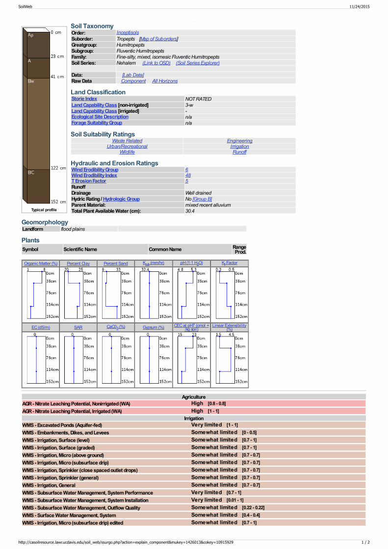
Typical profile

Soil TaxonomyOrder: InceptisolsSuborder: Tropepts [Map of Suborders]Greatgroup: HumitropeptsSubgroup: Fluventic HumitropeptsFamily: Fine-silty, mixed, isomesic Fluventic HumitropeptsSoil Series: Nehalem (Link to OSD) (Soil Series Explorer) Data: [Lab Data]Raw Data Component All Horizons

Land ClassificationStorie Index NOT RATEDLand Capability Class [non-irrigated] 3-wLand Capability Class [irrigated] -Ecological Site Description n/aForage Suitability Group n/a

Soil Suitability RatingsWaste Related Engineering

Urban/Recreational IrrigationWildlife Runoff

Hydraulic and Erosion RatingsWind Erodibility Group 6Wind Erodibility Index 48T Erosion Factor 5RunoffDrainage Well drainedHydric Rating / Hydrologic Group No [Group B]Parent Material: mixed recent alluviumTotal Plant Available Water (cm): 30.4

GeomorphologyLandform flood plains

PlantsSymbol Scientific Name Common Name Range

Prod.

Organic Matter (%) Percent Clay Percent Sand Ksat (mm/hr) pH (1:1 H2O) Kf Factor

EC (dS/m) SAR CaC03 (%) Gypsum (%) CEC at pH7 (cmol +/kg soil)

Linear Extensibility(%)

AgricultureAGR - Nitrate Leaching Potential, Nonirrigated (WA) High [0.8 - 0.8]AGR - Nitrate Leaching Potential, Irrigated (WA) High [1 - 1]

IrrigationWMS - Excavated Ponds (Aquifer-fed) Very limited [1 - 1]WMS - Embankments, Dikes, and Levees Somewhat limited [0 - 0.5]WMS - Irrigation, Surface (level) Somewhat limited [0.7 - 1]WMS - Irrigation, Surface (graded) Somewhat limited [0.7 - 1]WMS - Irrigation, Micro (above ground) Somewhat limited [0.7 - 0.7]WMS - Irrigation, Micro (subsurface drip) Somewhat limited [0.7 - 0.7]WMS - Irrigation, Sprinkler (close spaced outlet drops) Somewhat limited [0.7 - 0.7]WMS - Irrigation, Sprinkler (general) Somewhat limited [0.7 - 0.7]WMS - Irrigation, General Somewhat limited [0.7 - 0.7]WMS - Subsurface Water Management, System Performance Very limited [0.7 - 1]WMS - Subsurface Water Management, System Installation Very limited [0.01 - 1]WMS - Subsurface Water Management, Outflow Quality Somewhat limited [0.22 - 0.22]WMS - Surface Water Management, System Somewhat limited [0.4 - 0.4]WMS - Irrigation, Micro (subsurface drip) edited Somewhat limited [0.7 - 1]

SoilWeb 11/24/2015

http://casoilresource.lawr.ucdavis.edu/soil_web/ssurgo.php?action=explain_component&mukey=1426013&cokey=10915929 1 / 2

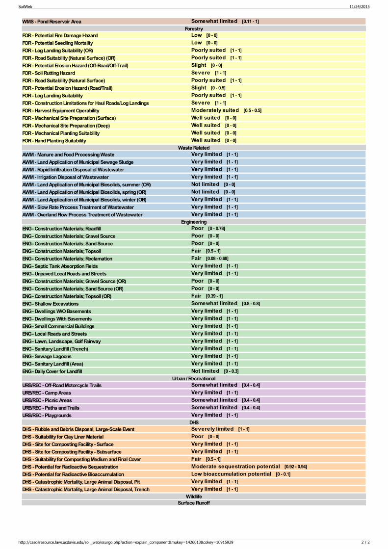
WMS - Pond Reservoir Area Somewhat limited [0.11 - 1]Forestry

FOR - Potential Fire Damage Hazard Low [0 - 0]FOR - Potential Seedling Mortality Low [0 - 0]FOR - Log Landing Suitability (OR) Poorly suited [1 - 1]FOR - Road Suitability (Natural Surface) (OR) Poorly suited [1 - 1]FOR - Potential Erosion Hazard (Off-Road/Off-Trail) Slight [0 - 0]FOR - Soil Rutting Hazard Severe [1 - 1]FOR - Road Suitability (Natural Surface) Poorly suited [1 - 1]FOR - Potential Erosion Hazard (Road/Trail) Slight [0 - 0.5]FOR - Log Landing Suitability Poorly suited [1 - 1]FOR - Construction Limitations for Haul Roads/Log Landings Severe [1 - 1]FOR - Harvest Equipment Operability Moderately suited [0.5 - 0.5]FOR - Mechanical Site Preparation (Surface) Well suited [0 - 0]FOR - Mechanical Site Preparation (Deep) Well suited [0 - 0]FOR - Mechanical Planting Suitability Well suited [0 - 0]FOR - Hand Planting Suitability Well suited [0 - 0]

Waste RelatedAWM - Manure and Food Processing Waste Very limited [1 - 1]AWM - Land Application of Municipal Sewage Sludge Very limited [1 - 1]AWM - Rapid Infiltration Disposal of Wastewater Very limited [1 - 1]AWM - Irrigation Disposal of Wastewater Very limited [1 - 1]AWM - Land Application of Municipal Biosolids, summer (OR) Not limited [0 - 0]AWM - Land Application of Municipal Biosolids, spring (OR) Not limited [0 - 0]AWM - Land Application of Municipal Biosolids, winter (OR) Very limited [1 - 1]AWM - Slow Rate Process Treatment of Wastewater Very limited [1 - 1]AWM - Overland Flow Process Treatment of Wastewater Very limited [1 - 1]

EngineeringENG - Construction Materials; Roadfill Poor [0 - 0.78]ENG - Construction Materials; Gravel Source Poor [0 - 0]ENG - Construction Materials; Sand Source Poor [0 - 0]ENG - Construction Materials; Topsoil Fair [0.5 - 1]ENG - Construction Materials; Reclamation Fair [0.08 - 0.68]ENG - Septic Tank Absorption Fields Very limited [1 - 1]ENG - Unpaved Local Roads and Streets Very limited [1 - 1]ENG - Construction Materials; Gravel Source (OR) Poor [0 - 0]ENG - Construction Materials; Sand Source (OR) Poor [0 - 0]ENG - Construction Materials; Topsoil (OR) Fair [0.39 - 1]ENG - Shallow Excavations Somewhat limited [0.8 - 0.8]ENG - Dwellings W/O Basements Very limited [1 - 1]ENG - Dwellings With Basements Very limited [1 - 1]ENG - Small Commercial Buildings Very limited [1 - 1]ENG - Local Roads and Streets Very limited [1 - 1]ENG - Lawn, Landscape, Golf Fairway Very limited [1 - 1]ENG - Sanitary Landfill (Trench) Very limited [1 - 1]ENG - Sewage Lagoons Very limited [1 - 1]ENG - Sanitary Landfill (Area) Very limited [1 - 1]ENG - Daily Cover for Landfill Not limited [0 - 0.3]

Urban / RecreationalURB/REC - Off-Road Motorcycle Trails Somewhat limited [0.4 - 0.4]URB/REC - Camp Areas Very limited [1 - 1]URB/REC - Picnic Areas Somewhat limited [0.4 - 0.4]URB/REC - Paths and Trails Somewhat limited [0.4 - 0.4]URB/REC - Playgrounds Very limited [1 - 1]

DHSDHS - Rubble and Debris Disposal, Large-Scale Event Severely limited [1 - 1]DHS - Suitability for Clay Liner Material Poor [0 - 0]DHS - Site for Composting Facility - Surface Very limited [1 - 1]DHS - Site for Composting Facility - Subsurface Very limited [1 - 1]DHS - Suitability for Composting Medium and Final Cover Fair [0.5 - 1]DHS - Potential for Radioactive Sequestration Moderate sequestration potential [0.92 - 0.94]DHS - Potential for Radioactive Bioaccumulation Low bioaccumulation potential [0 - 0.1]DHS - Catastrophic Mortality, Large Animal Disposal, Pit Very limited [1 - 1]DHS - Catastrophic Mortality, Large Animal Disposal, Trench Very limited [1 - 1]

WildlifeSurface Runoff

SoilWeb 11/24/2015

http://casoilresource.lawr.ucdavis.edu/soil_web/ssurgo.php?action=explain_component&mukey=1426013&cokey=10915929 2 / 2