Re-evaluating Surface Application Rates for Texas OSSF Systems

by

Clifford B. FedlerJohn Borrelli

Department of Civil EngineeringTexas Tech UniversityLubbock, TX 79409-1023

Texas On-Site Wastewater TreatmentResearch Council

Grant No. 582-1-83219August 31, 2001

Re-evaluating Surface Application Rates for

Texas OSSF Systems

by

Clifford B. Fedler John Borrelli

Department of Civil Engineering

Texas Tech University Lubbock, TX 79409-1023

Submitted To:

Texas Natural Resources Conservation Commission Installer Certification Section

Austin, TX 78711-3087

August 31, 2001

2

Executive Summary

Approximately 25% of the nation’s housing units utilize on-site treatment and disposal systems. Mostly, on-site treatment consists of a septic tank-soil adsorption configuration, though surface disposal systems are used in areas where the soil is not suitable for an adsorption field. One of the concerns with the use of on-site sewage treatment systems is the potential for nitrate pollution of the groundwater resources. Current procedures for designing surface application systems for on-site sewage facilities (OSSFs), with an emphasis on aerobic systems, in Texas have been reviewed. Concerns with the current procedures for designing sprinkler systems include the sizing of the spray field area, the volume of effluent storage required, and the absence of the uniformity of sprinkler distribution patterns. Currently the spray field area is determined by the estimated daily volume of water applied divided irrigation water requirement (evaporation minus precipitation). A proper design needs to be adaptable to the many climates and soils that exist within the state, while maintaining the integrity of the environment. To meet this goal, an alternative, easy to follow, design procedure is proposed. The proposed design method incorporates the concept of water application rate, soil infiltration rate, crop water use, crop nutrient uptake rate, water application efficiency, and irrigation layout design and nozzle selection.

With any surface application system for wastewater effluent, control of the nitrogen applied is essential to minimize the impact on regional water resources, whether surface water or ground water. If an OSSF is designed with a typical type of sprinkler and no overlap of the spray pattern is provided, the potential mass of nitrogen that can move below the crops root zone can be substantial. The quantity of nitrogen that could potentially move below the crops root zone ranges from 16 percent of the nitrogen applied in East Texas to 59 percent of the nitrogen applied in West Texas. Poor distribution of the effluent applied on portions of the spray field may cause the nutrients (e.g. nitrate-nitrogen) to be applied at levels exceeding the plants assimilation capacity. If a sprinkler design provides an overlapping spray pattern and the wastewater application rate is limited based on the crops ability to utilize the applied nitrogen, the nitrogen that could potentially move below the crops root zone can be limited to 7 percent of the total nitrogen applied or less. This limited nitrogen movement is realized when the wastewater distribution uniformity coefficient is 80 percent or greater.

Another advantage of the proposed design procedure is the smaller land area requirement in some parts of the state. In east Texas for example, the land area reduction is about 27 percent while the land area required in West Texas increases by two times. The additional system requirements under the proposed design procedure are an increase in the number of sprinkler heads and a zone sprinkler controller. This latter device is required to cycle the application of the wastewater effluent to the various quadrants of the spray field.

It is recommended that the following changes be made to the current Texas Administrative Code 285 rules in order to provide for the least amount of negative impact our the states environment.

3

1. All surface application systems designed for an on-site sewage facility should

consider both a water balance and a nutrient balance for the final design. 2. The layout of the site for effluent application should be in a block pattern such

that the sprinklers can be arranged to have a head-to-head overlap. If this is not available, then the system should be designed such that the proper overlap can be provided in order to achieve a uniformity coefficient of 80 percent or greater.

3. Spray head type of sprinklers should not be used in an OSSF system while the gear head type should be used.

4. All sprinklers are designed to operate at an optimum pressure range to obtain the specified pattern of water distribution and the OSSF design pressure should be in the middle of the specified range. Sprinklers operating at pressures lower or higher than designed will produce unreliable patterns that will result in very low water application efficiencies and low application uniformity.

5. The time used to apply the effluent should not exceed 1 hour and the average design should be 0.5 hours.

6. The base water intake rate of the soil should follow that described by Saxton et al. (1986) provided more precise information on the soil is not available.

7. The base soil infiltration rate should be set equal to the saturated hydraulic conductivity of the top 18 inches of soil.

8. A check-off list of design considerations should be developed and used on all new and renovated designs of OSSF where surface application of the effluent is utilized.

4

Table of Contents

Page

Executive Summary ....................................................................................... 2 Table of Contents........................................................................................... 4 List of Figures ................................................................................................ 5 List of Tables ................................................................................................. 5 List of Symbols .............................................................................................. 6 Introduction.................................................................................................... 9 Current Procedures for Designing Sprinkler Systems for OSSF Systems..... 9 Design Recommendations for OSSF Sprinkler Systems ............................... 10 Sprinkler Spacing...................................................................................... 12 Operating Pressure of System................................................................... 14 Selection of Sprinkler Heads .................................................................... 15 Pressure Losses in Main Pipeline ............................................................. 16 Risers......................................................................................................... 16 Application Rate ....................................................................................... 16 Estimating Base Intake Rate of Soil .................................................... 17 Interception .......................................................................................... 19 Time of Application............................................................................. 20 Nitrogen Control in Surface Application Systems......................................... 21 Sizing the Spray Field............................................................................... 22 Proposed Procedure to Size Spray Field.............................................. 24 Determining Nitrogen Distribution in Irrigated Area ............................... 26 Christiansen’s Uniformity Coefficient................................................. 26 Linear Distribution of Water................................................................ 27 Example for Using the Coefficient of Uniformity............................... 29 Calculations: Proposed Method ..................................................... 29 Calculations: Current TAC 285 Method........................................ 31 Recommendations.......................................................................................... 33 List of Design Considerations........................................................................ 34 References...................................................................................................... 35 Glossary ......................................................................................................... 38 Appendix-Example OSSF Designs................................................................ 40 375 gal/day......................................................................................... 41 1200 gal/day....................................................................................... 54 5000 gal/day....................................................................................... 68

5

List of Figures

page

Figure 1—Maximum Application Rates for Surface Application of Treated Effluent in Texas.............................................................................. 10 Figure 2—Shape of Sprinkler Pattern............................................................ 11 Figure 3—Overlapped Sprinkler Pattern ....................................................... 12 Figure 4—Graphic Definition of Sprinkler Spacing...................................... 13 Figure 5—Example Infiltration Curve........................................................... 17 Figure 6—Soil Textural Triangle................................................................... 19 Figure 7—Coefficient of Uniformity for Various Sprinkler Discharge Profiles ............................................................................................ 27 Figure 8—Linear Distribution of Water on Field .......................................... 29

List of Tables

page

Table 1—Generalized Soil-Water Characteristics from Texture................... 18 Table 2—Nitrogen Uptake Rates for Selected Forests .................................. 22 Table 3—Nitrogen Uptake Rates for Selected Forages................................. 23 Table 4—Nitrogen Uptake Rates for Selected Crops .................................... 23 Table 5—Water Quality of Effluent from Septic Tank ................................. 24 Table 6—Water Quality of Effluent from Aeration Tank ............................. 24 Table 7—Nitrogen Distribution by a Single Sprinkler Head......................... 31

6

List of Symbols Area The design area for the spray field, ft2 Arean The minimum area of the spray field assuming nitrogen is the land-limiting

factor, ft2 Areahyd The minimum area of the spray field assuming the intake rate of the soil or the hydraulic loading rate is the land-limiting factor, ft2 C Hazen-Williams pipe roughness factor Cn The estimated concentration of total nitrogen in the wastewater effluent, mg/l Dw The wetted diameter for a sprinkler head for a given orifice and operating

pressure, ft Ea The ratio of the average depth of irrigation water infiltrated and stored in the root zone to the average depth of irrigation water applied, percentage IB The base water intake rate (minimum) for the soil, inches/hr K The saturated hydraulic conductivity of the soil, inches/hr L Distance from the pump to the spray field or the connection to main line, ft MAR Maximum application rate for surface irrigation of treated effluent in Texas, gal/ft2/day n The number of sample points for determining the uniformity coefficient Napplied The nitrogen applied to the spray field or portion of spray field, lb/yr Nleached Amount of nitrogen leaching below root zone of spray field or portion of spray field, lb/yr Nused Amount of nitrogen used by crop in spray field or portion of spray field, lb/yr Ny The estimated yearly uptake of nitrogen by the vegetation proposed for the spray field, lb/acre/yr Nosb The number of spray blocks needed for spray field system Pa Average pressure in the lateral, psi Pd Desired operating pressure of sprinklers, psi

7

Pf Friction loss in the lateral, psi Pn

Pressure at sprinkler head nearest the pump, psi Po Pressure at sprinkler head at distal end of lateral, psi Q The estimated daily volume of water to be applied, gal/day Qendlat The total flow into the end laterals of the proposed sprinkler system, gpm Qmidlat The total flow into the middle lateral(s) of the proposed sprinkler system, gpm QR The maximum application rate adjusted for surface storage and time of application, inches/hr Qset Average flow rate for all sets, gpm Qspr Discharge rate from full-circle sprinkler head, gpm sl The sprinkler spacing along the lateral, ft sm The lateral spacing along the main, ft SL Elevation difference between the pump and the spray field, ft SS Maximum surface storage for sprinkler system, inches TA Time of application of effluent on to the spray field, hr Td Time required to drain the storage tank given the average flow rate for all sets, min Tn The estimated pounds of total nitrogen being applied as a constituent

of the wastewater effluent, lb/yr Tset The normal time of application for the proposed sprinkler system, min UCC Christiansen’s Uniformity Coefficient, percent Vol Volume of storage tank between the alarm-on level and the pump-on level, gal X X is the fraction of area having a dimensionless depth of Y or less Xi The ith single observation of depth of application by a sprinkler system, inches or volume per unit area

8

X The mean observation of depth of application by a sprinkler system, inches or volume per unit area

Y The dimensionless depth or actual depth divided by the average depth applied (field average) to the spray field Ymax The maximum actual depth applied divided by the average depth applied (field average) to the spray field Ymin The minimum actual depth applied divided by average depth applied (field average) to the spray field Θ The soil moisture content, ft3/ft3

9

Re-evaluating Surface Application Rates for Texas OSSF Systems

Introduction

Approximately 25% of the nation’s housing units utilize on-site treatment and disposal systems. With the increasing population and a trend toward moving away from urban life, the number of on-site systems in use is increasing. Even though the majority of the on-site systems consist of a septic tank-soil adsorption configuration, surface disposal systems are widely used in areas where the soil is not suitable for an adsorption field.

The rural living style of many people in Texas necessitates the use of on-site sewage treatment systems. One of the concerns with the use of these systems is the potential for nitrate pollution of groundwater resources. The design of on-site surface irrigation systems for the treatment and disposal of effluent from aerobic on-site treatment systems was addressed in this report. In order to address the design of the surface application system for effluent from an aerobic system, an assumption that no denitrification has occurred was made, therefore the primary form of nitrogen in the effluent is nitrate. A proposed method for designing sprinkler systems for on-site surface irrigation systems is the focus of this report with an emphasis on minimizing nitrogen movement below the root zone of the crop. Current Procedures for Designing Sprinkler Systems The Texas Natural Resources Conservation Commission (TNRCC) has established standards for the design of surface application systems as presented in Texas Administrative Code (TAC) Chapter 285. The surface application systems refer to sprinkler irrigation systems used for the application of effluent from on-site treatment systems. Chapter 285 specifies the method for sizing the spray field and determining the volume of effluent storage. While there are numerous details specified, the concern addressed in this report was the sizing of the spray field area and the volume of effluent storage required for the most efficient design. The spray field area is determined by taking the estimated daily volume of water to be applied and dividing it by the maximum surface application rate (MAR). The MAR is shown in Figure 1. Figure 1 was developed by determining the irrigation requirement (evapotranspiration – precipitation) across the State of Texas. This accounts for the MAR being relatively small in the eastern part of the state (an area of high precipitation) and large in the western part of the state (an area of low precipitation). No other consideration is specified such as type of crop, water intake rate of the different soil types, etc. For systems controlled by commercial irrigation timers and required to irrigate between midnight and 5:00 a.m., the required storage volume is at least one day of estimated daily volume of effluent between the alarm-on level and the pump-on level and

10

a storage volume of one-third the daily flow between the alarm-on level and the inlet to the pump tank. There appears to be no consideration given to sizing storage tanks to take into consideration the variation of effluent from day to day throughout the year. The sprinkler layout may be any design from that designed with sprinkler overlap and subsequent high coefficients of uniformity to sprinklers with no overlap. Since there are no specifications of the uniformity of sprinkler distribution pattern, the least expensive design, one without any overlap of the sprinkler patterns, is often the first choice.

Figure 1.-Maximum Application Rates for Surface Application of Treated Effluent in

Texas (gallons/ft2/day) (TAC 285.90, 2001). Design Recommendations for OSSF Sprinkler Systems The design of sprinkler systems for an On-Site Sewage Facilities (OSSF) is more like those for turf grass than for agricultural crops. The principle of the design is to contain the water on a specific area with no water going outside the boundaries of the irrigated area. To accomplish this, part-circle and full-circle sprinkler heads are used

11

rather than having all full-circle sprinkler heads. Care must be given to the overlapping pattern of the water distributed by the sprinklers so that no water is distributed outside the designated area or spray field. In addition to controlling the area wetted by the sprinkler system, there is a need to distribute the effluent uniformly. It must be realized that nutrient distribution is similar in proportions to the water (effluent in this case) being distributed by the sprinklers. Thus, poor distribution of the effluent applied on portions of the spray field may cause the nutrients (e.g. nitrate-nitrogen) to be applied at levels exceeding the plants’ assimilation capacity. In actuality, the terms uniform and poor distribution are relative terms because no sprinkler system distributes water with absolute uniformity. Sprinklers typically distribute water in a cone shaped pattern (Figure 2) and uniform distribution, relatively speaking, occurs as a result of overlapping the water distribution patterns (Figure 3). Detailed design procedures for typical solid-set sprinkler systems can be found in Keller and Bliesner (1990) and Watkins (1977). These references provide information on all aspects of sprinkler system design. Listed below are some considerations that are crucial for OSSF sprinkler systems.

Figure 2. Shape of sprinkler pattern for an individual sprinkler.

0

5

10

15

20

25

30

-40 -32 -24 -16 -8 0 8 16 24 32 40Distance from Sprinkler Head, ft

Rel

ativ

e D

epth

of W

ater

12

Figure 3. Sprinkler pattern where overlap of the spray pattern is provided.

Sprinkler Spacing There are two major design considerations for selecting the spacing of sprinkler heads—the spacing must result in an acceptable uniformity of water distribution and the effluent must be contained within the spray field. The spacing that best accomplishes these two design considerations is 0.5 times the sprinkler’s wetted diameter. The wetted diameter is the spread of water by the sprinkler head. The wetted area when operating in the absence of wind is considered to be a circle. Generally it is best to select the operating pressure, orifice size, and sprinkler head that will provide the wetted diameter needed for the selected sprinkler spacing. While there are some sprinkler heads that are adjustable to control the wetted diameter, these sprinklers should be avoided. The sprinkler spacing of 0.5 times the wetted diameter will allow for a good match of quarter-, half-, three-quarter, and full-circle sprinklers within the spray field without the problem of throwing water beyond the spray field. Most importantly, this sprinkler spacing should distribute the water with a high coefficient of uniformity (85 percent or greater is preferred). The coefficient of uniformity is a measure of water application across a field or irrigation set. Christiansen’s Uniformity Coefficients is generally used for the coefficient of uniformity and is described in detail below. A uniformity of 85 percent is recommended by Keller and Bliesne (1990) for turf systems, which is greater than the 70 percent minimum required for agricultural sprinkler systems (Pair et al., 1983). The above assumption is predicated on the sprinkler head being operated within the manufacturer’s range of recommended operating pressures, the sprinkler spacing (sl), lateral spacing along the

0

5

10

15

20

25

30

35

-40 -32 -24 -16 -8 0 8 16 24 32 40Distance from Sprinkler Head, ft

Rel

ativ

e D

epth

of W

ater

13

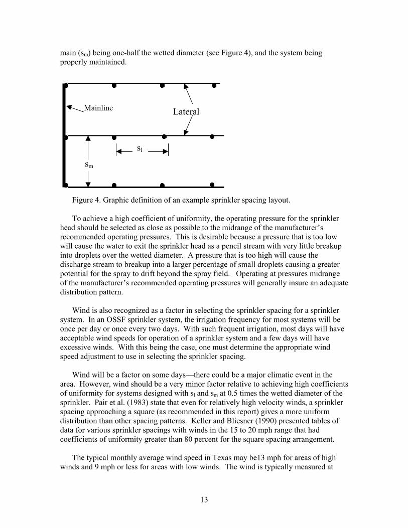
main (sm) being one-half the wetted diameter (see Figure 4), and the system being properly maintained.

Mainline Figure 4. Graphic definition of an example sprinkler spacing layout. To achieve a high coefficient of uniformity, the operating pressure for the sprinkler

head should be selected as close as possible to the midrange of the manufacturer’s recommended operating pressures. This is desirable because a pressure that is too low will cause the water to exit the sprinkler head as a pencil stream with very little breakup into droplets over the wetted diameter. A pressure that is too high will cause the discharge stream to breakup into a larger percentage of small droplets causing a greater potential for the spray to drift beyond the spray field. Operating at pressures midrange of the manufacturer’s recommended operating pressures will generally insure an adequate distribution pattern.

Wind is also recognized as a factor in selecting the sprinkler spacing for a sprinkler

system. In an OSSF sprinkler system, the irrigation frequency for most systems will be once per day or once every two days. With such frequent irrigation, most days will have acceptable wind speeds for operation of a sprinkler system and a few days will have excessive winds. With this being the case, one must determine the appropriate wind speed adjustment to use in selecting the sprinkler spacing.

Wind will be a factor on some days—there could be a major climatic event in the

area. However, wind should be a very minor factor relative to achieving high coefficients of uniformity for systems designed with sl and sm at 0.5 times the wetted diameter of the sprinkler. Pair et al. (1983) state that even for relatively high velocity winds, a sprinkler spacing approaching a square (as recommended in this report) gives a more uniform distribution than other spacing patterns. Keller and Bliesner (1990) presented tables of data for various sprinkler spacings with winds in the 15 to 20 mph range that had coefficients of uniformity greater than 80 percent for the square spacing arrangement.

The typical monthly average wind speed in Texas may be13 mph for areas of high

winds and 9 mph or less for areas with low winds. The wind is typically measured at

sm

Lateral

sl

14

11.5 to 13 ft in height above the ground surface. The wind speed at the height of the typical sprinkler (less than 3.28 ft) will be approximately 0.75 times that reported in climatological data. Jensen et al. (1990) reported that the ratio of day-time wind speeds to night-time wind speeds was 2.0, more or less. Thus, night-time wind speeds are 0.67 times the average wind speeds. Therefore, if the sprinkler irrigation occurs at night, the average speed at these usual sprinkler heights will be approximately 0.5 times the average wind speed reported. No adjustment is thus recommended due to wind. One must recognize that there may be a few days each year when irrigation should not occur due to high winds. This cessation of operation during high winds is a management concern and not a design concern.

Operating Pressure of System The pressures at several locations in the system are important to the proper operation

of a sprinkler system. The pressure most important to uniform distribution is the operating pressure at the orifice of the sprinkler head. This pressure should correspond to the operating pressure required for optimum operation of the sprinkler head as previously discussed. The selection of appropriate pipe sizes for the mains and laterals are important for maintaining an acceptable operating pressure at all sprinkler heads.

Pressure at the sprinkler head with the highest operating pressure should not be

greater than 20 percent of the sprinkler head with the lowest operating pressure. This will insure that the discharge rate between the lowest and highest pressured sprinkler heads will not be greater than 10 percent. Thus, for the concerns of an OSSF system, the nutrient loading rates resulting from the sprinklers will be within 10 percent at all locations within the spray field.

The design capacity for sprinklers on a lateral is based on average operating pressure.

On a sprinkler line, or lateral, the average pressure is approximately Pa = Po + 0.25×Pf or Pa = Po + 0.25(Pn – Po)

where: Pa = average pressure in the lateral, psi, Po = pressure at the distal end of the lateral, psi, Pf = friction loss in the lateral (pressure units), psi, Pn = pressure at sprinkler head nearest the pump, psi. Based on the above equations, the allowable variation of pressure within a set of sprinkler heads is Pn ≤ 1.2×Po

For flexibility, a pump should be selected that has a relatively flat pump curve (total

dynamic head versus flow rate) over the range of flow rates likely to be demanded by the

15

system. This will minimize discharge variations when different sets are being operated within the irrigation system.

Note that there is a tradeoff between a low-pressure system and a high-pressure

system in terms of the sprinkler spacing. A low-pressure system (20 to 30 psi) will restrict sl and sm (spacing of the sprinkler head along the lateral and the spacing of the laterals along the main, respectively) to a maximum of 35 ft. A system operating at 40 to 50 psi can have a sprinkler spacing of 40 to 45 ft. Regardless on the angle at which the water exits the sprinkler head, there is a limit on the wetted diameter for a given sprinkler head. As a general rule, the maximum wetted diameter available at low pressures is 70 ft. If one follows the recommendation to select the sprinkler spacing, sl and sm, of 0.5 times the wetted diameter, the sprinkler spacing would be a maximum of 35 ft for a low pressure system.

Selection of Sprinkler Heads The design of a sprinkler system involves a series of compromises. This is most

evident when one selects the sprinkler heads. The sprinkler spacing, operating pressure, orifice size, application rate, and the angle of the nozzle with the horizontal all must be matched or coordinated for an efficient design. The selection of sprinkler heads involves some consideration of droplet size, orifice size to obtain the proper application rate, and the nozzle angle.

Spray heads, or fixed nozzle sprinklers, do not have moving parts and generally have

small wetted diameters. The droplet sizes are relatively small compared to gear drive and impact sprinklers. Spray head sprinklers are most useful for irrigation of small areas or where relatively clean water is used. Caution should be used when selecting spray heads that indicate a square wetted pattern. Kerr (1978) found that, even though the wetted pattern was indeed square for such sprinklers, the water was not distributed adequately to achieve high coefficients of uniformity.

Gear drive heads have greater wetted diameters when operated at medium and high

pressures and can meet most application rates. The water is broken into droplets by the water’s resistance to air. If the pressure is too low, the stream will not break apart to obtain adequate water distribution thus giving a donut-shaped distribution. Consequently, these sprinklers generally are not the best if the desired operating pressure is less than 30 psi. Based on the examination of distribution patterns, gear drive heads produce a nice elliptical distribution pattern that results in high coefficients of uniformity provided the heads are operated at the recommended pressures and the proper overlap is provided. They appear to be a good selection when a square spacing arrangement is used between 30 and 40 feet and the operating pressure is between 30 and 45 psi. Again, an operating pressure that ensures that the sprinkler operation will be in the middle of the recommended range of operating pressures should be selected. This design will provide a superior distribution pattern with a droplet size that will provide proper water distribution without an excess of small droplet sizes that could cause wind drift problems. Winds tend to affect small droplets more than large ones.

16

Pressure Losses in Main Pipeline The main pipeline pressure loss should be held to less than 10 percent of the average operating pressure in the lateral, Pa. If the pressure loss is greater than 10 percent of Pa, the diameter of the main pipeline must be increased. A small pressure loss in the main pipeline will also minimize the cost of pumping the water.

Risers Risers are an important component in achieving good water distribution. When water is diverted from the lateral to the sprinkler head, turbulence is produced that can carry through to the nozzle of the sprinkler. The turbulence will cause a premature stream breakup that will reduce the capacity of the stream to carry the distance (wetted diameter) shown by the manufacturer of the sprinkler. The riser will bring the stream back together and will emit from the nozzle in a clean, well-knit stream that will provide the desired wetted diameter and water distribution. For a discharge rate of up to 12 gpm, a riser length of 6 inches is recommended. A 12-inch riser is recommended for discharge rates between 12 and 26 gpm. Discharge rates greater than 26 gpm are unlikely for low and medium pressure irrigation systems such as those of OSSFs.

Application Rate The application rate for a sprinkler system is the amount of water applied to a given area measured in inches per hour. The most frequently used criterion is to have the application rate equal to or less than the water intake rate of the soil. This insures that there will be no surface runoff. For extended periods of irrigation, the intake rate will decrease to the base intake rate of the soil. The base intake rate is highly correlated to the saturated hydraulic conductivity of the soil (Karmeli et al. 1978). For an OSSF system, the depth of application most likely will be one inch or less per irrigation event. When nutrient loading limits are taken into consideration and when irrigation events occur as frequently as once per day, the actual depth of application may be less than 0.2 inches per event.

In the design of center pivot systems, the application rates are often greater than the intake rates of the soil. The amount of surface storage has been studied to determine the potential for surface runoff. Allowable surface storage rates are set at 0.5 inches for slopes up to one percent and 0.3 inches for slopes between one and three percent (Jensen, 1983). Thus, even for a soil with an extremely low intake rate, the allowable surface storage will prevent any surface runoff for the depth of applications expected for the average OSSF system. For OSSF systems, where the irrigation frequency is every two days or longer, the recommended application rate should be equal to or less than the base intake rate of the

17

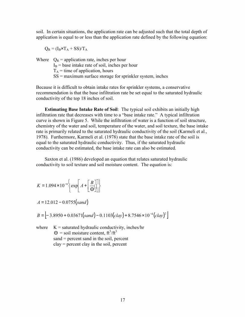
soil. In certain situations, the application rate can be adjusted such that the total depth of application is equal to or less than the application rate defined by the following equation: QR = (IB×TA + SS)/TA Where QR = application rate, inches per hour IB = base intake rate of soil, inches per hour TA = time of application, hours SS = maximum surface storage for sprinkler system, inches Because it is difficult to obtain intake rates for sprinkler systems, a conservative recommendation is that the base infiltration rate be set equal to the saturated hydraulic conductivity of the top 18 inches of soil. Estimating Base Intake Rate of Soil: The typical soil exhibits an initially high infiltration rate that decreases with time to a “base intake rate.” A typical infiltration curve is shown in Figure 5. While the infiltration of water is a function of soil structure, chemistry of the water and soil, temperature of the water, and soil texture, the base intake rate is primarily related to the saturated hydraulic conductivity of the soil (Karmeli et al., 1978). Furthermore, Karmeli et al. (1978) state that the base intake rate of the soil is equal to the saturated hydraulic conductivity. Thus, if the saturated hydraulic conductivity can be estimated, the base intake rate can also be estimated.

Saxton et al. (1986) developed an equation that relates saturated hydraulic conductivity to soil texture and soil moisture content. The equation is:

Θ

+×= − BAK exp10094.1 6

( )sandA 0755.0012.12 −=

( ) ( ) ( )[ ]24107546.81103.003671.08950.3 clayclaysandB −×+−+−=

where K = saturated hydraulic conductivity, inches/hr Θ = soil moisture content, ft3/ft3 sand = percent sand in the soil, percent clay = percent clay in the soil, percent

18

Figure 5. Example infiltration rate curve for a typical soil (from Karmeli et al., 1978) Shown in Table 1 are the soil moisture contents at saturation for various soils. The soil moisture contents are an average for each soil texture class. Fortuitously, the soil moisture content at saturation has very little variation within a soil textural class—plus or minus 5 percent or less. Once the texture of the soil is determined (percent sand, silt, and clay), the soil texture class can be determined from Figure 6. In the absence of field data, the base intake rate should be determined by using the equation developed by Saxton et al. (1986) assuming that the base intake rate is equal to the saturated hydraulic conductivity. The information needed can be obtained by finding the texture of the soil, the soil textural class (Figure 6), and the soil moisture content at saturation for the soil textural class (Table 1).

19

Table 1. Generalized soil-water characteristics based on the soil texture (adapted from Saxton, et al. 1986)

Soil Textural

Class

Percent Sand

Percent Clay

Saturated Moisture Content (ft3/ft3)

Saturated Hydraulic

Conductivity (inches/hr)

Sand 90 7 0.38 2.14 Loam Sand 82 10 0.40 1.15 Sand Loam 65 11 0.42 0.91 Sand Clay Loam

58 29 0.48 0.11

Sand Clay 50 45 0.51 0.05 Loam 43 18 0.46 0.41 Clay Loam 31 33 0.50 0.13 Clay 30 50 0.53 0.06 Silt Loam 23 16 0.47 0.64 Silt Clay Loam

12 33 0.52 0.18

Silt Clay 9 44 0.54 0.11 Silt 7 10 0.46 1.37

Interception: The most common assumption made with regard to irrigation is that all the water reaches the soil surface. Once in the soil, the water is either stored, percolates below the root zone, or is used by vegetation. Before the water reaches the soil, it must go through the plant canopy. In this process a significant percentage of the water is intercepted. There are two important concepts that must be understood. First, interception occurs for natural precipitation as well as for water applied by sprinkler irrigation. Second, plants use intercepted water to meet their cooling requirements, and the intercepted water when evaporated is considered to be part of the evapotranspiration water use. It is important to understand intercepted water because of the concern for surface runoff in OSSF systems.

Viessman et al. (1989) reported that a spruce-fir forest intercepts up to 30 percent of the precipitation. This was determined by placing rain gauges in a pasture and in a spruce-fir forest and determining the differences in the catch. Grasses and crops also intercept a significant amount of precipitation. Viessman et al. (1989) reported the annual precipitation interception rates for alfalfa, corn, soybeans, and oats to be 36, 16, 15, and 7

20

Figure 6. Soil textural triangle used to identify the class of soil (adapted from Miller and Gardner 2001). percent, respectively. In a study where 0.5 inch of water was applied in 30 minutes by a sprinkler irrigation system, the percent interception for Little bluestem, Big bluestem, Tall panic grass, Bindweed, and Buffalo grass were 50, 57, 57, 17, and 31 percent. The grass height was up to 36 inches. The conclusion that can be drawn from these data is that the vegetation will intercept a significant amount of the water applied to the spray field and thus reduce the possibility of surface runoff. It should be noted that the depth of water applied per irrigation for a typical OSSF surface application system will be 0.25 inches or less. Therefore, this application rate can occur even if the soil has a low intake rate or if the irrigation frequency is one to two days.

A concern about the plants’ use of intercepted water is often voiced. Frequently,

intercepted water is not taken into consideration in the irrigation process. However, the energy used for evapotranspiration cannot be used twice. In other words, the intercepted water will be evaporated to maintain the temperature of the plants first before the plant is required to obtain water from the soil for transpiration. The intercepted water, although never reaching the soil, is used by the system. Time of Application: The time of application as used in irrigation is the time necessary to apply sufficient water to bring the spray field up to field capacity. The soil moisture is allowed to deplete (for most practical purposes) until only 50 percent of the available soil moisture remains. Irrigation is then initiated and continued until the soil moisture in the field reaches field capacity. The length of time when the water is being applied is called the time of application (TA). There are many strategies for irrigating a field and the time of application is modified to meet the different strategies. For

21

example, a center pivot may apply 1 inch of water in 2.5 days to a field but the actual time of application may be 15 minutes due to the movement of the pivot. In a solid set system, water may be applied for only 10 minutes with frequent irrigations because of a very low water intake rate of the soil, or one may apply water for 3 hours at a rate equal to the base intake rate of the soil. The time of application is a function of evapotranspiration rates, available moisture, desired application rates, and frequency of irrigations. The determination of the proper time of application is as much art as it is a rational, calculated decision. If a soil has a relatively high intake rate and the water being applied does not hinder the application of large depths of water, the time of application can be several hours per day. Some consideration must be given to the growing environment of the crop or the continuous application of water would create the equivalent of a wetland and not a spray field. Thus the time of application is a design decision and can vary over a wide range of values and still be a sound engineering decision. Given the characteristics of OSSF systems, the time of application should not be greater than one hour per day and 0.5 hours should be used in the design process for sprinkler irrigation systems. Because of the constraints of most soils, the nitrogen content of effluents, the design flow rates of the OSSF systems, and the available effluent storage capacities, the time of application will generally be less than one hour per day. Nitrogen Control in Surface Application Systems

Prior to 1890, process efficiencies were generally evaluated on their capability to remove nitrogen in the “albuminoid” or organic form. The operating hypothesis was that nitrification represented a fermentation process (Lloyd, 1993) that was responsible for purifying wastewater, and that adequate treatment could be judged on the basis of the completeness of conversion of nitrogen to oxidized forms. The oxidation of nitrogen was believed to be the result of a “burning,” which occurred due to the presence of oxygen (Jewell and Seabrook, 1979).

The evaluation approach used considered valid at a time prior to the definition of the

nitrogen cycle. Scientific investigations concerning the role of microorganisms in nitrification and denitrification were in progress, but results of the research had not yet been applied to practical situations. Site managers knew of only one of the two major components of the nitrogen cycle and did not realize the potential for by nitrate, which is one of the oxidized forms of organic nitrogen.

Reiset (1856), as reported in Lloyd (1993), reported that decaying plant and animal

materials incessantly poured nitrogen into the atmosphere. Gayon and Dupetit confirmed Reiset’s research in 1886, and the modern era of study into denitrification began (Lloyd, 1993; Payne, 1986). Schloesing and Muntz (Payne, 1986) established the bacterial etiology of nitrification in 1877. In 1890, Winogradsky proved that nitrification is the result of chemical and biological processes mainly attributable to two specific bacteria, Nitrosomonas and Nitrococcus (Britannica, 2000).

22

The importance of the discovery of the nitrogen cycle to the agricultural and sewage

treatment communities did not become apparent for nearly fifty years. In 1940, methemoglobinemia (Sawyer et al.,1994), a blood disorder primarily affecting infants (NIANR, 1998), was discovered in the United States. Research into the illness discovered that methemoglobinemia is directly related to consumption of drinking water contaminated with high concentrations of nitrate (Canter, 1997). Muchovej and Rechcigal (1994) reported that nitrate contamination of drinking water may be linked to development of gastric cancer, non-Hodgkin’s lymphoma, increased infant mortality, central nervous system birth defects, and hypertension.

While initially attributed to excessive fertilizer use by farmers, the discovery of

nitrate contamination and its harmful effects in humans had a direct impact on surface application systems. Prior to the discovery of methemoglobinemia and its cause, hydraulic loading rates, crop requirements, soil conditions, and the nitrogen cycle were not always considered when irrigation rates were set at land treatment sites. Uncontrolled surface application of partially treated municipal wastewater caused nitrate contamination of groundwater and, in some cases, created contaminated groundwater mounds.

Modern land treatment sites are developed and operated under regulations adopted

by the EPA. Designers are now aware that compromises between engineering efficiency and crop requirements are required and that site conditions must be closely monitored to prevent groundwater contamination (Fedler and Borrelli, 1995).

The soil-plant matrix is the primary treatment mechanism in a slow-rate land

application system. The soil of the treatment plot serves as a filter for suspended solids (EPA, 1981), an environment for useful microorganisms, and a growth medium for crops. Plants protect topsoil from erosion by wind and rain, extend their roots downward into the soil to create pathways for air and water (Habib, 1988), and improve soil structure (Rose, 1991). Plants also serve as the primary removal mechanism (especially when harvested) for nitrogen (EPA, 1981).

Because of the possibility of nitrate contamination of groundwater, nitrogen is

generally considered to be the primary limiting factor in the design and operation of a slow-rate system. In arid regions, however, maintaining chlorides and total dissolved salts at acceptable levels for crop survival may be limiting (EPA, 1981; Wescot and Ayres, 1986; Oster and Rhodes, 1986). Sizing the Spray Field Land is almost always in limited supply for a spray field used to treat wastewater effluent. Thus, it is imperative to size the spray field to minimize land use. However, at all times, the spray field must be sized to meet two important criteria—the vegetation on the land must be able to assimilate the nutrients (nitrogen is usually the land limiting

23

nutrient), and the soil must be able to absorb the water without surface runoff or mounding of the water table that would create soil saturation within the root zone. The nutrient uptake by vegetation will generally control the size of the spray field. Most OSSF systems apply water to native vegetation or turf grass where the clippings are not removed. Native vegetation does not have high nitrogen uptake rates. Consequently the land area required can be much higher when nitrogen limitations are considered as compared to the land required when considering soil hydraulic limitations. To aid in the determination of the land area required for the spray field, Tables 2-4 show the nitrogen uptake rates for several different types of vegetation. Table 2. Annual nitrogen uptake rates for selected forests

Forest Trees Annual Nitrogen Uptake (lb/ac) Mixed hardwoods* 178 Red pine* 143 White spruce (old field vegetation)* 223 Pioneer succession vegetation* 223 Pulpwood** 150 Slash Pine** 190 * Overcash and Pal (1979) ** Pettygrove and Asano (1988) Table 3. Annual average nitrogen uptake rates for selected forage crops

Forage Average Annual Nitrogen Uptake (lb/ac) Alfalfa* 340 Brome grass* 158 Coastal Bermuda grass* 479 Kentucky bluegrass* 209 Quackgrass* 229 Reed canary grass* 350 Rye grass* 214 Sweet clover* 156 Tall fescue* 211 Orchard grass* 267 Bent grass** 152 Mixed pasture hay** 94 Pasture** 68 Johnson grass (regularly harvested)*** 500 Red clover*** 90 Lespedeza hay*** 116 * EPA (1981) ** Pettygrove and Asano (1988) *** Overcash and Pal (1979)

24

Table 4. Annual average nitrogen uptake rates for selected field crops Crop Average Annual Nitrogen Uptake (lb/ac)

Barley* 112 Corn* 167 Cotton* 83 Grain sorghum* 120 Potatoes* 205 Soy beans* 223 Wheat* 143 Oats (grain)* 56 * EPA (1981) Proposed Procedure To Size Spray Field: The following general procedure can be used to determine the size the spray field required for an OSSF. Step 1. Estimate the amount of nitrogen to be applied per year.

( )( )( )( )

100000036534.8QC

T nn =

where Tn is the estimated pounds of nitrogen being applied as a constituent of the wastewater, lb/yr Cn is the estimated concentration of the total nitrogen in the wastewater, mg/l Q is the estimated daily volume of water to be applied to the irrigated area, gpd The number 8.34 is the pounds of water per gallon of water The number 365 is the days per year The number 1,000,000 converts the concentration and flow rate to lbs by assuming the mg/l is the same as ppm (parts per million by weight). The total nitrogen content for aerobic and septic systems effluent can be obtained from Tables 5 and 6.

Table 5. Mean and range of effluent quality from an aerobic on-site sewage facility (Hutzler et al., 1978) Constituent Mean Range BOD SS Total N NH3-N NO3-N

65a

78a

36

0.9 30

0-208a

3-252a

15-78 0-60

0.3-72 aValues consider the additional data by various investigators cited in Hutzler et al. (1978)

25

Table 6. Mean and range of effluent quality from a septic tank on-site sewage facility (EPA, 1980) Constituent Mean Range BOD SS Total N NH3-N

139a

81a

53a

54b

7-385a

8-695a

9-125 a

49-59b

aIncludes data from Siegrist (1978). bFrom Siegrist (1978)

Step 2. Determine the spray field area based on the estimated nitrogen application rate.

( )( )

y

nn N

TArea

43560=

where Arean is the minimum required area based on nitrogen uptake by vegetation, ft2 Tn is the estimated amount of total nitrogen to be applied, lb/yr Ny is the estimated annual uptake of nitrogen by the vegetation proposed for the spray field, lb/ac/yr The number 43,560 changes the units of the area from acres to ft2. Step 3. Estimate the spray field area needed based on the estimated hydraulic

loading rate. Estimate the average daily volume applied.

48.7

QVolume =

where Volume is the estimated average daily volume to be applied, ft3/day Q is the estimated daily volume of water to be applied to the irrigated area, gpd The number 7.48 changes the volume from gallons to ft3. The next step is to estimate or choose the average time of application, TA, per day. The first choice is that the time of application should be between 0.5 and 1 hour. Next, the maximum depth of water that can be applied based on the base intake rate of the soil, IB, and the average time of application, TA, can be estimated.

12

__ ABTIdayperDepth =

where Depth_per_day is the maximum estimated depth that can be applied per day, ft/day

26

IB is the base intake rate for the soil, inches/hr TA is the average time of application, hr The number 12 is to change the depth from inches to ft. Next, the area required by the hydraulics of the system is estimated as:

dayperDepth

VolumeAreahyd __=

where Areahyd is the minimum required spray field area based on the hydraulic loading of the soil, ft2 Volume is the estimated average daily volume to be applied, ft3 Depth_per_day is the maximum estimated depth that can be applied per day, ft/day. Step 4. Select the largest area between the area required based on nitrogen (Arean)

and the area based on hydraulic loading (Areahyd). Determining Nitrogen Distribution In Irrigated Area The nutrient distribution is proportional to the effluent (or water) distribution. If the effluent contains 31 mg/l of total nitrogen and 10 inches of effluent were applied to a field, the nitrogen application would be 70 lb/acre of total nitrogen applied to the spray field. If 20 inches of effluent were applied, the nitrogen application would be 140 lb/acre. Therefore, if one can determine the distribution of effluent on the spray field, then one can also determine the distribution of nutrients. The nutrient of primary concern for an OSSF is nitrogen, especially nitrate.

Christiansen’s Uniformity Coefficient: The coefficient of uniformity is used as a measure of uniformity of water application across a field. The coefficient of uniformity is commonly determined using the Christiansen Uniformity Coefficient (UCC). This coefficient is determined by measuring the distribution of water over a typical overlapped sprinkler pattern (Figure 3). The area enclosed by four adjacent sprinkler heads is divided into 20 or more equal areas, and the depth of water on each area is measured during a typical irrigation. The equation for calculating the UCC is as follows:

1001 1 ×

×

−−=∑

=

Xn

XXUCC

n

ii

where UCC is Christiansen’s Uniformity Coefficient, percent

iX is the ith single observation depth measured, inches X is the mean of all of the individual observations, inches n is the total number of observations.

27

The recommended minimum acceptable UCC for land application of industrial and municipal wastewater is 85 percent (Borrelli, 1990). Keller and Bliesner (1990) recommend a minimum UCC of 85 percent for delicate, shallow-rooted crops when the concern is adequate moisture for crop production. Based on the distribution pattern from a single sprinkler and a sprinkler spacing (sl and sm) of 0.5 the wetted diameter, a UCC of 85 is achievable except when the distribution pattern is a “donut” shape (Pair et al., 1983) (Figure 7). A donut shape is an indication of the sprinkler head being operated at a pressure lower than recommended. Linear Distribution of Water: Karmeli et al. (1978) assessed the spatial variability of water distribution for sprinklers. With very little loss of accuracy, they found that the distribution pattern over a spray field could be modeled linearly. They developed relationships between UCC and dimensionalized depths of water. The relationships are: ( )[ ]2100100 ×−−= UCCEa

( )[ ]100/200max aEY −= [ ]100/min aEY = where Ea is the water application efficiency in percent UCC is the Christiansen Uniformity Coefficient in percent Ymax is the actual depth applied divided by the average depth applied (field average) on that part of the spray field receiving the most water Ymin is the actual depth applied divided by average depth applied (field average) on that part of the spray field receiving the least amount of

water. The above relationships assume that the depth of application varies linearly with the fraction of area for the spray field and that the depth of application is equal to the depth of water needed to bring the soil moisture up to field capacity.

28

Figure 7. Coefficient of uniformity for various sprinkler discharge profiles (Pair et al., 1983) An estimate can be made as to the depth of water applied to all parts of the field. A linear non-dimensional distribution curve for depth can be developed if the fraction of area receiving the various depths is arranged from smallest to highest. The equation is: ( ) ( )[ ]XYYYY ×−+= minmaxmin where Y is the dimensionless depth or actual depth divided by the average depth applied (field average) X is the fraction of area having a dimensionless depth of Y or less Ymax is the actual depth applied divided by the average depth applied (field average) on that part of the spray field receiving the most water Ymin is the actual depth applied divided by average depth applied (field average) on that part of the spray field receiving the least amount of

water. The value of X will vary from 0.0 to 1.0 with X = 0.5 occurring at Y =1 (an example is shown in Figure 8). Using the above equations, the distribution of water over a field can be estimated by knowing the UCC of the sprinkler system. The UCC must be measured or estimated. Because the distribution of water is critical to the proper distribution of wastewater constituents, a UCC of at least 85 percent is preferred for the spray field of the OSSF.

29

When the depth of water applied is less than the depth needed to bring the spray field to field capacity, the value for Ea will increase. However, the distribution of water over the spray field remains the same and UCC does not change except due to shifts in wind. Regardless, water is applied deeper than average on some parts of the spray field and less than average on other. For a given irrigation system, the same parts of the spray field are over-irrigated or under-irrigated for each irrigation. This also means that nutrients or other land-limiting constituents will also be applied at greater and lesser amounts than average. Example for Using the Coefficient of Uniformity: The following example is provided to demonstrate the need for a properly designed sprinkler irrigation system. Too often, current practice is to provide no overlap of sprinklers. Thus the distribution pattern is that provided by a single sprinkler. For this example, it is assumed that the distribution pattern is triangular or a truncated cone in three dimension. Volume of wastewater per day: 300 gpd Total nitrogen content in wastewater: 30 mg/l Maximum application rate for surface irrigation of treated effluent: 0.041 gal/ft2/day (TAC 285.90, 2001) Vegetation: Pioneer succession vegetation Nitrogen uptake of vegetation: 223 lb/yr Land limiting factor: nitrogen Christiansen Uniformity Coefficient: 85 percent Wetted diameter of sprinkler head: 20 ft Calculations: Proposed Method Cn = 30 mg/l Q = 300 gpd Ny = 223 lb/yr

( )( )( )( )1000000

36534.8QCT n

n = ; Tn = 27.40 lb/yr

( )( )

y

nn N

TArea

43560= ; Arean = 5,352 ft2

36548.7

×= QVolume ; Volume = 14,639 ft3

12_ ×=nArea

VolumeAppliedDepth ; Depth_Applied = 32.76 inches/yr

Assume UCC = 85

30

( )[ ]2100100 ×−−= UCCEa Ea = 70 ( )[ ]100/200max aEY −= Ymax = 1.30 [ ]100/min aEY = Ymin = 0.70 Thus, 50 percent of the irrigated area has an average annual application of 1.15 time the depth applied per year, that is, this portion of the field was over-irrigated (Figure 8).

0

0.20.4

0.6

0.8

11.2

1.4

0 0.1 0.2 0.3 0.4 0.5 0.6 0.7 0.8 0.9 1 1.1

Fraction of Area (X)

Dim

ensi

onle

ss P

reci

pita

tion

Dep

th (Y

)

Figure 8. Estimated linear distribution of water on field irrigated with wastewater effluent. The volume of water applied to the 50 percent of the irrigated area that was over irrigated was Volume50 = 14,639×1.15×0.5 = 8417 ft3 Amount of nitrogen applied: Napplied = 27.4×0.5×1.15 = 15.76 lb/yr Amount of nitrogen used by the selected vegetation:

223435602

5352 ××

=usedN ; Nused = 13.75 lb/yr

Amount of nitrogen leached is: Nleached = 15.76 – 13.75 = 2.01 lb/yr

31

Calculations: Current TAC 285 Method Cn = 30 mg/l Q = 300 gpd Ny = 223 lb/acre/yr

( )( )( )( )1000000

36534.8QCT n

n = Tn = 27.40 lb/yr

36548.7

×= QVolume Volume = 14,639 ft3

7317041.0

300 ===MAR

QArea ft2

12_ ×=Area

VolumeAppliedDepth ; Depth_Applied = 24.01 inches/yr

To estimate the fate of the nitrogen within this system, it was necessary to select a typical sprinkler system and its appropriate shape of water distribution. In this case, a 40 ft wetted diameter sprinkler was used and the water distribution pattern form an individual sprinkler is assumed to be a typical truncated cone-shaped pattern. The area affected by this sprinkler was sub-divided into 24 equal concentric parts in order to estimate the amount of nitrogen being applied beneath the sprinkler. With the truncated cone pattern, the average depth of water applied to each of the 24 sub-areas was determined (Table 7). Based on that incremental depth of water applied, the annual amount of nitrogen applied was determined. Lastly, the amount of deficit or excess nitrogen applied to the site was determined by subtracting the amount of plant uptake nitrogen (0.268 lb N) from the incremental nitrogen applied. The following data were selected or determined for a single sprinkler head considering the assumptions stated for this example case study. Wetted Diameter of Sprinkler: 40 ft Area Covered by Sprinkler: 1256.6 ft2 Average Depth of Water: 24.01 in. Volume of water per year: 2514 ft3 Total Nitrogen Applied 4.71 lb/yr Nitrogen per Inch of Water: 0.196 lb/ac-in of water applied over the 1256.6 ft2 Crop Nitrogen Use: 6.433 lb/yr

32

Table 7. Estimated annual nitrogen distribution over the area covered by a single sprinkler head Number of Area Average Depth of

Water Applied for incremental area, in.

Incremental Nitrogen Applied,

lb

Deficit (-) or Excess Nitrogen

Applied, lb 1 0.76 0.0062 -0.2618 2 2.29 0.0187 -0.2493 3 3.86 0.0315 -0.2365 4 5.46 0.0446 -0.2235 5 7.11 0.0581 -0.2100 6 8.79 0.0718 -0.1963 7 10.53 0.0860 -0.1820 8 12.31 0.1005 -0.1675 9 14.15 0.1156 -0.1525 10 16.05 0.1311 -0.1370 11 18.01 0.1471 -0.1210 12 20.05 0.1637 -0.1043 13 22.18 0.1811 -0.0869 14 24.40 0.1993 -0.0688 15 26.72 0.2182 -0.0498 16 29.18 0.2383 -0.0297 17 31.78 0.2595 -0.0085 18 34.57 0.2823 0.0143 19 37.58 0.3069 0.0389 20 40.88 0.3339 0.0658 21 44.59 0.3642 0.0961 22 48.89 0.3993 0.1312 23 54.27 0.4432 0.1752 24 64.67 0.5281 0.2601

Total 4.731 0.782* *Sum of positive values in the column Based on the above analysis, this individual sprinkler head had excess water applied on 7 of the 24 incremental sub-areas, or 29.2 percent of the area beneath this sprinkler received excess water. This excess water resulted in excess nitrogen being applied at a rate of 0.782 lb over this incremental area or an equivalent of 93 lb/ac/yr. Note that this excess nitrogen applied only occured on the area receiving the excess water. From the 7317 ft2 of irrigated area required by the design, the number of sprinklers required to cover the total area was 5.8 sprinklers. Since the total excess nitrogen applied per sprinkler was 0.782 lb, these sprinklers applied a total of 4.55 lb of excess nitrogen to the site, which will be prone to be leached below the root zone of the crop. This 4.55 lb of nitrogen represents 16.6 percent of the nitrogen applied compared to only 7.3 percent of excess nitrogen applied with the proposed design method. Another fact to note is that the effluent was applied at approximately 46 percent of the rate of evapotranspiration on 37

33

percent more land than is required by the proposed method of designing a sprinkler system where 63 percent of the crop water use is provided. If the western part of the state is considered, where the maximum application rate as prescribed in TAC 285.90 increases to 0.115 gal/ft2/day, the area required would decrease to 2609 ft2 for the same effluent quantity of 300 gpd. When using a sprinkler system designed with no overlap, there would be approximately 16 lb of nitrogen leached below the root zone or 59 percent of the nitrogen applied. The area receiving excess nitrogen would increase from 29.2 percent of the area to 71 percent of the irrigated area. In this case, 51 percent of the crop water use was provided with the proposed method, whereas 105 percent was provided by the TAC 285.90 method. For the proposed method of sizing a spray field, the percent of the applied nitrogen leaching below the root zone would remain at 7.3 percent for any location in the state. The quantity of nitrogen that could potentially reach the groundwater from a single OSSF may appear to be quite small, but there are two other factors that need to be considered. First is the total number of OSSF’s installed in the state and the subsequent total mass of nitrogen that could reach our water resources. The second component that needs to be considered is the number of home clusters that exist, especially those that surround the many lakes that the population uses for recreation. If the mass of nitrogen can be reduced from 7 to 52 percent by adopting this proposed method of designing surface application systems for OSSFs, both our fresh water drinking supplies and our recreational lakes will be maintained at a much higher quality.

These examples considered are using the truncated cone shaped water distribution pattern only, and the results will change when another distribution pattern is considered or if overlap of the sprinklers is designed into the system. In addition, no surface application system should be designed on only one parameter when there are numerous factors to consider, each affecting the outcome of the other. A sound design will always consider both a water balance and a nutrient balance on the system. Recommendations

The surface application rates for Texas OSSF have been evaluated and a new method has been proposed. It is recommended that the following changes be made to the current Texas Administrative Code 285 rules in order to provide for the least amount of negative impact our the states environment. 1. All surface application systems designed for an on-site sewage facility should

consider both a water balance and a nutrient balance for the final design. 2. The layout of the site for effluent application should be in a block pattern such that

the sprinklers can be arranged to have a head-to-head overlap. If this is not available, then the system should be designed such that the proper overlap can be provided in order to achieve a uniformity coefficient of 80 percent or greater.

34

3. Spray head type of sprinklers should not be used in an OSSF system while the gear head type should be used.

4. All sprinklers are designed to operate at an optimum pressure range to obtain the specified pattern of water distribution and the OSSF design pressure should be in the middle of the specified range of the chosen sprinklers. Sprinklers operating at pressures lower or higher than designed will produce unreliable patterns that will result in unacceptable water application efficiencies.

5. The time used to apply the effluent should not exceed 1 hour and the average design should be 0.5 hours.

6. The base water intake rate of the soil should follow that described by Saxton et al. (1986) provided more precise information on the soil is not available.

7. The base soil infiltration rate should be set equal to the saturated hydraulic conductivity of the top 18 inches of soil.

8. A check-off list of design considerations (see below) should be developed and used on all new and renovated designs of OSSF where surface application of the effluent is utilized.

List of Design Considerations

In order to check the design of any surface application system for OSSF’s, several design considerations need to be examined that are common to practically all systems. The following is a list of design considerations that should be examined for all designs. 1. Sprinklers should be spaced such that their spray pattern reaches an adjacent sprinkler

(called head-to-head spacing). 2. The pressure difference between the sprinkler with the highest pressure and the

sprinkler with the lowest pressure in a set should be less than 20 percent. 3. The discharge rate between the sprinkler with the lowest rate and the sprinkler with

the highest rate for a set should be less than 10 percent. 4. The uniformity coefficient for any sprinkler set should be 80 percent or greater. 5. Risers of 6 inches should be used when the discharge rate is less than or equal to 12

gpm and the risers should be 12 inches for discharge rates between 12 and 26 gpm. 6. The application rate of the effluent should be less than or equal to the base intake rate

of the soil plus 0.1 inches to account for interception.

35

References Borrelli, J. (1990). “Land Application of Industrial and Municipal Wastewater.” Paper

presented at the 1990 meeting of the American Society of Agricultural Engineers, Texas Section, College Station, Texas. 10 pages.

Britannica.com. (2000). “Winogradsky, Sergey Nikolayevich.”

http://www.britannica.com/seo/s/sergey-nikolayevich-winogradsky/ EPA. (1980). “Design Manual—Onsite Wastewater Treatment and Disposal Systems.”

U.S. Environmental Protection Agency, Center for Environmental Research Information, Cincinnati, Ohio, pgs. 121, 149, 282.

EPA. (1981). “Process Design Manual—Land Treatment of Municipal Wastewater.”

EPA-625/1-81-013. U.S. Environmental Protection Agency, Center for Environmental Research Information, Cincinnati, Ohio.

Fedler, C. B. and Borrelli, J. (1995). “Designing For Optimum Land Application

Systems.” Presented at the International Summer Meeting of the ASAE. Chicago, IL. June 18-23. Paper No. 952407. ASAE, 2950 Niles Road, St. Joseph, MI 49085-9659. USA.

Habib, A., Zartman, R.E., and Ramsey, R.H. (1988). “Intrapedal Macropore

Distribution and Infiltration rate of Three Friona Polypedons.” Soil Science, 145 (4), 244-249.

Hutzler, N. J., Waldorf, L.E., and Fancy, J. (1978). “Performance of Aerobic Treatment

Units.” Proceedings of the Second National Home Sewage Treatment Symposium. St. Joseph, MI. pgs. 149-163.

Jensen, M. E. (1983). Design and Operation of Farm Irrigation Systems. American

Society of Civil Engineers. St. Joseph, Michigan. 829 pages. Jensen, M. E., and Burman, R.D., and Allen, R.G.. (1990). Evapotranspiration and

Irrigation Water Requirements. ASCE Manuals and Reports on Engineering Practice No. 70. American Society of Civil Engineers. New York. 332 pages.

Jewell, W.J. and Seabrook, B.L., 1979. A History of Land Application as a Treatment

Alternative. United States Environmental Protection Agency, Office of Water Program Operations, Washington, D.C. 20460.

Karmeli, D., Salazar, L.L., and Walker, W.R.. (1978). “Assessing the Spatial Variability

of Irrigation Water Applications.” EPA-600/2-78-041. U.S. Environmental Protection Agency, Robert S. Kerr Environmental Research Laboratory. Ada, Oklahoma.

36

Keller, J. and Bliesner, R.D. (1990). Sprinkler and Trickle Irrigation. avi Book, Van Nostrand Reinhold, New York. 652 pages.

Lloyd, D. (1993). “Aerobic Denitrification in Soils and Sediments: From Fallacies to

Facts.” Tree, 8(10), 352-355. Miller, R.W. and Gardner, D. T. (2001). Soils in Our Environment. Prentice Hall, Upper

Saddle River, New Jersey, 642 pages. Muchovej, R.M.C., and Rechcigl, J.E. (1994). “Impact of Nitrogen Fertilization of

Pastures and Turfgrasses on Water Quality,” in Soil Processes and Water Quality, Lal, R. and Stewart B.A., editors. Lewis Publishers, Boca Raton, Fl. 113-114.

NIANR (1998). Drinking Water: Nitrate and Methemoglobinemia (“Blue Baby”

Syndrome), G98-1369. University of Nebraska, Institute of Agriculture and Natural Resources (NIANR).

Oster, J.D. and Rhoades, J.D. (1986). “Water Management for Salinity and Sodicity

Control,” in Irrigation With Reclaimed Municipal Wastewater—A Guidance Manual, Pettygrove, G.S. and Takashi, A., editors. Lewis Publishers, Chelsea, MI. Chapter 7.

Overcash, M. R., and Pal, D. (1979). Design of Land Treatment Systems for Industrial

Wastes: Theory and Practice. Ann Arbor Science, Ann Arbor, Michigan. 684 pages. Pair, C. H., Hinz, W.H., Frost, K.R., Sneed, R.E., and Schiltz, T.J. (1983). Irrigation. The

Irrigation Association. Silver Spring, Maryland. 686 pages. Payne, W.J. (1986). “1986: Centenary of the Isolation of Denitrifying Bacteria.” ASM

News, 52(12), 627-629. Pettygrove, G. S. and Asano, T. (1985). Irrigation with Reclaimed Municipal

Wastewater—A Guidance Manual. Luis Publishers, Chelsea, Michigan. Rose, D.A. (1991). “Organic Matter and Soil Structure,” in Advances in Soil Organic

Matter Research: The impact on Agriculture and the Environment, Wilson, W.S., editor. The Royal Society of Chemistry. Cambridge. 139.

Sawyer, C.N., McCarty, P.L., and Parkin, G.F. (1994). Chemistry for Environmental

Engineering. 556-557. Saxton, K. E., Rawls, W.J., Romerger, J.S., and Papendick, R.I. (1986). “Estimating

Generalized Soil-water Characteristics from Texture.” American Society of Soil Science Journal. Vol. 50, pages 1031-1036.

37

Siegrist, R. L. (1978). “Waste Segregation to Facilitate On-site Wastewater Disposal Alternatives.” Proceedings of the Second National Home Sewage Treatment Symposium. St. Joseph, MI. pgs. 271-281.

Viessman, W., Jr., Lewis, G.L., and Knapp, J.W. (1989). Introduction to Hydrology.

Harper & Row, Publishers, New York. 780 pages. Wescot, D.W. and Ayres, R.S. (1986). “Irrigation Water Quality Criteria,” in Irrigation

With Reclaimed Municipal Wastewater—A Guidance Manual, Pettygrove, G.S. and Takashi, A., editors. Lewis Publishers, Chelsea, MI. Chapter 3.

38

Glossary Application Rate: The amount of water applied to a given area measured in inches per hour. Available Soil Moisture: Water in the root zone that can be extracted by plants. The available soil moisture is the difference between field capacity and wilting point (Hill, 1994). Basic Intake Rate: The almost constant rate that a soil will take in water after large cracks, pores and cavities are filled. Consumptive Use: The total amount of water taken up by vegetation for transpiration or building of plant tissue, plus the unavoidable evaporation of soil moisture, snow, and intercepted precipitation associated with vegetal growth; synonymous with evapotranspiration (Jensen et al., 1990). Distribution Pattern: The pattern of water application by a sprinkler over the area the sprinkler covers. The area is generally circular in form; synonymous with sprinkler pattern. Evapotranspiration: The combined processes by which water is transferred from the earth surface to the atmosphere; evaporation of liquid or solid water plus transpiration from plants (Jensen et al., 1990). Field Capacity: The moisture content of a soil following an application of water and after the downward movement of excess water (from gravitational forces) has essentially ended. Usually it is assumed that this condition is reached about two days after a full irrigation or heavy rain (Hill, 1994). Head to Head Spacing: Spacing of sprinklers so that the radius of the sprinkler match the spacing of the sprinklers. Also referred to a 100 percent coverage, head to head coverage or 100 percent overlap. Irrigation Frequency: The maximum number of days that can be allowed between irrigations during periods of peak water use, without causing plants to suffer. Rainfall can change irrigation frequency requirements. Irrigation Period: Refers to the number of days used to apply irrigation water in the volume needed for a given area during the peak consumptive water use period of the crop being irrigated. Lateral Lines: The lines equipped with sprinkler heads.

39

Leaching: The process of water movement through and below the crop root zone by gravitation. It occurs whenever the infiltrated irrigation water and rainfall exceed the crop evapotranspiration and the water storage capacity of the soil profile (SCS, 1993). Main Lines: In sprinkler irrigation, they are the lines that convey the water from the supply line or water source to the lateral lines. Operating Pressure Range: The range from minimum to maximum pressure under which the head will deliver designed distribution of water throughout it’s entire area of coverage. Overlap: The amount one sprinkler pattern overlaps another sprinkler pattern when installed in a specific pattern. Usually expressed as a percentage of the. Radius or Diameter of Throw: The actual distance, determined by the manufacture’s testing, that a sprinkler head will spread water. Riser: A length of pipe, affixed to a lateral line, sub-main or main water line, for the purpose of supporting a valve or sprinkler head; diameters of risers are normally less than that of the pipe-line and in the case of sprinklers should be from six inches to several feet in length to counteract the effect of turbulence caused when water is diverted from its original direction of flow. A nipple to which the sprinkler is attached. Root Zone: The depth to which plant roots invade the soil and where water extraction occurs (Hill, 1994). Section: (noun) A group of heads and/or valves that operate as one station or a controller or at one time on a manual system. Sets: Any area of a field that can be supplied water until the soil profile requirements are met and not exceeded before changing or moving the apparatus used for distributing or applying the irrigation water. Underspaced: The unusual situation in which sprinkler heads are spaced closer than required for efficient operation of the system. Wall-to-Wall Coverage: Indicates complete coverage of the area to be irrigated from one border to the other. This requires part circle border sprinkler heads for total coverage. Water Application Efficiency: The ratio of the average depth of irrigation water infiltrated and stored in the root zone to the average depth of irrigation water applied, expressed as a percentage. Wilting Point: The soil moisture content at which a plant can no longer obtain sufficient moisture to satisfy its requirements and, therefore, will wilt permanently (Hill, 1994).

40

Appendix

Example OSSF Designs

Design of Sprinkler System for a 375 gpd System

The following condition are for a single family dwelling with four bedrooms, less than 3,500 square ft., and without water saving devices.

Flow rate: Q 375:= gpdQ is the estimated daily volume of water to be applied, gal/day

Base intake rate of soil IB 0.15:= inches/hrIB is base intake rate (minimum) for the soil, inches/hr

Crop: Mixed grasses and sweet clover

Nitrogen uptake: Ny 130:= lb/ac/yr "Estimated"This assumes no denitrification and no harvest of plant material.

Ny is the estimated annual uptake of nitrogen by the vegetation proposedfor the spray field, lb/ac

Total N in water: Cn 30:= mg/lCn is estimated concentration of total nitrogen in the wastewater effluent, mg/L

Elevation difference between the pump and the spray field: SL 12:= ftSL is the elevation difference between the pump and the spray field, ft

Distance from pump to spray field: L 300:= ftL is the distance from the pump to the spray field or connection to the main line, ft

Desired operating pressure at sprinkler heads: Pd 30:= psiPd is the desired operating pressure for the chosen sprinklers, psi

Desired sprinkler spacing: Sl 30:= ft Sm 30:= ft

41

sl is the sprinkler spacing along the lateral, ftsm is the sprinkler spacing along the main, ft

Maximum surface storage on soil: SS 0.2:= inchesMaximum surface storage for the applied water, inches

Volume of storage tank: Vol 750:= galVol is the volume of the storage tank between the alarm-on level and thepump-on level, gal

It is recommended that the storage tank volume be 2 times the average daily volume of water, Q.

Design Steps:Step 1. Determine the amount of nitrogen being applied per year.

TnCn Q⋅ 8.34⋅ 365⋅

1000000:= Tn 34.246= lb/yr

Tn is the estimated pounds of total nitrogen being applied as a constituentof the wastewater effluent, lb/yr

Step 2. Determine the spray field area based on nitrogen application rate.

AreanTn

Ny43560⋅:= Arean 1.148 104×= ft2

Arean is the minimum area of the spray field assuming nitrogen is theland-limiting factor, ft2

Step 3. Determine the Required area based on hydraulic loading rate.

Assume the daily average time of application is 30 minutes: TA 0.5:= hr

TA is the time of application of effluent on to the spray field, hr

The value for TA was assumed reasonable for an OSSF system. TA could beas long as 5 hours according to TNRCC regulations--285.33.

42

Step 6. Layout blocks and sprinkler heads (see Figure 375A)

Determining the number of spray blocks merely helps in the decision onhow to lay out the spray field--number of laterals and sprinkler heads perlateral.

Nosb is number of spray blocks needed for the spray field system.

A spray block is the area encompasssed by sl times sm. Use 14

Nosb 13=Nosb trunc Nosb 1+( ):=NosbAreaSl Sm⋅

:=

Step 5. Determine the number of spray blocks--use even number.

ft2Area 1.148 104×=Area Arean:=

Step 4. Select the largest of the area in Step 2 and Step 3.

Areahyd is the minimum area of the spray field assuming the intake rate of the soil or the hydraulic loading rate is the land-limiting factor, ft2

ft2Areahyd 8.021 103×=AreahydVol_per_day

Depth_per_day:=

ft/dayDepth_per_day 6.25 10 3−×=Depth_per_dayIB TA⋅

12:=

ft3/dayVol_per_day 50.134=Vol_per_dayQ

7.48:=

43

This sprinkler head discharge rate is based on allowing an adjustmentfor the surface storage and should be considered a maximum value.

gpmQspr 5.14=QsprQR Sl⋅ Sm⋅

96.3:=

QR is the maximum application rate adjusted for surface storage and timeof application, inches/hr

inches/hrQR 0.55=QRIB TA⋅ SS+

TA:=

Step 8. Determine maximum sprinkler discharge based on TA and SS.

Qspr is the discharge rate from a full-circle sprinkler head, gpm

gpmQspr 1.402=QsprIB Sl⋅ Sm⋅

96.3:=

Step 7. Determine maximum sprinkler discharge for a full circle sprinkler head based on the base intake rate of the soil, IB.

Figure 375A.- Preliminary Layout of Sprinkler System

Note the full, half and quarter circle sprinklers heads used in this block.

44

Step 9. Select the sprinkler head--this may require a change in the operating pressure at the sprinkler head and the sprinkler spacing. This will require modifications to Steps 1-8.***********************************************************************************

This is where the design of a sprinkler system for an OSSF system differsfrom the design of a turf irrigation system. When designing a turf irrigationsystem, one is concerned with replenishing water in the soil profile and applying 1 to 2 inches of water per irrigation. In this case, the design should make sure the application rate does not exceed the base intake rate of thesoil plus the interception or there could be surface runoff.

However, for an OSSF system, the irrigation frequency is usually everyday and the depth of application will generally be less than 0.25 inches ofwater. The actual time of application will be small and the intake rate willalmost always be greater than the base intake rate because it takes timefor the intake rate to decrease to the base intake rate. Furthermore, one can take advantage of surface storage and apply water at a rate somewhat greater than the base intake rate.

With the above considerations in mind, an application rate could be very smallor large enough so that the maximum discharge from the sprinker isachieved as calculated in Step 8. Thus for this design, one could selecta full circle sprinkler discharge rate from something near 2 gpm to 5.14 gpm and still have an acceptable design.

After a review of various commercial sprinkler heads, a discharge rate of4 gpm was selected for a full-circle sprinkler head.

***********************************************************************************

Use K-rain Dial-a-nozzle 12 deg low angle, operated at 30 psi.

nozzle #1 Dw = 60 ft Qspr = 1.0 gpm Use for quarter-circlenozzle #2 Dw = 64 ft Qspr = 2.0 gpm Use for half-circlenozzle #4 Dw = 64 ft Qspr = 4.0 gpm Use for full-circle

The 4.0 gpm is less than the maximum 5.12 gpm determined inStep 8. The wetted diameter (Dw) is acceptable.

Dw is the wetted diameter for the given orifice and operating pressure.

45

The above appears to be a reasonable time to drain a full tank. The timeneeded is less than the 5 hour window for application required by TNRCC-285.33

Time to drain full tank TdVolQset

:= Td 26.786= min

Number of sets Noset 2:=For this design, the two outside lateralswill be one set and the middle lateralwill be the second set. Each set willdischarge 28 gpm.

gpm Qset 28=Qset2 Qendlat⋅ 1.0 Qmidlat⋅+( )

2:=

The average discharge per set is.

Step 12. Determine the irrigation sets or sections for the spray field.

Qmidlat is the total flow into the middle lateral(s) of the proposed sprinklersystem, gpm.

Qendlat is the total flow into the end laterals of the proposed spinkler system, gpm.

Note: 6(2) + 2(1) = 14 and 6(4) + 2(2) = 28

gpm Qmidlat 28:=gpm Qendlat 14:=

Step 11. Determine the total discharge for all sprinklers from each lateral. Use Figure 375A.

Actual application rate is less than the maximum application rate, QR providedTA remains as assumed, therefore allowable.

inches/hr App_rate 0.428=App_rateQspr 96.3⋅

Sl Sm⋅:=

Step 10. Check application rate for selected sprinkler head. Use the flow rate for the full circle sprinkler head.

gpm, as stated above Qspr 4:=

46

TsetTd

Noset:= Tset 13.393= min

The time of application, TA, is equal to the Tset.

It is recommended that the set time be 14 minutes for this system.

Tset 14:= min

TA Tset:=

Step 13. Layout the pipe, sprinkler heads, control valves, and connection to the supply line (see Figure 375B).

Figure 375B.-Layout of sprinkler heads and control valves.

Step 14. Size the laterals. There must be less than 20 percent pressure loss along the lateral. Calculate the pressure loss starting with the last segment of pipe (attached to the last sprinkler head) and go to the control valve. Sum the headloss in each segment to obtain the total headloss in the lateral.

Roughness of pipe C 140:= Use sch 40 PVC pipe.

C is the Hazen-Williams pipe roughness factor for PVC pipe.

Laterals 1 and 3 are the same.

47

Qsegn

261014182226

:=Lsegn

30303030303030

:=Segmentn

1234567

:=

inches inside diameterD 1.380:=n 0 6..:=

Headloss for Lateral 2 or middle lateral using nominal 1.25 inch PVC pipe.

psi totalhf 3.698=totalhftotalhf2.31

:=ft totalhf 8.541=

totalhf

0

6

n

hfsegn∑=

:=hfsegn

Lsegn 3.0226⋅Qsegn

π D2⋅ 448.9⋅4 144⋅

1.852⋅

C1.852 D12

1.167⋅

:=

Hazen-Williams formula for friction loss in a pipe.

Segment is the pipe segmentalong the lateral starting with the last sprinkler head.

Lseg is the length of each segmentin feet.

Qseg is the flow rate within eachsegment in gpm.

Qsegn

135791113

:=Lsegn

30303030303030

:=Segmentn

1234567

:=D is the inside diameter of the pipe in inches

inches inside diameterD 1.049:=n 0 6..:=Headloss for Laterals 1 and 3.

48

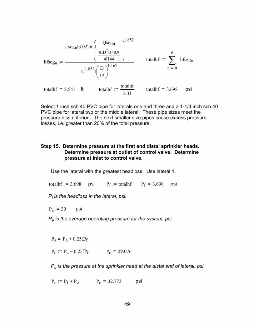
psi Pn 32.773=Pn Pf Po+:=

Po is the pressure at the sprinkler head at the distal end of lateral, psi.

Po 29.076=Po Pa 0.25 Pf⋅−:=

Pa Po 0.25 Pf⋅+=

Pa is the average operating pressure for the system, psi.

psi Pa 30:=

Pf is the headloss in the lateral, psi.

psiPf 3.698=Pf totalhf:=psi totalhf 3.698:=

Use the lateral with the greatest headloss. Use lateral 1.

Step 15. Determine pressure at the first and distal sprinkler heads. Determine pressure at outlet of control valve. Determine pressure at inlet to control valve.

Select 1 inch sch 40 PVC pipe for laterals one and three and a 1-1/4 inch sch 40 PVC pipe for lateral two or the middle lateral. These pipe sizes meet the pressure loss criterion. The next smaller size pipes cause excess pressure losses, i.e. greater than 20% of the total pressure.

psi totalhf 3.698=totalhftotalhf2.31

:=ft totalhf 8.541=

hfsegn

Lsegn 3.0226⋅Qsegn

π D2⋅ 448.9⋅4 144⋅

1.852⋅

C1.852 D12

1.167⋅

:= totalhf

0

6

n

hfsegn∑=

:=

49

Lenget of main line, L30, is set at 30 ft.

gpmQ30 14:=ft L30 30:=inches inside diameterD 1.049:=

The supply line will discharge into the middle of the main line.

Step 16. Determine the size of the main line. The pressure loss in the main should be less than 10 percent of the average operating pressure of the sprinkler system.

psi Pvalve_inlet 38.282=Pvalve_inlet Pvalve_outlet PLvalve+:=

psi PLvalve 4.5:=

Pressure loss in valve, PLvalve, is found from manufacturers catalog.

psi Pvalve_outlet 33.782=Pvalve_outlet Pnhf20

2.31+:=

ft hf20 2.33=hf20

L20 3.0226⋅Q20

π D2⋅ 448.9⋅4 144⋅

1.852

⋅

C1.852 D12

1.167⋅

:=

gpm Q20 14:=ft L20 20:=inches inside diameterD 1.049:=

There is 20 feet of 1-inch pipe to control valve.

Pn is the pressure at the first sprinkler head on the lateral, psi.

50

psi Ppump_outlet 50.911=

Ppump_outlethfsupply

2.31Psupply+

SL2.31

+:=

ft hfsupply 15.659=hfsupply

L 3.0226⋅Q

π D2⋅ 448.9⋅4 144⋅

1.852⋅

C1.852 D12

1.167⋅

:=

Flow rate for set requiring the highest flow rate.gpm Q 28:=

C 140:=inches D 1.610:=ft L 300=

Use a 1-1/2-inch sch 40 PVC pipeline or the same pipe size used for the main line.

Step 17. Calculate the headloss in the supply line.

psi Psupply 38.937=Psupply Pvalve_inlethf30

2.31+:=

The pressure at the supply line, Psupply (psi), is

Pressure loss in main is less than 10 percent of operating pressure.A 1 inch sch 40 pvc pipe will serve as the main for lateral 1 and 3.

psi hf30 1.513=hf30hf30

2.31:=hf30 3.495=

hf30

L30 3.0226⋅Q30

π D2⋅ 448.9⋅4 144⋅

1.852

⋅

C1.852 D12

1.167⋅

:=

51

K 19=

K

0

10

u

kvalueu∑=

:=

kvalueu

1.20.29.32.20.21.30.70.71.70.51.0

:=itemu

"solenoid valve""gate valve""strainer""check valve""union""tee""90 deg elbow""90 deg elbow""foot valve""entrance""exit"

:=

u 0 10..:=

Calculate the minor losses in the system.

fpsVsupply 4.412=VsupplyQ

π D2⋅ 448.9⋅4 144⋅

:=Velocity in supply line

Diameter of supply lineD 1.61=

Note: the 448.9 is a conversion factor,The 144 converts in2 to ft2

psi hfsuc 0.134=hfsuchfsuc

2.31:=hfsuc

Lsuc 3.0226⋅Q

π Dsuc2⋅ 448.9⋅

4 144⋅

1.852⋅

C1.852 Dsuc

12

1.167⋅

:=

Diameter of suction pipe is one size largerthan the supply pipe line.

gpm Q 28:=inches Dsuc 2.067:=C 140:=ft Lsuc 20:=

Step 18. Calculate minor losses and headloss in suction pipe.

52

PLminor KVsupply

2

2 32.2⋅⋅

12.31

⋅:= PLminor 2.486= psi

Step 19. Calculate Total Dynamic Head

TDH PLminor hfsuc+( ) 2.31⋅ Ppump_outlet 2.31⋅+:=

TDH 123.656= ft TDHTDH2.31

:= TDH 53.531= psi

Need a pump that will pump 28 gpm at 147 ft of TDH.

53

Design of Sprinkler System for a 1200 gpd System

The following condition are assumed for 2-single family dwellings (four bedrooms) less than 3,500 square feet (375 gpd per dwelling) and 1-single family dwelling (five bedrooms) less than 4,500 square feet (450 gpd). All dwellings are without water saving devices.

Flow rate: Q 1200:= gpdQ is the estimated daily volume of water to be applied, gal/day

Base intake rate of soil IB 0.20:= inches/hrIB is base intake rate (minimum) for the soil, inches/hr

Crop: Pulpwood

Nitrogen uptake: Ny 150:= lb/ac/yr This assumes no denitrification and no harvest of plant material.

Ny is the estimated yearly uptake of nitrogen by the vegetation proposedfor the spray field, lb/ac/yr

Total N in water: Cn 30:= mg/lCn is estimated concentration of total nitrogen in the wastewater effluent, mg/l

Elevation difference between the pump and the spray field: SL 20:= ftSL is the elevation difference between the pump and the spray field, ft

Distance from pump to spray field: L 500:= ftL is the distance from the pump to the spray field or connection to main line, ft

Desired operating pressure at sprinklers: Pd 30:= psiPd is the desired operating pressure for the chosen sprinklers, psi

Desired sprinkler spacing: Sl 30:= ft Sm 30:= ft

54

sl is the sprinkler spacing along the lateral, ftsm is the sprinkler spacing along the main, ft

Maximum surface storage on soil: SS 0.2:= inchesMaximum surface storage for the applied water, inches

Volume of storage tank: Vol 2400:= galVol is the volume of the storage tank between the alarm-on level and thepump-on level, gal

It is recommended that the Vol be 2 times the average daily volume of water, Q.

Step 1. Determine the amount of nitrogen being applied per year.

TnCn Q⋅ 8.34⋅ 365⋅

1000000:= Tn 109.588= lb/yr

Tn is the estimated pounds of total nitrogen being applied as a constituentof the wastewater effluent, lb/yr

Step 2. Determine the spray field area based on nitrogen application rate.

AreanTn

Ny43560⋅:= Arean 3.182 104×= ft2

Arean is the minimum area of the spray field assuming nitrogen is theland-limiting factor, ft2

Step 3. Determine the required area based on hydraulic loading rate.

Assume the daily average time of application is 30 minutes: TA 0.5:= hr

TA is the time of application of effluent on to the spray field, hr

The value for TA was assumed reasonalbe for an OSSF system. TA could beas long as 5 hours according to TNRCC regulations--285.33.

55

Step 6. Layout blocks and sprinkler heads (see Figure 1200A)

Determining the number of spray blocks merely helps in the decision onhow to lay out the spray field--number of laterals and sprinkler heads perlateral.

Nosb is number of spray blocks needed for the spray field system.

A spray block is the area encompasssed by sl times sm. Use 36

Nosb 36=Nosb trunc Nosb 1+( ):=NosbAreaSl Sm⋅

:=

Step 5. Determine the number of spray blocks--use even number.

ft2Area 3.182 104×=Area Arean:=

Step 4. Select the largest of the area in Step 2 and Step 3.

Areahyd is the minimum area of the spray field assuming the intake rate of the soil or the hydraulic loading rate is the land-limiting factor, ft2

ft2Areahyd 1.925 104×=AreahydVol_per_day

Depth_per_day:=

ft/dayDepth_per_day 8.333 10 3−×=Depth_per_dayIB TA⋅

12:=

ft3/dayVol_per_day 160.428=Vol_per_dayQ

7.48:=

56

Figure 1200A.- Preliminary Layout of Sprinkler System

Step 7. Determine maximum sprinkler discharge for a full circle sprinkler head based on the base intake rate of the soil, IB.

QsprIB Sl⋅ Sm⋅

96.3:= Qspr 1.869= gpm

Qspr is the discharge rate from a full-circle sprinkler head, gpm

Step 8. Determine maximum sprinkler discharge based on TA and SS.

QRIB TA⋅ SS+

TA:= QR 0.6= inches/hr

57

QR is the maximum application rate adjusted for surface storage and timeof application, inches/hr

QsprQR Sl⋅ Sm⋅

96.3:= Qspr 5.607= gpm

This sprinkler head discharge rate is based on allowing an adjustmentfor the surface storage and should be considered a maximum value.

Step 9. Select the sprinkler head--this may require a change in the operating pressure at the sprinkler head and the sprinkler spacing. This will require modifications to Steps 1-8.***********************************************************************************

This is where the design of a sprinkler system for an OSSF system differsfrom the design of a turf irrigation system. When designing a turf irrigationsystem, one is concerned wiit replenishing water in the soil profile and applying 1 to 2 inches of water per irrigation. In this case, the design should make sure the application rate does not exceed the base intake rate of thesoil or there would be surface runoff.

However, for an OSSF system, the irrigation frequency is usually everyday and the depth of application will generally be less than 0.25 inches ofwater. The actual time of application will be small and the intake rate willalmost always be greater than the base intake rate because it takes timefor the intake rate to decrease to the base intake rate. Furthermore, one can take advantage of surface storage and apply water at a rate somewhat greater than the base intake rate.

With the above considerations in mind, an application rate could very smallor large enough so that the maximum discharge from the sprinkler isachieved as calculated in Step 8. Thus for this design, one could selecta full circle sprinkler discharge rate from something near 1.87 gpm to 5.61 gpm and still have an acceptable design.

After a review of various commercial sprinkler heads, a discharge rate of4 gpm was selected for a full-circle sprinkler head.

***********************************************************************************

58

gpm Qset 28.8=Qset2 Qendlat⋅ 8 Qmidlat⋅+( )

5:=

The average discharge per set is.

Step 12. Determine the irrigation sets or sections for the spray field.

Qmidlat are the total flow into the middle laterals of the proposed sprinklersystem, gpm.

Qendlat is the total flow into the end laterals of the proposed spinkler system, gpm.

gpm Qmidlat 16:=gpm Qendlat 8:=

Step 11. Determine the total discharge for all sprinklers from each lateral. Use Figure 375A.

Actual application reate is less than the maximum application rate, QR, provided TA remains as assumed, therefore allowable.

inches/hr App_rate 0.428=App_rateQspr 96.3⋅

Sl Sm⋅:=

Step 10. Check application rate for selected sprinkler head. Use the flow rate for the full circle sprinkler head.

gpm, as stated above Qspr 4:=

Dw is the wetted diameter for the given orifice and operating pressure.

The 4.0 gpm is less than the maximum 5.61 gpm determined inStep 8. The wetted diameter, Dw, is acceptable.

nozzle #1 Dw = 60 ft Qspr = 1.0 gpm Use for quarter-circlenozzle #2 Dw = 64 ft Qspr = 2.0 gpm Use for half-circlenozzle #4 Dw = 64 ft Qspr = 4.0 gpm Use for full-circle

Use K-rain Dial-a-nozzle 12 deg low angle, operated at 30 psi.

59

For this design, the two outside lateralswill be one set and the middle lateralwill be the second set. Each set willdischarge 28 gpm.

Number of sets Noset 5:=

Time to drain full tank TdVolQset

:= Td 83.333= min

The above appears to be a reasonable time to drain a full tank. The timeneeded is less than the 5 hour window for application required by TNRCC-285.33

TsetTd

Noset:= Tset 16.667= min

The time of application, TA, is equal to the Tset.

It is recommended that the set time be 17 minutes for this system.

Tset 17:= min

TA Tset:=

Step 13. Layout the pipe, sprinkler heads, control valves, and connection to the supply line (see Figure 1200B).

60

Figure 1200B.-Layout of sprinkler heads and control valves.

Step 14. Size the laterals. There must be less than 20 percent pressure loss along the lateral. Calculate the pressure loss starting with the last segment of pipe (attached to the last sprinkler head) and go to the control valve. Sum the headloss in each segment to obtain the total headloss in the lateral.

Roughness of pipe C 140:= Use sch 40 PVC pipe.

C is the Hazen-Williams pipe roughness factor for PVC pipe.

61

Qsegn

261014

:=Lsegn

30303030

:=Segmentn

1234

:=

inches inside diameterD 1.049:=n 0 3..:=

Headloss for Lateral 2-9, or the middle laterals.

psi totalhf 0.743=totalhftotalhf2.31

:=ft totalhf 1.715=

totalhf

0

3

n

hfsegn∑=

:=hfsegn

Lsegn 3.0226⋅Qsegn

π D2⋅ 448.9⋅4 144⋅

1.852⋅

C1.852 D12

1.167⋅

:=

Hazen-Williams formula for friction loss in a pipe.

Segment is the pipe segmentalong the lateral starting with the last sprinkler head.

Lseg is the length of each segmentin feet.

Qseg is the flow rate within eachsegment in gpm.

Qsegn

1357

:=Lsegn

30303030

:=Segmentn

1234

:=D is the inside diameter of the pipe in inches

inches inside diameterD 1.049:=n 0 3..:=Headloss for Laterals 1 and 10.

Laterals 1 and 10 are the same. .

62

Pn is the pressure at the first sprinkler head on the lateral, psi.

psi Pn 32.773=Pn Pf Po+:=

Po is the pressure at the sprinkler head at the distal end of lateral, psi.

Po 29.076=Po Pa 0.25 Pf⋅−:=

Pa Po 0.25 Pf⋅+=

Pa is the average operating pressure for the system, psi.

psi Pa 30:=

Pf is the headloss in the lateral, psi.

psiPf 3.698=Pf totalhf:=psi totalhf 3.698:=

Use the lateral with the greatest headloss. Use lateral 2.

Step 15. Determine pressure at the first and distal sprinkler heads. Determine pressure at outlet of control valve. Determine pressure at inlet to control valve.

Select 1 inch sch 40 PVC pipe for laterals one and ten and a 1-inch sch 40 PVC pipe for lateral 2-9 or the middle laterals. These pipe sizes meet the pressure loss criterion. The next smaller size pipes cause excess pressure losses, i.e. greater than 20% of total pressure.

psi totalhf 2.681=totalhftotalhf2.31

:=ft totalhf 6.193=

totalhf

0

3

n

hfsegn∑=

:=hfsegn

Lsegn 3.0226⋅Qsegn

π D2⋅ 448.9⋅4 144⋅

1.852⋅

C1.852 D12

1.167⋅

:=

63

Qsegn

2424

:=Lsegn

6060

:=Segmentn

12

:=

n 0 1..:=

inches inside diameterD 2.067:=

The supply line will discharge into the middle of the main line.

Step 16. Determine the size of the main line. The pressure loss in the main should be less than 10 percent of the average operating pressure of the sprinkler system.

psi Pvalve_inlet 38.565=Pvalve_inlet Pvalve_outlet PLvalve+:=

psi PLvalve 4.5:=

Pressure loss in valve, PLvalve, is found from manufacturers catalog.

psi Pvalve_outlet 34.065=Pvalve_outlet Pnhf20

2.31+:=

ft hf20 2.984=hf20

L20 3.0226⋅Q20

π D2⋅ 448.9⋅4 144⋅

1.852

⋅

C1.852 D12

1.167⋅

:=

gpm Q20 16:=ft L20 20:=inches inside diameterD 1.049:=

There is 20 feet of 1-inch pipe to control valve.

64

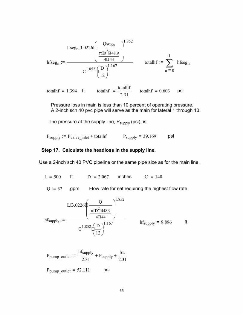
psi Ppump_outlet 52.111=

Ppump_outlethfsupply

2.31Psupply+

SL2.31

+:=

ft hfsupply 9.896=hfsupply

L 3.0226⋅Q

π D2⋅ 448.9⋅4 144⋅

1.852⋅

C1.852 D12

1.167⋅

:=

Flow rate for set requiring the highest flow rate.gpm Q 32:=

C 140:=inches D 2.067:=ft L 500=

Use a 2-inch sch 40 PVC pipeline or the same pipe size as for the main line.

Step 17. Calculate the headloss in the supply line.

psi Psupply 39.169=Psupply Pvalve_inlet totalhf+:=

The pressure at the supply line, Psupply (psi), is

Pressure loss in main is less than 10 percent of operating pressure.A 2-inch sch 40 pvc pipe will serve as the main for lateral 1 through 10.

psi totalhf 0.603=totalhftotalhf2.31

:=ft totalhf 1.394=

totalhf

0

1

n

hfsegn∑=

:=hfsegn

Lsegn 3.0226⋅Qsegn

π D2⋅ 448.9⋅4 144⋅

1.852⋅

C1.852 D12

1.167⋅

:=

65

K 19=

K

0

10

u

kvalueu∑=

:=

kvalueu

1.20.29.32.20.21.30.70.71.70.51.0

:=itemu

"solenoid valve""gate valve""strainer""check valve""union""tee""90 deg elbow""90 deg elbow""foot valve""entrance""exit"

:=

u 0 10..:=

Calculate the minor losses in the system.

fpsVsupply 3.059=VsupplyQ

π D2⋅ 448.9⋅4 144⋅

:=Velocity in supply line

Diameter of supply lineD 2.067=

psi hfsuc 0.072=hfsuchfsuc

2.31:=hfsuc

Lsuc 3.0226⋅Q

π Dsuc2⋅ 448.9⋅

4 144⋅

1.852⋅

C1.852 Dsuc

12

1.167⋅

:=

Diameter of suction pipe is one size largerthan the supply pipe line.

gpm Q 32:=inches Dsuc 2.469:=C 140:=ft Lsuc 20:=

Step 18. Calculate minor losses and headloss in suction pipe.

66

PLminor KVsupply

2

2 32.2⋅⋅

12.31

⋅:= PLminor 1.195= psi

Step 19. Calculate Total Dynamic Head

TDH PLminor hfsuc+( ) 2.31⋅ Ppump_outlet 2.31⋅+:=

TDH 123.303= ft TDHTDH2.31

:= TDH 53.378= psi

Need a pump that will pump 32 gpm at 124 ft of TDH.

67

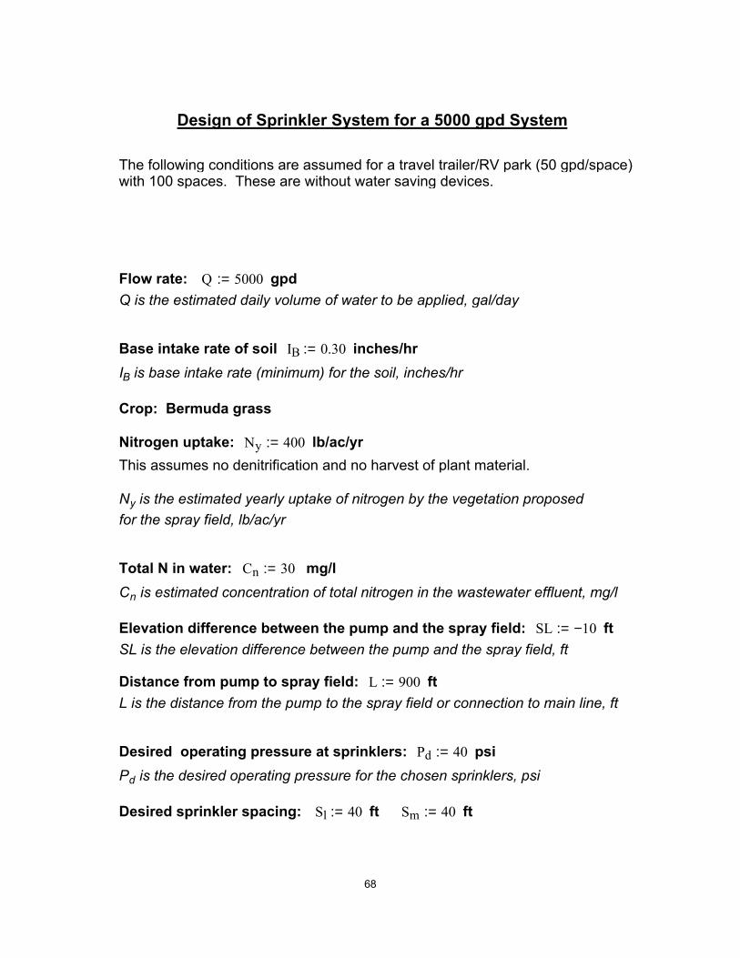
Design of Sprinkler System for a 5000 gpd System

The following conditions are assumed for a travel trailer/RV park (50 gpd/space)with 100 spaces. These are without water saving devices.

Flow rate: Q 5000:= gpdQ is the estimated daily volume of water to be applied, gal/day

Base intake rate of soil IB 0.30:= inches/hrIB is base intake rate (minimum) for the soil, inches/hr

Crop: Bermuda grass

Nitrogen uptake: Ny 400:= lb/ac/yr This assumes no denitrification and no harvest of plant material.

Ny is the estimated yearly uptake of nitrogen by the vegetation proposedfor the spray field, lb/ac/yr

Total N in water: Cn 30:= mg/lCn is estimated concentration of total nitrogen in the wastewater effluent, mg/l

Elevation difference between the pump and the spray field: SL 10−:= ftSL is the elevation difference between the pump and the spray field, ft

Distance from pump to spray field: L 900:= ftL is the distance from the pump to the spray field or connection to main line, ft

Desired operating pressure at sprinklers: Pd 40:= psiPd is the desired operating pressure for the chosen sprinklers, psi

Desired sprinkler spacing: Sl 40:= ft Sm 40:= ft

68

sl is the sprinkler spacing along the lateral, ftsm is the sprinkler spacing along the main, ft

Maximum surface storage on soil: SS 0.1:= inchesMaximum surface storage for the applied water, inches

Volume of storage tank: Vol 10000:= galVol is the volume of the storage tank between the alarm-on level and thepump-on level, gal

It is recommended that the Vol be 2 times the average daily volume of water, Q.

Step 1. Determine the amount of nitrogen being applied per year.

TnCn Q⋅ 8.34⋅ 365⋅

1000000:= Tn 456.615= lb/yr

Tn is the estimated pounds of total nitrogen being applied as a constituentof the wastewater effluent, lb/yr

Step 2. Determine the spray field area based on nitrogen application rate.

AreanTn

Ny43560⋅:= Arean 4.973 104×= ft2

Arean is the minimum area of the spray field assuming nitrogen is theland-limiting factor, ft2

Step 3. Determine the required area based on hydraulic loading rate.

Assume the daily average time of application is 30 minutes: TA 0.5:= hr

TA is the time of application of effluent on to the spray field, hr

The value for TA was assumed reasonalbe for an OSSF system. TA could beas long as 5 hours according to TNRCC regulations--285.33.

69

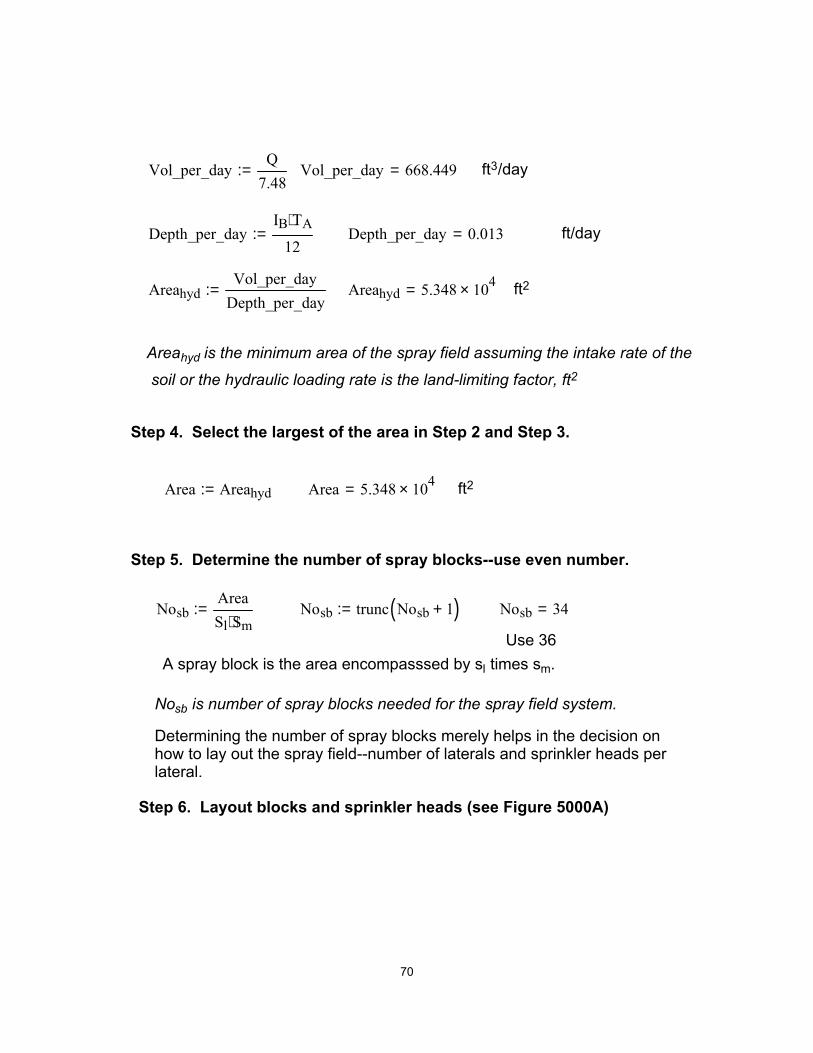
Step 6. Layout blocks and sprinkler heads (see Figure 5000A)

Determining the number of spray blocks merely helps in the decision onhow to lay out the spray field--number of laterals and sprinkler heads perlateral.

Nosb is number of spray blocks needed for the spray field system.

A spray block is the area encompasssed by sl times sm. Use 36

Nosb 34=Nosb trunc Nosb 1+( ):=NosbAreaSl Sm⋅

:=

Step 5. Determine the number of spray blocks--use even number.

ft2Area 5.348 104×=Area Areahyd:=

Step 4. Select the largest of the area in Step 2 and Step 3.

Areahyd is the minimum area of the spray field assuming the intake rate of the soil or the hydraulic loading rate is the land-limiting factor, ft2

ft2Areahyd 5.348 104×=AreahydVol_per_day

Depth_per_day:=

ft/dayDepth_per_day 0.013=Depth_per_dayIB TA⋅

12:=

ft3/dayVol_per_day 668.449=Vol_per_dayQ

7.48:=

70

Figure 5000A.- Preliminary Layout of Sprinkler System

Step 7. Determine maximum sprinkler discharge for a full circle sprinkler head based on the base intake rate of the soil, IB.

QsprIB Sl⋅ Sm⋅

96.3:= Qspr 4.984= gpm

Qspr is the discharge rate from a full-circle sprinkler head, gpm

Step 8. Determine maximum sprinkler discharge based on TA and SS.

QRIB TA⋅ SS+

TA:= QR 0.5= inches/hr

71

QR is the maximum application rate adjusted for surface storage and timeof application, inches/hr

QsprQR Sl⋅ Sm⋅

96.3:= Qspr 8.307= gpm

This sprinkler head discharge rate is based on allowing an adjustmentfor the surface storage and should be considered a maximum value.

Step 9. Select the sprinkler head--this may require a change in the operating pressure at the sprinkler head and the sprinkler spacing. This will require modifications to Steps 1-8.***********************************************************************************

This is where the design of a sprinkler system for an OSSF system differsfrom the design of a turf irrigation system. When designing a turf irrigationsystem, one is concerned with replenishing water in the soil profile and applying 1 to 2 inches of water per irrigation. One should be certain to make sure the application rate does not exceed the base intake rate of thesoil or there would be surface runoff.

However, for an OSSF system, the irrigation frequency is usually everyday and the depth of application will generally be less than 0.25 inches ofwater. The actual time of application will be small and the intake rate willalmost always be greater than the base intake rate because it takes timefor the intake rate to decrease to the base intake rate. Furthermore, one can take advantage of surface storage and apply water at a rate somewhat greater than the base intake rate.

With the above considerations in mind, an application rate could be very smallor large enough so that the maximum discharge from the sprinkler isachieved as calculated in Step 8. Thus for this design, one could selecta full circlesprinkler discharge rate from something near 2 gpm to 8.31 gpm andstill have an acceptable design.

After a review of various commercial sprinkler heads, a discharge rate of7.42 gpm was selected for a full-circle sprinkler head.

***********************************************************************************

72

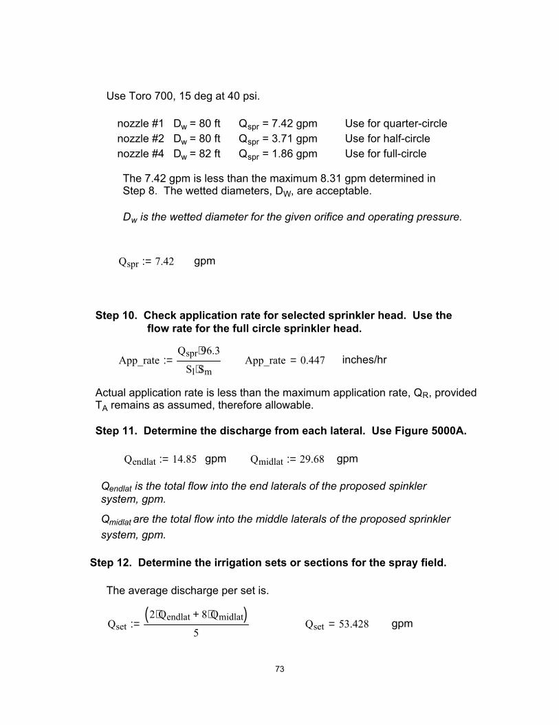
gpm Qset 53.428=Qset2 Qendlat⋅ 8 Qmidlat⋅+( )

5:=

The average discharge per set is.

Step 12. Determine the irrigation sets or sections for the spray field.

Qmidlat are the total flow into the middle laterals of the proposed sprinklersystem, gpm.

Qendlat is the total flow into the end laterals of the proposed spinkler system, gpm.

gpm Qmidlat 29.68:=gpm Qendlat 14.85:=

Step 11. Determine the discharge from each lateral. Use Figure 5000A.

Actual application rate is less than the maximum application rate, QR, provided TA remains as assumed, therefore allowable.

inches/hr App_rate 0.447=App_rateQspr 96.3⋅

Sl Sm⋅:=

Step 10. Check application rate for selected sprinkler head. Use the flow rate for the full circle sprinkler head.

gpm Qspr 7.42:=

Dw is the wetted diameter for the given orifice and operating pressure.

The 7.42 gpm is less than the maximum 8.31 gpm determined inStep 8. The wetted diameters, DW, are acceptable.

nozzle #1 Dw = 80 ft Qspr = 7.42 gpm Use for quarter-circlenozzle #2 Dw = 80 ft Qspr = 3.71 gpm Use for half-circlenozzle #4 Dw = 82 ft Qspr = 1.86 gpm Use for full-circle

Use Toro 700, 15 deg at 40 psi.

73

Each set of two adjacent lateralswill be a set. For this design, therewill be 5 sets.Number of sets Noset 5:=

Time to drain tank TdVolQset

:= Td 187.168= min

The above appears to be a reasonable time to drain a full tank. The timeneeded is less than the 5 hour window for application required by TNRCC-285.33

TsetTd

Noset:= Tset 37.434= min

The time of application, TA, is equal to the Tset.

It is recommended that the set time be 38 minutes for this system.

Tset 38:= min

TA Tset:=

Note: TA could have been changed to 0.63 hours and the area requiredcould have been reduced. The area required would be that need to assimulate the available nitrogen.

Step 13. Layout the pipe, sprinkler heads, control valves, and connection to the supply line (see Figure 5000B).

74

Figure 5000B.-Layout of sprinkler heads and control valves.

Step 14. Size the laterals. There must be less than 20 percent pressure loss along the lateral. Calculate the pressure loss starting with the last segment of pipe (attached to the last sprinkler head) and go to the control valve. Sum the headloss in each segment to obtain the total headloss in the lateral.

Roughness of pipe C 140:= Use sch 40 PVC pipe.

C is the Hazen-Williams pipe roughness factor for PVC pipe.

Laterals 1 and 10 are the same. .

Headloss for Laterals 1 and 10.n 0 3..:= D 1.049:= inches inside diameter

75

Qsegn

3.7111.1318.5525.97

:=Lsegn

40404040

:=Segmentn

1234

:=

inches inside diameterD 1.380:=n 0 3..:=

Headloss for Lateral 2-9 or the middle laterals.

psi totalhf 3.113=totalhftotalhf2.31

:=ft totalhf 7.19=

totalhf

0

3

n

hfsegn∑=

:=hfsegn

Lsegn 3.0226⋅Qsegn

π D2⋅ 448.9⋅4 144⋅

1.852⋅

C1.852 D12

1.167⋅

:=

Hazen-Williams formula for friction loss in a pipe.

Segment is the pipe segmentalong the lateral starting with the last sprinkler head.

Lseg is the length of each segmentin feet.

Qseg is the flow rate within eachsegment in gpm.

Qsegn

1.865.579.2812.99

:=Lsegn

40404040

:=Segmentn

1234

:=D is the inside diameter of the pipe in inches

76

Pn is the pressure at the first sprinkler head on the lateral, psi.

psi Pn 42.335=Pn Pf Po+:=

Po is the pressure at the sprinkler head at the distal end of lateral, psi.

Po 39.222=Po Pa 0.25 Pf⋅−:=

Pa Po 0.25 Pf⋅+=

Pa is the average operating pressure for the system, psi.

psi Pa 40:=

Pf is the headloss in the lateral, psi.

psiPf 3.113=Pf totalhf:=psi totalhf 3.113:=

Use the lateral with the greatest headloss. Use lateral 1.

Step 15. Determine pressure at the first and distal sprinkler heads. Determine pressure at outlet of control valve. Determine pressure at inlet to control valve.

Select 1 inch sch 40 PVC pipe for laterals one and ten and a 1-1/4-inch sch 40 PVC pipe for lateral 2-9 or the middle laterals. These pipe sizes meet the pressure loss criterion. The next smaller size pipes cause excess pressure losses.

psi totalhf 2.951=totalhftotalhf2.31

:=ft totalhf 6.818=

totalhf

0

3

n

hfsegn∑=

:=hfsegn

Lsegn 3.0226⋅Qsegn

π D2⋅ 448.9⋅4 144⋅

1.852⋅

C1.852 D12

1.167⋅

:=

77

Qsegn

0.0159.36

:=Lsegn

8580

:=Segmentn

12

:=

n 0 1..:=

inches inside diameterD 2.067:=

The supply line will discharge into the middle of the main line.

Step 16. Determine the size of the main line. The pressure loss in the main should be less than 10 percent of the average operating pressure of the sprinkler system.

psi Pvalve_inlet 48.241=Pvalve_inlet Pvalve_outlet PLvalve+:=

psi PLvalve 4.5:=

Pressure loss in valve, PLvalve, is found from manufacturers catalog.

psi Pvalve_outlet 43.741=Pvalve_outlet Pnhf25

2.31+:=

ft hf25 3.249=hf25

L25 3.0226⋅Q25

π D2⋅ 448.9⋅4 144⋅

1.852

⋅

C1.852 D12

1.167⋅

:=

gpm Q25 14.85:=ft L25 25:=inches inside diameterD 1.049:=

There is 25 feet of 1-inch pipe to control valve.

78

Ppump_outlethfsupply

2.31Psupply+

SL2.31

+:=

ft hfsupply 8.17=hfsupply

L 3.0226⋅Q

π D2⋅ 448.9⋅4 144⋅

1.852⋅

C1.852 D12

1.167⋅

:=

Flow rate for set requiring the highest flow rate.gpm Q 59.36:=

C 140:=inches D 3.068:=ft L 900=

Use a 3-inch sch 40 PVC pipeline.

Step 17. Calculate the headloss in the supply line.

psi Psupply 50.394=Psupply Pvalve_inlet totalhf+:=

The pressure at the supply line, Psupply (psi), is

Pressure loss in main is less than 10 percent of operating pressure.A 2-inch sch 40 PVC pipe will serve as the main for laterals 1 through 10.

psi totalhf 2.152=totalhftotalhf2.31

:=ft totalhf 4.972=

totalhf

0

1

n

hfsegn∑=

:=hfsegn

Lsegn 3.0226⋅Qsegn

π D2⋅ 448.9⋅4 144⋅

1.852⋅

C1.852 D12

1.167⋅

:=

79

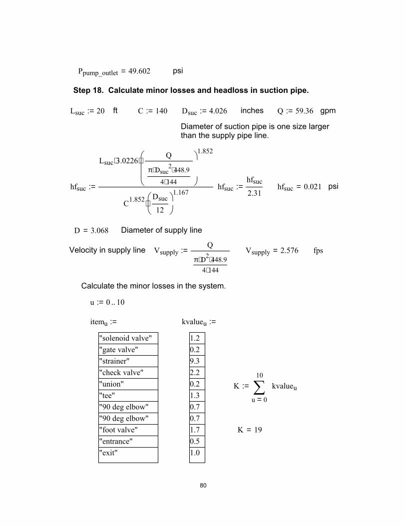
K 19=

K

0

10

u

kvalueu∑=

:=

kvalueu

1.20.29.32.20.21.30.70.71.70.51.0

:=itemu

"solenoid valve""gate valve""strainer""check valve""union""tee""90 deg elbow""90 deg elbow""foot valve""entrance""exit"

:=

u 0 10..:=

Calculate the minor losses in the system.

fpsVsupply 2.576=VsupplyQ

π D2⋅ 448.9⋅4 144⋅

:=Velocity in supply line

Diameter of supply lineD 3.068=

psi hfsuc 0.021=hfsuchfsuc

2.31:=hfsuc

Lsuc 3.0226⋅Q

π Dsuc2⋅ 448.9⋅

4 144⋅

1.852⋅

C1.852 Dsuc

12

1.167

⋅

:=

Diameter of suction pipe is one size largerthan the supply pipe line.

gpm Q 59.36:=inches Dsuc 4.026:=C 140:=ft Lsuc 20:=

Step 18. Calculate minor losses and headloss in suction pipe.

psi Ppump_outlet 49.602=

80

PLminor KVsupply

2

2 32.2⋅⋅

12.31

⋅:= PLminor 0.847= psi

Step 19. Calculate Total Dynamic Head

TDH PLminor hfsuc+( ) 2.31⋅ Ppump_outlet 2.31⋅+:=

TDH 116.585= ft TDHTDH2.31

:= TDH 50.47= psi

Need a pump that will pump 60 gpm at 117 ft of TDH.

81