Design, Construction and Commissioning of an Ortho-TOF ...
168
Design, Construction and Commissioning of an Ortho-TOF Mass Spectrometer for Investigations of Exotic Nuclei In Partial Fulfilment of the Requirements for the Degree of Doctor rer. nat. II. Physical Institute Justus-Liebig University Giessen Prepared by: Sergey Eliseev St. Petersburg, Russia Giessen, Germany 2004
Transcript of Design, Construction and Commissioning of an Ortho-TOF ...

Design, Construction and Commissioning of an Ortho-TOF Mass Spectrometer for Investigations
of Exotic Nuclei
In Partial Fulfilment of the Requirements for
the Degree of Doctor rer. nat.
II. Physical Institute
Justus-Liebig University Giessen
Prepared by:
Sergey Eliseev
St. Petersburg, Russia
Giessen, Germany
2004

Supervisor and Examiner: Prof. Dr. Geissel
Examiner: Prof. Dr. Metag
Examiner: Prof. Dr. Scheid

Contents Introduction ....................................................................................... 1 Chapter 1 Basic principles of modern time-of-flight mass
spectrometers..................................................................................... 5 1.1 Time-of-flight mass spectrometry.............................................................5
1.2 Radio-frequency quadrupole: ion trapping and cooling .........................13 1.2.1 Introduction.......................................................................................13
1.2.2 Theory of trapping and cooling.........................................................15
1.3 Ion sources ..............................................................................................19
1.3.1 Electrospray ion source ......................................................................19
1.3.2 Alkali and Alkali Earths ion source ...................................................21
1.3.3 Laser ionization ion source ................................................................24
Chapter 2 Experimental set-up .................................................... 25 2.1 Ion source................................................................................................25
2.2 Quadrupole..............................................................................................33
2.3 Einzel lens ...............................................................................................37
2.4 Time-of-flight analyzer ...........................................................................39
2.5 Detection system.....................................................................................42
2.6 Vacuum system .......................................................................................46
Chapter 3 Experimental results and discussion........................... 48 3.1 Investigation of cooling and trapping of the ions in the radio-frequency
quadrupole......................................................................................................48
3.1.1 Continuous mode ...............................................................................50
3.1.2 Bunch mode .......................................................................................56
3.2 Precision of mass determination ..............................................................68
3.3 Investigation of the efficiency and mass resolving power of the
Ortho-TOF mass spectrometer..................................................................74
3.3.1 Efficiency of the Ortho-TOF mass spectrometer ...............................74
3.3.2 Mass resolving power of the Ortho-TOF mass spectrometer ............77

Chapter 4 Theoretical investigation of the Ortho-TOF mass
spectrometer .................................................................................... 79
4.1 Mass resolving power ..............................................................................79
4.2 Efficiency .................................................................................................89
4.3 Further improvement of the Ortho-TOF mass spectrometer ...................89
Chapter 5 Experiment to characterize the SHIPTRAP gas cell ... 91 5.1 Experiment with the Er-laser source........................................................93
5.2 On-line experiment with 107Ag17+-beam provided from a tandem
accelerator ......................................................................................................95
5.2.1 Efficiency of the gas cell vs the intensity of the primary Ag-beam...95
5.2.2 Study of the chemical reactions in the gas cell ................................105
Chapter 6 On-line mass measurement of 107Ag ................. 110
Summary and outlook .............................................................. 113
Appendix 1: Principle of time-of-flight mass spectrometer..........I
Appendix 2: Einzel lens ................................................... VIII
Appendix 3: Space charge effect on an ion capacity of the
linear RFQ trap ............................................. XII
Appendix 4: Space charge of He-ions, created in the stopping
volume of the gas cell during the stopping of the
primary beam .......................................... XVIII
Appendix 5: Geometry and electrical settings of the Ortho-
TOF mass spectrometer ..............................XXVI
Acknowledgement ................................................... XXVIII
References.................................................................... XXX

Zusammenfassung Präzise Messungen atomarer Massen sind für viele wissenschaftliche Bereiche und
technische Anwendungen sehr wichtig. In der Kernphysik sind Massenmessungen
von kurzlebigen Nukliden fern ab vom Stabilitätstal von großer Bedeutung zum
besseren Verständnis der starken Wechselwirkung. In der nuklearen Astrophysik
haben Massen- und Lebensdauermessungen von Kernen entlang den Pfaden für die
Elementsynthese (bspw. r-, rp-Prozesse) in den Sternen eine zentrale Rolle, um den
Ursprung und die Zusammensetzung der sichtbaren Materie im Universum zu
verstehen. Für Biochemie und Medizin sind Massenmessungen in der
Strukturanalyse von komplexen Biomolekülen unverzichtbar. In der
Umweltwissenschaft werden Massenmessungen in der Spurenanalyse zur Indikation
von Giftstoffen verwendet.
Die präzisesten Massenmessungen an exotischen Nukliden sind entweder auf die
Bestimmung der Flugzeit (TOF), der Umlauffrequenz (RF) oder der
Zyklotronfrequenz (CF) eines Ions in den elektromagnetischen Feldern der
Massenspektrometer zurückzuführen.
Im Rahmen dieser Doktorarbeit wurde ein Flugzeitmassenspektrometer mit
orthogonaler Extraktion (Ortho-TOF MS) aufgebaut und in ersten Experimenten
erfolgreich eingesetzt. Ziele der Doktorarbeit waren, das Ortho-TOF MS
aufzubauen und ausführliche experimentelle Untersuchungen damit durchzuführen.
Dabei wurden die Ergebnisse mit Modellrechnugen verglichen, um die Funktionen
der verschiedenen Anteile der Spektrometerabschnitte zu verstehen. Der geplante
Einsatzbereich der Apparatur sind Massenmessungen und Spektroskopie an
exotischen Nukliden.
Das Ortho-TOF MS kann am Wienfilter SHIP für die Massenmessungen von
kurzlebigen Fusionsprodukten verwendet werden. Es kann komplementär zu den

SHIPTRAP Penning-Fallen benutzt werden, da diese aufgrund der Meßtechnik
keinen Zugang zu den kurzlebigsten superschweren Kernen haben. Der große
Massenbereich des Ortho-TOF-MS in einem Spektrum ermöglicht es darüber hinaus,
dieses als diagnostisches Gerät für die neue Generation von gasgefüllten Ion-Catcher
zu verwenden.
Andere Anwendungen, die in der Zukunft realisiert werden können, sind die
Untersuchung von chemischen Reaktionen der superschweren Kerne und die
massenaufgelöste Zerfallspektroskopie von Nukliden. Beispielsweise können die
doppeltmagischen 100Sn Isotope die mit hohen Produktionsquerschnitten in
Fusionsreaktionen gebildet werden, auch der Spektroskopie zugänglich gemacht
werden. Obwohl 100Sn Ionen am Fragmentseparator FRS entdeckt wurden, so ist die
Häufigkeit dieser Reaktionsprodukte an der Coulomb Barriere etwa um einen Faktor
1000 größer. Jedoch fehlt in diesem Energiebereich die selektive Separation. In
Zukunft wird eine solche Spektroskopie mit einem entsprechenden Massenfilter nach
dem Ortho-TOF Prinzip von unserer Gruppe angestrebt.
.
Die Entwicklung der Flugzeitspektrometer hat in unserem Institut schon eine längere
Tradition, jedoch waren die Anwendungsgebiete und damit die Anforderungen sehr
verschieden. So nützt es wenig, wenn eine hohe Massenauflösung erreicht wird, aber
die niedrige Akzeptanz und Transmission für die exotischen Kerne nicht adäquat
sind. Deshalb wurde zunächst eine ausführliche Untersuchung der Kühlungs- und
Speicherverhalten des RF-Quadrupoles durchgeführt. Der RF-Quadrupol hat eine
zentrale Rolle im Massenspektrometer, da er den Eingangsphasenraum präpariert
und festlegt.
Da das Ortho-TOF-MS ein universelles Gerät mit einem großen Massenbereich ist,
wurde es erfolgreich auch als Diagnosegerät für die Charakterisierung und
Optimierung der SHIPTRAP Gaszelle in Experimenten am Münchner Tandem –
Beschleuniger eingesetzt. Gerade für die Analyse der möglichen chemischen
Reaktionen in der Gaszelle sind solche Messungen essentiell.
Die maximale Effizienz des hier entwickelten Ortho-TOF-MS beträgt 1% und 3%
jeweils für den kontinuierlichen und den gepulsten Betrieb. Dieses Ergebnis
entspricht den theoretischen Abschätzungen und ist durchaus für Experimente am
SHIP geeignet.

Die erreichte maximale Präzision in einer Massenbestimmung mit den Pb-Isotopen
ist besser als 0,7 ppm, entsprechend etwa 100 keV. Theoretische Vorhersagen mit
mikroskopischen Modellen sind derzeit noch um Faktoren von 5 bis 10 schlechter
für exotische Kerne, so daß mit einer solchen Messgenauigkeit noch gute Beiträge
zum besseren Verständnis der Kernbindungsenergie geleistet werden können.
Die on-line Massenmessungen von stabilen 107Ag Projektilionen am Münchner
Tandem-Beschleuniger erreichten eine Präzision von 1.3 ppm, entsprechend 130
keV und sind somit etwas schlechter als die off-line Pb-Experimente. Jedoch sind
die Präzision und die absolute Genauigkeiten in Zukunft leicht mit den gewonnen
Erkenntnissen aus dieser Arbeit zu verbessern.


Introduction 1
Introduction Precise atomic mass measurements are very important in many disciplines of
science, e.g. in physics, biochemistry, medicine, archaeology and environmental
research. In nuclear physics, mass measurements of nuclides are essential for testing
nuclear mass models. From the knowledge of the mass of a nuclide the nuclear
binding energy can be derived. The mass measurements provide a better knowledge
of the strong interaction between the constituents in the nucleus. In nuclear
astrophysics, mass measurements of exotic nuclides are of great importance for our
understanding of the synthesis of the elements. In biochemistry and medicine, mass
measurement methods are helpful in a structural analysis of complex biomolecules.
Mass measurement techniques are widely used in the trace analysis of poisonous
substances in environmental research. Leak searchers and rest gas analysers are also
based on the principles of mass measurements.
The most precise methods of mass measurements, employed in nuclear physics, are
based either on the determination of the time of flight (TOF), the revolution
frequency (RF), or cyclotron frequency (CF) of the ion in mass spectrometers.
Nowadays, there are several scientific centers such as GSI, CERN, GANIL and ANL
employing these techniques. The RF-technique is realized at GSI in the
Experimental Storage Ring (ESR) [Fra87] (Schottky Mass Spectrometry SMS and
Isochronous Mass Spectrometry IMS) for ions produced in the in-flight FRagment
Separator (FRS) [Gei92]. At GANIL, the TOF-technique is employed at the Second
Separated-Sector Cyclotron (CSS2) and at the Spectrométre á Perte d’Energie du
Ganil (SPEG) [Bia89,Aug94]. The CF-technique is implemented in MISTRAL
[Lun01] and in Penning traps ISOLTRAP [Bol87, Her03] at ISOLDE (CERN). The
CF- technique is also used at SHIPTRAP [Dil01,Sik03] at GSI and at the Canadian
Penning Trap (CPT), coupled to the Argonne Tandem Linac Accelerating System
(ATLAS) at ANL [Sav01]. In the following diagram 1, the relative accuracy of mass
determination achieved by the above mentioned techniques and typical half-lives
reached by each method are presented.

Introduction 2
10-4 10-3 10-2 10-1 100 101 102 1031E-8
1E-7
1E-6
1E-5
1E-4Re
lativ
em
ass
accu
racy
Half-life (s)
SPEG
ESR-IMS
MISTRAL
ESR SMS
ISOLTRAP
CSS2
Diagram 1: Relative accuracy of mass determination achieved by the above mentioned techniques and
typical half-lives reached by each method
The IMS is expected to give access to very short-lived nuclides. The highest relative
mass accuracy for exotic nuclides (10-8) can be reached nowadays at ISOLTRAP.
Besides the techniques mentioned above there is a class of relatively small
(transportable) mass spectrometers based on the time-of-flight technique. Having the
accuracy of mass determination of exotic nuclei and access to short lived nuclei
comparable to the methods mentioned above, such mass spectrometers have a broad
mass band. Such versatile mass spectrometers (TOF MS) are intensively used in all
disciplines of science. The first report on a TOF MS is dated by the late 1940s by
Cameron and Eggers [Cam48]. Wiley and McLaren in 1955 [Wil55] built a linear
system with the mass resolving power of about 100. The low mass resolving power,
the lack of electronics that can operate in a nanosecond time range and the absence
of detectors suitable for such applications were the reasons for the very slow
development of TOF MS during the following two decades. The second birth of
time-of-flight mass spectrometry in the late 1980s was enabled by several break-

Introduction 3
throughs in the design of TOF MS, by the development of micro-channel plates, by
advances of fast timing electronics and by the invention of new ionization methods.
The realization of double stage ion reflectors by Mamyrin [Mam73] and grid-free
reflectors by Wollnik and Piyadasa [Wol99,Piy99] in TOF-MS increased the mass
resolving power up to a few thousands.The invention of the orthogonal extraction
method by Dodonov [Dod87,Dod91] allowed to increase the sensitivity of TOF-MS
without sacrificing mass resolving power.
For the registration of the ions in TOF-MS, micro-channel plate detectors are used
nowadays [Wiz79,Wur94,Wur96]. Such MCP detectors usually provide a peak
width of less than a nanosecond for a single ion.
For the data acquisition, the time-to-digital converter (TDC) is best suited due to its
high time resolution of the order of 100ps and its small dead time of the order of a
few nanoseconds.
The invention of matrix-assisted laser desorption ionization (MALDI) [Kar88] and
electrospray ionization (ESI) [Men88,Fen89] has caused a revolution in the mass
spectrometry for biological research.
In this thesis a mass spectrometer with orthogonal extraction based on the TOF-
technique is presented (Ortho-TOF MS). The goal in this thesis was to build and
commission the Ortho-TOF MS and to perform comprehensive theoretical and
experimental investigations of the Ortho-TOF MS for the application in nuclear
physics such as mass measurements of exotic nuclides.
The Ortho-TOF MS can be used at SHIPTRAP for mass measurements of short-
lived nuclides. It will be complementary to the SHIPTRAP Penning trap in the cases
when an access to the nuclides with the half-lives of a few 10 ms is required.
The broad mass range of the Ortho-TOF MS gives the valuable possibility to use
the Ortho-TOF MS as a diagnostic tool for characterization of the SHIPTRAP gas
cell and the Ion-Catcher gas cell at the FRS.
Other applications that may be attempted in the future are the investigation of
chemistry of super heavy nuclides (ion mobility, reaction rates) and the decay
spectroscopy of mass-identified nuclides. A good example is double magic 100Sn.
This thesis consists of six chapters. In Chapter 1 basic principles of time-of-flight
mass spectrometry are described. The experimental set-up (Ortho-TOF MS) is

Introduction 4
subject of Chapter 2. Chapter 3 presents a detailed experimental investigation of the
constituents of the Ortho-TOF MS that affect the mass resolving power, accuracy of
mass determination and efficiency. The achieved mass resolving power, accuracy of
mass determination and efficiency of the Ortho-TOF MS and their consistency with
the theoretical predictions are also the subject of Chapter 3. A comprehensive
theoretical investigation of the individual parts of the Ortho-TOF MS with respect to
such important parameters of the Ortho-TOF MS as the mass resolving power,
accuracy of mass determination and efficiency are presented in Chapter 4. Chapter 5
describes the on-line test of the SHIPTRAP gas cell with the Ortho-TOF MS. Mass
measurements that took place in Garching, are presented in Chapter 6.

Chapter 1 Basic principles of modern time-of-flight spectrometers 5
Chapter 1
Basic principles of modern time-of-flight
spectrometers
1.1 Time-of-flight mass spectrometry The basic principles of time-of-flight mass spectrometry can be understood from
Fig.(1-1). Ions with different mass-to-charge ratios (M/Q) have different flight-times
along the path l. After passing the path l they get spatially separated at the detector.
Kin
l E
M /Q1
M /Q2
Push plate
Detector
M /Q >1 M /Q2
E - electric field between push plate and detector
Kin- initial kinetic energy of the ions
l - distance between push plate and detector
Fig.(1-1): Basic principle of time-of-flight mass spectrometry. Ions with different mass-to-charge
ratios (M/Q) have different flight-times along the path l. After passing the path l they get spatially
separated at the detector.

Chapter 1 Basic principles of modern time-of-flight spectrometers 6
The time of flight of ions with mass M, electric charge Q and initial kinetic energy
Kin=0 along the path l can be expressed as follows (see Appendix 1):
E2l
QMt ×= (1_1)
It can be seen that a time-of-flight spectrometer separates ions with respect to their
mass-to-charge M/Q.
A schematic view of a linear time-of-flight mass spectrometer (linear TOF MS) is
shown in the Fig.(1-2) [Wil55,Wil00]. It consists of an ion source, an acceleration
region, a drift tube and a detector. The three regions are separated by grids. Ions are
stored or generated in the ion source. After the DC electric fields E1 and E2 are
applied between the push plate and the grid 1 (G1), and G1 and grid 2 (G2) (see
Fig.(1-2)), the ions start moving towards the detector with the energy K gained by
passing the regions with the electric fields E1 and E2. If the ions were at rest in the
ion source, there time of flight can be expressed as follows (Appendix 1):
(1_2)
tttt 321 ++=
E2l
2lQMt
11
11 = (1_3)
E2l)ElE2(l
2lQMt
112211
22
++= (1_4)
)ElE2(l
lQMt
2211
33
+= (1_5)
Here, t1 , t2 , t3 are the time-of-flight of the ion in the ion source, the acceleration
region and the field-free drift tube, respectively, l1 is the distance between the start
position of the ion and the first grid G1, E1 is the extracting field strength in the ion
source, E2 is the accelerating field strength , l2 and l3 are the lengths of the
acceleration region and the field-free drift tube.

Chapter 1 Basic principles of modern time-of-flight spectrometers 7
Push plate
detector
Ion_source
Accelerationregion
Field free drift tube
G1
G2
E1, 1, 1l t
E2, 2, 2l tE2,
3, 3 l t
Fig.(1-2): Schematic view of a simple linear time-of-flight mass spectrometer [Wil55,Wil00]. It
consists of an ion source, an ion acceleration region, a field free drift tube and a detector. Ions are
stored or generated in the ion source. After the DC electric fields E1 and E2 are applied between the
push plate and grid 1 (G1), and G1 and grid 2 (G2), the ions start moving towards the detector with
the kinetic energy K gained by passing the regions with the electric fields E1 and E2. The total flight-
time of the ions (t1+t2+t3) is a measure for M/Q.
The mass resolving power of a time-of-flight mass spectrometer Rm can be derived
from the time resolving power Rt as follows (see Eq.(1_1)):
M E2l
MQ1t ∆×=∆
21 (1_6)
2221 t
mR
tt
E2l
QM
tMMR =
∆=×
∆=
∆= (1_7)
Thus the mass resolving power Rm is given by
R
R tm 2= (1_8)

Chapter 1 Basic principles of modern time-of-flight spectrometers 8
Here the finite time interval corresponds to the full-width at half-maximum
height of the spectral peak (FWHM).
tΔ
It can be seen from Eq.(1_2)-Eq.(1-5) that the time-of-flight for the ions with the
same M/Q is the same only if the initial position of the ions in the ion source is the
same. In reality the ions in an ion source have both finite spatial and velocity
distributions in the z-direction. Fig.(1-3) illustrates four different possibilities:
Z
Push plate
(a) (b)
(d) z
z
∆Z Z0
(c)
Fig.(1-3): Fo
when there i
have a sprea
have differe
situation of
direction.
Case (a) s
velocity sp
and veloc
velocities
situation o
spread in t
A charact
compensat
v
ur d
s nei
d ∆z
nt in
ions i
how
read
ity s
in th
f ion
he z
erist
e (to
-v
Z
ifferent initial conditions of ions in the ion source. Case (a) shows the ideal case
ther a spatial nor a velocity and velocity spread in z-direction. In case (b) the ions
and zero velocity and zero velocity spread in the z-direction. In case (c) the ions
itial velocities in the z-direction but no a spatial spread. Case (d) is a realistic
n a ion source, where they have a spatial spread ∆z and a velocity spread in the z-
s the ideal case when there is neither a spatial nor a velocity and
in z-direction. In case (b) the ions have a spread ∆z and zero velocity
pread in the z-direction. In case (c) the ions have different initial
e z-direction but without a spatial spread. Case (d) is the common
s in a ion source, where ions have a spatial spread ∆z and a velocity
-direction .
ic feature of a time-of-flight mass spectrometer is its ability to
some extent) a finite spatial distribution of the ions (see Fig.(1-3)

Chapter 1 Basic principles of modern time-of-flight spectrometers 9
(b)). This feature is referred to as spatial focusing. The time-of-flight of an ion from
the start point z to the detector can be expanded:
.......zzt(z)
2!1z
zt(z)
1!1tt(z) 2
ZZ2
2
ZZ0 00+
∂∂
+∂∂
+= == ∆][∆][ (1_9)
where z0 is a reference start position of the ion in the ion source, ∆z = z – z0 .
Usually the condition of spatial focusing is formulated as follows:
0z
t(z)0ZZ =
∂∂
=][
. . . (1_10)
0zt(z)
0ZZn
n=
∂∂
=][
where n is the order of spatial focusing. It is clear that the higher an order of spatial
focusing is, the wider the spatial spread ∆z that can be compensated. It is easy to be
shown that for a linear time-of-flight mass spectrometer (Fig.(1-2)) only the second
order of spatial focusing can be fulfilled. The second order of spatial focusing can
be obtained by selecting the flight length l3 according to the condition [Wil55]:
)zl
kk1(1k2zl
0
2
00
23
003+
−= (1_11)
where 11
22100 El
ElEzk
+= and l1 ,l2, E1, E2 are defined in Eq.(1_2)-Eq.(1_5).
A linear time-of-flight mass spectrometer with 2 mm initial spatial spread of the
beam would have a resolving power ~6400 at a total flight distance of 20 cm. But the
presence of a velocity distribution of the ions in the z-direction (see Fig.(1-3) (c) and
(d)) leads to a substantial reduction of the mass resolving power of such a linear
time-of-flight mass spectrometer .
Let us consider two ions I1 and I2 with the same initial velocity ∆vz, however moving
in opposite directions, as shown in Fig.(1-3) (c). Ion I1 moves towards the push
plate and is decelerated by the extraction field E1 until it stops. It is then re-

Chapter 1 Basic principles of modern time-of-flight spectrometers 10
accelerated, returning to the starting position with its original speed but in the
reversed direction. Subsequently, the later motion of the ion I1 is identical to that of
the ion I2 but delayed by the turn-around time. This turn-around time, , can be
calculated as follows:
turntΔ
v 2Mt zturn
∆∆ =QE1
vz
vz vx
E1
M/Q (1_12)
This flight time error caused by the initial velocity spread can not be compensated by
any constant stationary electrical field.
For a linear time-of-flight mass spectrometer the time-of-flight distance and,
therefore, the time of flight t is coupled to the extraction field E1 and l1 (see Fig.(1-
2)), therefore, to the turn-around time . It limits the mass resolving power to a
few hundred for acceptable system parameters. Although several techniques were
used for the design of a linear time-of-flight mass spectrometer, the mass resolving
power could not be increased above ~ 5000 [Daw87,Gru94,Kev85]. Higher mass
resolving powers could only be achieved in reflection time-of-flight mass
spectrometers.
turntΔ
A reflection time-of-flight mass spectrometer (see Fig.(1-4)) consists of an ion
source, an accelerator, a field-free drift tube, a reflector and an ion detector. The
addition of the reflector decouples the time-of-flight distance from the extraction
field E1 and l1. It allows to increase the time of flight t and, therefore, the mass
resolving power, independently on E1 and l1 . The idea of a reflection time-of-flight
mass spectrometer is that the variations of the time-of-flight due to different ion
energies are compensated by corresponding variations of their time-of-flight in the
reflector, i.e. ions with higher energies will penetrate more deeply into the reflector
and therefore travel on a longer flight path inside the reflector.
For an ion which was at rest before acceleration, the total time-of-flight in a
reflection time-of-flight mass spectrometer as shown in Fig.(1-4) can be expressed
as follows (see Appendix 1):

Chapter 1 Basic principles of modern time-of-flight spectrometers 11
l
reflector
detector
Push plate
Z0zE l1 1
E l2 2
E l3 3
E l4 4
Fig.(1-4): Schematic view of a reflection time-of-flight mass spectrometer. It consists of an ion
source, an ion accelerator, a field-free drift tube, a reflector and an ion detector. The addition of the
reflector decouples the time-of-flight distance from the extraction field E1 and l1. It allows to increase

Chapter 1 Basic principles of modern time-of-flight spectrometers 12
the time of flight t and, therefore, the mass resolving power, independently on E1 and l1
.
EEl
EEl
z)EE
EE
2(
EEl
z
l
EElz)
EE2
EE(z)
EE(1
QE2Mt(z)
1
33
1
22
4
1
3
1
1
22
1
22
3
1
2
1
2
1
1
⎥⎥⎦
⎤++−+
+
+
++−+⎢⎣
⎡−=
(1_13)
where z is the start position of the ion, QM is the mass-to-charge ratio of the ion,
E1 is the extracting field strength, E2 is the accelerating field strength, E3 is the field
strength of the first stage of the reflector, E4 is the field strength of the second stage
of the reflector, l1, l2 , l, l3 , l4 are the length of the ion source, the ion accelerator, the
drift tube, the first stage of the reflector and the second part of the reflector.
If the average ion start position z0 in Fig.(1-4) is taken as the reference for the start
position of the ion, Eq.(1_13) can also be written as:
.......zzt(z)
2!1z
zt(z)
1!1tt(z) 2
ZZ2
2
ZZ0 00+
∂∂
+∂∂
+= == ∆][∆][ (1_14)
Postulating the condition for second order focusing
0z(z)t
0ZZ =∂∂
=][
0zt(z)
0ZZ2
2=
∂∂
=][ (1_15)
one can find the relations between E1 , E2 , E3 , E4 and l1, l2 , l, l3 , l4 . (See
Appendix 1).
Chapter 1 Basic principles of modern time-of-flight spectrometers 13
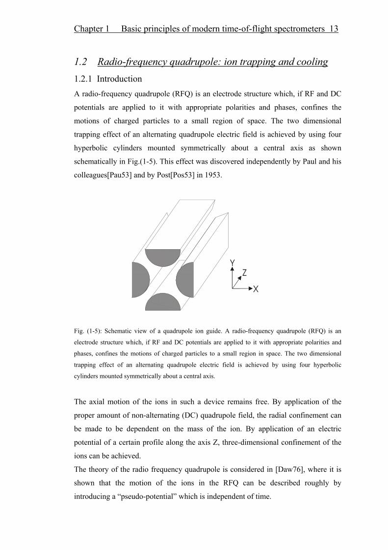
1.2 Radio-frequency quadrupole: ion trapping and cooling 1.2.1 Introduction A radio-frequency quadrupole (RFQ) is an electrode structure which, if RF and DC
potentials are applied to it with appropriate polarities and phases, confines the
motions of charged particles to a small region of space. The two dimensional
trapping effect of an alternating quadrupole electric field is achieved by using four
hyperbolic cylinders mounted symmetrically about a central axis as shown
schematically in Fig.(1-5). This effect was discovered independently by Paul and his
colleagues[Pau53] and by Post[Pos53] in 1953.
YZ
X
Fig. (1-5): Schematic view of a quadrupole ion guide. A radio-frequency quadrupole (RFQ) is an
electrode structure which, if RF and DC potentials are applied to it with appropriate polarities and
phases, confines the motions of charged particles to a small region in space. The two dimensional
trapping effect of an alternating quadrupole electric field is achieved by using four hyperbolic
cylinders mounted symmetrically about a central axis.
The axial motion of the ions in such a device remains free. By application of the
proper amount of non-alternating (DC) quadrupole field, the radial confinement can
be made to be dependent on the mass of the ion. By application of an electric
potential of a certain profile along the axis Z, three-dimensional confinement of the
ions can be achieved.
The theory of the radio frequency quadrupole is considered in [Daw76], where it is
shown that the motion of the ions in the RFQ can be described roughly by
introducing a “pseudo-potential” which is independent of time.
Chapter 1 Basic principles of modern time-of-flight spectrometers 14
Unlike the real potential, the pseudo-potential can have a minimum at the same
position in space for both the negative and the positive ions, thus trapping both types
at once.
Here, as an introduction, a qualitative description of the ion motion in the RFQ will
be given.
Let us consider the total effect of an alternating electric field over one cycle. Over
exactly one-half of the cycle the ion is pushed toward the stronger electric field
region (away from trap center) while over the other half it is pushed toward the
weaker region (toward trap center). However, the push toward the stronger field,
which occurs while the ion is in the weaker field, will be weaker than the push
toward the weaker field region. Hence the ion will progress toward the weaker field.
Since the weakest field of a quadrupole is at its center, where it is zero, the ions will
be driven to collect about the axis.
It was thought long time that such RF-devices can function only at high vacuum
( ). In 1992 the collisional focusing effect of ions in RFQ at
increased pressure was discovered [Dou92]. The ions, moving in an alternating
quadrupole field and undergoing collisions with residual gas, are focused on the axis
of the quadrupole. If the ions originally have large spatial and energy distributions
(a large phase space), then while moving in the RFQ their phase space becomes
smaller and their energy distribution approaches a Maxwell-Bolzman distribution
related to the corresponding temperature of the residual gas (thermalization of ions).
mbar1010 74 −− −
First the effect of “thermalization of ions” in an RFQ was used for an investigation
of low temperature ion-molecular reactions [Die92]. On the other hand, such a
method of reducing the phase space of an ion beam has proved to be very useful and
promising in mass-spectrometry, because the phase space of ions is directly related
to the resolving power and a sensitivity of a mass-spectrometer. In the work
[Moo88] the ions from an accelerator after collecting and cooling in a three-
dimensional quadrupole trap were injected into a time-of-flight mass spectrometer
for mass analysis.
For the first time in the works [Kru95,Kru98] such an RFQ with buffer gas was used
with an electrospray ion source. Recently [Lob98] it was coupled to a MALDI ion
source. In the work [Koz99] such a device was used as a molecular-ion reactor
(MIR) for the investigation of different fragmentation reactions.

Chapter 1 Basic principles of modern time-of-flight spectrometers 15
1.2.2 Theory of trapping and cooling A very detailed survey of the theory and properties of different multipole ion-
transport systems is presented in the works [Die92,Daw76].
In this work only RF-only mode of a radio-frequency quadrupole is considered.
The movement of ions in RF-multipoles with residual gas was analyzed with help of
different analytical and numerical methods [Kru98, Die92, To197, Mar89, To097].
While the method of numerical modeling has many advantages such as, for instance,
precise calculations of ion trajectories in an RFQ, it is not illustrative and it does not
give a possibility to make conclusions about behavior of the system with respect to
some basic parameters of an RFQ. Thus, in spite of many restrictions, approximate
analytical methods of describing such system have been proven to be very useful and
promising. In the work [Daw76] applying a method of the theory perturbation theory
in its most general form an expression for so-called pseudo-potential in case of a
movement of ions in vacuum was derived.
r rM
VQ(r)U 2
2
2rf
eff 40Ω
= (1_16)
where is a pseudo-potential, independent of time, and M are the electrical
charge and mass of the ion respectively, is the amplitude of harmonically
oscillating electric potential, r is the average coordinate of the ion, Ω is the angular
frequency of electric potential.
(r)Ueff Q
rfV
The method implemented in the work [Tol97] has been proven to be very fruitful. In
this approach the collisions of the ion with the molecules of the residual gas is
considered( viscous force approach [Mar89] ).

Chapter 1 Basic principles of modern time-of-flight spectrometers 16
RFU
R
Fig.(1-6): In technical realization a typical RF
which potentials in RF-only mode are applied i
Undergoing a collision with a residual
the work [Tal62] it was shown that the
and the residual gas molecule produce
after the collision their flight progresses
Provided the residual gas molecule is a
the velocity equal to the mean velocity
heavy ions, 1mM
ff ), one can write a
moving in gas [Koz99]:
QE∆t = M∆v + mvω∆t
where E is the electrical field strengt
electrical charge of the ion, m is the m
mean frequency of collisions of the ion
unit, k is a gas-kinetic constant of
molecules. For ∆t→0 Eq.(1_17) can be
MQE
τv
dtvd
=+
0
-only quadrupole consist of four cylindrical rods, to
n pairs.
gas molecule the ion changes its velocity. In
ion with the kinetic energy less than a few eV
a compound during the collision, therefore
isotropically.
t rest before a collision with the ion and gains
of the ion after a collision (which is valid for
n equation of momentum balance for the ion
(1_17)
h, M, v, Q is the mass, mean velocity and
ass of the residual gas molecule, ω=kn is the
with molecules of the residual gas per time
collisions, and n is the density of the gas
transformed into the following form:
(1_18)

Chapter 1 Basic principles of modern time-of-flight spectrometers 17
where ωm
Mτ = is the characteristic time of relaxation of the ion velocity.
In the approximation when ω depends weakly on the ion velocity the so-called
mobility ratio is fulfilled:
EMQτEv == κ (1_19)
where MQτ
=κ is the ion mobility.
Let us consider the movement of the ion in an RF-only quadrupole with residual gas.
In a practical technical realization a typical RF-only quadrupole consist of four
cylindrical rods, to which potentials in RF-only mode are applied in pairs (see
Fig.(1-6)). In such a geometry the electrical field between the rods can be described
by two independent components [Daw76] (This holds for ideal hyperbolic rods and
only approximately for cylindrical rods):
t cosVr2yE
t cosVr2xE
rf2y
rf2x
Ω−=
Ω= (1_20)
where Ω is the angular frequency and is the amplitude of the radio-frequency
voltage applied to a pair of the rods, r
rfV
0 is the distance between the axis of the
quadrupole and the rod. In this case Eq.(1_18) can be separated into two independent
equations for the x – and y- coordinates:
t cos
MQV
r2y
dtdy
τ1
dtyd
t cosM
QV
r2x
dtdx
τ1
dtxd
rf2
02
2
rf2
02
2
Ω−=+
Ω=+
(1_21)
These equations are identical to the Mathieu equation [Daw76] for ion movement in
vacuum except for the second term in Eq.(1_21) that is called a viscous term.

Chapter 1 Basic principles of modern time-of-flight spectrometers 18
A solution of these equations [Tol97] allows to obtain formulae for the pseudo-
potential and a mean radius squared of the ion beam in presence of residual gas in
the RF-quadrupole:
2τ21
2τ2
4r2)QM(
2r2VU
0
rfquadeff
Ω+
Ω
Ω= (1_22)
2τ2
2τ21Tk2V
4r2
2Q
M2R 0brf
00
Ω
Ω+Ω= (1_23)
The stability of ion movement in a RF-quadrupole in case of vacuum is characterized
by the Mathieu-parameter q [Daw76],
Mr
4QVq
220
rf
Ω= (1_24)
In case of vacuum ( 0)τ(1 →Ω ), when q 0.906, the movement of ions in an RF-
quadrupole becomes unstable; Mean velocity and oscillation amplitude of ions
increase exponentially with time. Since such a situation is realized at
f
220
rf0
0.906r
4QVMM
Ω== , this mass is called light-ion-mass cut-off.
With a growth of the viscous friction, the relaxation time τ becomes smaller, which
according to Eq.(1_22) leads to a reduced pseudo-potential and an increased mean
radius of the ion beam.
In a pseudo-potential, focusing ions on the axis of a quadrupole, the average
movement of the ion due to collisions with residual gas molecules is a periodic or
non-periodic relaxation depending on friction magnitude [Koz99]. The ions are
focused on the axis of the quadrupole, the kinetic energy spread of the ions in
stationary condition is doubled kinetic energy spread of the residual gas. The
equilibrium distribution of ions over the radius in an RF-only quadrupole is given in
[Koz99]:

Chapter 1 Basic principles of modern time-of-flight spectrometers 19
))rr)(
M2m((1
nn(r)
m2M
2
0
0
+
= (1_25)
where n(r) and n0 are the densities of the ions at distance r off the axis and on the
axis of the RFQ respectively, r0 is the radius of the RFQ, all other quantities are
defined in Eq.(1_17).
1.3 Ion sources In this subchapter three different types of ion sources are described. Each ion source
is able to produce only certain ion species. Thus, the type of an ion source should be
chosen according to the ion species required for the particular experiment or
application.
1.3.1. Electrospray ion source The production of ions by evaporation of charged droplets obtained through spraying
or bubbling, has been known for about a century, but it was only fairly recently
discovered that these ions may hold more than one charge[Gie84]. A model for ion
formation in ESI (electrospray ion source), containing the commonly accepted
themes, is described below [Fen93].

Chapter 1 Basic principles of modern time-of-flight spectrometers 20
++
+
Fc
Fs
High Voltage
Capillary needlewith analyte solution
Drying gas
Fig.(1-7): A basic principle of an electrostray ion source. Large charged droplets are produced by
‘pneumatic nebulization’; i.e. the forcing of the analyte solution through a needle, where a high
voltage (usually about 3000 V) is applied. The polarity of the applied voltage depends on the sign of
the ion charge. Due to the voltage the emerging solution is dispersed into a very fine spray of charged
droplets all at the same polarity. The solvent evaporates away, shrinking the droplet size and
increasing the charge concentration at the droplet’s surface. Eventually, at the Rayleigh limit [Ray82],
Coulombic repulsion overcomes the droplet’s surface tension and the droplet explodes.
Large charged droplets are produced by ‘pneumatic nebulization’; i.e. the forcing of
the analyte solution through a needle (see Fig.(1-7)), at the end of which is applied a
high voltage (usually about 3000 V). The polarity of the applied voltage depends on
the sign of the ion charge. Due to the voltage the emerging solution is dispersed into
a very fine spray of charged droplets all at the same polarity. The solvent evaporates
away, shrinking the droplet size and increasing the charge concentration at the
droplet’s surface. Eventually, at the Rayleigh limit [Ray82], Coulombic repulsion
overcomes the droplet’s surface tension and the droplet explodes.
The Rayleigh limit can be expressed as follows:
)R( 8Q 21
30γεπ= (1_26)

Chapter 1 Basic principles of modern time-of-flight spectrometers 21
where Q is the droplet charge, R is the droplet radius, is the permittivity of
vacuum, and is the surface tension of the solvent.
0ε
γ
This ‘Coulombic explosion’ forms a series of smaller, lower charged droplets. The
process of shrinking followed by explosion is repeated until individually charged
‘naked’ analyte ions are formed. The charges are statistically distributed among the
analyte’s available charge sites, leading to the possible formation of multiply
charged ions under the correct conditions. Increasing the rate of solvent evaporation,
by introducing a drying gas flow counter current to the sprayed ions (see Fig.(1-7))
increases the extent of multiple-charging. Decreasing the capillary diameter and
lowering the analyte solution flow rate i.e. in nanospray ionization, will create ions
with higher QM ratios (i.e. it is softer ionization technique) than those produced by
‘conventional’ ESI and are of much more use in the field of bioanalysis.
1.3.2 Alkali and Alkali Earths ion source Heating a sample substance to a high temperature on a surface of a metal (a filament)
by passing an electric current through the filament in vacuum causes positive ions
and neutral species to desorb from its surface. Because of the high temperature
involved, only certain elements are useful for construction of the filament. Typically
platinum, rhenium, tungsten and tantalum are used because they are metallic and can
be heated to temperatures of about 1000 to over 2000 C without melting. A further
important criterion for the filaments is that they should not readily react chemically
with surrounding gas or with any sample placed on them. Since hot filaments are
used in a high vacuum so as to facilitate evaporation and the manipulation of the
emitted ions and neutrals, interaction of the filaments with air or background vapors
is automatically reduced to a low level.
0
Samples examined by surface emission are almost always inorganic species because,
at the high temperatures involved, any organic material is seriously degraded
(thermolysed) and will react with the filaments. At temperatures of 1000 to 2000 0 C,
most inorganic substances yield positive ions without reacting with the typical
filament elements listed below.
To obtain positive ions from a sample, it must come into contact with the filament.
This may be done by directing a gas or vapor over the hot filament but, more
usually, the sample is placed directly onto a cold filament, which is then inserted into
the instrument and heated. A consequence of the high temperatures is that much of

Chapter 1 Basic principles of modern time-of-flight spectrometers 22
the sample is simply evaporated without producing isolated positive ions. There is a
‘competition’ between formation of positive ions and the evaporation of neutral
particles. Since only charged particles are of interest for TOF mass spectrometry, it
is important for maximum sensitivity that the ratio of positive ions to neutrals should
be as large as possible. Eq.(1_27) governing this ratio is given below[Val00]:
Aenn I)/kT(
0−
+
= φ (1_27)
where 0nn+ is the ratio of the number of positive ions to the number of neutrals
evaporated at the same time from a hot surface at temperature T, k is the Boltzman
constant and A is another constant (often taken to be 0.5), the expression ϕ -I is the
difference between the ionization energy (I; sometimes known as the ionization
potential) of the element or neutral, from which the ions are formed and the work
function (ϕ or sometimes W) of the metal from which the filament is made. The
ionization energy and the work function control the energy needed to remove an
electron from a neutral atom of the sample and the material from which the filament
is constructed. The difference between I andϕ governs the ease with which positive
ions can be formed from sample molecules lying on the filament. Some typical
values for ionization energies and work functions are give in Tables 1 and 2. By
inserting a value for k and adjusting the Eq.(1_27) to common units (eV) and putting
A = 0.5, the simpler Eq.(1_28) is obtained.
0.5enn I)/T(10*11,6
0
3 −+
= φ (1_28)
where T is in Kelvin degree, φ and I are in eV.
Examination of Eq.(1_28) reveals that, for ϕ >I, the expression (ϕ -I) is positive,
hence the greater the temperature, the smaller the proportion of positive ions to
neutrals. For example, with a sample of caesium (ionization energy, 3.89 eV) on a
tungsten filament (work function, 4.5 eV) at 1000 K, the ratio of 0nn+ =591. Thus,
for every caesium atom vaporized, some 600 atoms of Caesium-ions are produced.
At 2000 K, the ratio 0nn+ becomes 17 and only about 20 ions of caesium are
evaporated for every Cs-atom. Clearly, the lower the ionization energy with respect
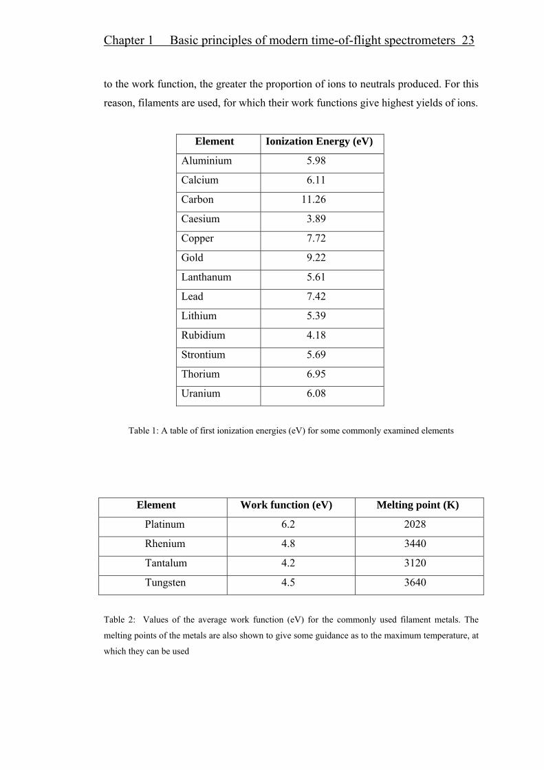
Chapter 1 Basic principles of modern time-of-flight spectrometers 23
to the work function, the greater the proportion of ions to neutrals produced. For this
reason, filaments are used, for which their work functions give highest yields of ions.
Element Ionization Energy (eV)
Aluminium 5.98
Calcium 6.11
Carbon 11.26
Caesium 3.89
Copper 7.72
Gold 9.22
Lanthanum 5.61
Lead 7.42
Lithium 5.39
Rubidium 4.18
Strontium 5.69
Thorium 6.95
Uranium 6.08
Table 1: A table of first ionization energies (eV) for some commonly examined elements
Element Work function (eV) Melting point (K)
Platinum 6.2 2028
Rhenium 4.8 3440
Tantalum 4.2 3120
Tungsten 4.5 3640
Table 2: Values of the average work function (eV) for the commonly used filament metals. The
melting points of the metals are also shown to give some guidance as to the maximum temperature, at
which they can be used

Chapter 1 Basic principles of modern time-of-flight spectrometers 24
1.3.3 Laser ionization ion source The laser ionization of the elements placed in the target of the ion source can occur
resonantly and non-resonantly. In order that resonant ionization can take place the
nuclide that is to be ionized must have an electromagnetic transition between two
electron shells, the energy of which should coincide with the frequency of the laser
radiation (Elaser = hν). Thus, resonant ionization is selective and applicable only to a
few species. In the case of non-resonant ionization the laser beam hitting the target
transfers the momentum to the target and, therefore, kinetic energy. As the result, the
target gets heated and ionization of the target material occurs (laser ablation).

Chapter 2 Experimental set-up 25
Chapter 2
Experimental set-up
The Ortho-TOF mass spectrometer
The design of the Ortho-TOF MS is based on a system developed by A. Dodonov et
al. [Dod87,Dod94]. A detailed scheme of the Ortho-TOF MS is shown in Fig.(2-1).
Ions produced in the ion source (1) enter a gas filled RF-only quadrupole (2) where
they are cooled. After extraction out of the RF-only quadrupole, the cooled ions pass
an einzel lens (7) and enter the modulator (10). In the modulator the ions are pushed
by a pulsed electric field in the direction perpendicular to the initial beam direction
and are accelerated in the accelerator (13). The time-of-flight of the ions from the
modulator to the MCP-detector (21) is a measure for mass-to-charge ratio of the
ions. Fig.(2-2) is a photo of the Ortho- TOF MS and electronics dedicated to it.
2.1 Ion source Different ion sources were used in this work. The choice of the type of the ion source
depended on the task that the author was going to carry out.
As it was already mentioned in chapter 1, three different types of ion sources can be
used with the Ortho-TOF MS.
Schematic views of the ion sources are presented in Fig.(2-3(a,b,c)).

Chapter 2 Experimental set-up 26
10E-5Torrpump 270L/s
10E-7Torrpump 400L/s
RFQ DCQ
to CFD/TDC
2 34 5 6
78
9
1011
12 1314
15
16
17
18
19
20
21
22
1. Ion Source2. RF only quadrupole3. skimmer24.DC-quadrupole5.output orifice6.moveable slit17.Einzel lens8.moveable slit2 9.field screen10.modulator11.grid112.grid213.accelerator14.grid315.field free flight tube16.grid417.first reflector stage18.grid519.backplate20.grid621.MCP-detector22.coupling capacity23.Faraday cup24.Topflange25.Interface flange
23
25 24
Ion SourceIons
50cm
Fig.(2-1): Schematic view of the Ortho-TOF MS. Ions produced in the ion source (1) enter the gas
filled RF-only quadrupole (2) where they get cooled. After extraction from the RF only quadrupole
the cooled ions passing the einzel lens (7) enter the modulator (10). In the modulator the ions get
repelled in the direction perpendicular to the initial beam direction and get accelerated in the
accelerator (13). The time-of-flight of the ions from the modulator to the MCP-detector (21) is a
measure for M/Q ratio of the ions.

Chapter 2 Experimental set-up 27
Fig.(2-2) : A photo of the Ortho-TOF MS and electronics dedicated to it.
teflon ring
pressed gas
pump0-0.4 l/minµ
syringemethanol
gas curtain
nozzle
Teflon capillary
1000V
200V
Φ0.15mm
10--30mm
3-5KV
encounter gas flow
A
metal capillaryfused silicon needlei.d. 50 mφ µ
700-1000V
Gas curtain
Nozzel 0.15φ mm
Focus electrode3.5φ mm
Unozzle
Us1
MIR
Fig.(2-3(a)): Schematic view of the electrospray ion source. It consists of a syringe pump with an
infusion syringe, a teflon capillary that contains the sample, a stainless steel capillary, a connecting
teflon capillary, a fused silicon spray needle, and a gas curtain. The sample (about 20 µl) is stored in
the 20 cm long teflon capillary of 400 µm inner diameter. The sample is injected at a 0.1 ~ 0.4 µl/min
flow rate controlled by the syringe pump (KD Scientific 88, kdScientific Inc., USA), whose syringe is
filled with methanol in advance.

Chapter 2 Experimental set-up 28
Iheating
Vions Vcurrent Vfocusing
Cs - fillement
Ceramic spacers
Current electrodePush electrode
Fig.(2-3(b)): Schematic view of the Cs ion source. It consists of a filament and an electrode structure.
The filament is a aluminosilicate sponge which contains Cs. The remarkable feature of such a sponge
structure is its large effective surface. The larger the effective surface of the source is the higher the
emitted Cs-Ion current of such a source is.
Ceramic insulating Upper focusing electrobe
Lower focusing electrobe
Laser beam
Entrancehole
Exit hole
Sample
Central electrode
Vupper
Vcentral
Vlower
Ions
Ion beam
Fig.(2-3(c)): Schematic view of the Laser ion source. It consists of three electrodes: a central
electrode, an upper electrode and a lower electrode. The central electrode serves as a holder for the
target. Two holes are made in the upper and the lower electrodes and serve for guiding the laser beam
from the laser onto the target. The target is placed on the central electrode. The central electrode is
moveable, so the position of the target can be adjusted to the laser beam.

Chapter 2 Experimental set-up 29
1. Electrospray ion source
The electrospray ion source (see Fig.(2-3(a))) consists of a syringe pump with an
infusion syringe, a teflon capillary that contains the sample, a stainless steel
capillary, a connecting teflon capillary, a fused silicon spray needle, and a gas
curtain. The sample (about 20µl) is stored in the 20 cm long teflon capillary of 400
µm inner diameter. The sample is injected at a flow rate of 0.1 ~ 0.4 µl/min, which is
controlled by the syringe pump (KD Scientific 88, kdScientific Inc., USA), whose
syringe is filled with methanol in advance. A fully filled sample capillary can sustain
the spray for about half an hour. A voltage of about +3500 V (for positive ions) is
applied to the sample through the stainless steel capillary, which is connected to the
spray needle by a short teflon capillary. The spray needle typically is of 100 µm
outer and 50 µm inner diameter and located 1 ~ 3 cm from a counter electrode (gas
curtain, in Fig.(2-3(a))). Supposing that the counter electrode is large and planar, the
electrical field at the capillary tip can be calculated using the approximate
relationship [Pfe68]:
)
r8dln(r
4VE
cc
cc = (2_1)
where Vc is the voltage drop between the needle and the gas curtain electrode, rc is
the outer radius of the tip of the capillary , and d is the distance from the capillary tip
to the counter electrode. According to Eq.(2_1), Ec is proportional to Vc, inversely
proportional to rc, and decreases slowly with the electrode separation d due to the
logarithmic dependence. Because it is easy to reduce the value of rc in order to obtain
a higher electrical field E in the region at the tip of the spray needle, the needle tip
should be prepared as a small cone.
The electrospray ion source is operated at a pressure of one atmosphere. The ions
extracted out of the syringe move through a dry nitrogen counter flow and pass
through a nozzle into the first gas-filled RF-quadrupole, i.e. molecule-ion reactor
(MIR). As a part of electrospray ion source the MIR serves as (1) an interface
between the 1 atmosphere and the second RF-only quadrupole in which a typical
pressure is 5*10-3 mbar, (2) a device that reduces the emittance of the beam coming
into the MIR to the proper value needed in order to be accepted by the second RF-

Chapter 2 Experimental set-up 30
only quadrupole, and (3) A device that removes adducts or moreover molecule ion
decomposition by varying the strength of the electrical field applied along the MIR.
From the principle of operation of electrospray it is seen that the samples that one
wants to investigate must be prepared in liquid form. This technique is widely used
in biochemistry and medicine in order to deliver organic samples to a TOF MS.
Usually such organic samples (gramicidin, insulin-β chain, fibrinopeptide-β ) are
dissolved in the methanol or acetonitrile. In many cases 2% acetic acid is added for
better spray condition. In order to generate light ions, salts like NaCl, KCl, CsI, PbI2
can be used. The typical concentration of the samples is about 10-5 M.
2. Cs-ion source
The Cs-ion source, built by the author (see Fig.(2-3(b))), consists of a filament and
an electrode structure. The filament is a aluminosilicate sponge which contains Cs.
The remarkable feature of such a sponge structure is its large effective surface. As
was described in the previous chapter the larger the effective surface of the source is
the higher the emitted Cs-ion current of such a source. In this work a commercial
aluminosilicate Cs-filament (TB-118, HeatWave Labs Inc, USA) was used. The push
electrode serves to convey kinetic energy to the ions. The current electrode is used
for measuring the emission current of the filament. It can also be used as a shutter
electrode if one wants to bunch the ion current. The focusing electrode is used for
varying the focusing condition of the ion source. The measured dependence of the
ion source current on the heating current of the filament is presented in Fig.(2-4).
The measurement of the ion source current was carried out with a faraday cup (see
cut-in in Fig.(2-4)). The measured curve is reproducible with a precision of about
5%.

Chapter 2 Experimental set-up 31
1,0 1,1 1,2 1,3 1,4 1,5 1,6
0100200300400500600700800900
10001100120013001400
I ion
sour
ce(p
A)
Iheating (A)
Iheating A
Faraday cupCs ion source
Iion source
Fig.(2-4): Measured Cs-ion current vs heating current of the Cs-ion source. The measurement of the
ion source current was carried out with a faraday cup (see in-set in Fig.(2-4)). The measured curve is
reproducible with a precision of about 5%.
3. Laser ion source
The laser ion source used in the present work was designed and built by Z.Wang.
Since the laser source is a subject of his PhD-work, here only a brief description of
this source is presented.
The laser ion source (see Fig.(2-3(c))) consists of three electrodes: a central
electrode, an upper electrode and a lower electrode. The central electrode serves as a
holder for the target. Two holes are made in the upper and the lower electrodes and
serve to guide the laser beam from the laser (Nd:YAG Laser, λ=532 nm, pulsed
(10;20;50Hz), energy 300 mJ, pulselength 8 ns) onto the target. The target is placed
on the central electrode. The central electrode is moveable, so the position of the
target can be adjusted to the laser beam. The target is manufactured from the samples
of interest as a solid tablet. Thus, the great advantage of such a source is its ability to
produce positive ions of any nuclide that can be prepared as a solid state tablet. One

Chapter 2 Experimental set-up 32
of its disadvantages is that the laser power is temporally unstable. In this work the
following samples were used: metallic Pb, metallic Sn, CsI, C and a mixture of
PbF ,CsI, NaCl, Sn and KCl.
60
2
Table 3 presented below summarizes the advantages and the disadvantages of all
three sources and gives the notes where each source was used.
electrospray Cs-ion source Laser ion source
advantage 1.The ions of interest
can be introduced in
the Ortho-TOF MS
directly from
atmosphere.
2. The source is cheap.
1. The ion current is
well defined by the
heating current and can
be regulated from 0A
up to several µA.
2. The source is cheap.
1. Large variety of ions
can be produced in
such a source.
disadvantage 1. The ion current can
not be regulated and is
unstable with time.
2. Only substances that
are soluble in water
can be investigated.
1. The application of
such a source is limited
by Alkali an Alkali
Earths elements.
1. The ion current is
strongly unstable due
to the instability of the
laser power in the
particular case of the
laser used .
2. The source is very
expensive.
application Investigation of
biomolecules like
proteins, peptides, etc
A variety of
applications that
require an ion beam
with well defined
parameters.(efficiency
measurements,
buncher-cooler
characterization).
Applications that
require many different
ions. TOF-MS
accuracy measurement,
absolute mass
calibration of the TOF
MS).
Table 3 : Comparison of three ion sources used in this work. The advantages and the disadvantages of
all three sources are summarized and the notes where each source was used are given. The
electrospray ion source and Cs-ion source were built by the author, the laser ion source was built by
Z. Wang.

Chapter 2 Experimental set-up 33
2.2 Quadrupole The RF quadrupole plays the two following roles in the Ortho-TOF MS: (1) It serves
as an interface stage between the ion source and the Ortho-TOF MS in order to
match the pressure in the ion source and in the Ortho-TOF MS. (2) It serves as an
ion cooler/buncher, which reduces the phase space of the ion beam.
In the present work two different type of quadrupoles were used: a segmented
quadrupole and a quadrupole with LINAC geometry (PE SCIEX’s patent).
A photo of the RFQ assembly mounted on a flange is shown in Fig.(2-5).
A schematic view of both quadrupoles is shown in Fig.(2-6(a,b)), and electrical
diagrams are shown in Fig.(2-7(a,b)).
Fig.(2-5): A photo of the RFQ assembly mounted on a flange. The red box is a PIRANI-gauge. On the
front side of the flange a gas inlet is mounted. Two feedthroughs are needed for DC and RF power
supply.

Chapter 2 Experimental set-up 34
Skimmer1 Skimmer2 DC-quadrupole
Output orifice
Segmented quadrupole rods
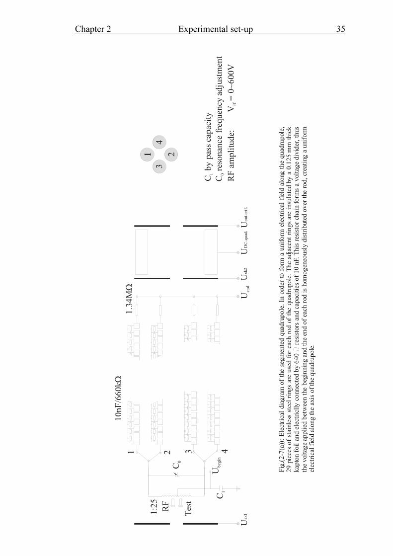
Fig.(2-6(a)): Schematic view of the segmented quadrupole. In order to form a uniform electrical field
along the quadrupole, 29 pieces of stainless steel rings are used for each rod of the quadrupole. The
adjacent rings are insulated by a 0.125 mm thick kapton foil and electrically connected by 640 Ω
resistors and capacities of 10 nF. This resistor chain forms a voltage divider, thus the voltage applied
between the beginning and the end of each rod is homogeneously distributed over the rod, creating a
uniform electrical field along the axis of the quadrupole.
Skimmer1 Skimmer2DC-quadrupole
Output orifice
RF quadrupole rods
DC-quadrupole rods
Trapping electrode
Fig.(2-6(b)): Schematic view of the LINAC quadrupole (PE SCIEX’s patent). Four additional tilted
rectangular rods are used to form a uniform electrical field along the axis of the quadrupole.
Chapter 2 Experimental set-up 35
Up
(Bla
ck)
RF
Test
C0
C re
sona
nce
freq
uenc
y ad
just
men
t0
23
41:
25
RF
ampl
itude
:
V
= 0
~600
Vrf
1.34
MΩ
C b
y pa
ss c
apac
ity1
1 2 3 4C
1U
begi
n
Uen
dU
sk2
UD
C-q
uad.
Uou
t.ori
f.U
sk1
10nF
/660
kΩ
Fig.
(2-7
(a)):
Ele
ctric
al di
agra
m o
f the
seg
men
ted
quad
rupo
le. I
n or
der t
o fo
rm a
uni
form
ele
ctric
al fi
eld
alon
g th
e qu
adru
pole
,29
pie
ces o
f sta
inle
ss st
eel r
ings
are
use
d fo
r eac
h ro
d of
the
quad
rupo
le. T
he a
djac
ent r
ings
are
insu
late
d by
a 0
.125
mm
thic
kka
pton
foil
and
elec
tricl
ly c
onne
cted
by
640
resis
tors
and
cap
aciti
es o
f 10
nF. T
his r
esist
or c
hain
form
s a v
olta
ge d
ivid
er, t
hus
the v
olta
ge ap
plie
d be
twee
n th
e be
ginn
ing
and
the e
nd o
f eac
h ro
d is
hom
ogen
eous
ly d
istrib
uted
ove
r the
rod,
cre
atin
g a u
nifo
rmel
ectri
cal f
ield
alon
g th
e ax
is of
the q
uadr
upol
e.W

Chapter 2 Experimental set-up 36
Up
(Bla
ck)
RF
Test
C0
C re
sona
nce
freq
uenc
y ad
just
men
t0
23
41:
25
RF
ampl
itude
:
V
= 0
~600
Vrf
C b
y pa
ss c
apac
ity1
1 2 3 4C
1U
begi
n
Uen
dU
sk2
UD
C-q
uad.
Uou
t.ori
f.U
sk1
Utr
ap
5 6 7 8
56 7
8
Fig.
(2-7
(b)):
Ele
ctric
al d
iagr
am o
f the
LIN
AC q
uadr
upol
e. In
ord
er to
form
a u
nifo
rm e
lect
rical
fiel
d al
ong
the
quad
rupo
le,
four
re
ctang
ular
ro
ds a
re u
sed
in a
dditi
on to
the r
ound
one
s. Ot
herw
ise, t
he el
ectri
cal d
iagra
m o
f the
LIN
ACqu
adru
pole
is si
mila
r to
the s
egm
ented
one
(see
Fig
.(2-7
(a)))
. til
ted
stain
less
stee
l

Chapter 2 Experimental set-up 37
The segmented and the LINAC quadrupoles have different longitudinal electrical
fields, which serve to drag the ions through the quadrupole. In the case of the
segmented quadrupole, in order to form a uniform electrical field, 29 pieces of
stainless steel rings are used for each rod of the quadrupole. The adjacent rings are
insulated by a 0.125 mm thick kapton foil and electrically connected by 640 Ω
resistors and capacities of 10 nF. This resistor chain forms a voltage divider, thus the
voltage (~1V) applied between the beginning and the end of each rod is
homogeneously distributed over the rod, creating an approximately uniform
electrical field along the axis of the quadrupole.
In case of the LINAC quadrupole four additional tilted rectangular rods are used to
form an approximately uniform electrical field along the axis of the quadrupole.
Otherwise, these two quadrupoles are identical. More detailed information about
mechanical and electrical realizations of the quadrupoles can be found in work
[Zhe00].
2.3 Einzel lens In Fig.(2-8) the time-of-flight analyzer(1) including the einzel lens(2) is shown
Fig.(2-8): Schematic view of the time-of-flight analyzer including an einzel lens and a MCP-detector.
The einzel lens is placed on the beam trajectory between the quadrupole and the entrance of the
accelerator. Like the quadrupole the einzel lens serves as a device that prepares the beam for the
further stage.

Chapter 2 Experimental set-up 38
The einzel lens is placed between the quadrupole and the entrance of the accelerator
(see Fig.(2-1) and Fig.(2-8)). The einzel lens serves as a device that converts the
angular divergence of the beam into the spatial spread of the beam. A schematic
view of the lens is shown in the Fig.(2-9(a)), the electrical diagram is presented in
Fig.(2-9(b)).
z
X
Fig.(2-9(a)): Schematic view of the einzel lens and its action on a beam
Ufocus
Udeflect
Fig.(2-9(b)): Electrical diagram of the einzel lens. Two potentials (Ufocus and Udeflect ) are applied to the
einzel lens. Thus, the einzel lens can focus as well as deflect a beam.

Chapter 2 Experimental set-up 39
The velocity spread ( ) and the spatial spread in z-direction ( ) (see Fig.(1-3))
are the main factors that affect the mass resolving power of the Ortho-TOF MS.
According to the Liouville theorem the phase space volume of the beam before and
behind the einzel lens is the same. A spatial spread of the ions in the modulator can
be compensated by the reflector, whereas a velocity spread can not be compensated
(see Appendix 1). Thus, the einzel lens is intended to widen the beam in the
modulator in order to reduce the velocity spread in z-direction (see Fig.(2-9(a))) and
therefore also the turn-around time. Since an ideal mechanical alignment can never
be achieved, the einzel lens is segmented in order to be able to adjust the direction of
the beam, in addition to its focusing property.
zν∆ z∆
2.4 The time-of-flight analyzer The time-of-flight analyzer (see Fig.(2-8)) can be functionally divided into three
parts: modulator-accelerator, drift region and reflector.
The basic principles of functioning of such TOF mass spectrometers are done in
subchapter 1.1 of chapter 1. Here is shortly considered only the technical realization
of the time-of-flight analyzer. A more detailed description of the time of flight
analyzer can be found in work [Zhe00]
Mountingplate
R C1 1
R C2 2
R C2 2
R C1 1
.........
Push plate(1)
Acceler.grid(5)
Beam
Modulator
Accelerator
Screening grid(2)
Metal plates(4)
Fig.(2-10): Schematic view of the modulator-accelerator[Zhe00]. The modulator is a region between
the push plate (1) and screening grid (2). The accelerator is a region between the pull grid (3) and the
accelerating grid (5). The set of metal plates forms a uniform electrical field (4). The working cycle of
the modulator-accelerator consists of two phases: Collecting the ions in the modulator and extraction
of the ions out of the modulator through the accelerator into the drift region by applying short pulses
of a voltage to the push plate and the pull grid.

Chapter 2 Experimental set-up 40
Fig.(2-11): A photo of the modulator.
The ion beam coming from the quadrupole and passing the einzel lens enters the
modulator (see Fig.(2-10) (schematic view of the modulator) and Fig.(2-11) (photo
of the modulator)). The modulator is a region between the push plate (1) and
screening grid (2). The accelerator is a region between the pull grid (3) and the
accelerating grid (5). The set of metal plates forms a uniform electrical field (4). The
working cycle of the modulator-accelerator consists of two phases: Collection of the
ions in the modulator and extraction of the ions out of the modulator through the
accelerator into the drift region by applying short pulses of a voltage to the push
plate and the pull grid.
During the next phase of ion collection, the new ions fill the modulator and
simultaneously the bunch of ions originating from the previous collection phase
passes the drift region, enters the reflector, gets reflected and hits the MCP-detector.
The drift region is held at an electric potential of –6000V. It is protected against
field penetration from outside by a metal screen. The potentials of about -300 V and
+1200 V are applied to the second grid and back plate respectively. A table with
typical values of geometrical parameters of the TOF-analyzer and the potentials
applied to the Ortho-TOF MS is presented in Appendix 5.

Chapter 2 Experimental set-up 41
Drift region
Reflector
The first grid
The second grid
Metal frames
Back plate
20 cm
32 cm
Fig.(2-12): The reflector of the time-of-flight analyzer. The homogeneous electrical fields in the
reflector, similarly as in the modulator-accelerator, are created by the set of metal frames, the first
grid at the entrance of the drift region, the second grid and the back plate. The first grid screens the
reflecting region from the field free drift region. The second grid divides the reflector into two regions
with different field strengths.
Fig.(2-13): A photo of the reflector.

Chapter 2 Experimental set-up 42
The homogeneous electrical fields in the reflector, similarly as in the modulator-
accelerator, are created in a set of metal frames. There are a first grid at the entrance
of the drift region and a second grid in the reflector (see Fig.(2-12) (schematic view
of the reflector) and Fig.(2-13) (photo of the reflector)). The first grid screens the
reflection region from the field free drift region. The second grid divides the reflector
into two regions with different electric field strengths.
2.5 Detection system The detection system consists of a detector and a data-acquisition system.
As a charged particle detector a chevron-type microchannel plate (MCP) detector is
used. A schematic view of the MCP-detector and the electrical diagram is presented
in Fig.(2-14). Fig.(2-15) is a photo of the MCP-detector. The position of the MCP-
detector in the Ortho-TOF MS is shown in Fig.(2-8).
MCP-plates
Signal to data-acquisition system
Drift space
6.5MΩ
3.8MΩ
1.9MΩ
3.8MΩ 0.38MΩ
-6kV
3kV
Anode
Fig.(2-14): MCP-detector, operated in a high voltage anode configuration. In the MCP-detector two
large micro channel plates (MCP) are used. The active area of each MCP is 60*40 mm , channel
diameter of 12µm, and bias angle of 8
2
0. The voltages are applied to each MCP through a resistor
divider. Since the MCP-detector is operated in a high voltage anode configuration, a decoupling
capacitor between the anode and the input of the data-acquisition system has to be used.

Chapter 2 Experimental set-up 43
Fig.(2-15): A photo of the MCP-detector used in the Ortho-TOF MS
In the MCP-detector two large micro channel plates (MCP) are used. The active area
of each MCP is 60*40 mm , the channel diameter is 12µm, and the bias angle is 82 0.
The voltages are applied to each MCP through a resistor divider. Since the MCP-
detector is operated in a high voltage anode configuration, a decoupling capacitor
between the anode and the input of the data-acquisition system has to be used.
In Table 4 the efficiency of a MCP as a function of the energy of incident ions is
listed [Pro00].
Energy Efficiency
ions
500eV ... 3keV
3keV ... 10keV
10keV ... 50keV
50keV ... 200keV
5% ... 40%
40% ... 70%
70% ... 80% ... 70%
70% ... 40%
Table 4: Efficiency of the a MCP vs. the energy of incident ion [Pro00]
The amplification of the MCP-detector is about 107 [Pro00].
Taking into account that the input impedance of the data-acquisition system is 50 Ω
one can estimate the average amplitude of the signal at the input of the data-
acquisition system.

Chapter 2 Experimental set-up 44
τQRV0 = (2_2)
Where Q is the charge at the anode, caused by one charged particle hitting the MCP-
detector, τ is the typical time-width of the charge signal at the anode, R is the input
impedance of the data-acquisition system.
Substituting typical values of R = 50 Ω, τ = 1ns, Q = 5*10 As values into
Eq.(2_2) one receives = 80 mV. Therefore, a preamplifier is required in order to
amplify the signal from a MCP-detector to the voltage level necessary for a data-
acquisition system.
13−
0V
Three different types of time-digital converters (TDC) are used in the data-
acquisition system in this work:
The Time-Digital Converter (TDC) (IONWERKS, Houston, USA)
The Picosecond Time Analyzer 9308(PTA) (ORTEC, USA)
The Time-Digital Converter 9353(TDC) (ORTEC, USA)
The configuration of the data-acquisition system is shown in Fig.(2-16). The
configuration is typical for time-of –flight applications. A pulse generator (National
Instrument delay generator computer built-in card) generates a start NIM-signal for
the TDC. As a stop signal the ion arrival signal from the MCP-detector is used. A
preamplifier is needed to amplify the signal from the MCP-detector for the next
stage. A constant fraction discriminator (CFD) should be used as an intermediate
stage before the TDC. It is defined by the following:
The amplitudes of the signals from the MCP-detector are not constant, after the pre-
amplification they range from several 100 mV up to 2V. In order to receive a high
resolving power of the Ortho-TOF MS an amplitude-insensitive converting device
such as a CFD should be used.
In this work a CFD 935 from ORTEC is used. Table 5 lists the main properties of the
TDCs.
Type of the TDC
Time-resolution
Dead time
TDC from IONWERKS 0.625 ns 20 ns
PTA 9308 from ORTEC Down to 1 ps 50 ns
TDC 9353 from ORTEC Down to 100 ps 1 ns
Table 5: The main properties of the TDCs used in the present work

Chapter 2 Experimental set-up 45
Generator of start TTL-signals (+5V)
Time-of-flight analzyer
Charge signal from the MCP-detector (~-25 mV, <1ns)
Fast preamplifier
Amplified signal (~up to -2V, <1ns)
Constant fraction discriminator Constant fraction discriminator
NIM-signal (-1V)stop signal for TDC
NIM-signal (-1V)start signal for TDC
Time to digit converter (TDC)
TOF-spectrum visualizing system (computer)+data storage
HV-pulser
Fig.(2-16): A schematic view of the configuration of the data-acquisition system. The configuration of
data-acquisition system is typical for time-of-flight applications. A pulse generator (National
Instrument delay generator computer built-in card) generates a start NIM-signal for the TDC. As a
stop signal a signal from the MCP-detector is used. A preamplifier is needed to amplify the signal
from the MCP-detector for the next stage. A constant fraction discriminator (CFD) is used before the
TDC in order to decrease the time jitter of the MCP signal.

Chapter 2 Experimental set-up 46
The PTA 9308 from ORTEC has the largest dead time and the highest time
resolution. So it is used at very low signal count rate of the MCP-detector. Due to the
very high time resolution, the PTA 9308 is best suited for the applications where a
high accuracy of mass determination is crucial. (Precision of determination of the
peak center of gravity depends on the number of time-bins in the mass peak).
The TDC 9353 from ORTEC has the shortest dead time and a time resolution which
is sufficient for many applications. So it is used at high signal count rate of the MCP-
detector when it is necessary to have a maximal efficiency of the Ortho-TOF MS.
The TDC from IONWERKS was the first TDC used in this work. Now it is used as a
spare system for the other two TDCs.
2.6 Vacuum system The vacuum system of the Ortho-TOF MS is double-staged or three-staged
according to the ion source used. When the electrospray ion source is used the
vacuum system is three-staged. Otherwise, it is double-staged. The schematic view
of the vacuum system is presented in Fig.(2-17(a,b)).
SEIKO SEIKI STP-400
Full-range gauge
Full-range gauge
Pirani gauge
TOF
10 mbar-7
5*10 mbar-5
10 mbar-2
quadrupoleElectrospray
Dry
nitr
ogen
Pirani gauge
1mbar
SEIKO SEIKI STP-400
VARIANTriScrollTM
EDWARDS E2M28
Fig.(2-17(a)): The vacuum system with electrospray ion source. It has three stages of differential
pumping in order to maintain the needed pressure in the Ortho-TOF MS.

Chapter 2 Experimental set-up 47
VARIANTriScrollTM
SEIKO SEIKI STP-400
Full-range gauge
Full-range gauge
Pirani gauge
TOF
10 mbar-7
5*10 mbar-5
10 mbar-2
quadrupoleIon source
Dry
nitr
ogen
SEIKO SEIKI STP-400
Fig.(2-17(b)): The vacuum system with Cs- or Laser- ion source. It has two stages of differential
pumping in order to maintain the needed pressure in the Ortho-TOF MS.


Chapter 3 Experimental results and discussion 48
Chapter 3
Experimental results and discussion
3.1 Investigation of cooling and trapping of the ions in the RFQ
The RFQ can be operated in two modes; in a continuous mode and bunch mode.
In the continuous mode the RFQ works as an ion cooler/guide. In the bunch mode
the ions after cooling are trapped at the end of the RFQ for a controlled time interval
and then extracted out of the RFQ in a well-confined bunch. The distribution of the
DC-electrical field along the RFQ for both modes is shown schematically in Fig.(3-
1). The green curve corresponds to the continuous mode and to the extraction stage
of the bunch mode. The red curve corresponds to the storage stage of the bunch
mode.
While the efficiency in the continuous mode due to the geometrical realization is
about three times lower than in the bunch mode, a broad mass range of a few
hundreds atomic mass units can be simultaneously investigated in the continuous
mode, where as in the bunch mode only a few tens of atomic mass units can be
covered.
The choice between these two modes is determined by the conditions of the
experiment to be conducted. For instance, at an on-line experiment at the SHIP at
GSI where the production rate of the ions of interest is very low and can amount to
several nuclides of interest per hour only the bunch mode should be used in order to
achieve the maximum efficiency. For other experiments where the production rate of
the nuclides of interest is high enough and the broad mass range is more important
than the high efficiency the continuous mode should be chosen.

Chapter 3 Experimental results and discussion 49
RF-quadrupole(Ion guide/linear Paul trap)
DC-potential Storage
Entrance Exit
Fig.(3-1): Schematic view of the distribution of the electrical DC-potential along the RFQ. The RFQ
can be operated in two modes; in a continuous mode and bunch mode. In the continuous mode the
RFQ works as an ion cooler/guide. In the bunch mode the ions after cooling are trapped at the end of
the RFQ for a controlled time interval and then extracted from the RFQ in the form of a well-confined
bunch.
In order to investigate the cooling and storage properties of the RFQ in both modes,
the test set-up shown in Fig.(3-2) was developed.
Iheating
Cs - fillement
RF-quadrupole(Ion guide/linear Paul trap)
Cs-ion source DC-quadrupole
MCP-detector
Retardation grids
to CFD
Suppression grids
Fig.(3-2): Test set-up for the investigation of the cooling and trapping properties of the RFQ. As the
test-RFQ a LINAC-type RFQ was chosen. The detection system consists of three parts: MCP-
detector, retardation grids and suppression grids. By varying the electrical potential applied to the
retardation grids one can measure the energy distribution of the ions.

Chapter 3 Experimental results and discussion 50
As the test-RFQ the LINAC-type RFQ was chosen. As ion source the Cs-surface
ionization ion source was used. It delivers an ion beam with a very stable ion current
up to a few µA. This gives the possibility to conduct quantitative investigations.
The detection system of the test system consists of three parts: a MCP-detector,
several retardation grids and several suppression grids.
The ions with a kinetic energy less than the potential energy defined by the
retardation grids potential are reflected by the retardation grids. The ions with a
kinetic energy higher than the potential energy defined by the retardation grids
potential can fly through the retardation grids and reach the MCP-detector. Thus, by
varying the electrical potential applied to the retardation grids one can measure the
kinetic energy and kinetic energy distribution of the ions. The detection efficiency of
the MCP-detector depends on the intensity of the ion beam hitting the MCP-detector.
Due to a saturation effect the detection efficiency drops at a high beam intensity. In
order to avoid this drop, and therefore an uncertainty in the detection efficiency, a set
of suppression grids can be inserted between the exit of the RFQ and the retardation
grids.
3.1.1 Continuous mode As it is shown in Chapter 4 the mass resolving power of the Ortho-TOF MS is
mainly limited by the turn-around-time which depends on the energy spread of the
ions after the cooling in the RFQ.
There are two effects that can influence the energy spread of the ions after the
cooling in the RFQ: gas pressure in the RFQ and RF-heating of the ions.
Investigation of the mean kinetic energy and the kinetic energy spread of the ions
after cooling vs pressure in the RFQ
The experimentally measured mean kinetic energy and kinetic energy spread
(FWHM) of the ions after cooling vs pressure in the RFQ are plotted in Fig.(3-
3(a,b)).

Chapter 3 Experimental results and discussion 51
2,0x10⁻² 4,0x10⁻² 6,0x10⁻² 8,0x10⁻² 1,0x10⁻¹ 1,2x10⁻¹
12,2
12,4
12,6
12,8
13,0
13,2
13,4
13,6
13,8
14,0
K (e
V)
He gas pressure (mbar)
Fig.(3-3(a)): The measured mean kinetic energy of the ions after cooling vs He pressure in the RFQ.
The errors of the measurements are smaller than the full circles.
2,0x10⁻² 4,0x10⁻² 6,0x10⁻² 8,0x10⁻² 1,0x10⁻¹ 1,2x10-10,0
0,5
1,0
1,5
2,0
∆K
(FW
HM
) (eV
)
He gas pressure (mbar)
Fig.(3-3(b)): The measured kinetic energy spread of the ions after the cooling and ejection from the
RFQ vs He pressure in the RFQ. The errors of the measurements are smaller than the full circles.

Chapter 3 Experimental results and discussion 52
From the measurements it can be seen that the mean kinetic energy of the ions drops
and the kinetic energy spread of the ions becomes broader with increase of the
pressure in the RFQ. This can be explained in the following way: The RFQ can be
divided into two regions with respect to strength of the electrical field applied along
the RFQ (see Fig.(3-4)).
Region 1(RFQ) DC-quadrupole
Ion beam
Region 2
Trapping el. Extracting el.
Fig.(3-4): The RFQ: In region 1 cooling of the ions takes place, region 2 is for fast ion extraction from
the RFQ. In region 1 the strength of the electrical field along the RFQ is very weak (E=0.05V/cm),
whereas in region 2 between the end of the RFQ, trapping electrode and extracting electrode, the
strength of the electrical field is very high (100V/cm).
In the first region the strength of the electrical field along the RFQ is very weak
(E=0.05V/cm) and serves for dragging the ions along the RFQ. The kinetic energy
distribution of the ions in region 1 is ~0.1 eV. In region 2 between the end of the
RFQ, trapping electrode and extracting electrode, the strength of the electrical field
is very high (100 V/cm). If the ions undergo collisions with the buffer gas in this
region their mean energy becomes lower and the energy spread becomes broader.
The more collisions they undergo the lower the mean energy and the broader the
energy spread of the ions extracted out of the RFQ. This explains the qualitative
behavior of the curves in Fig.(3-3(a,b)).
A typical energy spread of cooled ions in Region 1 is ~0.1 eV. From the
experimental curve it can be concluded that the pressure of He in the RFQ should not
exceed 2*10 mbar if one wants to keep the kinetic energy spread of the ions at the
level of the kinetic energy distribution of the buffer gas. This value should be the
2−

Chapter 3 Experimental results and discussion 53
upper limit for the He pressure in the RFQ when the Ortho-TOF MS is coupled to
the RFQ.
Cs-ion transmission through the RFQ vs the RF-potential applied to the RFQ
In Fig.(3-5) the measured transmission of the RFQ for Cs-ions is shown as a function
of the RF-potential applied to the RFQ. q-axis indicates Mathieu parameter (see
Eq.(1_24)). The parameters of the LINAC RFQ are following: radius r0=3.65 mm,
length L=40 cm, angular frequency Ω=1071/s.
50 100 150 200 250 300
0
200
400
600
800
1000
1200
0
200
400
600
800
1000
1200
0,1 0,2 0,3 0,4 0,5 0,6 0,7 0,8
num
ber o
f Cs+ io
ns (a
rbitr
ary
units
)
Vrf (V)
q
Fig.(3-5): Measured Cs-ion transmission through the RFQ vs the RF-potential. The q-axis indicates
the Mathieu parameter.
The transmission efficiency of the RFQ is low at low values of q due to a low value
of the pseudo-potential (see Eq.(1_22) and Eq.(1_24)), which accounts for the
focusing of the ions towards the RFQ-axis, stays constant at moderate values of q
and drops to zero at q-values close to 0.9, which corresponds to the onset of ion
motional instability.

Chapter 3 Experimental results and discussion 54
Investigation of the mean kinetic energy and the kinetic energy spread of the ions
after cooling vs RF-amplitude applied to the RFQ
The experimental mean kinetic energy and kinetic energy spread of the ions after the
cooling vs RF-potential of the RFQ are plotted in Fig(3-6(a,b)).
From the figures it can be seen that the mean kinetic energy of the ions increases
linearly and the energy spread of the ions becomes broader with an increase of RF-
amplitude.
50 100 150 200 250 30013,90
13,92
13,94
13,96
13,98
14,00
K (e
V)
Vrf (V)
Fig.(3-6(a)): The measured mean kinetic energy of the ions after cooling vs RF-potential applied to
the RFQ. The errors of the measurements are smaller than the full circles.

Chapter 3 Experimental results and discussion 55
50 100 150 200 250 300
0,11
0,12
0,13
0,14
0,15
0,16
0,11
0,12
0,13
0,14
0,15
0,16
0,2 0,3 0,4 0,5 0,6 0,7 0,8q
∆K (F
WH
M) (
eV)
Vrf (V)
Fig.(3-6(b)): The measured kinetic energy spread of the ions after cooling vs RF-amplitude applied
to the RFQ. The errors of the measurements are smaller than the full circles. The q-axis indicates the
Mathieu parameter. The drastic increase of the kinetic energy spread at higher RF-amplitude, i.e. at
higher Mathieu parameter, is due to RF-field heating of the ions and agrees with the theory [Daw76]
From the theory of the cooling in a RFQ (see chapter 1, subchapter 1.2.2) is known
that the ions in a RFQ are subject to two different effects: (1) cooling effect: due to
the collisions of the ions with the buffer gas the energy spread of the ions tends to
reach the doubled energy spread of the buffer gas and (2) heating effect: the ions
gain some amount of energy from the RF-field. The heating effect starts to play a
significant role only when q (see Eq.(1_24)) is higher than 0.8. Below this value the
cooling effect dominates and heating effect can be neglected.
The rise of the mean energy of the ions after cooling with respect to RF-amplitude
can be explained by a slight asymmetry of the RF-potential. The energy spread of the
ions after cooling is constant for q<0.4 and equals ~0.11 eV and grows drastically
for q>0.7, which is in agreement with the theory [Daw76]. The following conclusion
can be derived:
The RFQ should be operated at q-values between 0.35 and 0.6 in order to: (1) avoid
a low transmission efficiency of the ions through the RFQ and (2) to achieve the
most effective cooling of the ions in the RFQ.

Chapter 3 Experimental results and discussion 56
3.1.2 Bunch mode
Investigation of ions time of flight through the RFQ vs pressure in the RFQ
The overall time of flight of the ions from the entrance of the RFQ to the MCP-
detector of the Ortho-TOF MS ( ) is a very important characteristic. Only
nuclides with half-life longer than can be efficiently investigated with the
Ortho-TOF MS. The time of flight of the ions through the RFQ dominates in
.
overallflightt
overallflightt
RFQflightt
overallflightt
The goal is to minimize . This can be achieved by varying the pressure in the
RFQ. The experimental set-up is shown in Fig.(3-2). The timing diagram of the
measurement is presented in Fig.(3-7). The output electrode of the Cs-ion source can
be pulsed. When a potential of ~ +25V is applied, the ion source is closed (V
RFQflightt
ion source
corresponding to “closed” level in Fig.(3-7) ). Switching the ion source potential
down to zero ((Vion source corresponding to “open” level in Fig.(3-7)) a bunch the Cs-
ions is extracted. Making a scan of the trapping time of the linear RFQ trap (see
Fig.(3-7)) one obtains the number of ions reaching the linear RFQ trap as a function
of the trapping time (see Fig.(3-8)). The time of flight of the Cs-ions through the
RFQ corresponds to the saturation of the curve. Making the same procedure for
different He pressures in the RFQ one obtains the time of flight of the ions through
the RFQ as a function of the He pressure in the RFQ (see Fig.(3-9)).

Chapter 3 Experimental results and discussion 57
tin t ~storage 0,5-10 ms
Vion source
+25V closed
open
Vtrapping
+20V closed
open
t
Fig.(3-7): Timing diagram for the investigation of the ions flight-time through the RFQ. The output
electrode of the Cs-ion source can be switched. When a potential of ~ +25V is applied, the ion source
is closed (Vion source corresponding to “closed” level). Switching the ion source potential down to zero
((Vion source corresponding to “open” level) one can bunch the Cs-ion source beam. By scanning the
trapping time of the linear RFQ trap one obtains the number of ions reaching the linear RFQ trap as a
function of the trapping time.
0 1 2 3 4 5 6 7 8 9 100,0
0,1
0,2
0,3
0,4
0,5
0,6
0,7
0,8
0,9
1,0
1,1
tRFQflight
num
ber o
f ion
s in
the
linea
r RFQ
trap
(arb
itrar
y un
its)
ttrapping (ms)
Fig.(3-8): Measured number of ions reaching the linear RFQ trap as a function of the trapping time of
the linear RFQ trap for a He pressure of 3*10-2 mbar in the RFQ.

Chapter 3 Experimental results and discussion 58
0,0 5,0x10⁻³ 1,0x10⁻² 1,5x10⁻² 2,0x10⁻² 2,5x10⁻²⁰
1
2
3
4
5
tRFQ
fligh
t (ms)
PHe (mbar)
Fig.(3-9): Measured time of flight of the ions through the RFQ vs the He pressure in the RFQ. The
errors of the measurements are smaller than the full circles. The curve has a minimum
at a pressure . At this pressure the ions are cooled right at the
exit of the RFQ after one pass (the RFQ length is 40 cm, the kinetic energy of the incoming ions is
about 4 eV). At lower pressure the ions make several passes until they are cooled. At higher pressure
the ions are already cooled somewhere in the RFQ and slowly drift to the exit of the RFQ.
ms.t RFQimummin 50= mbar* 3108 −
The curve has a minimum at a pressure . At this
pressure the ions are cooled right at the exit of the RFQ after one pass (the RFQ
length is 40 cm, the kinetic energy of the incoming ions is about 4 eV). At lower
pressure the ions make several passes until they are cooled. This explains why
at lower pressure is longer than . At higher pressure the ions are already
cooled somewhere in the RFQ and slowly drift to the exit of the RFQ.
ms.t RFQimummin 50= mbar* 3108 −
RFQflightt
RFQimummint
It can be concluded that the time property of the TOF allows to investigate the
nuclides with half-life longer than 0.5 ms, the pressure should be
chosen as an optimal pressure of He in the RFQ.
mbar* 3108 −
Investigation of the ion storage capacity of the linear RFQ trap
According to the calculation presented in Appendix 3 the ion storage capacity of the
linear RFQ trap (the number of ions which can be stored in the linear RFQ trap)
amounts to about 2*105 singly charged ions. Usually only a few ions of interest will

Chapter 3 Experimental results and discussion 59
be stored in the linear RFQ trap during an on-line experiments with exotic ions. But
besides the ions of interest many contaminant nuclides are produced and not
separated in the in-flight separator, therefore, the total production rate of all nuclides
can become comparable with the ion capacity of the linear RFQ trap. Therefore, and
investigation of the ion capacity of the linear RFQ trap is required.
In Fig.(3-10) the experimental dependence of the number of the ions n stored in the
linear RFQ trap on the number of the ions injected into the RFQ is presented. The
measurement procedure was similar to that for the flight time of the Cs-ions through
the RFQ except that the He pressure in the RFQ and the trapping time were kept
constant to 1*10-2 mbar and 1ms, respectively (optimum pressure and trapping time;
see Fig.(3-9)). As can be seen from Fig.(3-10), the trapping efficiency of the linear
RFQ trap is almost 100% for up to 5*104 ions injected into the RFQ. For larger
number of ions injected into the RFQ the space charge of the ions trapped in the
linear RFQ trap becomes significant, and this limits the capacity of the linear RFQ
trap to about 1,4*105 ions.
0,0 5,0x10⁴ 1,0x10⁵ 1,5x10⁵ 2,0x10⁵ 2,5x10⁵ 3,0x10⁵
0,0
2,0x10⁴
4,0x10⁴
6,0x10⁴
8,0x10⁴
1,0x10⁵
1,2x10⁵
1,4x10⁵
1,6x10⁵
num
ber o
f ion
s st
ored
in
the
linea
r RFQ
trap
the number of ions injected into the RFQ
Fig.(3-10): Experimental dependence of the number of the ions n stored in the linear RFQ trap on the
number of the ions injected into the RFQ. The ion capacity of the linear RFQ trap (the number of the
ions which can be stored in the linear RFQ trap) amounts to about 1.4*105 ions and limited by space
charge repulsion of the ions in the linear RFQ trap.

Chapter 3 Experimental results and discussion 60
From the SIMION simulation (see Fig.(A3-5), Appendix 3) it can be seen that the
linear RFQ trap can efficiently store up to 2.2*10 ions. The experimental
measurement gives 1.4*10 5 ions. Taking into account that the errors of the
measurement of the absolute number of the Cs-ions and the SIMION simulation are
estimated to lie in a range of about a hundred percents one can conclude that the
experimental measurement is in agreement with the SIMION simulation.
5
Investigation of the mean kinetic energy and the kinetic energy spread of the ions
extracted from the linear RFQ trap vs the number of the ions stored.
In this subchapter the mean kinetic energy and the kinetic energy spread of the ions
extracted out of the linear RFQ trap are investigated. The experimental results of the
mean kinetic energy and the kinetic energy spread of the ions extracted out of the
linear RFQ trap are shown in Fig.(3-11).
1
2
3
0,0 2,0x10⁴ 4,0x10⁴ 6,0x10⁴ 8,0x10⁴ 1,0x10⁵ 1,2x10⁵ 1,4x10⁵
number of ions in the trap
∆K (
eV)
measured energy spread of the ions in the trap SIMION simulation of the energy spread
0,0 2,0x10⁴ 4,0x10⁴ 6,0x10⁴ 8,0x10⁴ 1,0x10⁵ 1,2x10⁵ 1,4x10⁵ 1,6x10510,0
10,2
10,4
10,6
10,8
11,0
11,2
11,4
11,6
11,8
12,0
K (e
V)
number of ions in the trap
Fig.(3-11): Measured mean kinetic energy (red curve), measured kinetic energy spread (blue curve)
and SIMION simulation of kinetic energy spread (black curve) of the ions extracted from the linear
RFQ trap
It should be noted that in the bunch mode the kinetic energy spread of the ions
extracted out of the RFQ is defined by their spatial distribution in the linear RFQ
trap (see Fig.(A3-3) in Appendix 3). The experimentally measured mean kinetic
energy does not depend on the number of ions stored in the linear RFQ trap, which is
in agreement with the Fig.(A3-3) in Appendix 3. The experimentally measured mean

Chapter 3 Experimental results and discussion 61
energy (11.05± 0.05 eV) and the mean energy derived from Fig.(A3-3) (11.1 eV) are
in perfect agreement with each other.
The ions due to their quasi-thermal kinetic energy distribution occupy a certain
minimum volume in the RFQ trap until their number exceeds
(Appendix 3) and space charge effect starts to push them
away from each other, increasing the space they occupy and, as a result, the kinetic
energy spread of the ions extracted out of the linear RFQ trap. As one can see the
behavior of the experimental curve (Fig.(3-11) blue curve) agrees with the expected
behavior of the ions in the linear RFQ trap mentioned above. Let us do a quantitative
comparison:
4105*n effect_eargch_no ≅
It can be seen from Fig.(A3-3) that the kinetic energy spread of the extracted ions is
a function of (see Appendix 3 for the definition of ) and, thus, a
function of the number of the ions. From Fig.(A3-3) this function can be derived:
trappingU trappingU
2trappingtrapping U*65U*40.51.8K −+−=∆ [eV] (3_1)
where ranges from 0.1eV to 0.5eV. For <0.1eV one obtains trappingU trappingU
K∆ =1.6eV.
Combining Eq.(3_1) and Eq.(A3_8) one can find the following dependence which is
plotted in Fig.(3-11).
The SIMION simulation increases more steeply with the number n of ions. While
Eq.(A3_8) does not correctly describe the ‘tail’ part of the linear RFQ trap (large
values of n) (see Appendix 3, Fig.(A3-6)), the central part of the linear RFQ trap
(low values of n) is well described. Since, only the shape of the central part of the
RFQ trap is important for our applications one can conclude that the SIMION-
simulation predicts the behavior of the linear RFQ trap correctly.
Investigation of the storage time of the ions in the linear RFQ trap vs impurity
pressure in the RFQ
The storage time Tstorage of the ions in the linear RFQ-trap can be defined as the time
after which only half of the initial quantity of the ions remains in the trap. There are

Chapter 3 Experimental results and discussion 62
several conditions which determine the storage time:(1) space charge effects, (2)
mechanical imperfection of the RFQ and (3) charge exchange collisions of the ions
with impurities in the buffer gas He and, therefore, neutralization of the ions.
Since we consider here only a small number of ions stored in the linear RFQ trap,
space charge effects can be neglected. The impurity pressure (the pressure of
residual gases and water vapors in He) was varied from up to .
The experimental dependence of the storage time from the impurity level is
presented in Fig.(3-12). As expected, the storage time drops with increasing impurity
pressure (a sum of the O
mbar510− mbar310−
2, N2 and H2O partial pressures). This indicates that the
collisions of the ions with impurities does lead to significant reduction of the storage
time. Unfortunately, there is a lack of the experimental data on charge-exchange
cross-sections in sub-eV and eV kinetic energy ranges. Thus, we have to rely on
model calculations. These calculations are done below.
1E-5 1E-4 1E-3
200
400
600
800
1000
1200
1400
Tst
orag
e (ms)
impurity pressure (mbar)
Fig.(3-12): Measured storage time of the Cs-ions in the linear RFQ trap vs the impurity pressure in
the RFQ. The impurity pressure implies the pressure of residual gases and water vapors in He (O2, N2
and H2O).
Charge-changing collisional processes taking place in a gas are listed in Table 6
[Has72].
Process Equation
Single charge transfer ++ +→+ BABA
Transfer ionization eBABA ++→+ ++ 2
Stripping BeABA ++→+ ++ 2

Chapter 3 Experimental results and discussion 63
Charge transfer to an excited level ++ +→+ BABA ' , '++ +→+ BABA
Capture by neutral atom +− +→+ BABA
Collisional detachment BeABA ++→+−
Table 6: Charge-changing collisional processes taking place in a gas. are the projectile and
target ions, respectively. are the projectile and target neutrals respectively. A prime is
inserted if one of the systems is excited and the symbol e is used if an electron is ejected [Has72]
++ BA ,
BA ,
The kinetic energy of Cs-ions undergoing collisions with the buffer gas in the RFQ
is around 0.1 eV, thus transfer ionisation and stripping can not occur because the
ionisation potentials of the colliding ions or neutrals are large compared to the
kinetic energy. Collisional detachment takes place only when one of the colliding
ions is negative. Thus, charge transfer is predominant in our case [Has72].
Two different charge transfer processes can take place [Has72]: (1) Symmetrical
resonance charge transfer and (2) Charge transfer between unlike ions and atoms.
Symmetrical resonance charge transfer takes place between two ions or atoms of the
same kind. That is not our case.
In our case the Cs-ions collide with the buffer gas, which is He and with impurities,
which are mostly N , O and water, thus only charge transfer between unlike ions
and atoms should be taken into account .
2 2
The adiabatic criterion proposed by Massey [Mas49] is important in these collisions:
hEa
vaΔ
= (3_2)
where is the impact velocity, a is known as the ‘adiabatic parameter’, a distance
of the order of atomic dimensions over which the charge transfer transition is
significant,
av
EΔ is the difference between the ionization potentials of colliding ions
and atoms, h is the Plank constant.
The kinetic energy that corresponds to is much larger than 1 eV for all charge
transfer processes between unlike ions and atoms. Below this energy collisions are
called ‘adiabatic’. In this region the relative motion of the atoms is so slow that
charge transfer becomes a very unlikely event [Has72]. The collisions of Cs-ions
av

Chapter 3 Experimental results and discussion 64
with the buffer gas can be characterized as ‘adiabatic’. The cross-section σ of an
‘adiabatic’ collision can be approximated as follows [Has72]:
i4
EEvFσ ⎟⎠⎞
⎜⎝⎛≅∆
(3_3)
where is the impact velocity, F is a constant defined in [Has72] and Ev i is the
ionization potential of the projectile ion.
The direct calculation of the cross-section from Eq.(3_3) can lead to a large error
because the theory on which Eq.(3_3) is based is simplified. Instead, one can scale
experimentally determined cross-sections to the required conditions, using Eq.(3_3).
In our case charge transfer reaction of Cs
σ
+ ions with He, O2, N2 and H2O can occur.
From Eq.(3_3) one has for this case
iB
iCs
4
ACs
CB4
CB
ACs
CB
ACs
E
EEE
vv
σσ
+
+
+
+
+
+
+
+
⎟⎟⎠
⎞⎜⎜⎝
⎛⎟⎟⎠
⎞⎜⎜⎝
⎛=
+
+
+
+
+
+
ΔΔ
(3_4)
where A, B+, C are the ions and atoms undergoing the charge transfer reactions and
Ei is the first ionization potential of the ion or atom considered.
The reactions that are considered are listed in Table 7. The buffer gas is assumed to
be at rest. Thus, the impact velocity is assumed to be the velocity of incident ions
(0.1eV).
reaction B+ C KB+
+C, eV EiB
+, eV EiC, eV σ , cm2 Ref
Ne++Ar Ne+ Ar 0.1 21.564 15.73 10-19 [Has72]
Cs++Al Cs+ Al 0.1 3.89 5.986 <10-19 [Rut81]
Cs++Fe Cs+ Fe 0.1 3.89 7.87 <10-19 [Rut81]
Table 7: Data on reference reactions used in the storage time estimation. KB
++C is the kinetic energy of
relative motion of B+ and C that corresponds to in Eq.(3_4). CBv ++
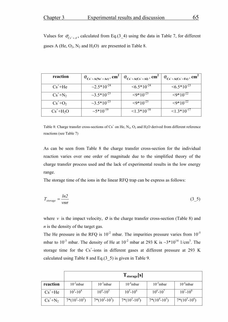
Chapter 3 Experimental results and discussion 65
Values for ACsσ ++ , calculated from Eq.(3_4) using the data in Table 7, for different
gases A (He, O2, N2 and H2O) are presented in Table 8.
reaction Ar)A(NeCsσ ++ ++ , cm2Al)A(CsCsσ ++ ++ , cm2
Fe)A(CsCsσ ++ ++ , cm2
Cs++He ~2.5*10-24 <6.5*10-24 <6.5*10-23
Cs++N2 ~3.5*10-23 <9*10-23 <9*10-22
Cs++O2 ~3.5*10-23 <9*10-23 <9*10-22
Cs++H2O ~5*10-19 <1.3*10-18 <1.3*10-17
Table 8: Charge transfer cross-sections of Cs+ on He, N2, O2 and H2O derived from different reference
reactions (see Table 7)
As can be seen from Table 8 the charge transfer cross-section for the individual
reaction varies over one order of magnitude due to the simplified theory of the
charge transfer process used and the lack of experimental results in the low energy
range.
The storage time of the ions in the linear RFQ trap can be express as follows:
σnvln2Tstorage = (3_5)
where is the impact velocity, v σ is the charge transfer cross-section (Table 8) and
n is the density of the target gas.
The He pressure in the RFQ is 10-2 mbar. The impurities pressure varies from 10-5
mbar to 10-3 mbar. The density of He at 10-2 mbar at 293 K is ~3*1014 1/cm3. The
storage time for the Cs+-ions in different gases at different pressure at 293 K
calculated using Table 8 and Eq.(3_5) is given in Table 9.
Tstorage[s]
reaction 10-2mbar 10-3mbar 10-4mbar 10-5mbar 10-6mbar
Cs++He 103-104 104-105 105-106 106-107 107-108
Cs++N2 7*(101-102) 7*(102-103) 7*(103-104) 7*(104-105) 7*(105-106)
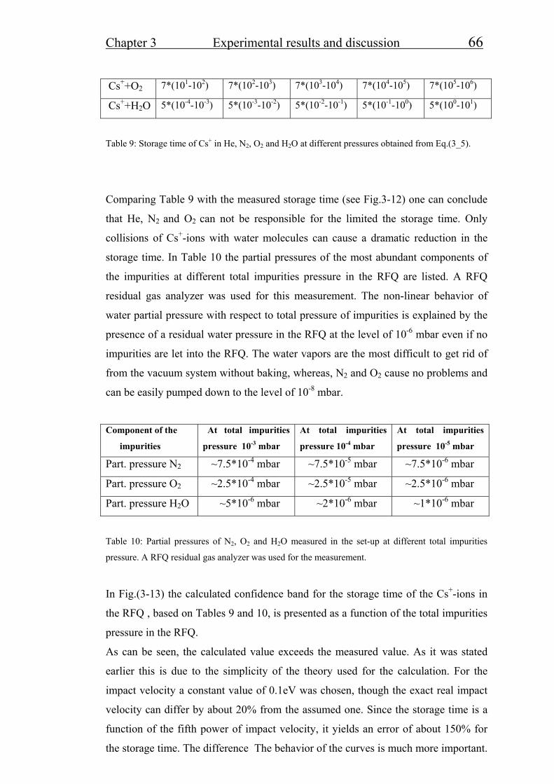
Chapter 3 Experimental results and discussion 66
Cs++O2 7*(101-102) 7*(102-103) 7*(103-104) 7*(104-105) 7*(105-106)
Cs++H2O 5*(10-4-10-3) 5*(10-3-10-2) 5*(10-2-10-1) 5*(10-1-100) 5*(100-101)
Table 9: Storage time of Cs+ in He, N2, O2 and H2O at different pressures obtained from Eq.(3_5).
Comparing Table 9 with the measured storage time (see Fig.3-12) one can conclude
that He, N2 and O2 can not be responsible for the limited the storage time. Only
collisions of Cs+-ions with water molecules can cause a dramatic reduction in the
storage time. In Table 10 the partial pressures of the most abundant components of
the impurities at different total impurities pressure in the RFQ are listed. A RFQ
residual gas analyzer was used for this measurement. The non-linear behavior of
water partial pressure with respect to total pressure of impurities is explained by the
presence of a residual water pressure in the RFQ at the level of 10-6 mbar even if no
impurities are let into the RFQ. The water vapors are the most difficult to get rid of
from the vacuum system without baking, whereas, N2 and O2 cause no problems and
can be easily pumped down to the level of 10-8 mbar.
Component of the
impurities At total impurities
pressure 10-3 mbar
At total impurities
pressure 10-4 mbar
At total impurities
pressure 10-5 mbar
Part. pressure N2 ~7.5*10-4 mbar ~7.5*10-5 mbar ~7.5*10-6 mbar
Part. pressure O2 ~2.5*10-4 mbar ~2.5*10-5 mbar ~2.5*10-6 mbar
Part. pressure H2O ~5*10-6 mbar ~2*10-6 mbar ~1*10-6 mbar
Table 10: Partial pressures of N2, O2 and H2O measured in the set-up at different total impurities
pressure. A RFQ residual gas analyzer was used for the measurement.
In Fig.(3-13) the calculated confidence band for the storage time of the Cs+-ions in
the RFQ , based on Tables 9 and 10, is presented as a function of the total impurities
pressure in the RFQ.
As can be seen, the calculated value exceeds the measured value. As it was stated
earlier this is due to the simplicity of the theory used for the calculation. For the
impact velocity a constant value of 0.1eV was chosen, though the exact real impact
velocity can differ by about 20% from the assumed one. Since the storage time is a
function of the fifth power of impact velocity, it yields an error of about 150% for
the storage time. The difference The behavior of the curves is much more important.

Chapter 3 Experimental results and discussion 67
Comparing the experimental curve (see Fig.(3-12)) and calculated curves, one can
see almost identical behavior: in both cases the storage time drops with a factor of 6
as the impurities pressure rises by a factor of 100. Thus, the losses of Cs+-ions in the
RFQ are most probably caused by collisions with the water molecules in the RFQ.
1E-5 1E-4 1E-3
1
10
100
stor
age
time
(s)
impurities pressure (mbar)
Fig.(3-13): Calculated confidence band for the storage time (see Eq.(3_5)) of the Cs+-ions in the
linear RFQ trap vs the impurity pressure (H2O, O2, N2) in the RFQ. The storage time is limited by
charge transfer reaction between Cs+-ions and water. The charge transfer cross-section for this
reaction (see Table 8) is calculated from Eq.(3_4) for different reference reactions (see Table 7).
Conclusion:
The storage time of Cs+-ions in the RFQ at a water partial pressure of 10-6 mbar is
more than 1s. Cs is the best element for long storage times due to its low first
ionization potential (3.89 eV). The first ionization potentials of most elements range
from 3.89 eV to ~15 eV [Nuc00]. The storage time for an element with a high first
ionization potential (~15 eV) reduces to a value of about 20 ms at a water partial
pressure of 10-6 mbar. The storage time for an element with a high first ionization
potential is much longer than the cooling time of the ions in the RFQ (<1ms). This
means that all elements can be cooled in the RFQ without significant charge
exchange losses. If some applications require longer storage times, one should
reduce the water partial pressure. This can be done easily down to the level of 10-7
mbar by purging the RFQ vacuum chamber with a dry gas like Ar. Further reduction

Chapter 3 Experimental results and discussion 68
takes a long time for pumping of the RFQ. The process can be sped up by baking the
RFQ vacuum chamber.
3.2 Precision of mass determination The accuracy of mass determination ∆M/M and the precision of mass determination
∆(∆M/M) can be defined as follows:
litMMmeslit MMM −
=∆
2σ
∆M
M
2
lit
mes2
2lit
litmes
MM
MMM
)MM( ⎟⎟
⎠
⎞⎜⎜⎝
⎛+⎟
⎟⎠
⎞⎜⎜⎝
⎛=
∆∆
∆∆ (3_6)
where Mlit and ∆Mlit are the literature value and its error of the nuclide mass, Mmes and
∆Mmes are the most probable value and standard error of the nuclide mass
determination measured with the Ortho-TOF MS. Since |∆Mmes| >> |∆Mlit | for the
Ortho-TOF MS, the expression for ∆AM can be rewritten as follows:
litmes /MM)MM( ∆=
∆∆ (3_7)
The procedure of mass determination consists of several steps: (1) The acquisition of
a TOF-spectrum, (2) the mass-calibration of the acquired TOF-spectrum and (3) the
determination of the unknown masses of interest in the TOF-spectrum.

Chapter 3 Experimental results and discussion 69
Measured TOF-spectra
A typical TOF-spectrum is shown in Fig.(3-14). After fitting with a Gaussian
distribution with a small tail on the right side (see in-set in Fig.(3-14) ) one obtains
the following parameters:
t is the most probable value of the time-of-flight of the nuclide of a given mass
σ is its standard deviation
∆t is the standard error of t determination, which is ~ nσ , where n is the number of
counts in the peak.
15000 20000 25000 30000 35000 400000
1000
2000
3000
4000
5000
6000
coun
ts
TOF (ns)
Fig. (3-14): A typical TOF-spectrum, measured with the Ortho-TOF MS. After fitting with a Gaussian
distribution including a small tail on the right side one obtains the following parameters:
t is the most probable value of the time-of-flight of the nuclide of a given mass
σ is its standard deviation
∆t is the standard error of t identification, which is ~ nσ
, where n is the number of counts in the
peak.

Chapter 3 Experimental results and discussion 70
Doing the same procedure for every peak in the spectrum one can obtain t and ∆t for
each peak in the spectrum:
nn
22
11
tt...........tttt
Δ
ΔΔ
±
±±
(3_8)
The mass-calibration
The next step is the mass calibration of the TOF-spectrum. The mass of the nuclide
as a function of its time-of-flight can be driven from the theoretical Eq.(1_1).
2AtM = (3_9)
In Eq.(3_9) an additional parameter (B) should be added due to time delays of
signals occurring in the data acquisition system. The function, which is used for the
mass calibration, is given by Eq.(3_10):
2B)-A(tM = (3_10)
For the mass calibration one chooses several reference peaks, which correspond to
nuclides with known masses Mlit. By using a least-square fitting procedure one can
get for A and B:
fitfitfitfit BBB and AAA ΔΔ ±=±= (3_11)
Substituting Afit and Bfit in Eq.(3_10) one can obtain the following expression for the
identification of unknown masses:
(3_12) 2fitfitexp )B-(tAM =
The standard deviation and weight error of Mexp are functions of t,Afit, Bfit, ∆Afit and
∆Bfit,
Chapter 3 Experimental results and discussion 71
∆Mstandard = F1(T,Afit, Bfit, ∆Afit,∆Bfit)
∆Mweight = F2(T,Afit, Bfit, ∆Afit,∆Bfit) (3_13)
and can be calculated by using the matrix method [Dge74]. As ∆Mexp one should
take the maximal error [Dge74]:
∆Mexp = max[∆Mstandard, ∆Mweight] (3_14)
Substituting Mexp into Eq.(3_6) and ∆Mexp in Eq.(3_7) one can obtain
)MM(M
M ∆∆±∆ for the nuclide of interest.
Determination of unknown masses in the TOF-spectrum
There are two kinds of calibration: (1) External and (2) internal.
An internal calibration implies a presence of reference peaks in the recorded TOF-
spectrum. But more often at on-line measurements there are no well-known nuclides
in the TOF-spectrum. In this case one has to make a mass calibration before the on-
line measurement (externally). An external calibration brings an additional error into
the measurement. In order to overcome this problem we are planning to use a
fullerene (C60) laser ion source for internal calibration of the Ortho-TOF MS at on-
line experiments. The development of this source is the subject of the doctoral thesis
of Z.Wang. The source covers the whole TOF-spectrum with known masses with an
interval of 12 atomic mass units, if the fullerene target is used with natural carbon
isotope ratios, and with intervals of 1 atomic mass unit, if the fullerene source is
enriched with 13C.
Internal calibration:
An investigation of the internal calibration was performed for two extreme cases:
(1) The reference peaks are situated close to the unknown peak in the TOF-spectrum
and (2) the reference peaks are situated far from the unknown peak in the TOF-
spectrum.
The second case was investigated in Munich with a silver beam (107Ag1+) from the
tandem. The experiment and its results are described in the following chapter. The

Chapter 3 Experimental results and discussion 72
investigation of the first case was carried out with three isotopes of Pb
(206Pb1+,207Pb1+,208Pb1+).
The source of the Pb-isotopes was the electrospray ion source. 207Pb1+ was used as an
unknown nuclide, and 206Pb1+ and 208Pb1+ were used as reference peaks. The distance
between the unknown peak and the reference peaks is about 1 mass unit. The TOF-
spectrum of the Pb-isotopes is shown in Fig.(3-15). In Table 11 the tabulated values
of the Pb-isotopes are presented [Nuc00]. 23 spectra were acquired. For each
spectrum the mass accuracy and precision )MM(M
M ∆∆±∆ were calculated.
Fig.(3-16) is a plot of these 23 measurements where the red line is the most probable
value of MM∆ (-0.2 ppm), the blue lines represent the 67%-confidence band of
MM∆ (0.51 ppm).
TOF (ns) Fig.(3-15): Time-of-flight spectrum of Pb-isotopes acquired with the Ortho-TOF MS. The mass of
207Pb was determined, 206Pb and 208Pb were used as reference peaks.

Chapter 3 Experimental results and discussion 73
0 5 10 15 20 25
-2,0
-1,5
-1,0
-0,5
0,0
0,5
1,0
1,5
2,0
AM (
ppm
)
Measurement number
Fig.(3-16): Accuracy of mass determination of 207Pb1+. It is a plot of these 23 measurements where the
red line is the most probable value of MM∆ , the blue lines are a 67%-confidence band of
MM∆ .
Pb- isotope Tabulated mass in atomic units 206Pb1+ 205.9738914 207Pb1+ 206.9753314 208Pb1+ 207.9760814
Table 11: Tabulated values of the Pb-isotopes[Nuc00]. One electron mass is subtracted.
:
The precision of the mass determination lies below 1 ppm, that corresponds to± 100
keV of the absolute error of the mass measurement of 207Pb. The accuracy of the
mass determination (systematic error) of 207Pb is 40 keV.

Chapter 3 Experimental results and discussion 74
3.3 Investigation of the Efficiency and Mass Resolving Power
of the Ortho-TOF MS
3.3.1 Efficiency of the Ortho-TOF MS
In order to measure the efficiency of the Ortho-TOF MS, the Cs+-ion source was
used. It delivers a very stable beam of Cs+-ions (see Fig.(2-4)). The efficiency of the
Ortho-TOF MS was measured for both the continuous mode and the bunch-mode.
The RFQ was adjusted to the maximum transmission of Cs+-ions (see Fig.(3-5)). In
Fig.(3-17) the efficiency of the Ortho-TOF MS for both modes as a function of the
MCP-detector voltage is presented.
2200 2300 2400 2500 2600 2700 28000,00,20,40,60,81,01,21,41,61,82,02,22,42,62,83,03,23,4
Effic
ienc
y (%
)
MCP-detector voltage (V)
bunch mode
continuous mode
Fig. (3-17): Mmeasured efficiency of the Ortho-TOF-MS in the bunch and continuous modes vs the
MCP-detector voltage.

Chapter 3 Experimental results and discussion 75
The maximum measured efficiency amounts to 3 % in the bunch mode and 1% in the
continuous mode.
From Fig.(3-17) it can be seen that the higher the MCP-detector voltage is the higher
the efficiency of the Ortho-TOF MS is. On the other hand, the higher MCP-detector
voltage yields a worse ratio of signal to noise. In Fig.(3-18) the number of noise
counts per second in a 10 ns interval of a TOF-spectrum is shown vs the MCP-
detector voltage for different He pressure in the Ortho-TOF MS.
2300 2400 2500 2600 2700 2800
0,0
5,0x10⁻³
1,0x10⁻²
1,5x10⁻²
2,0x10⁻²
nois
e co
unts
per
sec
ond
in 1
0ns
MCP-detector voltage (V)
PHe=1.1*10-5mbar
PHe=4.4*10-6mbar
PHe=3.0*10-6mbar
PHe=9.0*10-7mbar
PHe=1.0*10-7mbar
Fig.(3-18): Measured noise properties of the Ortho-TOF MS vs the MCP voltage for different He
pressure.
Since a typical peak width at 1% height is around 10 ns, in Fig.(3-18) the number of
noise counts per second in 10 ns (in the peak) is used as a measure for the signal-to-
noise study. From Fig.(3-17) and Fig.(3-18) it can be seen that the noise counts grow
exponentially with the MCP-detector voltage whereas the efficiency grows linearly.
In Fig.(3-19) the measured number of noise counts per second in 10 ns is shown vs

Chapter 3 Experimental results and discussion 76
the He pressure in the Ortho-TOF MS at the maximum efficiency of the Ortho-TOF
MS, which corresponds to a MCP-detector voltage of 2750 V.
0,0 2,0x10⁻⁶ 4,0x10⁻⁶ 6,0x10⁻⁶ 8,0x10⁻⁶ 1,0x10⁻⁵ 1,2x10-54,0x10-3
6,0x10⁻³
8,0x10⁻³
1,0x10⁻²
1,2x10⁻²
1,4x10⁻²
1,6x10⁻²
1,8x10⁻²
2,0x10⁻²
nois
e co
unts
per
sec
ond
in 1
0ns
PHe (mbar)
MCP voltage=2750VEfficiency of the TOF=3%(bunch mode)
Fig.(3-19): Measured number of noise counts per second within 10 ns vs the He pressures in the
Ortho-TOF MS at the condition for maximum efficiency ( MCP-detector voltage of 2750 V)
One can differentiate between two cases:
1. The intensity of the ion beam of interest is so small that the Ortho-TOF MS
has to be operated at the maximum efficiency. In this case in order to
improve the signal-to-noise ratio one can only decrease the He pressure in the
Ortho-TOF MS. The minimum noise rate in the peak which can be reached
for the MCP-detector used in the Ortho-TOF MS amounts to 5*10-3 noise
counts per second within 10 ns. Taking into account the efficiency of the
Ortho-TOF MS one can obtain the minimum intensity of the beam of interest
entering the Ortho-TOF MS which can be handled with the Ortho-TOF MS
(Imin): Imin=0.3 ions per second.
2. The intensity of the ion beam of interest is strong, so that the efficiency of the

Chapter 3 Experimental results and discussion 77
Ortho-TOF MS can be sacrificed in order to suppress the noise count rate.
This can be achieved by decreasing the MCP voltage. The noise count rate
drops exponentially whereas the efficiency comes down only linearly (see
Fig.(3-17) and Fig.(3-18)).
3.3.2 Mass Resolving Power of the Ortho-TOF MS In Fig.(3-20) the Cs+-ion TOF-peaks acquired in continuous mode are shown for
three different MCP-detector voltages.
0
2000400060008000
0
2000
4000
6000
33665 33670 33675 336800
400800
12001600
MCP voltage=2750VRM=7500 (FWHM)
MCP voltage=2650VRM=8200 (FWHM)
MCP voltage=2500VRM=9700 (FWHM)
TOF (ns)
coun
ts
Fig.(3-20): Recorded Cs+-ion TOF-peaks in the continuous mode at different MCP-detector voltages.
At high MCP-detector voltage a tail on the right side of the peak becomes larger, and
this deteriorates the mass resolving power RM of the Ortho-TOF MS. This can be
explained by a different behavior of the MCP-detector at different MCP-detector
voltages. In Fig(3-21) the mass resolving power vs the efficiency of the Ortho-TOF
MS in continuous mode is presented.

Chapter 3 Experimental results and discussion 78
0,4 0,5 0,6 0,7 0,8 0,9 1,0
7500
8000
8500
9000
9500
10000
RM
Efficiency (%)
Fig.(3-21): Measured mass resolving power of the Ortho-TOF MS vs the efficiency of the
Ortho-TOF MS in continuous mode. The errors of the measurements are smaller than the full
circles.
When a high mass resolving power is more important than a high efficiency of the
Ortho-TOF MS, the efficiency can be sacrificed in order to reach the maximum RM
equal to 20000 measured for Pb-isotopes as shown in Fig(3-15). When the efficiency
is maximized RM amounts to 7500.
Conclusion:
The maximum efficiency of the Ortho-TOF MS amounts to 3% in the bunch mode
and 1% in continuous mode. Under these conditions, a mass resolving power of 8000
can be obtained. The maximum efficiency achieved for the Ortho-TOF MS is about
20000 (see Fig.(3-15)).
The minimum intensity of the beam of interest entering the Ortho-TOF MS which
can be handled with the Ortho-TOF MS (Imin) is estimated to be 0.3 ions per second.
An increase in the mass resolving power leads to smaller efficiency of the Ortho-
TOF MS.


Chapter 4 Theoretical investigation of the built Ortho-TOF MS 79
Chapter 4
Theoretical investigation of the properties of the
built Ortho-TOF MS
The Ortho-TOF MS is characterized by three main properties: (1) Mass resolving
power, (2) overall efficiency and (3) accuracy of mass determination .
4.1 Mass resolving power The theoretical mass resolving power of the Ortho-TOF MS RM_ideal is defined as
the mass resolving power of the Ortho-TOF MS due only to a spatial spread of the
ions in the modulator. The theoretical mass resolving power of the Ortho-TOF MS
was calculated analytically using Eqs.(A1_10,A1_15) and Fig.(A1-3) (see
Appendix1). The Mathematica 3.0 code was used to solve these equations. The mass
resolving power as a function of the beam width in the modulator is presented in
Fig.(A1_3) (see Appendix 1).
Taking a realistic spatial spread of the beam in the modulator of 2 mm one can
receive an ideal mass resolving power of RM_ideal = 130000.
However, such a high mass resolving power can not be achieved in the Ortho-TOF
MS in reality. Additional factors that limit the mass resolving power are (1) the turn-
around time RM_turn, (2) the mass resolving power limitation imposed by the
MCP-detector (RM_MCP ), (3) Stability of HV-power supplies ( RM_p.s.) and (4)
the mass resolving power limitation due to the separating grids( RM_grids).
Assuming that all limitations listed above are independent from each other the
overall RM_real can be expressed by

Chapter 4 Theoretical investigation of the built Ortho-TOF MS 80
2
M_grids
2
s.M_p
2
M_MCP
2
M_turn
2
M_idealM_real R1
R1
R1
R1
R1
R1
⎟⎟⎠
⎞⎜⎜⎝
⎛+⎟
⎟⎠
⎞⎜⎜⎝
⎛+⎟
⎟⎠
⎞⎜⎜⎝
⎛+⎟
⎟⎠
⎞⎜⎜⎝
⎛+⎟
⎟⎠
⎞⎜⎜⎝
⎛= (4_1)
The mass resolving power limit due to the turn-around time RM_turn can be
expressed as follows (see Eq.(1_12)):
z
1
turn
0M_turn vM4
QE)z(tt2
)t(zR
∆0=
∆= (4_2)
where t(z0) is the time-of-flight which corresponds to a reference start position of
the ion z0 in the modulator. All other parameters in Eq.(4_2) are defined in
Eq.(1_12). The velocity spread of the ions in the modulator in z-direction can
be expressed through the kinetic energy of the ions in the modulator and the ion
beam angular divergence in the modulator in the direction perpendicular to z-
direction
zv∆
α :
αsin*K2vz =∆M
v Kz , z
v Kx, x
E1
M/Q
v K,
a
(4_3)
Since for α<<1 ααsin ≈ , therefore, K≈ Kx, so one can get the following formula
for : zvΔ
xz KM2v α=∆ (4_4)
Combining Eq.(4_2) and Eq.(4_4) together one obtains:

Chapter 4 Theoretical investigation of the built Ortho-TOF MS 81
α1*
2MK4)QEt(z
Rx
10M_turn = (4_5)
For typical values used in this work, for Cs+-ions t(z0) = 33700 ns, Kx =12 eV , M
=132.9 amu , Q =1.6*10-19 As, E1 = 166.67 V/mm, one has
[ ] radα1*1040RM_turn = (4_6)
1E-3 0,01 0,1
104
105
106
RM
_tur
n
initial ion beam angle divergence(rad)
Fig.(4-1): Calculation of the mass resolving power limit (Eq.(4_5) and Eq.(4_6)) caused by
the initial velocity spread of the ions in the modulator (see Fig.(1_3(c)))
M_turnR
Ions that have been cooled in the RF-quadrupole have a quasi-thermal distribution
with a mean kinetic energy of about 0.1 eV, and they are extracted from the RF-
quadrupole with a mean energy of Kx =12 eV. Thus, right behind the RF-
quadrupole the ions have a kinetic energy in the z-direction of Kz =0.1 eV and a
kinetic energy in the direction perpendicular to z-direction Kx =12 eV. Thus, one can
obtain for a given ion beam angular divergence α :

Chapter 4 Theoretical investigation of the built Ortho-TOF MS 82
0.1KKα
x
z ≈= [rad] (4_7)
According to Fig.(4-1) this value corresponds to a mass resolving power limit
of 10000. In order to increase , an einzel lens (see Fig.(2-1)) is placed
between the RF-quadrupole and the modulator. The einzel lens converts the z-
component of the ion beam velocity into a spatial spread which can be compensated
to some extent (see Fig.(A1_3)). A schematic view of the einzel lens and the
modulator is shown in Fig.(4-2).
M_turnR M_turnR
beam
Einzel lens
Modulator
Slit 2
Fig.(4-2): Schematic view of the einzel lens and the modulator of the Ortho-TOF MS. An einzel lens
can be described in first approximation as a thin lens. The einzel lens converts the z-component of the
ion beam velocity into a spatial spread which can be to some extent compensated (see Fig.(A1_3)).
From ion optics [Wol87] it is well known that an einzel lens can be described in first
approximation as a thin lens. The focus point for a thin lens can be calculated from
[Wol87]
21 l1
l1
f1
+= (4_8)
Where f is the focal length of the lens, l1 is the distance between the object and the
lens, and l2 is the distance between the image and the lens. A detailed calculation of
the beam diameter D and the divergence of the beam a2 at the entrance of the
modulator is given in Appendix 2. The longer the focal length of the einzel lens, the

Chapter 4 Theoretical investigation of the built Ortho-TOF MS 83
smaller the divergence of the ion beam behind the einzel lens. The diameter of the
beam at the entrance of the modulator as a function of 2α is shown in Fig.(A2_2)
(see Appendix 2).
From Eq.(4_6) it can be seen that 20000 when ≥turn_MR 2α ≤ 0.05 rad.
In this case the beam width is larger than 5 mm and the ideal mass resolving Power
is lower than 2500. In order to keep the diameter of the beam small enough a slit
(slit2) is placed on the way of the beam. The slit (slit2) has a width of 2 mm, so it
cuts the ion beam and behind slit2 (in the modulator) the beam has a width of 2 mm.
The higher is, the more beam is cut, so the poorer the efficiency of the
Ortho-TOF MS. Thus, a compromise between the efficiency and has to be
found. This efficiency is covered in subchapter 4.2.
turn_MR
turn_MR
MCP-detector:
In the Ortho-TOF MS a chevron type MCP-detector is used (see chapter 2.5). Such a
detector consists of two micro-channel plates (MCPs). The MCP is characterized by
two main geometrical properties: (1) The diameter of the micro-channels D and (2)
the bias angle of the micro-channels Q.
A schematic view of a single channel is shown in Fig.(4-3).
a
QL
D
Ion 2Ion 1
Fig.(4-3): A schematic view of a single channel of the MCP. The MCP is characterized by two main
geometrical properties: (1) The diameter of the micro-channels D and (2) the bias angle of the micro-
channels Q. The mass resolving power limit caused by the MCP detector is due to different positions,
and hence different times, at which ions strike the detector.

Chapter 4 Theoretical investigation of the built Ortho-TOF MS 84
In order to derive the mass resolving power limit caused by the MCP detector,
consider two ions, that strike the detector at different positions (Fig.(4-3)), and hence
at different times. This time difference DtMCP can be expressed as follows (see Fig.(4-
3)):
( ) ionMCP K
M*sin
Dt2Θ+
=∆α
(4_9)
where a is the ion beam incident angle, Kion is the energy of the ions at the MCP and
M is the mass of the ions.
The ions hit the MCP-detector at an angle α of about 0.045 Rad. The bias angle Q and diameter of the channels D for commercial MCPs range
from 5 to 150 and 5 to 15 mm, correspondingly [Pro00,Del00].
The mass resolving power limit due to the MCP-detector can be expressed as
follows:
MCPMCP_M t
tR∆
=2
(4_10)
Both t and DtMCP are proportional to M . Therefore RM_MCP does not depend on
the mass of the ion, and remains constant over whole mass range. In Fig.(4-4) the
calculated dependence of the limitation imposed by the detector RM_MCP is a function
of three parameters: Q, D and Kion.
For the present Ortho-TOF MS MCPs with the following parameters are used:
Q=80, D=10 mm, Kion=6000eV
Substituting these values into Eq.(4_9) one obtains a mass resolving power limit
imposed by the MCP-detector of 30000.
There are three ways to increase RM_MCP: (1) Choosing of a MCP with a smaller
diameter of a micro-channel, (2) choosing of a MCP with a larger bias angle of a
micro-channel and (3) increasing the ion energy at the MCP.
In the present Ortho-TOF MS, large rectangular MCPs are used. The assortment of
such MCPs on the market is limited to Q=8-120 and D=10-15 mm. The only way to

Chapter 4 Theoretical investigation of the built Ortho-TOF MS 85
increase the RM_MCP for these MCPs is to increase the energy of the ions at the MCP.
For Kion=20000eV this gives the limit for the RM_MCP of 65000.
6 8 10 12 141x104
2x10⁴
3x10⁴
4x10⁴
5x10⁴
6x10⁴
7x10⁴
8x10⁴
9x10⁴
1x10⁵
Θ=50
Θ=100
RM
_MC
P
D (µm)
Kion=6000 eV
Θ=150
6 8 10 12 142,0x10⁴
4,0x10⁴
6,0x10⁴
8,0x10⁴
1,0x10⁵
1,2x10⁵
1,4x10⁵
1,6x10⁵
1,8x10⁵
Θ=50
Θ=100
RM
_MC
P
D (µm)
Kion=20000 eV
Θ=150
Fig.(4-4): Calculated mass resolving power limit of the Ortho-TOF MS due to the MCP-detector (see
Eq.(4_9) and Eq.(4_10)) vs the kinetic energy of the ions Kions. The diameter of the channels and the
bias angle of the MCP are D and θ, respectively.

Chapter 4 Theoretical investigation of the built Ortho-TOF MS 86
Stability of HV-power supplies:
According to Eq.(1_13) the time-of-flight of the ions in the analyzer depends on the
potentials applied to the electrodes of the modulator, accelerating region and
reflector. A temporal instability of these potentials causes a time-of-flight spread for
ions started at different times and, thus, limits the mass resolving power of the
Ortho-TOF MS. The variation of the electrical fields E1 , E2 , E3 , E4 in Eq.(1_13)
gives us the mass resolving power limit RM_p.s. as a function of the voltages U1, U2,
U3 and U4 (U1=l1 E1, U2=l2 E2, U3=l3 E3 and U4=l4E4,). The mass resolving power
limit RM_p.s is plotted as a function of stability of the potentials in Fig.(4-5)
[Zhe00]. One finds that
k
kM_p.s. ∆U
UR ≅ (4_11)
where k=2,3 or 4, and
1
1M_p.s. ∆U
U40R ≅ (4_12)
10-7 10-6 10-5 10-4 10-3 10-2
102
103
104
105
106
107
108
109
U2,U3,U4
RM
_p.s
.
stability of power supplies (∆U/U)
U1
Fig.(4-5): Calculated mass resolving power limit caused by the instability of the power supplies as a
function of stability of the potentials of the time-of-flight analyzer of the Ortho-TOF MS [Zhe00]

Chapter 4 Theoretical investigation of the built Ortho-TOF MS 87
From Eqs.(4_11) and (4_12) it can be seen that the stability of the power supplies
for the pulse extraction voltage U1 can be 40 times worse than the stability of the
power supplies for the accelerating and reflecting voltages U2, U3 and U4. The power
supplies used presently have the stability about 2*10-5. This value corresponds to a
mass resolving power limit RM_p.s of 50000.
Grids:
As has already been mentioned, the time-of-flight analyzer of the Ortho-TOF MS
consists of five zones of homogenous field, separated by grids [Zhe00]. From ion
optics [Sta59] it is known that the individual cell of such a grid behaves as a lens
with a focal length given by
12
02EE
Kf
−= (4_13)
where K0 is the kinetic energy of the ion crossing the grid cell, E1 and E2 are the
electrical field strengths on both sides of the grid. Thus, the grid disturbs the
movement of the ions causing a spread in the time-of-flight of the ions. Intensive
Monte-Carlo simulation were performed in the work [Zhe00]. In the Monte-Carlo
simulation it was assumed that the grids act like an einzel lens with a focus described
by Eq.(4_13).
The mass resolving power limit RM_grids is plotted as a function of the grid wire
separation in Fig.(4-6).
In the present Ortho-TOF MS grids with a separation of 0,5 mm are used. According
to Fig.(4-6) the calculation yields a mass resolving power limit RM_grids of 240000.
In Table 6 a summary of the individual mass resolving power limits described above
are presented.
Substituting the values from Table 6 into Eq.(4_1) one can get for RM_real:
RM_real = 19000. The measurement performed with lead isotopes (see Fig.(3-15))
gives 20000 for the mass resolving power of the Ortho-TOF MS. The calculated and
measured values are in agreement.

Chapter 4 Theoretical investigation of the built Ortho-TOF MS 88
0,0 0,5 1,0 1,5 2,0
104
105
106
RM
_grid
s
grid wire separation (mm)
Fig.(4-6): Calculated mass resolving power limit caused by the separation grids vs wire separation.
The grid disturbs the movement of the ions causing a spread in the time-of-flight. Intensive Monte-
Carlo simulation were performed in the work [Zhe00]. In the Monte-Carlo simulation it was assumed
that the grids act like an einzel lens with a focus described by Eq.(4_13).
RM_ideal RM_turn RM_MCP RM_p.s RM_grids
130000 30000 30000 50000 240000
Table 12: Calculated mass resolving power limitations of the Ortho-TOF MS

Chapter 4 Theoretical investigation of the built Ortho-TOF MS 89
4.2 Efficiency The efficiency of the complete Ortho-TOF MS system can be defined as a ratio of
the number of ions, which reach the MCP-detector, to the number of ions, which
enter the radio-frequency quadrupole.
The expected efficiency of the complete Ortho-TOF MS system can be calculated as
follows:
εexp= εRFQ*εMCP*εgrids*εinj (4_14)
where εRFQ is the transmission efficiency of the RFQ, εMCP is the efficiency of the
MCP, εgrids is the transparency of the time-of-flight analizer (see Fig.(2-8)) and εinj is
the efficiency of the injection of the ions into the modulator (see Fig.(2-10)). A
measured εRFQ amounts to 33%, εMCP amounts to about 50 % (see Table 4), εgrids can
be estimated as 0.98~0.4 (40%), where 8 in power is the number of the separating
grids with the transparency 0.9 (see Fig.(2-8)), εinj is about 50% (It comes from the
geometry of the einzel lens-modulator region). Substituting these values in εexp one
can obtain 3% for εexp.
4.3 Further improvement of the Ortho-TOF MS Further improvements of the Ortho-TOF MS lie in increasing the mass resolving
power and efficiency of the Ortho-TOF MS.
The main factors limiting the mass resolving power are the turn-around-time, MCP-
detector and stability of the power supplies. The stability of the power supplies is the
easiest factor to be improved. High voltage power supplies with stability of 2ppm
and computer control are available on market. It corresponds to the mass resolving
power limit due to instability of the power supplies of about 500000 (see Fig.(4-5)).
The increase of the mass resolving power limit due to the turn-around-time can be
done by increasing the extraction electric field in the modulator (It leads to reduction
of the turn-around-time) or/and by increasing the time-of-flight of the ions. The
increase of the time-of-flight of the ions can be realized by lengthening the time-of-
flight path (It is not relevant from the point of view of mobility of the Ortho-TOF
MS) or by reducing the kinetic energy of the ions in the TOF-analyser. From the
practical point of view one can double the extraction field in the modulator and

Chapter 4 Theoretical investigation of the built Ortho-TOF MS 90
reduce the kinetic energy of the ions to the half of their present value. It will double
the time-of –flight of the ions and increase the mass resolving power limit due to the
turn-around-time to 60000. The decrease of the kinetic energy of the ions leads to
decrease of the mass resolving power limit due to the MCP-detector to about 21000
(see Eq.(4-9) and Eq.(4-10)). In order to prevent it one should do a post-acceleration
of the ions at the MCP-detector. From the practical point of view one can not go
higher than 20 eV for the kinetic energy of the ions. It leads to the mass resolving
power limit due to the MCP-detector of 46000. These improvements raise the real
mass resolving power of the Ortho-TOF MS up to 30000. Further improvements of
the mass resolving power require the implementation of MCPs with a smaller
diameter of the micro-channel and large bias angle as well as the reduction of the He
temperature in the RFQ down to liquid nitrogen temperature. Hence, the maximum
reachable mass resolving power of the Ortho-TOF MS amounts to about 37000.
Current efficiency of the Ortho-TOF MS is ~3% (bunch mode). By increasing the
transmission of the RFQ one can obtain ~8%. Further increase of the efficiency can
be due to increasing the effective surface of the MCPs by utilization of the electrons
kicked out from the dead surface of the MCP by the impinging ions (from present
50% up to 70%). The injection efficiency of the ions into the modulator (see Fig.(2-
10)) can be also optimized from the present 50% to about 80-90% by
implementation of an einzel lens that is able to affect the ion movement in either
plane. Thus, 13-15% of total efficiency of the Ortho-TOF MS can be reached at the
same mass resolving power.

Chapter 5 Experiment to characterize the SHIPTRAP gas cell 91
Chapter 5
Experiment to characterize the SHIPTRAP gas
cell with the Ortho-TOF MS
The Ortho-TOF MS is designed to be used for direct mass measurements of short-
lived nuclides with half-lives amounting to a few 10 ms. The on-line mass
measurement of radioactive nuclides is planned to take place at the SHIPTRAP
facility at GSI [Dil00,Dil01]. A schematic view of a planned set-up is shown in
Fig.(5-1) [Gsi01].
Gas-FilledStopping Cell
Extraction RFQ
RFQ Buncher
Switchable Electrostatic Quadrupole TOF RFQ
TOF-MS
From SHIP
To Penning Trap
Reflector
MCP-Detector
Extraction
Lens System
Fig.(5-1): The planned set-up of the coupling of the Ortho-TOF MS to the SHIPTRAP facility. The
products of a chosen fusion-evaporation reaction with the kinetic energy ranging from a few 10
MeV/u to a few 100 MeV come from the SHIP [Mün79] into the SHIPTRAP gas cell [Neu]. In the
gas cell they are slowed down to the thermal energy of the buffer gas (He). After thermalization they
are extracted as singly charged ions from the gas cell and injected into the RFQ buncher. The
switchable electrostatic quadrupole can direct the ions either towards the Penning Trap or towards the
Ortho-TOF MS [Gsi01].

Chapter 5 Experiment to characterize the SHIPTRAP gas cell 92
The fusion-evaporation products from the SHIP [Mün79] enter the SHIPTRAP gas
cell [Neu]. In the gas cell they are slowed down to the thermal energy of the buffer
gas (He). After thermalization they are extracted out of the gas cell as singly charged
ions and injected into the RFQ buncher. A switchable electrostatic quadrupole can
direct the ions either towards the Penning Trap or towards the Ortho-TOF MS. The
key component of the set-up is the gas cell. The gas cell is subject of the PhD thesis
of J. Neumayr (LMU München) [Neu]. The gas cell can be an origin of various
positively charged compounds due to the interaction of the incoming products with
the buffer gas and the impurities present in the gas cell. Thus, a detailed
investigation of the parameters of the gas cell and the chemical processes in the gas
cell should be carried out. An experiment dedicated to such an investigation was
performed in September 2003 in Garching. It was a joint experiment of our group
and a group of Prof. Habs from Garching. The goals of the experiment were:
1. Test the coupling of the Ortho-TOF MS to the SHIPTRAP gas cell
2. Characterization of the gas cell with the Ortho-TOF MS:
a. Measurement of the efficiency of the gas cell
b. Study of the chemical reactions occurring in the gas cell
The schematic view of the experimental set-up is shown in Fig.(5-2). A photo of the
experimental set-up is presented in Fig.(5-3).
Gas-filled TOF- RFQ
Focusing electrode
Ti-window Extraction RFQ
Er
lase
r
Ortho -TOF MS
Gas cellHe=40mbar
Ag fromTANDEM23 MeVup to 1nA
Fig.(5-2): The set-up used for a characterization of the SHIPTRAP gas cell. The experiment was
divided into two parts: (1) off-line test with the Er-laser source and (2) on-line test with a primary Ag-
beam. The beam current was varied up to 1nA.

Chapter 5 Experiment to characterize the SHIPTRAP gas cell 93
Fig.(5-3): A photo of the experimental set-up used for the characterization of the SHIPTRAP gas cell
The experiment consisted of two parts: (1) off-line test with the Er-laser source and
(2) on-line test with a primary Ag-beam.
5.1 Experiment with the Er-laser source The goal of this part was a test of the coupling of the Ortho-TOF MS to the gas cell.
A thin foil of Er with natural isotope ratios was placed in the gas cell. A laser beam
was shot onto the foil, evaporating Er. The Er got ionized, extracted out of the gas
cell and injected into the Ortho-TOF MS and mass-analyzed. The He pressure in the
gas cell was maintained at 40 mbar. Two different mass spectra were acquired:
1. before cleaning of the gas cell
2. after 30 minute cleaning of the gas cell with a getter element placed in the gas
cell
These two spectra are shown in Fig.(5-4) and Fig.(5-5).

Chapter 5 Experiment to characterize the SHIPTRAP gas cell 94
Fig.(5-4): Mass spectrum of Er ions and compounds acquired before the cleaning of the gas cell with
a getter element placed in the gas cell.
Fig.(5-5): Mass spectrum or Er acquired after the 30 min. cleaning of the gas cell with a getter
element placed in the gas cell

Chapter 5 Experiment to characterize the SHIPTRAP gas cell 95
As can be seen from Fig.(5-4) there is much water in the uncleaned gas cell. The
water reacts with the Er-ions and forms cluster ions. In Fig.(5-4) six water groups are
present:
Group 1: bare Er-isotopes (162Er1+, 164Er1+, 166Er1+, 167Er1+, 168Er1+, 170Er1+)
the abundance of the isotopes is consistent with the natural abundance.
Group 2: (Er+O)+ and (Er+H2O+H)+
Group 3: (Er+H2O+O)+, (Er+2H2O+H)+, (Er+2H2O)+
.............
Group 6: (Er+5H2O+H)+, (Er+5H2O)+and (Er+4H2O+O)+
The fraction of pure Er-isotopes to the fraction of the Er-isotopes bound with the
water is measured to be around 0.8. About 45% of Er is extracted from the gas cell
as monoatomic ions whereas 55% of it reacts with the water.
After 30 minute of cleaning of the gas cell with a getter element all water groups,
except for group 2, vanished, and only 30% of Er reacts with water.
This means that the gas cell should be cleaned from the water before it is used at on-
line measurement. Otherwise, water molecules in the gas cell react with the ions of
interest and the efficiency of the gas cell for monoatomic ions of interest drops.
A getter element is a very efficient tool for the cleaning of the gas cell from water. It
takes only a couple of hours in order to reduce the water concentration in the buffer
gas down to an acceptable level.
5.2 On-line experiment with 107Ag17+-beam provided from a
tandem accelerator
5.2.1 Efficiency of the gas cell vs the intensity of the Ag-beam A primary beam of 107Ag17+ ions with kinetic energies ranging from 20 MeV to 30
MeV provided by the tandem accelerator entered the gas cell through a 3,5 µm Ti-
window, was stopped in the gas cell, extracted from the gas cell and injected into
the Ortho-TOF MS (Fig.(5-2)). The TOF-spectra of Ag ions were acquired. The
number of the ions injected into the gas cell (up to 6*109) (see the in-set in Fig.(5-7))
was measured with a Si-detector placed in front of the gas cell. The number of the
ions extracted from the gas cell (see in-set in Fig.(5-7)) was measured with the
Ortho-TOF MS.

Chapter 5 Experiment to characterize the SHIPTRAP gas cell 96
The number of the 107Ag1+-ions extracted from the gas cell and detected by the MCP-
detector of the Ortho-TOF MS vs the number of the 107Ag17+-ions entering the gas
cell is shown in Fig.(5-6). The absolute efficiency of the gas cell is a ratio of the
number of the ions extracted from the gas cell to the number of the ions entering the
gas cell (see Fig.(5-7)). If the absolute efficiency of the gas cell did not depend on
the number of 107Ag17+-ions entering the gas cell the measured curve in Fig.(5-6)
would be a straight line (blue line in Fig.(5-6)). But it because of space charge
effects comes to saturation. The absolute efficiency of the gas cell as a function of
the number of the incoming 107Ag17+-ions is presented in Fig.(5-7).
0 10 20 30 40 50 600
5000
10000
15000
20000
25000
30000
35000
40000
Relative efficiency of the gas cell vs number of 107Ag17+
arbi
trary
units
NAg/107
α
Num
ber o
f A
g-io
ns a
t the
MC
P de
tect
or10
7
Fig.(5-6): Measured number of the 107Ag1+-ions extracted from the gas cell and detected by the MCP-
detector of the Ortho-TOF MS vs the number of the 107Ag17+-ions entering the gas cell. If the absolute
efficiency of the gas cell did not depend on the number of 107Ag17+-ions entering the gas cell the
measured curve would be a straight line (blue curve in the Figure).

Chapter 5 Experiment to characterize the SHIPTRAP gas cell 97
0,1 1 101,0
1,5
2,0
2,5
3,0
3,5
4,0
abso
lute
effic
ienc
y,%
NAg/107
NAginj NAg
Ext
Fig.(5-7): Measured absolute efficiency of the gas cell as a function of the number of the 107Ag17+-ions
entering the gas cell. The absolute efficiency of the gas cell amounts to 3% at low intensity of the Ag-
beam. At NAg~3*108 ions per second the absolute efficiency decreases by a factor of 2.
It can be seen that the absolute efficiency of the gas cell amounts to 3% at low
intensity of the Ag-beam. From NAg of about 3*108 ions per second the absolute
efficiency starts to decrease. Further optimizations lead to the absolute efficiency of
about 4%.
The following effects can limit the absolute efficiency of the gas cell: (1) Space
charge of Ag-ions in the TOF–RFQ, (2) Space charge of Ag-ions in the extraction–
RFQ, (3) space charge of He-ions, created in the stopping volume of the gas cell
during the stopping of the primary beam (see Fig.(5-9)) and (4) space charge of Ag-
ions in the funnel structure of the gas cell (see Fig.(5-9)). The different contributions
will be discussed further.
Space charge of Ag-ions in the TOF-RFQ
In the TOF-RFQ two forces affect the motion of the ions: (1) Pseudo-potential Ueff
(see subchapter 1.2.2) that pushes the ions toward the axis of the TOF-RFQ and (2)
the Coulomb force, occurring due to space charge of the ions, which tends to push
the ions away from the axis of the TOF-RFQ.

Chapter 5 Experiment to characterize the SHIPTRAP gas cell 98
In Fig.(5-8) a schematic view of the Ag-beam in the TOF-RFQ is shown. The RFQ-
rods and the Skimmer 1 are omitted.
L=40cm
R
Ag-beam Output orificeof Skimmer 2 (1 mm)
Extraction electrode
Fig.(5-8): Schematic drawing of the Ag-beam in the TOF-RFQ. The RFQ-rods and the Skimmer 1 are
omitted. In the TOF-RFQ two forces affect the ions: (1) Pseudo-potential Ueff (see chapter 1.2.2) that
pushes the ions toward the axis of the TOF-RFQ and (2) the Coulomb force, occurring due to space
charge of the ions, which tends to push the ions away from the axis of the TOF-RFQ.
In this drawing, L is the length of the RFQ, R is the radius of the Ag-beam in the
RFQ. The radius of the output orifice r is equal to 1mm. The condition for the limit
of the RFQ-transmission can be derived as follows: The radius of the Ag-beam R
should be larger than the radius r of the output orifice, in other words, R>1mm. The
pseudo-potential Ueff is expressed by Eq.(1_22). Taking into account that 2τ2Ω >>1
for 10-2 mbar of He-pressure in the RFQ, Vrf =160V, M =1,6*10-25kg, Q =1,6*10-
19As, Ω =107s-1, =3,65*100R -3m, L=0,4m one gets
[V] (5_1) 26eff R10*1,4U =
where R is measured in m. The potential Uspace_charge , created by space charge of the
Ag-ions can be expressed as follows (Gauss theorem for electrostatic field; cylinder
case; the charge is distributed homogeneously in the cylinder [Tol00]):
n10*3,6 L4
nQU 9-
0charge space =−=
πε[V] (5_2)
where n is the number of the Ag-ions in the RFQ, 0ε is the permittivity of vacuum.

Chapter 5 Experiment to characterize the SHIPTRAP gas cell 99
n can be obtained from the following expression:
ions 10*3.8 n UU 8m10Rcharge spaceeff 3 == −= (5_3)
where R=10-3 m is the diameter of Skimmer 2 of the TOF-RFQ. Taking into account
that the time-of-flight of the Ag-ions through the TOF-RFQ amounts to 2 ms one can
obtain the following limit for the number of Ag-ions entering the gas cell ( ): AgN
[ ][ ] s
ions10*2ms2
ms1000*2msionsnN 11
Ag =⎥⎦⎤
⎢⎣⎡= (5_4)
From Fig.(5-7) it can be seen that the TOF-RFQ limit for the intensity of the Ag-
beam lies much higher than the limit measured in the experiment.
Space charge of Ag-ions in the extraction-RFQ
The calculation of the space charge effect for the extraction-RFQ is similar to that
for the TOF-RFQ. With the appropriate parameters Vrf = 75V, R0=5*10-3 m,
Ω =6*106s-1, R=2*10-3m (aperture of the Skimmer1), L=0,1m one obtains from
Eq.(1_22) for the pseudo-potential (Ueff):
1VU eff = (5_5)
The potential Uspace_charge , created by space charge of the Ag-ions can be derived
from Eq.(5_2):
Uspace_charge=1,44*10-8 n [V] (5_6)
The length of the extraction-RFQ is four times shorter than that of the TOF-RFQ.
Taking into account that the gas pressure in both RFQs was almost equal, the time-
of-flight through the extraction-RFQ can be estimated to be around 0.5 ms. Thus,
one can obtain the following limit for the number of Ag-ions entering the gas cell
( ): AgN
sions10*1.4N 11
Ag = (5_7)

Chapter 5 Experiment to characterize the SHIPTRAP gas cell 100
This is much larger than the measured quantity.
Space charge of He-ions, created in the stopping volume of the gas cell during the
stopping of the primary beam
The Ag-ions entering the gas cell ionize the buffer gas, creating pairs of electrons
and He-ions along the stopping path. An external electrical field Eext is applied along
the axis of the gas cell in order to drag the Ag-ions towards the nozzle of the gas cell
(see Fig.(5-9)). Since the electrons are much lighter than the He-ions they reach the
entrance electrode of the gas cell much faster than the He-ions reach the first funnel
electrode. Thus, in the volume of the gas cell a cloud of space charge of He-ions is
formed that give rise to an electrical field Espace charge directed oppositely to the
applied field Eext . The higher the intensity of the Ag beam the stronger this field
Espace charge . At a certain Ag beam intensity the field Espace charge completely
compensates the field Eext, and the extraction time of the Ag-ions becomes much
longer. The probability for ions of interest to be neutralized becomes higher. As a
result, the efficiency of the gas cell drops. Quantitative calculation of the field Espace
charge at which the compensation takes place is based on [Huy02].
Ti-window 3.5mm
Ag-beamE=23MeV He-ions
Extraction-RFQ
Funnel
First funnel electrodeEntrance electrode
d=25
cm
L ~5cm1 L ~35cm2 L ~10cm3
Eext
Fig.(5-9): Stopping of the Ag beam in the gas cell. The Ag ions entering the gas cell ionize the buffer
gas creating pairs of electrons-He-ions along the stopping path. An external electrical field Eext is
applied along the gas cell in order to drag the Ag-ions towards the nozzle of the gas cell. In the
volume of the gas cell occurs a cloud of space charge due to He ions that creates an electrical field
Espace charge oppositely directed to Eext . At a certain Ag beam intensity the Espace charge can compensate
the Eext, the extraction time of the Ag-ions becomes much longer.

Chapter 5 Experiment to characterize the SHIPTRAP gas cell 101
Let L1, L2 and L3 be the distances between the Ti-window and the entrance electrode,
the length of the stopping volume of the gas cell, the length of the funnel,
respectively, d is the diameter of the gas cell. The electric field strength Espace charge
can be obtained from the following formula (see Appendix 4):
⎥⎦⎤
⎢⎣⎡= −
mV )(N10*1.8E 3
1
Ag2
charge space (5_8)
where NAg is the number of the ions of the incoming beam.
In the on-line test a field strength Eext of 500 V/m was used. Making Eext equal to
Espace charge ( mutual compensation of both fields) one can obtain the number of the
Ag1+-ions needed for creating the compensating field: compAgN
⎥⎦⎤
⎢⎣⎡=
sions 10*2N 13comp
Ag (5_9)
The obtained value is much larger than the measured one (see Fig.(5-7)) which
amounts to ~109 Ag-ions per second. It can be concluded that the space charge due
to the ionization of He in the gas cell does not constrain the efficiency of the gas cell.
Space charge of Ag-ions in the funnel structure of the gas cell
The funnel with the nozzle and a part of the extraction-RFQ is shown schematically
in Fig.(5-10).
The aperture of the funnel electrodes amounts to 20 cm at the beginning of the
funnel and to 0.1 cm at the end of the funnel. The diameter of the nozzle d is equal to
0.6 mm, L3 is the length of the funnel and equal to 10 cm, D is the distance between
two adjacent rings of the funnel. The funnel region can be divided into two regions
with respect to the ion movement. In [Neu] a velocity distribution of the He gas in
the funnel region is presented. It can be seen that over almost the full funnel length
the ions are dragged towards the nozzle by the DC-electrical field applied along the
funnel rings. Only at a distance of 3-4 mm from the nozzle the velocity of the He-
flow becomes high enough in order to speed up the ions significantly and extract
them through the nozzle out of the gas cell into the extraction-RFQ.

Chapter 5 Experiment to characterize the SHIPTRAP gas cell 102
Extraction-RFQ
L ~10cm3
Nozzle 0.6mmd=
Ag-ions
Funnel
D
Fig.(5-10): Schematic figure of the funnel structure of the gas cell with the nozzle and a part of the
extraction-RFQ. The aperture of the funnel electrodes amounts to 20 cm at the beginning of the funnel
and to 0.1 cm at the end of the funnel. The diameter of the nozzle d is equal to 0.6 mm, L3 is the
length of the funnel and equal to 10 cm, D is the distance between two adjacent rings of the funnel.
There are two “bottle necks” for the Ag-ions with respect to space charge effects.
The first one is the region at the end of the funnel where the density of the Ag-ions is
the highest in the funnel. The aperture R in this region amounts to ~1.5 mm. The
second one is the region at the beginning of the nozzle where the He flow takes the
Ag-ions and guides them through the nozzle. The space charge effect of the Ag-ions
in the first region is estimated similarly to that of the extraction- and TOF- RFQs.
charge spaceeff UU = (5_10)
The pseudo-potential Ueff for a funnel structure without gas is taken from [Tol00],
the correction for a funnel structure with gas is performed in [Koz99].
222
222
22
2rf
eff τf41τf4*
D16Mf
QVU
ππ
+= (5_11)
Definition of the parameters in Eq.(5_11) is given in chapter 1.2.2 and in Fig.(5-14).
Values describing the conditions in the on-line experiment are Vrf =80V, f=700kHz,
M 1.7*10≈ -25kg, τ=M*k/Q, where k is the mobility of the Ag-ions. For He at 40 mbar

Chapter 5 Experiment to characterize the SHIPTRAP gas cell 103
k 0,057 m≈ 2/(Vs). Thus, τ=5,7*10-8s, =0,06. Substituting the numerical
values of the parameters in Eq.(5_11) one obtains the following for the U
222 τf4π
eff:
Ueff = 46V (5_12)
From Eq.(5_2), by substituting numerical values for ε0, π, Q and proper numerical
value for L, and designating n as NAg, Uspace charge is obtained:
Uspace charge = 7,2*10-10 NAg [V] (5_13)
Setting Eq.(5_12) equal to Eq.(5_13) one can obtain NAg=6,4*1010 ions per second.
This is the maximum number of the Ag-ions that can be guided through the funnel
per second.
In the nozzle region (see Fig.(5-11)) the Ag-ions are not confined by the pseudo-
potential any longer. Due to the space charge repulsion the Ag-ions gain a velocity
component in the direction perpendicular to the axis of the nozzle. If the time-of-
flight of the Ag-ions through the nozzle, which is defined by the velocity of the He
flow in the nozzle, is longer than the time-of-flight of the Ag-ions from the axis
towards the wall of the nozzle, the Ag-ions will hit the wall and get lost. In the
following treatment, the collisions with the He molecules are not taken into account.
The collisions decrease the transverse velocity of the Ag-ions (Vspace charge) that
weakens the effect of the space charge.
2mm
Vspace charge
Vgas fl ow
L=7mm
0.6mm
Fig.(5-11): Movement of the Ag-ions through the nozzle of the gas cell. the Ag-ions are not confined
by the pseudo-potential Ueff any longer. Due to the space charge repulsion the Ag-ions gain a velocity
component in the direction perpendicular to the axis of the nozzle. If the time-of-flight of the Ag-ions
through the nozzle is longer than the time-of-flight of the Ag-ions from the axis towards the wall of
the nozzle, the Ag-ions will hit the wall and get lost.

Chapter 5 Experiment to characterize the SHIPTRAP gas cell 104
The time-of-flight of the Ag-ions through the nozzle t1 can be estimated as follows:
[ ][ ] s10*7m/s1000
m10*7V
Lt 6-3
flow gas1
−=== (5_14)
Since the Ag-ions are spread out over the whole width of the nozzle and, therefore,
gain different velocities due to space charge repulsion, an estimation of the time-of-
flight towards the wall of the nozzle t2 can be made only roughly. The flight path
towards the wall Lwall can be estimated to be approximately 0,5 mm. The space
charge potential Uspace charge created by the Ag-ions moving with the velocity of He-
flow is derived from Eq.(5_2).
Ag12
charge space N10U −≈ [V] (5_15)
t2 can be expressed as follows:
Agcharge space
wall
space
wall2 N
1
M2QU
2L2Lt ≈==
ν [s] (5_16)
where νspace is the transverse velocity gained by the ions at the wall of the nozzle due
to space charge repulsion. Making t1 equal to t2 one obtains NAg=2*1013 Ag-ions per
second, at which a drop in the efficiency occurs. This estimate of NAg is very rough.
The number could differ from the obtained result by one order of magnitude in each
direction. In order not to underestimate the result NAg>1012 is taken as the output of
the calculation. In Table 13 the results of the calculation of NAg for the four cases
considered in this chapter are shown.
Possible limit of the efficiency The maximum transmission capacity
Space charge of He-ions in the
stopping volume of the gas cell
~2*1013
Space charge of the Ag-ions in
the funnel structure
~6.4*1010
Space charge of the Ag-ions in
the nozzle
>1012

Chapter 5 Experiment to characterize the SHIPTRAP gas cell 105
Transmission limit of the
extraction-RFQ
~1.4*1011
Transmission limit of the TOF-
RFQ
~2*1011
Table 13: Calculated maximum transmission capacity of the components of the set-up. all considered
causes of the efficiency limitation lie above the measured value, which amounts to a few 109 Ag-
ions/s entering the gas cell. Since such calculations are not of high accuracy (especially for the nozzle
and stopping region ), one can not say unambiguously which considered component of the gas cell
limits the efficiency. The most probable origin of the efficiency limit seems to be the funnel-
extraction-RFQ tandem.
From Table 13 it can be seen that all considered causes of the efficiency limitation
lie above the measured value, which amounts to a few 109 Ag-ions/s entering the gas
cell (see Fig.(5-7)). The efficiency limit due to space charge of He-ions in the
stopping volume of the gas cell is by four order of magnitude larger than the
measured one. Thus, this is hardly a cause of the efficiency limit. The TOF-RFQ is
the least probable cause of the efficiency limit because it is situated behind all
components considered in Table 14. The most probable origin of the efficiency limit
seems to be the funnel-extraction-RFQ tandem.
5.2.2 Study of the chemical reactions, occurring in the gas cell
An interaction of the ions of the primary beam with the neutrals and ions of different
species (further impurities) present in the buffer gas can lead to a substantial
decrease in the efficiency of the gas cell. From the knowledge of the impurities one
can make a conclusion on the origin of the impurities as well as how important each
particular kind of impurity is for the efficiency of the gas cell. Since the impurities
are mainly neutral, they should be ionized in order to investigate them with the
Ortho-TOF MS. In this experiment a discharge source, which was placed in the gas
cell, was used. A mass-spectrum acquired in a presence of the primary beam and the
discharge source is shown in Fig.(5-12).

Chapter 5 Experiment to characterize the SHIPTRAP gas cell 106
Fig.(5-12): A measured mass-spectrum of the 107Ag- beam acquired in a presence of the discharge
source

Chapter 5 Experiment to characterize the SHIPTRAP gas cell 107
The nuclides present in the mass-spectrum are listed in Table 14. The assignment of
the compounds in the Table was made from the determination of their exact masses,
as well as from the isotopic abundances of the compound constituents.
Nuclide Measured mass, amu Table mass[Nuc00], amu
( H2O+H)+ 19.0198(33) 19.0178404
(2H2O+H)+ 37.0289(29) 37.0284044
(C3H6)+ 42.0420(27) 42.0464014
(C2H3O)+ 43.0195(27) 43.0178404
(C2H3O+H)+ 44.0210(33) 44.0256654
(C2H3O+2H)+ 45.0337(25) 45.0334904
(CO+H2O)+ 46.0035(25) 46.0049294
(CNH+ H2O+H)+ 46.0295(25) 46.0287384
(N+2OH)+ 48.0080(24) 48.0080024
(O2+ H2O)+ 50.001(2) 49.9998434
(3OH)+ 50.9998(23) 51.0076684
(CH3+2H2O)+ 51.0445(23) 51.0440544
(3OH+H)+ 52.0091(23) 52.0154934
(3H2O+H)+ 55.039(2) 55.0389684
(C3H6+OH)+ 59.0487(17) 59.0491404
(CO+O2)+ 59.9838(18) 59.9841934
(C3H6+H2O)+ 60.0597(17) 60.0569654
(C2H3O+H2O)+ 61.0287(16) 61.0284044
(CO2+H2O)+ 61.9950(15) 61.9998434
(C2H3O+H2O+H)+ 62.0416(16) 62.0362294
(CO2+H2O+H)+ 62.9976(20) 63.0076684
(C2H3O+H2O+2H)+ 63.0438(15) 63.0440544
(CO2+H2O+2H)+ 63.9950(14) 64.0154934
(3H2O+OH)+ 71.0438(15) 71.0338824
(4H2O+H)+ 73.0553(20) 73.0495324
(CO2+O+OH)+ 76.9898(15) 76.9869324
(C3H6+H2O+OH)+ 77.0588(6) 77.0597044
(C3H6+2H2O)+ 78.0474(20) 78.0675294
(Br79)+ 78.9177(4) 78.918337
(C2H3O+2H2O)+ 79.0400(8) 79.0389684

Chapter 5 Experiment to characterize the SHIPTRAP gas cell 108
(CO2+2H2O)+ 79.9894(2) 80.0104074
(C2H3O+2H2O+H)+ 80.0339(5) 80.0467934
(Br81)+ 80.9155(3) 80.916291
(CO+2CNH)+ 82.0108(5) 82.0161614
(CH3O+2CNH)+ 85.0402(8) 85.0396364
(CO2+C3H6+H)+ 87.0449(6) 87.0440544
(3H2O+2OH)+ 88.0388(8) 88.0366214
(CO2+C2H5O)+ 89.0244(6) 89.0233184
(Br79+CH3)+ 93.9402(10) 93.941812
(Br81+CH3)+ 95.9391(11) 95.939766
(C2H3O+3H2O)+ 97.0462(20) 97.0495324
(Br79+CNH)+ 105.9276(20) 105.9286864
(Ag107)+ 106.9045(21) 106.90509
(Br81+CNH)+ 107.9256(22) 107.927189
(Ag109)+ 108.9044(23) 108.90475
(Br79+CNH+H2O)+ 123.9360(37) 123.9392504
(Ag107+H2O)+ 124.9144(38) 124.915654
(Br81+CNH+H2O)+ 125.935(4) 125.937753
(Ag109+H2O)+ 126.9141(39) 126.915314
(Br79+CNH+2H2O)+ 141.9388(54) 141.9498144
(Ag107+2H2O)+ 142.9248(55) 142.926218
(Br81+CNH+2H2O)+ 143.9427(56) 143.948317
(Ag109+2H2O)+ 144.9237(57) 144.925878
(C2H3O+13H2O)+ 277.121(20) 277.1551724
(C2H3O+13H2O+H)+ 278.123(20) 278.1629974
(C2H3O+13H2O+2H)+ 279.138(21) 279.1708224
(15H2O+OH)+ 287.213(21) 287.1606504
Table 14: The nuclides present in the mass-spectrum of the primary beam acquired in the presence of
the discharge source. In the first column the nuclides present in the mass-spectrum are shown. The
nuclides shown in blue have very low intensity. In the third column the table mass values of the
nuclides are presented. In the second column the measured mass values and standard error (in
brackets) are shown. The measured mass values in black agree with the table mass values within two
standard errors (95%-confidence). The measured mass values in blue agree with the table mass values
within three standard errors. The measured values in red do not agree within three standard error
interval.

Chapter 5 Experiment to characterize the SHIPTRAP gas cell 109
In the first column the nuclides present in the mass-spectrum are shown. The
nuclides shown in blue have very low intensity (below 20 ions in the peak) . In the
third column the table mass values of the nuclides [Nuc00] with a subtracted electron
mass are presented. In the second column the measured mass values and standard
deviation (in brackets) are shown. The measured mass values in black agree with the
table mass values within two standard deviations (95%-confidence). The measured
mass values in blue agree with the table mass values within three standard
deviations. The measured values in red do not fit into three standard deviation
interval. All peaks present in the mass-spectrum can be ordered in seven groups:
1. (nH2O+mH+kOH)1+ , n=1-16, k=0,1, m=0,1
2. (C2H3O+mH+kH2O)1+ , k=0-13, m=0-2
3. (C3H6+mOH+kH2O)1+ , k=0-2, m=0,1
4. (CO+H2O)1+, (CO2+H2O)1+, (N2+H2O)1+,(O2+H2O)1+
5. Clusters, which contain CNH-group
6. (107,109Ag+nH2O)1+ , n=0-2
7. (79,81Br+nH2O+mCNH)1+ , n=0-2, m=0,1
From the analysis of these groups one can make the following conclusions:
1. The gas cell contains much water that reacts with all nuclides and compounds
present in the gas cell. This reduces the efficiency of the gas cell. In order to
reduce the concentration of the water in the gas cell, the gas cell has to be
baked out several days.
2. There is a carbon contamination of the gas cell. Since only UHV-materials
are used for the gas cell, the origin is probably external. In the present set-up
the purification system or pumping system can be such an origin. In the
purification system activated carbon is used as an absorber. In the pumping
system pump oil is used as working material.
3. In the buffer gas (He) a concentration of noble gases (Ar, Kr, Xe) should be
much higher than that of O2, N2, CO2. It follows from the principle of the
purification of the He. In the mass-spectrum the concentration of O2, N2, CO2
is much higher than that of noble gases. It can be concluded that the gas cell
was not fully vacuum tight and there was a weak leak of atmospheric air. The
leak was found after the experiment.
4. The origin of Br isotopes can not be easily explained. It can be contained in
the materials used for the discharge source or ceramic components.


Chapter 6 On-line mass measurement of 107Ag 110
Chapter 6
On-line mass measurement of 107Ag The Ortho-TOF MS is designed to be used for direct mass measurements of short-
lived nuclides with half-lives down to a few ms. The first on-line mass measurement
of radioactive nuclides is planned to take place at SHIPTRAP facility[Dil00,Dil01]
at GSI. During the experiment described in Chapter 5 an on-line mass measurement
of the stable isotope 107Ag from the tandem was performed. 107Ag1+ was used as a “unknown” mass, as reference peaks the following nuclides
present were used:
four Kr-isotopes (82Kr1+,83Kr1+,84Kr1+,86Kr1+)
six Xe-isotopes (129Xe1+,130Xe1+,131Xe1+,132Xe1+,134Xe1+,136Xe1+)
The measured TOF-spectrum is shown in Fig.(6-1).
25000 27500 30000 32500 350000
1000
2000
3000
4000
5000
Xe1+-group
coun
ts
TOF,ns
Kr1+-group
107Ag1+
Fig.(6-1): Measured TOF-spectrum of a stable isotope 107Ag extracted from the gas cell measured
with the Ortho-TOF MS. The intensity of the Ag beam was 100pA. The kinetic energy of the Ag
beam was 23 MeV.

Chapter 6 On-line mass measurement of 107Ag 111
In Table 15 the tabulated values of the reference nuclides with a subtracted electron
mass are presented [Nuc00]. The errors of the tabulated masses are omitted because
the error of mass identification in the described experiment is much larger.
Reference isotope Tabulated mass in atomic units 82Kr1+ 81,912935420 83Kr1+ 82,913587420 84Kr1+ 83,910958420 86Kr1+ 85,910066420 129Xe1+ 128,90422142 130Xe1+ 129,90295142 131Xe1+ 130,90453142 132Xe1+ 131,90360142 134Xe1+ 133,90484142 136Xe1+ 135,90667142
Table 15: Tabulated values of the reference nuclides used for calibration of the TOF-spectrum of a
stable isotope of silver 107Ag from the tandem accelerator
The distance between the reference peaks and the 107Ag is about 25 atomic mass
units. Eight spectra were acquired, for each spectrum )MM(M
M ∆∆±∆ was
calculated.
Fig.(6-2) is a plot of these 8 measurements. The red line is the most probable value
of MM∆ , the blue lines are a 67%-confidence band of M
M∆ . The precision of
mass determination )MM(∆∆ is measured to be 1.3 ppm. This corresponds to error
of mass determination of 130 keV. From Fig.(6-2) a presence of the systematic error
of 170 keV can be seen. The implementation of a calibration ion source with C60 will
allow to get rid of the systematic error and to increase the precision of mass
determination.

Chapter 6 On-line mass measurement of 107Ag 112
1 2 3 4 5 6 7 8-5
-4
-3
-2
-1
0
1
2
3
4
5
6
7
∆M
/M (p
pm)
Measurement number
Fig.(6-2): Accuracy and precision of mass determination of 107Ag1+. The red line is the most probable
value of the accuracy of mass determination , the blue lines are a 67%-confidence band of the
accuracy of mass determination (precision). The precision of mass determination is measured to be
1.3 ppm. This corresponds to error of mass determination of 130 keV. The implementation of a
callibration ion source with C60 will allow to get rid of the systematic error and to increase the
precision of mass determination.


Summary and outlook 113
Summary and outlook Results obtained in the thesis
A time-of-flight mass spectrometer with an orthogonal extraction (Ortho-TOF MS)
was assembled. A comprehensive experimental investigation of the parameters of the
Ortho-TOF MS, such as efficiency, mass resolving power and accuracy of the mass
determination in different modes was performed.
The maximum efficiency of the Ortho-TOF MS was measured to be 1% and 3% for
the continuous and bunch mode, respectively. This result perfectly agrees with the
theoretical estimations.
The achieved maximum experimental mass resolving power of 20000 is also in a
good agreement with the presented theoretical investigation.
It was shown that the mass resolving power and the efficiency are two counteracting
parameters of the Ortho-TOF MS,. which one receives the priority is determined by
the goal of the measurements.
The maximum measured precision of mass determination amounts to about
0,51ppm. This corresponding to 100 keV for 207Pb.
A detailed study of cooling and storage properties of the RF-quadrupole was carried
out. The importance of this study is determined by the key role played by the RF-
quadrupole in the Ortho-TOF MS.
The Ortho-TOF MS was for the first time used as a diagnostic tool for the
characterization of the SHIPTRAP gas cell. The Ortho-TOF MS has proved to be
very important especially for the study of chemical reactions, taking place in the
SHIPTRAP gas cell.
On-line mass measurements of stable 107Ag ions were also performed at the
Munich tandem accelerator.. The mass of 107Ag was measured with a precision of
1.3 ppm corresponding to an absolute error in mass determination of about 130 keV.

Summary and outlook 114
It was a first successful step for the preparation of an on-line mass measurements of
short-lived nuclides at SHIP at GSI.
Improvements of the Ortho-TOF MS
Further improvements of the Ortho-TOF MS are an increased mass resolving power
and efficiency. As was shown in chapter 4 that the main factors limiting the mass
resolving power are the turn-around-time, MCP-detector and stability of the power
supplies. High voltage power supplies with higher stability are by now available on
market. Recently, high voltage power supplies from ISEQ with stability of 2 ppm
and computer control appeared on market. The implementation of such power
supplies will increase the mass resolving power limit due to instability of the power
supplies up to about 500000 (see Fig.(4-5)). The increase of the mass resolving
power limited by the turn-around-time can be done by increasing the extraction
electric field in the modulator or/and by increasing the time-of-flight of the ions. The
increase of the time-of-flight of the ions can be realized by enlargement of the time-
of-flight path (at the expense of the efficiency) or by reducing the kinetic energy of
the ions in the TOF-analyser. From the practical point of view one can double the
extraction field in the modulator and reduce the kinetic energy of the ions to half of
their present value. It will double the time-of–flight of the ions and increase the mass
resolving power to 60000. The decrease of the kinetic energy of the ions leads to a
decrease of the mass resolving power limited by the MCP-detector to about 21000
(see Eq.(4-9) and Eq.(4-10)). In order to prevent this, one should do a post-
acceleration of the ions at the MCP-detector. From the practical point of view one
can not go higher than 20 eV for the kinetic energy of the ions. These improvements
raise the real mass resolving power of the Ortho-TOF MS up to 30000. Further
improvements of the mass resolving power require the implementation of MCPs
with a smaller diameter of the micro-channel and a larger bias angle at the same size
of the MCP as well as the reduction of the He temperature in the RFQ down to liquid
nitrogen temperature (the mass resolving power limit due to the turn-around time is
inversely proportional to a square root of the temperature of the buffer gas). Large
MCPs with needed dimensions of 40*60 mm2 and a smaller diameter of the micro-
channel and a larger bias angle have not been available on market so far. The
implementation of the RFQ cooling with liquid nitrogen requires a new design for

Summary and outlook 115
the Ortho-TOF MS. Hence, the maximum reachable mass resolving power of the
Ortho-TOF MS amounts to about 37000 (for the maximum achieved efficiency).
Current efficiency of the Ortho-TOF MS is about 3% in the bunch mode. The RFQ
transmission can be improved by optimizing the extraction of ions from the RFQ.
Increasing the transmission of the RFQ one can obtain ~8%. Further increase of the
efficiency can be achieved by increasing the effective surface of the MCPs. This can
be done by utilization of the electrons kicked out from the dead surface of the MCP
(from present 50% up to 70%). The injection efficiency of the ions into the
modulator (see Fig.(2-10)) can be also optimized from the present 50% to the
calculated 80-90% by an implementation of an einzel lens which is able to control
the ion movement in each coordinate-plane. Thus, a total efficiency of 13-15% can
be reached.
Short-lived transuranium nuclides whose unknown masses can be measured by SHIPTRAP-Ortho-TOF MS installation
The efficiency, mass resolving power and precision of mass determination of the
Ortho-TOF MS define the application for nuclear reaction products.
The mass resolving power of 20000 corresponds to a peak width ∆M of about 10
MeV for A=250 amu. Thus, different isobars or isomer and ground state of a nuclide
can not be resolved. Therefore, only well separated masses can be measured with the
Ortho-TOF MS. The SHIP at GSI is suitable for it. The SHIP already separates quite
well the nuclides produced in the cold fusion-evaporation reaction and one can
expect a strong suppression of any proton evaporation channel, i.e. contribution of
isobaric chain nuclides.
The total efficiency of ~1% (8% for the Ortho-TOF MS and ~10% for the
SHIPTRAP gas cell) puts a restriction for measurements of very exotic nuclei.
Table C_1 presents a list of nuclides which masses are unknown [Aud03] and which
can be at the SHIPTRAP-Ortho-TOF MS installation. For production of nuclides
(indicated in column 1 of table) with half-lives (column 2) one can propose to use
the fusion-evaporation reactions listed in column 3. The beam energies (column 4)
correspond to the expected maximum in the production cross-sections. From all
possible reactions, which can be used for the production, one should choose those
which are “symmetric” in beam-target mass composition. This choice guarantees

Summary and outlook 116
suitable recoil energies (column 5) which allow to penetrate the entrance-window,
separating the SHIP high vacuum from the helium pressure in the gas cell. The
excitation energies of the compound nuclides (in the next frame) E*CN are presented
in the 6-th column. As it is very important to suppress as much as possible the
evaporation channel which includes protons originating the background isobaric
masses, the excitation energies of compound states should be less than the sum of
separation energy and Coulomb barrier for proton. For nuclides presented in Table
C_1 the Coulomb barrier for proton decay Q is typically from 18 to 20 MeV. The
separation energies for proton, proton and neutron and for proton and two neutrons
are Sp =1-4 MeV, Spn =7–11 MeV and Sp2n = 15-18 MeV. Since for many nuclides
the sum Sx+Q is much less than excitation energy E*CN, the proton channel must be
considerably suppressed. The production cross-sections known from experiments or
expected from extrapolations are shown in column 7. Using these values one can
estimate the yields of nuclides which are expected in MCP of TOF-system. A typical
primary beam intensity of 0.4 µA, the number of atoms in the target as 1018, the
transmission of SHIP and SHIPTRAP-Ortho-TOF MS as 40% and 1% are assumed.
The yields per hour are given in column 8. As can be seen from this column the
measurements of masses are feasible for the most of the nuclides listed in Table C_1.
Only for Lr, Rf and Db-nuclides to get enough statistic can be problematic.
On the bottom part of Table C_1 some examples of transuranium nuclides are
given whose masses are known from indirect mass determination via alpha-decay
chains [Aud03]. These cases can be used for pilot experiments. Besides them, the
best nuclides with unknown masses which one can start with are 251No, 254Lr and 226Np.
Nuclide
T1/2 (s)
Reaction Ebeam
(MeV) E recoil (keV)
E*CN (MeV)
σ (nb) Yield (h –1)
226Np 0.031 181Ta (48Ca,3n) 200 180 32 ≈ 100 * ≈ 3 238Cf 0.02 192Os (48Ti,2n ) 200 167 17.5 237Cf 2.1 190Os (48Ti,1n) 200 170 15 240Es # (≈ 5) 197Au (44Ca,1n) 195 147 22.8 245Fm 4.2 196Pt (50Ti,1n) 210 170 13.5 243Fm 0.18 196Pt (48Ti,1n) 210 170 18.5 246Md 1.0 197Au (50Ti,1n) 220 180 16.7 245mMd 0.4 197Au (50Ti,2n) 220 180 16.7 251No 0.75 206Pb (48Ca,3n) 220 160 26 ≈ 100 * ≈ 3 249No # ≈0.5 206Pb (44Ca,1n)
196Pt (54Cr,1n) 210 240
150 208
26.5 17.1

Summary and outlook 117
254Lr 13 209Bi (48Ca,3n) 205Tl (50Ti,1n)
230 220
170 170
29 11.2
40 (12)a,b
≈ 10 *
1 ≈ 0.3
252Lr 0.36 205Tl (48Ti,1n) 203Tl (50Ti,1n)
220 230
160 180
17.2 17.5
≈ 10 * ≈ 10 *
≈ 0.3 ≈ 0.3
251Lr #
≈0.5 205Tl (48Ti,2n) 220 160 17.2 ≈ 10 * ≈ 0.3
255Rf 1.64 206Pb (50Ti,1n) 208Pb (48Ti,1n) 207Pb (50Ti,2n)
230 230 230
180 170 170
15.7 22.5 15.2
10 b
≈ 10 * 10 c,d
0.3 ≈ 0.3 0.3
258Db 4.4 205Tl (54Cr,1n) 209Bi (50Ti,1n)
250 230
200 170
15 15.7
4.3 (4) c
0.1
256Db 1.9 209Bi (48Ti,1n) 205Tl (52Cr,1n)
230 240
170 190
19.8 11.7
≈ 4 * ≈ 0.1
255Db ≈ 1.6 209Bi (48Ti,2n) 230 170 19.8 ≈ 2 * ≈ 0.05 Nuclides with known masses 227Np 0.51 181Ta (48Ca,2n) 190 174 23.8 225U
0.095 180Hf (48Ca,3n) 200 185 35 130(60)b 4
246Fm 252No
1.1 2.3
198Pt (50Ti,2n) 206Pb (48Ca,2n)
220 220
180 160
22.4 26
500e
15
Table C_1: Short-lived transuranium nuclides with unknown masses which can be measured with the SHIPTRAP-Ortho-TOF MS installation. A typical primary beam intensity of 0.4 µA, the number of atoms in the target as 1018, the transmission of SHIP and SHIPTRAP-Ortho-TOF MS as 40% and 1% are assumed. # - unknown nuclide, *- expected (extrapolated) value, a) Yu. Lazarev et al. Nucl.Phys. A580, 113 (1994). b) H. Gaeggeller et al., GSI annual rep. 1989, p.22 (1990). c) F. Hessberger et al., Eur.Phys.J. A12, 57 (2001). d) Yu. Oganessian et al., Nucl.Phys. A239, 157 (1975). e) Yu.Oganessian et al.,Phys.Rev. C64, 054606 (2001).


Appendix 1 Principle of a time-of-flight mass spectrometer I
Appendix 1 Principle of a time-of-flight mass spectrometer
Fig.(A1-1): Basic principle of time-of-flight m
(M/Q) ratios have different time-of-flights alo
position (electrode 1), the ions with different M
The time-of-flight t of an ion with m
electrode 1 and 2 (see Fig. A1-1) can be
∫=l
)z(vdzt
0
where z is the coordinate along which
initial position of the ion at electrode 1
ion at electrode 2 corresponds to z=l. v
U2(elec
U1(electrode 1)
M/Q Kin
z
lE
M-mass of the ions
Q-electrical charge of the ions
Kin-initial kinetic energy of the ions
E-electrical field between electrode1 and
electrode 2
U1-electrostatic potential applied to
electrode 1
U2-electrostatic potential applied to
electrode 2
l-distance between the electrodes
ass spectrometry. Ions with different mass to charge
ng path l. Not being spatially separated at the initial
/Q get separated in space at electrode 2 (detector)
ass M and electrical charge Q between two
derived from the following general formula:
(A1_1)
the ion moves between the electrodes. The
corresponds to z=0, the final position of the
(z) is the velocity of the ion at the position z.
trode 2)

Appendix 1 Principle of a time-of-flight mass spectrometer II
From the energy conservation law the following expression for v(z) can be obtained
(non-relativistic approach):
( )QEzKM
)z(v in +=2 (A1_2)
where the quantities in the equation are defined in Fig.(A1-1). Substituting
Eq.(A1_2) in Eq.(A1_1) the following expression can be obtained for t:
( )∫
+=
l
in QEzKM
dzt0 2
(A1_3)
Integration of Eq.(A1_3) yields:
⎟⎟⎠
⎞⎜⎜⎝
⎛−+=
QK
lEQ
KQM
Et inin21 (A1_4)
Rearrangement of Eq.(A1_4) leads to the following expression:
(A1_5)
uting Kin=0 in Eq.(A1_5) one can get the time of flight of the ions in the time-
⎟⎟⎠
⎞⎜⎜⎝
⎛++
=
QK
lEQ
KMQ
ltinin2
2
Substit
of-flight mass spectrometer shown in Fig.(1-1) of Chapter 1 (see Eq.(1_1)):
El
QMt 2
= (A1_6)
qs.(1_3,1_4,1_5) of chapter 1 are obtained from Eq.(A1_5) in a similar way.
g.(1-
E
The time of flight of ions in a reflection time-of-flight mass spectrometer (see Fi
4)) can be expressed as follows:

Appendix 1 Principle of a time-of-flight mass spectrometer III
t )ttt(tt)z( 54321 2 ++++= (A1-7)
here t1, t2, t3, t4, t5 are the time-of-flight of ions in the modulator, acceleration w
region, drift space, the first stage of the reflector and the last stage of the reflector,
respectively (see Fig(1-4)). From Eq.(A1_4) one obtains
( )
( )
( )
( )332214
5
221332213
4
2213
12212
2
11
1
21
21
22
21
21
ElElzEQM
Et
ElzEElElzEQM
Et
ElzE/l
QMt
zEElzEQM
Et
zEQM
Et
++−=
+−++=
+=
−+=
=
(A1_8)
ll parameters in Eqs.(A1_8) are defined in Fig.(1-4) and Eq.(1_13). Substituting A
Eqs.(A1_8) in Eq.(A1_7) one gets
( ) ( )
( ) ( )⎥⎦
⎤⎢⎣
⎡++−+−+++
+⎥⎥⎦
⎤
⎢⎢⎣
⎡
++−++=
332214
221332213
2211221
21
1
222
112
ElElzEE
ElzEElElzEEQ
M
ElzElzEElzE
EzE
EQM)z(t
(A1_9)
fter a rearrangement of Eq.(A1_9) one obtains Eq.(1_13) of Chapter 1: A
EEl
EEl
z)EE
EE
2(
EElz
lEElz)
EE2
EE(z)
EE(1
QE2M)z(t
1
33
1
22
4
1
3
1
1
221
22
3
1
2
1
2
1
1
⎥⎥⎦
⎤++−+
+
+
++−+⎢⎣
⎡−=
(A1_10)

Appendix 1 Principle of a time-of-flight mass spectrometer IV
he total time of flight t(z) can be expanded in Taylor-series relative to the average T
ion start position z0:
.......zzt(z)
2!1z
zt(z)
1!1tt(z) 2
ZZ2
2
ZZ0 00+
∂∂
+∂∂
+= == ∆][∆][ (A1_11)
ostulating the condition for the second order focusing P
0zt(z)
0z(z)t
0
0
ZZ2
2
ZZ
=∂∂
=∂∂
=
=
][
][ (A1-12)
ne obtains the following system of two equations(A1_13): o
0
EEl
EElz
1)EE
EE(
EElz
l
EElz
1)2EE
EE
()EE
(z2
1
0
EEl
EElz
1)EE
EE(
EElz
l
EEl
z
1)EE
2EE()
EE(1
z21
1
33
1
220
3
1
4
1
1
220
1
220
2
1
3
1
2
13
0
1
33
1
220
4
1
3
1
1
2201
220
3
1
2
1
2
1
0
=
⎥⎥
⎦
⎤
⎟⎟⎠
⎞⎜⎜⎝
⎛++
−+
+
⎟⎟⎠
⎞⎜⎜⎝
⎛+
+
⎟⎟⎠
⎞⎜⎜⎝
⎛+
−+⎢⎢
⎣
⎡−
=
⎥⎥⎦
⎤++
−+
+
⎟⎟⎠
⎞⎜⎜⎝
⎛+
−
+
−+⎢⎢⎣
⎡−
3
53
3
231
21
rom this system E3 and E4 can be found:
3=f1(E1, E2, l1 ,l2,l, l3, l4) (A1_14)
F
E

Appendix 1 Principle of a time-of-flight mass spectrometer V
E4=f2(E1, E2, l1 ,l2,l, l3, l4)
ime resolving power Rt of the reflecting time-of-flight mass spectrometer in a T
second order focusing mode can be expressed as follows:
3ZZ3
3t
zzt(z)
3!1
tR
0∆][
0
=∂∂
= (A1_15)
or the calculation of the second order focusing mode a script file for the
1_13) it can be seen that the condition of second order focusing can be
F
Mathematica 3.0 software package was used. E1, E2, l1 ,l2,l, l3, l4, M, Q, z0 are input
parameters. This script uses Eqs.(A1_11, A1_13, A1_15) in order to calculate E3, E4,
t(z0) and Rt.
From Eqs.(A
fulfilled only if the following expressions are valid:
0
0
>++
>+
1
33
1
220
1
220
EEl
EEl
z
EElz
(A1_16)
the first derivative (see Eq.(A1_12)) slightly differs from 0 the mode is called
ime-of-flight of an ion of mass 133 amu and
r for the second order focusing mode (blue curve) and
If
distorted second order focusing mode.
In Fig.(A1_2) a difference between the t
single charge state with the start position z and the time-of-flight of an identical ion
with the reference start position z0 is plotted as a function of (z-z0). The values that
have been used for the input parameters (E1, E2, l1 ,l2,l, l3, l4, M, Q, z0) are given in
Appendix 6. The blue curve corresponds to the second order focusing mode. The red
curve corresponds to a distorted second order focusing mode (the first derivative is
equal to -0,0012 µs/cm).
The mass resolving powe
distorted second order focusing mode (red curve) is plotted as a function of the beam
spatial spread in Fig.(A1_3).

Appendix 1 Principle of a time-of-flight mass spectrometer VI
-1,5 -1,0 -0,5 0,0 0,5 1,0 1,5-0,6
-0,5
-0,4
-0,3
-0,2
-0,1
0,0
0,1
0,2
0,3
0,4
0,5
0,6
0,7
t(z)-t
(z0)
,ns
z-z0,mm
Fig.(A1_2): Difference between the time-of-flight of an ion of mass 133 amu with the start p tion z osi
and the time-of-flight of an identical ion with the reference start position z0 as a function of (z-z0). The
blue curve corresponds to the second order focusing mode (Eq.(A1_11) and Eq.(A1_12)). The red
curve corresponds to the distorted second order focusing mode (the first derivative is equal to -0,0012
µs/cm) (Eq.(A1_11) and Eq.(A1_12)).
0,0 0,5 1,0 1,5 2,0 2,5 3,0 3,5 4,0 4,50
50000
100000
150000
200000
250000
300000
Mas
s re
solv
ing
pow
er
spatial spread, mm
Fig.(A1_3): Mass resolving power for the second order focusing mode (blue curve) and di ed stort
second order focusing mode (red curve) as a function of the beam spatial spread (see Fig.(A1_2))

Appendix 1 Principle of a time-of-flight mass spectrometer VII
While the mass resolving power in the distorted second order focusing mode is much
lower than in the second order focusing mode for a narrow beam (spatial
spread<1mm), it becomes higher for a broad beam (spatial spread~2mm) (see
Fig.(A1_3)).


Appendix 2 Einzel lens VIII
Appendix 2
Einzel lens A schematic view of the einzel lens used in the Ortho-TOF-MS is presented in
Fig.(2-9(a,b)) of chapter 2. From the ion optics [Wol87] it is well known that an
einzel lens can be described in the first approximation as a thin lens. The focus
length for a thin lens can be calculated from [Wol87] (see Eq.(4_8)).
The focus length of the einzel lens for Kions=11.5 eV as a function of the focusing
potential applied to the einzel lens is presented in Fig.(A2-1). The calculation was
performed in SIMION [Sim00].
-26 -24 -22 -20 -18 -16 -14 -12 -10 -8
12141618202224262830323436384042
focu
s le
ngth
of t
he e
inze
l len
s, m
m
focusing potential of the einzel lens, V
Fig.(A2-1): The focus length of the einzel lens for kinetic energy of ions Kions=11.5 eV as a function
of the focusing potential applied to the einzel lens
The longer the focus length of the einzel lens, the smaller the divergence of the ion
beam after the einzel lens. In order to understand how the angular spread of the beam
depends on the width of the beam in the accumulation region let us consider the ion
optical properties of the einzel lens in more details. There are four cases which are of
interest for an application in the Ortho-TOF MS. They are listed below and
schematic diagrams of these cases are shown in Fig.(A2-3(a, b, c and d)): (1) The

Appendix 2 Einzel lens IX
source (the orifice of Slit 1; see Fig.(2-1)) is situated between the focus and the lens.
(Fig.(A2-3(a))), (2) the source coincides with the focus. (Fig.(A2-3(b))), (3) the
focus is situated between the source and the lens, the image is situated before Slit2
(Fig.(A2-3(c))) and (4) the focus is situated between the source and the lens, the
image is situated after Slit2 (Fig(A2-3(d))).
The designations in Fig.(A2-3) mean the following:
l1 is the distance between the source and the einzel lens. In the present Ortho-TOF
MS it is fixed and equals 37 mm.
l2 is the distance between the image and the einzel lens.
f is the focus of the einzel lens.
d is the distance between the einzel lens and Slit2. In the present Ortho-TOF MS it is
fixed and equals 24 mm.
a1 is the divergence of the beam before the einzel lens. In the present Ortho-TOF
MS it is estimated to be 0.1 rad (the velocity spread of cooled ions in the RFQ over
the axial velocity gained by ions after their extraction from the RFQ ).
a2 is the divergence of the beam after the einzel lens(in the modulator).
In case b the beam after the einzel lens is parallel and has the following diameter:
11112 22 l*l*tanyD αα ≈== (A2_1)
Substituting values for 1α and into Eq.(A2_1) one can get for the diameter of the
beam the following value:
1l
D = 7.4 mm (A2_2)
This corresponds to a mass resolving power of 900. From this result it is seen that a
smaller beam width and, thus, higher mass resolving power can be reached when
either case c or d is realized.
The diameter of the beam at Slit2 can be expressed as follows:
2
112 l
lαα =

Appendix 2 Einzel lens X
c: 222 22 α)ld(yD −== (A2_3)
d: 222 22 α)dl(yD −==
The diameter of the beam at Slit2 as a function of 2α is shown in Fig.(A2-2).
0,00 0,05 0,10 0,15 0,20 0,25 0,300
2
4
6
8
diam
eter
of t
he b
eam
at S
lit2,
mm
α2, rad
Fig.(A2-2): The diameter of the beam at Slit2 as a function of the divergence of the beam behind the
einzel lens (in the modulator) 2α

Appendix 2 Einzel lens XI
a1
a2
Slit2
l 2
l 1
d
y 1y 2
ff
a1
a2
Slit2
l 2
l 1
d
y 1y 2
ff
a1
Slit2
l 1
d
y 1y 2
ff
a1
a2
Slit2
l 2
l 1
d
y 1y 2
ff
A
B
C D
Fig.
(A2-
3): F
our r
egim
es o
f the
ein
zel l
ens
oper
atio
n. F
rom
the
ion
optic
s [W
ol87
] it i
s wel
l kno
wn
that
an
einz
el le
ns c
an b
e des
crib
edin
the
first
app
roxi
mat
ion
as a
thin
lens
. is
the
focu
s le
ngth
of t
he th
in le
ns,
is th
e di
stan
ce b
etw
een
the
obje
ct a
nd th
e th
in le
ns,
is
the
dist
ance
bet
wee
n th
e im
age
and
the
thin
lens
. A: t
he s
ourc
e is
situ
ated
bet
wee
n th
e fo
cus a
nd th
e th
in le
ns; B
: the
sou
rce
coin
cide
sw
ith th
e fo
cus;
C: t
he s
ourc
e is
situ
ated
bet
wee
n th
e fo
cus a
nd th
e th
in le
ns, t
he im
age
is s
ituat
ed b
efor
e Sl
it 2;
D: t
he so
urce
is s
ituat
edbe
twee
n th
e fo
cus
and
the
thin
lens
, the
imag
e is
situ
ated
afte
r Slit
2.
fl
l1
2

App. 3 Space charge effect on an ion capacity of the RFQ trap XII
Appendix 3
Space charge effect on an ion capacity of the linear
RFQ trap In Fig.(A3-1(a,b)) the potential well depth of the linear RFQ-trap is shown as a
function of the axial coordinate X, as calculated with the program SIMION.
0 1 2 3 4 5 6 7 815
16
17
18
19
20
2,0 2,5 3,0 3,5 4,0 4,5 5,014,9
15,0
15,1
15,2
15,3
15,4
15,5
15,6
15,7
15,8
15,9
16,0
X (mm)
Pote
ntia
l(V)
XX=0
Linear RFQ trap
Fig.(A3-1(a,b)): The profile of the linear RFQ trap, simulated in SIMION. Along axis X a spatial
dimension of the linear RFQ trap is presented, along axis Y a depth of the linear RFQ trap in Volts is
shown. Fig.(A3-1(b)) is a scaled plot of Fig.(A3-1(a)). The zero-reference point of axis X is chosen
arbitrarily.

App. 3 Space charge effect on an ion capacity of the RFQ trap XIII
Cooled ions have a mean kinetic energy of the order of 0.1 eV (see Fig.(3-5(b))).
Thus, when there are only few ions in the linear RFQ trap (i.e. if space charge
effects can be neglected) they occupy the linear RFQ trap from the bottom (15V
level) up to a level of 15.1V, which corresponds to the mean energy of the ions of
0.1 eV. Thus, under these conditions, geometrical dimension of the linear RFQ-trap
can be estimated as 1.5-2 mm. Let us now consider a case with a large number of the
ions in the linear RFQ-trap. In this case space charge effects start to play a
significant role. An illustration of the competition between the confinement of the
ions due to the RF pseudo-potential of the linear RFQ trap (green arrows) and the
repulsing effect due to the space charge of the ions in the linear RFQ trap (red
arrows) is shown in Fig.(A3-2).
Utrapping
Uspace_charge
Fig.(A3-2): An illustration of a competition between the confinement of the ions due to the potential
profile of the linear RFQ trap (green arrows) and repulsing effect due to space charge of the ions in
the linear RFQ trap
The ions are confined to a cylinder. Since the height and the radius of the cylinder
are almost equal (~ 1.8 mm), for the simplicity of further calculation we can assume,
that the ions are confined to a sphere with a diameter D. The balance Eq.(A3_1)
gives a value for D, and therefore, the spatial dimension of the linear RFQ trap.
eargch_spacetrapping UU = (A3_1)

App. 3 Space charge effect on an ion capacity of the RFQ trap XIV
trappingU and the D, corresponding to , can be derived from fig.(A3-1). trappingU
eargch_spaceU can be expressed from the Gauss theorem for electrostatic field (sphere
case; the charge distribution in the trap is homogeneous [Tol00]):
RnQU eargch_space
041πε
= (A3_2)
where n is the number of the ions in the linear RFQ trap, Q is the charge of the single
ion (positive e) , R is the radius of the ions cloud ( 2DR = ), 0ε is the permittivity of
vacuum. Substituting Eq.(A3_2) into Eq.(A3_1) one obtains for the number of ions
in the trap:
QDU
n trapping02πε= (A3_3)
Substituting numerical values for 0ε ,π and Q one gets the following expression:
trappingDU*.n 810473= [ions] (A3_4)
where D is in mm and Utrapping is in Volts. For few ions in the linear RFQ trap when
there is no charge effect ions occupy a sphere with D~1.8 mm and =0.1 V.
Substituting it into Eq.(A3_4) one can get:
trappingU
4105*n effect_eargch_no ≅ [ions] (A3_5)
Further increase of the ion number will increase the ion cloud diameter D and
require a deeper . Since D is a function of , one can rewrite
Eq.(A3_4) as follows:
trappingU trappingU
trappingtrapping U)U(f*.n 810473= [ions] (A3_6)

App. 3 Space charge effect on an ion capacity of the RFQ trap XV
where =D. In order to determine one can make a SIMION
simulation of the linear RFQ trap in the storage and extraction regimes. In Fig.(A3-
3) results of such a simulation are shown.
)U(f trapping )U(f trapping
0,0 0,5 1,0 1,5 2,0 2,5 3,0 3,5 4,0 4,5 5,014,9
15,0
15,1
15,2
15,3
15,4
15,5
15,6
15,7
15,8
15,9
16,0
0,0 0,5 1,0 1,5 2,0 2,5 3,0 3,5 4,0 4,5 5,07,0
7,5
8,0
8,5
9,0
9,5
10,0
10,5
11,0
11,5
12,0
12,5
13,0
13,5
14,0
Storage regime
∆Espace
Extraction regime
X (mm)
Pot
entia
l (V
)
Fig.(A3-3): SIMION simulation of the linear RFQ trap in a storage and extraction regimes. Along
axis X a spatial dimension of the linear RFQ trap is presented, along axis Y a depth of the linear RFQ
trap in Volts is shown. The zero-reference point of axis X is chosen arbitrarily.
From the figure for the storage regime one can derive the following dependence of
D on (Fig.(A3-4)). trappingU

App. 3 Space charge effect on an ion capacity of the RFQ trap XVI
0,10 0,15 0,20 0,25 0,30 0,35 0,401,5
2,0
2,5
3,0
3,5
4,0
4,5
5,0
D (m
m)
Utrapping (V)
Fig.(A3-4): SIMION simulation of the diameter D of the ion cloud in the linear RFQ trap vs the
trapping potential trappingU
The linear dependence is valid for up to 0.5 V. For this range one can
derive the following expression for D from Fig. (A3-3):
trappingU
00080010 .U.D trapping += [m] (A3_7)
where Utrapping is in Volts. Substituting this expression into Eq.(A3_6) one can obtain
the number of ions in the linear RFQ-trap n in case if n>
and 0.1V< <0.5V:
4105*n effect_eargch_no ≅
trappingU
).U.(U*.n trappingtrapping 0008001010473 8 += [ions] (A3_8)
where Utrapping is in Volts. In graphical form this result is presented in Fig.(A3-5):

App. 3 Space charge effect on an ion capacity of the RFQ trap XVII
0,0 0,1 0,2 0,3 0,4 0,50
1x10⁵
2x10⁵
n
Utrapping (V)
Fig.(A3-5):SIMION simulation of number of ions n stored in the linear RFQ trap vs trapping
potential trappingU
Higher than =0.5V the ion cloud expands drastically. Thus, this region does
not belong to the linear RFQ-trap, though the ions are still trapped in the RFQ .A
scaled version of the Fig.(A3-3) is presented in Fig.(A3-6) in order to illustrate this
expansion.
trappingU
-10 -9 -8 -7 -6 -5 -4 -3 -2 -1 0 1 2 3 4 5
15
16
Pote
ntia
l (V)
X (mm)
RFQ-trapno trapping
Utra
ppin
g
'tail' part
Fig.(A3-6): A magnified version of Fig.(A4-3) (storage regime). Along axis X a spatial dimension of
the linear RFQ trap is presented, along axis Y a depth of the linear RFQ trap in Volts is shown. The
zero-reference point of axis X is chosen arbitrarily.

Appendix 4 Space charge of He-ions in the gas cell XVIII
Appendix 4
Space charge of He-ions, created in the stopping
volume of the gas cell during the stopping of the
primary beam
Let us consider stopping of ions of interest in a gas. The ions slowing down in the
gas ionize the gas creating pairs of electrons and positively charged ions along the
stopping path. Usually an external electrical field Eext is applied along the gas in
order to drag the ions of interest in a chosen direction. Due to this field the electrons
being much lighter than the positively charged ions leave the stopping volume much
faster than the positively charged ions. Thus, in the stopping volume a cloud of space
charge of positively charged ions occurs. This cloud creates an electrical field Espace
charge directed oppositely to Eext. The larger the number of ions of interest entering the
stopping volume the stronger the Espace charge . At some intensity of ions of interest the
Espace charge can compensate the Eext. This results in a much longer evacuation time of
ions of interest from the stopping volume. Quantitative calculation of the Espace charge
at which the compensation takes place is based on [Huy02]. This calculation was
applied to the experiment with the SHIPTRAP gas cell taken place in Garching. As
ions of interest a 107Ag17+-beam from a tandem accelerator was used. The beam
entered the gas cell with a kinetic energy of 23 MeV and was stopped in He
maintained at 30 mbar. A schematic view of the SHIPTRAP gas cell is presented in
Fig.(A4-1).

Appendix 4 Space charge of He-ions in the gas cell XIX
Ti-window 3.5mm
Ag-beamE=23MeV He-ions Extraction-RFQ
Funnel
First funnel electrodeEntrance electrode
d=25
cm
L ~5cm1 L ~35cm2 L ~10cm3
Eext
Fig.(A4-1): Stopping of the Ag-beam in the gas cell. The Ag-ions entering the gas cell ionize the
buffer gas creating pairs of electrons-He-ions along the stopping path. An external electrical field Eext
is applied along the gas cell in order to drag the Ag-ions towards the nozzle of the gas cell.
L1, L2 and L3 are the distance between the Ti-window and the entrance electrode, the
length of the stopping volume of the gas cell, the length of the funnel
correspondently, d is the diameter of the gas cell. Espace charge can be obtained from
the following formula [Huy02]:
( )32
i0
charge space s4
eEπε
= (A4_1)
where e is the charge of the electron, 0ε is the permittivity of vacuum, si is the space
charge of the He-ions in the equilibrium. The si can be obtained from the following
expression [Huy02]:
αBsi = (A4_2)
where B is the number of He-ion-electron pairs created in an unit volume per second
(ionization rate), α is recombination coefficient, which can be derived from the
experimental formula [Way73] : ⎥⎦
⎤⎢⎣
⎡+= −−
scm P10*3,8610*1,15α
3108 , where P is
the He pressure in the gas cell in Torr. For P =30 mbar α amounts to 1,3*10-8 cm3/s.

Appendix 4 Space charge of He-ions in the gas cell XX
Substituting Eq.(A4_2) into Eq.(A4_1) the following expression for Espace charge is
obtained:
31
0charge space α
B4
eE ⎟⎠⎞
⎜⎝⎛=
πε (A4_3)
Substituting the numerical values for e,π , 0ε ,α one has
⎥⎦⎤
⎢⎣⎡= −
mV B10*6.1E 3
15
charge space (A4_4)
where B is in 1/(cm3s). The variable B is a function of several parameters:
)N,εR,f(L,B Ag= (A4_5)
where L, R are the longitudinal and radial coordinates of the gas cell (see Fig.(A4-
2)), ε is the energy losses of the incoming beam per length unit, NAg is the number of
the ions of the incoming beam.
R
axis
L (length)L =50cm
cell
W (width)W =25cmcell
H (H
eigh
t) H
=25c
mce
ll
Ti-window
Entrance electrode
First funnel electrode
Stopped Ag-beam
Fig.(A4-2): Stopping of the Ag-ions in the gas cell. L, R are the longitudinal and radial coordinates of
the gas cell

Appendix 4 Space charge of He-ions in the gas cell XXI
In order to determine the function f(L,R,ε,NAg) a SRIM[Sri00]-simulation was
performed. The following input parameters were taken:
The thickness of the Ti-window is 3.5 µm, the He pressure in the gas cell is 30 mbar,
the initial kinetic energy of the 107Ag-beam is 23 MeV, the number of 107Ag-ions is
5000.
As a result, the longitudinal distribution of stopped ions, the radial distribution of
stopped ions at different L, and the energy losses of 107Ag-ions as a function of their
kinetic energy were calculated.
The longitudinal distribution of stopped ions is shown in Fig.(A4-3).
0 10 20 30 40 50 600
20
40
60
80
100
120
140
160
num
ber o
f ion
s
Longitudinal stopping range (cm)
Fig.(A4-3): Longitudinal range distribution of stopped 107Ag-ions with initial kinetic energy of 23
MeV in the gas cell at 30 mbar He-pressure [Sri00]
A polynomial of order 5 was fitted into the experimental data (red curve in Fig.(A4-
3)). Dividing the fitting curve by the area under the curve (the total number of the
ions stopped in the gas cell) one obtains an expression for the longitudinal stopping
curve independent from the number of the 107Ag-ions stopped in the gas cell
: ( )LSlong

Appendix 4 Space charge of He-ions in the gas cell XXII
( )51048-36
2544long
L10*2.3L10*3.4L10*2
L10*4.3L10*3.510*3.6LS−−
−−−
+−+
+−+= (A4_6)
where L should be in cm. The radial stopping range and straggling as a function of L
is shown in Fig.(A4-4). The calculated value of the mean radial stopping range is
shown in black circles. The blue curve is a fitting curve Rmean(L) for these points (a
polynomial of order 2). The error bars and the red curves Rup(L), Rdown(L) fitted into
them correspond to FWHM of the radial stopping range distribution.
0 10 20 30 40 50 600
2
4
6
8
10
12
14
16
18
20
Rup(L)
Rdown(L)
Rmean(L)
L (cm)
radi
al ra
nge
(cm
)
Fig.(A4-4): The radial stopping range and straggling of 107Ag-ions with initial kinetic energy of 23
MeVas a function of the length of the gas cell [Sri00]
The result of the fitting for Rmean(L) and ∆R (L)= Rup(L)- Rdown(L) is shown in
Eqs.(A4_7) and (A4_8).
Rmean(L) = 1.8 +0.6*L-0.0077*L2 [cm] (A4_7)
∆R (L) = 2.6+0.27*L-0.0034*L2 [cm] (A4_8)

Appendix 4 Space charge of He-ions in the gas cell XXIII
where L is in cm. After the 107Ag-ions have passed the Ti-window they have a
kinetic energy of (2.5 1) MeV [Sri00]. The energy losses ε of the ± 107Ag-ions in He
at 30 mbar for kinetic energies ranging from 0 to 3.5 MeV is presented in Fig.(A4-
5). It can be seen that the energy losses over the given energy range differ by
maximum 20% with respect to 107Ag-ions kinetic energy. For the simplicity of the
calculation one can take ε equal to 0.06 MeV/cm over the whole kinetic energy
range of interest.
0,0 0,5 1,0 1,5 2,0 2,5 3,0 3,50,04
0,05
0,06
0,07
0,08
ε ( M
ev/c
m)
kinetic energy of 107Ag-ions (MeV)
Fig.(A4-5): The energy losses of the 107Ag-ions in He at 30 mbar as a function of the kinetic energy of
the 107Ag-ions [Sri00]
The stopping volume can be cut into layers parallel to W-H-plane (see Fig.(A4-2)).
The position of the layers is described by the L. The energy E(L) that is deposited
into the layer located at L can be expressed as follows:
∫=MAXL
LlongAg (L)dLS*N*εE(L) (A4_9)

Appendix 4 Space charge of He-ions in the gas cell XXIV
where Slong(L) is taken from Eq.(A4_6), Lmax=65 cm (see Fig.(A4-3)).The stopping
volume of the layer located at L is given by Eq.(A4_10):
R(L)*(L)R* 2)(L)R(L)(R*V(L) mean2
down2
up Δππ =−= [cm3] (A4_10)
The ionization rate B is a product of E(L), V(L) and the energy Epair=41eV required
for creating one He-electron pair:
⎥⎦⎤
⎢⎣⎡=
scmpairs
41*V(L)E(L)B(L) 3 (A4_11)
The ratio B(L)/NAg is plotted in Fig.(A4-6) as a function of L.
0 10 20 30 40 50 600,0
5,0x101
1,0x10²
1,5x10²
2,0x10²
2,5x10²
3,0x10²
3,5x10²
4,0x10²
B/N
Ag (1
/(cm
3 s))
L (cm)
L1
Fig.(A4-6):The ionization rate (the number of He-ion-electron pairs created in an unit volume per
second) normalized to the number of Ag-ions NAg entering the gas cell as a function of the length of
the gas cell L [Sri00]
The region between L=0 and L=5 cm can be excluded because it is situated between
the Ti-window and the entrance electrode (see Fig.(A4-1)) and does not belong to

Appendix 4 Space charge of He-ions in the gas cell XXV
the stopping volume. In the remaining volume, the ionization rate can be taken to be
approximately constant and equal to ~25*NAg pairs/(cm3s). A slightly higher
ionization at the entrance electrode does not distort the whole picture because almost
all Ag-ions still have high kinetic energy and hardly feel the space charge created
about the entrance electrode. Substituting B=25*NAg pairs/(cm3s) into Eq.(A4_4)
one can obtain for Espace charge:
⎥⎦⎤
⎢⎣⎡= −
mV )(N10*1.8E 3
1
Ag2
charge space (A4_12)
Making Eext equal to Espace charge (compensation of two fields) one can obtain the
number of the Ag-ions needed for creating the compensating field: compAgN
⎥⎦⎤
⎢⎣⎡=
sions E10*.1N 3
ext5comp
Ag 7 (A4_13)
where Eext is in V/m.

App. 5 Geometry and electrical settings of the Ortho-TOF MS XXVI
Appendix 5
Geometry and electrical settings of the Ortho-TOF
mass spectrometer
Designation Length, mm
l1 12
l2 62.1
l 956.1
l3 242
l4 88
Table A5_1: Typical geometrical parameters of the Ortho-TOF-MS [see Fig.(2-4)]
Designation Potential, V
Upulser+ 1000
Upulser- -1000
Uacceleration -6000
Ugrid -300
Uback plate +1300
UMCP- -6000
UMCP+ -3300
Table A5_2: Typical electric potentials used in the TOF-analyzer

App. 5 Geometry and electrical settings of the Ortho-TOF MS XXVII
Designation Potential, V USkimmer 1 18
Ubegin 10
Uend 27.5
Utrapping electrode 0
USkimmer 2 0 (continuous mode) 20 (bunch mode)
UDCQ: up down left right
11 11 11 11
Uoutput orifice -40
Ueinzel lens: up down
from -10 to -20 from -10 to -20
Table A5_3: Typical electric potentials applied to the LINAC-quadrupole

Acknowledgement XXVIII
Acknowledgement I would like to thank everybody, who supported me in my work.
In particular, I would like to express my thanks to my supervisor Prof. Dr. Hans
Geissel for having given me the opportunity to work on the development of the
Ortho-TOF mass spectrometer in IONAs-group of the II Physical Institute, Giessen.
Without his large personal support of this research work I would not be able to
achieve my doctor degree.
I wish to express my gratitude to Prof. Dr. Yuri Novikov. He has been my
supervisor in Russia since my study at St. Petersburg State University. His guidance
over this period enabled my formation as a nuclear physicist.
I am grateful to Pr. Dr. Hermann Wollnik for my invitation to the II Physical
Institute, Giessen. His continuous support and inexhaustible energy helped me get
familiar with the world of the experimental physics.
My special thanks are addressed to Prof. Dr. Alexander Dodonov and his wife
Tamara Dodonova for my introduction into the experimental time-of-flight mass
spectrometry. Their professional skills and amiable personalities have been
impressed in my memory.
I would like to thank all current as well as former members of the IONAs-group: Dr.
C. Scheidenberger, Dr. W. Plass, Dr. Zhen Zhou, Dr. M. Weidenmueller, Dipl. Phys.
Z. Wang for their instructive advices and fruitful discussions about experiments
during my work.
I appreciate the technical support and professional advices of Mr. R. Weiss and his
team from the workshop of the II Physical Institute.

Acknowledgement XXIX
The help of Mrs. Momberger in the arrangements of my professional and campus
life is gratefully appreciated.
Last, but certainly not least, I wish to thank my wife Natalia for her love and support.

References XXX
References [Aud03] G.Audi et al., Nuclear Phys, A729 (2003) 3
[Aug94] G. Auger, W. Mittig, A. Lépine-Szily, L. K. Fifield, M. Bajard, E. Baron, D. Bibet, P. Bricault, J. M. Casandjian, M. Chabert, M. Chartier, J. Fermé, L.Gaudard, A. Gillibert, M. Lewitowicz, M. H. Moscatello, N. A. Orr, E. Plagnol, C. Ricault, A. C. C. Villari, and Yang Yong Feng, A cyclotron as a high resolution mass spectrometer for fast secondary ions, Nucl. Instrum. Methods A 350 (1994) 235
[Be089] T. Bergmann, P. Martin and H. Schaber, Rev. Sci. Instrum., 60(4) (1989)
792
[Be189] T. Bergmann, P. Martin and H. Schaber, Rev. Sci. Instrum., 60(3) (1989)
347
[Be090] T. Bergmann, P. Martin and H. Schaber, Rev. Sci. Instrum., 61(10)
(1990) 2592
[Bia89] L. Bianchi, B. Fernández, J. Gastebois, A. Gillibert, W. Mittig, and J.
Barrette, SPEG: An energy loss spectrometer for GANIL, Nucl.Instrum. Methods
A276 (1989) 509
[Bol87] G. Bollen et al., First absolute mass measurements of short-lived isotopes,
Hyp. Int. 38 (1987) 793
[Cam48] A. E. Cameron, D. F. Eggers Jr., An Ion “Velocitron”, Rev. of Sci.
Instrum., Vol. 19 (1948) 605
[Daw76] P. H. Dawson,ed., Quadrupole Mass Spectrometry and Its Applications,
Elsevier scientific publishing company, North-Holland, Amsterdam, (1976)

References XXXI
[Daw87] J. H. J. Dawson and M. Guilhaus (inventors), Australian Provisional
Patent, P16079 Unisearch Limited, Dec. (1987)
[Deh67] H. G. Dehmelt, Advan. At. Mol. Phys., 3 (1967) 53
[Del00] Del Mar Ventures, http://www.sciner.com/MCP/ (9.04.2004)
[Dge74] B. S. Dgelepov, “Analysis methods of complex decay schemes”, Science,
Leningrad 1974
(Original: Б. С. Джелепов, “Методы разработки сложных схем распада“, Наука,
Ленинград 1974)
[Die92] Gerlich Dieter, Inhomogeneous RF fields: a versatile tool for the study of
processes with slow ions in State-Selected and State-to-State Ion-Molecule Reaction
Dynamics. Part 1. Experiment. Ed. By Cheuk-Yiu Ng and Michael Baer. Advances
in Chemical Physics Series, 1992, Vol. LXXXII
[Dil00] J. Dilling, D. Ackermann, J. Bernard, F. P. Hessberger, S. Hoffmann,
H. J. Kluge, E. Lamour, M. Maier, R. Mann, G. Marx, G. Münzenberg, W.
Quint, D. Rodríguez, M. Schädel, J. Schönfelder, G. Sikler, C. Toader, L.
Vermeeren, C. Weber, G. Bollen, O. Engels, D. Habs, P. Thirolf, H. Backe, A.
Dretzke, W. Lauth, W. Ludolphs, M. Sewtz, and the SHIPTRAP Collaboration,
The SHIPTRAP project: A capture and storage facility at GSI for heavy
radionuclides from SHIP, Hyp. Int. 127 (2000) 491
[Dil01] J. Dilling, D. Ackermann, F. P. Hessberger, S. Hoffmann, H. J. Kluge,
G. Marx, G. Münzenberg, Z. Patik, W. Quint, D. Rodríguez, C. Scheidenberger,
J. Schönfelder, G. Sikler, A.Sobiczewski, C. Toader, and C. Weber, A Physics
Case for SHIPTRAP: Measuring the Masses of Transuranium Elements, Hyp. Int.
132 (2001) 495
[Dod87] A. F. Dodonov, I. V. Chernushevich, T. F. Dodonova, V. V. Raznikov,
V. L. Tal’rose, Inventor’s Certification No. 168134OA1, USSR, Feb. 15 (1987)

References XXXII
[Dod91] A. F. Dodonov, I. V. Chernushevich, V. V. Laiko, Atmospheric pressure
ionization time-of-flight mass spectrometer, 12th-International Mass Spectrometry
Conference, Amsterdam, book of abstracts, TuA-D20 (1991) 53
[Dod94] A. F. Dodonov and V. V. Laiko, Rapid Comm. In Mass Spectr., Vol. 8
(1994) 720
[Dod97] A. F. Dodonov, V. Raznikov, S. Koslovsky, A. Loboda, A. Kraft, Zh.
Zhou, T. Horvath, M. Andreessen and H. Wollnik, Volkswagen Project Report
1997
[Dou92] D. J. Douglas and J. B. French, Collisional Focusing Effects in Radio
Frequency Quadrupoles. J. Am. Soc. Mass. Spectrom. 3 (1992) 398-408
[Fen89] J. B. Fenn et al., Science, 246 (1989) 64
[Fen93] J. B. Fenn, Journal of the American Society for Mass Spectrometry, 4
(1993) 524-535
[Fra87] B. Franzke, The heavy ion storage and cooler ring project ESR at GSI,
Nucl. Instrum. Methods B 24/25 (1987) 18
[Gei92] H. Geissel et al., The GSI projectile fragment separator (FRS): a versatile
magnetic system for relativistic heavy ions, Nucl. Instrum. Methods B 70 (1992) 286
[Gie84] J. Gieniec, L. L. Mack, K. Nakamae, C. Gupta, V. Kumar, M. Dole,
Biomedical Mass Spectrometry, (1984) 259-268
[Gru94] J. M. Grundwuermer, M. Boenisch, G. R. Kinsel, J. Grotemeyer and
E. W. Schlag, Inter. J. Of Mass Spectro. and ion Proc., 131 (1994) 139
[Gsi01] GSI Jahresbericht 2001, “SHIPTRAP: A Capture and Storage Facility for
Radionuclides from SHIP “
[Has72] J. B. Hasted, Physics of atomic collisions, Second Edition 1972

References XXXIII
[Her03] F. Herfurth at al., Mass measurements and nuclear physics-recent results
from ISOLTRAP, J. Phys. B: At. Mol. Opt. Phys. 36 (2003) 931
[Huy02] Mark Huyse, Marius Facina, Yuri Kudryavtsev, Piet Van Duppen,
ISOLDE collaboration, Nuclear Instruments and Methods in Physics Research B
187 (2002) 535-547
[Kar88] M. Karas and F. Hillenkamp, Anal. Chem., 60 (1988) 2299
[Kev85] R. B. Kevin, K. G. Owens and J. P. Reilly, Anal. Chem. 57 (1985) 1884
[Koz99] V. Kozlovsky, Doctor Thesis, “Development of methods for investigation
of ions extracted from solutions into gaseous phase with help of a high-resolution
time-of-flight mass spectrometer “, Chernogolovka, 1999
(Original: В. Козловский, кандидатская диссертация, “Разработка методов
исследования экстрагированных из раствора в газовую фазу ионов с помощью
время-пролётного масс-спектрометра высокого разрешения “, Черноголовка,
1999)
[Kru95] A. N. Krutchinsky, I. V. Chernushevich, W. Ens, V. L. Spicer, K. G.
Standing, Proceedings of the 43rd ASMS Conference of Mass Spectrometry and
Allied Topics, (1995) 126
[Kru98] A. N. Krutchinsky, I. V. Chernushevich, W. Ens. V. L. Spicer, K. G.
Standing, Collisional Damping Interface for an Electrospray Ionization Time-of-
Flight Mass Spectrometer. Journal of American Society of Mass Spectrometry, 9
(1998) 569-579
[Lan73] L. D. Landau, E. M. Livshic, “Mechanics”, Science, Moscow 1973
(Original: Л. Д. Ландау, Е. М. Лившиц, Механика, “Наука“, Москва 1973)
[Lob98] A. N. Krutchinsky, A. V. Loboda, V. L. Spicer, R. Dworschak, W. Ens
and K. G. Standing. Orthogonal Injection of Matrix-assisted Laser

References XXXIV
Desorption/Ionization Ions into a Time-of-Flight Spectrometer Through a Colisional
Damping Interface. Rapid Communications in Mass Spectrometry 12 (1998)508-518
[Lun01] D. Lunney, G. Audi, H. Doubre, S. Henry, C. Monsanglant, M. de
Saint Simon, C. Thibault, C. Toader, C. Borcea, G. Bollen, and the ISOLDE
collaboration, Precision mass measurements of very short-lived, neutron-rich Na
isotopes using a radio-frequency spectrometer, Phys. Rev. C64 (2001) 054311
[Mam73] B. A. Mamyrin, V. I. Karataev, D. V. Shmikk, V. A. Zagulin, Soviet
Phys., JEPT, Vol.37 (1973) 45
[Mas49] H. S. W. Massey, Rep. Prog. Phys. 12 (1949) 248
[Mar89] R. E. March and R. J. Hughes. Quadrupole Storage Mass Spectrometry,
Wiley-Interscience, New-York, (1989) 332-333
[Maj68] F. G. Major and H. G. Dehmelt, “Exchange-collision technique for the
rf Spectroscopy of stored ions”, Phys. Rev. 170 (1968) 91
[Men88] C. K. Meng, M. Mann and J. B. Fenn, Zeitschrift fuer Physik D: Atoms,
Molecules and Clusters, 10 (1988) 361
[Moo88] R. B. Moore, S. Gulick, The Transfer of Continuous Beams and Storage
Ring Beams into Electromagnetic Traps, Physica Scripta, Vol.T22 (1988) 28-35
[Mün79] G. Münzenberg, W. Faust, S. Hofmann, P. Armbruster, K.
Güttner,and H. Ewald, The velocity filter ship, a separator of unslowed heavy ion
fusion products, Nucl. Instrum. Methods 161 (1979) 65
[Neu] J. Neumayr, PhD Thesis, LMU Munich, Germany, in preparation
[Nuc00] http://chemlab.pc.maricopa.edu/periodic/default.html (9.04.2004)
[Pau53] W. Paul and H. Steinwedel, Z. Naturforsch, A8 (1953) 448

References XXXV
[Pfe68] R. J. Pfeifer, C. D. Hendricks, AIAA J.,6 (1968) 496
[Piy99] C. K. G. Piyadasa, P. Haakenson, T. R. Ariyaratne, Rapid Commun.
Mass Spectrom., 13(1999) 620
[Pos53] R. F. Post, Univ. Calif. Radiat. Lab. Rep. U. C. R. L. 2209, 1953
[Pro00] PROXITRONIC, http://www.proxitronic.de (9.04.2004)
[Ray82] L. Rayleigh, Philos. Mag., 14 (1882) 184
[Rut81] J. A. Rutherford and D. A. Vroom, J. Chem. Phys. 74(1), 1 Jan. 1981
[Sav01] G. Savard, R. C. Barber, C. Boudreau, F. Buchinger, J. Caggiano, J.
Clark, J. E. Crawford, H. Fukutani, S. Gulick, J. C. Hardy, A. Heinz, J. K. P.
Lee, R. B. Moore, K. S. Sharma, J. Schwartz, D. Seweryniak, G. D. Sprouse,
and J. Vaz, The Canadian Penning Trap Spectrometer at Argonne, Hyp. Int. 132
(2001) 223
[Sik03] G. Sikler, D. Ackermann, F. Attallah, D. Beck, J. Dilling, S. A. Elisseev,
H. Geissel, D. Habs, S. Heinz, F. Herfurth, F. P. Hessberger, S. Hoffmann, H. J.
Kluge, C. Kozhuharov, G. Marx, M. Mukherjee, J. Neumayr, W. R. Plass, W.
Quint, S. Rahaman, D. Rodríguez, C. Scheidenberger, M. Tarisien, P. Thirolf,
V. Varentsov, C. Weber, and Z. Zhou, First on-line test of SHIPTRAP, Nucl.
Instrum. Methods B 204 (2003) 482
[Sim00] “SIMION 3D Version 6” by David A. Dahl 43ed ASMS Conference on
Mass Spectrometry and Allied Topics, May 21-26 1995, Atlanta, Georgia, pg 717
[Sri00] http://www.srim.org (9.04.2004)
[Sta59] A. M. Stashkevich, “Electron optics of non-symmetrical electrostatic fields
“, State Publishing House of physical and mathematical literature, Moscow 1959.
(Original: А. М. Сташкевич, “Электронная оптика электростатических полей

References XXXVI
не обладающих осевой симметрией“, Государственное издательство физико-
математических наук, Москва 1959)
[Tal62] V. L. Talrose, Pure Appl. Chem. 5 (1962) 455
[Tol00] A. V. Tolmachev, H. R. Udseth, and R. D. Smith, Anal. Chem., 72 (2000)
970-978
[To097] A. V. Tolmachev, I. V. Chernushevich and K. G. Standing, Proceedings
of the 45th ASMS Conference on Mass Spectrometry and Allied Topics, 1997
[Tol97] A. V. Tolmachev, I. V. Chernushevich, A. F. Dodonov, K. G. Standing.
A collisional focusing ion guide for coupling an atmospheric ion source to a mass
spectrometer. Nucl. Instr. And Meth. In Phys. Res., B 124 (1997) 112-119
[Val00] L. Vályi, Atom and ion sources, A Wiley-Interscience publication, New-
York, (1977) 46-51
[Way73] A. Wayne Johnson and J. B. Gerardo, Physical Review A, Vol. 7, Num.
4 (1973)
[Wil55] W. C. Wiley, I. H. McLaren, Time-of-Flight Mass Spectrometer with
Improved Resolution, Rev. of Sci. Instrum., 26(1955) 1150-1156
[Wil00] “Mass Spectrometry Reviews”, Wiley InterScience Vol. 19, Number 2
(2000)
[Wiz79] J. L. Wiza, Nucl. Instrum. And Meth., Vol. 162 (1979) 587
[Wol87] H. Wollnik, Optics of Charged Particles, Academic Press, Inc., 1987
[Wol99] A. Casares, A. Kholomeev, N. Nankov, R. Roll, H. Rosenbauer, H.
Wollnik, Proc. 47th ASMS Conf., Dallas, (1999)

References XXXVII
[Wue59] R. F. Wuerker, H. Shelton, and R. V. Langmuir, “Electrodynamic
containment of charged particles”, J. Appl. Phys., 30 (1959) 342
[Wur94] P. Wurz and L. Gubler, Rev. Sci. Instrum., 65(4) (1994) 871
[Wur96] P. Wurz and L. Gubler, Rev. Sci. Instrum., 67(5) (1996) 1790
[Zhe00] Zhen Zhou, Doctor Thesis, “A High Mass Resolving Power Time-of-
Flight Mass Spectrometer with Orthogonal Extraction and a Gas-Filled Radio
Frequency Quadrupole Interface”, JLU Giessen, 2000