Design aspects related to noise in indirect heat...

Design aspects related to noise in indirect

heat pumps

Master’s Thesis within the Sustainable Energy System programme

CHRISTOPHER CINADR

PER LÖVED

Department of Energy and Environment

Division of Building Services Engineering

CHALMERS UNIVERSITY OF TECHNOLOGY

Göteborg, Sweden 2014

Report No 2014:01

MASTER’S THESIS

Design aspects related to noise in indirect heat pumps


CHRISTOPHER CINADR

PER LÖVED

SUPERVISOR:

Ola Gustafsson

EXAMINER:

Jan-Olof Dalenbäck



CHALMERS UNIVERSITY OF TECHNOLOGY


Report No 2014:01



CHRISTOPHER CINADR

PER LÖVED

© CHRISTOPHER CINADR, PER LÖVED, 2014

Report No 2014:01



Chalmers University of Technology

SE-412 96 Göteborg

Sweden

Telephone: + 46 (0)31-772 1000

Chalmers Reproservice


Report No 2014:01


Master’s Thesis in the Sustainable Energy System programme

CHRISTOPHER CINADR

PER LÖVED



Chalmers University of Technology

I

ABSTRACT

An increased use of heat pumps is one of the measures that can be taken to reduce

energy consumption on a large scale, particularly in areas where buildings generally

are heated by electrical radiators. For a wider acceptance, and a major heat pump

market expansion, it is crucial to develop heat pumps that cause minimal disturbance,

especially in densely populated areas.

Results from field measurements made by SP Technical Research Institute of Sweden

indicate that the use of so called indirect heat pumps has potential to significantly

reduce the noise level of ambient air heat pumps. The noise level caused by such heat

pump has been shown to be highly influenced by the design of the air-to-fluid heat

exchanger in its outdoor unit.

It has been identified that it is mainly the air flow delivered by the fan and the

resulting pressure drop in the air flow across the heat exchanger that together

influence the level of noise. Hence, in order to achieve an acceptable noise level, the

heat exchanger needs to be of such design that the necessary air flow and resulting

pressure drop can be limited to a certain level.

The overall purpose of this study is to propose a design of an air-to-fluid heat

exchanger for an indirect ambient air heat pump system that allows for a well

performing system as well as a low level of noise and cost. Two different types of

heat exchangers, with flat tubes and round tubes, are designed and compared for

suitability.

Using relevant data and literature on heat transfer and heat exchangers, the necessary

size (height, width and depth) and air flow of the different heat exchangers is

calculated using Matlab, including the resulting noise level.

According to the results of the study, a heat exchanger with flat tubes and plain fins is

the most suitable out of the studied designs. It is shown that such a unit needs to be

700 mm high, 700 mm wide and 80 mm deep, therefore displacing a volume of

around 0.04 m3An alternative design with flat tubes that instead has wavy fins is

practically as suitable. Two round tube heat exchangers were also evaluated and both

showed to be significantly less suitable than any of the flat tube heat exchangers,

displacing more than twice the volume. The reason the flat tube heat exchangers

turned out more suitable is shown to be that the heat transfer resistance on their tube

side is significantly lower, while the resistance on the outside still is comparable to

that of the round tube heat exchangers.

Key words: Heat exchanger, Indirect heat pump, Flat tube, Round tube, Wavy fin,

Plain fin, Fan noise level

III

Contents

ABSTRACT I

CONTENTS III

PREFACE V

NOTATIONS VII

1 INTRODUCTION 1

1.1 Aim and purpose 1

1.2 Limitations 2

1.3 Methodology 2

2 TECHNICAL BACKGROUND INFORMATION 5

2.1 Indirect vs. direct heat pump systems 5

2.1.1 Direct expanding systems 5 2.1.2 Indirect systems 6

2.1.3 Advantages and drawbacks with indirect systems 7

2.2 Sound 8

2.3 Noise generation in indirect heat pumps 8

2.4 Psychrometrics 10

3 OPERATING CONDITIONS AND CONSTRAINTS 13

3.1 Level of noise 13

3.2 Outdoor air 13

3.3 Brine properties 13

3.4 Air flow 15

3.5 Fluid flow rate 15

3.6 Fluid temperatures 15

3.7 Dimensions 15

3.8 Heat load 16

3.9 Pump work 16

4 HEAT EXCHANGER TYPES TO BE ANALYZED 17

5 THEORY BEHIND MODELLING OF DESIGNS 21

6 CALCULATION METHOD 29

7 MODELLING RESULTS AND PARAMETER EVALUATIONS 31

IV

7.1 Heat exchanger ranking 31

7.1.1 Discussion - round tube vs. flat tube heat exchangers 33 7.1.2 Discussion - round tube heat exchangers 34

7.1.3 Discussion - flat tube heat exchangers 36

7.2 Evaluation of design parameters 36

7.3 Contingency analysis 45

8 CONCLUSIONS 47

9 RECOMMENDATIONS FOR FURTHER STUDIES 49

APPENDIX 53

V

Preface

In this study, heat exchanger modeling has been made with the intent to minimize

noise level, energy losses, and cost. The study has been carried out from June 2013 to

January 2014.

Ola Gustafsson, industrial student at SP Technical Research Institute of Sweden, and

Professor Jan-Olof Dalenbäck at Chalmers University of Technology have supervised

the study. The work is part of a research project carried out by SP Technical Research

Institute of Sweden, and has been carried out by Christopher Cinadr and Per Löved.

During the work, Ola Gustafsson has been of great help and guided us skillfully at all

times.

Gothenburg, January 2014

Christopher Cinadr

Per Löved

VII

Notations

Roman upper case letters

area, m2

minimum free flow area, m2

total heat transfer area, m2

frontal area, m2

heat capacity rate fluid 1, W/K

heat capacity rate fluid 2, W/K

heat capacity flow rate ratio

diameter

G mass velocity, kg/m2s

height, m

core length, m

number of transfer units

temperature effectiveness

temperature effectiveness per heat exchanger/pass

Prandtl number

heat transfer rate, W

air flow, m2/h

heat capacity ratio

Reynolds number

temperature, °C

tube pitch

overall heat transfer coefficient, W/m2 K

Roman lower case letters

specific heat capacity, kJ/kg K

heat transfer coefficient, W/m2K

Colburn correction factor

thermal conductivity, W/m K

half wall spacing, m

mass flow, kg/s

number of tubes

pressure

VIII

Greek letters

difference

heat exchanger effectiveness per heat exchanger/pass

surface efficiency

Fin thickness, m

density, kg/m3

free flow area / frontal area

Subscripts

air

brine

fin

flat tube geometry

hydraulic

inner

laminar flow

maximal

minimum

outer

refrigerant

round tube geometry

sensible

transversal

turbulent flow

1

1 Introduction

To fully or partially satisfy a building’s demand for hot water for its radiator system

and tap water, an air-to-water heat pump can often be used. Conventional heat pumps

of this kind have a majority of their components placed outdoors, in a unit in close

connection to the building that it serves. These are components such as a fan, a

compressor and heat exchangers, which altogether comprise a noise generating unit,

likely causing disturbance to both the residents of the building and people in the

vicinity. Heat pumps causing minimal disturbance are naturally advantageous,

especially in densely populated areas where less disturbance may even be crucial for

heat pump market expansion. In turn, an increase in use of heat pumps is one of the

measures that can be taken to reduce energy consumption on a large scale, particularly

in areas where buildings generally are heated by electrical radiators.

Results from field measurements made by SP Technical Research Institute of Sweden

indicate that the use of a so called indirect heat pump system has a potential to

significantly reduce the noise level for different reasons. In such a system, most

components of the heat pump are placed on the inside of the building, leaving an

outdoor unit comprised of only an air-to-fluid heat exchanger and a fan. Assuming

that the noise generated indoors, i.e. noise caused mainly by the compressor, is fully

isolated to the inside of the building, it is in this case only the outdoor unit that

generates a significant noise level and thereby causes disturbance to the surroundings.

The noise level caused by the outdoor unit in an indirect heat pump system has been

shown to be highly influenced by the design of the air-to-fluid heat exchanger. It has

been identified that it is mainly the flow of air delivered by the fan and the resulting

pressure drop in the air flow across the heat exchanger that together influence the

level of noise. Hence, in order to achieve an acceptable noise level, the heat exchanger

needs to be of such a design that the necessary air flow and resulting pressure drop

can be limited to a certain level. The heat exchanger design should also, if possible, be

such that it makes the indirect heat pump compatible with different operating

conditions, and have an energy performance comparable to that of a conventional heat

pump.

1.1 Aim and purpose

The overall purpose of this study is to propose a design of an air-to-fluid heat

exchanger for an indirect heat pump system that allows for a well performing system

as well as a low level of noise and cost. The effects of different heat exchanger

designs on performance and noise level in an indirect heat pump system will also be

evaluated. Specific questions that are to be answered to fulfill the purpose are:

Given a certain outdoor temperature and heat demand, how should the air-to-

fluid heat exchanger be designed in order to achieve an acceptable level of

noise and a heat pump energy performance at least as high as that of a

comparable conventional heat pump?

How can the design of the air-to-fluid heat exchanger be correlated to the

noise generation of the outdoor unit?

2

How much does the optimized design of the heat exchanger, in terms of noise

generation, correlate to the overall energy performance of the heat pump?

1.2 Limitations

Noise generated by components placed on the inside of the building is assumed to

have no effect on noise levels on the outside of the building. The only noise of

significance is assumed to be the noise generated outdoors, meaning only by the

outdoor unit of the indirect heat pump system, i.e. the fluid-to-air heat exchanger and

the fan.

The noise level caused by a heat pump may depend on if it is running at steady-state

conditions or not, and if it is running a defrost process. In this study, it is the noise

level of when the heat pump runs at normal steady-state conditions that is considered.

I.e. it is the so called continuous noise level that is regarded during the design process.

Also, only one temperature condition is included, which is more specifically described

in following chapters.

The criteria for the outdoor unit are set by the performance of an already existing

conventional heat pump with a certain capability of delivering heat, while generating

an exceptionally low level of noise. This heat pump will be referred to as the

reference heat pump and is of air-to-water type with a heat output similar to that of a

heat pump normally installed in a typical one family residential building in Sweden.

The design of the indirect heat pump system, apart from the outdoor unit, will not be

subject to any optimization or modification.

Only four different types of heat exchangers will be designed and compared for

suitability. Two are with round tubes and continuous fins, one is with flat tubes and

plain fins, and one is with flat tubes and wavy fins. These are types of heat exchangers

for which Kays & London (1984) have established correlations for heat transfer and

pressure drop. Kays & London have done so for a number of specific geometries of

each heat exchanger type, and it is exclusively these that will be included in this

study.

In order to determine which heat exchanger is the least expensive, the assumption is

that the volume of the unit is the only indicator. Other parameters such as

manufacturing costs and material costs will not be regarded.

1.3 Methodology

As a starting point, it will be determined which criteria that need to be met by the

proposed heat exchanger. For example, it will be stated which heat load that it should

be capable of delivering at a certain outdoor temperature and what an acceptable noise

level is. This is done by performing a heat pump market study in order to find one that

is well performing from a noise perspective, and making this the reference heat pump

from an energy performance standpoint as well. Afterwards, using relevant

measurement data and literature on heat transfer and heat exchangers, the necessary

size (height, width and depth) and air flow of the different heat exchangers will be

calculated using Matlab, including the resulting noise level.

3

The heat exchangers that meet the criteria that were initially set will be compared to

each other from a simplified economic standpoint. As stated before, the assumption is

that the volume of the heat exchanger is the only indicator of which heat exchanger is

the least expensive. An analysis will be performed on parameters that have shown to

be of great importance of the final result.

5

2 Technical background information

The purpose of this chapter is to gather different crucial technical information needed

to create sufficient understanding in areas that are relevant to this study. For instance,

how an indirect heat pump system works is described, and which factors that cause

noise generation is determined. The chapter also includes and describes a few

assumptions that are made within these areas.

2.1 Indirect vs. direct heat pump systems

In this study, a direct heat pump system is what is referred to as a conventional

system. This type of system is by far the most common among what is installed in

residential buildings. Another system configuration, the one that this study focuses on,

is the so called indirect heat pump system. Both of these types of systems and their

differences are described in following subchapters.

2.1.1 Direct expanding systems

The conventional design of a heat pump for use in residential houses is the so called

direct expanding system, where the refrigerant transports heat directly between the

low-temperature medium to a high-temperature one (Thermodynamics, 2007). I.e. the

system refrigerant undergoes direct expansion and heats water or air. The most

common types of refrigerant, usually named working fluid, are different types of

hydrofluorocarbon mixes. The main components of a direct expanding heat pump are

seen in Figure 2.1.

Figure ‎2.1 Schematics of a direct expanding heat pump system.

Outdoor air

Heating system / indoor unit

Capillary tube/expansion valve Filter

Filter Four-way valve

Outdoor air heat exchanger with direct expansion of refrigerant

Compressor

Outdoor unit

6

Starting at the evaporator, the working fluid changes phase from liquid to gas through

the evaporator by absorbing heat from the outdoor air and their by cooling the

surrounding space. As the working fluid is phase changing in the evaporator the

temperature is constant until it reaches gas state. After the evaporator, the compressor

increases the pressure and temperature of the working fluid by electrical work input.

The heat in the working fluid is transferred to the high-temperature side of the system

by condensation from gas to liquid in the condenser unit. The working fluid is again

changing phase, this time from gas to liquid. The pressure in the working fluid is then

reduced by an expansion valve and lead back to the evaporator. At this point the cycle

of the working fluid starts over. (Svenska Kyltekniska Föreningen, 2010)

2.1.2 Indirect systems

An indirect heat pump system has, instead of a direct expanding working fluid, one

extra secondary circuit that absorbs heat from the low-temperature air side. The

working fluid of the secondary loop shown in Figure 2.2 usually consists of water

mixed with an anti-freezing agent, e.g. ethylene glycol. This mixture is commonly

called brine. Two-phase liquid such as e.g. CO2 is also possible to use as heat

transferring fluid. For the Scandinavian market of residential heat pumps, ethylene

glycol is commonly added to a level so it can prevent freezing down to about -32 ºC

according to Thermia (2013). The brine circulating in the outdoor unit is not phase

shifting like the hydrofluorocarbon in the indoor unit. The temperature levels are seen

in Figure 2.3.

The evaporation temperature of the refrigerant in the indoor unit is constant,

represented by the vertical line in the figure, as it goes from a liquid – vapor state to

gas.

Figure ‎2.2 Schematics of an indirect heat pump system.

Heating system

Outdoor air

Capillary tube/expansion valve

Filter

Filter

Brine to refrigerant heat exchanger

Compressor

Indoor unit

Outdoor unit

Outdoor air heat exchanger

Brine loop

Hot brine tank

7

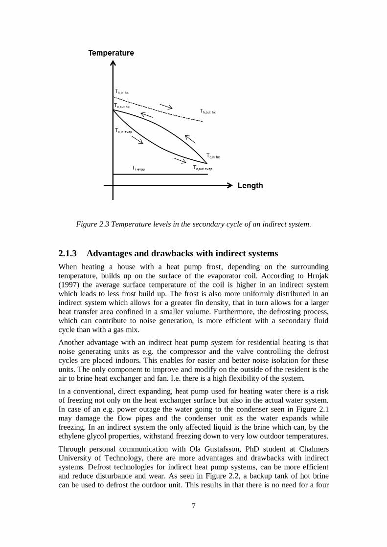
Figure ‎2.3 Temperature levels in the secondary cycle of an indirect system.

2.1.3 Advantages and drawbacks with indirect systems

When heating a house with a heat pump frost, depending on the surrounding

temperature, builds up on the surface of the evaporator coil. According to Hrnjak

(1997) the average surface temperature of the coil is higher in an indirect system

which leads to less frost build up. The frost is also more uniformly distributed in an

indirect system which allows for a greater fin density, that in turn allows for a larger

heat transfer area confined in a smaller volume. Furthermore, the defrosting process,

which can contribute to noise generation, is more efficient with a secondary fluid

cycle than with a gas mix.

Another advantage with an indirect heat pump system for residential heating is that

noise generating units as e.g. the compressor and the valve controlling the defrost

cycles are placed indoors. This enables for easier and better noise isolation for these

units. The only component to improve and modify on the outside of the resident is the

air to brine heat exchanger and fan. I.e. there is a high flexibility of the system.

In a conventional, direct expanding, heat pump used for heating water there is a risk

of freezing not only on the heat exchanger surface but also in the actual water system.

In case of an e.g. power outage the water going to the condenser seen in Figure 2.1

may damage the flow pipes and the condenser unit as the water expands while

freezing. In an indirect system the only affected liquid is the brine which can, by the

ethylene glycol properties, withstand freezing down to very low outdoor temperatures.

Through personal communication with Ola Gustafsson, PhD student at Chalmers

University of Technology, there are more advantages and drawbacks with indirect

systems. Defrost technologies for indirect heat pump systems, can be more efficient

and reduce disturbance and wear. As seen in Figure 2.2, a backup tank of hot brine

can be used to defrost the outdoor unit. This results in that there is no need for a four

8

way valve to reverse the flow, which reduce chances for leakage as well as noise

generation when the valve is operating.

However, there are some drawbacks with indirect systems. As seen Figure 2.2, there

is a need for an extra heat exchanger between the brine and water, which will lead to

temperature losses. This may also result in a higher total system cost. Furthermore, an

extra circulation pump is needed for the brine cycle.

2.2 Sound

The motion or vibration of an object creates small pressure variations in the air around

the static pressure of 105 Pa, which, if large enough, the human ear perceives as

sound. Sound levels are usually measured using the decibel scale, which is a

logarithmic measure expressing the ratio of two sound pressures, intensities or

powers.

Two different sounds at the same sound level are perceived differently, in terms of

loudness, if the frequencies of the sounds are not the same. Loudness is a measure of

the subjective impression of the magnitude of a sound. To measure loudness, an A-

weighted filter is normally used so that the sound frequency is taken into account. The

unit dBA indicates that such a filter is used, and although the correlation between

dBA and loudness is approximate, the A-weighted level has become universally

accepted as the simplest way of measuring noise that does give some correlation with

human response. A 10 dBA increase is perceived as a doubling in loudness due to the

logarithmic nature of the decibel scale. Smith (2011)

2.3 Noise generation in indirect heat pumps

In an indirect air-source heat pump system, the unit placed outdoors contains only a

fan and a heat exchanger. Since this study concentrates solely on the noise generated

outdoors, this subchapter describes which factors that cause the noise generated by

such a unit, and how the noise level can be estimated.

The fan and the heat exchanger together generate noise. The purpose of using a fan is

to generate a flow of air passing through the heat exchanger, creating forced

convection, and thus increasing the heat transfer rate between the fluid and the air.

This air flow through the heat exchanger induces an aero dynamical noise, in this case

called direct noise, which depends on the heat exchanger design and the air velocity.

There is also noise that is generated by the fan itself, which then can be called indirect

noise. Preliminary unpublished studies made by SP Swedish Technical Research

Institute have shown that when trying to reduce the overall noise level in a case like

this, the reduction of the direct noise is much less of an issue compared to the

reduction of the indirect noise generated by the fan.

The noise generation of a fan is dependent on the fan type, its design and the

operating conditions. It is difficult to predict the noise level generated by a fan and the

uncertainties are often large. A general rule is that a fan is quietest at its peak

efficiency point. Performance curves of fans are often results of actual tests and can

be used to find the peak efficiency point of a fan. According to ASHRAE (2009)

Handbook, a simplified expression of the sound power level of a fan can be described

using equation ( 2.1), with which the influence of the heat exchanger on the indirect

9

noise level can be evaluated. It shows that the sound power level depends on the fan’s

own specific sound power level , the air flow rate , the pressure , the blade

frequency increment and the efficiency correction . ASHRAE (2009)

(‎2.1)

Equation ( 2.1) provides the sound power level measured in dB, which is an

inadequate indicator of how the sound is actually perceived by humans. In order to

create an idea of how the noise is perceived, an A-weighted sound power level can be

used, measured in dBA. One way of determining the A-weighted sound power level

of an operating fan is to use its performance curve in which the fan manufacturer

often has entered results from real sound measurements. The disadvantage of using

this method is that it requires studying each particular case manually, which may

become far too cumbersome and time consuming if many cases are to be compared.

Also, the operating condition for which the fan manufacturer has performed sound

measurements may very well not coincide closely enough with the operating

conditions for which the sound power level is to be estimated in other cases. Another

much less cumbersome method to use, if numerous cases need to be compared, is to

theoretically apply an A-filter to the sound power level calculated using equation

( 2.1), thus providing a theoretical A-weighted sound power level. How to apply such

filter is described in ASHRAE (2009), behind which the idea is that the perceived

sound power level depends on the sound frequency. Table 2.1 shows how the filter is

applied.

Table ‎2.1 A-filter appliance for the different octave bands.

Octave band [Hz] 63 125 250 500 1000 2000 4000 8000

[dB] 51 48 49 47 45 45 43 31

[dB]

[dB]

[dB] 5 0 0 0 0 0 0 0

[dB] 0 0 0 0 0 0 0 0

A-filter [dB] -26.2 -16.1 -8.6 -3.2 0 1.2 1 -1.1

As can be read from Table 2.1, the noise is first divided into octave bands, i.e. eight

different frequency intervals. Now, each octave band is assigned its own sound power

level by using equation ( 2.1). The values of are taken from ASHRAE (2009)

Handbook, where there are nominal values for axial propeller fans available. The

efficiency correction is assumed to be equal to zero for each case and each octave

band, thus also making the assumption that the fan being used is operating at peak

efficiency. The A-filter is applied by adding the number of dB given in ASHRAE

(2009) in each octave band. Then, the total sound power levels of all octave band are

summed up, from which a single value is determined which describes the total A-

weighted sound power level.

10

The values of in Table 2.1 are taken from ASHRAE (2009), but in this study they

are slightly altered based on unpublished laboratory measurements made by SP

Swedish Technical Research Institute. The somewhat different values that instead

were used were derived from measurements of noise levels of fans in the same size

and working range as fans in normal heat pumps. The simple reason for doing so is an

attempt to acquire more accurate results. The new values are applied consistently in

the study, meaning that using these values makes no difference when comparing case

to case.

2.4 Psychrometrics

In calculations that in some way treat temperature change of air, consideration needs

to be taken to air humidity. For instance, if the air is humid and its temperature

decreases by passing through a heat exchanger, a portion of the heat transferred to the

cold stream is latent and a portion is sensible. The latent portion is heat contained in

the moisture in the air and will not be included if considering a change in dry bulb

temperature only and a constant value of specific heat. Outdoor air in this study is

considered humid, consideration therefore needs to be taken to both latent and

sensible heat in order to obtain the correct heat transfer.

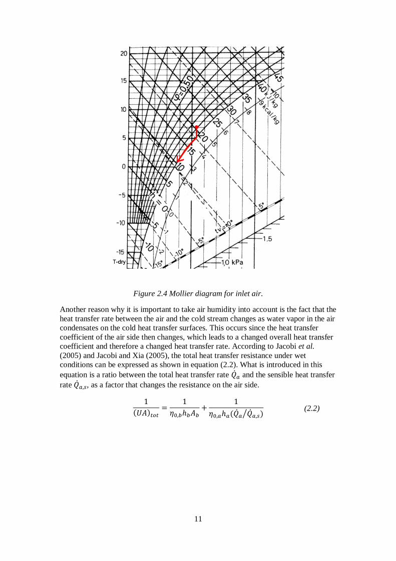
According to the standard testing conditions of air source heat pumps, described in

Swedish Standards Institute (2011), the inlet air should have a wet bulb temperature

of 6˚C if the dry bulb temperature is 7˚C. Given the two conditions, i.e. wet and dry

bulb temperature, a complete knowledge of the state of the air can be obtained by

using for example a Mollier diagram valid for atmospheric pressure. In the Mollier

diagram in Figure 2.4, the state of the air when the inlet temperature is 7˚C is

indicated with a dot. In this study it is assumed that, as the air is cooled, the state

changes along the arrow in the figure. The arrow first points vertically down to the

saturation line where the relative humidity is 100%, and then follows the saturation

line until the cooling stops. This means that the relative humidity of the air gradually

increases until the temperature reaches the dew point, where after the humidity stays

constant at 100% during the rest of the temperature decrease. The change in enthalpy

between the inlet and outlet state, which can be observed using the Mollier diagram,

will then include both latent and sensible heat, and can hence be used to determine the

total heat transferred from the air to the fluid.

11

Figure ‎2.4 Mollier diagram for inlet air.

Another reason why it is important to take air humidity into account is the fact that the

heat transfer rate between the air and the cold stream changes as water vapor in the air

condensates on the cold heat transfer surfaces. This occurs since the heat transfer

coefficient of the air side then changes, which leads to a changed overall heat transfer

coefficient and therefore a changed heat transfer rate. According to Jacobi et al.

(2005) and Jacobi and Xia (2005), the total heat transfer resistance under wet

conditions can be expressed as shown in equation ( 2.2). What is introduced in this

equation is a ratio between the total heat transfer rate and the sensible heat transfer

rate , as a factor that changes the resistance on the air side.

( )

( )⁄ (‎2.2)

13

3 Operating conditions and constraints

In order to find a suitable heat exchanger design, its operating conditions and a set of

constraints must first be determined. A very important constraint is obviously which

level of noise that is considered acceptable, and another is how large (length, height

and width) the heat exchanger is allowed to be. It is also important to determine at

which conditions the heat exchanger is operating, for example what the outdoor air

temperature is. This chapter presents, explains and motivates all the different

constraints and operating conditions that will be used when designing a suitable heat

exchanger.

3.1 Level of noise

According to heat pump test results issued by the Swedish Energy Agency (a), the

level of noise of 14 different air to water heat pumps, tested between 2010 and 2013,

varies between 71 and 56 dBA. Since a purpose of this study is to find a design of a

heat exchanger that allows for a low level of noise, the value of the noise level is

aimed to be 56 dBA or lower. This is a soft target that should be held as low as

possible so that it at the same time allows for a well overall performing system.

3.2 Outdoor air

The state of the outdoor air to be used in this study is set using the Swedish Standards

Institute (2011) paper SS-EN 14511-2:2011 Table 12 - Air-to-water and air-to-brine

units – Heating mode (Low temperatures). The outdoor air condition used in this

study is the first point in the table, stating that the inlet dry bulb temperature is 7 º C,

the wet bulb temperature is 6 ºC, and the relative humidity is 86.66%. The reason for

using this condition is that it is commonly used in standardized heat pump testing.

More air conditions can be used, but only the one mentioned is considered in this

study.

3.3 Brine properties

Just as it is necessary to decide at which outdoor air temperature the heat exchanger

should operate, it is necessary to determine the temperature of the cold stream, i.e. the

brine. The temperature difference between the hot and cold stream in a heat exchanger

is a driving force for heat transfer, which is why the choice of temperature levels is of

such importance. The state of the air at the inlet of the heat exchanger is accurately

described by standards for testing heat pumps, however the state of the brine is not.

Nevertheless, given the outdoor air temperature, and by making assumptions

regarding e.g. minimum temperature differences in the heat exchangers in a reference

heat pump running at these conditions, an estimate of expected brine temperature

levels can be derived.

In order to estimate the brine temperature in an indirect heat pump, an approximate

evaporation temperature of the refrigerant in a direct heat pump is first found.

This is done partly by assuming that the minimum temperature difference

between the streams is 5 K, and that the outlet air temperature is roughly 2.2 ˚C

14

as the inlet air temperature is 7.0 ˚C. The assumption regarding minimum temperature difference is made after consulting Fredrik Karlsson, (researcher at SP)

and the air temperatures are assumed after having reviewed SP test measurements of a

heat pump comparable to the reference heat pump of this study. A third assumption

made is that the temperature of the refrigerant stream is constant, i.e. .

These assumptions lead to the conclusion that the evaporation temperature of the

refrigerant is approximately -2.8 ˚C, as shown in Figure 3.1, as the inlet air

temperature is 7.0 ˚C. For the efficiency of an indirect version of the direct reference

heat pump, it is now assumed that the evaporation temperature of the refrigerant is to

be the same in both types of heat pumps while running at identical conditions. The

additional heat exchanger needed between refrigerant and brine in the indirect version

has a minimum temperature difference of about 2 K, which again is an assumption

made after consulting Fredrik Karlsson about what can be expected from a fluid-to-

fluid heat exchanger in a heat pump.

Finally, the inlet brine temperature , as the outdoor air temperature is 7.0 ˚C, can be approximated to -0.8 ˚C as shown in Figure 3.2.

Figure ‎3.1 Figure describing inlet brine temperature for the reference heat pump.

Figure ‎3.2 Figure describing inlet brine temperature for an indirect heat pump.

In this study, the brine solution is assumed to sustain freezing down to -32 C in

accordance with manufactured heat pumps for the Scandinavian market. In order to do

so, the solution is assumed to be 50:50 % (by volume) water to ethylene glycol

(MEGlobal, 2013). Data for the brine is taken from ASHRAE (2009).

15

3.4 Air flow

The air flow over a conventional heat exchanger for heating of residential buildings in

the size of approximately 6-10 kW is about 2000 – 3500 m3/h. (IVT, 2013) (Thermia,

2010) (Nibe, 2013) Theses direct heat pump systems often have a plate and tube

design of the evaporator. Due to the intention of the study to test different designs, the

value of the air flow is not constrained.

3.5 Fluid flow rate

According to E. Granryd (2007), the flow rate of the secondary loop fluid in an

indirect system can be chosen rather freely. Larger brine flow rate results in a reduced

temperature difference but acquires a higher work input for the pumping system and

therefore reducing the total energy efficiency. Accordantly there are two system

optima in a heat pump due the flow rate of the system. One giving maximum energy

capacity and one resulting in minimum total energy input demand. However,

changing the flow rate, and thereby the velocity in an already manufactured heat

exchanger may result in a change from turbulent to laminar flow or vice versa. This

can cause a major drop in the heat transfer capability if the heat exchanger is not

designed for this new condition. In this study, a fluid mass flow rate of 1 kg/s will be

tested and evaluated.

3.6 Fluid temperatures

The heat exchanger is investigated under heating mode while the inlet and outlet

temperature of the water (at the heat pump condenser) is 30 ºC and 35 ºC respectively.

This follows the SS-EN 14511-2:2011 standard for low temperatures. (Swedish

Standards Institute 2011)

3.7 Dimensions

The permitted size of the outdoor unit is a difficult constraint to set since there are no

standards or regulations as to how large it may be. Therefore, the dimensions of the

outdoor unit of the heat pump with the lowest level of noise according to

measurements made by the Swedish Energy Agency (a), the IVT Premium Line A

Plus, are used as reference. This unit has a height of 152 cm, a width of 96 cm, and a

depth of 115 cm. The heat pump with the smallest outdoor unit, but not lowest noise

level, is the Invest Living LVE-09. This outdoor unit is also used for comparison and

has a height of 70 cm, a width of 84 cm, and a depth of 32 cm.

The dimensions of the reference units do not have to be exactly matched, they are

used mostly for the sake of comparison. If this study results in that the chosen heat

exchanger and fan allow the outdoor unit of an indirect heat pump to be smaller, then

that is considered an advantage. Hence, the dimensions of the outdoor unit are quite

free to vary. An indirect constraining factor for the heat exchanger size, and thereby

also the outdoor unit, may be that the fan must be large enough to supply enough

surface of the heat exchanger with an air flow. For instance, a very small fan, in

relation to the heat exchanger, would create an uneven airflow across the heat

16

exchanger heat transfer surface. For that reason, the necessary fan size may become

an indirect constraint for the size of the outdoor unit.

3.8 Heat load

Between the year 2010 and 2013, 14 different heat pumps for residential heating were

tested by the Swedish Energy Agency (a). The heat output, as the outdoor temperature

was 7 ºC and the water temperature output was 35 ºC, varied between 7.6 - 11.2 kW.

The unit with the lowest noise level according to the tests, IVT Premium Line A Plus,

has an output of 9.4 at the air temperature of 7 ºC, which are set as the desired output

value of the condenser unit in this study. The COP-value at this point is 3.9.

3.9 Pump work

As an indirect system consists of an additional fluid pump, (seen in figure 2.2) to feed

the heat exchanger that exchanges heat between the brine and the refrigerant, the

pump work need to be kept as low as possible. If the pump work is too high, the

overall efficiency of the heat pump will suffer. After consulting Caroline Haglund

Stignor, the pump work was set to not exceed 100 W, as a level of limitation. The

efficiency of the circulation pump is set to 25 % in accordance with the best

preforming pump in the test carried out by the Swedish Energy Agency (b).

17

4 Heat exchanger types to be analyzed

Compact heat exchangers are commonly used to transfer heat between gas-to-gas and

gas-to-liquid, and cover many different applications such as residential heating,

refrigeration, food showcase and process industries. This study is regards heat transfer

between liquid and gas. Two types of compact heat exchangers will be evaluated, one

type with round tubes and continuous fins, and one with flat tubes and continuous

fins.

The most common exchanger surface for modern residential heat pumps is the round

tube with continuous fins, which can be seen in Figure 4.1. All of the heat pumps in

the tests carried out by the Swedish Energy Agency (a) where configured in this way.

Compared to a bare tube bank, this conventional design with circular tubes and

continuous fins increases the heat transfer area. This is because the fins enable a

second and larger heat transfer area. This is desirable in gas-to-liquid heat transfer

applications as an optimum design tends to demand maximum heat transfer area

according to Kays & London (1984).

Figure ‎4.1 Schematics of a round tube heat exchanger design, d is the diameter for

the tubes, Tpl is the longitudinal tube pitch and Tpt specifies the transversal tube pitch.

The second evaluated heat exchanger type is the one with flat tube with continuous

fins, seen in Figure 4.2. The tubes in these heat exchangers, in this study, are

staggered.

18

Figure ‎4.2 Schematics of a flat tube heat exchanger design.

One of the flat tube heat exchanger modeled in this study is equipped with wavy fins.

The difference between wavy and plain fins is simply the wavy geometry which is

intended to allow for a better mixture of the air and thus better heat transfer

conditions.

Both heat exchanger types have a large number of fins, densely grouped together in

order to increase the heat transfer area. The horizontal distance between the fins is

called fin pitch and often given in number of fins per meter. The fin pitch is,

especially in Nordic climate, an important parameter due to the risk of frost build up

on the surface. As frost builds up on the heat exchanger surface, the heat transfer rate

decreases. A small fin pitch will result in more frequent defrost cycles due to the fact

that the air flow passage gets clogged more easily. The fin pitch of the evaluated

round tube heat exchangers in this study is in line with the units manufactured for the

Nordic market. The most common fin material for the residential heat pumps is

aluminum. Dimensions for the modelled heat exchangers are seen in Appendix 1.

Another parameter is the number of passes that a heat exchangers has. It is simply

how many times the fluid inside the tubes passes the heat exchanger coil. Figure 4.3

shows a heat exchanger seen from above, when the number of passes is four. As seen

in the figure, the number of passes would be four as the fluid enters in the first row,

turns in the u-bends, comes back in the second row, goes back into the third and

finally exit into the fourth row. I.e. the number of passes in this study is equivalent

with how many rows deep the heat exchanger is.

19

Figure ‎4.3 Description of the concept of passes.

When referring to the number of circuits that any of the heat exchangers included in

this study has, it basically describes the ratio between the number of rows that the heat

exchanger is high, and the number of fluid inlets the unit has. For instance, if the heat

exchanger has a fluid inlet on each row, the number of circuits is one. The number of

circuits is increased by feeding the fluid to fewer inlets, for example to only half as

many, thus forcing the fluid that enters an inlet to flow a longer distance. Figure 4.4

shows three examples where the number of circuits is one, two and three. The crossed

circles represent tubes at which the fluid enters the heat exchanger. The fluid enters at

an inlet and then always flows through all passes (see Figure 4.4). If the number of

circuits is one, the fluid exits at the outlet after only four passes. If the number of

circuits instead is more than one, the fluid will enter a new inlet after having exited at

the outlet of the fourth pass.

Usually in heat exchangers with round tubes, a simple U-shaped bend is used to

connect the passes to each other. In heat exchangers with flat tubes, the way the

passes are connected is not as simple. Instead, manifolds are mounted on the sides of

the heat exchanger, into which the fluid enters and then is distributed back to all tubes.

Using the heat exchanger in Figure 4.4 with three circuits as an example, the fluid

would flow through four passes (since the unit four rows deep) and three rows,

meaning a distance three times as long as the fluid would flow if the number of

circuits instead were only one. A reason why this this is done is that if the mass flow

is kept constant, increasing the number of circuits will force the fluid to flow faster,

thus affecting the heat transfer capacity on the fluid side. Having fewer inlets may

also be preferable from a manufacturing point of view, although this is neglected in

this study.

20

Figure ‎4.4 Schematic illustration of heat exchangers with different number of circuits.

21

5 Theory behind modelling of designs

In order to calculate the heat transfer rate and pressure drop in a heat exchanger

of a given type, geometry, flow rates and entry temperatures, and a number of steps

are required. Using the P-NTU method, the heat transfer rate depends on the

temperature effectiveness and of the heat exchanger according to equation ( 5.1)

(‎5.1)

where and is the heat capacity rate for the two fluids exchanging heat such as

. is the maximum temperature difference, i.e. | |.

The temperature effectiveness is given in equation ( 5.2) from Shah and Sekulić

(2003)

[

]

[

]

(‎5.2)

where n is the number of passes, is the heat capacity ratio and is the thermal

effectiveness of each pass. The temperature effectiveness depends of the actual flow

arrangement of the heat exchanger. In this study, all heat exchangers evaluated are of

a cross-flow type and the numbers of passes are to be seen as identical in flow

arrangement with identical individual NTU, which is further explained below.

The thermal effectiveness of each pass, is given by

(‎5.3)

else

(‎5.4)

with the definition of

(‎5.5)

else

(‎5.6)

and

(‎5.7)

else

(‎5.8)

22

The heat capacity rate R1 is simply given by

(‎5.9)

introduced in equation ( 5.10) is the heat exchanger effectiveness from Incropera

and DeWitt (2007)

[(

) ( )

{ ( ) }

] (‎5.10)

where is the number of transfer units. Equation ( 5.10) is valid for cross-flow,

single pass and with both fluid unmixed. The fluid inside the tubes in a multiple-tube-

row cross-flow exchanger is considered mixed at any cross section. However

according to Shah and Seculic (2003) the fluid can be considered as unmixed as it is

split and distributed between the tube rows. In practice a number of passes around

four will give an unmixed characteristic. With less than four or five passes the fluid is

partially unmixed or partially mixed. Because of the difficulties in interpreting exactly

when Equation (5.10) is valid, it assumed to be valid for all number of passes in the

range 2-12.

The number of transfer units, , used in the equation ( 5.10) is given by Shah and

Sekulic (2003) as

(‎5.11)

where is the overall heat transfer coefficient. To determine the heat transfer area the

surface area of all tubes and fins are calculated. The -value is determined using

equation ( 5.12) from Kays and London (1984)

( ) ⁄

(

)

(‎5.12)

where the middle term, which represents the resistance for heat transfer through the

tube wall, is neglected due to its very small contribution to the total resistance.

and represent the overall surface effectiveness on the hot air and cold brine side

respectively, and is the heat transfer coefficients.

is the local sensible heat

ratio.

As the brine side does not have any extended surface, is set to one. Equation

( 5.12) is therefore reduced to

23

(

)

(‎5.13)

The overall surface effectiveness on the air side , needs to be weighted. This is

because the temperature gradient within the fins extending into the fluid is reducing

the surface effectiveness. The surface effectiveness for the hot air side is given by the

equation below form Kays and London.

( ) (‎5.14)

Where is the fin efficiency given by equation ( 5.15)

( )

(‎5.15)

is defined as half the wall spacing between the tubes, and m is given by

√

(‎5.16)

for thin sheets fins. is the thermal conductivity of the fin material.

In accordance with Jacobi and Xia (2005) the local sensible heat ratio variation,

correctly expressed as , is assumed to vary negligibly over the surface area

and therefore equal to .

The air heat transfer coefficient is given by Kakaç, Liu and Pramuanjaroenkij (2012)

as

( )

(‎5.17)

where is the specific heat capacity for air and is the Prandtl’s number which

is linear interpolated within the operating temperature range for the air side. is the

Colburn correction factor.

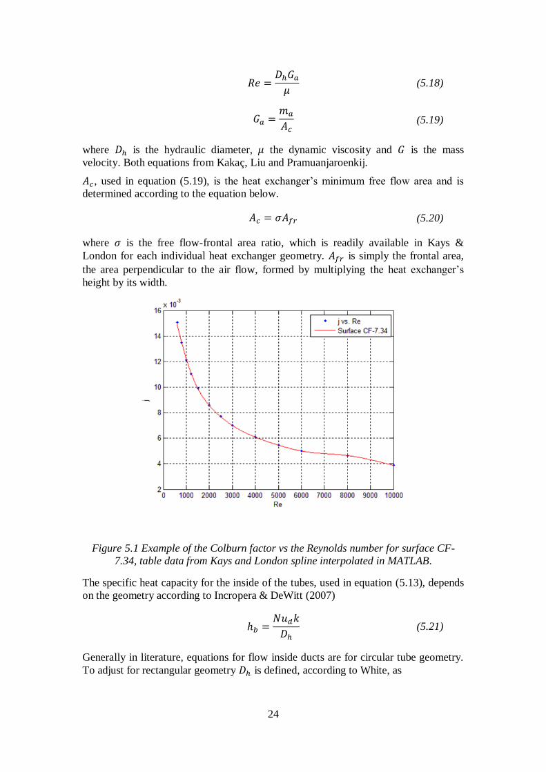
The Colburn correction factor is given by data from Kays & London. For the heat

exchangers with flat tubes with continuous fins table data from Kays & London where

curve fitted through piecewise polynomial interpolation, so called spline, to get a

small interpolation error in MATLAB. An example of this is to be seen in Figure 5.1.

Graphical data for round tube with continuous fins where extracted by hand from

figure 10.91 and 10.92 in Kays & London and again spline interpolated. This will give

a somewhat larger error compared to table data, but is assumed to not affect the

results noticeably. The Colburn factor is basically a modified Stanton number that

account for variations in the fluids Prandtl number.

From the interpolated data, the j factor is a function of the Reynolds number on the air

side.

24

(‎5.18)

(‎5.19)

where is the hydraulic diameter, the dynamic viscosity and is the mass

velocity. Both equations from Kakaç, Liu and Pramuanjaroenkij.

, used in equation ( 5.19), is the heat exchanger’s minimum free flow area and is

determined according to the equation below.

(‎5.20)

where is the free flow-frontal area ratio, which is readily available in Kays &

London for each individual heat exchanger geometry. is simply the frontal area,

the area perpendicular to the air flow, formed by multiplying the heat exchanger’s

height by its width.

Figure ‎5.1 Example of the Colburn factor vs the Reynolds number for surface CF-

7.34, table data from Kays and London spline interpolated in MATLAB.

The specific heat capacity for the inside of the tubes, used in equation ( 5.13), depends

on the geometry according to Incropera & DeWitt (2007)

(‎5.21)

Generally in literature, equations for flow inside ducts are for circular tube geometry.

To adjust for rectangular geometry is defined, according to White, as

25

(‎5.22)

where Ƥ is the wetted perimeter. This enables for the use of the same equations for the

rectangular as with circular geometry.

The Nusselt number for laminar flow conditions inside the round tubes is taken from

Gnielinski (1989) as

(

( ( ) )

) (‎5.23)

where is defined by the equation below

(‎5.24)

For turbulent flow conditions the Nusselt number inside the round tubes can be taken

from two different correlations, Gnielinski (1989) and Dittus-Boelter.

The Gnielinski correlation

( ) ( )

√( ) (

)

(‎5.25)

with equal to

( ) (‎5.26)

which is valid for .

The Dittus-Boelter correlation, quoted by Haglund Stignor (2009), is equal to

( ) ( )

(‎5.27)

Gnielinski’s equation for Nusselt numbers for laminar flow is valid only for . For , equation ( 5.27) and ( 5.25) are found possible to use. In

order to help make a decision on what to assume for the interval not covered by either

equation, the equations are plotted for a range of Reynolds numbers. The curves for

equation ( 5.23) and ( 5.25) intersect close to , relatively close to where the

equation for laminar flow stops being valid, which can be seen in Figure 5.2. From the

intersection of the curves and up, the curve for equation ( 5.25)is approximately linear.

Hence, in order to avoid a sudden change in Nusselt number, it is therefore assumed

that equation ( 5.23) is valid and equation ( 5.25) is valid for . Equation (5.27) is not used since it does not intersect as well with ( 5.23)where

( 5.23) stops being valid.

26

Figure ‎5.2 Nusselt vs. Reynolds number for Gnielinski's turbulent and laminar

correlation.

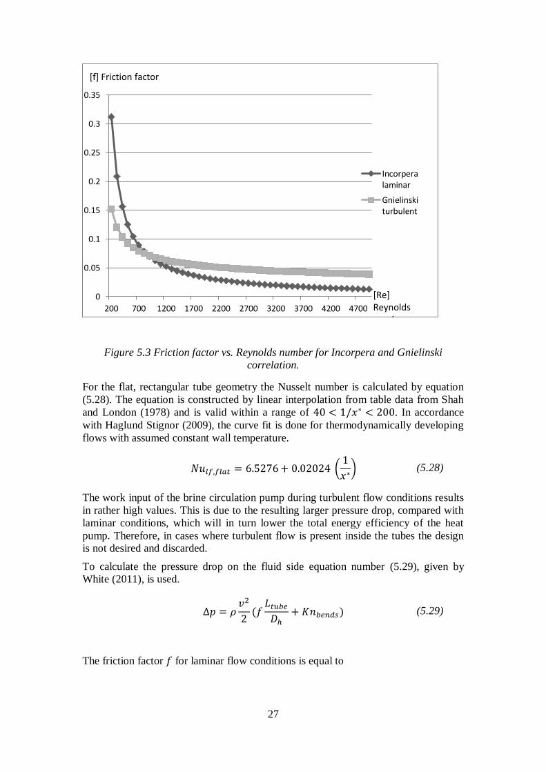
When calculating the liquid side pressure drop for laminar flow, the friction factor

is determined using equation ( 5.30) according to Incorpera. According to Gnielinski

(1989), equation ( 5.26) is to be used to calculate for turbulent flow, and is valid for

. In order to avoid a sudden change in friction factor value, and to make

consistent assumptions, it is assumed that the equation for laminar flow is valid for

. In this case, there is no intersection at this point, why a perfectly linear

equation is established stretching from the point where equation ( 5.30) stops being

valid to where equation ( 5.26) starts being valid, i.e. at . For ,

the equation for turbulent flow is used. Both equations are plotted for a range of

Reynolds numbers in Figure 5.3.

-80

-60

-40

-20

0

20

40

60

80

100

0 500 1000 1500 2000 2500 3000 3500 4000 4500

Gnielinskilaminar

Gnielinskiturbulent

[Nu] Nusselt

[Re] Reynold

27

Figure ‎5.3 Friction factor vs. Reynolds number for Incorpera and Gnielinski

correlation.

For the flat, rectangular tube geometry the Nusselt number is calculated by equation

( 5.28). The equation is constructed by linear interpolation from table data from Shah

and London (1978) and is valid within a range of . In accordance

with Haglund Stignor (2009), the curve fit is done for thermodynamically developing

flows with assumed constant wall temperature.

(

) (‎5.28)

The work input of the brine circulation pump during turbulent flow conditions results

in rather high values. This is due to the resulting larger pressure drop, compared with

laminar conditions, which will in turn lower the total energy efficiency of the heat

pump. Therefore, in cases where turbulent flow is present inside the tubes the design

is not desired and discarded.

To calculate the pressure drop on the fluid side equation number ( 5.29), given by

White (2011), is used.

(

) (‎5.29)

The friction factor for laminar flow conditions is equal to

0

0.05

0.1

0.15

0.2

0.25

0.3

0.35

200 700 1200 1700 2200 2700 3200 3700 4200 4700

Incorperalaminar

Gnielinskiturbulent

[f] Friction factor

[Re] Reynolds number

28

(‎5.30)

which is valid in the range for single phase flow, circular tube, and a Reynolds

number of .

For turbulent flow conditions i.e. equation ( 5.26) is valid.

The coefficient describes resistance from different shapes such as e.g. valves,

elbows and tees. It is often, in literature, correlated to the raw size of the pipe and not

with the Reynold numbers or roughness of the surface. Furthermore the value of is

often provided from different manufactures in the literature, and reported for turbulent

flow conditions. Different forge and molding techniques give somehow different loss

coefficients and can therefore vary quite much for the same tube diameter. With this

in mind, the uncertainty of the value is rather high. (White)

Because of the uncertainties, the same value is used for both types of heat

exchangers.

In accordance with Haglund Stignor (2002) the -value is set to 2.28 and multiplied

with the numbers of bends, .

Finally, to determine the air side pressure drop between the inlet and the outlet,

equation ( 5.31) is used from Kakaç, Liu and Pramuanjaroenkij (2012).

(

( ) (

)) (‎5.31)

and represent air density at the inlet and outlet respectively. is the friction

factor.

is correlated according to

(‎5.32)

is the air flow length, i.e. the depth of the core.

( ) (‎5.33)

The friction factor is, as with the Colburn factor, extracted by using spline

interpolation from table data for flat tubes with continuous fins. Again, graphical data

were extracted by hand from the upper curves in figure 10-91 and 10-92 in Kays and

London (1984).

29

6 Calculation method

All equations and correlations regarding for example heat transfer rate and noise

levels, needed to determine the necessary size of a heat exchanger of a specific type,

was presented in the previous chapter. What follows here is a description of the

approach taken to determine a necessary heat exchanger size, explaining the way

constraints, such as noise level and heat transfer rate, are taken into account.

The computer software Matlab was used as a tool to perform all necessary

calculations and generate desirable results. The reason why Matlab was identified as a

suitable tool is that it makes possible using the method of trial and error in a time

efficient manner. The first step in the Matlab script design was naturally to enter all

relevant equations and data for the type of heat exchanger to be evaluated. Secondly,

it was selected which dimension of the heat exchanger to vary, i.e. either its frontal

area or depth. At this point, the program first assumed a specific frontal area and a

specific air flow. Knowing the exact geometry of the unit and the air flow, the heat

transfer rate could be determined using the different correlations. In case it turned out

that the resulting heat transfer rate was below the constraint, the air flow was

increased by another ten m3/h. Using this increased air flow, and if the heat transfer

rate again turned out to be below the constraint, another ten m3/h was added, and so

on, until the sufficient heat transfer rate finally was reached. By this time, the

necessary air flow had been determined for one specific frontal area of one specific

heat exchanger type. Given the air flow and the resulting pressure drop, the noise

level could be calculated.

The next step was to increase the frontal area, and repeat the same procedure as before

to determine the necessary air flow and resulting noise level for the heat exchanger of

slight larger size. As the targeted noise level was reached, the size increase would

stop. At all times when varying the frontal area, both height and width were varied

equally, meaning that a quadratic frontal area always was formed as can be seen in

Figure 6.1. When varying the frontal area, the depth was held constant. Similarly, the

frontal area was kept constant when the impact of a change in depth was studied. The

same Matlab script, with only minor modifications, was applied for all heat exchanger

types and for when the depth was varied instead of the frontal area.

30

Figure ‎6.1 Stepwise increase in frontal area.

31

7 Modelling results and parameter evaluations

After having modelled all four heat exchangers, results have been acquired that

indicate the difference in suitability between them. This chapter first presents a

comparison of all heat exchangers, with the purpose to highlight which single one that

is superior to all others, letting small volume be the deciding factor. As previously

explained, small volume is assumed to be related to low cost. The results are then

analyzed and explained by comparing the different types, and finally an evaluation of

parameters is made. The evaluation is made regarding only the best performing heat

exchanger in order to attempt to further optimize its design.

7.1 Heat exchanger ranking

When determining which one of the four different modeled heat exchangers that is

considered to be the best, the noise level and heat output requirements were set to

equal values in all cases. More specifically, as a heat output of 7 kW was fulfilled by a

heat exchanger, while causing no more or less than a noise level of 56 dBA, the

necessary heat exchanger volume was noted. The methodology to reach this result is

more accurately described in chapter 6.

When ranking the heat exchangers, the depth of each one is four rows, while the width

and height are equal so that the frontal area is quadratic. The reason why a depth of

four rows was chosen is that it is a common feature of heat exchangers in heat pumps.

Figure 7.1 shows the necessary volumes of the different heat exchangers for when

they all reached the same targeted noise level as well as heat output. In order to

abbreviate the descriptions of the heat exchangers, the flat tube plain fin heat

exchanger is called FFT1, the flat tube wavy fin is called FFT2, the round tube with

the smaller tube diameter is called FCT1 and the fourth is called FCT2. It can be seen

that FFT1 is the smallest, and for that reason, FFT1 is also presumably also the

cheapest.

It is however not by much that FFT1 defeats FFT2. In fact, the difference in necessary

volume between the two is so small that it may even be negligible. Why a difference

can be seen at all is described later in this chapter. If now studying the two round tube

heat exchangers in Figure 7.1, it is obvious that both need to be considerably larger

than any of the flat tube heat exchangers. The necessary volume of FCT1 is even

about twice that of FFT1, while FCT2 in turn needs to be about three times larger in

volume than FCT1. It should be noted that the depth measured in millimeters is not

the same for all heat exchangers, i.e. it is not only the frontal area that differs between

them. It is true all heat exchangers are four rows deep, but since their tube geometries

differ, their depths differ as well. All measurements, including the differences in

depth, can be seen in Table 7.1. The reason why the numbers presented in the figure

are that precise is that they are measurements directly based on number of rows. In a

way, the calculations cannot be considered accurate enough to determine necessary

height, width, and depth that exactly.

32

Figure ‎7.1 Necessary volume for the heat exchangers modeled.

Table ‎7.1 Result of the modeled heat exchangers that reach the targeted noise level.

Heat exchanger Height [mm] Width [mm] Depth [mm]

Flat tubes - FFT1 701 701 79

Flat tubes - FFT2 729 729 79

Round tubes - FCT1 1102 1102 76

Round tubes - FCT2 1263 1263 151

To summarize the ranking of the four different heat exchangers, FFT1 is decided to be

considered the one that shows signs of being the most preferable one from a noise

perspective. It is very closely followed by FFT2, but since there apparently is some

difference, it is only FFT1 that will be analyzed further in chapter 7.2. Both round

tube heat exchangers show signs of being considerably less preferable than any of the

flat tube heat exchangers, especially FCT2. In depth explanations as to why there are

differences in necessary volume between the heat exchanger types follow next.

0.00

0.05

0.10

0.15

0.20

0.25

0.30

FFT1 FFT2 FCT1 FCT2

m3

33

7.1.1 Discussion - round tube vs. flat tube heat exchangers

When comparing the best performing heat exchanger with round tubes (FCT1) to the

best performing with flat tubes (FFT1), it is evident that FFT1 is superior due to the

fact that it is smaller, while still achieving sufficient heat transfer rate as well as

causing a noise level of no more than 56 dBA. The difference in size is significant

since FCT1 displaces more than twice the volume. The reason why this is the case, i.e.

why FFT1 is more suitable from a noise perspective, partly has to do with the fact that

the heat transfer resistance on the tube side of FFT1 is about half of the resistance on

the tube side of the FCT1, as can be seen in Table 7.2 . If the resistance on the tube

side is low, the resistance on the outside does not need to be lowered as much by a

high air flow, and thus the air pressure drop and noise level do not rise. The most

contributing factor to why the tube side resistance for FFT1 is lower is that the tube

side heat transfer coefficient is more than twice as high. Another contributing factor is

the difference tube side heat transfer area, but Table 7.2 indicates that this difference

is very little. The heat transfer coefficient differs between the two heat exchangers

depending on the Nusselt number and hydraulic diameter of the inside of the tubes.

The Nusselt number differs only little, as can be seen in Table 7.2, but there is a

significant difference in hydraulic diameter. A smaller hydraulic diameter is

preferable to achieve a high heat transfer coefficient, thus the FFT1 has less heat

transfer resistance on the tube side. Intuitively it makes sense that a flat tube has less

resistance on the fluid side since more fluid is in contact with the tube walls than in a

round tube. It may be tempting to draw the conclusion that the tube side heat transfer

resistance for FCT1 can be lowered simply by decreasing the hydraulic diameter its

tubes. However, doing so at the same time decreases the tube side heat transfer area,

which causes the resistance to rise. Therefore, FFT1 has preferable heat transfer

properties on the tube side, leading to less required air flow on the air side, and thus

less noise generation. Nevertheless, it is important to stress the fact that Table 7.2

shows that the pump work on the tube side is significantly larger for FFT1. The pump

work is however still below 100 W, which is assumed to be the level of limitation.

On the air side, there is a difference in heat transfer capacity as well. In fact,

according to Kays and London (1984), the friction factor has a tendency to often be

lower for FCT1. Also, the Colburn factor is often higher for FCT1. These are actually

advantageous properties from a noise perspective, since they are synonymous with

low pressure drop and heat transfer rate resistance. However, since the heat transfer

resistance on the tube side is so much lower for FFT1, the advantageous properties on

the air side that FCT1 possesses do not make big enough of a difference.

34

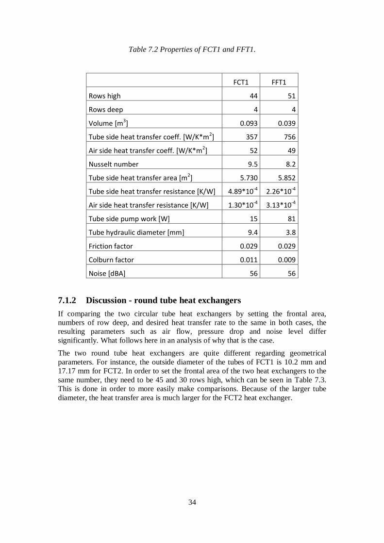
Table ‎7.2 Properties of FCT1 and FFT1.

FCT1 FFT1

Rows high 44 51

Rows deep 4 4

Volume [m3] 0.093 0.039

Tube side heat transfer coeff. [W/K*m2] 357 756

Air side heat transfer coeff. [W/K*m2] 52 49

Nusselt number 9.5 8.2

Tube side heat transfer area [m2] 5.730 5.852

Tube side heat transfer resistance [K/W] 4.89*10-4 2.26*10-4

Air side heat transfer resistance [K/W] 1.30*10-4 3.13*10-4

Tube side pump work [W] 15 81

Tube hydraulic diameter [mm] 9.4 3.8

Friction factor 0.029 0.029

Colburn factor 0.011 0.009

Noise [dBA] 56 56

7.1.2 Discussion - round tube heat exchangers

If comparing the two circular tube heat exchangers by setting the frontal area,

numbers of row deep, and desired heat transfer rate to the same in both cases, the

resulting parameters such as air flow, pressure drop and noise level differ

significantly. What follows here in an analysis of why that is the case.

The two round tube heat exchangers are quite different regarding geometrical

parameters. For instance, the outside diameter of the tubes of FCT1 is 10.2 mm and

17.17 mm for FCT2. In order to set the frontal area of the two heat exchangers to the

same number, they need to be 45 and 30 rows high, which can be seen in Table 7.3.

This is done in order to more easily make comparisons. Because of the larger tube

diameter, the heat transfer area is much larger for the FCT2 heat exchanger.

35

Table ‎7.3 Dimensions for finned circular tubes.

FCT1 FCT2

Tube diameter [m] 0.0102 0.017

Rows high [nr] 45 30

Rows deep [nr] 4 4

Frontal Area [m2] 1.272 1.259

Depth [m] 0.076 0.151

Air flow [m3/h] 6500 9800

The Colburn factor for the FCT2 heat exchanger is smaller at all Reynolds numbers

compared to FCT1 exchanger. This empirical relationship between Reynolds number

and Colburn factor forces the airflow to be higher for the FCT2 heat exchanger in

order to achieve a higher heat transfer coefficient. As the air flow increases, the

Colburn factor declines but at the same time the mass flux increases, and at a stronger

rate which results in a higher heat transfer coefficient.

As with the Colburn factor, the friction factor is lower at all Reynolds number for

FCT2. The corresponding pressure drop for the air is anyhow larger for FCT2 as the

mass flux is considerably larger and in square in the pressure drop equation ( 5.31) ,

seen in chapter 5. As the two round tube heat exchangers have different geometrical

outlines the total depth is not equal at the same row depth. The total depth of FCT2 is

twice as deep as the FCT1, as seen in Table 7.3, due to the fact that the diameter of

the tubes and the tube pitch are larger.

A deeper core increases the pressure drop as the contribution in the equation on the air

side is a factor of four times the core depth divided by the hydraulic diameter, as seen

in equation ( 5.32).

As the FCT2 heat exchanger has a deeper core, the total volume and heat transfer area

is larger compared to FCT1. This is good in the view of heat transfer as the -value

increases but at the cost of a higher pressure drop as stated above. The noise

generation of the fan due to the operating conditions is highly dependent on the

pressure drop as seen in equation ( 2.1), Chapter 2.3. I.e. the larger -value of the

FCT2 is considered good for the heat transfer rate but makes the heat exchanger suffer

a quite large noise penalty.

Another factor that highly contributes to the noise level is the air flow rate. As the

Colburn factor for the FCT2 is lower compared to the FCT1, the air flow needs to be

higher in order to enhance the mass velocity. In the same time, increasing air flow

cause higher Reynolds number that lowers the Colburn factor.

36

7.1.3 Discussion - flat tube heat exchangers

When ranking the four heat exchangers, it was seen that the difference in necessary

volume between the two flat tube heat exchangers was very little, possibly even

negligible. However, a difference did exist and in the reason why is explained here.

The two flat tube heat exchangers calculated in the model only differ in fin geometry

as FFT1 has plain fins while FFT2 has wavy fins. As when comparing the round tube

heat exchangers, the Colburn factor for the two flat heat exchangers differs. FFT2 has

higher Colburn factor value for the corresponding Reynolds value. This inherent

property forces the air flow to be higher for the FFT1 with plain fins, seen in

Table 7.4.

Table ‎7.4 Dimensions for finned flat tubes.

FFT1-(2)

Tube dimensions [m] 0.0187x0.0025

Rows high [nr] 53

Rows deep [nr] 4

Frontal Area [m2] 0.531

Depth [m] 0.079

Air flow [m3/h] 4900 (4700)

A high air flow may intuitively signal that the noise level is higher, both since the

noise level depends directly on the air flow and indirectly through the fact that the

mass velocity Ga, which is a component in the pressure drop equation, is higher.

However, when comparing FFT1 with FFT2 is can be seen that the f-factor is lower

for the plain FFT1. As the friction factor is lower the corresponding pressure drop is

lower for FFT1.

The wavy fins of the FFT2 has the prerequisites for better heat transfer due to the

larger heat transfer area and a larger Colburn factor for the corresponding Reynolds

number. However, the lower f-factor for the FFT1 causing a lower pressure drop

makes the heat exchanger a more preferable choice from a noise perspective.

7.2 Evaluation of design parameters

This chapter has the purpose to quantify and explain the impacts of changes in

different important design parameters such as heat exchanger frontal area, depth,

number of parallel circuits, and fluid mass flow. As previously described, it is the heat

exchanger with flat tubes and plain fins that proved to have preferable properties, why

only this heat exchanger is subject to all analysis in this chapter.

37

Figure 7.2 describes how the noise level depends on the frontal area of the heat

exchanger. It intuitively makes sense that the noise level decreases as the frontal area

increases, since the heat transfer area is increased, so that in turn less forced

convection (i.e. air flow and resulting pressure drop) is needed to generate sufficient

heat transfer rate. Also, as the area increases, the air velocity decreases, which is a

contributing factor to pressure drop and hence also to noise level. The change in pump

work due to the growth in frontal area is negligible.

Figure ‎7.2 Noise level as a function of heat exchanger frontal area.

The number of circuits is increased by feeding the fluid to fewer inlets on the heat

exchanger, thus forcing the fluid that enters an inlet to flow a longer distance as long

as the combined length of all tubes is kept unchanged. For example, when increasing

the number of circuits from one to two, the fluid is fed to half as many inlets and

therefore needs to flow twice the distance. Doing so has several effects on the fluid

dynamics and the heat transfer capacity on the fluid side. As the number of circuits is

increased and the fluid mass flow kept constant, the fluid velocity is forced to rise,

which in turn causes the fluid’s Reynolds number to increase. This causes an increase

in both fluid side pressure drop and Nusselt number. A direct effect of the change in

pressure drop is that more work is required to be done by the fluid side circulation

pump, and the effect of a larger Nusselt number is that the fluid side heat transfer

resistance decreases. For this reason, there is a tradeoff between a high and a low

number of circuits.

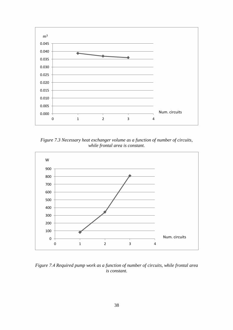
When in Figure 7.3 observing the necessary volume of the flat tube heat exchanger, it

is apparent that less is needed the higher the number of circuits is. The reason why

only one, two and three circuits are tested is the resulting large increase in pump

work, which is presented in Figure 7.4. It is worth noticing that if the number of

circuits is increased from one to two, or from two to three, the necessary heat

exchanger volume is decreased by very little.

0

1000

2000

3000

4000

5000

6000

7000

0

10

20

30

40

50

60

70

0.381 0.398 0.416 0.434 0.453 0.472 0.491 0.511 0.531 0.552 0.573

Noise

Air flowdB

m2

m3/h

38

Figure ‎7.3 Necessary heat exchanger volume as a function of number of circuits,

while frontal area is constant.

Figure ‎7.4 Required pump work as a function of number of circuits, while frontal area

is constant.

0.000

0.005

0.010

0.015

0.020

0.025

0.030

0.035

0.040

0.045

0 1 2 3 4

Num. circuits

m3

0

100

200

300

400

500

600

700

800

900

0 1 2 3 4

Num. circuits

W

39

Figure 7.5 shows, as expected, how the fluid’s Reynolds number grows as the number

of circuits increases. This in turn leads to a higher heat transfer coefficient on the fluid

side.

Figure ‎7.5 Fluid's Reynolds number volume as a function of number of circuits, while

frontal area is constant.

As can be seen in Figure 7.6 where the heat transfer resistances on the fluid side and

air side, as well as their sum are presented, the resistance on the fluid side has a

tendency to be lower than the resistance on the air side. This is the explanation to why

the necessary size does not decrease as significantly for the flat tube heat exchanger,

as the number of circuits is increased. The preferable measure to take is to decrease

the highest resistance, which happens to be the opposite of what occurs in this case.

Increasing the number of circuits does however bring some effect, but at a large

expense of pump work as can be seen in Figure 7.4 above. If assuming that the pump

work should be kept below 100 W, in order for the pump not to be a significant

contributing factor to large energy consumption, the only viable choice is to have one

single circuit.

0

100

200

300

400

500

600

700

800

900

0 0.5 1 1.5 2 2.5 3 3.5

Num. circuits

Re

40

Figure ‎7.6 Heat transfer resistances volume as a function of number of circuits, while

frontal area is constant.

When studying the effects of increasing the depth of the heat exchanger, it becomes

apparent that a minimum in noise generation occurs at a certain depth. This

occurrence is shown in Figure 7.7, which indicates that the noise level is lowest when

the heat exchanger is around six rows deep. The reason why this happens naturally

has to do with air flow and pressure drop. Figure 7.8 shows both the air flow and

pressure drop, while Figure 7.9 shows the heat transfer resistances on both sides of the

heat exchanger. Together, these two figures help explain the occurrence of a

minimum in noise level.

When studying Figure 7.9, it is evident that the resistance on the tube side is

significantly larger than that on the air side when the heat exchanger is only a couple

of rows deep. The resistance on the tube side is high when the depth is low due to the

fact that the tube side area is small. Hence, the air side resistance needs to be much

lower in order for sufficient heat transfer rate to be reached between the streams. This

is achieved by increasing air flow, directly causing a high pressure drop and noise

level. As the tube side heat transfer area increases when increasing depth, the tube

side resistance therefore decreases. Consequently, the air flow is allowed to decrease,

thereby also causing a decrease in air pressure drop. From this point and on, i.e. when

the number of rows depth wise is three or larger, the resistance on the air side is

constantly higher than that on the tube side and both resistances decrease steadily.

This may lead to the conclusion that the pressure drop decreases similarly, however

the pressure drop also depends directly on the core depth, as described in chapter five.

Therefore, as the rate with which the decrease in resistances has stabilized, the effect

of the direct relationship between pressure drop and core depth starts showing,

explaining the stable increase in air pressure drop to the right of the minimum.

0.0E+00

1.0E-04

2.0E-04

3.0E-04

4.0E-04

5.0E-04

6.0E-04

0 1 2 3 4

Fluid side heat transferresistance

Air side heat transferresistance

1/UA

Num. circuits

K/W

41

Figure ‎7.7 Noise level as a function of number of rows deep, while frontal area is

constant.

Figure ‎7.8 Pressure drop and required air flow as a function of number of rows deep,

while frontal area is constant.

50

52

54

56

58

60

62

64

66

2 3 4 5 6 7 8 9 10 11 12Num. rows deep

dBA

0

5

10

15

20

25

30

35

0

2000

4000

6000

8000

10000

12000

2 3 4 5 6 7 8 9 10 11 12

Air flow

Pressure dropm3/h

Num. rows deep

Pa

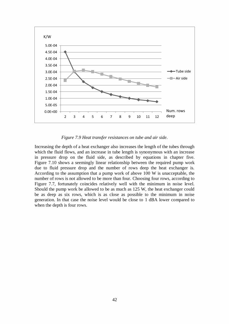
42

Figure ‎7.9 Heat transfer resistances on tube and air side.

Increasing the depth of a heat exchanger also increases the length of the tubes through

which the fluid flows, and an increase in tube length is synonymous with an increase

in pressure drop on the fluid side, as described by equations in chapter five.

Figure 7.10 shows a seemingly linear relationship between the required pump work

due to fluid pressure drop and the number of rows deep the heat exchanger is.

According to the assumption that a pump work of above 100 W is unacceptable, the

number of rows is not allowed to be more than four. Choosing four rows, according to

Figure 7.7, fortunately coincides relatively well with the minimum in noise level.

Should the pump work be allowed to be as much as 125 W, the heat exchanger could

be as deep as six rows, which is as close as possible to the minimum in noise

generation. In that case the noise level would be close to 1 dBA lower compared to

when the depth is four rows.

0.0E+00

5.0E-05

1.0E-04

1.5E-04

2.0E-04

2.5E-04

3.0E-04

3.5E-04

4.0E-04

4.5E-04

5.0E-04

2 3 4 5 6 7 8 9 10 11 12

Tube side

Air side

Num. rows deep

K/W

43

Figure ‎7.10 Required pump work as a function of numbers of rows deep.

The mass flow of brine has in each model consistently been kept at 1 kg/s. This may

however not necessarily be the case, and for that reason it is shown in Figure 7.11

what the impact on noise level is if the mass flow is changed. The figure shows that it

makes a significant difference in noise level what the mass flow is set to be. In fact, as

a result of the reduction in heat transfer resistance on the fluid side as a consequence

of a higher mass flow, the noise level can be reduced about 2 dBA if the mass flow is

increased from 1 to 1.5 kg/s. An even larger difference in noise level is seen when

comparing a case where the mass flow is 0.5 and the case where it is 1 kg/s, as can be

observed in Figure 7.11. However, increasing the fluid mass flow has a significant

impact on the required pump work, evident in Figure 7.12. To stay below 100 W of

pump work, choosing a mass flow of 1 kg/s appears to be a suitable decision.

0

50

100

150

200

250

300

2 3 4 5 6 7 8 9 10 11 12

Num. rows deep

W

44

Figure ‎7.11 Noise level as a function of fluid mass flow.

Figure ‎7.12 Required pump work as a function of fluid mass flow.

0

10

20

30

40

50

60

70

0.5 1 1.5

dBA

kg/s

0

20

40

60

80

100

120

140

160

180

200

0.5 1 1.5 kg/s

W

45

7.3 Contingency analysis

The results of this study are based on a number of assumptions, meaning that there is

good chance of a different outcome of the heat exchanger modeling if the assumptions

were to be made differently. A selection of two assumptions has been made and will

be subject to analysis in order to determine their impact on the results. One is the way

the inlet temperature of brine is determined, and the other is the way the noise level is

theoretically calculated. These two were chosen since they were suspected of having a

large impact on the results.

In the chapter where it is described how to theoretically calculate the noise level, it is

mentioned that a number of so called values given in ASHRAE (2009) are

swapped for values that have been found in unpublished laboratory measurements.

The numbers given in ASHRAE (2009) are higher than the numbers that were used to

replace them, why if using the numbers given in ASHRAE (2009), the calculated

noise levels would have a tendency to be higher. For this reason, all modeled heat

exchangers would need to be larger, since air flow and pressure drop would need to be

lower in order for the noise level not to exceed the limit of 56 dBA. The same

values were used in all cases, and for that reason it makes no difference when ranking

the four heat exchangers which values are used. However, in absolute values it

does make a difference which values that are chosen. If running the model and

instead using the values of ASHRAE (2009), the necessary volume of the FFT1 heat

exchanger is around 0.06 m3, which is actually about 40% to 50% larger than the

volume presented in the result. The values taken from the laboratory tests are seen

as better valid for the working range and for the specific application, thus using these

is assumed to give the more accurate result.

As stated in chapter 3.3, assumptions were made in order to determine the inlet

temperature of the brine that needed to be used in the model. One of the assumptions

was the minimum temperature difference between the air and refrigerant in the

reference heat exchanger that affects the brine inlet temperature. If the inlet brine

temperature would be assumed to be higher, the resulting necessary heat exchanger

volume would be larger. Similarly, if the inlet temperature would be assumed to be

lower, the resulting necessary volume would be smaller. The early assumptions about

brine temperature therefore impact the results of the heat exchanger ranking. All four

heat exchangers are however modeled under the same assumption, which mitigates

the effects of the inlet brine temperature when determining which one considered to

be the best. To give an idea of how large the difference would be in absolute numbers,

if the inlet brine temperature was set 1 ºC higher, the resulting volume was about 20

% larger for the FFT1 heat exchanger. If the inlet temperature was set 1 ºC lower, the

resulting volume was about 13 % smaller for FFT1.

47

8 Conclusions

This chapter contains a list of conclusions drawn from having made this study. The

list contains only brief statements, and more in depth motivations and explanations are

found in previous chapters.

From a noise perspective, the two heat exchangers with flat tubes are

significantly more preferable than both heat exchangers with round tubes,

since they do not need to be as large in size, and therefore are assumed to also

be less expensive. More specifically, the two flat tube heat exchangers can, at

a lower cost, be used to achieve the same heat transfer rate while still not

generating more noise than any of the round tube heat exchangers.

Out of the two heat exchangers with flat tubes, the one with plain fins is

preferable from a noise perspective. Wavy fins increase the heat transfer rate,

but at the expense of noise generation. Thus, plain fins are preferable if low

noise and small size is desired. However, the difference it makes using one

type of fin geometry or the other is relatively small and in fact possibly

negligible.

If keeping all dimensions except frontal area of the heat exchanger with flat

tubes and plain fins constant, the noise generation decreases noticeably and

steadily as a function of increase in frontal area. If the heat exchanger is 4

rows deep, the noise level is expected to decrease by about 1 dBA per every

0.017 m2 that is added to the frontal area. In order not to exceed a noise level

of 56 dBA, the frontal area needs to be at least 0.49 m2.

As for the heat exchanger with flat tubes and plain fins, in order not to exceed

the limit of 100 W of required pump work on the fluid side, the number of

circuits should not be more than one. Increasing the number of circuits has

only minor positive effects from a noise perspective, however happens at a

large expense of required pump work on the fluid side.

When analyzing the impact on noise generation as a function of using a heat

exchanger with flat tubes and plain fins that is two to twelve rows deep, there

is a minimum in noise generation at around four rows. Hence, having fewer or

more rows than four is not preferable from a noise perspective.

If the fluid flowing through the heat exchanger with flat tubes and plain fins is

kept at a mass flow of 1 kg/s, the fluid pump work is kept below 100 W. If the

mass flow is increased by 50 %, the noise level is expected to decrease

noticeably, but at a large expense of pump work. Decreasing the mass flow

with 50 % will decrease the pump work, but also significantly increase the

noise level. For that reason, a mass flow of 1 kg/s is concluded to be suitable.

Taking all conclusions above into consideration, it can be concluded that, out of the

four different heat exchangers tested, it is the one with flat tubes and plain fins that is

preferable given all the conditions. The unit should be 44 rows high (701 mm), 4 rows

deep (79 mm), have a width of 701 mm, one circuit, and be fed with a mass flow of

brine of 1 kg/s.

49

9 Recommendations for further studies

To further evaluate flat and round tube heat exchangers for indirect heat pump

systems, one parameter to elaborate is the outdoor air condition. As in the paper

Swedish Standards Institute (2011) there are other standardized temperatures to test

and evaluate. A higher number of test points, and thereby results, would be useful to

the depth of the study.

As the investigated heat exchangers are parts in a larger heat pump system,

constructed for the residential building market, an in depth price investigation would

give a more complete picture of the possibilities to implement flat tube heat

exchangers. Parameters to be investigated would for example be development and

manufacturing cost for each different design.

Furthermore to validate the results, laboratory measurements can be carried out and

compared to the computer modeled outcome.

50

References

ASHRAE (2009): 2009 ASHRAE HANDBOOK – FUNDAMENTALS Inch-Pound

Edition, Editor – Mark S. Owen, Atlanta.

Fredrik Karlsson, researcher at SP Technical Research Institute of Sweden, Personal

communication.

Gnielinski, V., (1989): Zur Wärmeübertragung bei laminarer Rohrströmung und

konstanter Wandtemperatur (In German), Chemieningenieurtechnik 61 p.160-161.

Granryd, E., (2007): International Congress of Refrigeration. Beijing. Optimum flow

rates in indirect systems. ICR07-B1-1376.

Gustafsson, O. PhD student at Chalmers University of Technology, Personal

communication.

Haglund Stignor, C., (2009): Laminar-flow Liquid-to-air Heat Exchangers – Energy-

efficient Display Cabinet Applications. Lund: Lund University.

Haglund Stignor, C., (2002): Liquid Side Heat Transfer and Pressure Drop in Finned-

Tube Cooling-Coils. Lund: Lund Institute if Technology.

Hrnjak, P. S., (1997): ASHRAE/NIST Refrigerants Conference. The Benefits and

Penalties Associated with the use of Secondary Loops. October 1997 Gaithersburg.

Incropera, F. P., DeWitt, D.P., Berman, T.L., and Lavine, A.S., (2007): Fundamentals

of Heat and Mass Transfer. 6th ed. New York: John Wiley & Sons.

IVT, (2013): IVT PremiumLine A Plus Luft/vattenvärmepump (In Swedish). [pdf].

Available at: <http://doc.ivt.se/download.asp?pt=se&fn=Pr_bl_PremiumLine-

APlus.pdf> [Accessed 13 August 2013].

Jacobi, A. M., Park Y., Zhong, Y., Michna, G., and Xia, Y., (2005): High

Performance Heat Exchangers for Air-Conditioning and Refrigeration Applications

(Non-Circular Tubes), Air- Conditioning and Refrigeration Technology Institute

(ARTI), July.

Jacobi, A. M., and Xia, Y., (2005): Air-Side Data Interpretation and Performance

Analysis for Heat Exchangers with Simultaneous Heat and Mass Transfer: Wet and

51

Frosted Surfaces, International Journal of Heat and Mass Transfer, vol. 48, no. 25-

26. pp. 5089-5102.

Kakaç, S., Liu, H. and Pramuanjaroenkij, A., (2012): Heat Exchangers Selection,

Rating, and Thermal Design. Taylor & Francis Group, Boca Raton.

Kays, W. M. and London, A.L., (1984): Compact Heat Exchangers. 3rd ed. McGraw-

Hill, New York.

MEGlobal, (2013): Ethylene Glycol Product Guide. [pdf]. Available at:

<http://www.meglobal.biz/media/product_guides/MEGlobal_MEG.pdf> [Accessed

10th of August 2013].

Nibe, (2013): Installatörshandbok NIBE F2030 Luft/vatten-värmepump (In Swedish).

[pdf]. Available at: <http://www.nibeonline.com/pdf/231107-1.pdf> [Accessed 13

August 2013].

Shah, R., K., and Sekulić, D,. P., (2003): Fundamentals of heat exchanger design.

John Wiley & Sons. Hoboken, New Jersey.

Shah, R.K. and London, A. L., (1978): Laminar flow forced convection in ducts: a

source book for compact heat exchanger analytical data. Academic press, New York.

Smith, B., J., (2011): Acoustics and noise control. Prentice Hall, Harlow.

Svenska Kyltekniska Föreningen (2010): Handbook on indirect refrigeration and heat

pump system, Melinder, Å., Kullavik, Sweden.

Swedish Standards Institute (2011): Air conditioners, liquid chilling packages and

heat pumps with electrical driven compressors for space heating and cooling – Part

2. : Test conditions. SS-EN 14511-2:2011, Stockholm.

Swedish Energy Agency (a), Luftvattenvärmepumpar (In Swedish) ( Air to water heat

pumps)Availableat:<https://www.energimyndigheten.se/Hushall/Testerresultat/Testre

sultat/Luftvattenvarmepumpar1/?tab=2> [Accessed 1th of July 2013].

Swedish Energy Agency (b), Circulationspumpar (In Swedish) (Circulation pumps)

Available at: http://www.energimyndigheten.se/Hushall/Testerresultat/Testresultat/

Cirkulationspumpar/?tab=2 [Accessed 1th

of July 2013].

52

Thermia, (2013): Thermia Atria Optimum Atria Duo Optimum (In Swedish). [pdf].

Available at: <http://www.thermia.se/docroot/dokumentbank/Thermia-Varmepumpar-

AtriaOptimum-AtriaDuoOptimum.pdf> [Accessed 12 June 2013].

Thermia, (2010): Installationsanvisning (In Swedish). [pdf]. Private e-mail from

Thermia-Danfoss Värmepumpar Aktiebolag.

White, F. M., (2011): Fluid Meachanics.7th ed. McGraw-Hill, New York.

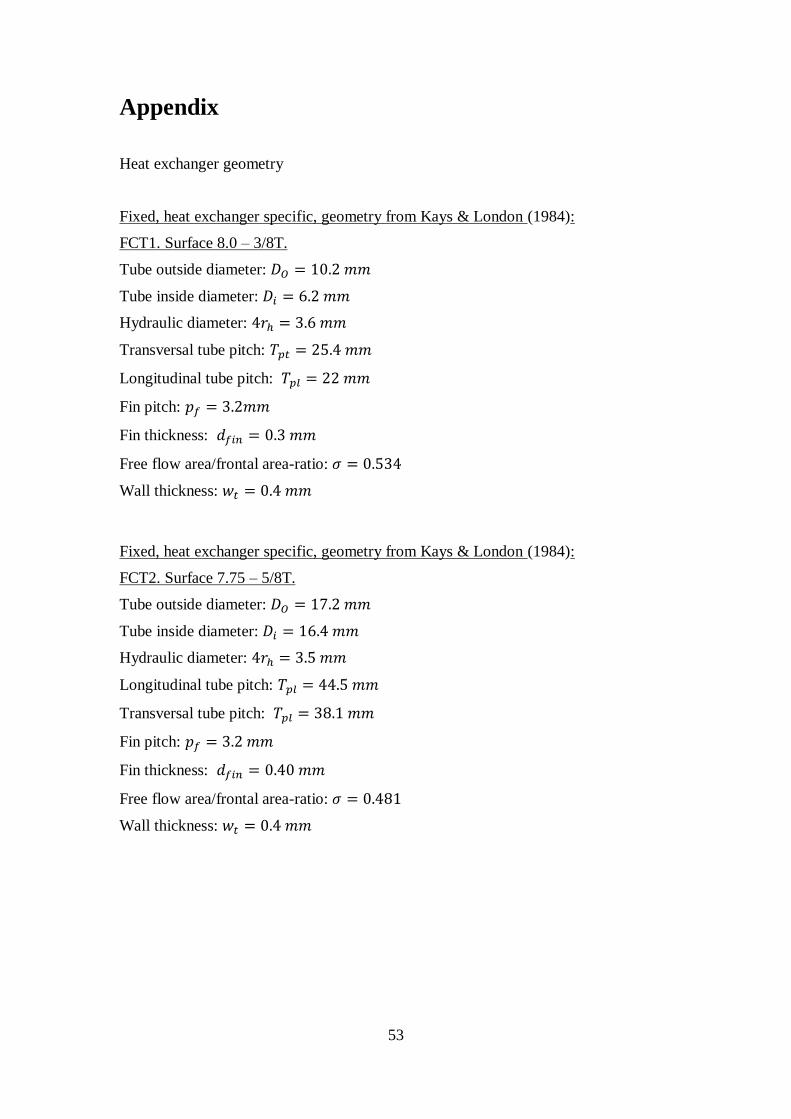
53

Appendix

Heat exchanger geometry

Fixed, heat exchanger specific, geometry from Kays & London (1984):

FCT1. Surface 8.0 – 3/8T.

Tube outside diameter:

Tube inside diameter:

Hydraulic diameter:

Transversal tube pitch:

Longitudinal tube pitch:

Fin pitch:

Fin thickness:

Free flow area/frontal area-ratio:

Wall thickness:


FCT2. Surface 7.75 – 5/8T.

Tube outside diameter:

Tube inside diameter:

Hydraulic diameter:

Longitudinal tube pitch:


Fin pitch:

Fin thickness:


Wall thickness:

54


FFT1. Surface 9.1 – 0.737-S

Tube height:

Tube length:

Hydraulic diameter:


Longitudinal tube spacing:

Fin pitch:

Fin thickness:


Wall thickness:


FFT2. Surface 9.29 – 0.737-SR

Tube height:

Tube length:

Hydraulic diameter:


Longitudinal tube spacing:

Fin pitch:

Fin thickness:


Wall thickness:

Design aspects related to noise in indirect heat...

Documents

Transcript of Design aspects related to noise in indirect heat...