Project Number: MAD-005A

Design and Testing of a

Large Flexible Space Structure

A Major Qualifying Project Report

submitted to the Faculty

of the

WORCESTER POLYTECHNIC INSTITUTE

in partial fulfillment of the requirements for the

Degree of Bachelor of Science

By

_______________ ________________ _______________

Thomas Angell Rebecca O'Neil Kevin Rugani

Date: March 3, 2006

Approved:

_______________________________________

Professor Michael A. Demetriou, Major Advisor

Abstract

This project's objective was to design and build a flat plate structure for testing the

effectiveness of piezoceramic (PZT) patches as actuating and sensing devices for the

vibration suppression of actively controlled structures. The plate was excited to its natural

frequencies and controlled by a decentralized output feedback strategy with three collocated

actuator/sensor pairs. The vibration levels were significantly reduced thereby validating the

use of PZT as integrated actuator/sensors pairs in vibration suppression of actively controlled

structures.

- i -

Acknowledgements

• Raffaele Potami, for guidance in design and testing of the structure throughout the

duration of the project.

• Professor Michael A. Demetriou, for guidance in the design and testing of the

controls for the project.

• Higgins Machine Shop, for assisting in the construction of the structure.

- ii -

Table of Contents

Abstract ................................................................................................................................. i Acknowledgements .............................................................................................................. ii Table of Contents................................................................................................................ iii List of Figures ..................................................................................................................... iv List of Tables ....................................................................................................................... iv 1 Introduction....................................................................................................................... 1 2 Space Structures and Vibration ...................................................................................... 2

2.1 Flexible Space Structures ............................................................................................ 2 2.2 Vibration of Structures in Space.................................................................................. 3 2.3 Vibration Suppression ................................................................................................. 3 2.4 Piezoelectric Sensors................................................................................................... 4 2.5 Two Dimensional Plates.............................................................................................. 5 2.6 Natural Frequency and Mode Shape........................................................................... 6 2.7 Vibration Isolation Table............................................................................................. 7

3 Frequency Calculations and Plate Sizing ....................................................................... 8 3.1 Design Considerations .............................................................................................. 10 3.2 Final Design .............................................................................................................. 11 3.3 Piezoelectric Patch Attachment................................................................................. 11

4 Experiment Set-Up ......................................................................................................... 14 4.1 Signal Generation...................................................................................................... 15 4.2 Signal Sensing ........................................................................................................... 16 4.3 Vibration Control ...................................................................................................... 19

5 Natural Frequency Verification .................................................................................... 20 5.1 Vibration Reduction Testing...................................................................................... 22 5.2 Vibration Reduction Analysis .................................................................................... 23

6 Future Testing and Application .................................................................................... 24 Appendix A: Clamp Design Drawings ................................................................................ 25 Appendix B: Table of Equipment........................................................................................ 33 Appendix C: MatLab FFT Analysis Code........................................................................... 34 References............................................................................................................................ 35

- iii -

List of Figures

Figure 2.1: Modal shape 2.1 ......................................................................................................6 Figure 3.1: Natural frequency vs. side length............................................................................9 Figure 3.2: Natural frequency vs. thickness (side length = 1m). ...............................................9 Figure 3.3: Optimal piezoelectric patch placement. ................................................................13 Figure 3.4: Experimental patch placement. .............................................................................13 Figure 4.1: Experimental set up...............................................................................................14 Figure 4.2: Instek® function generator.....................................................................................15 Figure 4.3: AVC® 790 series power amplifier.........................................................................15 Figure 4.4: Comdyna GP-6 operational amplifier. ..................................................................16 Figure 4.5: Krohn-Hite® signal filter. ......................................................................................17 Figure 4.6: dSpace® control board...........................................................................................17 Figure 4.7: Simulink® display, configured vibration cancellation...........................................18 Figure 4.8: ControlDesk® program display for vibration cancellation. ...................................19 Figure 5.1: Accelerometer and sensor vibration readings. ......................................................20 Figure 5.2: Accelerometer and sensor FFT comparison..........................................................21

List of Tables

Table 2.1: Modal shape values. .................................................................................................7 Table 3.2: Plate properties. ......................................................................................................10 Table 5.1: Root mean square values for sensor voltage. .........................................................23 Table 5.2 Percent reduction of sensor voltage.........................................................................23

- iv -

1 Introduction

As research in space has become more complex, similarly has the design of new

space structures. Researchers are now looking to platforms which can gather a variety of

information, are self sustaining, and test the limits of what we know is capable in space. The

uses and abilities of flexible space structures are constantly changing and expanding, in

addition to the need to know that such structures will be able to withstand whatever forces

they may encounter in space. Therefore, it is important to investigate possible causes and

effects of vibrations on flexible space structures, as well as evaluate what methods might be

best for suppressing such vibrations.

Currently, research is being done on forms of "active damping" to control vibration of

structures in space. This entails the use of piezoelectric patches that convert mechanical

energy to electrical energy and vice versa. By these means, it is possible to determine the

nature of the vibration on a particular structure and effectively counter and reduce that

vibration. One of the most important aspects of this technology is determining the placement

of the patches on a particular structure.

At Worcester Polytechnic Institute, there has been ongoing research on this topic

using one-dimensional beam structures. However, one-dimensional construction is not

common in the more complex space structures present today. Therefore, it is important to

expand the research to two-dimensional flat plates, similar to solar panels present on virtually

every space structure in use. The purpose of this project is to design a build a flat plate

structure and numerically and experimentally determine how the location of the piezoelectric

patches affects the active damping within the two-dimensional plate.

- 1 -

2 Space Structures and Vibration

2.1 Flexible Space Structures

In the past, the construction of space structures was focused on large truss bodies. For

example, satellites or large mirrors that were built on Earth with the intention of being as

stable and resilient as possible. One problem with this approach was that sometimes while

attempting to make a structure more resistant to failure or breakage, the structure became too

cumbersome or costly. More recent space technology points to lighter and cheaper designs in

light of these past problems and the emergent desire of public and private sources to

contribute to the space-research industry. NASA isolates a few specific requirements of

material properties which apply to the design of space structures, many of them, not

surprisingly, relate to cost effectiveness [1]. For example, weight: to send one pound of

material into space, ten pounds of equipment must be utilized here on Earth. The material

must be dimensionally stable, meaning it cannot shrink or expand due to extreme

temperatures in space. It must also be able to endure the harsh environment of space which

consists of a vacuum often containing radiation, debris and other elements not found on Earth.

Sometimes, a material that meets all these other requirements is that which humans cannot

physically withstand. In the case that humans can not handle, test or assemble the product, it

would also be ruled out of eligibility. It is beginning to seem impossible to meet all the

requirements at once, so is all this stress about the design of flexible space structures really

necessary?

Well, according to NASA’s Middeck Active Control Experiment (MACE), the need

for more flexible and durable structures in space is on the rise [2]. Today’s space structures

are becoming more and more complex. Now, researchers are designing structures with solar

- 2 -

panel attachments, moving robotic arms, sensors that scan in different directions, and other

attachments that can possibly create small vibrations within the structure.

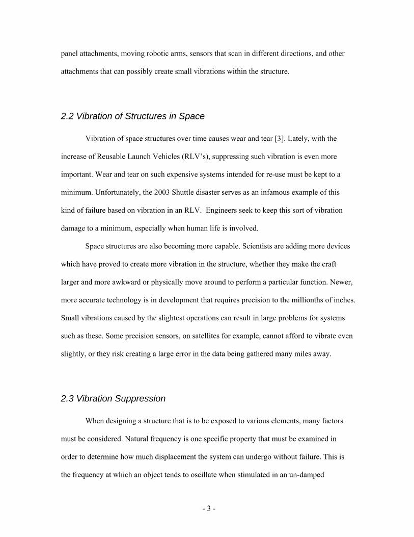
2.2 Vibration of Structures in Space

Vibration of space structures over time causes wear and tear [3]. Lately, with the

increase of Reusable Launch Vehicles (RLV’s), suppressing such vibration is even more

important. Wear and tear on such expensive systems intended for re-use must be kept to a

minimum. Unfortunately, the 2003 Shuttle disaster serves as an infamous example of this

kind of failure based on vibration in an RLV. Engineers seek to keep this sort of vibration

damage to a minimum, especially when human life is involved.

Space structures are also becoming more capable. Scientists are adding more devices

which have proved to create more vibration in the structure, whether they make the craft

larger and more awkward or physically move around to perform a particular function. Newer,

more accurate technology is in development that requires precision to the millionths of inches.

Small vibrations caused by the slightest operations can result in large problems for systems

such as these. Some precision sensors, on satellites for example, cannot afford to vibrate even

slightly, or they risk creating a large error in the data being gathered many miles away.

2.3 Vibration Suppression

When designing a structure that is to be exposed to various elements, many factors

must be considered. Natural frequency is one specific property that must be examined in

order to determine how much displacement the system can undergo without failure. This is

the frequency at which an object tends to oscillate when stimulated in an un-damped

- 3 -

environment. If the natural frequency is exceeded the system could fail. This is why the

process of suppressing vibrations in an object, or damping the system, is so important [4].

The two basic types of damping are Active and Passive. Passive Vibration

Suppression involves damping of vibrations through features included within the structure or

internal structural specifications, which resist and suppress vibration. Active Vibration

Suppression involves damping of vibrations through means not included within the system

itself, in other words, applying an outside force to counterbalance some vibration within the

structure.

Stiffness is one example of passive suppression. This and other characteristics of

materials are very important for determining how a structure will react to vibration. Qualities

of the material used can be evaluated to show how the object will resonate and play a large

role in determining what material is best for certain space structures. Another important

factor in passive vibration is how parts are fitted together or joined. Different types of joints

are better or worse at damping vibrations that may travel between two parts.

Actuators are one commonly used type of active suppression. This is a type of

transducer that allows some agent to work through it. There are many kinds of actuators, but

for engineering purposes, the important kind is one that sends an electrical signal which is

transformed into equal and opposite force with relation to an apparent vibration in the space

structure.

2.4 Piezoelectric Sensors

The piezoelectric effect involves a material that produces an electric charge when any

force is applied to it [5]. Scientists have also discovered how to use this effect conversely in

what is known as the inverse piezoelectric effect, which states that an electric charge can be

- 4 -

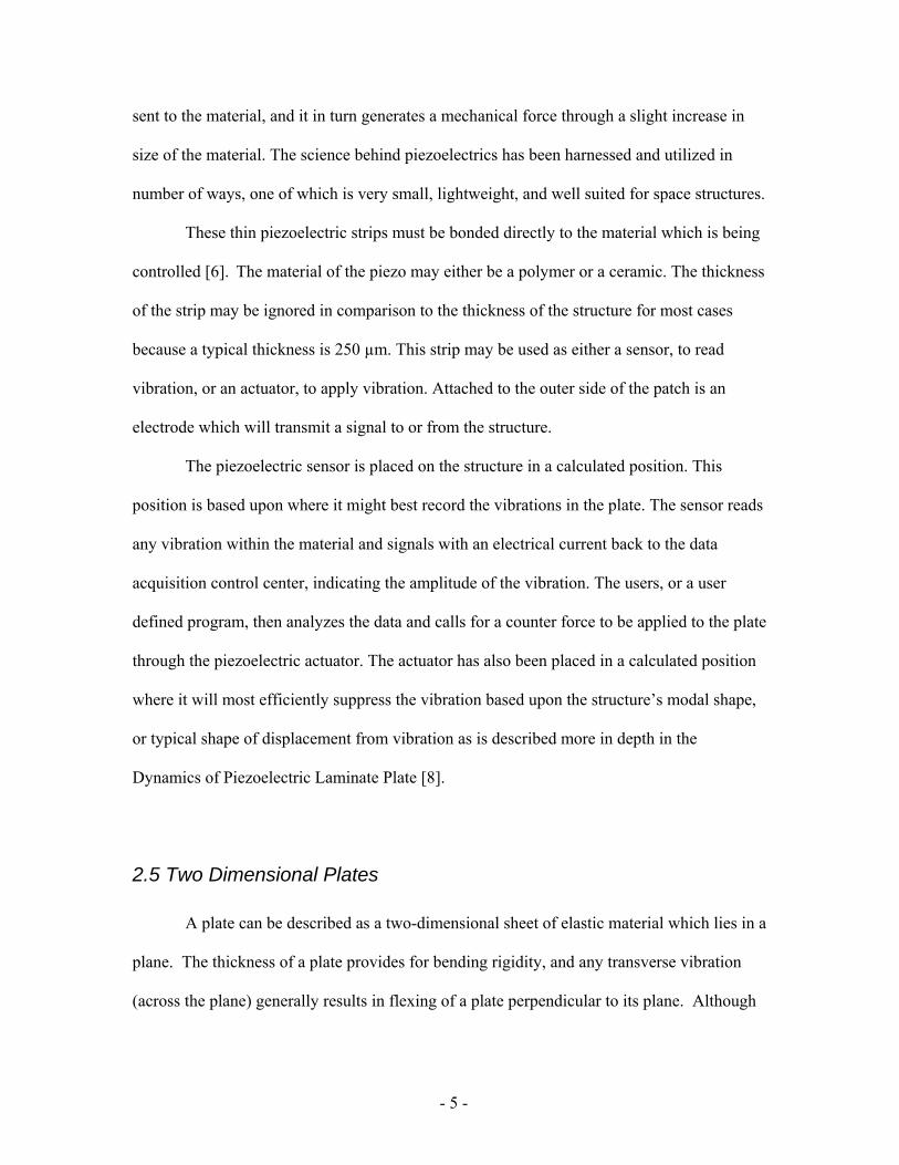
sent to the material, and it in turn generates a mechanical force through a slight increase in

size of the material. The science behind piezoelectrics has been harnessed and utilized in

number of ways, one of which is very small, lightweight, and well suited for space structures.

These thin piezoelectric strips must be bonded directly to the material which is being

controlled [6]. The material of the piezo may either be a polymer or a ceramic. The thickness

of the strip may be ignored in comparison to the thickness of the structure for most cases

because a typical thickness is 250 µm. This strip may be used as either a sensor, to read

vibration, or an actuator, to apply vibration. Attached to the outer side of the patch is an

electrode which will transmit a signal to or from the structure.

The piezoelectric sensor is placed on the structure in a calculated position. This

position is based upon where it might best record the vibrations in the plate. The sensor reads

any vibration within the material and signals with an electrical current back to the data

acquisition control center, indicating the amplitude of the vibration. The users, or a user

defined program, then analyzes the data and calls for a counter force to be applied to the plate

through the piezoelectric actuator. The actuator has also been placed in a calculated position

where it will most efficiently suppress the vibration based upon the structure’s modal shape,

or typical shape of displacement from vibration as is described more in depth in the

Dynamics of Piezoelectric Laminate Plate [8].

2.5 Two Dimensional Plates

A plate can be described as a two-dimensional sheet of elastic material which lies in a

plane. The thickness of a plate provides for bending rigidity, and any transverse vibration

(across the plane) generally results in flexing of a plate perpendicular to its plane. Although

- 5 -

every plate has some thickness, it can be assumed two-dimensional (for calculation purposes)

if the plate thickness is less than 1/10 the shortest planar length [9].

2.6 Natural Frequency and Mode Shape

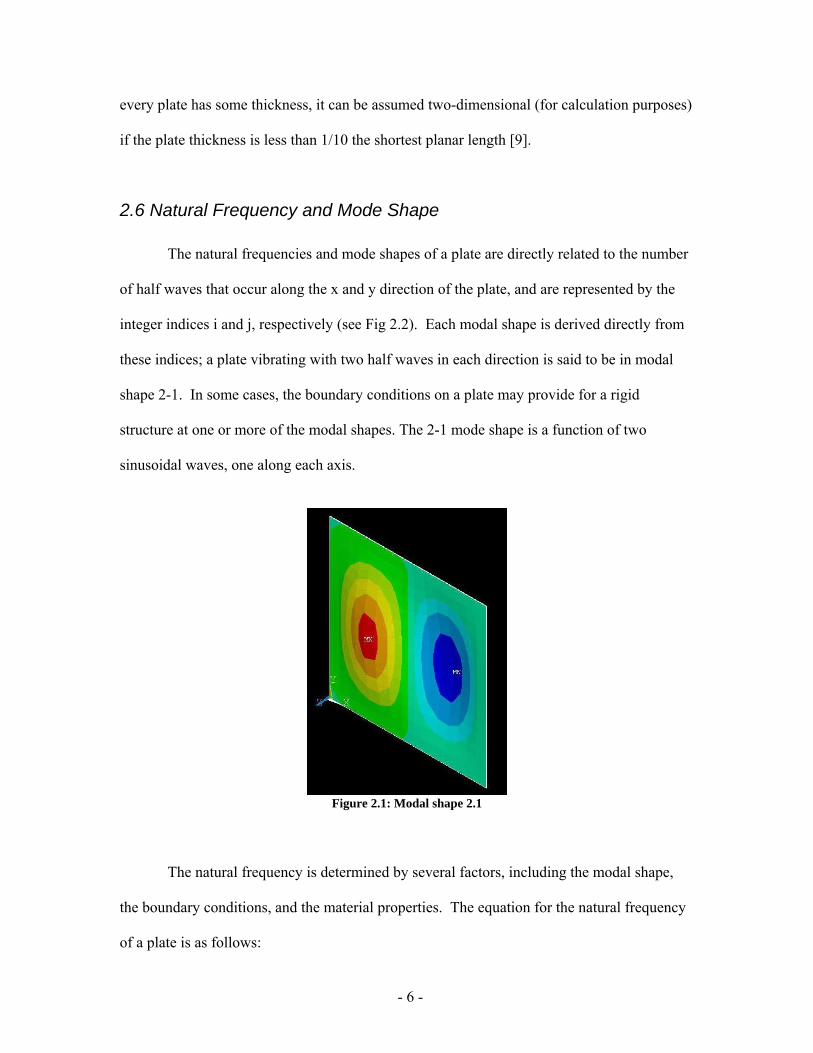
The natural frequencies and mode shapes of a plate are directly related to the number

of half waves that occur along the x and y direction of the plate, and are represented by the

integer indices i and j, respectively (see Fig 2.2). Each modal shape is derived directly from

these indices; a plate vibrating with two half waves in each direction is said to be in modal

shape 2-1. In some cases, the boundary conditions on a plate may provide for a rigid

structure at one or more of the modal shapes. The 2-1 mode shape is a function of two

sinusoidal waves, one along each axis.

Figure 2.1: Modal shape 2.1

The natural frequency is determined by several factors, including the modal shape,

the boundary conditions, and the material properties. The equation for the natural frequency

of a plate is as follows:

- 6 -

( )2/1

2

3

2

2

1122 ⎥⎦

⎤⎢⎣

⎡−

=υγπ

λ Eha

f ij

ij i=1, 2, 3… j=1, 2, 3…

Equation 1: Natural frequency.

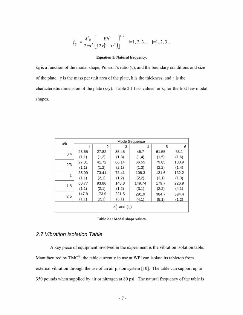
λij is a function of the modal shape, Poisson’s ratio (ν), and the boundary conditions and size

of the plate. γ is the mass per unit area of the plate, h is the thickness, and a is the

characteristic dimension of the plate (x/y). Table 2.1 lists values for λij for the first few modal

shapes.

Mode Sequence a/b 1 2 3 4 5 6

23.65 27.82 35.45 46.7 61.55 63.1 0.4

(1,1) (1,2) (1,3) (1,4) (1,5) (1,6) 27.01 41.72 66.14 66.55 79.85 100.9

2/3 (1,1) (1,2) (2,1) (1,3) (2,2) (1,4) 35.99 73.41 73.41 108.3 131.6 132.2

1 (1,1) (2,1) (1,2) (2,2) (3,1) (1,3) 60.77 93.86 148.8 149.74 179.7 226.9

1.5 (1,1) (2,1) (1,2) (3,1) (2,2) (4,1) 147.8 173.9 221.5 291.9 384.7 394.4 2.5 (1,1) (2,1) (3,1) (4,1) (5,1) (1,2)

and (i,j) 2ijλ

Table 2.1: Modal shape values.

2.7 Vibration Isolation Table

A key piece of equipment involved in the experiment is the vibration isolation table.

Manufactured by TMC®, the table currently in use at WPI can isolate its tabletop from

external vibration through the use of an air piston system [10]. The table can support up to

350 pounds when supplied by air or nitrogen at 80 psi. The natural frequency of the table is

- 7 -

around 1.0 Hz in both the horizontal and vertical directions, which is much lower than the

natural frequency of the plate and the sensitivity of the data acquisition system. The table

will ensure that no external forces affect the data measurement of the actual plate structure.

3 Frequency Calculations and Plate Sizing

One of the limiting factors in designing the plate structure was the sensitivity of the

data acquisition system. The operating range of the system is between 15 Hz to 1000 Hz. In

the interest of safety, it was decided to go no higher than 50% of the system’s capability.

This limitation resulted in an experimental frequency of no higher than 500 Hz, which was

only capable of stimulating the first few natural frequencies.

Equation (1) provided the basis for the initial frequency calculations of the plate,

using values of λij provided by Blevins [11] (See Table 3.1). The main goal was to

determine what plate properties would give a first natural frequency (modal shape 1-1) close

to the low end constraint of 15 Hz. The plate material was chosen to be aluminum, which

meant the only other two properties of the plate that could change the natural frequency were

the side length and the thickness. Figures 3 and 4 show how each parameter affected the

natural frequency of the plate.

With the side length as the variable, the line was hardly linear. Large plate sizes had

small variances in natural frequency, while small plate sizes had large variances in natural

frequency. In order to obtain a first natural frequency of approximately 15 Hz, the plate

would to have been about 1.4 meters on a side – somewhat large for the vibration suppression

lab table to hold. With the plate thickness as the variable, the line became much more linear,

allowing the first natural frequency to remain relatively low over a range of thicknesses. The

- 8 -

best feature of a variable thickness and fixed side length was that it was much simpler to

make use of a standard frame and vary the plate thickness to obtain different frequencies.

y = 18.053x-2

0.00

50.00

100.00

150.00

200.00

250.00

300.00

350.00

400.00

450.00

500.00

0 0.5 1 1.5 2 2.5

Side Length (m)

Nat

ural

Fre

quen

cy (H

z)

Series1Power (Series1)

Figure 3.1: Natural frequency vs. side length.

y = 282080x1.5

0.00

20.00

40.00

60.00

80.00

100.00

120.00

140.00

0 0.001 0.002 0.003 0.004 0.005 0.006 0.007

Thickness (m)

Nat

ural

Fre

quen

cy (H

z)

Series1Power (Series1)

Figure 3.2: Natural frequency vs. thickness (side length = 1m).

- 9 -

After deciding to use the plate thickness as the variable, it was possible to find out

what thickness would correspond to a 15 Hz frequency on a one meter square plate. Using

equation 1, it was determined that a frequency of slightly under 15 Hz resulted from a stock

plate thickness of 1.4 millimeters. In order to ensure that the data acquisition system was

operating within its limits, it was decided to go with a 1.6 millimeter thick plate with a first

natural frequency of just over 18 Hz. Tables 2.1 and 3.1 show the frequency values and plate

properties used in the calculations.

Plate Properties

Elastic Modulus:10109.6 × 2m

N

Poisson's Ratio: 0.35

Thickness: 0.0016 m

Side Length: 1 m

Mass: 4.341 kg

Area: 12m

Table 3.1: Plate properties.

3.1 Design Considerations

In order to perform vibration testing, a suitable design to firmly clamp and support

our aluminum plate was needed. Making use of a vertically clamped plate seemed best, as a

horizontally aligned plate would be prone to more severe bending under its own weight,

possibly affecting the natural frequency. Second, due to constraints of the experiment, the

aluminum plate had to be fully clamped on all four edges to simulate a typical aerospace

- 10 -

plate design. Screws, C-clamps, and a specially carved groove were the options considered

for clamping, and each are encompassed in individual designs. As previously stated, the

decision was made to use a one meter square plate for ease in mathematical calculations.

Steel was chosen as a building material for reasons of cost, stiffness, availability, and

material frequency. Since vibrations were passing through the aluminum plate, the

framework structure had to be made of something other than aluminum or else the structure

would have been prone to vibration as well. ProEngineer® was the modeling software of

choice to use for our designs, as parts were able to be created individually and assembled

fairly easily.

3.2 Final Design

After consideration of the several design concepts, it was decided that the clamp

design would be the best from both a machining and testing point of view. With the clamp

design, a very minimal amount of machining was needed and the amount of screws used in

this design was far less than that of the bolt design. The weight of the structure was

calculated to be about 220 pounds, well under the 350 pound weight limit of the lab table

used for the experiment. Based on these factors, it was decided that the clamp design was the

best option for the experiment. Appendix A provides detailed drawings of the flat plate

structure and configurations.

3.3 Piezoelectric Patch Attachment

There are a variety of aspects to consider when attaching the piezoelectric patches. A

plan for the number of patches, their placement, and a method for attaching them needs to be

- 11 -

established and then followed closely. A patch in the wrong place or not attached as closely

as necessary would cause critical errors in the experimental data.

Eight patches were attached to the aluminum sheet. Three of these were configured to

act as passive vibration sensors and the other five were configured to act as active controls to

either create or stop plate vibration. This total number of patches was selected because it was

thought to be the fewest number that would have the most influence on the plate.

Using extensive calculations, Raffaele Potami - a PhD student at WPI, was able to

determine the optimal placement of the patches. These calculations take into consideration

the size and shape of the plate, the boundary conditions and the frequency of the vibrations

amongst other things. The general idea of patch placement is to find points which have some

amplitude over a variety of frequencies and modal shapes, thus allowing the patches to be

useful over a variety of conditions. If a patch is placed at a point where a node occurs at

some frequency, it will not collect any data, and similarly will not be able to send any data.

In a paper by Demetriou and Potami, the location of optimal patch placement is explained as

"…the perfect balance between the energy that can be transferred to the structure and the

controllability over the different modal shapes" [12]. The placement of the patches on either

side of the plate is symmetrical, which is critical to the data collection and stimulation on the

plate. Optimization depends mostly on placement where it is most efficient to apply an

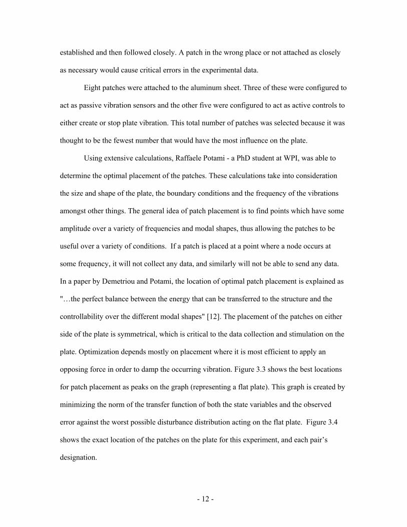
opposing force in order to damp the occurring vibration. Figure 3.3 shows the best locations

for patch placement as peaks on the graph (representing a flat plate). This graph is created by

minimizing the norm of the transfer function of both the state variables and the observed

error against the worst possible disturbance distribution acting on the flat plate. Figure 3.4

shows the exact location of the patches on the plate for this experiment, and each pair’s

designation.

- 12 -

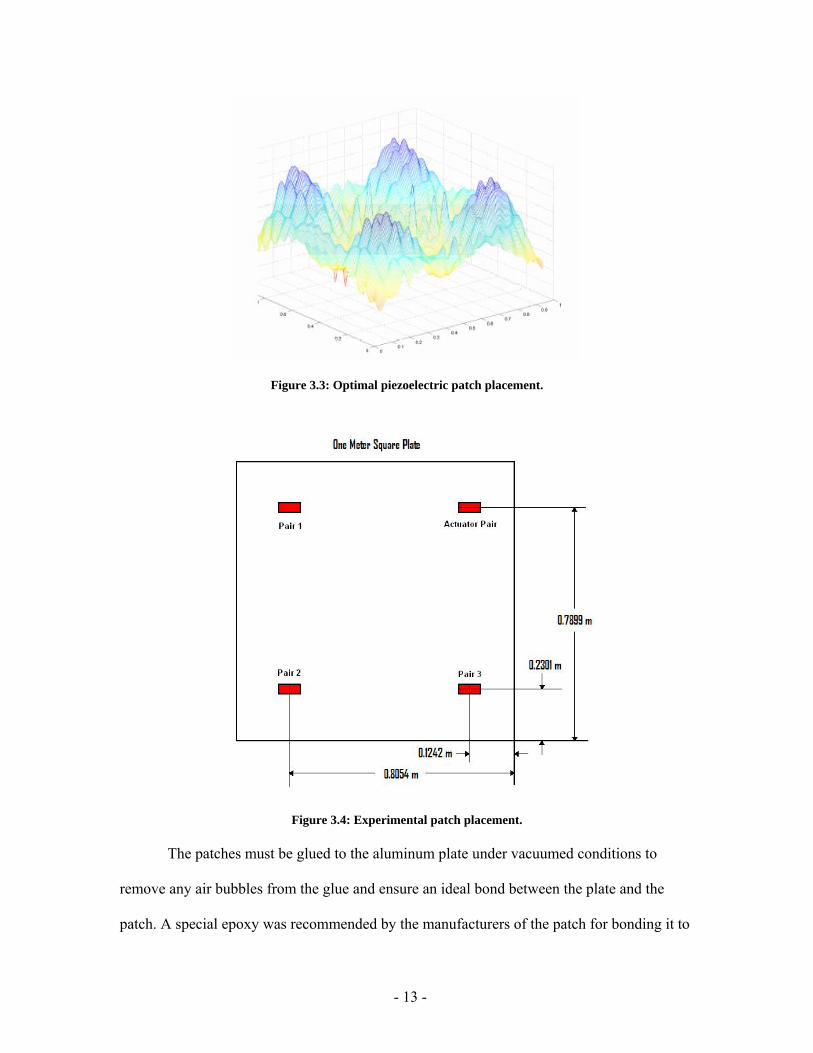
Figure 3.3: Optimal piezoelectric patch placement.

Figure 3.4: Experimental patch placement.

The patches must be glued to the aluminum plate under vacuumed conditions to

remove any air bubbles from the glue and ensure an ideal bond between the plate and the

patch. A special epoxy was recommended by the manufacturers of the patch for bonding it to

- 13 -

the aluminum surface. Once the epoxy was applied the vacuum pump had stay in place for

twenty-four hours in order to assure the integrity of the bond as the epoxy dried. This process

took ten days to glue the eight patches onto the plate. Once the patches were placed they

could not be removed or reused.

4 Experiment Set-Up

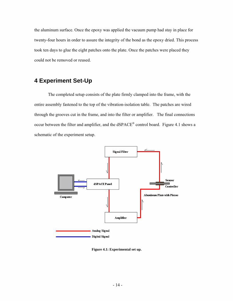
The completed setup consists of the plate firmly clamped into the frame, with the

entire assembly fastened to the top of the vibration-isolation table. The patches are wired

through the grooves cut in the frame, and into the filter or amplifier. The final connections

occur between the filter and amplifier, and the dSPACE® control board. Figure 4.1 shows a

schematic of the experiment setup.

Figure 4.1: Experimental set up.

- 14 -

4.1 Signal Generation

The initial vibration in the plate is created using several pieces of equipment. The

source of the vibration comes from an Instek® function generator (Figure 4.2) capable of

producing 0.3 Hz to 3 MHz waveform signals, and is controlled by the user throughout the

experiment.

Figure 4.2: Instek® function generator. The signal is split in two at the output of the function generator in order to activate one pair

of patches. One signal is sent directly to the AVC® 790 Series Power Amplifier (Figure 4.3),

and on to one patch.

Figure 4.3: AVC® 790 series power amplifier.

- 15 -

The other signal is sent to a Comdyna® GP-6 Operational Amplifier (Figure 4.4), where it is

negated, sent to the 790 Series Power Amplifier, and on to the second patch.

Figure 4.4: Comdyna GP-6 operational amplifier. It is necessary to negate the signal of one patch because the patches are located on either side

of the plate. While one patch is stretching, the other is squeezing, so the signals must be

opposite in gain to ensure that they are out of phase.

4.2 Signal Sensing

The signal sensing and control is accomplished through the use of a hardware and

software interface. The signal is read independently by three of the remaining six patches

(one from each pair). Each signal is filtered using a Krohn-Hite® Model 3364 Butterworth

filter (Figure 4.5), using a low pass setting at 500 Hz.

- 16 -

Figure 4.5: Krohn-Hite® signal filter. This particular value is used for several reasons: First, the hardware can only process

information at 1000 Hz or less, and 500 Hz leaves a safety margin of fifty percent. Second,

the amplitude of frequencies in the plate above 500 Hz are small enough to be naturally

damped and do not effect the testing.

From the filter, the signal is sent to the dSPACE® 1103 Control Board (Figure 4.6),

which is the interface between the hardware and software components of the setup. The

signal is converted from analog to digital or digital to analog at this point, allowing the

computer to input and output data to and from the patches. The filter is also grounded to the

digital to analog output on the board to prevent any bias from being introduced to the signal.

Figure 4.6: dSpace® control board. The three programs used to control the experiment are Matlab®, Simulink®, and

ControlDesk®. Simulink® is used to build the control software through a series of pre-made

- 17 -

or user defined "blocks". Matlab® is used to compile the programs created in Simulink®, and

ControlDesk® is designed as the user interface. Figures 4.7 and 4.8 show the Simulink® and

ControlDesk® layouts used in the experiment. Each sensor is read by the program and the

signal is displayed in ControlDesk® as the top (red) plot in each pair. The signal sent to each

controller is displayed in the bottom (blue) plots.

Figure 4.7: Simulink® display, configured vibration cancellation.

- 18 -

Figure 4.8: ControlDesk® program display for vibration cancellation.

4.3 Vibration Control

The control of the plate is based on a software implemented negative gain, and a user

controlled amplitude of each of the controllers. Since each sensor/controller pair is

independent of the others, each controller has its own gain from 0 to 1. By adjusting these

gains manually, the user is able to visually identify a reduction or amplification in the signal

being read by the sensors and adjust accordingly.

The output signal for each controller is sent to the dSPACE® 1103 Control Board and

converted from digital to analog. The voltages at this point are a maximum of 10 volts, the

output limit of the control board. Since the patches require higher voltages to be effective,

the output signals are sent to the AVC® 790 Series Power Amplifier and a gain of 20 is

applied before being sent to the patches. This ensures that the controllers can receive the

maximum 200 volts they can handle.

- 19 -

5 Natural Frequency Verification

The first tests on the plate were used to confirm the natural frequencies of the plate

that had been calculated analytically at the start of the project, and to verify that the patches

were operating correctly. An accelerometer was attached to the plate to provide the means of

verifying the plate and patch performance. The plate was set in vibration by a tap, and data

from the accelerometer and the three sensors were recorded over a period of twenty seconds

at a sample rate of 1000 Hz. Figure 5.1 shows the wave functions of the accelerometer and

three sensors.

Figure 5.1: Accelerometer and sensor vibration readings.

The data were saved as separate files for each sensor, and analyzed individually in MatLab®

using a Fast Fourier Transform (FFT). The purpose of the FFT was to determine the

- 20 -

naturally occurring frequencies of the plate by graphing each frequency over the number of

times it appeared in the dataset. A log/log axes representation of the FFT shows the natural

frequencies as peaks and valleys along the graph (Figure 5.2). The various peaks and valleys

of each sensor and the accelerometer were compared and found to be very close through the

entire range of 0-500 Hz. This confirmed that the sensors were working properly. The peaks

that occurred at 15 Hz confirmed that the first mode of the plate was close to the initial

calculation of 18 Hz. The difference in frequency of the analytical to experimental values is

due to the addition of the patches on the plate. This is confirmed by the analytical frequency

calculation of the plate. The denominator in Equation 1.1 contains the variable γ, or mass per

unit area of the plate. The added weight of the patches drives this value higher, resulting in a

larger denominator and lower frequency.

Figure 5.2: Accelerometer and sensor FFT comparison.

- 21 -

The FFT analysis of the sensors also reveals the natural frequencies of the plate,

allowing the actuators to be set to vibrate the plate at particular frequencies in order to excite

a certain mode and achieve the best displacement for vibration reduction testing. The

Matlab® code used in the FFT analysis can be found in Appendix C.

5.1 Vibration Reduction Testing

The vibration reduction testing relied on data taken at various frequencies ranging

from 15.9 Hz to 106.9 Hz. The process for recording data at each sample frequency was

made up of several steps. The first step was to activate the plate to one of its natural

frequencies using the pair of patches controlled by the function generator. By reading the

amplitude of the signal displayed by the sensors, it was easy to recognize relatively large

jumps in the amplitude of the signal as the frequency of the function generator matched a

natural frequency of the plate.

The next step was to record a dataset of the uncontrolled signal. The amplitude of the

signal in volts was taken every millisecond for a period of twenty seconds. Once that dataset

was saved, the controllers were activated by increasing the independent gains in the program.

Once a set of gains was found that created the largest reduction in amplitude of the signals

read by the sensors, another dataset of the same length was taken of the controlled signal and

saved. This process was used on four frequencies: 15.9 Hz, 44.6 Hz, 88 Hz, and 106.9 Hz.

In order to determine the magnitude of reduction in vibration on the plate, the data

from each test had to be quantified. A root mean square of the data taken by each sensor

would provide the best means of doing so. By using the following equation,

- 22 -

∑=

⋅=n

iirms V

nV

1

21 where 20001=n

Equation 5.1: Root mean square.

an average voltage of each signal over the sample length was determined. By using the

average voltage of each controlled and uncontrolled signal, the percent reduction in vibration

by each individual controller and over the entire plate was calculated (Table 5.1 and 5.2).

Table 5.1: Root mean square values for sensor voltage.

Table 5.2 Percent reduction of sensor voltage.

5.2 Vibration Reduction Analysis

The results in Tables 5.1 and 5.2 clearly show that the controllers perform better at

certain frequencies. This is due to the location of the patches in respect to the mode at which

the plate is vibrating. The peaks at each mode occur in different locations; therefore the

amplitudes experienced by the patches differ as well. When a patch experiences larger

amplitude due to vibration, its ability to control that vibration is greater. This is comparable

to a moment arm: A force applied a distance x from the origin creates a certain moment about

- 23 -

the origin. That same force applied a distance of 2·x from the origin will create a moment

twice as strong. In this case, the force is created by the patch, and the distance from the

origin is the amplitude of the signal.

Table 5.1 also shows that sensor/controller pair #2 is the most responsive in each test.

This is due to the fact that the magnitude of the amplitude of the plate is symmetrical about

the diagonal axes, regardless of the mode. Since pair #2 is diagonally opposite from the

actuating pair’s disturbance, it experiences the same amplitude.

6 Future Testing and Application

Based on the results of this experiment, active vibration control using piezoelectric

patches does work effectively in certain conditions. However, a concern of this project's

application in space is the amount of power available to control the structure. In the case of

this experiment, the power supply was unlimited, but that may not be the case in a real-world

application. One solution for this is to determine where the patches work most efficiently, in

order to consume the least amount of power.

To address this issue, it is recommended that further research be done into the

location of the patches on the plate. It is apparent from this experiment that the patches are

most effective when they are located at the peaks of each mode. Therefore, locating patch

pairs at one peak of each of the first several modes should provide more control of the

structure. Since the added mass of the patches changes the location of the peaks of each

modal shape of the plate, it is recommended that several iterations be done to determine the

best location for the patches.

- 24 -

- 25 -

Appendix A: Clamp Design Drawings

Square Aluminum Plate

- 26 -

Steel Back Frame

- 27 -

Square Steel Front Frame

- 28 -

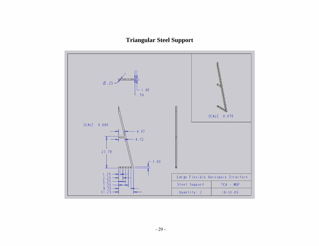
Triangular Steel Support

- 29 -

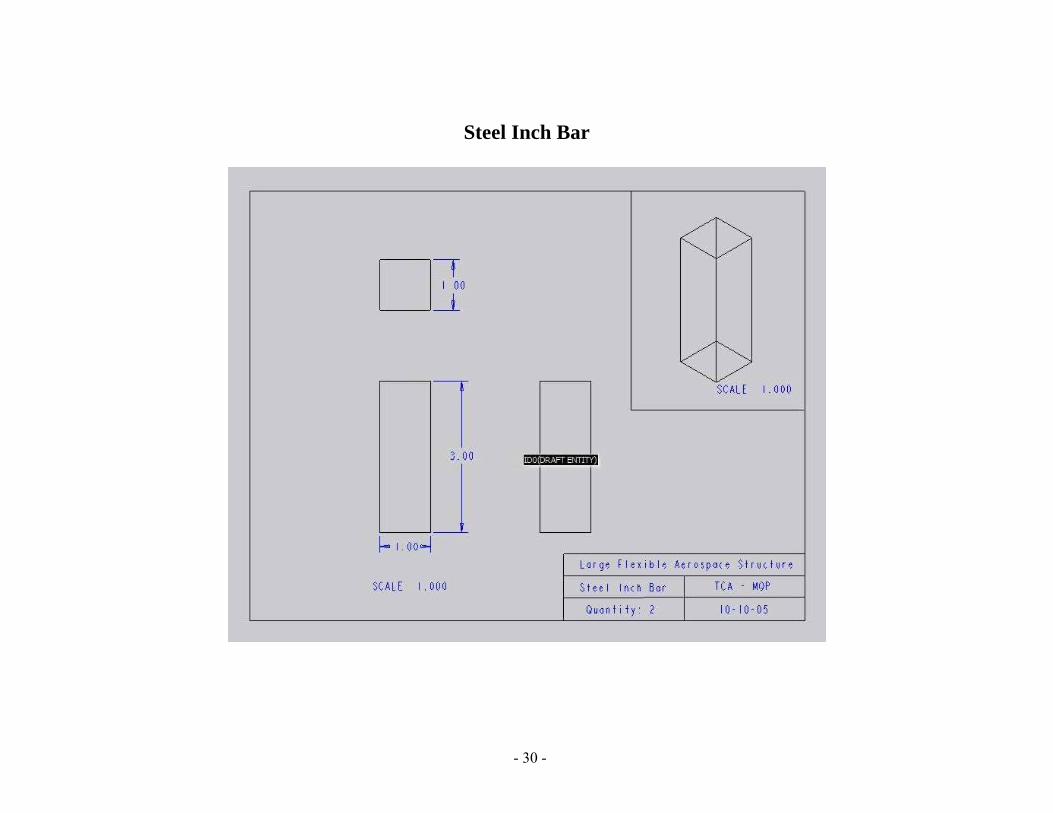
Steel Inch Bar

- 30 -

Steel Support Bar

- 31 -

- 32 -

Final Assembly

Appendix B: Table of Equipment

EQUIPMENT PRODUCER MODEL NO.

Optical Table Technical Manufacturing Corperation (TMC) 78-23765-01

Amplifier Comdyna GP-6 PPC Controller Board D Space CLP 1103

PZT Quickpack Strain Actuator ACX QP20N

Signal Filter Krohn-Hite Model 3364

Operational Amplifier Comdyna GP-6 Function Generator Instek GFG-8219A

EQUIPMENT PRODUCER/SUPPLIER MODEL NO.

10-18 Cold Rolled Steel Yarde Metals NA

60-61 T6 Aluminum Yarde Metals NA

Vacuum Pump and Compressor Edwards ED65

C-Clamps

Hydraulic Sheer UNK UNK

Drill Press with 90° Champer Tool Arboga-Wilton A3008W

Abrasive Hand Cutter with an 8" wheel DoAll NA

Belt Sander Hammond PD-10

Vertical Band Saw DoAll ML

Vertical Mill DoAll CNS-C-112

CV-DC Arc Welder, Power Source and Wire Feeder Miller

Millermatic 250

Horizontal Band Saw JET 414459

- 33 -

Appendix C: MatLab FFT Analysis Code

close all load('C:\Documents and Settings\acrobot\Desktop\Large Space Structure MQP\FFT Analysis\sensor1.txt') load('C:\Documents and Settings\acrobot\Desktop\Large Space Structure MQP\FFT Analysis\sensor2.txt') load('C:\Documents and Settings\acrobot\Desktop\Large Space Structure MQP\FFT Analysis\sensor3.txt') load('C:\Documents and Settings\acrobot\Desktop\Large Space Structure MQP\FFT Analysis\sensor4.txt') load('C:\Documents and Settings\acrobot\Desktop\Large Space Structure MQP\FFT Analysis\accelerometer.txt') delta_t=0.001; t_len=20; HF=1/(2*delta_t); HL=1/(2*t_len); f=HL:(HF-HL)/(length(sensor1)-1):HF; length (f) Y=fft(sensor1); Pyy1 = Y.* conj(Y); figure(1) loglog(f,Pyy1) Y=fft(sensor2); Pyy2 = Y.* conj(Y); figure(2) loglog(f,Pyy2) Y=fft(sensor3); Pyy3 = Y.* conj(Y); figure(3) loglog(f,Pyy3) Y=fft(sensor4); Pyy4 = Y.* conj(Y); figure(4) loglog(f,Pyy4) Y=fft(accelerometer); Pyy5 = Y.* conj(Y); figure(5) loglog(f,Pyy5)

- 34 -

References

[1] Allen, Robert, ed. New Materials: Building Structures in Space. NASA. Comp. Brian Dunbar. Aug. 1996. NASA. Sept.-Oct. 2005 <http://www.nasa.gov/centers/langley/news/factsheets/Bldg-structures.html>. [2] Allen, Robert, ed. Middeck Active Control Experiment: Building Structures in Space. NASA. Comp. Brian Dunbar. Aug. 1996. NASA. Sept.-Oct. 2005 <http://www.nasa.gov/centers/langley/news/factsheets/Bldg-structures.html>. [3] Johnson, Conor, and Keith K Denoyer. Recent Achievements in Vibration Isolation. Vers. IAF-01-I.2.01. Oct. 2001. CSA Engineering Inc. Sept.-Oct. <http://http://www.csaengineering.com/techpapers/technicalpaperpdfs/CSA2001Launch_onorbit.pdf>. [4] Serway and Beichner. Physics for Scientists and Engineers. Thopson Learning, 2000. 409-412. [5] Preumont, Andre. Vibration and Control of Active Structures. The Netherlands: Kluwer Academic, 1997. pp (35-36). [6] Preumont, Andre. Vibration and Control of Active Structures. The Netherlands: Kluwer Academic, 1997. pp(40-42). [7] Preumont, Andre. Vibration and Control of Active Structures. The Netherlands: Kluwer Academic, 1997. p(4). [8] Moheimani, S.o. Reza, ed. An optimization approach to optimal placement. 18 Nov. 2000. University of Newcastle, Australia. Sept.-Oct. <http://rumi.newcastle.edu.au/reza/PAPERS/opt_placement.pdf>. [9] Blevins, Robert D. Formulas for Natural Frequency and Mode Shape. Malabar, FL: Krieger Company, 2001. 233. [10] TMC 63-500 Laboratory Tables. 2005. 12 Oct. 2005 <http://www.techmfg.com/products/labtables/63500.htm>. [11] Blevins, Robert D. Formulas for Natural Frequency and Mode Shape. Malabar, FL: Krieger Company, 2001. 261. [12] Demetriou, Michael, and Raffaele Potami. Scheduling policies of intelligent sensors and sensor/actuators in flexible structures. Worcester Polytechnic Institute, 2005.

- 35 -