Design and Sample Size for SMART Studies

See discussions, stats, and author profiles for this publication at: https://www.researchgate.net/publication/328583753

Design and Sample Size Calculation for SMART Studies

Presentation · November 2016

DOI: 10.13140/RG.2.2.13901.90085

CITATIONS

0READS

188

11 authors, including:

Some of the authors of this publication are also working on these related projects:

Evaluation of Diabetic Retinal Screening and Factors for Ophthalmology Referral in a Telemedicine Network View project

Causes and Prevalence of Anemia in Hereditary Hemorrhagic Telangiectasia View project

Michael R Kosorok

University of North Carolina at Chapel Hill

248 PUBLICATIONS 7,395 CITATIONS

SEE PROFILE

Arkopal Choudhury


7 PUBLICATIONS 35 CITATIONS

SEE PROFILE

Yifan Cui


10 PUBLICATIONS 15 CITATIONS

SEE PROFILE

Eric Laber

North Carolina State University

54 PUBLICATIONS 1,239 CITATIONS

SEE PROFILE

All content following this page was uploaded by Arkopal Choudhury on 29 October 2018.

The user has requested enhancement of the downloaded file.

https://www.researchgate.net/publication/328583753_Design_and_Sample_Size_Calculation_for_SMART_Studies?enrichId=rgreq-43d5781b5e4efacd8c277ab5a1531e53-XXX&enrichSource=Y292ZXJQYWdlOzMyODU4Mzc1MztBUzo2ODcxNzcxNTEyOTk1ODVAMTU0MDg0NzIwODM5OA%3D%3D&el=1_x_2&_esc=publicationCoverPdf

https://www.researchgate.net/publication/328583753_Design_and_Sample_Size_Calculation_for_SMART_Studies?enrichId=rgreq-43d5781b5e4efacd8c277ab5a1531e53-XXX&enrichSource=Y292ZXJQYWdlOzMyODU4Mzc1MztBUzo2ODcxNzcxNTEyOTk1ODVAMTU0MDg0NzIwODM5OA%3D%3D&el=1_x_3&_esc=publicationCoverPdf

https://www.researchgate.net/project/Evaluation-of-Diabetic-Retinal-Screening-and-Factors-for-Ophthalmology-Referral-in-a-Telemedicine-Network?enrichId=rgreq-43d5781b5e4efacd8c277ab5a1531e53-XXX&enrichSource=Y292ZXJQYWdlOzMyODU4Mzc1MztBUzo2ODcxNzcxNTEyOTk1ODVAMTU0MDg0NzIwODM5OA%3D%3D&el=1_x_9&_esc=publicationCoverPdf

https://www.researchgate.net/project/Causes-and-Prevalence-of-Anemia-in-Hereditary-Hemorrhagic-Telangiectasia?enrichId=rgreq-43d5781b5e4efacd8c277ab5a1531e53-XXX&enrichSource=Y292ZXJQYWdlOzMyODU4Mzc1MztBUzo2ODcxNzcxNTEyOTk1ODVAMTU0MDg0NzIwODM5OA%3D%3D&el=1_x_9&_esc=publicationCoverPdf

https://www.researchgate.net/?enrichId=rgreq-43d5781b5e4efacd8c277ab5a1531e53-XXX&enrichSource=Y292ZXJQYWdlOzMyODU4Mzc1MztBUzo2ODcxNzcxNTEyOTk1ODVAMTU0MDg0NzIwODM5OA%3D%3D&el=1_x_1&_esc=publicationCoverPdf

https://www.researchgate.net/profile/Michael_Kosorok?enrichId=rgreq-43d5781b5e4efacd8c277ab5a1531e53-XXX&enrichSource=Y292ZXJQYWdlOzMyODU4Mzc1MztBUzo2ODcxNzcxNTEyOTk1ODVAMTU0MDg0NzIwODM5OA%3D%3D&el=1_x_4&_esc=publicationCoverPdf


https://www.researchgate.net/institution/University_of_North_Carolina_at_Chapel_Hill?enrichId=rgreq-43d5781b5e4efacd8c277ab5a1531e53-XXX&enrichSource=Y292ZXJQYWdlOzMyODU4Mzc1MztBUzo2ODcxNzcxNTEyOTk1ODVAMTU0MDg0NzIwODM5OA%3D%3D&el=1_x_6&_esc=publicationCoverPdf


https://www.researchgate.net/profile/Arkopal_Choudhury?enrichId=rgreq-43d5781b5e4efacd8c277ab5a1531e53-XXX&enrichSource=Y292ZXJQYWdlOzMyODU4Mzc1MztBUzo2ODcxNzcxNTEyOTk1ODVAMTU0MDg0NzIwODM5OA%3D%3D&el=1_x_4&_esc=publicationCoverPdf




https://www.researchgate.net/profile/Yifan_Cui?enrichId=rgreq-43d5781b5e4efacd8c277ab5a1531e53-XXX&enrichSource=Y292ZXJQYWdlOzMyODU4Mzc1MztBUzo2ODcxNzcxNTEyOTk1ODVAMTU0MDg0NzIwODM5OA%3D%3D&el=1_x_4&_esc=publicationCoverPdf




https://www.researchgate.net/profile/Eric_Laber?enrichId=rgreq-43d5781b5e4efacd8c277ab5a1531e53-XXX&enrichSource=Y292ZXJQYWdlOzMyODU4Mzc1MztBUzo2ODcxNzcxNTEyOTk1ODVAMTU0MDg0NzIwODM5OA%3D%3D&el=1_x_4&_esc=publicationCoverPdf


https://www.researchgate.net/institution/North_Carolina_State_University?enrichId=rgreq-43d5781b5e4efacd8c277ab5a1531e53-XXX&enrichSource=Y292ZXJQYWdlOzMyODU4Mzc1MztBUzo2ODcxNzcxNTEyOTk1ODVAMTU0MDg0NzIwODM5OA%3D%3D&el=1_x_6&_esc=publicationCoverPdf



Design and Sample Size for SMART Studies

M. Kosorok, J. Chen, M. Chaudhari, A. Choudhury, Y. Cui, X. Jiang,M. Lawson, D. Luckett, C. Nguyen, T. Pokaprakarn, E. Laber

Department of BiostatisticsUniversity of North Carolina at Chapel Hill

11/17/2016

Kosorok et al. (UNC BIOS) SMART Design Workshop 11/17/2016 1 / 62

Outline

1 Precision medicine and dynamic treatment regimes

2 SMART study designs

3 Standard analysis methods and Q-learning

4 Sample size calculations

5 Preparing protocols

6 Advanced analysis methods


Precision Medicine

• Personalized approach rather than “one size fits all”

• Patients may exhibit heterogeneity in response to treatment

• Using patient information to assign treatment may improve outcomeswhile reducing cost and patient burden

• “The right treatment for each patient at the right time”


Personalized vs. Precision Medicine

• Personalized medicine:

• Tailored treatment that accounts for patient heterogeneity

• Not really new: clinicians have been doing this for years

• Precision medicine:

• Tailored treatment that is data-driven and reproducible

• Increasing and active area


Dynamic Treatment Regimes

A dynamic treatment regime (DTR) formalizes precision medicine as asequence of decision rules assigning treatment based on patient covariates.

• Example of a single-stage decision rule for selecting an antidepressantfor patients with bipolar disorder:1

• Covariates used to make decisions are called “tailoring variables”1Wu et al., 2015Kosorok et al. (UNC BIOS) SMART Design Workshop 11/17/2016 5 / 62

Dynamic Treatment Regimes (continued)

• A DTR consists of one decision rule per stage of intervention

• An optimal DTR maximizes the mean of some clinical outcome whenapplied to a population

• Estimating the optimal DTR from data is of interest


Outline








A Clinical Trial Design for Estimating the Optimal DTR

Early work involved estimating the optimal DTR from observational data.2

• Treatments are not randomized

• May be unmeasured confounders

This led to the development of a clinical trial design to generate data forestimating optimal dynamic treatment regimes: the sequential multipleassignment randomized trial (SMART).

2Robins, 2004Kosorok et al. (UNC BIOS) SMART Design Workshop 11/17/2016 8 / 62

Motivating Example: Pediatric Anxiety Disorder

• This example comes from Almirall et al. (2012)

• Treatments: sertraline (SERT) or cognitive behavioral therapy (CBT)

• Response assessed using scales for anxiety symptom severity

• Primary aims:

• Determine whether SERT or CBT is the better first line therapy

• Determine the best sequence of first and second line therapyaccounting for response to first line therapy

• Estimate an optimal DTR


An Example of a SMART


Introduction to SMART Designs

• Randomize treatment assignment at each decision time

• Collect baseline and interim patient information

• Primary outcome is often observed after last decision time

• Allows for:

• Comparing outcomes under different first line treatments

• Comparing outcomes under different fixed sequences of treatments

• Estimating optimal DTR’s


Delayed Effects

An example: alcohol addiction management.3

• Available first line treatments: Naltrexone with low-level counseling(NTX) or combined behavioral intervention (CBI)

• Second line treatment for responders to first line treatment:telephone monitoring (TEL) or telephone counseling and monitoring(TEL + Counseling)

• CBI appears to have no benefit over NTX after first line treatment

• Patients who received CBI respond better after TEL + Counseling

• CBI teaches patients how to utilize counseling; benefit is not seenuntil after second line treatment

3Murphy, 2005Kosorok et al. (UNC BIOS) SMART Design Workshop 11/17/2016 12 / 62

Alcohol Addiction Management


Choosing an Alcohol Addiction Treatment Regime

• There are eight possible regimes

• Combining RCT’s to select the best regime:

• Conduct a two-arm trial of NTX vs. CBI and select the best

• Conduct a follow-up trial that assigns the best initial treatment andthen randomizes to second line treatment based on response

• Based on the follow-up study, select the best second line treatment

• This approach doesn’t account for delayed effects


Illustration of Delayed Effects

• Red boxes contain mean days abstinent in six months

• NTX yields better immediate outcomes after six months


Illustration of Delayed Effects (continued)

• Best regime using naive approach: Assign NTX initially and thenassign step-up for non-responders and TEL for responders

• Assuming that 50% of patients respond, this regime results in anaverage of 33.75% days abstinent over one year


Illustration of Delayed Effects (continued)

• Optimal regime: CBI followed by TEL + Counseling for respondersand step-up treatment for non-responders

• Assuming 50% of patients respond, this regime results in an averageof 35.25% days abstinent, compared with 33.75% on the naive regime


Discussion of Delayed Effects

Delayed effects can be positive or negative:

• Positive synergies: treatment doesn’t initially appear effective but hasa long term effect when followed by a second treatment

• Negative synergies: treatment may produce an immediate responsebut side effects reduce the effect of subsequent treatments


Reasons to Use a SMART Instead of Combining RCT’s

• Singe-stage RCT’s don’t allow for observing delayed effects

• Diagnostic effects: a treatment may not be effective but may revealsymptoms that help us to choose better subsequent treatment

• Patients may be more likely to remain in the study if they knowtreatment may be switched if they don’t respond


SMART Design Considerations

Domain knowledge should dictate:

• Time between randomizations

• Whether or not to randomize based on response status

• Set of treatments available at each stage

• Outcomes used to assess response

Sequences of treatments given in a SMART should be among those thatwould be considered in clinical practice.


Possible Aims of a SMART

• Compare response among initial treatments

• Intent-to-treat comparison of initial treatments

• Determine the best sequence of treatments

• Estimate optimal DTR’s

• Many other possibilities


Example Aim: Comparison of Initial Treatments


Comparison of Initial Treatments (continued)

• Reduces to a standard RCT

• Standard analysis methods can be used:

• Compare mean outcomes between two initial treatments using a t-test

• Compare mean outcomes across more than two initial treatments

• Adjust for covariates using linear regression

• Standard sample size calculations apply


Example Aim: Intent-to-treat Comparison of InitialTreatments


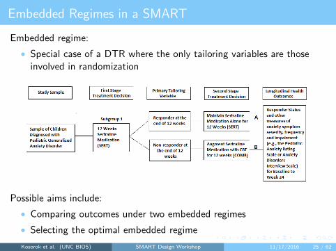
Embedded Regimes in a SMART

Embedded regime:

• Special case of a DTR where the only tailoring variables are thoseinvolved in randomization

Possible aims include:

• Comparing outcomes under two embedded regimes

• Selecting the optimal embedded regime


Examples of Embedded Regimes


Outline








Linear Regression for SMART’s

The linear regression model takes the form

Y = β0 +Xᵀβ1 +Aβ2 + ε,

where

• Y denotes response to initial treatment (anxiety symptom severity)

• X denotes baseline covariates

• A denotes initial treatment (A = 1 for SERT and A = 0 for CBT)

Testing H0 : β2 = 0 is a comparison of initial treatment while adjusting forcovariates. Different types of outcomes can be accounted for using GLM’s.


Potential Outcomes

In a clinical application involving only one decision:

• Covariates X ∈ X ⊆ Rp; treatment A ∈ A; outcome Y ∈ R

• Assume that larger values of Y are better

• Define Y ∗(a) to be the potential outcome under treatment a

• Assumptions to connect potential outcomes with the observed data:

1 Consistency: Y = Y ∗(A)

2 Positivity: Pr(A = a|X = x) ≥ c for some c > 0 and all pairs (x, a)

3 Strong ignorability: Y ∗(a)⊥A|X for all a ∈ A

• Assumptions 2 and 3 are satisfied by design in a SMART


Single-stage Decision Making

• A decision rule for treatment is a map d : X → A such that a patientpresenting with covariates x will be assigned treatment d(x)

• Define the Q-function by Q(x, a) = E {Y ∗(a)|X = x,A = a}

• Under the assumptions on the previous slide,

Q(x, a) = E (Y |X = x,A = a)

• The optimal decision rule at x is dopt(x) = maxa∈AQ(x, a)


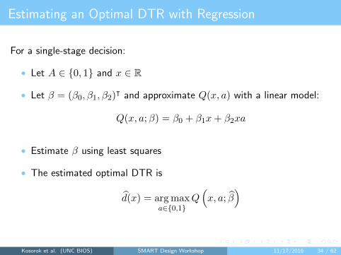
Estimating an Optimal DTR with Regression

For a single-stage decision:

• Let A ∈ {0, 1} and x ∈ R

• Let β = (β0, β1, β2)ᵀ and approximate Q(x, a) with a linear model:

Q(x, a;β) = β0 + β1x+ β2xa

• Estimate β using least squares

• The estimated optimal DTR is

d(x) = argmaxa∈{0,1}

Q(x, a; β

)


Introduction to Q-learning

The estimation on the previous slide is a special case of Q-learning:

• A technique involving a sequence of recursive regressions to model therelationship between treatment and outcome conditional on covariatesand select treatment to optimize expected outcome given covariates

• A reinforcement learning method adapted from computer science

• Recursive nature accounts for delayed effects

• Conceptually straightforward, easy to implement, and easy to explainto collaborators


Multi-stage Decision Making

Many clinical areas require sequential treatments:

• T decision time points

• Covariates Xt ∈ Xt ⊆ Rp, t = 1, . . . , T collected between time t− 1and time t

• Treatment At ∈ At, t = 1, . . . , T taken at time t

• Outcome Y ∈ R observed after treatment AT

• Let Ht = (X1, A1, X2, . . . , Xt) be all information available at thetime of selecting At, called the “history”


Potential Outcomes in Multiple Stages

• Let aT = (a1, . . . , aT ) be a sequence of treatments

• Define the sequence of potential outcomes under aT by

X∗(aT ) = {X1, X∗2 (a1), . . . , X

∗T (aT−1)}

• Define Y ∗(aT ) to be the potential response under aT

• Assumptions to connect potential outcomes with the observed data:

1 Consistency: X∗t (at−1) = Xt for all t = 1, . . . , T and Y = Y ∗(aT )

2 Positivity: There exists c > 0 such that Pr(At = at|Ht = ht) ≥ c forall t = 1, . . . , T and all pairs (ht, at)

3 Sequential ignorability: At⊥X∗(aT )|Xt for all sequences aT

• Assumptions 2 and 3 are satisfied by design in a SMART


Q-learning

Recall a DTR is a sequence of decision rules:

• Let d = (d1, . . . , dT ) where dt : Xt → At

• Define the Q-function at time t by

Qt(ht, at) = E(Y |Ht = ht, At = at)

• The optimal decision at time t is doptt (ht) = maxat∈At Qt(ht, at)

• The optimal DTR is dopt = (dopt1 , . . . , doptT )

• Goal: Use observed data to estimate dopt


Q-learning (continued)

Basic idea: Use observed data to recursively estimate the Q-functions andinfer optimal decisions based on estimated Q-functions. For T = 2:

1 Postulate a model Q2(h2, a2;β2) = E(Y |h2, a2;β2)

2 Use the observed outcomes Yi, i = 1, . . . , n to estimate β2; denotethe estimated Q-function by Q2(h2, a2) = Q2(h2, a2; β2)

3 Compute the pseudo-outcomes Y = maxa2∈A2 Q2(h2, a2)

4 Postulate a model Q1(h1, a1;β1) and use pseudo-outcomes as theresponse in a regression to estimate β1

5 The estimated DTR is d = (d1, d2) where, for t = 1, 2,

dt(ht) = argmaxat∈At

Qt(ht, at).


Discussion of Q-learning

Advantages:

• Conceptually simple and easy to implement

• Based on regression models which are well-understood and easy toexplain to collaborators

Disadvantages:

• Requires specification of a model for the Q-function

• Can perform poorly under a misspecified model

Instead of linear regression, try random forests or support vector regressionto estimate the Q-function.


Outline








Comparing Two Embedded Regimes

Let d1 and d2 be two embedded regimes in a SMART. Let µd1 and µd2 bethe mean outcomes for patients who follow d1 and d2, respectively. Wewant to test

H0 : µd1 = µd2 vs. H1 : µd1 6= µd2 .

Weight each patient by the inverse probability of receiving the treatmentthey did. Let Wi be the weight and let Nd be the number of patientswhose treatment paths were consistent with d. An estimator for µd is

Y d =

∑Ndi=1WiYi∑Ndi=1Wi

,

which forms the basis for a test statistic.4

4Ghosh et al., 2015Kosorok et al. (UNC BIOS) SMART Design Workshop 11/17/2016 42 / 62

Sample Size for Comparing Embedded Regimes

We need to use inverse probability weighting. In the following simpleexample, Wi = 2 for responders and Wi = 4 for non-responders.


Sample Size for Comparing Regimes (continued)

When the outcome, Y , is continuous:

• Consider a size α two-sided test of

H0 : µd1 = µd2 H1 : µd1 6= µd2

for embedded regimes d1 and d2 with different initial treatments

• Let γ1, γ2 ∈ (0, 1) be the response rates to initial treatments

• Let σ2 = Var(Y ) under d1 and d2

• To have power 1− β when µd1 − µd2 = δ we need5

N = 2(zα/2 + zβ)2(4− γ1 − γ2)

1

(δ/σ)2

• Straightforward extensions to binary outcomes and unknown variance

5Ghosh et al., 2015Kosorok et al. (UNC BIOS) SMART Design Workshop 11/17/2016 44 / 62

Sample Size for Finding the Optimal Embedded Regime

• Assume d1 is the optimal embedded regime, i.e., µd1 ≥ µdj + δ forsome δ > 0 and all j 6= 1

• We can calculate the sample size such that

Pr(Y d1 − Y d2 > 0, . . . , Y d1 − Y dJ > 0

)≥ 1− β,

where J is the number of embedded regimes in our SMART

• Use Bonferroni correction: calculate the sample size such that

Pr(Y d1 − Y dj > 0

)≥ 1− βj , j = 2, . . . , J

and 1− β =∑J

j=2(1− βj), for example βj = β/(J − 1)

• Much smaller sample sizes than traditional hypothesis testing


Sample Size for Estimating an Optimal DTR

Little work has been done in sizing a trial for estimating an optimal DTR.

• Sample sizes can be calculated by inverting a plug-in projectionconfidence interval for the expected outcome under a given DTR6

• Requires data from a small pilot study

• In a single-stage setting, let V (d) = E {Y |A = d(X)}. The goal is tochoose n such that:

• The power to reject H0 : V (dopt) = V0 in favor of H1 : V (dopt) > V0is at least 1− β when V (dopt) ≥ (1 + δ)V0 for some δ

• Pr{∣∣∣V (d)− V (dopt)

∣∣∣ ≤ ε} ≥ 1− β,

where β and ε are specified by the user

6Laber et al., 2016Kosorok et al. (UNC BIOS) SMART Design Workshop 11/17/2016 46 / 62

Sample Size by Simulation

Another option is calculating sample size using simulation.

• Estimate expected outcome under the estimated optimal DTR for avariety of sample sizes

• Choose the smallest sample size with acceptable estimated outcome

6Zhao et al., 2011Kosorok et al. (UNC BIOS) SMART Design Workshop 11/17/2016 47 / 62

Outline








Difficulties in Data Collection and Management

Protocol should address data collection and management:

• Collection across multiple clinical sites may lead to accuracy problems

• Ease of data access and privacy need to be considered

• Randomization may create data mangament issues

• Data flow diagram can be used to map the data collection,processing, storage, and security


Challenges with Preparing Protocols

General challenges when submitting a SMART grant proposal:

• Need for increased communication between statisticians and clinicianswhen designing study and preparing protocol

• Nonstandard sample size calculations

• Reviewers may be unfamiliar with SMART designs

• Reviewers may be unfamiliar with novel statistical methods


Responding to Reviewer Comments

Sample comments:

• “The design deviates from the standard SMART design byre-randomizing all subjects after 6 months. It’s unclear how theproposed analysis methods will work in this setting.”

• “The hypothesis being tested - that of selecting the best treatment -can be tested with a usual RCT. Why invest the time and money in aSMART trial?”

• “The trial is sized for finding the optimal embedded regime but type Ierror is not mentioned. How does the trial account for type I error?”

How can we effectively respond?


Recommendations for Preparing Protocols

• Clearly define research goals – why is a SMART needed?

• Carefully justify each aspect of study design

• Set of treatment options

• Set of tailoring variables

• Decision time points

• Include standard analysis methods that reviewers will understand

• Emphasize advantages of SMART’s:

• Why is a SMART design best for your research question?

• Why is a SMART design novel in your research area?

• What does a SMART give you that another design would not?


Recommendations for Preparing Protocols (continued)

Sample language for a protocol:

• “Analyses for aim 1 require estimating a personalized, adaptiveintervention. Using data from this SMART, we will use Q-learning toestimate an adaptive intervention strategy to maximize patientoutcome at the end of follow-up.”

• “For aim 1, we will use Q-learning with linear models to estimatedynamic treatment regimes to maximize patient outcome. Areinforcement learning method, Q-learning is a technique forsequential decision-making that involves estimating the relationshipbetween an outcome and a series of actions and choosing actions thatlead to the most desirable outcome.”


Outline








Advanced Methods: Interactive Q-learning

Recall basic Q-learning with linear models:

1 Regress Y on H2, A2: Q2(H2, A2) = βᵀ21H2 + βᵀ22H2A2

2 Compute the pseudo-values

Y = βᵀ21H2 + maxa2∈{1,−1}

βᵀ22H2a2 = βᵀ21H2 + |βT22H2|


IQ-learning: regression takes place before non-smooth maximization.


2 Model E(|βᵀ22H2| |H1, A1) =∫|z|f(z|H1, A1)dz

3 Regress βᵀ21H2 on H1, A1

4 Combine the two previous steps to get Q1(H1, A1)


BOWL (Backward OWL)

Idea: directly target mean outcome under a given DTR.7

• Two stages with outcomes Y1 and Y2 and treatments A1 and A2

• Assuming Pr(A1 = 1|H) = Pr(A2 = 1|H) = 1/2,

E {Y1 + Y2|A1 = d1(H1), A2 = d2(H2)} =4E[(Y1 + Y2)1 {A1 = d1(H1)} 1 {A2 = d2(H2)}]

• Obtain d2 by minimizing an approximation of En [Y21 {A2 6= d2(H2)}]

• Obtain d1 by minimizing an approximation of

En[(Y1 + Y2)1

{A2 = d2(H2)

}1{A1 6= d1(H1)

}]• Surrogate loss functions needed because of the indicator functions

7Zhao et al., 2015Kosorok et al. (UNC BIOS) SMART Design Workshop 11/17/2016 56 / 62

SOWL (Simultaneous OWL)

Idea: similar to BOWL, but optimization occurs in one step.8

• Assume T decision time points with outcome Yt observed at time t

• Maximize

En

(∑T

t=1 Yt

)∏Tt=1 1 {At = dt(Ht)}∏T

t=1 πt(At, Ht)

where πt(at, ht) = Pr(At = at|Ht = ht)

• Define a concave surrogate ψ(Z1, Z2) = min(Z1 − 1, Z2 − 1, 0) + 1

• The SOWL estimator is the maximizer of

En

[(∑T

t=1 Yt)ψ {A1f1(H1), A2f2(H2)}∏Tt=1 πt(At, Ht)

],

over f1, f2, where dt(ht) = sign {ft(ht)}8Zhao et al., 2015Kosorok et al. (UNC BIOS) SMART Design Workshop 11/17/2016 57 / 62

Discussion of Advanced Methods

• IQ-learning:

• More robust to model misspecification than Q-learning

• Switching estimation and maximization makes efficient use of data

• BOWL:

• Transforms estimation of an optimal DTR into a classification problem

• Amount of data that is used decreases with each decision time

• SOWL:

• Doesn’t require multiple steps like BOWL


Other methods

Many other statistical methods are relevant to SMART’s:

• G-estimation (Stephens, 2015)

• Marginal structural models (Robins, 2004)

• A-learning (Murphy, 2003)


Conclusions

• Dynamic treatment regimes (DTR’s) have the potential to improvepatient outcomes while reducing cost and burden of treatment

• SMART’s provide a clinical trial design for estimating optimal DTR’s

• A SMART can also be used to make primary comparisons betweentreatments and can be powered like an RCT

• Novel statistical methods and sample size calculations are needed

• Potential exists for statistical and biomedical research in this area


References

• Wu, F., Laber, E. B., Lipkovich, I. A., & Severus, E. (2015). Who will benefitfrom antidepressants in the acute treatment of bipolar depression? A reanalysis ofthe STEP-BD study by Sachs et al. 2007, using Q-learning. International journalof bipolar disorders, 3(1), 1-11.

• Robins, J. M. (2004). Optimal structural nested models for optimal sequentialdecisions. In Proceedings of the second seattle Symposium in Biostatistics(pp.189-326). Springer, New York.

• Almirall, D., Compton, S. N., GunlicksStoessel, M., Duan, N., & Murphy, S. A.(2012). Designing a pilot sequential multiple assignment randomized trial fordeveloping an adaptive treatment strategy. Statistics in medicine, 31(17),1887-1902.

• Murphy, S. A. (2005). An experimental design for the development of adaptivetreatment strategies. Statistics in medicine, 24(10), 1455-1481.

• Ghosh, P., Cheung, Y., & Chakraborty, B. (2015). Sample size calculations forclustered smart designs. Adaptive Treatment Strategies in Practice: PlanningTrials and Analyzing Data for Personalized Medicine, 55-70.


References (continued)

• Laber, E. B., Zhao, Y. Q., Regh, T., Davidian, M., Tsiatis, A., Stanford, J. B., ...& Kosorok, M. R. (2015). Using pilot data to size a twoarm randomized trial tofind a nearly optimal personalized treatment strategy. Statistics in medicine.

• Zhao, Y., Zeng, D., Socinski, M. A., & Kosorok, M. R. (2011). Reinforcementlearning strategies for clinical trials in nonsmall cell lung cancer. Biometrics, 67(4),1422-1433.

• Laber, E. B., Linn, K. A., & Stefanski, L. A. (2014). Interactive model building forQ-learning. Biometrika.

• Zhao, Y. Q., Zeng, D., Laber, E. B., & Kosorok, M. R. (2015). New statisticallearning methods for estimating optimal dynamic treatment regimes. Journal ofthe American Statistical Association, 110(510), 583-598.

• Stephens, D.A. (2015). G-estimation for dynamic treatment regimes in thelongitudinal setting. Adaptive Treatment Strategies in Practice: Planning Trialsand Analyzing Data for Personalized Medicine, 89-118.

• Murphy, S. A. (2003). Optimal dynamic treatment regimes. Journal of the RoyalStatistical Society: Series B (Statistical Methodology), 65(2), 331-355.

Kosorok et al. (UNC BIOS) SMART Design Workshop 11/17/2016 62 / 62View publication statsView publication stats

https://www.researchgate.net/publication/328583753

Design and Sample Size for SMART Studies

Documents

Transcript of Design and Sample Size for SMART Studies