Design and Prototyping of a High Country (HiCEV)
129
Design and Prototyping of a High Country Electric Vehicle (HiCEV) A thesis submitted in partial fulfilment of the requirements for the Degree of Masters of Engineering in Electronic and Electrical Engineering By Pierce L. Hennessy 2016
Transcript of Design and Prototyping of a High Country (HiCEV)

Design and Prototyping of a High Country Electric Vehicle (HiCEV)
A thesis submitted in partial fulfilment of the requirements for the Degree of Masters of Engineering in
Electronic and Electrical Engineering
By
Pierce L. Hennessy
2016

2
Abstract
The development of a High Country Electric Vehicle has come about in response to a farmers desire to
reduce the dependence on fossil fuels on his station. Electric vehicles have become more prominent in
the urban commuter vehicle market over recent years, and are gaining greater acceptance as people
look to be more environmentally aware. This project shows that electric vehicles also have a place in the
primary sectors in an off-roading, rugged context.
The conversion vehicle of choice is the Toyota Land Cruiser 70 Series, an iconic farming vehicle
renowned for its reliability in challenging operating conditions. The vehicle was stripped of components
associated with the 1-HZ internal combustion engine (ICE) drivetrain, and electrical drivetrains was
scoped, sourced and implemented in the vehicle.
This report investigates the systems integration aspects associated with modern electrical vehicle
components. The aspects of integration covered mechanical analysis of shaft coupling, interfacing
CANbus systems, high voltage system safety and low voltage wiring loom mapping. The vehicle has
reached self-propulsion and validation testing against the initial vehicle modeling is underway.

3
Acknowledgements
I would like to thank my supervisor Dr Paul Gaynor for his continued support and faith in me and John
Shrimpton for his unbounded enthusiasm and foresight to initiate the HiCEV project. Thank you to the
technical staff of Canterbury University for your support in locating the vehicle and providing expertise
and guidance. Also, thank you to the student groups I have had the pleasure of working with over the
last couple of years, you have made HiCEV what it is today.
To Jeff and the Brown family – I cannot thank you enough for the time you have given to me and this
project, to say you were generous falls far short of the mark. Your technical expertise and hands on
knowledge was critical in forming HiCEV.
Finally thanks to all my friends and family for your undying support, especially when things went pear
shaped. There is no chance I would have made this voyage without you.

4
Table of Contents 1.0 Introduction ...............................................................................................................................8
1.1 Project Motivation ........................................................................................................................ 8
1.1.1 Location ........................................................................................................................................ 8
1.2 Electric Vehicles in NZ ................................................................................................................... 9
1.3 Sustainability in NZ Transportation............................................................................................. 10
2.0 Background .............................................................................................................................. 10
2.1 Emissions ........................................................................................................................................... 11
2.1 Electrical Principals ..................................................................................................................... 11
2.1.1 Electrical Terminology ................................................................................................................ 11
2.1.2 Motor Theory ............................................................................................................................. 12
2.1.2.1 DC Motors ........................................................................................................................... 12
2.1.2.2 Induction Motors ................................................................................................................ 13
2.1.2.3 BLDC / PMAC Motors .......................................................................................................... 14
2.1.2.4 Motor Losses and Cooling ................................................................................................... 16
2.1.3 Inverter Theory .......................................................................................................................... 17
2.1.3.1 Field Orientated Control (FOC) ........................................................................................... 18
2.1.4 CANbus Communication ............................................................................................................ 18
2.1.4.1 CANbus in Automotive ........................................................................................................ 18
2.1.4.2 CAN Terminology ................................................................................................................ 18
2.1.4.3 CAN Operation .................................................................................................................... 19
2.1.5 Battery Theory ........................................................................................................................... 19
2.1.5.1 Battery Chemistries ............................................................................................................. 20
2.1.6.2 Shielding .............................................................................................................................. 23
2.1.6 Electro Magnetic Noise .............................................................................................................. 23
2.2. Vehicle Principals ............................................................................................................................. 24
2.2.1. Basic Theory of Operation ........................................................................................................ 24
2.2.2. EV Component Configurations .................................................................................................. 25
BEV .............................................................................................................................................. 25
HEV .............................................................................................................................................. 25
REEV ............................................................................................................................................ 25
FCEV ............................................................................................................................................ 25
2.2.3. Drivetrain Typologies ................................................................................................................ 25

5
2.3. Role of Systems Engineer ................................................................................................................. 25
3.0 Prototype Specification Design.................................................................................................. 27
3.1. Stakeholder Requirements ......................................................................................................... 27
3.1.1. Costings ............................................................................................................................... 27
3.2. User Requirements ..................................................................................................................... 27
3.2.1. Client and Intended use ...................................................................................................... 27
3.2.2. Donor Vehicle ...................................................................................................................... 28
3.2.3. Off-Road Operation ............................................................................................................. 28
3.2.4. Performance and Drivetrain ............................................................................................... 29
3.2.4.1. Typology ...................................................................................................................... 30
3.3. System Requirements ................................................................................................................. 31
3.3.1. Vehicle Performance ........................................................................................................... 31
3.3.1.1. HiCEV Estimated Characteristics ................................................................................. 31
3.3.1.2. Regenerative Braking and Range Extension ............................................................... 33
3.4. Component Sourcing .................................................................................................................. 34
3.4.1. Motor and Inverter combination ........................................................................................ 34
3.4.1.1. Motor Selection .......................................................................................................... 36
3.4.1.2. Inverter Selection ........................................................................................................ 37
3.4.2. Remaining Main Components ............................................................................................. 39
3.4.2.1. Battery Pack Sizing ...................................................................................................... 39
3.4.2.2. Remaining main system modules ............................................................................... 45
3.5. Main Architectural Design .......................................................................................................... 50
3.5.1. Component Layout .............................................................................................................. 51
3.5.2. Electrical Layout .................................................................................................................. 53
3.5.3. Mechanical Layout .............................................................................................................. 54
3.5.3.1. Motor to drivetrain ..................................................................................................... 54
3.5.3.2. Battery Boxes .............................................................................................................. 59
3.1 Subsystem Development ............................................................................................................ 61
3.1.1 Thermal Systems ................................................................................................................. 62
3.1.2 Motor Cooling ..................................................................................................................... 63
3.1.3 Inverter Cooling................................................................................................................... 66
3.1.4 Charger Cooling ................................................................................................................... 68
3.1.5 Power Steering .................................................................................................................... 68

6
3.1.6 Dash Cluster ........................................................................................................................ 68
3.1.7 Change Over switching unit ................................................................................................ 68
4.0 Testing and Commissioning ....................................................................................................... 68
4.1 Main Modules ............................................................................................................................. 68
4.2 Calibration ................................................................................................................................... 69
4.2.1 Electric Vehicle Control Module (EVCM) ............................................................................ 69
4.2.1.1. EVCM Hardware, Control and Implementation ................................................................. 71
4.2.2 Eltek Charger Calibration .................................................................................................... 81
4.2.3 BMS Calibration................................................................................................................... 85
4.2.4 Rinehart 150 DX inverter Settings ....................................................................................... 88
4.3 Commissioning (Systems integration) ........................................................................................ 93
4.3.1 Motor Mechanical Development ........................................................................................ 93
4.3.2 Inverter................................................................................................................................ 95
4.3.2.1 Interfacing with Remy HVH 250-115 PO ......................................................................... 96
4.3.2.2 Resolver ........................................................................................................................... 96
4.3.2.3 HV Safety Circuit ............................................................................................................. 99
4.3.3 CANbus .............................................................................................................................. 106
4.3.3.1 CANbus Database .......................................................................................................... 106
4.3.4 Battery Pack ...................................................................................................................... 107
4.3.4.1 Initial BMS Setup ........................................................................................................... 109
4.3.5 Vehicle Analysis ................................................................................................................. 110
4.3.6 Cooling .............................................................................................................................. 113
5.0 Discussion .............................................................................................................................. 115
5.1 Issues Faced .............................................................................................................................. 115
5.2 Future for HiCEV........................................................................................................................ 115
6.0 Conclusion .............................................................................................................................. 115
7.0 Appendix ................................................................................................................................ 116
7.1 Birds eye view of component layout .............................................................................................. 116
7.2 CAD model of battery boxes ........................................................................................................... 117
7.3 Rinehart Wiring Diagram ................................................................................................................ 118
7.4 Inverter Loom Mapping .................................................................................................................. 119
7.5 Motor Performance Diagrams ........................................................................................................ 123
7.6 Class D Specifications ...................................................................................................................... 124

7
8.0 Bibliography ........................................................................................................................... 126

8
1.0 Introduction As the demand for electric vehicles (EVs) increases on a global scale largely due to environmental and
economic issues, the phasing of electric propulsion systems into different sectors of the vehicle fleet is
inevitable. EVs initially found their niche in light urban commuters, but have recently breached into
sectors such as racing, long distance commuters and heavy machinery [1, 2, 3, 4, 5]. Tesla Motors has
played a major role in increasing the public perception of EVs, with their new model S luxury sedan. The
Model S, aside from being a luxury vehicle (capable of 253 mile range), is the fastest on road sedan EV or
ICE, with 691 electrical HP and capable of 3.1 second 0-60mph [2]. This move towards EVs has started
slow, and faced many challenges but momentum is building behind the EV movement as people become
faced with the realities of the issues associated with internal combustion engine (ICE) vehicles. Climate
change, oil scarcity combined the fact that the advance of electric propulsion technology to have a
desirable vehicle capable of exceeding (ICE) vehicles in performance, price and reduced emissions is
quickly coming to fruition.
1.1 Project Motivation The motivation project arose from the desire of a South Island, New Zealand farm to be more self-
sufficient whilst taking the lead with a new application for electric vehicles. Glenthorne Station resides
beside Lake Coleridge in the middle of the South Island, is taking the initiative to look into and create an
electric vehicle for daily farm use. This high country electric vehicle (HiCEV) uses the shell of a 70 Series
Land Cruiser, to retain the durability of a farm vehicle, while not losing any performance. This EV acts as
a prototype for the station, with hopes that- down the track, there will be many electric vehicles on the
station based on this platform.
Acting as an introduction for electric vehicles into NZ farming, the hope is that there will be a future
move towards more self-sustaining agricultural practices in NZ. The requirements for HiCEV were bound
initially by the desire to use newly available EV components and the restrictions imposed by the harsh
operating conditions.
1.1.1 Location Glenthorne station is the culmination of two high country stations, lower Ryton station
(now ‘Lower Glenthorne’) and the Glenthorne station (now ‘Upper Glenthorne’), whose name was
retained. Located off the northern shore of Lake Coleridge, Glenthorne station is the embodiment of
‘High Country Station’. Lower Glenthorne sits at approximately 560m and Upper Glenthorne at 810m
meters above sea level and covering 25000 hectares [6]. There are sections of Glenthorne so steep that
no pasture grows, and is uninhabitable by cattle, the typology is shown in figure [1]. A public gravel road

9
runs through the middle of Glenthorne, allowing access to various lakes around the property including
Lake Coleridge itself.
Figure 1 Map of Glenthorne Station [6]
The temperature variation is also an interesting parameter to take into account for vehicles on the
station, with temperatures that can reach -20oC can make for interesting issues for not only EV’s, but ICE
vehicles also. At these temperatures, coolant can freeze, oil and battery electrolyte can become viscous
and moisture can build in electrical enclosures through condensation.
1.2 Electric Vehicles in NZ The term Electric Vehicle is a blanket term to describe many types of drivetrain topologies but the two
main types are battery electric vehicles (BEV) and hybrid electric vehicles (HEV). BEV’s are electric
vehicles whose energy storage is wholly electric, in the form of a large capacity battery pack and
charged from external electricity supplies [7]. HEV’s have both an electric power drivetrain, but also a
combustion system that can be used as either a form of on-board battery charging or as an alternative
drive train depending on drivetrain typology [8]. HEV’s come in with a range of battery capacities, the
smallest of which don’t require external charging, as the internal system charges the battery pack
though the ICE acting as a generator, or energy recapture in the form of regenerative braking. Plug-in
HEVs (PHEVs) have a larger battery pack and allow short range travel on battery power alone.
Electric vehicles have made their way into the NZ market, but are still vastly outnumbered by ICE
vehicles in both number and advertising. NZ’s total light fleet comprises of 589 registered EV’s [9] and
8,861 HEVs as of December 2013 [10]. For the past 10 years, the total light vehicle fleet size in NZ has
consistently grown fairly consistently, with new vehicles in 2012 comprising 52% of the total travel done
in NZ (13% Commercial, 39% Passenger) and 92% of total travel by light vehicle travel [10]

10
Commercially available EV’s are only really available as new vehicles (0-5 years old) as first sales
mass EV’s to NZ public began in 2011 [7].
To increase the rate of integration of EVs into NZ a major component would be increasing infrastructure
to support the new generation of motoring. Options for charging a plugin EV are either; household wall
chargers or public charging stations, of which there are 74 public charging stations currently in NZ [9].
Currently, the most common way to charge an EV is at home [11]. With the evolution of the NZ grid
towards a ‘smart-grid’, integrating communication with the current power transmission, chargers should
be able to communicate with the grid for the best times to charge for price and also back-feed from
vehicle to grid (V2G), acting as a network of power supplies for grid stability [12].
This project could form the basis of shifting focus from EVs solely being thought of as light urban
commuter vehicles. Main economic NZ sectors associated with heavy work such as agriculture, mining
and forestry could start phasing in electric work vehicles with this project in mind. This has several
benefits, as these sectors are often associated with trading the environment for economics, by taking
EVs into their fleets they will improve their public image while reducing their carbon footprint.
1.3 Sustainability in NZ Transportation New Zealand already has a majority of renewable sources for power generation with only 30% of
generation produced by non-renewables sources [7] which is a good step in the direction towards
reducing greenhouse gas emissions and creating an environmentally sustainable future. In the transport
sector, the government has placed an exemption for light electric motor vehicles for road user chargers
(RUC’s) until 2020, to give the public some incentive to invest in EVs for public transportation [13].
Policies such as the above are crucial to phasing NZ towards a more sustainable environment. There are
going to be have to be more serious changes, in the near future in regards to the general environment.
Electric vehicles will play an essential role in any sustainability model that takes into account the future
of personal transportation, to reduce the fossil fuel usage and thus the greenhouse gas emissions.
Energy security will also play a major role in NZ’s energy sustainability model. Oil reserves are depleting
globally with time, moving towards an electrified fleet reduces the dependency on oil prices beyond our
control becomes less of an issue [7].
Personal transportation has grown to be an essential part of many peoples everyday life to go wherever
they want any time they choose. Sustaining this becomes essential in applications such as farming work,
where patrolling large areas or land is essential for the upkeep of the station. This factor requires
electric vehicles to have the capacity for long duration travel, even if the average distance traveled daily
in NZ is 40km [10] which isn’t quite there yet for readily available BEVs. That being said, R&D into newer
higher capacity batteries with a relatively low cost per kWh is being investigated thoroughly worldwide
currently to reduce this hindering factor for potential EV buyers [14].
2.0 Background Electric vehicles (EVs) are widely viewed as the vehicle of choice in an environmentally responsible
society. They are available for personal use (private sales) and are being incorporated into fleet
purchases [15]. It should not be surprising that they are also being considered in other areas previously
dominated by fossil fueled vehicles.

11
Historically, vehicle evolution has enabled the human race to expand, interconnect and grow at a rate
exponentially faster than would have been possible without them, but this has come hand in hand with
crippling effects on the global environment. One of the major contributing factors is combustion engine
emissions [16]. To enable the human race to progress, while reducing the environmental impact of
vehicles, the proposed solution by many is to phase in low-to-zero pollution emitting electric vehicles.
This EV drivetrain technology is becoming increasingly prevalent, starting mainly in the light vehicle
transportation sector, but also heavy machinery as efficiency and torque delivery characteristics become
more widely acknowledged. The aim of this section is to highlight the main characteristics of EVs, such
as their low ground-to-road emission values comparatively with ICE vehicles, but also the drivetrain
technology in terms of common componentry and vehicle analysis.
2.1 Emissions The ‘Greenhouse Effect’ is a naturally occurring effect whereby gases in the atmosphere act as a
blanket, keeping the earth warm. Without this effect, the earth would be 33oC lower than it is now, and
the life that we have now would not have been possible [17]. Ideal global temperature is under threat as
mankind has exaggerated Greenhouse Effect by producing large quantities of CO2 – vehicle emissions
are a major contributor. People are questioning the widespread use of fossil fuels and the danger posed
to life on earth as a consequence of this.
As of 2012, the Transport sector in New Zealand (NZ) currently contributes 20% of total greenhouse
emissions by sector, second only to the Agricultural Methane emissions at 32% [18] and the current fleet
of EVs in NZ have saved 277 tons of CO2 emissions [9].
2.1 Electrical Principals Electricity is a secondary form of energy, generated from either renewable sources, fossil fuels or
nuclear primary source, and is arguably the most usable form of energy due to its ease of manipulation,
transmission and storage [19]. Electrical energy is the driving force of most societies today, with the vast
majority of people around the world heavily reliant on it for daily use. Personal transport has relied on
electricity since its conception, including powering sub-systems and communication in ICE vehicles, and
now the driving force in EV’s and Hybrids.
2.1.1 Electrical Terminology A list of terminology is given below for reference:
Subscripts
DC – Direct Current
AC – Alternating Current
RMS – Root Mean Squared
p – Peak
a, b, c – Phases in AC
m - Mechanical
e - Electrical
t - Torque
s - Synchronous
heat

12
Parameters and Units
V - Voltage (Volts)
I - Current (Amps)
P - Power (Watts)
E - Back EMF (Volts)
B – Magnetic field strength (Tesla)
λ - Flux (Weber)
F - Force (Newton)
τ - Torque (Newton.meter)
Ө - Angle (radian)
ω - Angular Velocity (radian.second-1)
t - Time (second)
K - Constant
p – Pole Pairs
BLDC - Brushless DC
PMAC - Permanent Magnet AC
2.1.2 Motor Theory The core of an electric vehicle is the motor, transforming electrical energy into motive force. The electric
motor is a remarkable piece of engineering, perfect for vehicle use: it has high power density, it is robust
and it is capable of regenerative braking. In an ICE system modeled by the Otto cycle, approximately
20% of the energy from the hydrocarbon based fuel is converted to motive energy, with the remaining
80% lost as heat, with a theoretical maximum thermal efficiency of 35% [20].When the ICE system has to
slow down, brakes must be used which dissipate more kinetic energy as heat in the brake rotor. An
electric motor can act as a generator (regenerative braking) and feed energy back into the battery pack
to slow the vehicle, thus regaining some of the energy used to accelerate the vehicle.
Appropriate choice of motor for any application is crucial, and with many different electric motors
available in today’s market place, narrowing down to a specific motor can become difficult. Many
factors impact this choice: the mains ones being price, availability, load and compatibility. The motor
typologies discussed in this section have been narrowed down to those most often used in consumer
and hobbyist electric vehicles. Since each topology has unique features commonly associated with it, by
first having a sound understanding of motor operation the last two factors with regards to motor choice
above become much easier to assess.
2.1.2.1 DC Motors
DC motors are the simplest motor available for EV drive applications, and are not considered by larger
scale manufacturers, rather enthusiasts and hobbyists. DC brushed motors are relatively bulky, require
maintenance on the commutator brushes, can generate large amounts of EMI and are generally less
efficient than other motors. However, DC brushed motors often suit hobbyists, as their cost, along with
their associated components makes them the cheapest option for an electric vehicle conversion. Most
of the pitfalls for DC motors are often associated with their mechanical commutation - brushes
contribute to voltage drop in the system, leading to a reduced efficiency. EMI is generated from arcing
from the brushes on the commutator and since friction needs to occur for commutation to take place,
the brushes wear down and need to be replaced, with carbon build up in the motor/on the commutator
needing to be removed to prevent unwanted conduction [21].

13
2.1.2.2 Induction Motors
The simplest AC motor construction that is implemented in EV/HEV applications is the induction motor.
Although generally having a lower operating efficiency and lower torque density than BLDC/PMAC AC
motors, induction makes up for it with generally a more robust design and reduced cost. [8]
As with all AC motors, an inherent benefit is that the mechanical commutation of DC motors is not
required, thus reducing maintenance requirements significantly, while increasing efficiency by having no
brush voltage drop [22].
The construction of an induction motor consists of; a housing enclosure, a stator, a rotor, a mechanical
shaft, bearings, sensors (position and temperature) and cooling (fan or liquid). The main aim of the
housing enclosure is sealing the motor while providing structural support for the machine and ease of
mounting [23]. The housing specification of a motor is crucial in some applications, such as those where
water ingress can become problematic without sufficient sealing, such as with HiCEV. Construction of
the stator and rotor is generally stamped, laminated steel stacks to avoid eddy current losses. The
windings on the stator are then placed in the stamped slots with ends of each phase exposed for
connection. The rotor can be cast in aluminum [8].
AC Motors used in automotive applications are 3-phase stator construction. The basic operating
principal of induction motors is that the magnetic field generated by the stator currents induces current
in the rotor and thus a magnetic field. The induced rotor field lags that of the stator, so that the AC
stator magnetic field drags the rotor field around (asynchronous), creating motion. Electrically, the three
phase stator phase currents are 120deg electrically out of phase, with equal amplitude of Im and
electrical angle (ωt). This is depicted in as:
ia = Im cos(ωet)
ib = Im cos(ωet-120) (1.0)
ic = Im cos(ωet-240)
The above equations show that the currents vary with time, meaning the current peaks of each phase at
any moment in time will have rotated around the stator, but retain their 120deg difference. Since
current is directly proportional to magnetic field strength B, shown by:
B = K I (1.1)
Where K is constant, each of the phase currents in Equations 1.0 can be shown as their sinusoidal
magnetic field equivalents:
Ba = K ia cos(ωet)
Bb = K ib cos(ωet-120) (1.2)
Bc = K ic cos(ωet-240)
And thus magnetic field distribution in the air gap is given by substituting Equations 1.0 into 1.2, and
using product-to-sum trigonometric identity 2 cos(ωt) cos(Ө) = cos(ωt – Ө) + cos(ωt + Ө) to give:
Bgap = Bm cos(ωt - Ө) (1.3)
Where Ө represents the field angle and

14
Bm = 3
2 K Im (1.4)
This shows that the total magnetic field distribution can be shown as a sinusoidal field that travels on
the stators inside surface at speed ω radians. Since the supply frequency is proportional to this speed by
ω = 2πf, the speed of the rotor in rpm is ns = 60 𝑓
𝑝 where p is the number of pole pairs.
The maximum motor speed is limited by the synchronous speed of the stator field. When the rotor
reaches synchronous speed, there is no relative angle between the rotor and stator fields, thus no
relative speed difference. Since the induced electromotive force (EMF) on the rotor bars that enables a
current flow in the rotor is proportional to the relative movement between mechanical rotor and stator
field, EMF drops to zero, and so does force on the rotor. This difference between rotor speed and
synchronous speed is called slip and is directly proportional to torque.
2.1.2.3 BLDC / PMAC Motors
Permanent magnet AC (PMAC) or synchronous machines are electric motors that have rotors comprised
of permanent magnets and operate at synchronous speed with the line frequency. There are a few types
of synchronous motors, but the ones focused on in this paper are; Brushless DC (BLDC) and PMAC type
motors, as these are most often found in EVs [8]. Induction motors do not have brushes, but operate on
the principal of asynchronous slip, and therefore are not included in this category. There is a confusion
associated with the difference between PMAC and BLDC configurations, but in essence it is attributed to
motor constant waveform shape (AC and Trapezoidal respectively) arising from mechanical
configuration. These motors are popular in electric vehicles as they can easily have large power
densities, including high torque at low speeds which is useful in traction applications. Other properties
such as high operating efficiencies, compact size and ease of regenerative braking make them an ideal
candidate for vehicle applications [8].
The construction of a typical PMAC motor consists of rotor comprised of permanent magnets, wound
stator, bearings, rotor position sensor and generally some form of cooling i.e. hoses for liquid. The rotor
can either be on the outside of the motor- as in small quad copters and larger hub motors or the rotor
can be on the inside- typical of larger vehicle motors.
When the windings are on the outside, heat dissipation is improved since the majority of the power
dissipated as heat is proportional to the square of the current, this heat can be easily dispersed into the
ambient environment with the addition of liquid cooling to help at larger power operations. The basic
layout of the internal and external rotor configurations is given in Figure 2. The permanent magnets
(blue) are always the rotor, and hence the wound rotor is always the stator (orange), with the air gap
(black) between them.
There are also two common configurations for the rotor magnets in electric vehicles; SPM, or surface

15
mount permanent magnets and IPM or interior permanent magnets. In the case of the SPM, magnets
are mounted to the surface of a solid steel rotor whereas IPM motors have the magnets embedded in a
laminated stainless steel rotor, shown in figure 2;
The color code for the above picture has the magnets in grey, iron core in white and non-magnetic
barriers in tan, where the arrows are depicting the direction of the magnetic field directions. These two
magnet configurations have many tradeoffs including manufacturing costs, direct and quadrature axis
reactances, and thus reluctance torques.
For a rotor with more than two rotor poles, the difference between mechanical angle and electrical
changes. The mechanical angle measurement of the rotor is the same regardless of number of poles
with one full rotation as 360o, whereas each magnetic pole-pair represents a magnetic period and is
referred to as 360o electrical angle. This can be shown by Equation 1.5:
ωe = p ωm (1.5)
Where angular frequencies ωe and ωm represent electrical and mechanical respectively, and p is the
number of pole pairs [24].
Stator Windings
S
N
Permanent Magnets N
S
Figure 2 (a) SPM rotor magnets, (b) IPM rotor magnets

16
The basic electrical circuit of a three-phase PMAC motor can be modeled by a single phase ideal
transformers for each phase, shown in figure 3:
From this, it can be seen that torque t is proportional to current, and the back EMF over the load E is
proportional to rotor speed ωm, with motor constant Kt relating both these respective terms, and
dependent on the electrical angle ϴe. What can also be derived from this figure, is that ideally all phases
have the same series resistive and inductive components per phase to be balanced, and currents Ia, Ib,
and Ic are all 120o (2pi/3) out of phase with respect to each other. The two equations
t = Kt(ϴe)I (1.6)
E = Kt(ϴe)ωm (1.7)
Form the basis of the PMAC Motor theory, as they give indicative knowledge of how the machine
operates through its spectrums of speed and torque, such that torque generated is directly proportional
to current, and BEMF is proportional to rotor speed.
2.1.2.4 Motor Losses and Cooling
The thermal efficiency of a components is the ability to convert energy for its desired use. In the case of
a motor, converting energy to motive force is the primary goal. Alternatively a light bulb converts
electrical energy to light, but what these two conversions have in common, is unwanted bi-products,
usually in the energy form of heat. Heat and vibration in a system are generally two unwanted forms of
energy that arise from electrical and mechanical phenomena.
Figure 3 Three phase PMAC electrical model, figure from Shane W. Colton, [8]

17
Heat in motors is one of main design considerations and constraints for engineers both designing the
motor and those designing the system in which it is used. Heat generated electrically is proportional to
resistance of the windings and the current running through it:
Pheat = I2R
As shown, the power released as heat is proportional to the resistance, but it is also proportional to the
current squared. Thus at high currents, and therefore high torque regions, heat can contribute
significantly to the motor inefficiencies.
If the heat is allowed to build up unhindered, insulation on windings can be broken down and magnets
can start to denature as their Curie temperature is reached. These factors will cause motor failure.
Fortunately however, since it can be shown that the concentration of heat is dissipated in the windings
for a PM machine, all that is needed to keep the motor operating in the desired torque region without
motor failure is sufficient cooling around the windings. Since rotor poles are electromagnets in Induction
machines (i.e. there is current flow), heat dissipation on the rotor has to be additionally considered.
Cooling in an unsealed motor is the simplest scenario shown in figure 4, a simple solution being a fan
attached to the rotor, forcing ambient air over the windings. This works in basic applications, but as a
fan’s loading curve is proportional to angular velocity cubed [25], at high speeds and thus performance
applications it is not suitable. In a sealed motor enclosure, cooling becomes a more difficult task,
especially since these are usually performance motors with high power requirements. Using an internal
rotor type motor enables the stator windings to have a large contact area around their outer
circumference and also on each end, perpendicular to the axis of rotation. In many systems, this fact is
utilized to provide sufficient cooling through ambient air conduction and is called ‘passive air cooling’.
2.1.3 Inverter Theory The inverter does not create or store energy, but rather converts it from DC battery form, to usable AC
for the motor. It is one of the most important components of an EV build, and also a major cost
component for a vehicle.
Inverters can have a range of output AC waveforms, varying from a square wave to a sinusoidal
waveform. These two types are at each end of the inverter waveform spectrum and are the output
waveforms for trapezoidal BLDC and PMAC type motors respectively.
Figure 4 fan cooling

18
2.1.3.1 Field Orientated Control (FOC)
The concept of FOC is to transform three time variant phases into a two co-ordinate (Direct and
Quadrature) time invariant system (Clarke Transform). The Q-axis current magnitude is linearly
proportional to torque development and D-axis current proportional to the flux component [26]. The
combination of motor feedback sensors to provide rotor position and the user accelerator input
determines the magnitude the Q-axis current when in torque control mode.
2.1.4 CANbus Communication Effective communication between modules in a vehicle is vital for passenger safety and ease of use, the
type of communication should be robust and simplistic to reduce the chance of data loss or corruption.
CAN is a communication standard in vehicles and machinery that is well tested, fast communication, is
robust and can have many different modules on a single network.
2.1.4.1 CANbus in Automotive
CANbus is a robust protocol designed for in-vehicle communication by Bosch in 1985 [27]. As Vehicle
manufacturers started using an increasing amount of interconnected electrical modules, the standard IO
wiring harnesses took up more space, along with adding additional weight and expense. BMW was the
first to implement the in vehicle network [ref] reducing the overall weight of the vehicle by 100 pounds
with sensors working significantly faster than they previously had [28]. CANbus emerged as an industry
standard, becoming the international standard known as ISO 11898 in 1993. [27]
The main benefits of CANbus over other serial communication are:
1. Low-Cost
2. Lightweight Network
3. Broadcast Communication Arbitration
4. Custom Message Priority
5. Ease of Error Checking
2.1.4.2 CAN Terminology
Each device on the network is called a node, with each node either sending or listening to other nodes
message packets called frames. Each CAN frame consists of a complete CAN transmission, as shown in
order below:
- Start of Frame (SOF)
-Arbitration ID
-SRR
-Identifier Extension bit (IDE)
-Remote Transmission Request bit (RTR)
-Data Length Code (DLC)
-Data Field
-Cyclic Redundancy Check (CRC)
-ACKnowledgement slot (ACK)

19
-End Of Frame bit (EOF)
Where figure 5 shows the format of a single CAN message starting from left to right.
Figure 5 CAN Frame Format (national instruments
2.1.4.3 CAN Operation
The CAN operation base is, Non-Return-Zero (NRZ) physical signaling with Carrier Sense Multiple Access
with Collision Avoidance (CSMA/CA) messaging protocol. Multiple nodes broadcast onto a network with
no master arbitrator, but rather an ID arbitrator in the message. To transmit, a node on a network
checks the bus and delays transmission if the bus is active, and will wait for the EOF of current message
to start transmission. If two messages attempt to transmit simultaneously, the message that has the first
‘0’ bit wins transmission [29].
2.1.5 Battery Theory Batteries are a storage device for electrical energy. The different combinations of anode, cathode and
electrolyte material attribute to the battery cell characteristics. A list of standard battery chemistries is
given below in figure 6.
Figure 6 General Battery Comparison [30]

20
2.1.5.1 Battery Chemistries
There are many different battery chemistries, each suitable for different applications. The battery
chemistries that are discussed further are applicable to the field of EV’s, to keep an appropriately
narrow scope.
2.1.5.1.1. Lead Acid
Lead acid has been around for over 130 years, the basic chemical composition hasn’t changed, but the
design has been refined to allow for higher energy densities, increased life expectancies and reliability.
Lead acid is still used in many traction devices today either as auxiliary 12-24V supply for systems or for
traction applications [ref]. With a low upfront cost, this topology comes as a more appealing option
compared to its expensive lithium counterparts, but comes at the cost of battery life-expectancy,
performance and environmental concerns [ref].
Lead is an ongoing issue in China, with an excess of 130 million electric bikes (ebikes) in the vehicle fleet
using lead-based batteries [31], lead-based pollution has become a serious issue. This is largely due to
the uncontrolled disposal of batteries, which can seep into waterways or ground waste. The result of
lead-poisoning includes attacking central nervous systems and birth defects [31].
The structure can vary slightly between different topologies of lead-acid batteries, but in essence lead
acid batteries consist of lead plates immersed in an electrolyte bath acidic solution.
2.1.5.1.3. Lithium Iron
Lithium based battery chemistries are generally accepted as the battery of choice for electric vehicles.
Lithium Iron Yttrium Phosphate (LiFeYtPO4) shown in figure 7is the primary focus for this conversion as
Figure 7 LiFeYtPO4 battery
Lithium is currently the base material for electric vehicle batteries. Lithium exists in amounts of 20 parts
per million in the earth’s crust [32] and is never found in its elemental form, due to the inherent high

21
reactivity in metallic form. When mined, Lithium can be located in indigenous rocks (mainly sodumene)
and from chlorine salts from brine pools.
Lithium has one oxidation state: Li+ the discharge reaction is shown below in the equation X
Li -> Li+ + e-
Where one mole of electrons is 26.801 A*h/mole (Faraday constant) and one mole of Lithium weighs
6.941 x 10⁻³kg, specific energy density can be calculated as:
G Specific theoretical limit = E mole / mass mole, Li = 26.801 Ah / 6.941 x 10^-3 kg = 3861 Ah/kg
Note that this is the theoretical maximum limit for lithium chemistry based batteries, and doesn’t
include the other components such as doping metals, electrolyte and enclosure in the mass calculation.
To calculate the theoretical energy capacity, the nominal voltage of the battery is required which is 3.2V
for LiFePO4 chemistry. Assuming the voltage doesn’t change, and efficiency factor of 49% [33] is used to
cover impurities in the electrodes gives a specific power:
Pspecific = 3.2V * 3861Ah/kg * 0.49 = ~ 6 kWh/kg (pure lithium)
Thus for a battery size of 24 kWh there is roughly 4kg of lithium, which is the size of the Nissan leaf
battery pack. For Nissan Leaf’s alone, sales in 2014 reached 30,200 [33] – thus 120800kg (or 120.8
tonne) of lithium was consumed in these vehicles alone.
The theoretical specific energy of Lithium Yttrium Iron Phosphate is calculated from table 8.
Value Unit
Li 6.941 g/mol
Fe 55.845 g/mol
Y 88.9058 g/mol
P 30.9737 g/mol
O 15.9994 g/mol
LiFeYPO4 246.6632 g/mol Figure 8 Molar mass of battery elements
Where the discharge reaction of losing an electron is:
LiFeYPO4 -> FeYPO4 + Li+ + e- (discharge reaction)
And thus
G Specific theo Lim = 26.801 Ah / 246.6 x 10^-3 kg = 108.65 Ah/kg
Which gives a theoretical specific energy of ~ 348Wh/kg at a nominal discharge voltage of 3.2V.
2.1.5.1.3.1 State of Charge
State of Charge is the percentage value of capacity in the battery.

22
2.1.5.1.3.2. Effects of temperature
Every battery has an ideal operating temperature range. For lithium ion, this range is around -20 to 60 oC, where exposure to temperatures outside this range can lead to degradation in performance, capacity
and safety. There are two main factors leading to battery temperatures exceeding these thresholds;
internal heating of battery during operation and the ambient temperature of the battery enclosure.
If the environment in which a battery is operating is outside the recommended temperature range of
the battery, a temperature control system could be implemented to bring the cells back into the optimal
range.
2.1.5.1.3.4. Vehicle-to-Grid Technology
An electric vehicle is essentially a rolling power source. Much like in the early days of using powered
equipment to drive farming equipment, battery power can be used in a similar but more useful way.
Belts from tractor PTOs (Power Take Offs) could be detached to drive anything from threshers to
workshop drills [ref], in the same way but many decades later battery power can supply farming
equipment with the power needed.
Vehicle-to-grid or (V2G) is the principal of the bidirectional energy transfer from vehicle to grid, where
the battery can be used for a back-up power source for a building [8]. As the number of plug-in EVs
increases, the combined battery capacity from the vehicles can be used for grid stability, and
voltage/frequency regulation [8] providing a lumped network of available energy for the grid to draw
from. In a farm environment, this concept can be taken further to provide bi-directional energy flow for
operating electrically driven tools in remote environments.
Farms or stations that are isolated can benefit from this the most. If a power outage occurs, the time
lost can be economically significant relative compared to that of an urban outage.
Ambient temperature
Heat biproduct
from operations
Total cell temperature

23
Absence of basic utilities such as heating, lighting and ability to use equipment can affect work
deadlines. Having a network of EVs on a station could provide a house or shearing shed with the energy
required to wait out the mains power reconnection, shown in figure 9.
2.1.6.2 Shielding
2.1.6 Electro Magnetic Noise Electromagnetic noise is the field components produced by varying voltage and current fields. If not
carefully considered, EMI from either HV switching or high frequency switching can impair or damage
susceptible low voltage components in the vicinity. In a vehicle scenario, this could have a range of
consequences, from basic equipment malfunction through to injury of personnel onboard if not properly
dealt with. Fortunately, EMI is widely known and mitigation techniques such as shielding and
appropriate grounding have been developed.
Induced electromagnetic noise can come from high power switched or high frequency devices. By
shielding the source, the victim, or both cables from EMI through faraday screens, minimized corruption
of data in LV systems or component damage can be achieved.
The shield of a CANbus network should only be connected at one location to avoid ground loops, that is,
if the shields are used on the BMS connector, there shouldn’t be a connection anywhere else. If there is
any unshielded CANbus cable, it should be kept to a length of a couple of inches maximum – and less in
high noise environments. [34]
All devices on the CANbus network should share a common, star-point ground, as different ground
potentials between modules can damage the CAN transceivers.
Two 120Ω resistors are required at the ends of the CANbus network, so that, for the utilized system
with a centralized six point connector such as the SmartCraft Delphi connector, the longest cables from
the node must have the termination resistors. The resistor should be as close to the end as possible-
many modules have optional CANbus lines with inbuilt termination resistors in one line and another line
Electric Farm
equipment; Drills,
Grinders, etc.
Mains
Power
Shearing shed,
house- backup
power.
EV Farm
Vehicle
Battery
Figure 9 HiCEV V2G Potential

24
without. Even if the network ‘appears’ to work with one resistor, there may be significant issues down
the track or when exposed to a higher noise environment.
2.2. Vehicle Principals Equations of motion lay the fountain for the basic theory of vehicle motion.
2.2.1. Basic Theory of Operation The basic theory behind automobiles has not been altered since the shift to electric vehicles, there is still
a power source which is depleted by an actuator, in the form of a motor, to provide a torque at the
wheel. There are however, as in Internal Combustion Engine (ICE) configurations, many different
topologies for connecting the source to the actuator, and many different components that have to be
looked at and considered to ensure the automotive systems works well as a unit.
In the case of an electric land vehicle, the model for road loading FRL, includes the force generated from
the drive train. It has to overcome the rolling resistance Frr, aerodynamic drag Fad, the force associated
with vehicle weight coined as the ‘climbing weight’ and also the acceleration force of the vehicle [8].
FRL = Frr + Fad + Frg
From above, the theory for analyzing the vehicle can be broken down into further components. If the
vehicle is stationary with respect to the ground (velocity v=0), and power is being supplied to the
drivetrain, then the traction force Fte is equal and opposite to the rolling resistance;
if v= 0, Fte= -Frr
Otherwise, the traction force is larger than the rolling resistance (Fte > Frr) and movement is the result:
Frr = -Cf Mv g cos(a.pi/180o)
And therefore:
Fte < Cf Mv g cos(a.pi/180o)
Here RHS represents the rolling resistance, broken down into components: Cf is the co-efficient of rolling
friction between tire and ground and Mvg represents the normal force FN due to the vehicle mass Mv
and gravitational acceleration g.
Now, looking at the traction force:
Fte= Tax;e/ryre
It can be shown that the tractive force is inversely proportional to the radius of the tire and directly
proportional to the torque at the axle, Taxle which is the product of the torque from the motor, the gear
ratios of transmission and differentials with their respective efficiencies:
Taxle = TICE . GRtrans . GRdiff . ntrans . ndiff
In the scenario presented, these equations are directly interchangeable between ICE and electric
traction motors and are used to give a basic analysis of pre-vehicle performance.
25
2.2.2. EV Component Configurations
BEV
HEV
REEV
FCEV
2.2.3. Drivetrain Typologies
Every stage in which energy changes form involves losses, and thus reduces total system efficiency.
Relating this to an electric vehicle, by removing the gear box and differentials by placing the electric
motors on the wheels of the vehicle, two sources of energy loss due to power transmission have been
eliminated. The electric motors can then operate as a differential by controlling electrical power flow to
the motors with modern processor driven power electronics.
2.3. Role of Systems Engineer The role of the author in this master’s thesis can best be described as systems design engineer.
Interfacing as the ‘middle-man’ with the client and supervisor for both technical and business needs
from both, but also with potential clients, undergraduate student work groups and outsourcing work to
many different parties. INCOSE (International Council on Systems Engineering) describes the role of
system engineering as a process that ‘integrates all the disciplines and specialty groups into a team
effort forming a structured development process that proceeds from concept to production to
operation. Systems engineering considers both the business and technical needs of all customers with
the goal of providing a quality product that meets the user needs.’
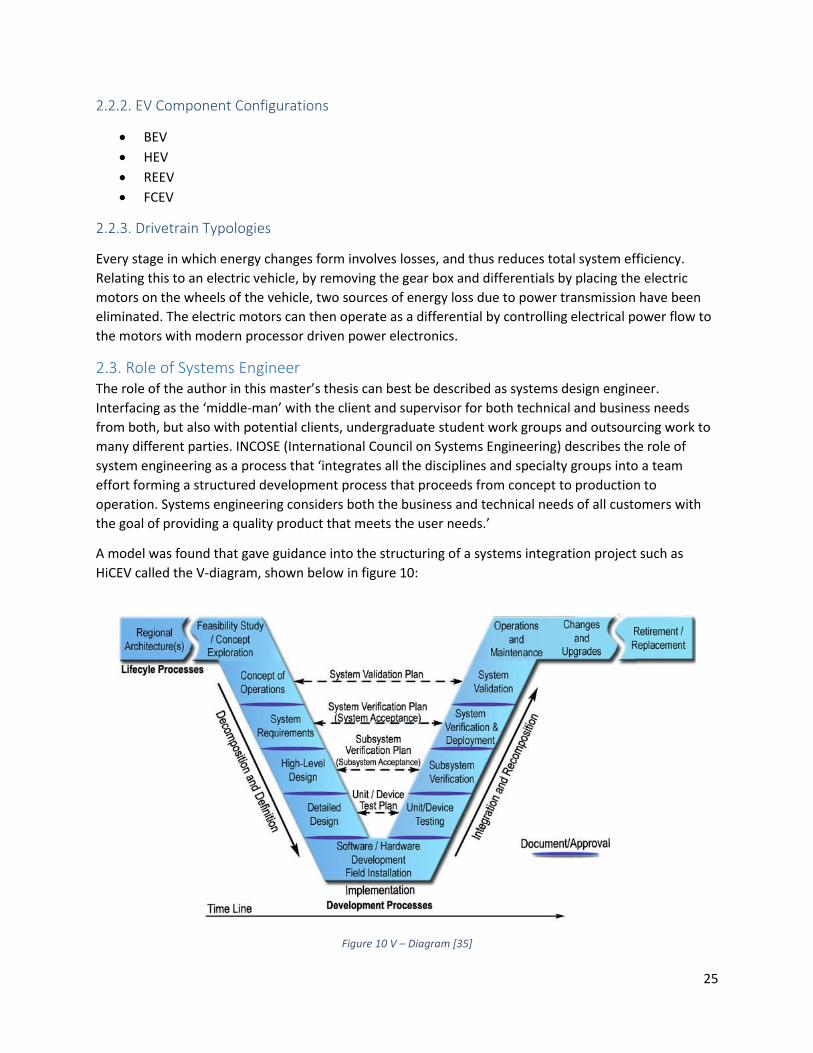
A model was found that gave guidance into the structuring of a systems integration project such as
HiCEV called the V-diagram, shown below in figure 10:
Figure 10 V – Diagram [35]
26
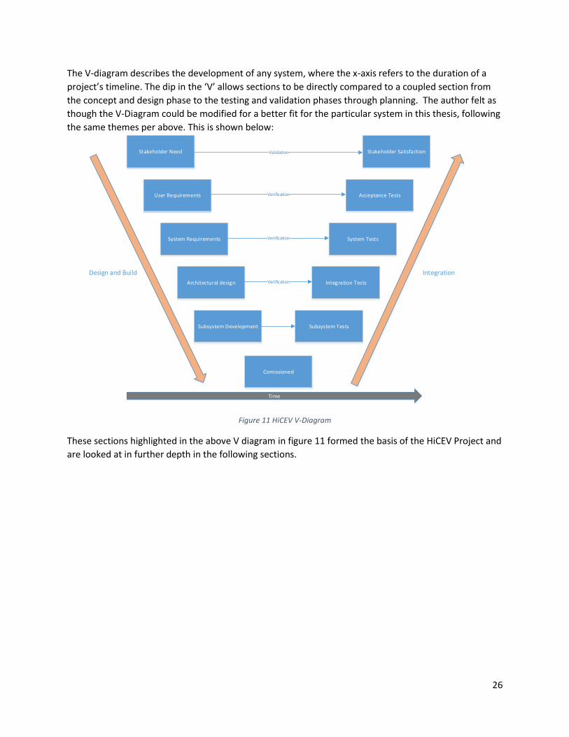
The V-diagram describes the development of any system, where the x-axis refers to the duration of a
project’s timeline. The dip in the ‘V’ allows sections to be directly compared to a coupled section from
the concept and design phase to the testing and validation phases through planning. The author felt as
though the V-Diagram could be modified for a better fit for the particular system in this thesis, following
the same themes per above. This is shown below:
User Requirements
System Requirements
Architectural design
Subsystem Development
Stakeholder Need
Comissioned
Subsystem Tests
Integration Tests
Acceptance Tests
System Tests
Stakeholder Satisfaction
Time
Stakeholder Need
User Requirements Verification
Verification
Verification
Validation
Design and Build Integration
Figure 11 HiCEV V-Diagram
These sections highlighted in the above V diagram in figure 11 formed the basis of the HiCEV Project and
are looked at in further depth in the following sections.

27
3.0 Prototype Specification Design The majority of work conducted in this project was in the areas of ‘Component Selection’ and in
‘Systems Integration’. Testing the vehicle would ideally have the equivalent time allocated as the other
two areas, but due to the nature of the project and time constraints only a few of the many vehicle
aspects were able to be tested and evaluated.
3.1. Stakeholder Requirements The HiCEV project began in 2013 as a collaboration between the Department of Electrical and Computer
Engineering and Glenthorne Station, a high country station in central Canterbury, South Island of New
Zealand situated on the northern side of Lake Coleridge. The client approached the university identifying
their need of a vehicle that would serve as a prototype electric vehicle for farming applications, with the
potential to convert further vehicles in the fleet in the future.
There was a list of initial core requirements for the end product as specified by the client as follows:
Must be capable of farm work
Must be usable by any farmer
Must be fully sealed
Must be capable of regenerative braking
Must be certifiable
These were the base requirements of the project to give an overarching reference when specific
engineering design solutions were being implemented.
3.1.1. Costings Pricing has been omitted from the report. This being due to the fact that HiCEV is a prototype vehicle by
nature thus is generally subject to a great amount of variability as the project progresses.
3.2. User Requirements The following sections detail in depth the requirements laid out by both the client and farmers that will
be using the vehicle.
3.2.1. Client and Intended use The end user group was determined to be both the owner of the farming station and also the farmers.
The three main functions of the vehicle are:
1. Station ‘errand’ vehicle
The station is 25,233.00 hectares in area, and is comprised of two former stations with a twenty
minute drive separating the two. Both stations have their primary use, the lower used for reception,
lodging, vehicle yard and mechanics workshop – the upper used for lodging and managerial
purposes.
2. Station working vehicle
Daily tasks include; carrying fence piles, moving cattle, or a dog-carrying truck for high country
musterers. These are examples of light duty, but the vehicle must also be able to tow loads of

28
fertilizer and possibly other vehicles if required.
3. Prototype show vehicle for events
The client desires the vehicle to be a platform vehicle to show industry that electric vehicles are able
to perform in rough environments. New Zealand has the potential to be a leader in the field of
agricultural EV’s as NZ farmers have proven to be open to using innovative technology enhance
farming practices.
3.2.2. Donor Vehicle A 70 Series Land Cruiser was the donor vehicle in this project shown in figure 11 This vehicle was not
being used extensively in the way of farm work, and was being used as more of a farm run around. It
was in an overall good working condition when the conversion process got underway. Aside from this, it
was the vehicle that the client requested. Toyota Land Cruisers are known as robust ‘workhorses’ in the
NZ farming community. This is important as farmers are familiar with these vehicles thus making the
comparison between the EV and ICE drivetrains easy to distinguish.
Originally an 80 Series SUV Land Cruiser frame was intended for conversion, but this was revised and
changed as having a deck on the vehicle enabled features that are unique, eye-catching and practical. By
being able to detach the deck, much of the planning for component locations could take place with
ease, and later on in the project, accessing these vital components easily was a necessity that would
have been impractical to implement in an SUV.
3.2.3. Off-Road Operation Specific requirements are associated with off-road vehicle operation. The following factors separate
HiCEV from urban EV commuters such as the Nissan Leaf:
Un-sealed road operation (high vibration exposure)
Effective function at low speeds
Operate in rough terrain (and climatic extremes)
Figure 12 HiCEV Donor Vehicle
29
High power High torque
Off-Road vehicles are generally associated with mining, construction, forestry, military and agriculture.
HiCEV is a hybrid of both on-road and off-road effective vehicle; the expectation is that HiCEV will
achieve both requirements at a higher level than the combustion counterpart.
3.2.4. Performance and Drivetrain A change to a vehicles drivetrain is generally the result of a desire for an increase in performance.
Although not the core driving force for the conversion, sufficient performance is required for usability
and product image. Although the client did not have specific performance requirements, it was clear the
user would be discontent with an underpowered system. Hence, the performance factor was driven
from the farmer’s perspective. After consulting with spokesmen for the farmers, the following two
requirements were agreed upon:
More Power than the Original ICE
The farmers reasoning for this was twofold; Firstly, after explaining that the vehicle will gain
some weight due largely to the battery pack, increased electrical power compared to the
original ICE drivetrain is required to obtain similar performance in order to be used as a work
vehicle. Secondly, the farmer that corresponded most with the author was also a mechanic and
quite rightly stated that public interest will increase if it has noticeable performance
improvement. This is in the interest of the client too as the vehicle is to be used as a show piece.
To calculate power requirements, a straight power-to-mass ratio was used to obtain a target
threshold electrical power: 𝑃𝑖𝑐𝑒
𝑀𝑖𝑐𝑒=
𝑃𝑒𝑙𝑒𝑐
𝑀𝑒𝑙𝑒𝑐
Where Pice = 96kW and Mice = 2010kg for the combustion drivetrain. A vehicle mass increase of
~200-300kg is regularly observed in conversions using lithium chemistry battery packs. Pelec can
thus be estimated as:
𝑃𝑒𝑙𝑒𝑐 =96𝑘𝑊
2000𝑘𝑔. 2400𝑘𝑔 = 115 kW
Using the upper end of vehicle conversion weight (300kg) to be conservative, an electrical
power minimum of 115kW was calculated to give similar performance as the original vehicle.
Regenerative Braking is Required
Although less common amongst most electric car conversions due to associated costs,
regenerative braking was set out as a requirement by the farmers. The reason for this is twofold;
Firstly, after explaining the vehicle would likely have a run time (at full power) of approximately
one hour, the farmers wanted the system to employ ways to extend this. The concept of
regenerative braking is simplistic – instead of dissipating energy as heat in traditional friction
brakes, the linear kinetic energy of the moving vehicle (momentum) is converted to electric
energy through rotational couplings to the motor (wheels, differentials, gears and shafts) where
the motor operation shifts to the generating quadrant, providing a retarding torque to slow the
vehicle. The energy cycle ‘round-trip’ (from battery to motor and back to battery) efficiency is
important to determining the percentage of recaptured energy. AC motors and controllers are
able to run in the 90-95% energy efficiency range [36], but there are other losses in the cycle
such as the resistance of cabling and internal impedance of batteries. Below is a simple model

30
that was used to determine, without datasheets, the kinetic energy conversion through
assigning component efficiencies from motor to battery:
𝑒𝑏−𝑚 = 𝑒𝑏 . 𝑒ℎ𝑣𝑟,𝑡𝑜𝑡. 𝑒𝑖. 𝑒ℎ𝑣𝑟,𝑡𝑜𝑡 . 𝑒𝑚
Where em-b is total efficiency from motor to batteries. To make the calculations simpler, the
cable and battery efficiencies were set to 98%. Thus:
𝑒𝑏−𝑚 = 0.98 . 0.95 . 0.97 . 0.98 . 0.95 = 85%
The mechanical rolling efficiency of the vehicle (affected by components producing heat when
the vehicle moves; bearings, CV joints, differentials, gears, wheels) is estimated to be emech =
70%. For electrical round-trip from batteries, eb-m is squared (losses on both power transmission
to motor, and on returning from motor, eb-m =em-b) back to and is multiplied by the mechanical
efficiency which is always present:
𝑒𝑡𝑜𝑡 = 𝑒𝑚−𝑏2 . 𝑒𝑚𝑒𝑐ℎ = 0.85 ∗ 0.85 ∗ 0.70 = 51%
Thus giving a potential maximum of 51% of total transmitted energy (𝑒𝑡𝑜𝑡) recapture. However,
in practice, this number tends to be more in the region of 20% energy recapture [37]. Although
this number seems low, it effectively adds approximately an additional 12 minutes to the drive
time for a one hour cycle (depending on average proportion of time and magnitude of braking in
that hour).
3.2.4.1. Typology
The series electric drivetrain typology was selected from possible configurations shown in figure 13. This
involves one electric motor which takes the place of the original ICE. In this configuration, the gearbox
can either be retained or removed where a directly coupled single fixed-gear ratio is implemented.
Fixed-gearing couples the electric motor directly to a shaft that is fed to the differential, reducing weight
and mechanical complexity by removing flywheel, clutch and gearbox assembly. The short-comings
associated with fixed gear arises especially for low-speed, high-torque applications where the ability to
use 1st gear in combination of the transfer box ratios is of particular benefit.
Flywheel and clutchGear box
Transfer Case
DiffDiff
Motor
Figure 13 Series BEV Typology
As low-speed off-road applications has been defined as one of the requirements; retaining the gear-box
allows for high-ratio gearing (X>>1) for high torque low speed applications and four wheel drive (4WD)
which is difficult to implement without a gearbox. The major short comings of this arrangement include
both the mechanical coupling and electrical implementation on terms of gear sensing for vehicle speed
equations and sensing clutch, both of which are explored in further detail in sections.
31
3.3. System Requirements The prior qualitative analysis highlights the client and user needs, further mathematical definition is
required to give a quantitative analysis. This is achieved through analyzing the vehicle through equations
of motion and modeling electrical and mechanical characteristics, a better understanding of vehicle
performance can be realized before purchasing and implementing a system.
3.3.1. Vehicle Performance Vehicle performance can be modelled by using the kinematic equations of motion for a vehicle. For light
urban vehicles (<2000kg), performance benchmarks. Vehicles which are tested through modeling can
have results compared to these benchmarks to give an indication of relative performance. Commonly
used urban vehicle benchmarks are listed below:
0-97 km/hr: < 12 seconds
64-97 km/hr: < 5.3 seconds
0-140 km/hr: < 23.4 Seconds
These are defined by US Partnership for a New Generation of Vehicle’s (PNGV). Although these
benchmarks do not carry equivalent importance in the case of HiCEV, which will be spending majority of
running time in a low speed off road environment, it will still be on the road at times and as such the
benchmarks are worth evaluating.
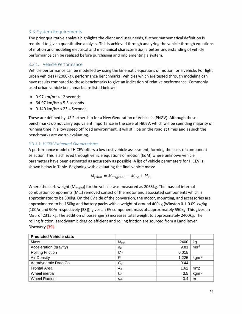
3.3.1.1. HiCEV Estimated Characteristics
A performance model of HiCEV offers a low cost vehicle assessment, forming the basis of component
selection. This is achieved through vehicle equations of motion (EoM) where unknown vehicle
parameters have been estimated as accurately as possible. A list of vehicle parameters for HiCEV is
shown below in Table. Beginning with evaluating the final vehicle mass:
𝑀𝑓𝑖𝑛𝑎𝑙 = 𝑀𝑜𝑟𝑖𝑔𝑖𝑛𝑎𝑙 − 𝑀𝑖𝑐𝑒 + 𝑀𝑒𝑣
Where the curb weight (Moriginal) for the vehicle was measured as 2065kg. The mass of internal
combustion components (Mice) removed consist of the motor and associated components which is
approximated to be 300kg. On the EV side of the conversion, the motor, mounting, and accessories are
approximated to be 150kg and battery packs with a weight of around 400kg (Winston 0.1-0.09 kw/kg
(100Ar and 90Ar respectively [38])) gives an EV component mass of approximately 550kg. This gives an
Mfinal of 2315 kg. The addition of passenger(s) increases total weight to approximately 2400kg. The
rolling friction, aerodynamic drag co efficient and rolling friction are sourced from a Land Rover
Discovery [39].
Predicted Vehicle stats
Mass Mveh 2400 kg
Acceleration (gravity) αg 9.81 ms-2
Rolling Friction Crf 0.015
Air Density P 1.225 kgm-3
Aerodynamic Drag Co Cd 0.44
Frontal Area Afr 1.62 m^2
Wheel inertia Iwh 3.5 kgm-2
Wheel Radius rwh 0.4 m

32
From the original estimate of over 115kW, more vehicle parameters can be refined and base
performance characteristics can be defined. Listed above in Table are the predicted vehicle statistics in
which to calculate the vehicle forces for the HiCEV vehicle model. To determine the vehicle performance
characteristics, firstly Frl (forces due to road loading) must be determined. Frl is the sum forces of rolling
resistance, tractive effort, road grade and aerodynamics. Rolling resistance force is defined below:
𝐹𝑟𝑟 = 0.015 ∗ 2400 ∗ 9.81 ∗ cos (𝛷𝜋
180) = 353.16 ∗ cos (
𝛷𝜋
180) 𝑁
Since vehicle velocity is greater than zero. Aerodynamic drag force at 90km/hr is given as:
𝐹𝑎𝑑 = 0.5 ∗ 1.225 ∗ 0.44 ∗ 1.62 ∗ 252 = 272.90 𝑁
And force due to road grade is:
𝐹𝑟𝑔 = −2400 ∗ 9.81 ∗ sin (𝛷𝜋
180) = −23544 ∗ sin (
𝛷𝜋
180) 𝑁
Where tractive effort force is defined as Fte = Frg + Facc and Tractive force from the motor is calculated
as
𝐹𝑡𝑒 = 𝑇𝑎𝑥𝑙𝑒
𝑟𝑤ℎ𝑒𝑒𝑙=
1768.6
0.37 = 4780 𝑁
Then rearranging eqn above to give acceleration at zero road angle, Φ = 0 from standstill (Fad = 0):
𝑎𝑣𝑒ℎ =4780 − 353.16
2400 = 2.0𝑚𝑠2
Thus, it can be found for a drivetrain of 320 Nm that the acceleration time to get to 100 km/hr
(27.78m/s) is roughly 14 seconds. The energy required to accelerate from 0 – 97 km/hr (27m/s or
60mph) is:
𝐸𝑎𝑐𝑐 =1
2𝑚𝑣𝑒ℎ . 𝑣𝑣𝑒ℎ
2 = 2400 .729
2= 880𝑘𝐽
For an acceleration time of 14 seconds for 0-97 km/hr, the average power required is:
𝑃𝑎𝑣 =𝐸𝑎𝑐𝑐
𝑡=
874800
14~62𝑘𝑊
Headwind vwind 0 m/s
3rd Gear
Torque (engine) Tice 122 Nm
Gear Ratio transmission GR trans 1.49
Gear Ratio Differential GR diff 4.11
Gear Ratio Transfer Case GR tcase 1
GR tot 10.1106
Efficiency transmission e trans 0.95 %
Efficiency differential e diff 0.95 %
Efficiency tcase e tcase 0.95 %

33
And a peak power of:
𝑃𝑚𝑎𝑥 = 𝐹𝑡𝑒 ∗ 𝑉 = 4780 ∗ 27 = 129𝑘𝑊
Where this peak power forms the basis of the motor performance requirement.
3.3.1.2. Regenerative Braking and Range Extension
Current electric vehicles, conversions in particular, do not have the range to compete with their ICE
counterparts in a market sense. As such, methods of extending maximum range capabilities are crucial
in making electric vehicles a competitive solution. Two current ways of extending range aside from
increasing effective battery capacity are regenerative braking and hybridization ICE modules to charge
batteries whilst in operation. These are discussed below.
Regenerative braking converts the vehicles kinetic energy to electrical energy which is fed back to the
battery bank. This helps recover some of the energy lost due to friction (road, mechanical, air) and
acceleration, increasing overall system efficiency. Without taking losses into account, the kinetic energy
and thus the amount of energy recapture of a vehicle moving at 97km/hr is given as:
𝐸𝑘𝑖𝑛,𝑣𝑒ℎ =1
2. 𝑚. 𝑣2 = 0.5 ∗ 2400 ∗ 27 = 874800𝐽 = 0.24 𝑘𝑊ℎ
Which is the same amount as above used for calculating the amount of energy to accelerate to 97km/hr.
Assuming the vehicle has an average speed during deceleration of 27/2 = 13.5m/s, correlating to an
average drag force of 130 N and the rolling resistance is 350N at zero road angle, the energy losses due
to these retarding forces can be calculated as:
𝐹 ∗ 𝑥 =1
2∗ 𝑚 ∗ 𝑎2 ∗ 𝑡2 = 𝐸𝑘𝑖𝑛
𝐸𝑘𝑖𝑛 = 430 ∗ 135 = 58050 𝐽 = 0.0161𝑘𝑊ℎ
At a stopping time of 10 seconds. Without taking mechanical losses into account, (difficult to guess
without a roll down test) the energy that can potentially be recovered from acceleration is 0.24 - 0.016 =
0.23 kWh. This result may, however, be misleading into the reader thinking that ~90% of energy may be
recovered from general commuting, but this however only takes into account the 10 seconds of change
in velocity, and not the time spent overcoming frictional forces at a constant velocity such as for a
motorway drive cycle (no decelerating). For the motorway drive cycle, range extension can only be
achieved by an additional energy source to the batteries – a generator.
Implementing a 3kW petrol generator can act as a range extender element by supplementing energy to
the batteries continuously with the effect of giving a higher effective battery capacity. For an effective
battery capacity of 30kWh, this can be characterized by:
𝐸 𝑒𝑏 =𝐸𝑏
𝐸𝑏−(𝑃𝑔𝑒𝑛 ∗ 𝑡𝑔𝑒𝑛,𝑟𝑢𝑛)
And thus:
𝑡𝑣𝑒ℎ,𝑟𝑢𝑛 = 𝐸𝑏
𝑃𝑏,𝑖𝑛𝑠𝑡 − 𝑃𝑔𝑒𝑛

34
Where:
𝑃𝑚,𝑖𝑛𝑠𝑡 𝑎𝑣 = 𝑃𝑏,𝑖𝑛𝑠𝑡 − 𝑃𝑔𝑒𝑛
Where tgen,run and tveh,run denote the operation runtime of the generator and the vehicle motor
respectively. Combining both range extension and regen braking gives the total effective battery
capacity
𝐸𝑡𝑜𝑡,𝑒𝑏 = 𝐸𝑔𝑒𝑛,𝑒𝑏 + 0.2 ∗ 𝐸𝑒𝑏
Where the regenerative energy is 20% of the effective battery capacity (0.2 ∗ 𝐸𝑒𝑏). This results in a total
effective battery capacity (𝐸𝑡𝑜𝑡,𝑒𝑏) of approximately 39kWh, an increase in 9kWh from an hour’s
operation under the above conditions. From the derivations above, the significant impact that the
combination of a range extender and regenerative braking has on effective battery capacity and thus
run-time.
3.4. Component Sourcing The decision of purchasing main modules consists of locating suitable technologies and employing a
weighting system to choose the best solution for the application. A focus is maintained on the main
components for the vehicle, as the subsystems were evaluated by undergraduate student groups
working on the vehicle.
3.4.1. Motor and Inverter combination A system of reliance is considered to evaluate an appropriate a drivetrain solution. This is shown in
figure [14] below, where the system initiates from user requirements which influences specific
components. The vehicle performance analysis above provides a base approximate sizing of the motor
and inverter combination – these two components are one of the major design decisions.

35
Motor
-Type-Power
-Voltage-Current
Inverter-Availability
-Matches Motor Characteristics
Battery Pack-Inverter DC Bus
-Space restrictions-Discrete AH increments
available-Chemistry
Charger-Battery pack DC voltage
-AC current draw- Programmability-Communication
BMS-Number of cells in pack
-Communication-Charger compatibility
ECU-Able to communicate
effectively to all modules
-User Requirements-Vehicle assessment
-Space
Figure 14 Product sourcing flow diagram

36
3.4.1.1. Motor Selection
A list of motors that would meet the user requirements is listed in table 1.
1Passive Air cooled
Where further weighting factors are defined below in order of importance to HiCEV:
1. Motor maximum power
2. Continuous power
3. Availability
4. Compatibility with inverter systems
5. Regenerative braking compatible
6. Environmental Sealing
7. DC Bus voltage
8. Weight
9. Cost
The motor power requirements have been highlighted in above sections.
Availability is the ability to locate, purchase and ship component.
Compatibility with available inverter systems is an important aspect of integration and is defined
by the matching of both HV electrical characteristics and LV sensor integration. HV power
integration is not only characterized by magnitude of voltage and currents, but the waveform
outputs.
Regenerative braking and environmental sealing ensuring it will be suited to the operation
environment.
HVDC voltage - A higher bus voltage helps with system efficiency – as seen by the equations
below:
𝑉𝑖𝑛𝑣𝑒𝑟𝑡𝑒𝑟 = 𝑉𝑏𝑎𝑡𝑡,𝑡𝑜𝑡𝑎𝑙 − 𝑉𝑠𝑎𝑔
Where:
𝑉𝑠𝑎𝑔 = 𝐼𝑑𝑟𝑎𝑤 ∗ (𝑅𝑏𝑎𝑡𝑡,𝑖𝑛𝑡𝑒𝑟𝑛𝑎𝑙 + 𝑅𝐵𝑎𝑡𝑡,𝑐𝑜𝑛𝑛𝑒𝑐𝑡𝑜𝑟𝑠 + 𝑅𝑐𝑎𝑏𝑙𝑖𝑛𝑔)
And:
𝑃𝑖𝑛𝑣𝑒𝑟𝑡𝑒𝑟 = 𝑃𝑏𝑎𝑡𝑡,𝑡𝑜𝑡𝑎𝑙 − 𝑃𝑙𝑜𝑠𝑠𝑒𝑠,𝑡𝑟𝑎𝑛𝑠𝑚𝑖𝑠𝑠𝑖𝑜𝑛
Motor Vendor
Type Typology Power kWpeak
Power kWcont
DC bus Voltage (Vdc,max)
DC Current (Adc,max)
Regen
Sealed Availability
Netgain HV11 DC series 200 - 288 1000 No No Easy
HPEV 2 x AC75 AC 125 181 144 538 Yes - Easy
Yasa YASA-400 PMAC 165 - 700 - Yes Yes Low
Remy HVH250-115P
PMAC 300 - 700 600 Yes IP67 Medium
UQM PP100 PMAC 135 - 425 400 Yes Yes Medium
Siemens 1PV5135 Induction 100 - 300 400 Yes IP67 Medium
Table 1 Motor Selection

37
Where:
𝑃𝑙𝑜𝑠𝑠𝑒𝑠,𝑡𝑟𝑎𝑛𝑠𝑚𝑖𝑠𝑠𝑖𝑜𝑛 = 𝐼𝑑𝑟𝑎𝑤2 ∗ (𝑅𝑏𝑎𝑡𝑡,𝑖𝑛𝑡𝑒𝑟𝑛𝑎𝑙 + 𝑅𝐵𝑎𝑡𝑡,𝑐𝑜𝑛𝑛𝑒𝑐𝑡𝑜𝑟𝑠 + 𝑅𝑐𝑎𝑏𝑙𝑖𝑛𝑔)
Thus, for a higher current draw, compensation in battery voltage is required to account for the voltage
sag associated with the resistances. To illustrate this two 150kW systems, both with 50mΩ total
resistance (battery IR (internal resistance), interconnects and cabling) at 25oC are compared: First
system is 1000Adc, the other 50Adc max current draw. For 150kW of power at the inverter input side, the
first system has a power loss of 50kW during transmission (75% efficient) compared with 12.5kW loss
from the 500Adc system (92% efficient). Therefore the first system requires a bus voltage of 200Vdc
compared with 325Vdc required for the latter system. The voltage drop through transmission from
battery is linear and can be used to prove the calculated voltages above: first system has a sag of 50Vdc,
the second being just 25Vdc (bringing the voltage at the inverter end to 150Vdc and 300Vdc respectively).
The last motor weighting factors were weight and cost. Most electric motors in the power range
required are 60-100kg – a 40kg weight range which makes negligible difference in total vehicle weight.
From the table below three motor solutions that were chosen to investigate further were the UQM,
Remy and the Siemens. Factors were multiplied as a ‘0’ indicated a missing aspect that was required in
specifications.
Power
Availability
Regenerative
DC
Bus voltage
Ease of
implementing Total Score
Netgain 5 5 0 3 5 0 HPEV 3 5 4 1 2 120 Yasa 4 0 5 5 3 0 Remy 5 3 5 5 5 1875 UQM 3 3 5 4 5 900 Siemens 3 3 4 4 3 432
3.4.1.2. Inverter Selection
Similar to the motor selection, performance and availability are the primary factors for inverter
selection. Manufacturers design inverters to specific motors, where the motor must first be
characterized (flux, inductance, cogging torque and back-EMF). Several inverter manufacturers that
were approached for the project provided this characterizing service, but time constraints associated
with the logistics (shipping a motor from USA to AUS then back to NZ in one case) made this option
impractical.

38
Voltage Current Max Power
Min Operating Max voltage Input Motor Peak Cont. Peak
V V V Adc Arms kW kW Efficiency (%)
Azure DMOC 645 120 400 450 507 414 118 53 97
UQM PP 135 250 425 425 288 235 135 80 95
Rinehart 150DX 50 360 400 551 450 150 150 97
Tritium Wavesculptor200 0 450 450 367 300 165 75 97
Scott Scott 200 200 425 450 600 490 200 55 -
Able to interface
with VCU?
CANbus
Operating Temp.
Rotor Position Sensor
Motor Typology
Supported
Integrated Pre-
charge 2.0A 2.0B Sealed Cooling Min Max Mass
Y/N 11bit 29bit IP Glycol/Water oC oC Kg - - -
Y Y - 54 G/W -40 55 14.7 Encoder BLDC/ PMAC
N
- Y - 67 G/W - 65 27.7 - BLDC -
Y Y Y 6K9K G/W -40 80 10.7 Resolver, Encoder
PMAC/ BLDC/
Induction N
N Y - 65 G/W - - 8.5 Resolver, Encoder,
Hall
BLDC/ Induction
N
N Y - - G/W - - 14 Hall,
Optical BLDC/
Induction Y
Table 2 Inverter Selection
The five choices for inverters are shown above. Table 2 has been broken into two as to fit it in, but is
color coded in the row direction for each inverter. The potential motor and inverter combinations (at
the time of sourcing) as shown below in figure 15:
Remy HVH 250 UQM PP Motor Siemens 1PV5135
Rinehart 150DX WaveSculptor 200 UQM PP Inverter Scott Drive Azure DMOC
Figure 15 Motor Inverter Compatibility

39
Aside from power requirements, low voltage integration between motor and inverter is required to be
considered. Motors use typically encoders, hall-effect or resolver position sensors to output rotor
position information to the inverter, where waveform shape and frequency varies significantly with
sensor technology. Remy has designed their motors with a resolver position sensor, whereas the
Siemens motor uses an encoder. Without any changes to the DSP, this limits the possible inverters that
can be used for each motor. Thermal sensors technology also varies between motors and is also a
consideration in system integration.
The Remy and Rinehart combination of motor and inverter combination was selected from the above.
Although the Scott Drive can provide higher current (600 Arms vs 450 Arms) than that of the Rinehart, it is
not set up to interface with a resolver position sensor. The Remy was selected over the Siemens motor
as the Siemens would not come with warranty, and was significantly lower power than the Remy
(110kW vs 150kW). Although the UQM system was designed as a set combination, thus indicating
reduced systems integration time, the Remy provides more power along with the potential to be
coupled with a higher power inverter in the future.
The last aspect that made the Remy + Rinehart combination appealing was that the availability of these
units, and essential downstream components (BMS, Charger, VCU) were all supplied by one supplier
that had tested these systems prior which should ensure “seamless” integration.
3.4.2. Remaining Main Components Downstream componentry associate with the main modules may be identified after the main
components have been selected, indicated by figure 14 above. In this particular situation, the main
modules that interfaced well with the motor/controller combination were able to be purchased through
the same company.
3.4.2.1. Battery Pack Sizing
The advent of the Tesla model S is changing the public perceptions on EV ‘range anxiety’ with vehicles
capable of traveling 320km on a charge. Unfortunately, achieving these ranges in a vehicle conversion is
still difficult, as combustion vehicle chassis are not designed with battery holding capacity in mind.
The battery pack voltage is dictated by the maximum operating voltage of the inverter (360Vdc).
Prismatic cells were chosen over pouch cells for three main reasons:
1. Availability
2. Enclosure Building
3. Swelling
At the time of souring, prismatic cells were easily attainable and relatively inexpensive when ordered in
bulk. The enclosure of a prismatic cell is rectangular and brittle, which attributes to ease of
implementation when designing an enclosure. Pouch cells require support from above increasing the
complexity of an enclosure. Pouch cells are also prone to more rigorous swelling due to gaseous build up
than prismatic. Due to manufacturing anomalies, cells will swell at different rates and can lead to
rupture or break electronic displays if used to monitor the cells [40].

40
Knowing the inverter input voltage allows the specifics of the battery pack to be determined. The factors
for sizing the battery pack are listed below in order of importance:
1. Volume (real estate).
2. Availability
3. Performance Characteristics
4. Ease of implementing
5. Repeatability
As Lithium batteries can be stacked in any orientation volume is the main concern when assessing the
vehicle for available battery locations. Availability and Performance were weighted this way, as there is
no choice between an attainable and lower performance product and a higher performance but
unattainable product. Availability also includes correspondance, shipping and support.
The battery performance indicators of the narrowed down potential batteries are shown below. All the
batteries are lithium chemistry with exception to the bottom two batterys (Trojan and Exide) that are
100Ah and 50Ah lead acid deep cycle respectively. It is quite clear that the performance of equivalent
lead acid is far inferior, the author had no intention of using lead acid but included them in the table as a
point of reference [41].
From here, the best performance battery looks to be the A123 M20, but the fact that it is a 20Ahr,
means that to get into the 100Ahr region, parrallel connections are required in the order of 4-6 strings (a
string being the number of batteries connected in series to obtain the required pack voltage). This has
the effect of increasing both construction complexity in how to fit batteries in an enclosure it also
increases the wiring complexity and chance of battery system failure by an order of magnitude.
This is where ‘Ease of implementing’ also becomes a factor in the component selection tradeoff – while
still getting the required performance the vehicle requires, the larger capacity and volume cells can be
more easily compiled into a pack and monitored by a BMS. For higher performance applications, the
M20 battery may be the better selection, but to get a prototype implemented with desired
performance, the large prismatic cells in the region of 100AH (to avoid complexity of parallel strings)
are the better solution.

41
Winston batteries were easily accessable at the time of purchase, as it is the EV conversion battery of
choice for the majority of vehicle conversions.
The highest input operating bus voltage for the inverter is the ceiling limit for the battery pack, unless an
expensive and impractical DCDC converter is utilised. Thus, 360V / 3.3V = 109 Cells in series at a
maximum charge voltage of 3.3 V per cell. The graph below shows manufacturers data for discharge
under ‘normal’ temperature:
The inverter has a maximum current draw of 450Adc, therefore the batteries must be capable of
sustaining this output for at least 1 minute. The statistics are shown below:
Manufacturer Model USD/Wh
Gravimetric Energy Density (Wh/kg)
Volumetric Energy Density (Wh/L)
Max Power
Density by
Weight (W/kg)
Burst Power
Density by
Volume (W/L)
Weight of 30 kWhr Pack
Winston LYP90AHA $0.38 96.00 151.45 288.00 3029.01 312.50
LYP100AHA $0.31 91.43 132.27 274.29 2645.32 328.13
Sinopoly LFP90AHA $0.36 92.90 150.11 278.71 750.53 322.92
LFP100AHA $0.36 103.23 166.79 309.68 833.93 290.63
CALB SE60AHA $0.41 76.80 124.62 0.00 1246.19 390.63
SE100AHA $0.41 100.00 154.29 0.00 1234.30 300.00
GBS GBS-
LFMP100AH $0.48 100.00 156.29 300.00 1562.88 300.00
A123 M20 $0.29 112.68 233.48 563.38 4669.54 266.25
Trojan T-1275+ $0.14 35.68 80.63 35.68 483.76 840.91
Exide ORB34DC-
48 $0.38 32.26 67.39 32.26 1010.83 930.00
Figure 16 LYP Discharge curve at different C ratings [38]

42
Batteries Parameter Units Value Notes
Winston WB-LYP100AHA
Nominal Capactiy (Ah) 100.00
Winston battery datasheet
Operational Voltage (Vcharged) 3.65
Operational Voltage (Vdischarged) 3.30
Max Charge Current, ≤3CA
(A) 300.00
Max Discharge Current, ≤3CA (Constant Current)
(A) 300.00
Max Discharge Current, ≤20CA (Impulse Current)
(A) 2000.00
Standard Charge/Discharge
Current, 0.5CA (A) 50.00
Cycle Life at 80% DOD, ≥Times
(Cycle #) 3000.00
Cycle Life at 70% DOD, ≥Times
(Cycle #) 5000.00
Temperature
Temp Durability Of Case (C) 200.00
Operating Temp (charge) (C) 85 to -45
Operating Temp (discharge)
(C) 85 to -45
Monthly Self-dischartge Rate
(%) 3.00
Weight (kg) 3.00
Hand Calculations HV Power Setup
Operating Voltage (Vdc) 356.40
Motor Voltage (Vrms, l-l) 252.01
Max Motor Current (Arms) 450.00
Op Voltage (under load) (Vdc) 288.90 (internal resistance of HV connectios =
150mΩ)
PF** 0.95 ** Presumed PF
Efficiency (%/100) 0.94
Battery Pack (kW) 130005.00 DC max power from batteries
Motor Power (W) 116094.47
Motor Power (kW) 116.09 At the motor
Range Calculations

43
Hand calculations can only provide limited accuracy. Computer simulation tools help provide an
increased accuracy model of a system while in the early feasibility stages of a project to give more
accurate predictions.
The vehicle simulator ADVISOR is used in industry and research to simulate ICE, Hybrid, Fuel Cell or BEV
drivetrains and their performance for various drive cycles. ADVISOR is a GUI extension of Simulink and
Matlab that models in Matlab code system components such as motors, gearboxes, and battery packs to
emulate the physics of a vehicle. This vehicle can then be analyzed on various recorded driving patterns
called drive cycles. In this way, different vehicle typologies can be tested against the same driving cycle
to compare performance.
Battery Pack
Number of cells (WB-LYP90AHA)
(#) 108.00
Total kWh of pack (kWh) 35.64
Available kWh at 70% DoD
(kWh) 24.95 70% DoD = 5000 Cycle life
Available kWh at 80% DoD
(kWh) 28.51 80% DoD = 3000 Cycle Life
Power gained through range extension
(kWh) 2.50 3kW charger estimated output
New Available Pack Power
(kWh) 27.45 70% DoD
(kWh) 31.01 80% DoD
Factoring Regen
% Regen of total Pack Power
(%) 10.00
Power regained through regen
(kWh) 2.74 70% DoD
(kWh) 3.10 80% DoD
Total Potential Available Pack Power
(kWh) 30.19 (DoD + Regen + Range Extender)
(kWh) 34.11

44
A basic model for HiCEV was created and modelled in Matlab. The figure below depicts the drive cycle
manipulated to emulate possible farm driving. It can be noted that there is a large amount of fluctuation
in vehicle speed (blue) and there is a constant road grade (α) incline of 200 feet (α = 1.5%) over the
duration of 15 minutes (green). This drive cycle was manipulated from the NYCC (New York City Cycle)
and was chosen for its general low speed (<40mph) and frequent stopping and starting – to simulate low
speed off-road use.
Figure 18 NYC Drive Cycle
Figure 17 ADVISOR vehicle simulator

45
As can be seen on the X-axis, this drive cycle is 900 seconds, 15 minutes in duration. Thus to get an hour
of commuting, four of these cycles were used back to back, shown in figure 19:
Figure 19 Multiple Drive Cycles
This simulation shows one hour of stopping and starting on constant incline gradient. The top plot shows
the simulated ideal vehicle performance (driver dependent) in red against the drive cycle plot. The
discrepancies in the two speed traces can be attributed due to acceleration required to reach the peak
speeds quickly– to be expected from a farm truck on a semi urban drive cycle.
The top lower graph in figure 19 shows a linear change in state of charge (SOC) of 35%, starting from
maximum capacity over the 1 hour duration using the selected drivetrain and using the vehicle
parameters from the EoM analysis.
3.4.2.2. Remaining main system modules
The main system modules were purchased from New Eagle Control Systems, a Michigan based company
in USA. The motor and controller were a package, along with the auxiliary main modules that have
compatibility for reduced system integration complexity. The main system modules communicate
through CANbus as shown below:
Inverter VCU BMS
ChargerVeeCAN Display
120 Ohm 120 Ohm
CAN Hi
CAN Lo
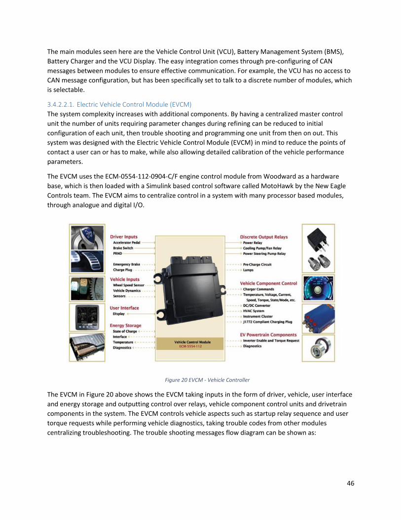
46
The main modules seen here are the Vehicle Control Unit (VCU), Battery Management System (BMS),
Battery Charger and the VCU Display. The easy integration comes through pre-configuring of CAN
messages between modules to ensure effective communication. For example, the VCU has no access to
CAN message configuration, but has been specifically set to talk to a discrete number of modules, which
is selectable.
3.4.2.2.1. Electric Vehicle Control Module (EVCM)
The system complexity increases with additional components. By having a centralized master control
unit the number of units requiring parameter changes during refining can be reduced to initial
configuration of each unit, then trouble shooting and programming one unit from then on out. This
system was designed with the Electric Vehicle Control Module (EVCM) in mind to reduce the points of
contact a user can or has to make, while also allowing detailed calibration of the vehicle performance
parameters.
The EVCM uses the ECM-0554-112-0904-C/F engine control module from Woodward as a hardware
base, which is then loaded with a Simulink based control software called MotoHawk by the New Eagle
Controls team. The EVCM aims to centralize control in a system with many processor based modules,
through analogue and digital I/O.
The EVCM in Figure 20 above shows the EVCM taking inputs in the form of driver, vehicle, user interface
and energy storage and outputting control over relays, vehicle component control units and drivetrain
components in the system. The EVCM controls vehicle aspects such as startup relay sequence and user
torque requests while performing vehicle diagnostics, taking trouble codes from other modules
centralizing troubleshooting. The trouble shooting messages flow diagram can be shown as:
Figure 20 EVCM - Vehicle Controller

47
Charger
Inverter
BMS
VCU
VeeCAN Display
User PC
Trouble Codes User Interface
Where the ‘VeeCAN’ is a small LCD screen with a graphical display, used primarily for the client to refer
to – displaying basic diagnostic data, but mainly basic operating parameters such as coolant temp and
pressure.
3.4.2.2.2. Battery Management System (BMS)
The Battery management system (BMS) that is compatible with the VCU unit is the 108 cell Orion BMS.
The wiring diagram for this unit and the connections the BMS has with the user PC, the charger, current
sensor, thermal systems and the battery pack itself, figure 21.
The battery pack is the most expensive single part of an electric vehicle. The battery pack is made up of
multiple cells, 108 in the case of this vehicle with each cell varying in capacity and voltage slightly (or
sometimes noticeably) from neighboring cells due to unavoidable manufacturing imperfections. With
this in mind, a pack is only as strong as the weakest cell, if a pack of cells is charged at a constant voltage
equal to the multiple of the number of cells by the maximum cell voltage, a range of cell voltages will
evolve at the high end of the charge cycle (last 10% of capacity). The highest of these voltages will be the
weakest cell in the pack, thus resulting in overvoltage and damage to the cell if nothing prevents it from
breaching the maximum voltage threshold. This is where the BMS helps by shunting power from the cell,
Figure 21 Orion BMS Layout [51]
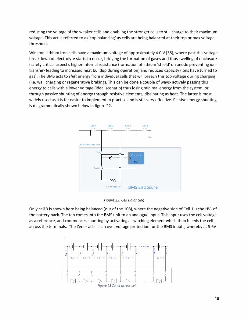
48
reducing the voltage of the weaker cells and enabling the stronger cells to still charge to their maximum
voltage. This act is referred to as ‘top balancing’ as cells are being balanced at their top or max voltage
threshold.
Winston Lithium Iron cells have a maximum voltage of approximately 4.0 V [38], where past this voltage
breakdown of electrolyte starts to occur, bringing the formation of gases and thus swelling of enclosure
(safety critical aspect), higher internal resistance (formation of lithium ‘shield’ on anode preventing ion
transfer- leading to increased heat buildup during operation) and reduced capacity (ions have turned to
gas). The BMS acts to shift energy from individual cells that will breach this top voltage during charging
(i.e. wall charging or regenerative braking). This can be done a couple of ways- actively passing this
energy to cells with a lower voltage (ideal scenario) thus losing minimal energy from the system, or
through passive shunting of energy through resistive elements, dissipating as heat. The latter is most
widely used as it is far easier to implement in practice and is still very effective. Passive energy shunting
is diagrammatically shown below in figure 22.
Processor
Cell #3 BMS wire taps
BMS Enclosure
Fuse
Switch
Shunt Resistor
Cell 1Cell 2Cell 3Cell 4
HV-
IN
OUT
Figure 22: Cell Balancing
Only cell 3 is shown here being balanced (out of the 108), where the negative side of Cell 1 is the HV- of
the battery pack. The tap comes into the BMS unit to an analogue input. This input uses the cell voltage
as a reference, and commences shunting by activating a switching element which then bleeds the cell
across the terminals. The Zener acts as an over voltage protection for the BMS inputs, whereby at 5.6V
Figure 23 Zener across cell

49
the Zener conducts and the internal fuse blows. How the Zeners and fuses are configured with multiple
cells is shown below:
The maximum shunt current for each cell is 200mA and the maximum heat dissipation is approximately
40 W from the BMS unit, thus giving a total of 55 cells (using a 3.5V threshold) that can be balanced
simultaneously. Additionally this shunting current can initiate one of two ways: the cell voltage
threshold (3.5V-3.65V) or difference between max cell voltage and min cell voltage.
The BMS calculates limits based on the thermal profile of the batteries. Internal resistance of a cell, and
thus the output voltage of a cell changes with temperature. To monitor the cell temperature, 3
thermistors are utilized by the BMS to sense the temperature of the cells. Thermal breakdown of the
cell’s electrolyte occurs at around 60o C which forms gas that is vented if internal pressure breaches an
engineered value. Rapid formation of gas can also cause cell rupture, thus for either scenario to be
avoided, the temperature of the cells must be kept below this threshold. Thermistors must be attached
to thermally conductive parts, figure 24, of the battery that are in contact with the cell electrolyte –
even this will not be a perfect indication.
Figure 24 Thermistor Placement
3.4.2.2.3. Battery Charger
The compatibility between the BMS and the charger is important as both over-charging and under-
charging of batteries must not occur, therefore effective communication between BMS and Charger is
essential.

50
The chosen charger for the vehicle was the Eltek 3kW charger in an IP67 sealed rated enclosure. This
charger must be controlled via the CANbus to operate. A diagram of how the BMS and the Charger
integrate is displayed below:
This charger meets the user requirements as follows:
Availability
Meets Environmental Constraints
IP 67 sealed
-40 to 40oC operating range
Compatibility
Both with NZ AC input voltage (230Vac, 50Hz)
3kW Capable, aligns with standard output
BMS CANbus communication
Spans required HVdc range
The Eltek charger parameters below in table 3 meet the specifications required of the charger.
EV Power Charger 360/3000 HE IP67 G2
Input Voltage 85-275 Vac, 50Hz (230Vac nominal)
Input Current 14 Arms
Output Voltage Range 250-420 dc
Output Current 10 Adc
Power Factor 0.99 (@ 50% load or higher)
Charge Control CANbus
Ripple and Noise <250 mVrms
Efficiency 96%(@50% load) - 95%(@100% load)
Operating Temp -40 to 60 oC
Storage Temp -40 to 85 oC
Dimensions 60 x 355 x 167 mm
Weight 4.3 kg Table 3 Eltek Charger Specs
3.5. Main Architectural Design The physical design process regarding placement of components was important to effective system
integration in HiCEV. Careful thought is required in how to use space effectively while maintaining the
performance of the systems left in place (i.e. Brakes, 12V system, lights, steering, and chassis integrity).
Figure 25 Interfacing with Eltek Chargers [52]

51
With this in mind this section aims to detail the process of physical layout of components, from the
general main component layout to the in depth mechanical and electrical connection designs.
3.5.1. Component Layout The vehicle was stripped and measured as shown in figure 26. This allowed measurements to be taken
as to how the systems would interface physically. Deciding where components are going to be placed is
a significant design choice, although with some components, there is not much choice i.e. the motor has
to be in line with the pre-existing driveshaft. At this point it is useful to break down the system
dependencies, i.e. the requirements of successful integration.
After the vehicle was stripped, available space could be measured and a clearer understanding of how
components would interface took place. Spatially, the vehicle can be broken down into three
compartments; the engine bay, the cab and the deck (or rear), as depicted in figure 27:
Engine Bay Cab Deck
Figure 27 Spatial view
Table 4 HiCEV Stripped Figure 26 HiCEV Stripped

52
A bird’s eye approach is useful for seeing how the components will interface on a broad level.
The largest constraints facing the component layout are detailed in the diagram figure 28:
Motor
Pre-Existing drivetrain
Motor Shaft must spigot true to drivetrain
Battery Boxes
Must fit without significant chassis modification
InverterPhysically close (HVac)
BMS1.8m Battery cell wire taps
HV Protection Box
Close proximity (unprotected HVdc cable)
Figure 28 Main Constraints on Component Placement
The components and their downstream dependencies are depicted by the arrow directions. Main spatial
dependencies stem primarily from the pre-existing drivetrain, and secondarily from the motor and the
battery locations. The primary concerns for motor and battery boxes are alignment of the motor shaft
with the driveshaft and supporting enough space for the batteries without cutting away structural
chassis components respectively. Secondary dependencies consist of:
Location of inverter in order to keep EMI (electro-magnetic interference) from HVac reasonably
low
location of HV protection box for adequate isolation and location of BMS so the wiring looms
can reach every cell in the battery pack without requiring lengthening.

53
The choices of where to place the primary spatial concerns are shown superimposed over the vehicle
chassis mechanical drawing shown in figure 29.
The location of the motor was dictated from the transmission input shaft which is shown in the drawing;
central, along the mid-line of the vehicle. The battery boxes require the maximum space allowable
without affecting vehicle performance. The mass distribution and thus the center of gravity (COG),
brakes and suspension is dependent on battery mass placement.
The station mechanic was crucial here in declaring safety distances from driveshaft and suspension. The
boxes were designed to sit above the chassis rail to reduce the chance of impact from underneath. The
rear lateral support that Box 2 interferes was not classified as structural (it provided a place for the
spare wheel to fasten) and therefore was removed.
3.5.2. Electrical Layout The electrical layout was split into three categories: High Voltage Power, Low Voltage Power and
Communications, a flow diagram of component interconnection is shown in figure [30]. High voltage is
defined as anything in excess of 50Vdc, where low voltage power focuses on the 12V vehicle auxiliary bus
and communications is the combination of CANbus and Serial communication. An initial bird’s eye
approach of the electrical layout of the components spatially in the Appendix 7.1.
Box 1
Bo
x 2Motor
Trans
Figure 29 Battery Box placement

54
ICE GeneratorBattery Charger
Battery Bank Energy Source
Power Converter
Motor Wheels
Tools
12V battery Charger
BMS
EVCM
HV Protection
Glycol Cooling
Oil Cooling
Power Steering
Vacuum Brakes
Figure 30 Electrical Power Flow
3.5.3. Mechanical Layout Mechanical layout details the way devices physically connect to the vehicle. The specific connections of
consequence are the motor shaft connection to the drive train and placement of the battery box.
3.5.3.1. Motor to drivetrain
Effective coupling of motor to the drivetrain is crucial for power transmission. The Remy motor has
internal bearings that support the rotor. They are only designed to support the motor mass and
gyroscopic forces on the rotor [42]. Therefore to couple the flywheel to the motor, an adapter shaft with
separate bearings needed to be designed to take the radial and axial loading of the flywheel mass and
the clutch engaging respectively. The basic initial idea behind this is depicted graphically in figure 31.
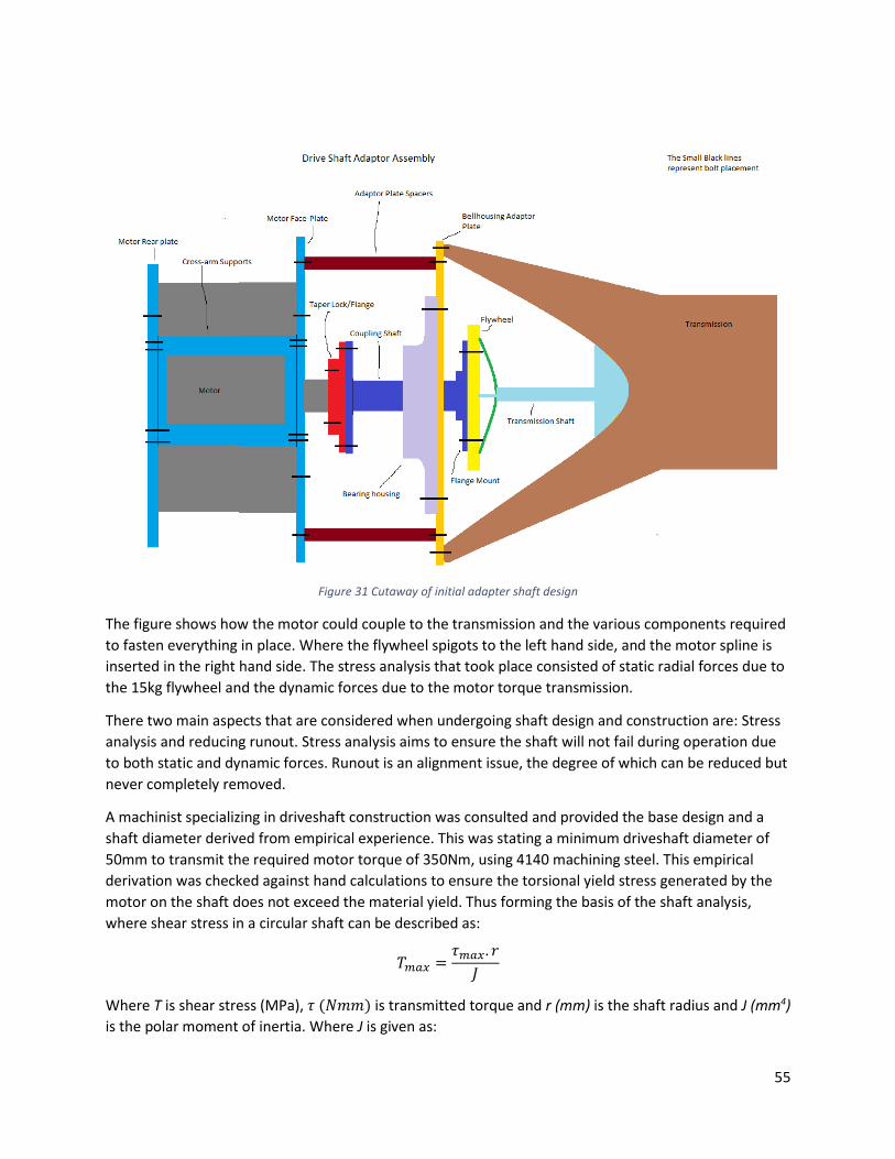
55
The figure shows how the motor could couple to the transmission and the various components required
to fasten everything in place. Where the flywheel spigots to the left hand side, and the motor spline is
inserted in the right hand side. The stress analysis that took place consisted of static radial forces due to
the 15kg flywheel and the dynamic forces due to the motor torque transmission.
There two main aspects that are considered when undergoing shaft design and construction are: Stress
analysis and reducing runout. Stress analysis aims to ensure the shaft will not fail during operation due
to both static and dynamic forces. Runout is an alignment issue, the degree of which can be reduced but
never completely removed.
A machinist specializing in driveshaft construction was consulted and provided the base design and a
shaft diameter derived from empirical experience. This was stating a minimum driveshaft diameter of
50mm to transmit the required motor torque of 350Nm, using 4140 machining steel. This empirical
derivation was checked against hand calculations to ensure the torsional yield stress generated by the
motor on the shaft does not exceed the material yield. Thus forming the basis of the shaft analysis,
where shear stress in a circular shaft can be described as:
𝑇𝑚𝑎𝑥 =𝜏𝑚𝑎𝑥. 𝑟
𝐽
Where T is shear stress (MPa), 𝜏 (𝑁𝑚𝑚) is transmitted torque and r (mm) is the shaft radius and J (mm4)
is the polar moment of inertia. Where J is given as:
Figure 31 Cutaway of initial adapter shaft design

56
𝐽 = 𝜋. 𝐷4
32
Where D is the shaft diameter. Thus Table 5 gives the results:
Parameter Value
D 50 mm
J 613592 mm4
𝜏max 350000 Nmm
R 25 mm
Tmotor torque 14.3MPa Table 5 Shaft Parameters
Thus the motor produces a shear torsional stress of 14.3MPa. The yield strength of 4140 is in the order
of 500MPa (atmospheric conditions), sufficiently high to negate torsional effects.
Radial forces are also considered, where the shaft acts as a cantilever from the motor if unsupported.
Due to the mass of the flywheel, support must be employed on the shaft to eliminate loading the rotor
bearings. Observing figure 32, shifting the point of support or fulcrum from position 1 to 2, the torque is
reduced proportional to the difference in distance.
2 1
Figure 32 Shaft support
This support must be in the form of a bearing, since the shaft will be rotating. Thus the bearing is
required to eliminate the radial loading. A second support bearing is utilized here at the motor end of
the shaft. This ensures the pivoting of the shaft around the flywheel end bearing doesn’t cause vertical
radial loading on the rotor bearings, thus a different design is employed to that of figure 33

57
Runout occurs in every rotating system and increases bearing wear which can have a range of
downstream effects, from impeded performance through to system failure. The motor bearings are the
crucial parts here, as they cannot be easily accessed for maintenance. Runout of a system can be
measured by dial indicator, but due to the inaccessibility of the system, estimates were employed.
Figure 33 Secondary Adaptershaft Design
Figure 34 Shaft runout [53]

58
The final shaft design was designed in CAD. The five main design constraints consisted of; Mechanical
loading on the motor and shaft, the length of the shaft from motor to transmission, correct 24-tooth
spline dimensions for motor connection, bearing placement and flywheel attachment. The final
driveshaft is shown in figure 35 and the associated bearing housing in figure 36.
Figure 35 Final Adapter Shaft

59
3.5.3.2. Battery Boxes
Battery placement impacts vehicle perfomance and systems integration. The battery weight is ideally
situated as low as feasable on the vehicle, this helps with stability by making it more difficult to allow
the vehicle center of gravity outside the vehicle basis of support (wheel base when all four wheels are
on the ground). The 70 Series landcruiser has two chassis rails running the length of the vehicle. These
rails give two major benefits for battery placement:
1. Secure place to fasten to
2. Provide impact protection
3. These chassis rails are shown below wiith the battery box layout superimposed:
Braking is also affected by vehicle mass distribution. By taking weight out of the front when removing
the motor and putting back less than half that with the electric drivetrain, suspension and thus brakes
will be less loaded in the front. To compensate for this, battery weight has been designed to be
distributed over both axles, by having the majority of battery weight in the middle of the vehicle.
Figure 36 Bearing Housing

60
Figure 37 Battery Box location
Main battery box (box 1) placement is shown in the above Figure 37, where approximate clearances for
chassis twist were taken into account to ensure the driveshaft did not impact against the box. From this
sketch of dimensions in figure 38, a CAD drawing was constructed with more specific dimensions
relating to placement orientation of the 108 x 100Ah Winston cells in Appendix 7.2
Box 1
Figure 38 Hand measuring the available space

61
To keep the battery box bottom above the chassis rails, the total height of the battery boxes was found
as 300mm through hand measurements. The battery sits at a height of 218mm, and with interconnects
and HVDC cable also in the box, a total clearance of 19mm was calculated as shown in Table 6 below.
3.1 Subsystem Development This area of vehicle development was largely worked upon by the two final year undergraduate
engineering projects that ran during 2014 and 2015. The undergraduates were assigned individual
accessory modules and guidance by the author. The modules that were developed are listed below:
2014
Jack Stanton:
o Motor Cooling
o HV Cabin Heater
Jonathan Sapson
o Inverter Cooling System
o Electric Power Steering
Matt Barnham
o Dash Instrument Cluster interface
2015
Battery Height Calculations Units Value
Height of Battery Mm 218
Braided Interconnects Mm 15
Bolt Head Height Mm 10
DC Cable thickness Mm 20
Insulation thickness mm 2
Aluminum Thickness mm 6
Double floor mm 10
BMS wiring? -
Top supports mm
Allowed Space mm 300
Total Clearance mm 19
Table 6 Battery box height calculations

62
Bram Humphris
o Charger changeover switching unit
o Inverter Calibration
o Battery Testing
Mitch Graham
o Inverter Commissioning
o HV Safety Box Fabrication
o Battery Testing
Devesh Sanjay
o Charger implementation
o General Wiring
3.1.1 Thermal Systems There are three main thermal management systems on the vehicle associated with EV Components:
Motor cooling, Inverter cooling and the Charger cooling. The BMS also has elements of cooling
associated with it that will discussed later, but it does not require an external thermal management
system.
Project Supervisor
Client
Progress Reporting
Specifications
Technical advisor

63
3.1.2 Motor Cooling Oil cooled HVH motors have oil-cooled stators and rotors. In oil cooled versions of the motor, oil is fed
into the cooling jacket and flows from there over the end turns in the sump. This flow path ensures
additional cooling to both the rotor and stator allowing higher power outputs for longer durations than
would be allowable without the rotor cooling path. Cooling reduces the negative impacts associated
with the motor such as: winding insulation break down, bearing seals degradation and the rotor
magnets do not de-magnetize as they approach the reaching Curie temperature point.
Figure 39 Motor Temperature Limits [42]S
Circulation of cooling fluid is a basic operating mode for the motor, a failsafe that is also built into the
thermal system is current derating. This graph shows the de-rating that occurs to avoid demagnetization
of the stator before reaching the Curie temperature. At 160oC the de-rating starts, and has a linear
decline to 180oC where the inverter limits current to 0, figure 39. The permanent magnets in the HVH
series motors are chosen for their high magnetic flux density and coercivity and are further protected
from demagnetization by the motors’ basic design. Temperature sensors are integrated into Remy
motors, which signal the inverter to reduce current when pre-set thermal limits are approached

64
Figure 40 Motor Coolant pathway [42]
The bearings are also lubricated by the coolant oil. The motor application manual states that a filter is
mandatory oil cooled Remy motors and to use only approved oils to avoid insulation break down and
other negative effects. The cooling requirements are given below:
Fluid: (ATF) Dexron VI
Flow rate: 5-15 L/min
Fill point: op level > 100 mm below shaft center
The application manual gives a basic schematic figure 41 which details pump and heat exchanger
configuration. The motor is configured as a ‘dry sump’ which means that oil is stored externally from the
motor in a reservoir. A more accurate cooling schematic is shown below with components required
figure 42.
Figure 41 Example Cooling schematic [42]
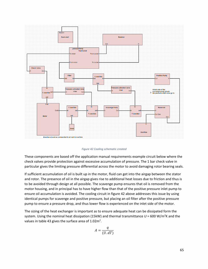
65
Figure 42 Cooling schematic created
These components are based off the application manual requirements example circuit below where the
check valves provide protection against excessive accumulation of pressure. The 1 bar check valve in
particular gives the limiting pressure differential across the motor to avoid damaging rotor bearing seals.
If sufficient accumulation of oil is built up in the motor, fluid can get into the airgap between the stator
and rotor. The presence of oil in the airgap gives rise to additional heat losses due to friction and thus is
to be avoided through design at all possible. The scavenge pump ensures that oil is removed from the
motor housing, and in principal has to have higher flow than that of the positive pressure inlet pump to
ensure oil accumulation is avoided. The cooling circuit in figure 42 above addresses this issue by using
identical pumps for scavenge and positive pressure, but placing an oil filter after the positive pressure
pump to ensure a pressure drop, and thus lower flow is experienced on the inlet side of the motor.
The sizing of the heat exchanger is important as to ensure adequate heat can be dissipated form the
system. Using the nominal heat dissipation (15kW) and thermal transmittance U = 600 W/m2K and the
values in table 43 gives the surface area of 1.02m2.
𝐴 =𝑞
(𝑈. 𝑑𝑇)

66
Parameter Value
Peak Power 130kW
Min Efficiency 78%
Max Heat Dissipation 28.6kW
Assumption, nominal dissipation 15kW
U 600W/m2.K
Oil Temp 70oC
Air Temp 35oC
Area 1.02m2
Figure 43 Cooling sized by Jack
These cooling calculations and sizing’s were completed by Jack Stanton, but were crucial to getting
HiCEV to a moving state.
3.1.3 Inverter Cooling The Rinehart inverter electronics are encased in a CNC aluminum billet, which acts as an excellent
passive heat exchanger in itself. To enable such a small footprint, additional active cooling is also
required. The inverter cooling is a much easier concept than the motor. The glycol/water heat exchanger
cooling requirements are given below in table 7 [43]
The cooling circuit diagram is shown in figure 44. The check valves have not been properly implemented
across the motor or across the inverter, but are vital in avoiding over pressure situations.
Table 7 Inverter Cooling
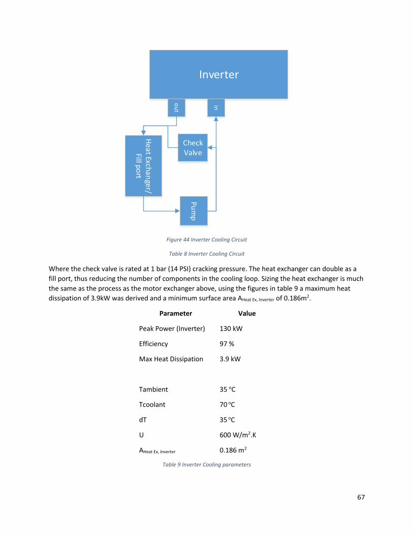
67
Inverter
ou
t
in
He
at Exch
an
ger/
Fill po
rt
Pu
mp
Check Valve
Figure 44 Inverter Cooling Circuit
Table 8 Inverter Cooling Circuit
Where the check valve is rated at 1 bar (14 PSI) cracking pressure. The heat exchanger can double as a
fill port, thus reducing the number of components in the cooling loop. Sizing the heat exchanger is much
the same as the process as the motor exchanger above, using the figures in table 9 a maximum heat
dissipation of 3.9kW was derived and a minimum surface area AHeat Ex, Inverter of 0.186m2.
Parameter Value
Peak Power (Inverter) 130 kW
Efficiency 97 %
Max Heat Dissipation 3.9 kW
Tambient 35 oC
Tcoolant 70 oC
dT 35 oC
U 600 W/m2.K
AHeat Ex, Inverter 0.186 m2
Table 9 Inverter Cooling parameters

68
3.1.4 Charger Cooling Charger Cooling was completed by Devesh, and consists of a passive air cooled heatsink.
3.1.5 Power Steering Power steering was completed by Jono, and implements an electric Holden Astra power steering pump.
The current configuration is such that the 12Vdc bus is pulled low due to current draw at low speed
turning from the power steering pump, which breaches the 9Vmin operating region of the EVCM, so the
vehicle loses power.
3.1.6 Dash Cluster Dash cluster driver board was made by Matt to driver the cluster gauges from CANbus vehicle
information, and still requires work to interface to the CANbus system.
3.1.7 Change Over switching unit The changeover switching unit was developed by Bram and allows the charger to switch between an
onboard generator source implemented as a range extender and the wall socket power. This is a break-
before-make arrangement to avoid sourcing from two places. This circuitry has RCBO to trip if mains
voltage leaks to chassis GND.
4.0 Testing and Commissioning This section was the most time and energy intensive part of the project.
It has been structured so that the details of software used on each module are incorporated into each
module’s section. This is opposed to giving the software components their own section as the author
feels that the focus could be easily diverted away from the data and vehicle performance.
4.1 Main Modules The system of HiCEV are comprised of six main modules: Motor, Inverter, Batteries, BMS, Charger and
EVCM. It is around these components that sub-systems form. Based on the prototyping specifications a
final system was determined in table 10 below.
HiCEV Main Modules Module Type Vendor
Motor Remy HVH250-115-PO New Eagle -Remy Inc
Inverter Rinehart 150DX New Eagle – Rinehart Motion Systems
Batteries 108 x 100Ah Winston Battery Winston Battery
BMS Orion 108 Cell BMS New Eagle – Orion BMS
Charger Eltek 360/3000 IP67 New Eagle – Eltek Valere
EVCM ECM-5554-112-0904-C/F New Eagle – New Eagle/Woodward Table 10 Final main modules
This can be visualized by figure 45 below that shows the main modules centralized and their sub-system
dependencies surrounding them. To simplify the diagram, both the interconnectedness of modules
through the CAN network and the mechanical fastening have been omitted.
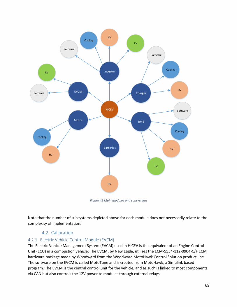
69
EVCM
Inverter
Motor
Batteries
BMS
Charger
HiCEV
Cooling
Cooling
Cooling
Cooling
HV
HV
HV
HV
HV
LV
LV
LV
Software
Software
Software
Software
Figure 45 Main modules and subsystems
Note that the number of subsystems depicted above for each module does not necessarily relate to the
complexity of implementation.
4.2 Calibration
4.2.1 Electric Vehicle Control Module (EVCM) The Electric Vehicle Management System (EVCM) used in HiCEV is the equivalent of an Engine Control
Unit (ECU) in a combustion vehicle. The EVCM, by New Eagle, utilizes the ECM-5554-112-0904-C/F ECM
hardware package made by Woodward from the Woodward MotoHawk Control Solution product line.
The software on the EVCM is called MotoTune and is created from MotoHawk, a Simulink based
program. The EVCM is the central control unit for the vehicle, and as such is linked to most components
via CAN but also controls the 12V power to modules through external relays.

70
How the EVCM oversees the control of modules is shown below in figure 46; where the blue
connections represent 12V power control, green represents CANbus flow, and black represents analog
information.
EVCMInverter
ACC Pedal ADC
Clutch Switch
12V
Brake Switch
12V
Motor
Battery Pack
BMS
CANvu Display
Charger
CANbus
PC Connection
Accessory Power
DCDC Converter
Dash Cluster
CANbus
12V power
Pre-Charge
Figure 46 EVCM Control

71
The motor and battery pack are included here, as the motor feeds the inverter data such as rotor
position from the resolver sensor and temperature which is the used by the EVCM to calculate
important information such as vehicle speed and current derating on torque requests. Similarly, battery
information such as cell voltage, state of charge and temperature are processed by the BMS and utilised
by the EVCM control system to operate the vehicle within safe limits. Also worth noting is that only four
of the six modules that utilise CANbus feed information into the EVCM, whereas five of the six modules
are controlled by the CANbus transmissions from the EVCM. That is, the BMS controls the charger
directly during the charge cycle, but the EVCM can see the charging data.
4.2.1.1. EVCM Hardware, Control and Implementation
The EVCM is supplied by Woodward, then programmed through MotoHawk at New Eagle Control to
perform various tasks in different industries. The EVCM is the electric vehicle controller version based on
this common hardware platform.
ECM-5554-112-0904C/F Hardware
The hardware platform for the EVCM is the Woodward ECM-5554-112-0904C/F engine control module.
From the modules name, it is implementing a Freescale 5554 micro-processor, 112 available pins in
table 11:
PARAMETERS
Microprocessor Freescale MPC5554, 80MHZ
Memory 2MB Flash 64K RAM 32K Cache 32K EEPROM
Calibratable memory 2 x 256K RAM
Operating Voltage 9-16Vdc 24Vdc (Jump start)
4.5Vdc (crank)
Operating Temperature -40 to 105 Deg C
Input Types 33 Analog 4 Oxygen Sensor (Not Required) 3 Speed 2 Knock Sensor (Not Required) 1 Emergency Stop
Output Types 14 Low Side Driver (LSO) 8 Injector 8 Electronic Spark 1 Tachometer 1 Digital Output 1 Main Power Relay Driver 2 H-Bridge Outputs
Communications 3 x CAN 2.0B Channels 1 x RS-485 Channel
Table 11 Woodward Vechicle Contol Specs [44]
The ‘C’ and ‘F’ in the product name denotes Calibratable and Flash versions of the controller
respectively. Flash versions are pre-loaded from supplier with desired engine characteristics but retains

72
base level client-programmability for production applications. The calibratable version allows increased
programming flexibility which includes field calibration and therefore is more suited for prototyping
applications such as HiCEV.
Three sealed ‘pockets’ are built into the EVCM to provide the pinouts to the three Molex connectors A, B
and C which are also color coordinated as black, brown and grey respectively. Figure 48 shows how the
connectors are configured:
Figure 47 EVCM Pinout
Control
The EVCM allows for standard vehicle inputs such as brake and accelerator pedal to implement vehicle
startup and control. Vehicle startup involves moving through a stepwise process to allow safe transition
from a zero power state to operating mode. The steps are listed below in order:
1. EVCM Sense 12V and enable other components power through relay control

73
2. HV Sense
a. Pre-Charge Sequence
b. Close Main Contactor (Make-before-Break logic)
3. Foot Brake Sense – Inverter enable over CANbus
4. Vehicle ON
The key switch 12V ignition circuit has been retained, with modifications to the components engaged at
ACC and IGN 12 Sources. A pre-charge sequence whereby the internal HVDC bus capacitors in the
inverter requires a minimum three RC time constants [43] to charge. This part of the startup sequence is
important as pre-charging prevents high inrush currents to the capacitors
EVCM
ACC Pedal
ADC
Clutch Switch
12V
Brake Switch
12V
PRND Switches
12V
Component Power: Main Power Relay, BMS, Inverter, DCDC Converter
12V
Relay Control: - Pre-Charge (Precharge, Negative and positive
contactors)
- Accessories (Power Steering, Cooling Fan, Cooling pump)
- Charging (Charge Enable)
12V
Table 12 EVCM Control Flow
Torque Requests
HiCEV can either be setup so that the inverter has torque requests sent directly to it, or sent over the
CANbus by a central control unit – the EVCM. The EVCM allows the extreme end of customization in
terms of vehicle torque mapping - based on parameters such as user pedal inputs, vehicle speed,
temperature of modules and battery state of charge.
These EVCM aspects that control the inverter power flow to the motor are shown in Figure 48. The
pedal inputs are all ADC controlled, where the accelerator pedal is an ADC controlled value, based on a

74
dual position sensing (for redundancy) using both a 5V and 2.5V analog input. The brake and clutch
switch are both 12V switch signals (also ADC threshold controlled).
The module parameters such as vehicle speed (which is derived from the motor speed), motor
temperature, inverter temperature, battery state of charge and battery temperature are used to scale
the torque request to avoid component degradation.
EVCM
InverterCANbus
ACC Pedal
ADC
Clutch Switch
12V
Brake Switch
12V
Module Parameters CANbus
MotorBattery Pack
HVDC 3Φ HVAC
CANbus
BMSCell Info
CANbus
Motor Torque RequestEVCM Torque Request
Motor Info
Figure 48 EVCM Torque request
The motor torque request (𝜏𝑚) is sent over CANbus to the inverter, thus controlling the flow of current
both to the motor from the batteries (Motoring) and to the batteries from the motor (Regenerative
Braking), denoted by the bi-directional red arrows. Also shown in the figure is the inputs to the EVCM,
these directly affect the torque request, and the relationship is shown as:
𝜏𝑚 = (𝑘𝑠𝑐𝑎𝑙𝑒). 𝜏𝑒𝑣𝑐𝑚(𝜃𝐴𝑃 , 𝜔𝑚) 𝑖𝑓 𝜃𝐴𝑃 > 0 (𝑀𝑜𝑡𝑜𝑟𝑖𝑛𝑔) −(𝑘𝑠𝑐𝑎𝑙𝑒). [𝜏𝑒𝑣𝑐𝑚(𝜔𝑚)+𝜏𝐵𝑃(𝜔𝑚) . 𝑘𝐵𝑃] 𝑖𝑓 𝜃𝐴𝑃 = 0 (𝑅𝑒𝑔𝑒𝑛 𝑏𝑟𝑎𝑘𝑖𝑛𝑔)
Where scaling factor 𝑘𝑠𝑐𝑎𝑙𝑒 is the product of the clutch switch position and the torque derating factor:
𝑘𝑠𝑐𝑎𝑙𝑒 = 𝑘𝐶𝑆. 𝑘𝐷𝑅(𝑇, 𝑆𝑂𝐶)
Where clutch switch setting kCS is:
𝑘𝐶𝑆 = 1 (𝐶𝑙𝑢𝑡𝑐ℎ 𝑠𝑤𝑖𝑡𝑐ℎ 𝑑𝑖𝑠𝑒𝑛𝑔𝑎𝑔𝑒𝑑) 0 (𝐶𝑙𝑢𝑡𝑐ℎ 𝑒𝑛𝑔𝑎𝑔𝑒𝑑)
Derating kDR due to module temperatures and battery SOC is:
𝑘𝐷𝑅 = 𝑘𝑚(𝑇). 𝑘𝑖(𝑇). 𝑘𝑏𝑎𝑡𝑡(𝑇, 𝑆𝑂𝐶)
And state of brake pedal kBP is:

75
𝑘𝐵𝑃 = 1 (𝐵𝑟𝑎𝑘𝑒 𝑒𝑛𝑔𝑎𝑔𝑒𝑑) 0 (𝐵𝑟𝑎𝑘𝑒 𝑑𝑖𝑠𝑒𝑛𝑔𝑎𝑔𝑒𝑑)
What can also be derived from the above is that the torque request during motoring mode is based on
accelerator pedal position 𝜃𝑎𝑝 and motor speed 𝜔𝑚 which is then scaled by 𝑘𝐶𝑆. 𝑘𝐷𝑅. Clutch switch
position is important as the motor should not be allowed to accelerate/decelerate unloaded. That is,
during motoring, mode 𝑘𝐶𝑆 helps reduce the chance of damage to the motor - during operation - from
impulse unloaded acceleration. The threat is potent damage to bearings and rotor damage due to high
centrifugal forces. Furthermore if the clutch pedal is engaged (decoupling the motor from the drivetrain)
during operation the only energy source from rotational inertia contributing to regenerative braking is
that of the motor’s rotor, adapter shaft and flywheel.
𝐸𝑟𝑜𝑡𝑎𝑡𝑖𝑜𝑛𝑙,𝑘𝑖𝑛𝑒𝑡𝑖𝑐 =1
2. 𝐼𝑡𝑜𝑡𝑎𝑙 . 𝜔𝑚𝑜𝑡𝑜𝑟
2
Where 𝐼𝑡𝑜𝑡𝑎𝑙 is:
𝐼𝑡𝑜𝑡𝑎𝑙 = 𝐼𝑅𝑜𝑡𝑜𝑟+𝐼𝑆ℎ𝑎𝑓𝑡+𝐼𝑓𝑙𝑦𝑤ℎ𝑒𝑒𝑙
Which is calculated in the table below:
Part Mass (kg) Radius (m) Inertia (kg.m2)
Rotor - - 0.086
Shaft ~5 0.025 0.003125
Flywheel ~15 0.2 0.6
Total ~0.7
Therefore maximum rotational energy (at 5000 rpm) from the motor-to-flywheel assembly is
approximately:
𝐸𝑟𝑜𝑡𝑎𝑡𝑖𝑜𝑛𝑙,𝑘𝑖𝑛𝑒𝑡𝑖𝑐 ≅1
2. (0.7). (500)2 = 87kJ
𝑡 ≅𝐸𝑟𝑜𝑡𝑎𝑡𝑖𝑜𝑛𝑎𝑙,
𝑃𝑟𝑒𝑔𝑒𝑛≅
87
30≅ 2.9 𝑠𝑒𝑐𝑜𝑛𝑑𝑠
With the drivetrain still be spinning at ~ 5000 RPM, the difference in speeds between the motor
assembly and the drivetrain could cause shock impulse loading to the motor and deterioration of the
clutch. The assumption of constant regen power is not a reality though, as the regen torque request is
scaled by motor speed- which can be mapped through the EVCM to reduce/negate the power draw at
low speeds.
Regenerative braking engages when the accelerator enters the calibratable zero range ADC value in
MotoTune, which is proportional to 𝜏𝑒𝑣𝑐𝑚 = 0. The motor torque request 𝜏𝑚 is the sum of 𝜏𝑒𝑣𝑐𝑚 and the
brake pedal torque 𝜏𝐵𝑃 both of which are solely a function of motor speed. The activation of the brake
pedal switch (𝑘𝐵𝑃 = 1) allows the additional torque from 𝜏𝐵𝑃 while also activating the standard friction
brakes simultaneously.

76
The regen torque request set to zero in the inverter gui is shown in figure 49, whereby the limits set in
the inverter, trump the EVCM torque request. I.e., to attain a torque request, first the RMS needs to be
setup correctly.
Figure 49 Zero Regen
Also, an example of the effect of the break torque multipliers is given below in figure 50. In the test, the
motor speed has been accelerated to 5000RPM then left to ramp down slowly. At ~1100RPM, the speed
multiplier starts reducing to zero (blue line in the top graph) which corresponds to an abrupt hold in the
motor regen braking torque in the graph beneath.
-200
-150
-100
-50
0
50
100
150
200
250
300
350
Torq
ue
(Nm
)
Time
EVCM Torque scaled to Motor Torque
Motor Torque EVCM Torque Request

77
Figure 50 Motor Regen torque Multipier
Physical Wiring
Construction of the physical wiring requires extensive connection analysis to ensure loom reliability and
longevity. There is two main steps to laying the loom:
1. Gather wiring diagrams for all components that are being connected
1083
0
0.2
0.4
0.6
0.8
1
1.2
-1000
0
1000
2000
3000
4000
5000
60001
57
11
31
69
22
52
81
33
73
93
44
95
05
56
16
17
67
37
29
78
58
41
89
79
53
10
09
10
65
11
21
11
77
12
33
12
89
13
45
14
01
14
57
15
13
15
69
16
25
16
81
17
37
17
93
18
49
19
05
19
61
20
17
Torq
ue
Mu
ltip
lier
Mo
tor
Spee
d (
RP
M)
Time (s)
Break Torque Multiplier
D2_Motor_Speed BrkTrqLimMultpSpd BrkTrqLimMultpSOC
1083
-200
-150
-100
-50
0
50
100
150
200
-1000
0
1000
2000
3000
4000
5000
6000
0
10
20
30
40
50
60
70
80
90
10
0
11
0
12
0
13
0
14
0
15
0
16
0
17
0
18
0
19
0
20
0
21
0
22
0
23
0
24
0
25
0
26
0
27
0
28
0
29
0
30
0
31
0
32
0
33
0
34
0
35
0
Torq
ue
(Nm
)
Mo
tor
Spee
d (
RP
M)
Time (s)
Motor Regen Torque Test
D2_Motor_Speed MtrTrqReqRaw MtrTrqReq

78
a. Connector information
i. Plug
ii. Connector
iii. Wire Seal
b. Determining current carrying capacity of the wires
i. Size wire AWG appropriately
2. Determine final location of components
a. Determine distance between components
b. Route cable liberally before cutting to size for loom
The wiring of the SmartCraft connectors is given below. The EVCM uses the SmartCraft to control 12V
power to modules and ensure a common ground exists for CANbus is given below. The ignition circuit is
also shown here.
The physical layout of these 12V systems is given below, where the CANbus routing is on the left hand
side, and the 12V power is on the right.
ACC
IGN EVCM
Inertia SW
2A Fuse
Emergency PB
CANbus Hub
Inverter
Inverter
BMS
CANvu
MPR
Charger
Common Power Fuse

79
EVCM
Inverter
Main HV Contactor
DCDC Converter
HV Pre-Charge
DVRP Power
Relay cluster
12V Battery Source
CANbus Hub
ACC pedal
CANvu
BMS
Charger
PC Connect
EVCM
Inverter
Main HV Contactor
DCDC Converter
HV Pre-Charge DVRP
Power
Relay cluster
12V Battery Source
CANbus Hub
ACC pedal
CANvu
BMS
Charger
PC Connect
CoilLSO
CoilPower

80
4.1.1.1.2 MotoTune Software
The controls solutions can be made in the MotoHawk environment using Simulink models as a ‘higher
up’ level of programming and is suited for rapid prototyping. The diagram below shows the
dependencies of the software:
Figure 51 MotoTune Software Hierarchy
The depth of MotoHawk was beyond the project scope of design and commissioning, as this falls into
the realm of refining control system models at a Simulink level and therefore is a project in itself. The
program that is the user interface with EVCM is MotoTune.
MotoTune Software is a calibration tool that allows the user to measure and control various vehicle
parameters in real time or offline. MotoTune also provides data logging, monitoring the CANbus and
returns an excel format spreadsheet of the desired values.
There is a steep initial learning curve with how to operate MotoTune with respect to:
Many variables that can be altered
locating the desired variable
The effects the variables have on the system
Using the scrolling marquee error codes for troubleshooting
Once these aspects are understood, MotoTune becomes a useful centralized tool for refining vehicle
performance, trouble shooting and viewing system data.
One of the most important aspects of MotoTune is that it allows the user to set variable limits and
implement de-rating schemes to avoid component failure. This helps increase the life cycle of the main
modules as it is adding a layer of protection against system failure. These safety aspects that are
monitored include low voltage rail, high voltage rail, module temperature and HV current draw.
MotoTune
MotoHawk
Simulink
Matlab
MotoRuntimeServer
MotoServer CAN Drivers Security Dongle

81
In summary, MotoTune allows the user to:
Monitoring and analysis of main modules from one unit
Data logging and Refining of system variables for desired performance
Safety derating and threshold setting for system longevity
4.2.2 Eltek Charger Calibration The Eltek Charger is shipped with a base calibration – which must be altered to more easily integrate
with HiCEV’s systems. The two main parameters that required an update were the charge current and
the CANbus speed. Default current draw from mains was 15A at 230Vac,rms which would blow fuses on
the standard 10A wall socket supply. CANbus default speed was set to 500 kBit/s and if kept this way,
HiCEV would have two separate CANbus’s, one at 250 and on at 500 kBit/s. Thus these parameters
required changing, which turned out to be more difficult than expected.
There are two ways to program the Eltek charger, the ‘clean’ or the ‘messy’ way. The clean way consists
of downloading the graphic user interface (GUI) EV Powercharger Tools, connecting the charger to
230Vac and using the IXXAT USB-to CAN hardware to connect and program parameters. However, there
are always hurdles in projects such as these, and the hardware was not supplied with the module.
Available CAN hardware consisted of the Kvaser Leaf light which came with the EVCM – which
unfortunately does not interface with the GUI which relies on the IXXAT drivers, not Kvaser. This leaves
the ‘messy’ way using the CAN database document associated with the charger, also not supplied. By
this means, the Kvaser Hardware and CANbus environment ‘Kvaser CAN kingdom’ became the
substitute for the EV Powercharger GUI and IXXAT hardware.
To be able to program the charger, a heartbeat ‘Charger Control’ CAN signal must be sent every 1000ms
[44] to keep the charger in a ‘Ready’ state, this concept is shown in the state flow diagram in figure 52.
In this ready state, the charger can then progress to either charge state or programming state.

82
Charger OFF
Charger ON
Connected to power source
Charger Ready
Charger Control broadcast CAN message
Figure 52Charger State Diagram
The ‘Charger Control’ message broadcasts the following information: Charger Enable, Charger Power
Reference, Maximum DC Voltage and Maximum DC current. This is shown in the following format:
Figure 53 Charger Control Message Layout
Breaking this down further- the signal description and hexadecimal value (HEX) to physical conversion is
displayed below:
Signal Description Min Max Data Conversion
CHARGER_ENABLE Turns the charger on or off (PFC and DC/DC on/off) 0 1 Physical = (HEX)
CHARGER_POWER_REFERENCE Power reference demand in percent of maximum power 0.0% 100% Physical = (HEX/10) %
CHARGER_MAXDCVOLTLIMIT Maximum charger DC voltage 0.0V 6553.5V Physical = (HEX/10) V
CHARGER_MAXDCCURRLIMIT Maximum charger DC current 0.0A 6553.5A Physical = (HEX/10) A
Table 13 Charger Message Parameters
To obtain write access rights to change parameter values, the ‘Charger Configuration’ message must be
broadcast over CANbus. A ‘Configuration Response’ is then sent by the charger to acknowledge changes
that are made. This process is shown below in figure 54.

83
Charger Ready
New Calibration
Charger ConfigurationMessage
Charger Response Message
Figure 54 Charger Configuration and Response
Where the ‘Charger Configuration’ message is shown below, and only one parameter can be changed
during a programing cycle:
And the general format for this message is shown as:
The EV Powercharger CAN protocol then gives the specific ‘Charger Configuration’ Message for each
parameter. For CANbus speed changes, the format is:
Where CHARGER_CANSPEED can be set as any one of the following values;
0 = 125Kbit
1 = 250Kbit
2 = 500Kbit (Default)
3 = 1000Kbit
And the ‘Charger Configuration’ message for maximum AC current draw is given as:
Where CHARGER_MAXACCURRENT can be set between 10 to 16A and this physical value is = (HEX/10) A.

84
The heartbeat ‘Charger Control’ message is required to keep the controller active during programming-
which posed the major obstacle. Kvaser CANking allows the user to send messages individually or as a
group of messages at the rate the CANbus is configured to. Sending multiple messages automatically is
achieved by first configuring and sending individual messages in the correct order. These messages are
then saved as historic messages in the ‘History List’ which can be sent as a ‘one shot’ timed transmission
as shown in example figure 55 below:
Figure 55 Kvaser CANking
Where the ‘Output Window’ displays information relating to the messages sent; ID Flag, DLC, Data bits
and most importantly here: Time. The ‘CAN Controller’ allows the user to setup the bus parameters (i.e.
Channel, Speed and whether the PC is on or off the bus) and the ‘CAN Message’ window allows the
formation of individual CAN messages. Six messages were sent in total in the output window- first the
individual three messages (Charger Control -> Charger Configuration -> Charger Control), followed by
those same three messages sent via the ‘Send All’ in the History list. The idea behind sending the
‘Charger Control’ message twice was that the first message enables the charger and the second keeps
the charger active while the parameters are being programmed. In the EV Power Charger GUI, this
heartbeat message would be sent automatically. The ‘Time’ stamp in the Output indicates when the
message was sent, and it can be seen that the first thee messages have a delay of between 20-40
seconds as the messages were individually written, but only 100ms (set in the ‘Timed Transmission’
window) for the last three, a short enough time difference in the heartbeat ‘Charger Control’ (Message

85
ID= 767) message transmission to keep the charger ‘Ready’. It is worth noting that the charger was not
on the bus at the point of transmission, as the ‘Charger Response’ message would have been broadcast
onto the bus by the charger.
4.2.3 BMS Calibration Battery management systems exist due to the nature of imperfections and repeatability. It is impossible
to make batteries with exactly the same characteristics, and thus manufacturing defects or slight
variations (I.e. materials used or process control variations) result in variations in battery profiles. The
BMS compensates for these discrepancies during manufacturing to ensure the pack has reduced
exposure to threshold limits which could cause damage or failure of the batteries and associated
systems. Many different battery chemistries are available, each with different voltage and capacity
profiles – thus the BMS must be setup for the specific LiFeYtPO4 chemistry of the Winston batteries to
ensure correct parameters and thresholds are in place.
Since the EVCM controls the load, the BMS primary functions are reduced to monitoring cell parameters
and controlling the charging of the batteries and cell balancing associated with this.
As with the charger, the Orion BMS is programmed over CANbus and associated Orion GUI. The
‘CANdapter’ hardware connects the PC to BMS, where the BMS also requires a 12V power source for
programming and operation.
For an accelerated setup, the BMS has a ‘profile wizard’ that allows the user to select not only the
general system settings such as CANbus speed, relays, thermistors and cooling fans that are configured
but also battery type to be monitored from a database of pre-characterized batteries from a variety of
vendors. Although the Winston batteries being used are not within this database (at the time of
calibration), the Sinopoly and CALB chemistries are very similar (all three are LiFePO4) so are suitable for
a base calibration profile. Choosing a battery from the database loads information such as:
1. Cell Settings
a. Maximum and Minimum cell voltage threshold
b. Cell resistance profile
2. Charge and discharge current limits
3. State of Charge drift points
These default settings for the Sinopoly 100Ah battery as displayed below in table 14
Settings Descriptor Value Unit
Cell Voltage Maximum 3.75 V
Minimum 2.8 V
Cell Voltage while
charging
Maximum 3.8 V
Cell Balancing Thresholds Start balancing if above 3.5 V
Charge Current Max. Continuous Charge 200 A
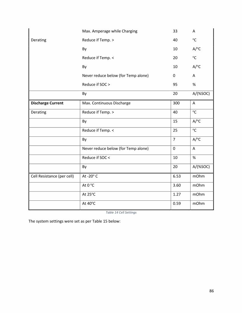
86
Max. Amperage while Charging 33 A
Derating Reduce if Temp. > 40 oC
By 10 A/oC
Reduce if Temp. < 20 oC
By 10 A/oC
Never reduce below (for Temp alone) 0 A
Reduce if SOC > 95 %
By 20 A/(%SOC)
Discharge Current Max. Continuous Discharge 300 A
Derating Reduce if Temp. > 40 oC
By 15 A/oC
Reduce if Temp. < 25 oC
By 7 A/oC
Never reduce below (for Temp alone) 0 A
Reduce if SOC < 10 %
By 20 A/(%SOC)
Cell Resistance (per cell) At -20o C 6.53 mOhm
At 0 oC 3.60 mOhm
At 25oC 1.27 mOhm
At 40oC 0.59 mOhm
Table 14 Cell Settings
The system settings were set as per Table 15 below:

87
Settings Descriptor Value Units
Current Sensor LEM S/24 500 A
Multi-Purpose I/P Function Keep-Awake -
Multi-Purpose O/P Function Err Signal Output
Invert Multi_purpose Output Polarity No
Pack Amp Hours 100 Ah
Current Sensor Polarity inverted No -
Always on Power Not Used Yes -
Charger Safety Relay Activated? Yes -
Trip if pack current exceeds CCL by 30 %
Max time relay stays on 600 min
Charge Enable Relay Activated? No -
Discharge Enable Activated? No -
Thermal Settings Active Thermistors 2,3,4 -
Intake Air Thermistor None -
Enable Fan Control Circuit No
Fault Settings Isolation Fault Detection Circuit Ignore -
Fault when ‘Charge’ AND ‘Ready’ power on Yes -
Fatal error if |Vpacksensor – ΣVcelltaps|> 101 V
Table 15 General Settings (Orion BMS)
From the profile wizard, the cell resistance profile is loaded based on testing done at Orion. The
resistivity map compared to temperature of a cell can be seen in figure 56, which is used to compensate
for changes in the cells internal resistance and thus output.

88
Figure 56 Cell Temperature Compensation
4.2.4 Rinehart 150 DX inverter Settings The inverter converters the DC battery power to useable AC motor power. As Highlighted in the
prototype specifications, it has a maximum rating of 150kW at 360Vdc. Rinehart supports the customer
with a large amount of documentation including a software user manual and calibration document –
thus only an overview of the calibration is required, with the settings that were programmed. Also
provided is a general ‘road-map’ to completion for the inverter supplied by Rinehart, which has been
adapted for HiCEV in figure 57 to show sections relevant to either calibration or commissioning. To
prepare the PC for connecting to the inverter the following downloads are required:
1. Tools
a. C2Proog
b. RMS GUI
2. Files
a. RMS GUI Library File
b. Latest Firmware files
c. Documentation

89
Commissioning
Calibration
Download all files and programs
Connect 12V Wiring, RS232, program switch and CAN to RMS unit
Start RMS GUI-Check Firmware
Test Program-enable switch and C2Proog
work by programming firmware
Connect HV cables
Program the Correct motor Type in the
EEPROM
Resolver calibration
Select EEPROM
1
2
3
4
5
6
7
8
Figure 57 Inverter Calibration steps
Connecting to the inverter requires connecting the 12V power, RS232 and program enable switch at a
bare minimum. The wiring diagram in Appendix 7.3 and the inverter loom mapping table in Appendix 7.4
gives the inverter pinout connections and the Rinehart suggested connectors, the inverter loom in figure
58 was created based off this information.

90
Figure 58 inverter wiring loom - final sizing
There are seven plugs in total; 2x Inverter connectors, SmartCraft (CANbus and 12V power), Resolver,
DC Power Supply (for bench programming) and SCI (RS232). The loom shown is the final loom lengths, as
during programing the lengths were an excessive length then reduced once the component approximate
lengths had been measured.
The 150DX differs from the EVCM, Eltek and the BMS as SCI (RS232) is used to program the module,
whereas CAN is used for control and feedback during operation. This is highlighted in figure 59 below
where the two PC utility tools are also shown; C2Proog and the RMS GUI are both broadcast over RS232.
PC
C2Proog
RMS GUI
Inverter Memory
RMS Firmware
RMS EEPROM
RS232
Figure 59 Firmware and EEPROM programming inverter over SCI
C2Proog updates the inverter firmware of the inverter in hex file format. The release of new firmware
depends on New Requests, Change requests and system bugs. An example of this is a new request for
motor parameters for a motor not previously integrated with the inverter.
The RMS GUI is required to setup the correct inverter parameters, which is loaded into the inverter
EEPROM. A snapshot of the RMS GUI EEPROM values is given in figure 60, where Motor_Type_EEPROM
= 36 represents the Remy HVH 250 115-PO motor and both Gamma_Adjust_EEPROM and
Resolver_PWM_Delay_EEPROM_(Counts) are set during the resolver calibration.

91
Figure 60 Snapshot of RMS GUI EEPROM parameters
Worth noting is that Inv_Cmd_Mode_EEPROM(CAN=0_VSM=1) is set to ‘0’ representing the EVCM
controlling the inverter though CAN and CAN_Bit_Rate_EEPROM is set to 250 kpbs. Also, although the
EVCM provides the platform for programming parameters, if the thresholds are not set more liberally in
the inverter EEPROM than the EVCM, the inverter EEPROM values become the limiting thresholds. The
below values in Table 16 from the inverter EEPROM are essential to vehicle performance as it was
discovered that regenerative braking was not working as the Regen_Torque_Limit_EEPROM was set to
‘0’, even though it was programmed higher at the EVCM.
Parameter EEPROM Value Physical Value Unit
IQ_Limit_EEPROM_(Amps)_x_10 5300 530 A
ID_Limit_EEPROM_(Amps)_x_10 5300 530 A
DC_Volt_Limit_EEPROM_(V)_x_10 3900 390 V
DC_UnderVolt_Limit_EEPROM_(V)_x_10 2500 250 V
Motor_Torque_Limit_EEPROM_(Nm)_x_10 3300 330 Nm
Regen_Torque_Limit_EEPROM_(Nm)_x_10 2000 200 Nm
Table 16 Inverter EEPROM – HV Power
The current limiting parameters; IQ_Limit_EEPROM_(Amps)_x_10 and ID_Limit_EEPROM_(Amps)_x_10
represent the quadrature and direct current limits respectively, indicative of the 3 phasor currents
(through inverse Clarke transform, on the assumption that the scaling ‘2/3’ is used) current magnitude.
The DC voltage limits are based on limitations of the inverter and the battery pack. The upper voltage
limit (DC_Volt_Limit_EEPROM_(V)_x_10) is dictate both by the inverter upper voltage limit of 400Vdc

92
while operating and the battery cell voltage limits of 3.65V per cell while charging (regenerative
braking). Thus, a voltage of 390Vdc provides a margin of 10Vdc on the inverter limits while allowing a
0.4Vdc margin per cell. The lower voltage limit of 250Vdc is dictated primary by the battery cell
resistance, and the associated voltage sag at maximum discharge current. At 80% depth of discharge,
the average cell voltage will be 3.2Vdc unloaded, thus gives the lower limit of pack voltage of 345.6Vdc.
This entails that a discharge current of 450Adc will ‘sag’ the DC bus voltage to 250Vdc if the internal
resistance per cell is equal to approximately 2mΩ, which according to the BMS cell resistance profile is
at temperatures above 15oC.
Both the motor and generation torque limits (Motor_Torque_Limit_EEPROM_(Nm)_x_10 and
Regen_Torque_Limit_EEPROM_(Nm)_x_10 respectively) are based on the Remy HVH250 motor
performance curves and the motor constant. From the motor performance curves in Appendix 7.5 the
maximum torque is 425Nm at a current of 600Arms giving a motor constant of approximately 0.71 Nm/A,
thus for a current of 450Arms, developed torque is 320Nm. Thus a torque of 330 Nm max allows the user
to calibrate up to the maximum allowable torque in the EVCM, with a 10Nm buffer for safety. The
regenerative braking was set to 200Nm to start, this parameter may have to be altered to allow for
more breaking depending on the customer’s drive profile and how they want the breaking to feel.

93
4.3 Commissioning (Systems integration) The physical commissioning of HiCEV maintains the modular approach, but with increased focus on the
module subsystems. Effective systems integration relies on robust and effective subsystems, as
communication errors cause incorrect operation, leaking coolant reduces thermal capability of a module
or high voltage on the vehicle chassis represents poses a safety hazard. To commission each module, the
subsystems are first mapped at a fundamental level in a top down approach, before being tested and
assessed.
4.3.1 Motor Mechanical Development The motor commissioning can be broken down into four subsystems, all of which are mechanical based
as the electrical aspects are the focus of the inverter. These subsystems included the adapter shaft
assembly, adapter plate, motor cradle and the motor cooling. The system reliance flow diagram is
shown in figure 61 below:
Design Adapter shaft and Bearing housing
Machining of Shaft and Housing
Source Accessory components (Bearings)
CMM and CAD Transmission bell
housing
Laser Machined
Adapter PlateAdapter Shaft and Bearing
Housing
Motor Full motor cradle assembly one unit.
Motor Cradle
Lengths Measured (motor assembly, motor
mounts)
Plate machined: Cut, bent, welded
Shaft assembly fastened to cradle and fastened
in the vehicle
Assemble all shaft components
Cooling Circuit Specified
Components sourced and connected
Subsystem tests
Cooling
Performance Testing
Figure 61 Mechanical breakdown of motor requirements

94
The adapter shaft was machined by a third party and assembled in house. The prototyping of the
adapter shaft dictates that the shaft was to be machined from a piece of round solid 4140 machine
steel. Two pictures below in figure 62 show the machining of the shaft and final assembly post
anodizing.
Notable features of the shaft are the spigot ridge on the adapter shaft which is concentric with the
flywheel, and the recess in the end of the adapter shaft which supports the run-out bearing which
supports the end of the transmission shaft. The runout bearing (shown sitting on the bearing housing
above) also allows the transmission shaft to move at a different speed to the motor when the clutch is
disengaged.
A metal gasket from the original engine to bellhousing was utilized to create the bellhousing adapter
plate in figure 63. A CMM profile of the gasket provided the hole pattern for a CAD file to be constructed
accurately. This was of importance due to the accuracy required to align the adapter shaft to prevent
‘run out’. The center hole in the gasket is assumed (due to the difficulties associated with implementing
a dial indicator in an enclosed space) to be concentric with the transmission output shaft. The
transmission in
Figure 62 Adapter shaft machined

95
Figure 63 Bellhousing adapter plate
Figure 63 also displays how the adapter plate fastens to the transmission and the single aligning stud
protruding through the bellhousing plate. The motor cradle is welded to the adapter plate and has a
twofold purpose; to reduce the cantilever loading though supporting the motor from the rear and to
also support the entire transmission though motor assembly from the pre-existing motor mounts.
Figure 64 Motor Placement
The motor with lifting eyebolts in figure 64 above shows positioning of the motor, which was
subsequently removed and giving a red powder-coat coloring to prevent rust.
4.3.2 Inverter The inverter can be broken down to four base commissioning subsystem aspects; mechanical, low
voltage, high voltage and cooling. These subsystems and dependencies are shown below in figure 65 to
indicate the integration required to initiate performance testing of the inverter. Additionally, the red
highlighted section indicates the focus aspects with interfacing the motor with the inverter physically.

96
Align Inverter in engine bay (proximity to motor and HV protection box)
Machine mounting bracket
Create wiring looms from documentation
Route Looms
Low VoltageInverter Mechanical High Voltage
Cable Formed(Cut to length, Stripped,
lugged, heatshrink)
Lugs cut to fit motor
Align phases from inverter and motor
Connect powerBolt to Motor assembly
Resolver Calibration
Cooling Circuit Specified
Components sourced and connected
Cooling
Performance testing
Subsystem tests
Figure 65 Inverter subsystems
4.3.2.1 Interfacing with Remy HVH 250-115 PO
The selected motor for the driving force of HiCEV is the Remy HVH 250-115PO. This three phase oil
cooled motor utilizes a 5 rare earth magnetic pole pair rotor. The low voltage connection provides
analog rotor position and internal temperature information to the inverter. Accurate rotor position
information is required by the inverter DSP to implement effective switching.
4.3.2.2 Resolver
To effectively implement the output motor ac waveform, the inverter switching requires feedback in the
form of the rotor position. Remy utilized the resolver as a position sensor which employs a coil which is
supplied with a single frequency sin wave from an external source (the inverter). Another two coils are
arranged to be 90 electrical degrees out of phases with one another (equivalent to Sine and Cosine)
which is transmitted to the inverter decoding circuitry (arctangent function) to determine rotor position
[42] the arrangement of which can be seen in figure 69. These connections are prone to cross talk due
to the nature of induced waveforms and Remy claims to have implemented a strategy in the motor
internals to reduce the effects. Thus, to maintain a high level of accuracy through faraday shielding of
crosstalk on signal lines, twisted pair shielded cabling were utilized to connect between motor resolver
and inverter. The way the twisted pairs were arranged is shown in figure 70 with the pinouts of each
module on resolver end and inverter end, where the reference wiring diagram is shown in Appendix 7.3.

97
Motor Rotor
Shaft
Rotary TransformerSIN and COS windings
Reference winding
Figure 66 Example of brushless resolver
Figure 67 Electrical Circuit for rotary transformer resolver
It is assumed that a rotary transformer is utilized in the resolver to provide brushless operation, the
concept is shown in figure 70.
The calibration of the resolver is twofold; calibrate the inverter resolver delay from the resolver circuitry
(Resolver Delay) and adjust the offset between resolver and magnetic field of the motor (Gamma
Adjust). The aim of calibrating the resolver delay is to read the peak values of the SIN and COS position
Figure 68Wiring from resolver to inverter

98
waveforms, and thus maximizing the amplitude for the font end analog to digital converter to the DSP
[45].
The inverter resolver calibration took place in-situ on the farm. At the time of calibration, the battery
pack had not yet been placed in the vehicle and as such required an external aide to create rotation of
the motor shaft. A tractor was utilized to tow HiCEV while the motor was mechanically connected to the
drivetrain while parameters were read from the RMS GUI, shown in figure 72. The motor was allowed to
spin at speeds up to 4000 RPM during testing, allowing a B-EMF to be generated in the region of 100Vac
(based on a B-EMF co-efficient of 25.9 Vrms, line-line/krpm [remy application manual]) on the HVAC
connections to the inverter. The HVDC terminals were isolated during this calibration, a proportional
voltage is generated across the terminals equivalent to Vrms. line-line = 0.785 . VDC or 130Vdc. The parameter
DC_UnderVolt_Thres_EEPROM was set to ‘0’ in the RMS GUI to avoid the inverter producing an error
code with not battery voltage present on the HVDC terminals during these calibrations.
Resolver Delay
The initial calibrate the resolver delay, the motor requires cogging-torque discrete increments of
rotation. To achieve the smallest increment possible, the vehicle was placed into 2nd gear and pushed by
hand while monitoring the RMS GUI. The maximum value of COS resolver waveform
(Cos_corr_(V)_x_100 ) was found at a resolver delay (Resolver_Delay_Command) of 900 which was then
programmed into non-volatile memory (Resolver_PWM_Delay_EEPROM_(Counts)).
Resolver Direction
Direction of the resolver was verified to ensure that the resolver feedback correctly conveyed forward
motion of the vehicle. Rolling the vehicle forward increases electrical angle of the motor
(Gamma_Resolver_DEG_x_10) from 0 to 3600 then reset to 0 in the forward direction. Additionally,
feedback speed parameter (Feedback_Speed_(RPM)) indicates a positive value in forwards direction and
negative in reverse.
Physical wiring of motor phase connections also affect the motor direction. To verify correct phase
connections, motor B-EMF is observed by the inverter at a speed of 4000 RPM (VBEMF = 100Vrms, line-line)
where polarity of the voltage feedback speed from the B-EMF matches the direction of the resolver.
Gamma Adjust
Due to manufacturing tolerances, the resolver rotational position is not always in the same place or
aligned with the motor magnetic field. Similarly to resolver direction calibration, a sufficient B-EMF (and
thus motor speed) is required by the internal voltage sensors in the inverter to determine the alignment.
Figure 69 Resolver Test Setup

99
The angle between the B-EMF and the resolver (Delta_Resolver_In_Fil_(DEG)_x_10) is required to be a
constant value of Ө= 90 ±2o (900 in the RMS GUI) when rotating in the forward direction. The
difference between the current delta angle and 90o is used to alter the current calibration angle
between resolver and motor BEMF (Gamma_Adjust_(Deg)_x_10). An increase in calibration angle gives
a decrease in resolver angle, thus if the resolver angle is higher than desired (Ө > 90o), the calibration
angle is increased to converge on 90o.
Ө𝛾+1 = Ө𝛾 − (90 − Ө∆)
Thus the new resolver
Ө∆+1=Ө∆ - Ө𝛾+1
This is an iterative process to converge on Ө∆+1= 90o whereby the final calibration angle Ө𝛾+1 is
programmed (Ө𝛾𝑒 = Ө𝛾+1) into the EEPROM (GAMMA_Adjust_EEPROM_(Deg)_x_10). This yielded a
calibration angle of Ө𝛾𝑒 = 109.4o or similarly, GAMMA_Adjust_EEPROM_(Deg)_x_10 = 1094.
4.3.2.3 HV Safety Circuit
Health and safety must be at the forefront of design, eliminating hazards where possible and failing
that- mitigation. There are two major consequence scenarios; economic damage to property and
damage to people. High voltage is the most obvious risk associated with an electric vehicle, it is has the
highest presence in operating or working on the vehicle in terms of exposure. High voltage is required
for vehicle operation, thus mitigation techniques to reduce consequence have been employed. These
are explored below:
1. Visual indicators of HV
a. Orange insulation is used primary possible
b. Orange conduit is used as a substitute where cabling of certain sizes are not readily
available with orange insulation
c. Appropriate signage
2. Safety Electronics
a. Mandatory fusing on all HV circuits
b. HV rated relays and switches
i. Dual Pole Isolation
c. Sealed enclosures to eliminate exposed HV surfaces and connectors
d. HV sensors on the BMS and inverter
3. Proximity
a. Ensuring HV cabling lengths are kept short
b. The two HVDC poles from the battery pack are kept apart to reduce chance of shorting
during common cable failure
c. Accessibility of HV electronics
d. Cable guarding HV cables under the vehicle

100
Safety Electronics
The main battery fuse specifications are shown in the
Battery Characteristics Bussman Fuse
Op Voltage
(Vdc)
Resistance
(mOhm)
Short Circuit
Current (A)
K Factor I2t K* I2t (A.s2) t (ms)
360 100 3500 0.61 149000 90890 7
The HV safety wiring schematic is shown below in figure 70, where the physical HV Battery saftey box is
shown in figure 71.
Figure 70 HV Safety Wiring

101
Figure 71 Physical HV Main Safety
The HV Safety Circuit consisted of the Pre-charge circuitry and the HV Main battery protection circuitry.
The pre-charge circuit is shown below in figure 73 and the physical wiring the the safety elements in the
HV circuit is shown in figure 74.
Pre-charge Parameter Value Unit Description
R 600 ohm
C 500 uF
taw 0.3 s
#Constants 3 # Number of constants
t 0.9 s 3 time constants
exp(-t/taw) 0.049787
Vo 340 V
V(t) 323.0724 V 95.02129 % % of max voltage
Energy 26.09394 J Energy in Cap
Q 0.161536 C Charge
Fc 0.530516 Hz Cut-off Freq Figure 72 Pre-Charge component validation
Auxiliary Fuses
Battery Fuse
Main Contactor
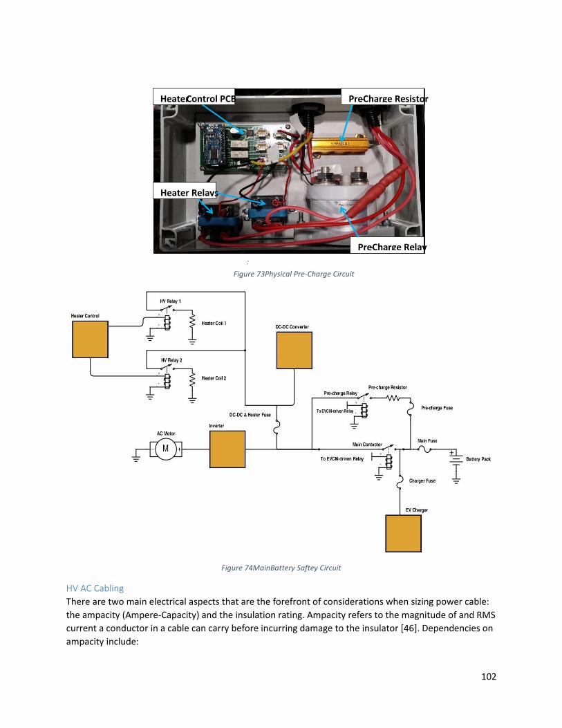
102
Figure 74MainBattery Saftey Circuit
HV AC Cabling
There are two main electrical aspects that are the forefront of considerations when sizing power cable:
the ampacity (Ampere-Capacity) and the insulation rating. Ampacity refers to the magnitude of and RMS
current a conductor in a cable can carry before incurring damage to the insulator [46]. Dependencies on
ampacity include:
:
Heater Control PCB
Pre - Charge Relay
Pre - Charge Resistor
Heater Relays
Figure 73Physical Pre-Charge Circuit

103
Insulation temperature rating
Electrical resistance of conductor
AC Frequency
Thermal conductivity of insulation
Ambient temperature
Humidity
Insulation ratings refers to both electrical and environmental ratings such as;
Dielectric breakdown
Resistance to corrosive substances
Ozone resistance
Weathering resistance
Flame retardant
As a result, 95mm2 Radox screened battery cable was sourced for the inverter connections which has
the following properties:
Parameter Value Unit
Voltage Rating 600 Vac
Temperature Rating -55 to 150 oC
Conductor cross section 95 mm2
Amacity 200A at 75oC [47]
Conductor - ISO 6722
Conductor - DIN EN 13602
General – ISO 6722 class D, thin wall (Appendix
7.6)
General – LV216
Figure 75 HV Cable Specifications
Where Appendix 7.6 gives the specifications for ISO 6722 Class D, which covers thermal capacities,
exposure to weathering and common automotive fluids [48]
With regards to the electrical specifications, the insulation needs to not undergo dielectric breakdown
from the carrying voltage. If this is adhered to, the current carrying capability of the wire (ampicity)
should be as large as possible to reduce the voltage drop per unit length along the cable. The ampacity
of the cable is essentially related to the diameter of the power carrying core and the material (usually
copper or aluminum). The diameter of the cable should be as large as possible to reduce the resistance
and thus heat dissipation per unit length of the cable, but there may be constraints such as; maximum
cable gland OD fittings on the HV modules, bend radius for space between modules or cost.

104
The Meger test results conducted by the undergraduate students are given below in table , showing
cable insulation is in working condition.
Cable Section Insulation Resistance
Battery to Protection DC+ >1000MΩ
Battery to Protection DC- >1000MΩ
Protection to Inverter DC+ >1000MΩ
Protection to Inverter DC- >1000MΩ
Inverter to Motor A >1000MΩ
Inverter to Motor B >1000MΩ
Inverter to Motor C >1000MΩ
Figure 76 Meger test results on HV Cable
In figure 68 below is the megger test completed by each cable and the HV Motor leads that had to have
modifications to the lugs to fit on the motor connections.
Figure diagram expands on the physical HV diagrams above and shows the HV routing though to the
battery boxes also.
Figure 77HV Cable meger tests and Motor Connections

105
HVDC Relay
HVDC+ to Inverter
HVDC- o Inverter
HVDC Fuse
Inverter
HVDC- to Batt
HVDC+ to Batt
Braided interconnects
Cable Lugs
Battery Lug
Re
sistor
Fuse
He
ater con
trol P
CB
Heater Control Relay 1
Heater Control Relay 2
Cabin Heater PTC
1
Cabin Heater PTC
2
HV
DC
10A
DC
DC
& H
eater
Fuse
HVDC 5A Pre-Charge Fuse
HV
DC
Re
lay
HV
DC
10
A C
harge
r
VCM
DCDC Converter
HVDC+ to Inverter
HVDC+ to Inverter
HVDC+ to Inverter
HVDC+ to Inverter
HVDC+ to Inverter
HVDC+ to Inverter
HVDC+ to Inverter
HVDC+ to Inverter
HVDC+ to Inverter
Ch
arge
r
HVDC+ to Inverter
Figure 78 HV Battery cable wiring

106
4.3.3 CANbus CANbus was created from twisted pair cable with grounds of each module all connected via the
shielding to provide a common reference ground for all transceivers.
4.3.3.1 CANbus Database
A database of CAN messages was compiled for HiCEV and is shown below in table 17:
Message ID DLC Speed Origin Destination Endian Definitions Timeout
Threshold
Hex Dec (ms)
Sec ( = Tx
speed x 2)
A0 160 8 100 Inverter VCM Little
Temperatures #1 -
IGBT's, Gate driver 0.2
A1 161 8 100 Inverter VCM Little
Temperatures #2 -
Control Board, RTD's 0.2
A2 162 8 100 Inverter VCM Little
Temperatures #3
RTDS, Motor /
Torque Shudder 0.2
A3 163 8 10 Inverter VCM Little
Analog Input
Voltages 0.02
A4 164 8 10 Inverter VCM Little Digital Input Status 0.02
A5 165 8 10 Inverter VCM Little
Motor Position
Information 0.02
A6 166 8 10 Inverter VCM Little
HV Voltage
information 0.02
A7 167 8 10 Inverter VCM Little
Flux Information
(Control and
feedback) 0.02
A8 168 8 10 Inverter VCM Little
Internal Reference
Voltages 0.02
A9 169 8 100 Inverter VCM Little Internal States 0.2
AA 170 8 100 Inverter VCM Little Fault Codes 0.2
AB 171 8 10 Inverter VCM Little 0.02
AC 172 8 10 Inverter VCM Little
Torque and Timer
Information 0.02

107
AD 173 8 10 Inverter VCM Little
Modulation Index /
Flux Weakening
Output 0.02
AE 174 8 100 Inverter VCM Little
Firmware
Information 0.2
AF 175 Diagnostic Data
C0 192 8 20 VCM Inverter Little
Command Message:
Inverter Lockout
Enable 0.04
C1 193 PC Inverter
Write/Read a
Parameter (Byte 2 =
1/0 respectively)
C2 194 Inverter PC
Response message
from this
101 257 8 45 BMS VCM Big 0.09
102 258 8 45 BMS VCM Big 0.09
103 259 6 20 BMS VCM Big 0.04
104 260 8 450 BMS VCM Big 0.9
106 262 1 90 BMS VCM Big 0.18
Table 17 CANbus Message Database
4.3.4 Battery Pack The battery pack state of charge was unknown before putting it in the vehicle, as the cells hold a
constant voltage over 80% of the operating region. Tests were conducted to test charger and BMS
would charge the batteries before were placed in the vehicle.
BMS
The test layout was such that, a resistive load was put across the bank while monitoring the current
manually by means of current clamps to compare against the BMS readout

108
Batteries
The battery pack consists of sections; batteries, enclosure and layout, connectors and BMS connections.
Prototype specifying outlined the chosen battery pack as 108 Winston 100Ahr Lithium Ion batteries, and
the enclosure as a 3mm aluminum box with detachable lid. Before the batteries were placed in the
vehicle, since accessibility in and out of the vehicle is limited (about a day long process to remove the
battery batteries, cabling and the enclosure) testing to ensure the BMS and charger interfaced correctly
to both charge and monitor the batteries effectively was crucial.

109
4.3.4.1 Initial BMS Setup
The initial BMS taps connections were loose and resulted in the variations in voltage and resistance as
shown below in the voltage test and the corresponding resistance profile spread. Tightening the taps
would usually bring the resistance down to the 15mΩ operating region.
-15
-10
-5
0
5
10
15
20
25
2
2.2
2.4
2.6
2.8
3
3.2
3.4
3.6
3.8
1 3 5 7 9
11
13
15
17
19
21
23
25
27
29
31
33
35
37
39
41
43
45
Pac
k C
urr
ent
(A)
Cel
l Vo
ltag
e (V
)
Time (s)
Cell Voltage Test

110
4.3.5 Vehicle Analysis Two drive scenarios were explored with the aim of proving that retaining the gearbox has performance
benefits over a directly coupled shaft. The gear selected to conduct the comparison was third, where
either Fourth or third gear could have been selected to simulate the directly coupled drive due to the
ease of changing the rear differential ratio. The speedometer was out of service so a GPS system was
utilized to indicate that the vehicle was traveling 100 km/hr. at which point the accelerator was abruptly
released to indicate the target had been met (current tends to 0).
To allow for a valid comparison between the two drive scenarios, the following tests were conducted
with the following conditions:
The same driver used in both tests
A common starting position
Relatively even surface tar seal that was safe to use
On the same day (Same weather conditions)
Rear-wheel driven (not in 4WD)
100% Accelerator input
1.5
2
2.5
3
3.5
4
4.5
5
5.5
6
1 2 3 4 5 6 7 8 9 10 11 12 13 14 15 16 17 18
Cel
l Res
ista
nce
(m
Ω)
Time (s)
Cell Resistance Profile
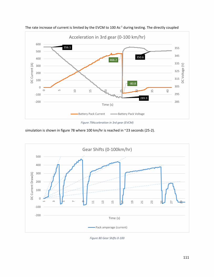
111
The rate increase of current is limited by the EVCM to 100 As-1 during testing. The directly coupled
simulation is shown in figure 78 where 100 km/hr is reached in ~23 seconds (25-2).
Figure 80 Gear Shifts 0-100
-200
-100
0
100
200
300
400
500
1 3 5 7 9
11
13
15
17
19
21
23
25
27
29
DC
Cu
rren
t D
raw
(A)
Time (s)
Gear Shifts (0-100km/hr)
Pack amperage (current)
466.2
-80.8
356.1
289.9
350.6
285
295
305
315
325
335
345
355
-200
-100
0
100
200
300
400
500
6000 5
10
15
20
25
30
35
40
DC
Vo
ltag
e (V
)
DC
Cu
rren
t (A
)
Time (s)
Acceleration in 3rd gear (0-100 km/hr)
Battery Pack Current Battery Pack Voltage
Figure 79Acceleration in 3rd gear (EVCM)

112
Shifting gears in the above figure 79 takes between 1.4-1.7 seconds, which gives approximately 6
seconds lost to shifting. Accelerating stopped at 25 seconds at the end of 4th gear, which is 2 seconds
slower than fixed gear. Although the gear shifting is slower getting to 100 km/hr, the torques that are
able to be developed with the low gearing allow the gear shifting scenario to attain 435A in 3rd gear 3
seconds faster than the fixed gear. Reducing the time from 0-100 km/hr could be done by implementing
the clutch switch so regenerative braking doesn’t occur during shifting, relaxing the thresholds of rate
limiting on the battery current, reducing vehicle weight from the deck boards, a bash panel lining the
engine bay to decrease the drag force, decreasing the shifting times, shifting to third and staying there
or putting the vehicle in 4WD to reduce slip. Implementing the above changes, will increase the
likelyhood of attaining the <12s to accelerate from 0-60mph performance standard.
Additional energy and power information can be taken from figure 78 Peak power draw is ~135kW and
uses 1.6MJ of energy (1.3% of SOC) (J=(Vav*Iav/2)*22) Vav*Iav = 75kW. The current regenerative breaking
settings ~6% energy was recaptured (~100kj = 356Vdc*40A*7sec).
The total dc system resistance is (@point 18) (Rtot = 356-300/400 = 140mΩ = ~1.25mΩ per cell)
Towing a tractor simulated towing a 2 tonne trailer, which is standard for the work vehicles. To tow the
Tractor at 10 km/hr in first gear, the battery current required is 50Adc which gives a required power of
17.650 kW which gives an average operation time of approximately 2 hours. Switching to second gear at
25 second point reduces the current draw to 40A and thus an average power draw to 14kW or a 2.5
hour run time. An assumption made in these summary calculations is zero road grade, which will
significantly effect the power draw and thus run time.
Figure 81 Towing tractor at 10km/hr
344
346
348
350
352
354
356
358
360
-30
-20
-10
0
10
20
30
40
50
60
0 2 3 4 5 6 7 8 9
10
11
12
13
14
15
16
17
18
19
20
21
22
23
24
25
26
27
28
29
30 D
C V
ola
tge
(V)
DC
Cu
rren
t (A
)
Time (s)
Towing tractor at 10 km/hr
Pack amperage (current) Pack voltage

113
Figure 82Acceleration to 80km/hr
The above figure 81 shows a total loss of 11% SOC over a 21 second acceleration. Vav = 345Vdc
Voltage dc,av (V) Current dc, average (A) Time (s) Energy(kJ)
1st gear 345 80 5 138
2nd gear 345 100 4.5 155
3rd gear 345 100 4 138
4th gear 345 100 6.5 224
Total 655 Table 18 Energy consumed through different gears
Which yields a decrease in SOC in the order of 0.5% from table 18, therefore is being misinterpreted by a
factor of 20.
4.3.6 Cooling The temperature for the inverter and motor require constant monitoring to ensure safe operating
regions are always being operated in. The upper threshold temperatures for these two components are
160oC and 105oC for the motor and inverter respectively. Thermal limitations are put in place to limit
current to zero at 140oC and 80oC for the motor and inverter respectively should the liquid cooling loops
be insufficient or fail. An example of the temperature reached from the inverter and motor combination
over a short, but intensive discharge current (480A) below in figure 82.The figure shows the motor has a
higher thermal inertia than the inverter, thus takes longer to respond to changes in temperature. This
can be depicted both in the initial spike in inverter module ‘D’ temperature from 28 to 39oC (over 28
seconds and a decrease from 48.6 to 40.7oC (change of 8oC) in 18 seconds.
0
10
20
30
40
50
-100
-50
0
50
100
150
200
250
0 2 3 4 5 6 7 8 9
10
11
12
13
14
15
16
17
18
19
20
21
22
23
24
25
SOC
(%
)
DC
Cu
rren
t (D
C)
Time (s)
Acceleration to 80 km/hr
Pack State of Charge Amp Hours

114
Figure 83Inverter and motor Thermal profile
Figure 84Thermal paste effects on charger
During charging, the Eltek charger dissipates a maximum of 220W of heat. Figure 83 shows that the
thermal past reduces heat conduction away from the charger at higher temperatures by 2oC
approximately 50oC operating temperature on the primary sensor.
0
10
20
30
40
50
60
-200
-100
0
100
200
300
400
500
600
0
10
20
30
40
50
60
70
80
90
10
0
11
0
12
0
13
0
14
0
15
0
16
0
17
0
18
0
19
0
20
0
21
0
22
0
23
0
24
0
25
0
26
0
DC
Cu
rren
t (A
)
Time (s)
Module Temperature under Load
BattCur D2_Module_B D3_Motor_Temperature
y = -5E-08x2 + 0.002x + 34.779
y = -3E-08x2 + 0.0018x + 34.587
25
30
35
40
45
50
55
0
10
20
30
40
50
60
70
80
90
10
0
11
0
12
0
13
0
14
0
15
0
16
0
17
0
18
0
19
0
Ch
arge
r Te
mp
(D
egC
)
Charge Time (Min)
Effect of Thermal Paste During Charging
Primary Temp (No) Secondary Temp (No) Primary Temp (Yes)
Secondary Temp (Yes) Poly. (Primary Temp (No)) Poly. (Primary Temp (Yes))

115
5.0 Discussion This project covered many different aspects of engineering, project, electrical and mechanical. The vehicle is now in a state where it can be driven and tested.
5.1 Issues Faced All major components except the DCDC converter were sourced from different countries. The support
was less than favorable when issues with components arose, and it is difficult or impossible to remedy a
solution if communications fail. Two companies that were used to source components from gave wrong
specifications and sent wrong products, contributing to massive delays in commissioning. A 3 month
delay occurred when the wrong batteries were sent, which left the team waiting for the right set to be
sent.
Documentation for the EVCM also fell short as to what was expected –wiring the EVCM was on hold for
months as no wiring diagram was supplied with the module, step through initiation documents to setup
parameters once in MotoTune or reference documentation for the hundreds of variables in MotoTune.
Contact was finally made with the company months after issues were raised.
Although these issues were significant hurdles, it gave insight into detailing crucial project elements
regarding. The issue with documentation should have been sorted before purchasing took place.
Diligence is paramount when dealing with companies based in other countries – as the inclination to
have good customer rapport seems to be less than when both parties are on the same continent.
5.2 Future for HiCEV HiCEV requires refining and general tidying of systems. The project is currently at a phase where the
systems can be tested safely as cooling is being used and lubrication in the motor bearings.
The aim for the undergraduate student project this year is twofold; certification of the vehicle to meet
the LVVTA standards and refining of vehicle system performance.
6.0 Conclusion The aim of this project was to design and prototype a high country electric vehicle (HiCEV) for farming
applications. HiCEV was the result of a farmers desire to reduce his farms dependency on fossil fuels and
to promote electric vehicles in the agricultural sector of NZ.
The prototype specification design converged on the solution of a single electric motor, coupled to the
pre-existing manual gearbox. The core of this build is a robust IPM motor driven by a FOC inverter and
EVCM controller.
Development of the prototype has reached the state where commissioning main systems of motor,
inverter and battery management has been completed and performance testing is starting to
commence. Further work will be in finishing the subsystems integration, programming the EVCM
performance parameters and aiming for certification of the vehicle by the end of the year.

116
7.0 Appendix
7.1 Birds eye view of component layout

117
7.2 CAD model of battery boxes
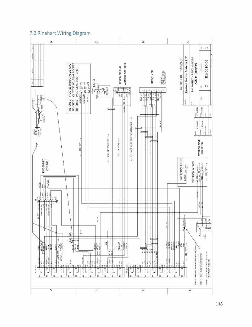
118
7.3 Rinehart Wiring Diagram

119
7.4 Inverter Loom Mapping

120
Origin Header
Connector
Type
Pin
# Pin Name Description Destination Component
End
Pin
#
Cable size
(AWG)
Cable
Description
Est.
Length
(m)
Used
Inverter J1 770854-1 1 XDCR_PWR +5V @ 80mA max No
13 AIN1 Analog Input 1 0-
5VFS, Accelerator No
24 AIN2 Analog Input 2 0-
5VFS
Motor Resolver Header,
Temp Sens G 16-20
Multi Core
Shielded 1.5 Yes
2 AGND Analog Ground Motor Resolver Header,
ANGD H 16-20
Multi Core
Shielded 1.5 Yes
14 XDCR_PWR +5V @ 80mA max No
25 AIN3 Analog Input 3 0-
5VFS, Brake No
3 AIN4
Analog Input 4 0-
5VFS, Not
assigned
No
15 AGND Analog Ground No
26 XDCR_PWR +5V @ 80mA max Inverter, AIN2 (resolver
connection), w Resistor -- 16-20
Multi Core
Shielded 1.5 Yes
4 AOUT Analog Output (0
– 5V) No
16 AIN6 Analog Input 6 0-
5VFS No
27 RLY6 High-side Relay
Driver No
5 RTD1 PT100 or PT1000
RTD No
17 AGND Analog Ground No
28 XDCR_PWR 5V @80mA max No
6 RTD2 PT100 or PT1000
RTD No
18 AIN5 Analog Input 6 0-
5VFS No
29 RLY5 High-side Relay
Driver No
7 /PROG_ENA Serial Boot Loader
enable
PROGRAMING,
DB9,RS232 5 16-20
Yellow, single
core 2 yes
19 AGND Analog Ground No
30 DIN1 Digital Input 1 –
STG(1) No
8 DIN2 Digital Input 2 -
STG No
20 DIN3 Digital Input 3 -
STG No
31 DIN4 Digital Input 4 -
STG No
9 DIN5 Digital Input 5 –
STB(2) No
21 DIN6 Digital Input 6 -
STB No
32 DIN7 Digital Input 7 -
STB No
10 DIN8 Digital Input 8 -
STB No

121
22 GND Ground PROGRAMING,
DB9,RS232 | CANA Shield 5 16-20
Black (green),
single core 2 yes
33 CANA_H CAN Channel A Hi J3, DB9 7 16-20 Shielded, Twisted
Pair 0.3 yes
11 CANA_L CAN Channel A
Low J3, DB10 2 16-20
Shielded, Twisted
Pair 0.3 yes
23 CANB_H CAN Channel B Hi No
34 CANB_L
CAN Channel B
Low RS-232
Transmit
No
12 TXD RS-232 Receive PROGRAMING,
DB9,RS232 2 16-20
Orange, Single
core, multi
strand
2 Yes
35 RXD RS-232 Transmit PROGRAMING,
DB9,RS232 3 16-20
Tan, Single core,
Multi strand 2 Yes
J2 770854-1 1 XDCR_PWR +5V @ 80mA max
9 No
9 ENCA Encoder Channel A
input No
16 ENCB Encoder Channel B
input No
2 ENCZ Encoder Channel Z
input (Index) No
10 GND GND No
17 EXC Resolver
excitation output Motor Resolver B 16-20
Shielded, Twisted
Pair, red collar 1.5 Yes
3 EXC_RTN EXC_RTN Resolver
excitation return Motor Resolver A 16-20
Shielded, Twisted
Pair, red collar 1.5 Yes
11 SIN Resolver Sine
winding + Motor Resolver C 16-20
Shielded, Twisted
Pair, green collar 1.5 Yes
18 /SIN Resolver Sine
winding - Motor Resolver E 16-20
Shielded, Twisted
Pair, green collar 1.5 Yes
4 COS Resolver Cosine
winding + Motor Resolver D 16-20
Shielded, Twisted
Pair, blue collar 1.5 Yes
12 /COS Resolver Cosine
winding - Motor Resolver F 16-20
Shielded, Twisted
Pair, blue collar 1.5 Yes
19 SHIELD Resolver Shield Motor Resolver J 16-20 Shielded, Twisted
Pair, bare 1.5 Yes
5 HALL_A Hall Encoder Chan,
A No
13 HALL_B Hall Encoder Chan,
B No
20 HALL_C Hall Encoder Chan,
C No
6 GND Main 12V return 12V Return / Vehicle
Chassis GND 16-20
black, single
strand 0.3 Yes
14 GND Main 12V return Relay GND GND 16-20 black, single
strand 0.3 Yes
21 RLY1 Hi-Side Relay
Driver Precharge relay driver + 16-20
green, single
strand 0.5 Yes
7 RLY2 Hi-Side Relay
Driver Main Relay Drive + 16-20
yellow, single
strand 0.5 Yes
15 RLY3 Lo-Side Relay
Driver 16-20
blue, single
strand 0.5 Yes

122
22 RLY4 Lo-Side Relay
Driver 16-20
brown, single
core Yes
8 BATT+ Main 12V power
source
12V Main PWR (batt),
switched Batt 16-20 Red, dual core 0.3 Yes
23 BATT+ Main 12V power
source
12V Main PWR (batt),
switched Batt 16-20 0.3 yes
23 CANB_H CAN Channel B Hi 16-20 no

123
7.5 Motor Performance Diagrams

124
7.6 Class D Specifications Section Description Requirement
5.7 Insulation Volume Resistivity 109 Ω /mm min.
5.8 Pressure at High Temperature ‘0.8N @150°C no dielectric breakdown
5.9 Strip Force / Adhesion Per customer agreement
5.10 Low Temperature Winding 3 tns 2.5kg - 40°C no dielectric breakdown
5.11 Impact 100gm @-40°C no breakdown
5.12.4.1 Sandpaper Abrasion .2kg 350mm min
5.12.4.2 Scrape Abrasion Per customer agreement
5.13 Long-Term Heat Aging 150°C 3000 hours
5.15 Thermal Overload 200°C 6 hours
5.16 Shrinkage by heat 2mm max. 150°C
5.17 Fluid Compatibility
Gasoline 15% max.
Diesel Fuel 15% max.
Engine Oil 15% max.
Ethanol 15% max.
Power Steering 30% max
Automatic Transmission 25% max.
Engine Coolant 15% max
Battery Acid no breakdown
5.19 Ozone Resistance 45°C 85% Relative Humidity 70
hours, Ozone 50 +/- 5 pphm
1kV 1 min. (no breakdown)
5.20 Resistance to hot water not less than 10-5 ohm-mm
5.21 Temperature /Humidity Cycling 40 - 8 hours cycles -40°C and 125°C 80 -
100% relative humidity
5.22 Resistance to Flame
Propagation
70 sec. max. 50mm unburned
Diesel Fuel 15% max.

125
Engine Oil 15% max.
Ethanol 15% max.
Power Steering 30% max

126
8.0 Bibliography
[1] M. Ramsey, "Wall Street Journal," [Online]. Available: http://www.wsj.com/articles/aston-martin-
may-build-electric-rapide-sports-car-in-2-3-years-1427744700.
[2] Tesla Motors, "Tesla Motors," [Online]. Available: http://www.teslamotors.com/models.
[3] "Hitachi Construction Machinery - Americas," [Online]. Available:
http://hitachiconstruction.com/eh3500acii.html.
[4] John Deere, "John Deere, 644K Hybrid Wheel Loader," [Online]. Available:
https://www.deere.com/en_US/products/equipment/wheel_loaders/644k_hybrid/644k_hybrid.pa
ge?.
[5] "FIA Formula-e Championship," [Online]. Available:
http://www.fiaformulae.com/en/guide/overview.aspx.
[6] "Glenthorne Station," [Online]. Available: http://www.glenthorne.co.nz/recreational-
activities/station-to-station-tramps.
[7] "EECA energywise," [Online]. Available: http://www.energywise.govt.nz/your-vehicle/new-
technologies/electric-vehicles.
[8] M. A. M. a. D. W. G. Chris Mi, "HYBRID ELECTRIC VEHICLES," in Principals and Applications with
Practical Perspectives, Wiley, 2011, p. 470.
[9] "Drive Electric," [Online]. Available: http://driveelectric.org.nz/.
[1
0]
"Ministry of Transport," [Online]. Available:
http://www.transport.govt.nz/assets/Uploads/Research/Documents/2013-Fleet-report-final.pdf.
[1
1]
"EECA," [Online]. Available: https://www.energywise.govt.nz/on-the-road/electric-vehicles/.
[1
2]
U. o. Waikato, "Energy Infomatics," [Online]. Available:
http://ei.cms.waikato.ac.nz/index.php/projects/v2g/.
[1
3]
"Ministry of Transport," [Online]. Available:
http://www.transport.govt.nz/research/othertransportresearch/electricvehicles/.
[1
4]
R. Cho, "PHYS.ORG," [Online]. Available: http://phys.org/news/2015-06-batteries.html.

127
[1
5]
"Air New Zealand," [Online]. Available: http://www.airnewzealand.co.nz/press-release-2016-air-
new-zealand-electrifies-ground-fleet.
[1
6]
U. o. Michigan, "Center for Sustainable Systems," [Online]. Available:
http://css.snre.umich.edu/css_doc/CSS01-07.pdf.
[1
7]
D. Wratt, "NIWA," [Online]. Available: https://www.niwa.co.nz/our-science/climate/information-
and-resources/clivar/greenhouse.
[1
8]
S. L. Dr Allan Miller, "Electric Vehicles in New Zealand," [Online]. Available:
http://www.theenergyconference.org.nz/uploads/98897/files/Presentations/Allan_Miller___Scott_
Lemon.pdf.
[1
9]
"U.S. Energy Information Administration," [Online]. Available:
https://www.eia.gov/energyexplained/index.cfm?page=electricity_home.
[2
0]
"Washington University," [Online]. Available: http://courses.washington.edu/me341/oct22v2.htm.
[2
1]
R. R. Gerhold, "Houston Electric Auto Association," [Online]. Available: http://heaa.org/wp-
content/uploads/library/DC_vs_AC_motors.pdf.
[2
2]
M.S.May, "Helwig Carbon Products," [Online]. Available:
http://www.helwigcarbon.com/assets/files/pdf/Articles/ta1_96_2013%20brushes_sprkng_mach%2
0maint%20single%20pages.pdf.
[2
3]
"Engineering 360," [Online]. Available:
http://www.globalspec.com/reference/10796/179909/chapter-3-ac-and-dc-motors-ac-motors-
enclosure-types-and-cooling.
[2
4]
S. W. Colton, "Desgin and Prototyping Methods for Brushless Motors and Motor Control,"
Massachusetts Institue of Technology, Massachusetts, 2010.
[2
5]
"Energy Savings with Adjustable Frequency Drives," [Online]. Available:
http://literature.rockwellautomation.com/idc/groups/literature/documents/wp/drives-wp009_-en-
p.pdf.
[2
6]
T. Instruments, "Field Orientated Control of 3-Phase AC-Motors," [Online]. Available:
http://www.ti.com/lit/an/bpra073/bpra073.pdf.
[2
7]
"Controller Area Network (CAN) Overview," [Online]. Available: http://www.ni.com/white-
paper/2732/en/.
[2
8]
Sewell Development Company, "canbus technology," Sewell Development Company, [Online].
Available: https://sewelldirect.com/articles/canbus-technology.aspx.

128
[2
9]
"National Instruments," [Online]. Available: http://www.ni.com/white-paper/2732/en/#toc7.
[3
0]
"Battery University," [Online]. Available:
http://batteryuniversity.com/learn/article/whats_the_best_battery.
[3
1]
IDTechEx, "The Glittering Future of Electric Buses," [Online]. Available:
http://www.idtechex.com/research/topics/electric-vehicles.asp.
[3
2]
E. Eason, "World Lithium Supply," [Online]. Available:
[http://large.stanford.edu/courses/2010/ph240/eason2/] .
[3
3]
M. Chatsko, "The Motley Fool," [Online]. Available:
http://www.fool.com/investing/general/2015/04/26/the-tesla-gigafactories-are-coming-can-
global-lith.aspx.
[3
4]
"Orion BMS," [Online]. Available: http://www.orionbms.com/manuals/pdf/wiring.pdf.
[3
5]
"Systems Engineering for Intelligent Transportation," [Online]. Available:
http://ops.fhwa.dot.gov/publications/seitsguide/section3.htm.
[3
6]
R. M. Systems, "AC Motor Controller sumamry," [Online]. Available:
http://evwest.com/support/PMxxx%20Datasheet%2001052012.pdf.
[3
7]
"Analysis of regenerative braking efficiency," [Online]. Available:
https://confluence.hro.nl/display/RE/Regenerative+braking.
[3
8]
"Thunder Sky Winston," [Online]. Available: http://en.winston-
battery.com/index.php/products/power-battery/item/wb-lyp100aha?category_id=176.
[3
9]
"Automobile drag coefficient," [Online]. Available:
https://en.wikipedia.org/wiki/Automobile_drag_coefficient.
[4
0]
"Battery University," [Online]. Available:
http://batteryuniversity.com/learn/article/pouch_cell_small_but_not_trouble_free.
[4
1]
"Trojan Battery," [Online]. Available:
http://www.trojanbattery.com/pdf/datasheets/T1275_Trojan_Data_Sheets.pdf.
[4
2]
"HVH250 Motor Manual," [Online]. Available:
http://www.neweagle.net/support/wiki/images/archive/a/a6/20140501174637!HVH250_MotorM
anual20110408.pdf.
[4
3]
R. M. S. LLC, "PM100 Series AC Motor Drive," [Online]. Available:
http://www.neweagle.net/support/wiki/docs/Rinehart/PM100_User_Manual_3_2011.pdf.

129
[4
4]
Eltek, "EV Power Charger CAN Protocol," [Online]. Available:
http://evolveelectrics.com/PDF/Eltek/Eltek%20CANbus%20Protocol.pdf.
[4
5]
R. M. S. LLC, "Resolver Calibration Document," [Online]. Available:
https://app.box.com/s/35n0u8b2sv1cc5pyf86pote73ffgi9xj.
[4
6]
ANXIER, "Wire and Cable Ampacity Ratings," [Online]. Available:
https://www.anixter.com/en_us/resources/literature/wire-wisdom/wire-and-cable-ampacity-
ratings.html.
[4
7]
U. W. a. Cable, "National Electrical Code," [Online]. Available: http://www.usawire-
cable.com/pdfs/nec%20ampacities.pdf.
[4
8]
"Champlain Cable," [Online]. Available: http://www.champcable.com/product/iso-6722-150-ultra-
thin-wall.
[4
9]
"United States Environmental Protection Agency," [Online]. Available:
http://epa.gov/climatechange/science/causes.html.
[5
0]
"Environmental Protection Agency," [Online]. Available:
http://epa.gov/climatechange/ghgemissions/gases/ch4.html.
[5
1]
"Orion BMS Operation Manual," [Online]. Available:
http://www.orionbms.com/manuals/pdf/operational_manual.pdf.
[5
2]
"Interfacing with eltek chargers," [Online]. Available: http://www.orionbms.com/charger-
integration/interfacing-eltek-chargers/.
[5
3]
Kalsi, "Shaft deflection, runout, vibration, and axial motion," [Online]. Available:
http://www.kalsi.com/handbook/D04_Shaft_deflection_runout_vibration_and_axial_motion.pdf.
[5
4]
WoodWard, "112-Pin Module Family," [Online]. Available:
http://mcs.woodward.com/support/wiki/index.php?title=112-pin_Module_Family#ECM-5554-112-
0904.
v