I I I I I I I I I I I I I I I I I I I

DESIGN AND NAVIER-STOKES ANALYSIS O F HYPERSONIC

WIND TUNNEL NOZZLES

by

James R. Benton

A thesis submitted to the Graduate Faculty of North Carolina State University

in partial fulfillment of the requirements for the Degree of

Master of Science

Department of Mechanical and Aerospace Engineering

Raleigh

1 9 8 9

Approved By:

https://ntrs.nasa.gov/search.jsp?R=19890019982 2018-06-16T20:54:02+00:00Z

Abstract Benton, James R. Design and Navier-Stoker Analysis of Hypersonic Wind

Tunnel N o s l a . (Under the direction of Dr. John N. Perkha)

Four hypersonic wind tunnel noszlca ranging in Mach numberfrom 6 to 17 are de-

signed with the method of characteriatics and boundary layer approach (MOC/BL)

and analyzed with a Navier-Stokes solver. Limitatiom af the MOC/BL approach

when applied to thick high speed boundary layem with non-sero n o d pressure

gradients are investigated. Working gaaes indude ideal air, thermally perfect ni-

trogen and virid CF,. Agreement between the design conditions and Navier-Stokes

solutions for ideal air at Mach 6 is good. Thermally perfect nitrogen showed poor

agreement at Mach 13.5 and Mach 17. Navier-Stokes solutionr for CF, are not

obtained, but comparison of the effects of low 7 to those of high Mach number

suggests that the Navier-Stokes solution would not compare well with design.

I 1 I I I I I I 1 I I 1 I I 1 I I I I

I I I I I I I I I I I I I I I I I I I

ii

Acknowledgements The author would like to thank Dr. John N. Perkins for the opportunity to work

with him on this project, for serving as Graduate Committee Chairman and for

making the necessary contractual arangementlr for this research dort. Hie willing-

ness to work together and provide valuable guidance ilr gratehlly acknowledged.

T h a h are a h extended to Dr. H. A. Haslran and Dr. D. S. M c b of NCSU for

many helpful discussions. The progress of this research L indebted to Dr. E. C. An-

demon and Dr. A. Kumar of NASA Langley Research Center for & d o n a and

guidsnce in the use of their computer programa.

The author would also like to thank the Mechanical and Aerolrpace Engineering

Department of NCSU and the Hypersonic Aerodynamics Experimental Branch of

NASA Langley Research Center for the use of their facilities and the financial

support that helped make this thesis possible. The research for this thesis was

supported in part by NASA Grant NCC1-109.

iii

Table of Contents

Nomenclature V

1 Introduction 1

3 Governing Equations 8

3 Integration Technique 12

4 GasModel 14 4.1 Nitrogen Nozzles . . . . . . . . . . . . . . . . . . . . . . . . . . . . . 15 4.2 CF~NOZZIC . . . . . . . . . . . . . . . . . . . . . . . . . . . . . . . 15

6 Boundary Conditions 19 5.1 Centerline Boundary Conditiona . . . . . . . . . . . . . . . . . . . . 19 5.2 Subsonic Inflow Boundary Conditions . . . . . . . . . . . . . . . . . 21 5.3 Wall and Supersonic Outflow Boundary Conditions . . . . . . . . . . 22 5.4 Initial Conditions . . . . . . . . . . . . . . . . . . . . . . . . . . . . . 22

6 Reaults and Discussion 24 6.1 Mach 6 Air Nozzle . . . . . . . . . . . . . . . . . . . . . . . . . . . . 25 6.2 N, - 13 and Na - 17 N o d - . . . . . . . . . . . . . . . . . . . . . . 29 6.3 CF4No~l;le . . . . . . . . . . . . . . . . . . . . . . . . . . . . . . . . 37

7 Conclusions 41

8 Racommendationa 43

Refmnce8 45

Appendices 48

A Method of Characteristics Applied to Nozzles 49 A.l Design Procedure . . . . . . . . . . . . . . . . . . . . . . . . . . . . . 50

A.l . l Radial Flow Region . . . . . . . . . . . . . . . . . . . . . . . 51 A.1.2 Uniform Flow Region . . . . . . . . . . . . . . . . . . . . . . 52 A.1.3 Stream Function and Inviscid Wall Boundary . . . . . . . . . 52 A.1.4 Iterative Procedure . . . . . . . . . . . . . . . . . . . . . . . . 54

I I I I I I I I 1 I I 1 I I I 1 I I I

iv

A.2 Analyeis Procedure. . . . . . . . . . . . . . . . . . . . . . . . . . . . 55 A.2.1 WallPoint . . . . . . . . . . . . . . . . . . . . . . . . . . . . 55 A.2.2 Centerline Point . . . . . . . . . . . . . . . . . . . . . . . . . 56 A.2.3 Iterative Procedure . . . . . . . . . . . . . . . . . . . . . . . . 57

B Numerical Solution of the Boundary Layer Equationti 59

C Turbulence Modeling for Navier-Stoker Solutionr 63 C.l Baldwin-Lomax Turbulence Model . . . . . . . . . . . . . . . . . . . 64

Tables 07

Figurer 79

- ~

-

I I I I I I I I I I I I I I I I I I I

Nomenclature

S

speed of sound cross sectional area cross sectional area of nomle throat constants in CF, eqn. of state, eqs. 4.2-4.4 volume of gas molecules Levy-Lees variables, eq B.7 constant pressure specific heat constant volume specific heat left running characteristic wave right running characteristic wave time step internal energy per unit mas8 total energy per unit mass Courant-F'rcdricchs-Lewy number Levy-Lees variable, eq. B.6 Levy-Lees variable, eq. B.8 enthalpy source term, eq. 2.1 reservoir enthalpy Jacobian of the numerical transformation coefficient of thermal conductivity characteristic length for nondimensionalization massflow rate Mach number; flux vector, eq 2.1 flux vector, eq. 2.1 pressure reservoir pressure; total pressure Prandtl number turbulent Prandtl number, 0.9 heat transfer in the j-direction radial spacial coordinate radial location at Mach 1 gas constant Reynolds number universal gas constant curvilinear coordinate, eq. A.13

V

I I I I I I I I 1 I 1 I I I I I I I I

I 1 I I I I I I 1 I I I I 1 I I I I 1

W

vi

entropy time temperature characteristic temperature for nondimensionaliaation reservoir temperature; total temperature axial velocity component vector of conservation variables, eq. 2.1 radial velocity component molar specific volume velocity magnitude; Levy-Leea variable, eq. B.6 characteristic velocity for nondimenaondisation radial flow velocity, eq A . l l axial spacial coordinate radial spacial coordinate corrected wall coordinate inviscid wall coordinate Levy-Leea variable, eq. B.7 ratio of specific heat8 boundary layer thickness Kronecker delta, eq. C.2 displacement thickness eddy viscosity coordinate in transformed plane; Levy-Lees coordinate, eq. B.5 flow angle to horizontal, eq. A.3 maximum turning angle Prandtl-Meyer expansion function, eq. A.6 molecular c&cient of viscosity, Mach angle, eq A.5 characteristic viscosity coefficient for nondimensionabation laminar viscosity c d c i e n t eddy viscosity specific volume coordinate in transformed plane; Levy-Lees coordinate, eq. B.4 density characteristic demity for nondimdonaliaation total density turbulent heat transfer, eq. C.l Reynolds stress, eq. C.2 strese tensor stress tensor stream function, eq. A . l l stream function at displaced w d vorticity

C

cr e 1

1 min max NS r t W

00

subscripts

characteristic variable Mach 1 in source flow boundary layer edge value dif€erentiation w.r.t. i-direction 1nminaX minimum marimum Navier-Stokes reference value differentiation w.r.t. time wall value freeatream value

I I I I I I I I 1 1 I 1 I I I I I I 1

I I i I I I I I I I I I I I I I I I 1

1

1

Introduction The recently renewed interest in hypersonic research, due to such projects aa the

National Aero-Space Plane (NASP) and the Aero-assisted Orbital Transfer Vehicle

(AOTV), has reemphasized the need for state-of-the-art test facilities in the hyper-

sonic fiight regime. However, a steady decline in funding in this area over the paat

25 years has left the ground testing community unprepared for the challenge. Since

the early 1970'a, the number of active hypersonic wind tunnth has dropped h m 70

to about 15. Only one major hypersonic wind tunnel har b a n developed during this

period and many of the remaining facilities are in need of upgrad- [l]. Of prime

importance in any aerodynamic wind tunnel operation is high quality flow. That is,

flow in the tunnel test section which is highly uniform with regards to Mach nun-

ber, total pressure and flow angularity in the radial, axial and transverse directions.

The necessity for uniform flow in ground testing facilities is well understood, but as

methods of Computational Fluid Dynamics (CFD) continue to mature, the benefits

of flow uniformity to CFD grow clearer. Navier-Stokes and Euler codea developed

for supersonic and hypersonic flow analysis generally hold upstream boundaries con-

stant at -me uniform freestream condition. So, the ability to deliver uniform flow

grants the hypersonic wind tunnel the additional objective of validating computer

solutions. In turn, each time computational data is confirmed by experiment, con-

fidence in CFD is elevated and the ability to provide advanced designs is enhanced.

2

The formidable task of providing high quality flow in a wind tunnel operation is

achieved almost exclusively through nozzle design and construction. Presently, of

the seven operational hypersonic wind tunnels at NASA Langley’s Hypersonic Facil-

ities Complex (HFC), three have unacceptable flow characteristic in the test section

- the Hypersonic Nitrogen Tunnel, the Hypersonic Helium Tunnel, and the Hy-

personic C’‘ Tunnel. The importance of these tunnels to the maintenance of a

continuous and well-rounded testing facility at HFC prompted NASA to propose

upgrades to these and other wind tunn&. Improved flow q d t y through nomle

redesign for three HFC wind tunnels has received highest priority in them upgrades.

In addition to redesigning these n o s h , two new n o s h are praporcd for manu-

facture. The h t in a Mach 6 air nosale for an undeveloped wind tunnel which is to

be re-machined out of an existing nozzle that was originally designed for Mach 10.

The second is another nozzle for the Hypersonic Nitrogen Tunnel designed for Mach

13.5. Design conditions and constraints for all the proposed nozdes are presented

in Table 1.

The Hypersonic Nitrogen Tunnel is an &symmetric blowdown tunnel with an

open-jd test section. The n o d e ir 10.5 feet long with a 16 inch diameter exit

de&ned tor Mach 17 flow. The results of a tunnel calibration, Fig. 1.1, show

a severe disturbance in the test section (21. Irregularities are evident up to two

inches acrose the centerline, d i c h , in conjunction with the tunnel’s inherently thick

boundary layer, limits the size of models to about 1: to 2 inches in total thickness [3].

I I I I 1 I I I I I 1 I I I I I I I I

I . 3

At the test section of the CF, tunnel, a centerline disturbance appears as a Mach

number spike corresponding roughly to a 13 percent rise in pitot pressure [3]. The

pitot rake profile of the test section is plotted in Fig. 1.2 and shows uniform flow

across the axisymmetric noazle with the exception of the centerline [5]. Thompson

and Sutton [e] discovered a discrepancy existing between the reference enthalpy of

the Method of Characteristics and boundary layer codes uoed in the node’s design

by Johnson et al. [7]. This inconsistency produced enon in the W t y profile of the

boundary layer which, in turn, gave an erroneow dirplacanemt thickneu calculation.

The centerhe disturbance, whicht the result of the error in dhphement thicknaa,

severely limit6 the physical e k e of models tested in the hcility mince any model

must be situated between the centerline disturbance and the wall boundary layer.

For the 20 inch diameter nomde with roughly 1.5 inches of boundary layer at design

conditiona the model size is decreased from 18.5 inches thick to le08 than 9.25 inches

thick in the presence of the centerline disturbance.

All nozzles were designed using the classical approach of iteration between a

Method of Characteristics (MOC) code and a state-of-the-art boundary layer code

until all design constraints were met. This iterative design approach will be re-

ferred to u MOC/BL. The theory uaed for the MOC design procedure is based

on the method published by C. B. Johnaon et al. [8] , the detah of which are left

to Appendix A. Figure 1.3 is a schematic of the inviscid portion of a supersonic

node that shows the various flow regions. The line DE represents the final char-

4

acteristic along which the Mach number equals the design Mach number and the

flow angularity is zero. The region BCD is known as the radial flow region and the

centerline Mach number here is calculated using radial flow equations in the design

phase. With the MOC approach, one must specify both the distribution of Mach

number or velocity on the centerline between points A and B and the maximum

turning angle at the inflection point C. These parametem &et both the shape and

length of the expansion region [6]. Boundary Layers were generated with a robust,

state-of-the-art code developed by E. C. Anderson [9]. Some detaib concerning the

boundary layer code used here are presented in Appendix B.

MOC analysis of the CFI and Mach 17 nitrogen characteristic contours were

performed during the course of this research, but are not included in this thesis.

For both cases, the MOC analysis procedure agreed with the design. Also, analysis

of the existing CF4 nozzle at off design conditions was performed and agreement

with experiment was qualitatively good. Further confidence in the MOC/BL proce-

dures was obtained by Thompson and Sutton’s [6] prediction of the Mach number

spike present in the original CF! tunnel by an MOC analysis approach. Also, an

independent Euler analysis of the Mach 17 NZ characteristic contour gave uniform

Mach 17.2 flow when it was started with a supersonic M o w profile generated by

the MOC design code.

Confirmation of the designs by an MOC analysis procedure, however, proves only

self-consistency between the two MOC/BL design and analysis procedures and not

I 1 I I I I I I 1 I I I I I I 1 I I I

5

I

abmlute confidence in the designs. And even with certain independent validations

such as off-design conditions and Euler solutions, there still remains some question

as to the applicability of the MOC/BL procedures to hypersonic nozzle design with

its thick, highly turbulent, supersonic boundary layers. The philosophy behind

MOC/BL as applied to viscous flow centers around the idea of the displacement

thickness, 6’. Figure 1.4 schematically illustrates the idea behind 6’. In words,

it ie the distance that the actual wall boundary would have to be &placed such

that the mlui flow in a uniform inaircid boundary layer pro&, pLovjp8 at the edge

velocity, V., ir j u t q u a l to the maso flow in the original virconr prale. At thir new

displaced wall, the characteristic waves are ~ a u m e d to reflect or cancel, depending

upon the local slope of the new inviscid wall.

It is calculated by trapezoidal integration of eq. (1.1) in the boundary layer starting

at the wall until the integrand is close to zero at the boundary layer edge. This

technique works well for thin boundary layers because the displacement thickness-

where invhcid characteristic waves are assumed to be reflected-and where the char-

a c t d i c ia actually reflected within the viscous boundary layer, are more likely to

be neat the same location. As the boundary layer grows thicker, or as the edge Mach

number increases, more supersonic flow is found inside the boundary layer and per-

haps even inside 6’. In the supersonic boundary layer the characteristics would tend

to curve toward6 the wall as the Mach number decreased and could therefore reflect

6

from the wall in a different axial and radial location than the 6' approach predicts.

An error such as this would undermine the relationship between the physics of the

flow and the mathematical model. For similar reasons the viscous/inviscid approach

is more accurate for laminar boundary profiles than for turbulent ones since turbu-

lent boundary layers generally have steeper velocity profiles where the flow could

remain supersonic very dose to the wall. For hypersonic flow, MOC predicts that a

long, slow turning contour is necessary for the proper cancellation of characteristic

w a r n to produce uniform flow at the n o d e exit. Because of the extended length

of these nodes, the boundary layer growth is significant. Another quation a r k s

here M to the validity of using MOC and boundary layer approach. Specifically, M

the viscous interaction parameter increases as it does in hypersonic flow and as the

boundary layer thickness increases, then the assumption of zero normal pressure

gradient used in the boundary layer equations becomes less viable. For the present

designs, the boundary layers are thick, turbulent and contain a large proportion of

supersonic flow. They are also characterized by exit Mach numbers between 6 and

17. Therefore, a Navier-Stokes analysis of the nozzles is desired as an independent

conknation of the designs.

Duign and Navier-Stokes analysis results of four of the proposed 5 wind tunnel

nozzles are discussed in this thesis. These nozzles are designed to deliver uniform

flow of ideal air at Mach 6 (Air) , thermally perfect NZ at Mach 13.5 (Na - 13) and

Mach 17 (Nt - 17) and virial CF! at Mach 6 (CF!). The objective for this research is

I I I I I I I I 1 I I I I I I 1 I I I

I I I I I I I I I 1 I 1 I I I I I I 1.

7

twofold. Obvioudy, high quality designs are desired to upgrade HFC test facilities.

But inherent in this effort is the second objective to survey and evaluate current

design capabilities as applied to high Mach number contoured nozzles.

The Navier-Stokes solver, developed by Adjay Kumar [ll], was obtained from

LRC and the appropriate changes were made to accommodate the three gases. Al-

though the thermodynamic character of the present working gaaa vary extensively,

one Navier-Stokes solver was developed that can run thae and virtually any single

specie gar with a bare minimum of changes between casea. This code ut&u tabular

data to replace the respective equation of state throughout. The exact same thenno-

dynamics that are used in the MOC procedures are used in the Navier-Stokea rolver

in this approach, therefore eliminating errors due to inconsistent thermodynamics.

The approach does, however, require the development of a separate computer pro-

gram or driver for each gas to establish the required tabular equation of state. This

approach is necessary when analyzing the CF, nozzle because of its non-standard

equation of state. CF' has a vinal equation of state and can be solved explicitly only

for pressure. To back out other state variables would certainly require an iterative

procedure or, as in this procedure, table look-up.

I 8

M =

I I I I

2 Governing Equations The axisymmetric Navier-Stokes equations (2.1), are used to describe the flow-

field. These equations are parabolic in time and elliptic in space and are written

here in weak conservation form.

i

where

N =

PU

PU' + cor

I 1 I I I I I I I I

I I I I I I I I I I I I I I I I I I I

9

and

For the ideal gas and CF' cwe, the above equations are written in terms of the fol-

lowing non-dimensional variables. For the thermally perfect Na cases, dimensional

10

forms of the above equations are used.

x = Z/L , y = $ / L e

P = j / p e T =

P C K L Re = - Pe

where the - values are dimensional and dimensional constant8 u e defined M,

Le = nosdethroatradiw

= stagnation speed-of-sound

pe = Stagnation density

T, = stagnation temperature

pC = stagnation viscosity

To complete the set of governing equations, appropriate gaa models are needed for

each type gas - ideal, thermally perfect, real-gas (see Chapter 4) - as well as

ti^^ for the transport properties, pi and Pr. For ideal gaw, pl is calculated

using Sutherhd'r viscosity law and Pr is held constant. For thermall perfect and

virial gaeca, the laminar transport properties are interplolated from precalculated

tables.

Appendix C illustrates the procedure for determining the turbulent transport

properties, Prt and b.

I I I I I I I I 1 I I I I I I I I I I

I I I I I I I I I 1 I I I I I I I I I

11

The original Navier-Stokes solver was developed for two dimensions [11] and the

equation8 were integrated in strong conservation law form (2.2).

An cudsymmetric patch waa later ammended to the code and the governing equa-

tions are now in weak conservation law form (2.3) Equation (2.3) is obtained by a

simple application of the chain rule to the third term of quation (2.1).

= O N + E Y

ut + M. + N,, +

12

3 Integration Technique

The nozzle flow domain is discretized with a grid similar to Figure 3.0a. An d-

gebraic numerical transformation provides direct grid control through a stretching

parameter [ll]. Grid points are compressed near the wall to d v e the boundary

layer and near the centerline to capture the mathematical dkmtinuity. Governing

equations arc transformed to a uniformly spaced grid and integrated udnp MacCor-

m m a c k ' s explicit predictot-corrector scheme. This scheme ir second or& accurate

in time and space and straightforward to program. In the trandonasd h e , ( t , ~ ) ,

the governing equations become,

where the Jacobian of the transformation, J is defined,

The unsteady equations (eq. (3.1)) are stepped through time using the two step

procedure, eqs (3.2) and (3.3), and viscous time step, eqn (3.3), until a steady flow

condition ir achieved and the solution is converged.

U"+' = 5{(un+u-) 1

- - -dt [(My,, - Nz,,)"" + (Nq - + H"?T]}

I I I I I I I I 1 I I I I I 1 I I I I

I I I I I I I I I I I I I I I I I I 1

13

(3.3)

The convective terms or outer derivatives (the second and third terms of equation

(3.1)) for the predictor step are evaluated with forward differences at every odd

time step and with backward differences at every even time atep. These terms

are evaluated with opposite direction differencing for the respective corrector steps.

The stress derivatives or h e r derivatives (these t m are internal to M and N

and are defined in equation set (4.1)) are calculated with, ditkences of oppoaite

direction than their respective outer derivatives. Thur, the;- drmaea and

heat t d e r in flux vectors for a forward predictor atep wilI be dcuIated with

backward differencing. This reversal of the difkrencing ir bund to improve flow

symmetry at the reflective centerline [ll].

14

4 Gas Model Three gas models are used in the Navier-Stokes solver. The first is the simple

calorically perfect gas characterized by constant Cp and C, and adherence to the

standard gas law. This model is used to analyze the Air nozzle and while exper-

imenting with new calculations, turbulence models, grids, differencing techniques,

etcetera. The second gas model is that of a thermally perfect gar. Here the gae

cannot be chemically reacting and intermolecular forcea are ignored, so again, it is

assumed that the gas adheres to the standard gas law. The s p d c heats, enthalpy

and internal energy depend only upon temperature.

e = e(T)

h = h(T)

dh cp = - dT de c, = - dT

The third gas model is that of a virial coefficient gas. Virial gases follow an equation

of atate of the general form,

wherezia the molar specific volume,xis the universalgas constant, and B(T), C ( T ) ,

and D(T) are temperature dependant virial coefficients. These coefficients are

I I I I I I I I 1 I I I I I I I I I I

I I I I I I 1 1 I I I 1 I 1 I I 1 I I

15

derived through statistical thermodynamics to account for intermolecular forces.

Thus, virial gases are, by definition, real gases such that,

cp= (g) c,= (g) .

P

*

4.1 Nitrogen Nozzles

The N2 - 17 and N2 - 13 are analyzed using the thermally perfect gm model.

For this case, transport properties, pl and Prl, and relationships for h, e and Cp

are tabulated as functions of temperature. The tables are used at every predictor

and corrector step during the decomposition of the solution vector, U, using the

relationship between e, the independent variable and T. The transport properties

are updated every twenty iterations.

4.2 CF4 Nozzle

The nosh for the Hypersonic CF, Tunnel is analyzed using the real gas rela-

tionships. Because intermolecular form in CF, gas (tetraflouromethane) remain

significant throughout its vapor state, the following 13 coefficient virial equation of

16

state io required.

The variable & is intended to correct for the volume occupied by the gas molecules.

CF, is used as a wind tunnel gas because it is heavy (M = 88.01) and allows

high Reynolds numbers (Re) to be achieved. Real gaa relationhipa for enthalpy

and entropy are given by equations (4.3) and (4.4). The reference conditionn for

the enthalpy and entropy equations are defined aa,

P, = 6894.83

T, = 455.6K

V, = l / p , =6.2428$

h, = 4.6571z1OS%

S, = 3542.0&

I I I I I I I I 1 I I I I I I I 1 I I

I I I I I I 1 I I I I I I I I I I I I

17

I 11 1 6 1

Subsonic inflow boundary conditions often use an isentropic condition. The equation for entropy for CF! gas is equation (4.4)

S - S, =-In- T +bl(T-T,)+ ;(T' -Tj) + T(P dr -e) Tr Cli +K(e-xr - e-xrr)

2(Y* c8 - &)a + 4(V - f - 6)4

+Rln (e) - (& - KC'G'"~) (- 1 - -) 1 v, - & v - & u,-&

Bg - KC'G-" - 4 (V - 6)' (Y, - b)'

(4.4)

Conetanto, &, Bi, Ci, K, and used in equations (4.2), (4.3), and (4.4) me listed in

18

Table 2. Solving these equations for variables other than those for which they are

written obviously requires an iterative procedure. Analysis experience in the present

research indicates that the computational expense in iterating these equations at

every time step is considerable when compared to interpolation from previously

generated data. A computer program developed by Hunt and Boney [12] for use

in data reduction at the Hypersonic CFI Tunnel is used to generate the tabular

information.

I I 1 I I I I I 1 I I 1 I I I I I I I

I I I

I I I I I I I I I I I I I I I -

m

19

5 Boundary Conditions Four sets of boundary conditions are needed when solving the Navier-Stokes

equations in an axisymmetric system - upstream, downstream, wall and centerline.

An initial condition is also required. Det& of these conditioxu are presented in

this section. For discussion of the boundary conditioxu uaed in the rpacial marching

techniques of the MOC/BL design and analysi~, see aectionr A.l.2, A.1.3 and A.2.1- 4 .

A.2.3.

s.1

,, ., I , . , n c . . < ' I ' .

Centerline Boundary Conditions ,

With internal axisymmetric flows, all disturbances are created by the waU aad

propagate along characteristic lines to ultimately impinge upon the centerline. This

phenomenon emphasizes the importance of a robust centerline boundary condition.

Of course the centerline boundary condition must be mathematically and physicdy

accurate, but with the possibility of the existence of oblique shock waves, it must

also be numerically stable.

The main difliculty in treating the axisymmetric centerline k the singularities

axfrtinll in the source term of the Navier-Stokca equation set and in the Jacobian of

the numerical transformation for y = 0. The singularities restrict integration from

proceeding normally on the centerline. The fourth term of Navier-Stokea equation,

eq. (2.3), containr the apparent singularity for y = 0. It is obvioua, however, that

F f

20

this singularity cannot physically exist in axbymmetric flows. h fact, it can be

removed by taking the limit of the entire equation set as y approaches zero which

includes a simple application of L’Hopital’s rule. However, even with the apparent

physical singularity removed from the Navier-Stokes equations, integration is still

restricted on the centerline. Recall that the Jacobian for the transformation is

Considering the transformation implied by Figure 3.1, it ir obviow that 3, ir sero

for all points; 2 d o a not change with respect to the 7 dirtction. When one remem-

bers the symmetry condition that is basic to the axbymmetric ryrtem, it becomes

clear that regardless of the distribution of y in the 7 direction is also scfo on

the centerline. Therefore, J is singular and integration cannot take place on the

centerline in the transformed plane.

Presently, the centerline boundary condition is treated using the symmetry con-

dition existing in the original Navier-Stokes solver of reference [ll]. The actual

centerline is not in the domain, but is surrounded on either side by a grid line

thua avoiding the singularity of J and the Navier-Stokes equation set. The govern-

ing ~ q ~ a t i ~ ~ arc integrated on points above the centerline and the properties are

I I 1 I 1 I I I I I I I I I I 1 I I I

. --

I I u I 1 1 I I I 1 I 1 1 I 1 I I I I . ?

21

reflected to the points below the centerline to exploit symmetry, as follows:

p z L m , 1 = P U , Z

pZ)o,l = -PVa,Z

pEa,1 = P&,z-

However, solutions using this technique are often characterid by oscillations in

flow properties at the centerline, especially where high gradients d t such aa shock

waves hitting the centerline or flow through the throat section of a m s s k Although

the numerical accuracy is not likely to be maintained through a 8trong a h d hitting

the centerline, this is acceptable since a nosale with shock wava ia of lit& h te ru t

in this research.

5.2 Subsonic Inflow Boundary Conditions

Unlilre supersonic inflow boundary conditions, which are generally held constant

at some freestream condition, the subsonic infiow boundary condition influences and

is influenced by the downstream conditions. This feedback relationehip is difficult

to accurately model. Characteristic Theory indicates that three properties be spec-

Sed on the subsonic inflow boundary. A fourth property is extrapolated from the

interior.

For this study, Sa, ha and flow angularity pve specified while P is linearly extrap-

olated from the interior of the flow. Entropy on the inflow face is held constant at,

S,, the stagnation entropy. P and S a are used to solve for the remaining thermo-

dynamic variables. The isentropic condition allows the following

equation to be used to calculate the V, velocity magnitude.

1 He = h + zVa

The flow angularity and this velocity magnitude specify the u anc

22

diabatic energy

v velocities.

5.3 Wall and Supersonic Outflow Boundary Con- ditions

Extrapolation is used for both the wall and outflow boundaries. The mpersonic

outflow boundary depends only upon upstream conditiom. All p r o p d u across

the entire outflow boundary are obtained in this way, so there are inaccuracies in

the boundary layer region near the wall where the flow is no longer supersonic.

At the wall, the temperature is known and the no slip condition is used, therefore

extrapolation of p from the interior fixes the thermodynamic condition along the

wall. Boundary layer theory, which assumes that the pressure is constant across a

thin boundary layer, gives support to the use of extrapolation at the wall.

5.4 Initial Conditions

A qd-two-dimensional isentropic expansion with constant mass flow rate is

used aa the starting solution. Flow quantities at the face of the grid are known from

the previously analyzed section or are specified in the case of subsonic inflow to be

the subsonic solution to the standard isentropic flow equations. For the subsonic

c a q the quantities are kept constant across the idow plane. The maadow rate

I I I I 1 I I I 1 I I I I 1 I I I I 1

I I I I I I I I I I I I I I I I I I I

23

is calculated for the inflow plane and kept constant at this value for al l subsequent

grid locations.

With the geometry of the nozzle and hence the area ratio, A/A' known, Newton's

method is applied to equation (5.1) to determine the Mach number at each grid

location.

The isentropic flow relationship, eqn. (5.2), is used in conjunction with the reaervoir

temperature to calculate Ti , where i represents axial grid location.

The velocity vector is kept pardel to the axis of symmetry for the initial solution

with a magnitude calculated from the speed of sound and M; with eqn. (5.3).

(5-3)

Finally the thermodynamic state is fixed by the massflow rate equation, (5.4), and

equation of state, eqn. (5.5).

Pi = ' p i m i

6

The

24

Results and Discussion MOC/BL design approach requires a specified wall temperature and cen-

terline Mach number distribution in the initial expansion region (between points A

and B of Fig. 1.3). The wall temperature distributions for the air nozzle and the

nitrogen nozzles are based on a heat transfer study done on the wall of a Mach 17

hypersonic wind tunnel nozzle by S v e r h p and are plotted in Fq. 6.0. Notice that

the wall temperatures in Fig. 6.0 start at about 100"R to 200"R below the stag-

nation temperature at the throat and rapidly decrease to some r p d d constant

temperature. The decrease follows the behavior of the heeatream. The choice of

AB Mach number distribution is generally linear with the exception of the N2 - 17

nozzle.

The general approach for the Navier-Stokes analysis of the present designs was

to divide the nozzle into short sections and analyze them separately. Attempts to

load an entire nozzle into a single run failed because the CFL stability condition

near the throat was drastically different than that near the nozsle exit. This was

due to the large gradients in the throat section compared to those near the exit.

Since the Navier-Stokes code used here has no capacity for adjusting the CFL

condition at different grid locations the only alternative was to analyze the nozzle

in shorter sections. Each time a new section of the nozzle was analyzed, the flow

domain WM overlapped to account for the upstream propagation of information in

I I I I I I I I 1 I I I I I I I I I 1

I I I 1 I I I I I I I I I I I I I I I

25

the boundary layer region and to reduce the influence of the extrapolation at the

outflow boundary on the final solution. In areas of high wall curvature and high axial

gradients, such as near the throat and inflection point, 0.1 inch z grid resolution was

used. Downstream of the inflection point where the pressure gradients are low, 0.2

inch or more 2 grid spacing was used. The first section (throat BCCtiOn) employed

the subsonic inflow boundary condition discussed in section 5.2.

6.1 Mach 6 Air Nozzle

The Experimental Aerodynamics Branch of NASA Langley ia in poucUion of a

nozale h m a dismantled Mach 10 air wind tunnel. h t e a d of scraping the nozzle,

it WM decided to use it aa the raw casting for the nozzle of an undeveloped Mach 6

wind tunnel. The new contoured nozzle must fit inside the existing caeting which is

1 inch thick for the majority of its length. The total length is fixtd aa is the nozzle

exit diameter, and it must deliver uniform Mach 5.95 flow.

The contour was designed for perfect gas, 7 = 1.4 since air behaves perfectly at

and below the stagnation conditione, Po = 45 psiu, To = 1260'R. The wall temper-

ature dirtribution waa fixed to that shown in Fig. 6.0 and the AB Mach number

dirtribdon waa rpecified as linear. Several MOC/BL iteratiom were performed

where the maximum turning angle, 8- WM varied until the contour fit inside the

tolerance and exhibited the design m t diameter of 14.4 inches. At this point 8-

w a ~ adjusted to 1 2 O so that a minimum of metal wi l l be removed kom the existing

nozzle. The total length of the nozzle at this point WM 66 inch- while the nozzle

26

c a s t a is 76 inches. So, before adding the boundary layer correction for the final

iteration, a straight, horizontal 10 inch long section was added to the character-

istic (inviscid) coordinates and the edge conditions were kept constant. The final

contour is compared to the original contour in Fig. 6.1.1 and is tabulated in Ta-

ble 3. The section numbers indicate the three nomle sections and where they bolt

together. A minimum of 0.0054 inches and a mnrjmum of 0.4524 inches of metal

will be removed. Fig. 6.1.2 shows the inviscid coordinates and boa* layer edge

in relation to the final contour. Calculations of 6, based on the velocity profile,

predicted eleven inches of isentropic core at the nossle mt.

The Navier-Stokca analysis of the air nozzle was done in 8 W C ~ ~ O M , each with

0.1 inch longitudinal spacing and 51 points in the radial direction. The hal grid

network was 769 x 51 points for the entire nozzle. Calculated static pressure and

Mach number contours are shown in Fig. 6.1.3 and Fig. 6.1.4 respectively. The

Mach 6 contour of Fig. 6.1.4 clearly shows the formation of the desired uniform

flow core along the h a l Mach line corresponding to line DE of Fig. 1.3. The

horizontal portion of the Mach 6 contour near the nozzle wall shows the straight

10 inch section added to the inviscid coordinates of the noaide. As expected, the

flow ip thin region remained fiirly uniform. While the design ia for Mach 5.95

the Navicr-Stokes solution predicted Mach 6.06 flow across the noaisle exit plane,

a 1.85% difference. Corresponding to this, Fig. 6.1.3 shows the static pressure in

the uniform flow region oscillating about 185 Pu which is 10.5% lower than the

I I I I I I I I 1 I 1 I I I 1 1 I I I

1 I 1 I 1 I I I I I I I I 1 I I I I I

27

design pressure of 207 Po. A small compreseion wave is Been in Fig. 6.1.3 starting

at the wall and impinging upon centerline about halfway down the nozzle. This

point on the centerline corresponds to point D of Fig. 1.3 and any disturbance

occurring here can be traced back along the characteristic CD to emanate from the

inflection point, C. Directly downstream of the compression on the centerline, the

flow expands upward into the core region causing some oscillatioxu of static pressure

and Mach number. The downstream effects of tiis comprcanion/expanrion appear

to damp out as Fig. 6.1.5 shows the exit plane Mach number profile where the

variation is within 0.25%. Fig. 6.1.6 shows the centerline ratio (P/P,)ns compared

to design. The rise in pressure ratio near 2 = 35 inch- is evidence the compression

wave hitting the centerhe. Again, the oscillations in (P/P,)Ns are damped to a

minimum well before the exit.

Since all total pressure measurements in supersonic wind tunnels are taken be-

hind behind normal shock waves, it is important to examine the flow quality behind

a shock. Exit plane data was used as upstream conditions for ideal gas normal shock

relations to get conditions downstream of a normal shockwave. Fig. 6.1.7 shows the

profile of the exit plane ratio, (Po),/p& where y denotes downstream of a normal

shod aud x in upstream. The variation across the core is within 0.46% and the

mean value of (Po),/P# is 4.1% higher than design. The effects of oscillations in

upstream static pressure is evident in Fig. 6.1.8 showing the downstream total pres-

sure (Po), profile across the core with variations up to 1.16%. Again these small

c

I 20

variations across the profiles are a result of the compreseion/expansion activity at

and beyond the design point, D. The mean value of (Po), across the nozzle exit

plane is approximately 6.5% lower than design. This result is consistent since the

nozzle was predicted to be overexpanded which should cause the normal shock to

be stronger and yield lower total pressure behind the shockwave. It is the 10.5%

lower P, that makes the ratio, (P'),/P=, 4.1% higher than design.

Fig. 6.1.9 shows the MOC/BL design wall pressure compared to the Navier-

Stokes wall pressure. Recall that the MOC/BL theory assumes sefo normal preasure

gradients in the boundary layer, BO the solid line actually representr the behavior

of static pressure during the isentropic expansion of ideal air from Mach 1 to Mach

5.95. The pressure is predicted to be about 12.5% lower than design at the noz-

zle exit. In fact, after about 1: = 20 inches, the Navier-Stokee wall pressure is

consistently lower than design. Recall however that the nozzle is predicted to be

overexpanded by about 10.5% in static pressure. The remaining 2% difference in

wall pressure at the nozzle writ may be attributed to a non-zero normal pressure

gradient across the boundary layer, or even a compilation of numerical errors made

in the design procedure and Navier-Stokes analysis. An indication of the magnitude

of the numerical error in the Navier-Stokb solution can be seen in Fig. 6.1.10. The

plot shows a 1.12% increase in massflow rate from the nozzle inlet to the outflow

plane. Since this behavior clearly violates the law of conservation of mass, the errors

must be attributed to numerics and may have influenced the solution.

I I I I I I I 1 I I I I I 1 I I

I I I I I 1 I I I I I 1 I I I I I I I-

29

The Navier-Stokes analysis predicted that the Air nozzle contour expands to

10.5% below design static pressure and 1.85% above MD. In addition, the nozzle

is characterized by a small oblique compression wave. Oscillations produced by its

subsequent expansion off the centerline damp out before the exit. Overall agreement

between the design and Navier-Stokes analysis of the Mach 6 air nozzle is good. The

final contour fits inside the prescribed tolerance enabling its manufacture to proceed.

The design exhibits all of the exit flow requirements within a few percent variance.

8.2 N2 - 13 and N2 - 17 Nozzles

The 1va - 13 and Na - 17 nozzles were designed and analysed l,uing the same

MOC/BL and Navier-Stokes codes used for the Air nozsle. The codes were coupled

with a set of isentropic expansion and thermodynamic property tabla for thermally

perfect nitrogen. Design stagnation conditions for the Na - 13 snd Na - 17 nozzles

are respectively Po = 4000 p ia , T,, = 3400"R and Po = 4000 pria, To = 3000"R.

For these stagnation conditions in the absence of any strong compression or shock

wave, nitrogen is non-reacting aad intermolecular forces are insignificant.

Both contours were designed for 0- = 12'. The AB Mach number distribution

ia linear tor the Mach 13.5 case and a third order polynomial for the Mach 17 case.

The third order polynomial was chosen to lengthen the initial expansion region in

order to maintain vibrational equilibrium. The wall temperature distributions were

fixed at those Uustrated in Fig. 6.0,

The usual iteration procedure was performed in order to determine the proper

30

displacement thickness to yield the design exit radius. The fhal nozzle contours are

illustrated in Figs. 6.2.1 and 6.2.2 and tabulated in Table 4 and Table 5. Figs. 6.2.1

and 6.2.2 show the relation of the characteristic coordinates and boundary layer

edge to the actual nozzle contours. The boundary layer edge profile, calculated

baed on velocity rather than on density, predicted 9.5 inches of isentropic core flow

at the nozzle exit for the N2 - 13 nozzle and 8.8 inches for Na - 17. However, a

pitot pressure survey across the exit plane flow would not ncc.eara.rily predict the

same amount of core flow. Because the pitot tube eseentidly measurea changes in

entropy across the profile, it wil l detect the edge of the wall entropy layer whether

the increase in entropy is due to the velocity gradient or the thermd gradient.

Thick thermal boundary layers are characteristic of both the nitrogen nozzles. For

these nozzles, the wall temperature at the exit, 600"R, is very high compared to the

freestream temperature of equilibrium nitrogen at Mach 13.5 or Mach 17. Under

the assumption of constant pressure boundary layer profiles, the high temperatures

at the wall push the mass away from the wall. The larger the temperature gradient,

the more the density profile is pushed away from the wall. So for the nitrogen

n o s h , 6 based on this type of density profile will be larger than 5 based on the

velocity profile ouch as those of Figs. K2.1 and 6.2.2. In fact, consideration of the

thermal boundary layer in the case of N2 - 13 predicted the isentropic core to be

almost an inch smaller than when 6 is based on the velocity profile alone.

Near 2 = 105 inches on the N2 - 17 contour of Fig. 6.2.2, a small discontinuity is

I I I I I I I I I I I I I I 1 I I I I

31

visibk. This numerical error was smoothed out using a least squares fit by trial and

error and is not evident in Fig. 6.2.3 which shows the smoothed NZ - 17 contour

alongside its first and second derivative. Smoothing of the N2 - 13 contour was

unnecessary as the first and second derivatives of the raw design data illustrate in

Fig. 6.2.4. It is obvious that discontinuities such as that pointed out in Fig. 6.2.2

could cause oblique shock waves to develop. However, it is not so clear aa to how

sensitive flows such as these are to wall smoothness. The a p p d here WM to

provide contours that are smooth in the first and second derivative in hopes to

avoid the development of shockwaves.

Navicr-Stokes analysis of the NZ - 13 nozde waa done in 6 wctiona. One tenth

inch axial grid spacing was used for the first 9 inches of the nosh. The same basic

grid structure was used in the analysis of the N2 - 17 nozsle.

Figs. 6.2.5 and 6.2.6 shows the calculated static pressure and Mach number con-

tours for the Na - 13 nozzle. The behavior of pressure contours show evidence of

a series of oblique compression waves. The small bubble contours on the centerline

dter point D are relative lows in pressure. In between these are regions of compress-

ing flow due to the compression waves from the upstream wall and impinging upon

the expanding centerline. The source of the first compression can be traced back to

just upstream of the inflection point. These compression waves are expanded off the

centerline to contaminate the downstream flow. In order to clarify the behavior of

the pressure contours near the centerline, the centerline ratio, P/Po is compared to

32

design in Fig. 6.2.7. The alternating compression/wcpansion is visible. The Navier-

Stokes solution follows the design closely for only the first 4 to 5 inches. The critical

inflection point is located at 2 = 5.1 inches. (P/P')Ns is consistently higher than

design downstream of the idection point.

The Navier-Stokes solution includes implicitly a representation of 6'. That is,

there cxists a place within the Navier-Stokes boundary layer region where the char-

acteristic waves are reflected back into the mean flow or cancelled. The auamption

in the boundary layer corrections waa that propertia remain constant at the bound-

ary layer edge values down into the boundary layer until 6' ia reached. Hence in

the MOC solution, the dopes of the Mach lines between 6 and 6' are aaaumed to

remain constant at each boundary layer profile. In the Navier-Stokes solution, es-

pecially where the boundary layers get thick, this assumption may not be correct.

Characteristic waves entering the boundary layer may curve toward the wall as the

Mach number decreases. Therefore it is possible that the waves in the Navier-Stokes

solution curved toward the wall between 6 and 6* and reflected or cancelled in a

location that was further kom the wall than assumed in the design. This would

have two conaequences. With the two solutiona agreeing well near the throat, thus

hing the throat area, the larger 6'~s (eflective 6' calculated by the Navier-Stokes

solution) reduces the area ratio for the Navier-Stokes solution thus increasing the

pressure and reducing the Mach number. This would explain the behavior of the

centerline pressure ratio in Fig. 6.2.7, which never.reachea the design expansion.

I I I I I I I I I I I I I I I I I I I

I I I I I I I I I I I I I 1 I I I I I

33

The second consequence is the possibility of PNS growing large enough to turn the

mean flow into itself to form the oblique compression waves seen forming near the

inflection point.

The above explanation, if accurate, could also explain much of the noted be-

havior of the Air nozzle. Specifically, the way the nozzle was predicted to expand

beyond design. The above argument might hold with the exception that the waves

reflected or cancelled at a point in the boundary layer closer to the wdl thus in-

creasing the effective area ratio. If this scenario is the case, then it indicates a

serioua limitation for which the present MOC/BL design method d a r not account.

Unfortunately, the present study is not well suited for the determination of the

accuracy of this scenario as this study was originally conceived aa a development

project rather than a research project.

Two contours were designed for Mach 17. The first was designed for a wall

temperature distribution that qualitatively followed the behavior of the CF! curve of

Fig. 6.0 only starting at 3200"R. Later, wall temperature data from a heat transfer

study on a Mach 17 nozzle was obtained and used in the design of a second nozzle

contour. Wdl temperature distributions used in the Air and N, - 13 designs were

Sto b a d on tbh data. In both N, - 17~nozzles the AB Mach number distribution

followed a third order polynomial.

The static pressure contours and Mach number contours for the first N2 - 17

design are in Figs. 6.2.8 and 6.2.9. Again a seriea of compression waves starting from

34

around the inflection point impinge upon the centerline just beyond the design point

D. The centerline ratio (P/P, )Ns in Fig. 6.2.10 shows the expansion interrupted

just beyond the design point by the strong compression. The fact that the nozzle

expanded to and beyond Mach 17.1 indicates that the source of the compression

wave is j u t downstream of the inflection point. The shock wave in this case is

strong enough to cause the flow to go from the Mach 17.1 to Mach 15 in just 10

inch-. Since the overall objective is to design isentropic nodes, the Navier-Stokes

solution WM stopped when this shock wave WM &covered.

Dr. A. Kumar of NASA Langley ale0 analyzed thb contour and the centerline

results are given in Fig. 6.2.11. Kumar’s analysis of the same contour used the

same Navier-Stokes code as the above cases, but with a M i t wurce for the

thermodynamics. The results of Kumar’s case and that of figure 6.2.10 are practi-

cally identical for the behavior of the centerline pressure ratio. The Mach number

and pressure contours shown in Figs. 6.2.8 and 6.2.9 are from Kumar’s run since

the analysis of the first Na - 17 contour was terminated in the presence of the

compression wave.

And- terulta for the second Na - 17 contour arc even further from design than

h r the previous contour. The moat significant dif€erence between the two cases is

that the fmt contour was predicted to expand to Mach 17.1 and then shock down

dramatically, but the second case never reached Mach 17. Fig. 6.2.12 shows the

ratio ( P / P , ) N ~ for the second case. Note that the expansion slows down before the

I I I I I I I I I I I I I I 1 I I I I

I I I I I 1 I I I I I I I I I I I I I

35

design point and almost levels off until an obvious compression wave increases the

presaure near 2 = 40 inches. This indicates that the flow WBB constricted upstream

of the inflection point producing a series of weak compressions. Now since the mean

flow is not moving at design conditions the shape of the nozzle wall downstream

of this constriction - where the nozzle begins to turn the flow - is not correctly

contoured to cancel the characteristic waves. The Mach number in lower than design

80 the wavei have a steeper Mach angle and thus pile up to form a compreuion wave.

Overall agreement between the design and Navier-Stoker SnJydr ob theae two

n o s h for the Hypersonic Nitrogen tunnel is poor. The analyrir of t h aontowa

reveals a &ea of compression waves emanating near the Mection point, impinging

upon the centerline, contaminating and increasing the entropy of the mean flow

region.

Two characteristics common to all Navier-Stokes analyses in this report are the

existence of compression waves and their apparent source. In the Mach 6 air nozzle

the wave is very weak so that nonuniformities produced by ita expansion from the

centerline are damped. For the Na - 13 and Nz - 17 nozzles the wave is stronger

and the flow ir unable to recover from its violent expansion off the centerline. The

catartrophic downstream effects of the compression wave ia apparently amplified

with i n d Mach number. The source of the compression waves has been traced

back in all camxi to emanate from near the inflection point. This happens because,

until the inflection point is reached, the noazle wall is diverging BO that it would

36

take large errors in the boundary layer correction to create a strong compression

wave. But once the inflection point is reached the nozzle w d is already beginning

to decrease in slope, so it would take a smaller error in 6' to create a compression

wave. Therefore, if the cause of these compressions is based in errors or limitations

in current 6' calculations for these high Mach number nozzles, any compression

wave would most likely appear near the inflection point or downstream. The only

explanation offered thus far as to how the comprdonr arc formed har targeted

asiumptionr made in the design. The concept here has been outhed ea&= in this

section and in Chapter 1 and will not be repeated. But there are other p e i b l e

scenarios. The Navier-Stokes analysis, being rather expenaive, resolved the bound-

ary layer with 20 to 25 points at each station compared to the boundary layer code

used in the design which uses 100 points per station. The low resolution used in the

Navier-Stokes analysis may not be adequate for internal flows where boundaq layer

thickness is so critical. The resolution used in the z direction was no greater than

0.1 inch. Fig. 6.2.13 illustrates how low z resolution in the Navier-Stokes analysis

grid can alter the shape of the nozzle contour and even move the inflection point,

both of which could aid in the formation of a compression wave. As the original

scope of thia dudy waa developmental in nature, there is insuEcient information to

determine which, if any, of these propaah contributed to the compression waves

and underexpanded conditions of the present nozzles. Further study is needed to

determine whether these features are introduced by the Navier-Stokes analysis or if

I I I I 1 I I I I I I I I I I I I I I

I I . I I I I I 1 I 1 I I I 1 I I I I I

37

they actually represent a limitation of the current design methods.

6.3 CF4 Nozzle

For the design of the CF4 nozzle, the same MOC/BL codes were again used

only coupled with a more complex set of thermodynamic and expansion tables.

The design stagnation conditions are Po = 1600 psiu, T' = 1260"R. Since virial

effects of CF' are significant throughout the pressure range conddered here, the

standard gas law, which is used implicitly throughout moat Navier-Stoker solvers,

waa replaced by the thermodynamic tables in the computer coder. The tables are

essentially a set of temperature tables at a range of Merent prearure settings,

which allow thermodynamic properties to be calculated as functions of any other

two thermodynamic properties. The wall temperature distribution was calculated

using an equation in [6] which was in turn based on experimental data from the

existing CF! nozzle. The centerline Mach number distribution was specified a8

linear. The design proceeded as before with the final contour converging at the

design exit radius of 10 inches at a length of 98 inches. The contour is shown in

Fig. 6.3.1. The first and second derivative of the raw design data revealed some

radical slope changes, but were climinated by some minor leaat squares smoothing.

The first and second derivatives of the smoothed contour are illustrated Fig. 6.3.2.

The final smoothed contour is tabulated in Table 6.

The Navier-Stokes analysis of the CF4 nozzle was unsuccessful. After months of

modifying the original code for a virial gas and the table look-up scheme and debug-

? -

38

ging, the resulting Navier-Stokes code was numerically unstable for virtually m y

CFL condition and damping coefficient. Different centerline and inflow boundaries

were tried without success. No success was obtained by analyzing the same contour

under the perfect gas assumption for a gas of 7 = 1.1. The solution diverged in all

cases tried.

Design of the Mach 6 Air nozzle of section 6.1 and design of the CF! contour

followed identical procedures and used the same computer codes. The two noz-

zlw were designed for the same exit Mach number, wall temperature dirtribution,

AB Mach number distribution, and reservoir temperature. The major difterences

between the two cases are I?, and the working gas.

Thompson and Sutton [6] showed that the MOC/BL approach works well for CF4

when they conducted a MOC/BL analysis and preliminary redesign of the existing

CF4 nozzle in an attempt to characterize the centerline disturbance of figure 2. They

conducted the MOC/BL analysis of the nozzle at P' = 2252 psiu, Po = 1742 psiu and

Po = 1515 psia. Comparisons of exit plane total pressure ratios computed by the

MOC/BL procedure to profiles measured experimentally showed good qualitative

agrament. In arcas not in the region of the centerline disturbance, the profiles

showed good quantitative agreement. Sihce the MOC/BL philoeophy worked well

for the Thompson study, which modeled CF. gas in the same reservoir pressure range

as the presently designed contour, the philosophy should therefore be applicable to

the present CF' nozzle design. Furthermore, if the reservoir pressure and working

I I I 1 I I I I I I I I I I I I I I I

I I I I I I I I I I I I I I I I I I 1.

- Mach 7 I Po/P P O I P

6 1.4 I 1.5821P 192.5 6 1.1 I 8.29210' 2.96~10'

39

gar of the CF4 node design do not undermine the philosophy behind the MOC/BL

approach and these are the only significant differences between this design and the

Mach 6 air nozzle design, then the satisfactory results of the air nozzle analysis may

be usdul in inferring confidence in the present CF'. nozzle design.

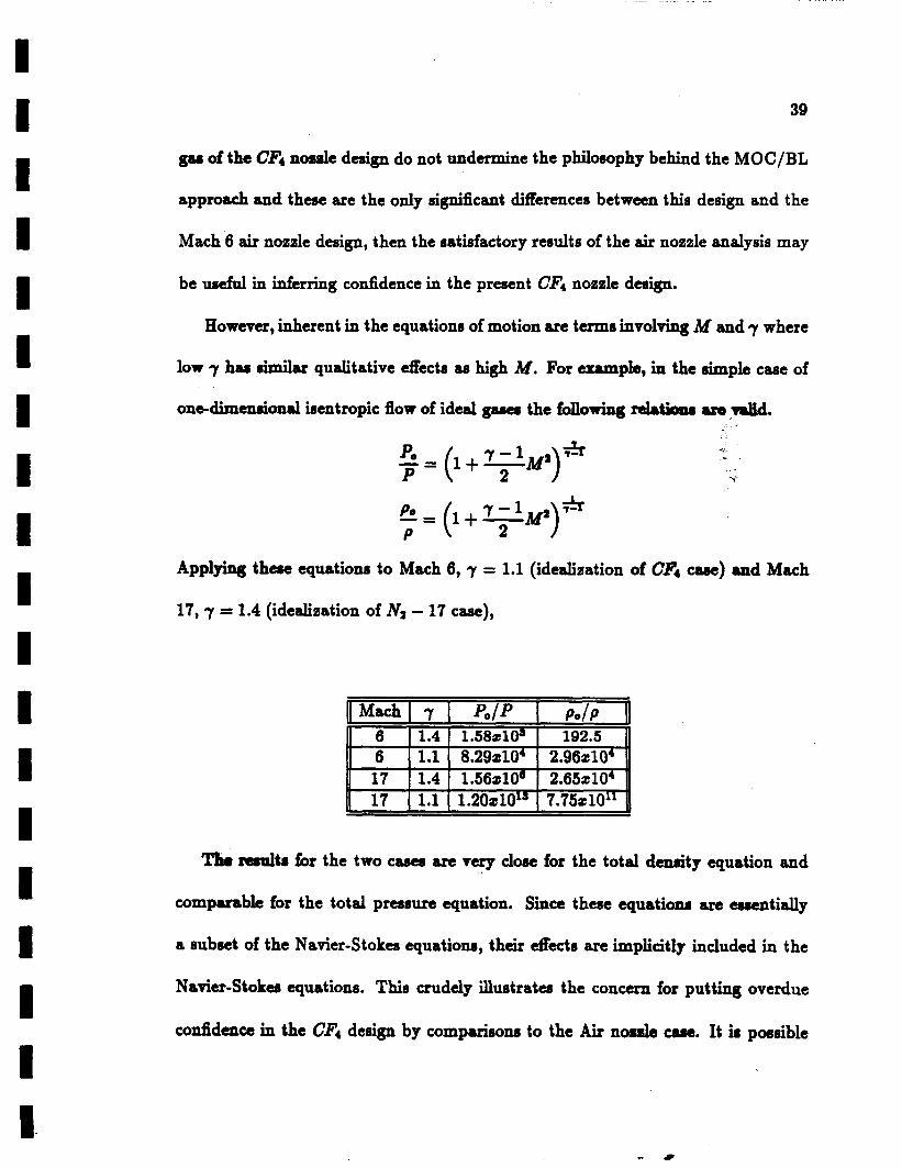
However, inherent in the equations of motion are tumrr involving M and 7 where

low 7 has similar qualitative effects as high M. For example, in the simple case of

one-dimdonad isentropic flow of i d 4 gams the f&wing datimu a m did.

Applying there equationa to Mach 6, 7 = 1.1 (idealisation of C.4 caoe) and Mach

17,7 = 1.4 (idealization of NZ - 17 case),

I I I n 17 11.4 I 1.56210'' I 2.65210' I

17 I 1.1 I 1.20~10'~ I 7.75~10"

"he d t a tor the two cases are very close for the total dearity equation and

comparable for the total prcsrure equation. Since these equations am essentially

a subact of the Navier-Stokes equations, their dects are implicitly included in the

Navier-Stoka equations. This crudely illustrates the concern for putting overdue

coddenct in the CF4 design by comparisons to the Air node case. It ir possible

1 I 1 I I I I I I I I I I 1 1 I I I I

40

that the apparent amplification of the compression wave in the analysis of the pre-

ceding nitrogen nozzles could take place in the C'4 nozzle only through a decreased

7 rather than an increased Mach number.

I 1 I I I I I I I I 1 I I 1 I I I I I

41

7 Conclusions 1. The Mach 6 air norale is designed to fit all design constraints. The Navier-

Stokes analysis of the design reveab a weak compression wave and predicts the

nozzle to expand slightly beyond design. Overall however, the Navier-Stokes

solution shows good quantitative agreement with the design conditions.

2. The Mach 13.5 nozzle for the Hypersonic Nitrogen Tunnel in dedQled to fit

all design constraints. The Navier-Stokes analysir shorn poor &ent with >*,

the design flow conditions. The nosale is predicted to be underexpanded and

has a series of oblique cornpression waves contaminating the flow.

3. Two Mach 17 nozzle contours are designed for the Hypersonic Nitrogen Tunnel

to fit all design constraints. The Navier-Stokes solutions show poor agreement

with the design flow conditions. Both contours are predicted to have oblique

compreesion waves. One contour expands to design conditions on the cen-

terline before the compression waves shock the core down and the.other is

predicted to be underexpanded.

4. The Mach 6 CF, n o d e for the Hypersonic CF, Tunnel is designed to fit

all design constraints. The Navier-Stokes analysis of the nosale contour is

unsuccessful because of numerical instabilities in the computer code. Because

the eflects of low 7 on nozzle flows are suspected to be similar to those of

42

high Mach number ( the Na - 13 and N2 - 17 cases), the flow in this nozzle

may be characterized by a compression wave from the idection point of such

strength as to shock down the nozzle.

5. The source of the compression waves seen in all Navier-Stokes solutions ema-

nating from near the inflection point of the nodes is not prcciaely determined,

If the apparent amplification of the downdream effectr of the waves with Mach

number can be attributed to a limitation in the current node design meth-

oda rather than a numerical limitation in the Navier-Stoksr andpia of high

sped internal flows, then the present state of MOC/BL node design is not

adequate to give reliable contoured noazle designs at higher Mach numbers.

6. If such a limitations exists then it appears to be in between Mach 8 and Mach

12. The current methods are shown here to work adequately for Mach 6 and

in an unpublished study for Mach 8. Problems have been recorded elsewhere

at Mach 12 and in this study at Mach 13.5 and Mach 17.

7. Further research is required in the area of high Mach number MOC/BL con-

toured wind tunnel nozzle design in order to determine whether the apparent

limitations of the current techniques are rooted in the design methods or were

caused by the Navier-Stokes analysi8.

1 1 I 1 I I I I 1 I I 1 I I 1 I 1 1 I

I I 1 I I 1 I I I I I I 1 I I I I I 1

43

8 Recommendations This project was originally conceived as a development project - specifically,

to develop hypersonic wind tunnels to meet the standard of high quality flow. Over

the course of the effort many areas within the nozzle design discipline have been

discovered where limitations in the current methods are apparent. Some serious

and baaic rcacarch is needed in this area. The following ir a partial liat u to where

the author feels this research should be concentrated.

1. Develop a Navier-Stokes solver specifically designed for internal flow problems,

particularly axisymmetric geometries. This code should have the following

characteristics:

0 adjustable CFL condition according to gradienta within the flow so that

entire nozzles can be loaded into a single run.

0 use of effective 7’s and compressibility factor, 2, so that equilibrium

effects and real gas virial effects can be easily included and updated

every 5 to 10 time steps.

0 use of finite volume scheme instead of finite difFerence scheme. The

author feels that the volumetric approach is a more sophisticated way to

approach the axisymmetric centerline problem.

44

0 remuch is needed to provide a reliable, accurate subsonic inflow bound-

ary condition or starting solution for these and other flows,

2. Perform extensive parametric studies using MOC/BL nozzle design and Navier-

Stokes analysis to gain basic understanding of how design parameters ef-

fect nosale flow and to get a better understanding of the limitations of the

MOC/BL approach.

3. If further research concludes that the current MOC/BL techniques become

inaccurate at some limiting Mach number, research rhould procad in devel-

oping an alternative design algorithm. A spacial mar- technique that can

be used in conjunction with the Parabobed Navier-Stokea equations should

be investigated.

I I I I 1 I 1 I I I I I I I I 1 I I I

I I

I I I

I I

45

\

46

References [l] Trimmer, L. L. and Voisinet, R. L., "The Optimum Hypersonic Wind Tunnel,"

AIAA Paper 86-0739-CP, March 1986.

[2] Clark et al., "Recent Work in Flow Evaluation and Techniquca of Operations for the Langley Hypersonic Nitrogen Facility," Fifth Hypervelocity Techniques Symposium, March 1967.

(31 Miller, C. G. and Smith, F. M., "Langley Hypersonic FacWer Complex - Description and Application," AIAA Paper 8&0741-CP, March 1986.

[41 Arhgton, J. P. et al., "Longitudinal Characteriatica of Several Codgustions at Hypemonk Mach Numbera in Conical and Contoured Nodes," NASA T N D-2489, September 1964.

[5] Midden, R. E. and Miller, C. G., "Description of the Laugley Hypemonic CF, Tunnel," NASA TP-2384, M u c h 1985.

[6] Thompaon, R. A. and Sutton K., "Computational Andyaia of the Langley Hypcmonic CF. Tunnel Nozzle and Preliminary Redesigh," NASA TM-89042, March 1987.

(71 J o h n , C. B. et al., "Real-Gaa Effects on Hypersonic Nossle Contours with

[8] Johnson, C. B. and Boney, L. R., "A Method for Calculating a Real-Gas Two- Dimensional Nozzle Contour Including the Effects of Gamma," NASA TM

a Method of Calculation," NASA TN D-1622, April 1963.

X-3243.

(91 Anderson, E. C. and Lewir C. H., "Laminar or Turbulent Boundary-Layer Flows of Perfect Gases or Reacting Gaa Mixtures in Chemical Equilibrium," NASA CR1893.

[lo] Zucrow, M. J. and Hofhan, J. D., Gas Dynamics, Volume 2: Multidi-

[ll] Kumar, A., "Numerical Analysis of the Scramjet Inlet Flow Using Two Dimen-

[12] Hunt, J. L. and Boney, L.R., "Thermodynamic and 'humport Properties of Ga~coua Tetraflouromethane in Chemical Equilibrium," NASA T N D-7181, 1973.

menaional Flow, John Why 8 SOM, Inc., 1977.

sional Navier-Stokes Equatiom," AIAA Paper 81-0185, January 1981.

PRECEDING PRGE BLANK NOT FILMED

I I I I I I I I I I I I I I 1 I I I I

I I I 1 I I I I I I I 1 I I 1 I I I

47

[13] White, Frank M., Viscow Fluid Flow, McGraw-Hill Book Company, New York, 1974.

[14] Baldwin, B.S. and Lomax, H., "Thin Layer Approimation and Algebraic

[15] Anderson, D. A., Tannehill, J.C, Pletcher R. H., Computational Fluid Me- chanics and Heat Transfer, Hemisphere Publishing Corporation, New York, 1984.

Model for Seperated Turbulent Flows," AIAA Paper 78-257, January, 1978.

Appendices

I I I 1 I I 1 I I I I I 1 I I I 1 I I

48

I I I I I I I I I I I I I I I I I I I.

49

A Method of Characteristics Applied to Nozzles

The equations governing axisymmetnc, irrotational, steady, supersonic flow-

fields, equations (A.l) and (A.2), are hyperbolic, quaei-linear partial differential

equations and can therefore be solved using the Method of Characteristics (MOC).

In a hyperbolic system, there exist charactdotic cum- (characteriath) dong

which the governing partial difierential equations CM be manipulated into ordi-

nary diflerential equations called eomputobilifp tqwtionr. Acrou churrckna tics,

flow propertica may have discontinuous derivatives while the property it& remains

continuous. For these equations,

(1 - ;) us - (5) ZLy + (1 - $) vu = -- V

Y

which are a composite of the continuity equation and Euler's equation (A.l) and

the itrotatiow2 condition eqn (A.2), the cornpatability equations are shown in [lo]

to be, ' sinptanpein6

sin(9 f p ) ($)& = f d 6 t a n p +

The equations are valid along the characteristic ha,

50

Equation6 (A.3) are readily expressed in finite difference form and can therefore be

easily integrated over a mesh of characteristic curves described by equations (A.3)

and (A.4).

Four equations are available relating the five variables 2,y, V, B and p, so one

additional relationship is needed. This is found by using the d a t i o n of the Mach

=de,

p = sin-' ($) , and a real-gaa relationship betwan M and V. The latter is achieved br t.bulating

M and V through an isentropic expansion including real-gar d k t r . In general, the

four equations are integrated in a marching scheme uing the modifitd Euler pre-

dictor/corrector method with an iterative algorithm on the corrector step. Details

of this procedure are found in [lo]. A direct marching technique ie used for the de-

sign and analysis procedures, meaning that the left and right running characteristic

waves (C+ and C, characteristics, respectively) make-up the computational grid.

A.l Design Procedure

The MOC design procedure used here is baaed primarily on that of reference

[8], which ia a modification of the work presented in [7]. Integration begins with

the design condition. That is, the starting solution is the 6nal characteristic DE

in Fig. 1.3. For this approach one must specify the solution along ABDE. The

maximum turning angle of a contoured nozzle occurs at point C of Fig. 1.3, the

I I I I 1 I I I I I I I I I I I I I I

I I I I I I I I I I I I 1 I I I I I I

51

inliedion point. The angle of the characteristic w d here, e,, must be specified.

A.l.l Radial Flow Region

Region I1 of Fig. 1.3 is called the radial flow region and is governed by the

characteristic radial flow equations, (A.6) and (A.7), which are the Prandtl-Meyer

expansion function and the radial velocity relationship.

and

(A.7)

Here 0, is the flow angle and is the Prandtl-Meyer expansion function h r radial

flow. For these equations, r is the distance &om the source shown on the centerline

upstream of point A in Fig. 1.3, and re is the sonic radius in source flow. These

equations are numerically integrated using an arbitrarily small velocity step AV

and the tabulated relation for M and V until the known design velocity is reached.

The integration of eq. (A.7) to V , fixes the location of point D. The relationship

between 2, V, 02 is retained and used aa the centerline solution on BD. Using the

and

e, = ef - ern along BC

52

equation (A.lO) is derived.

eIB = ern - 2ec. (A.lO)

41, can now be used in conjunction with the previously retained relationship be-

tween t+ and 5 to determine the location and flow solution at point B. The ten-

terline solution is now fixed on AB by assuming a M or V dbtribution. Using sonic

conditions at A and the known solution at B, one has the freedom to specify a first,

second or third order distribution. With the solution now Gxed along ABD, it is

left to determine the solution at the exit, the starting point of integration, line DE.

A.1.3 Uniform Flow Region

Region IV is the uniform flow region of a contoured node aince it is desired

to have constant properties and no flow angularity. Therefore, the solution along

DE is known to be the design conditions. However, it is still left to spacially locate

point E, which is k e d by the mass flux through the nozzle since all flow properties

on DE are known. The calculation of the limiting mass flux employs the stream

function concept and is reviewed in the following section.

A.l.3 Stream Function and Inviscid Wall Boundary

Integration along the characteristics for the design procedure begins at the cen-

terline where there are two points of known solution. A C+ characteristic through

a centerline point and a C- characteristic through a point on the starting charac-

teristic are used to simultaneously integrate equations (A.3) and (A.4) for the flow

I I I I I I I I I I I I I I I I I I I

c

I I 53

solution at another point on the second right running characteristic. The general

procedure is to calculate the stream function, $, along with the other flow variables, I at each point until it reaches the value limited by the mass flow. &irn is calculated

in the radial flow region at point C, the inflection point of the contour. Integration

of the axisymrnetric radial flow relation for $, eq.(A.11),

I

I I I I I I I I I I I I I I

where

gives the following result after evaluating a constant of integration.

. ( A . l l )

(A.12)

Again, equations (A.8) and (A.9) are used with the retained radial flows relationship

to determine and V at point C. The real-gas relationship between p and V is

obtained from tables. The equation for ?,b used while integrating the characteristic

mesh is

(A.13)

where a dm to the distance along the Mach wave and y is the perpendicular

distance from the x h a . When, during integration of eqs. (A.13), $l;,,, is reached,

integration stops, the wall point location is recorded and a new Mach line is started.

54

A.1.4 Iterative Procedure

For the present designs the exit radius is a design constraint. This means that

two nested iterative procedures will be needed to get a converged design. The outer

iteration k set up to converge on the design exit radius. The inner iteration is

designed to converge on the correct value of 6' at each 2 station for each contour

in the outer iteration.

An initial guess for 6' at the exit is necessary and the nondimenrionrl inviscid

contour t scaled so that its exit radiun in equal to the design radius minw the

g u e a d 6'. The boundary layer code (aee Appendix B) is used to F a t e 6'

for these coordinates and this is added to the scaled invbcid coordindsr to get

an initial guess for the corrected wall, y-. Now, each time the coordinates are

scaled or adjusted the curvilinear distance, 8 , of the nozzle contour is changed and

since 6' = 6'(8), the displacement thickness is ale0 changed. So, a second iterative

procedure is followed to find the correct value of 6' at each x-location. Here ymt is

adjusted at each x-location by

after mexy iteration on 6' until is lesa than a specified small e.

If the exit radius of the newly adjusted wall is not equal to the design radius,

then this wall is scaled to the design exit radius and the inner iteration loop is

repeated until they are equal.

I I I I I I I I I I 1 I I I I I I I I

I I 55

I I I I

A.3 Analysis Procedure

The present MOC analysis code is based on chapters 12 through 15 of [lo].

Integration of eqs (A.3) and (A.4) along the characteristics proceeds as in the design

case. The main differences between the design and analysis procedures are in the

starting solution and the techniques for dealing with the boundaries. Integration

begins near the throat on what is referred to as the initial value dution.

A.3.1 Wall Point

Sketch A.l illustrates the w d point situation. The presence of the solid bound-

ary clearly climinates the C, characterietic. However, the wall location L known

and the flow tangency relationshipe, 6 are known (the slope of the wall). So for the

three unknowne, M, p and V we have three equations, the cornpatability equation

for the C+ characteristic, the tabular real-gas isentropic expaneion of the gas and

the Mach wave relation.

I I I

56

1 9 I.

Loft-running durvtrinic c+

I t Knownintuiapoim

/ /

x

Sketch A.l Direct wall point solution by MOC.

p = sin-' (h) ' - dY = tane = - 11

dx U'

M = M ( V ) .

A.2.3 Centerline Point

A dmrlar situation arises at the axis (see sketch A.2). However for this case both

characteriatica exist. The flow properties at point 1 are merely reflected to point

2 exploiting the symmetry condition of the axisymmetric centerline. Furthermore,

cornpatability equations are simplified greatly since y or u are zero at the centerline

I I I I I I I I 1 I I I I I I I I I I

57

I I I I I I I 1 1 1 I I I I 1

so that only the C, characteristic is needed.

Ri@t-running charmoristic C-

Axis of wmwuny > X

2

Sketch A.2 Centerline point solution by MOC.

A.2.3 Iterative Procedure

To start the analysis iteration, an initial guess for 6' is needed. This is obtained

by generating a boundary layer using one-dimensional isentropic expansion to the

design Mach number as the edge conditione. The boundary layer correction is

subtracted Erom the actual nozzle wall to get a first guess for the characteristic

coordinates. The MOC analysis code is run on these coordinates. From the analysis

output, a second, hopefully better, estimate of 6' is generated. This is iterated until

the changes in 6' are small.

When and if a strong oblique shock wave forms in the MOC analysis solution,

then convergence may not be reached. The current status of the MOC/BL anal-

,-

58

ysis procedure is not generally sophisticated enough to account for strong shock-

wave/boundary layer interactions.

c

I I I I I I I I I I 1 I I I I I I I 1

I I I I I 1 I I 1 I I I I I 1 I 1 1 I

59

2 Numerical Solution of the Boundary Layer Equations

E. C. Anderson developed a computer program with the objective of generating

turbulent boundaq layer solutions for hypersonic flows, external and internal [9].

A brief overview of the techniques used is presented here.

The Crank-Nicohn semi-implicit finite Merence method i~ employed to inte-

grate the steady momentum, energy, species, and continuity tqurrtiOnr. The pro-

gram ir limited to gues in chemical equilibrium. By assuming a coxutcmt gar com-

position acrms the boundary layer, the effects of chemical reactioxu are included in

the heat transfer terms of the energy equation. In terms of non-dimensional vari-

ables these equations are, in axisymmetric form,

Continuity

Momentum

Energy

Continuity

Momentum

60

The above non-dimensional, turbulent boundary layer equations are transformed

using the Levy-Lees transformation (eqs. B.4 and B.5) to appear in the form of

equations (B.6), (B.7) and (B.8).

24Ft + V' + F = 0

2tFFt + VF, = @ - - Fa + (C(1+ .+)P)' ('a 1 Energy

where,

Since Crank-Nicolson technique is semi-implicit, the finite dif€erence represen-

tation of these equations contains independent variables at the station where the

solution is desired. This requires a matrix inversion, or an iterative procedure. An

1 I I I I 1 I I I I I I I 1 1 1 I I I

J

61

iterative procedure is used here. The coefficients of the independent variables are

evaluated using properties at the previous station. The finite difference equations

for energy and momentum are solved for the independent variables at the new sta-

tion. At each iteration the continuity equation is integrated using the trapezoidal

d e for the normal velocity, v. From the new properties, better estimates for the

coefficients are calculated and the procedure ie iterated until converged.

Once the solution hae converged at a particular station, eq (B.9) ir integrated

trapemidally from the wall to the point where pu/p,U, = 0.996.

I I I

follows.

I 1 I

, . ' (2.9)

The point in the boundary layer where this o c m is called the &placement thick-

ness and is used as the boundary layer correction to the MOC inviscid flow region.

The turbulence model is algebraic and is based on a two layer eddy viscosity

assumption. Hence, the Reynolds streas and turbulent heat transfer are defined as

C*&+ Prt = - &k

The total shear stress and heat transfer become,

(2.10)

(2.11)

(2.12)

62

(2.13)

The eddy viscosity is modeled assuming two layers. Both inner layer and outer

layer models for c+ are evaluated until

ri+ = e,. +

Below this point in the boundary layer e? ie d and above thia point e t ia used.

The outer layer is modeled by a aero equation mod4 developed by Clam (eq.

B.14).

(2.14)

Here,

parameter, and k2 is an empirical constant.

is the incompreseible dieplacement thickness, EW ie a coordinate stretching

The inner layer is based on Prandtl's mixing length theory and uses the Cebeci-

Smith aero equation turbulence model. The eddy viscosity for this layer is,

where,

kl = constant.

I I I I I I I I I I I I I I I I I I I

I I . I I I I I I I I I I I I I I I I I

63

3 Turbulence Modeling for Navier-Stokes Solutions

The turbulent Navier-Stokes equations are identical to the laminar equations

with the exception of additional terms in the turbulent expressions for heat transfer

(3.1) and the stress tensor (3.2).

( 3 4

However, these two terms introduce many additional unknowna to the problem

which can be defined only by the already unknown turbulent structure. These un-

knowns are dependant not only upon the physical properties of the particular gas,

but also upon local conditions such M velocity, geometry, surface roughness, and

previous spacial and temporal conditions [13]. Following the original idea of Boussi-

nesq (1877), one can model the e f i c t of turbulence - rather than model the actual

physics - and approach mathematical closure by considering the turbulent terms

ILI functionr of local geometry and flow properties. By defining the turbulent shear

(3.3) and turbulent heat transfer (3.4) in terms of effective turbulent coefficients of

viscosity, and thermal conductivity, h,

64

the assumption is that the turbulent terms behave similarly to their laminar (i.e. ,

physical) counterparts. Thus, in the stress and heat transfer equations of equation

set (M),

P = Pi + Pt

and

In thin research the turbulent conductivity is supplied through the turbulent Prandtl

number,

and ia considered to be constant at an empirical value of 0.9. The turbulent viscosity

is furnished by the Baldwin-Lomax two layer eddy viscosity model [14].

3.1 Baldwin-Lomax Turbulence Model

The Baldwin-Lomax two layer eddy viscosity model was developed to address

the problem of including turbulent effects in Navier-Stokes simulations of separated

flows where the boundary layer thickness is not generally known. Baldwin and

Lorn= (141 defined the eddy viscosity on an inner and outer layer by

(3.5)

where yeor- ia the shortest normal distance from the wall at which the inner and

outer COefEcients are equal.

I I I I I I I I I I I I I I I I I I I

65

I I I I I I I

I I I I

The Prandtl-Van Driest formulation is used for the inner region.

(pt)innat = PI' IW I

where

I = ky [l - exp (-y+/A+)]

IwI is the magnitude of the vorticity

and

The formulation for the outer region is

(3.6)

(3.7)

(3.10)

where K is the Clauser constant Ccp is an additional constant and

(3.11)

min

The mlrimrrm point of the function (3.12) and the point at which it occurs define

(3.12)

Fala is the KlebanoE intermittency factor expressed as

(3.13)

I I

66

and the quantity udf is the difference between the maximum and minimum total

velocities, which for no slip boundary conditions is the maximum total velocity in

the profile. The following constants are used in the turbulent viscosity calculations.

A+ = 26

Ccp = 1.6

C ~ l d = 0.3

C,, = 0.25

A = 0.4

K = 0.0168

I I I I I I I I 1 I I I I I I I I I I

67

7 Working Exit Exit Total Po To - Nozzle Gas Dim. Mach Length psia O R

NZ - 17 Nitrogen 20 in. 17 - N2 - 13 Nitronen 20in. 13.5 -

4000 3400 4000 3000

Tables

I

I I

K - i

1600 1260 He20 Helium 21in. 20 124in. 1500 600

Air Air - 7.2in. 5.95 - 76h. 4!5 1260

I (7 .4 CFI 20 in. 5.95 -

I I I I

' & ' 4.025724 x 10" Ba -1.149705~ 10' a -1.059139 x lo4

I I I I

CS -3.162000 x " K 1.758236 -

- c4 5.15767~ lo-' 4 -1.59381 x -

Table 2. Constants for CF, Thermodynamic Equatiom nR I 94.47002 11 b I 0.0015

"

h

,a -1.0727 x 4 2.64172 x L

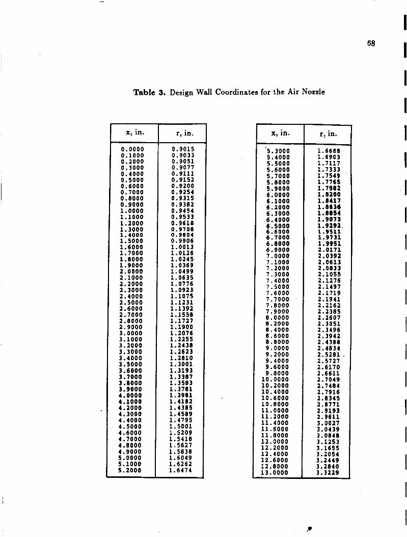
Table 3. Design Wall Coordinates for the Air Nozzle

x, in. ~ ~~

0.0000 0.1000 0.2000 0.3000 0.4000 0.5000 0.6000 0.7000 0.8000 0 .goo0 1.0000 1.1000 1.2000 1.3000 1.4000 1. 5000 1.6000 1.7000 1.8000 1.9000 2.0000 2.1000 2.2000 2.3000 2.4000 2. 5000 2.6000 2.1000 2. 8000 2.9000 3.0000 3.1000 3.2000 3.3000 3.4000 3. 5000 3.6000 3.1000 3.8000 3.9000 4.0000 4.1000 4.2000 4.3000 4.4000 4. 5000 4.6000 4 .lo00 4.8000 4.9000 5.0000 5.1000 5.2000

r, in.

0.9015 0.9033 0.9051 0.9077 0.9111 0.9152 0.9200 0.9254 0.9315 0.9382 0.9454 0.9533 0.9618 0.9708 0.9804 0.9906 1.0013 1.0126 1.0245 1.0369 1.0499 1.0635 1.0116 1.0923 1.1015 1.1231 1.1392 1.1558 1.1127 1.1900 1.2016 1.2255 1.2438 1.2623 1.2810 1.3001 1.3193 1.3387 1.3583 1.3181 1.3981 1.4182 1.4385 1.4589 1.4195 1. 5001 1.5209 1.5418 1.5621 1.5838 1.6049 1.6262 1.6414

x, in. r, in. i 1 -

5.3000 i 1.6688 5.4000 5. 5000 5.6000 5.7000 5.8000 5.9000 6.0000 6.1000 6.2000 6.3000 6.4000 6.5000 6.6000 6.1000 6.8000 6.9000 7.0000 7.1000 7.2000 7.3000 7.4000 7.5000 7.6000 7.7000 7.8000 7.9000 8.0000 8.2000 8.4000 8.6000 8.8000 9.0000 9.2000 9.4000 9.6000 9. 8000

10.0000 10.2000 10.4000 10.6000 10.8000 11.0000 11.2000 11.4000 11.6000 11.8000 12.0000 12.2000 12.4000 12.6000 12.8000 13.0000

1.6903 1.1117 1.1333 1.1549 ’

1.1765 1.7982 1.8200 1.8417 1.8636 1.8854 1.9073 1.9292. 1.9511 1.9731 1.9951 2.0171 2.0392 2.0613 2.0833 2.1055 2.1216 2.1491 2.1119 2.1941 2.2162 2.2385 2.2601 2.3051 2.3496 2.3942 2.4388 2.4834 2.5281 . 2.5127 2.6170 2.6611 2.7049 2.1484 2.7916 2.8345 2.8711 2.9193 2.9611 3.0027 3.0439 3.0848 3.1253 3.1655 3.2054 3.2449 3.2840 3.3229

I 68 I

I I I I I I I I I I I I I I I I I

I I I I 1 I I I I I I 1 I I I . I I I I

I

r, in. ~ ~~

x, in.

28.0000 28. 5000 29.0000 29.5000 30.0000 30.5000 31.0000 31.5000 32.0000 32.5000 33.0000

13.2000 13.4000 13.6000 13.8000 14.0000 14.2000 14.4000 14.6000 14.8000 15.0000 15.2000 15.4000 15.6000 15.8000 16.0000 16.2000 16.4000 16.6000 16.8000 17.0000 11.2000 17.4000 17.6000 17.8000 18. 0000 18. 2000 18.4000 18.6000 18,8000 19.0000 19.2000 19.4000 19.6000 19.8000 20.0000 20.2000 20.4000 20.6000 20.8000 21.0000 21.2000 21.4000 21.6000 21.8000 22.0000 22.2000 22.4000 22.6000 22.8000 23.0000 23. 5000 24.0000 24.5000 25.0000 25. 5000 26.0000 16.5000 L7.0000 L7.5000

, 33.5000 34.0000 34.5000 35.0000 35.5000 36.0000 36.5000 37.0000 37.5000 38.0000 38. SO00 39.0000 39.5000 40.0000 40.5000 41.0000 41.5000 42.0000 42.5000 43.0000 43.5000 44.0000 4 4 . 5000 45.0000 45.5000 46.0000 46. 5000 47.0000 47. SO00 48.0000 48. 5000 49.0000 49. 5000 50.0000 51.0000 52.0000 53.0000 54.0000 55 .0000 56.0000 57.0000 58.0000 59.0000 60.0000 61.0000 62.0000 63.0000 64.0000

69 Table 3. (continued)

3.3614 3.3996 3.4375 3.4750 3.5122 3.5491 3.5857 3.6219 3.6579 3.6935 3.7288 3.7638 3.7985 3 .a330 3.8671 3.9009 3.9345 3.9677 4.0007 4.0333 4.0657 4.0978 4.1297 4.1612 4.1925 4.2235 4.2543 4.2847 4.3150 4.3449 4.3746 4.4040 4.4332 4.4622 4.4909 4.5193 4 .5475 4.5755 4.6032 4.6307 4.6580 4.6850 4.7118 4.7383 4.7646 4.7907 4.8166 4.8422 4.8677 4.8929 4.9549 5.0157 5.0752 5 . 1 3 3 4 5.1904 5.2461 5.3007 5.3541 5.4063

[ X, in. r, in.

5 . 4 5 7 4 5.5075 5.5564 5.6043 5.6511 5.6970 5.7418 5.7857 5.8285 5.8705 5.9115 5.9516 5.9908 6.0292 6.0666 6.1033 6.1392. 6.1740 6.2002 6.2416 6.2742 6.3060 6.3371 6.3674 6.3971 6.4260 6.4542 6.4817 6.5085 6.5347 6.5602 6.5851 6.6094 6.6330 6.6560 6.6784 6.7002 6.7215 6.7421 6.7622 6.7818 6.8008 6.8193 6.8372 6.8547 6.8880 6.9194 6.9489 6.9766 7.0026 7.0268 7.0494 7.0705 7.0901 7.1082 7.1249 7.1403 7.1544 7.1672

c

Table 3. (continued)

71.0000 72.0000 73.0000 74.0000 75.0000 76.0000

I x, in. r, in.

7.2296 7.2374 7.2451 7.2528 7.2605 7.2681

-~~

65.0000 66.0000 67.0000 68.0000 69.0000 70.0000

7.1789 7.1891 7.1976 7.2057 7.2137 7.2217

I I I x, in. I r, in.

I 70 I

I I I I I I I I I I I I 1 I I I I

I I I I I I I I I I I I I I I I I I 1.

.

71

x, in.

0.0000 0.1000 0.2000 0.3000 0.4000 0. 5000 0.6000 0.7000 0.8000 0.9000 1.0000 1.1000 1.2000 1.3000 1.4000 1. 5000 1.6000 1.7000 1 .a000 1.9000 2.0000 2.1000 2.2000 2.3000 2.4000 2.5000 2.6000 2.7000 2.8000 2.9000 3.0000 3.1000 3.2000 3.3000 3.4000 3.5000 3.6000 3.7000 3.8000 3.9000 4.0000 4.1000 4.2000 4.3000 4.4000 4 . 5000 4.6000 4.7000 4.8000 4.9000 5.0000 5.1000 5.2000

Table 4. Design Wall Coordinates for the Nz - 13.5 Nozzle

r, in.

0.1194 0.1202 0.1224 0.1256 0.1298 0.1351 0.1413 0.1484 0.1566 0.1657, 0.1757 0.1869 0.1990 0.2122 0.2266 0.2421 0.2S87 0.2762 0.2946 0.3135 0.3331 0.3531 0.3735 0.3943 0.4153 0.4365 0.4579 0.4796 0.5013 0.5232 0.5452 0.5673 0.5895 0.6117 0.6341 0.6564 0.6789 0.7014 0.7239 0.7465 0.7692 0.7918 0.8146 0.8373 0.8601 0.8829 0.9058 0.9287 0.9516 0.9745 0.9974 1.0204 1 . 0 4 3 t

x, in.

5.3000 5.4000 5. 5000 5.6000 5.7000 5.8000 5.9000 6.0000 6.1000 6.2000 6.3000

6.5000 6.6000 6.7000 6.8000 6.9000 7.0000 7.1000 7.2000 7.3000 7.4000 7.5000 7.6000 7.7000 7.8000 7.9000 8.0000 8.1000 8.2000 8.3000 8.4000 8.5000 8.6000 8.7000 8.8000 8.9000 9.0000 9.1000 9.2000 9.3000 9.4000 9.5000 9.6000 9.7000 9.8000 9.9000

PO. 0000 0.1000 0.2000 0.3000 0.4000 0.5000

6 4000

r, in.

1.0661 1.0888 1 .1114 1.1339 1.1563 1 . 1 7 8 ~ 1.2007 1.222& 1.2447

-

KJ 1.3315 1. 3S2S6 1 .3742 1.39S4 1.4165 1.4375 1.4584 1.4792 1.4999 1.5205 1.5410 1.5614 1.5817 1.6019 1.6220 1.6420 1.6619 1.6818 1.7015 1.7211 1.7406 1.7601 1.7794 1.7987 1.8179 1.8370 1.8560 1 .a749 1.8937 1.9125 1.9311 1.9497 1.9682 1.9867 2.0050 2.0233 2.0414 2.0595 2.0776 2.0955 2.1134

Table

x, in.

21.5000 21.8000 22.1000 22.4000 22.7000 23.0000 23.3000 23.6000 23.9000 24.2000 24.5000 24.8000 25.1000 25.4000 25.7000 26.0000 26.3000 26.6000 26.9000 27.2000 27. 5000 27.8000 28.1000 28.4000 28.7000 29.0000 29.3000 29.6000 *

29.9000 30.2000 30. 5000 30.8000 31.1000 31.4000 31.7000 32.0000 32.3000 32.6000 32.9000 33.2000 33.5000 33.8000 34.1000 34.4000 34.7000 35.0000 35.3000 35.6000 35.9000 36.2000 36. 5000 36.8000 37.1000 37.4000 37.7000 38.0000 38.3000 38.6000 38.9000

4. (continu

r, in.

3.1423 3.7796 3.8166 3.8533 3.8898 3.9259 3.9618 3.9974 4.0327 4.0678 4 .lo26 4.1371 4.1714 4.2094 4.2392 4.2721 4.3061 4.3391 4.3720 4.4046 4.4369 1.4691 4 . SO10 4.5327 4.5642 4.5954 4.6265 4.6574 4.6880 4.7184 4.7487 4.7787 4.8085 4.8382 4.8676 4.8969 4.9259 4. 9548 4. 9835 5.0120 5.0403 5.0685 5.0964 5.1242 5.1519 5.1793 5.2066 5.2337 5.2607 5.2815 5.3141 5.3405 5.3668 5.3930 5.4189 5.4448 5.4704 5.4960 5.5213

I r, in. I x, in.

10.6000 10.7000 10.8000 10.9000 11.0000 11.1000 11.2000 11.3000 11.4000 11 5000 11.6000 11.7000 11.8000 11.9000 12.0000 12.2000 12.4000 12.6000 12.8000 13.QQQQ 13.2000 13.4000 13.6000 13 .a000 14.0000 14.2000 14.4000 14.6000 14.8000 15.0000 15.2000 15.4000 15.6000 15.8000 16.0000 16.2000 16.4000 16.6000 16.8000 17.0000 17.2000 17.4000 17.6000 17.8000 18.0000 18.2000 18.4000 18.6000 18.8000 19.0000 19.2000 19.4000 19.6000 19.8000 20.0000 20.3000 20.6000 20.9000 21.2000

2.1312 2.1489 2.1666 2.1841 2.2017 2.2191 2.2365 2.2538 2.2710 2.2882 2.3052 2.3223 2.3392 2.3561 2.3730 2.4064 2.4397 2.4727 2. SO54 2.5379 2.5702 2.6023 2.6341 2.6657 2.6971 2.7282 2.7592 2.7899 2.8204 2.8508 2.8809 2.9109 2.9406 2.9702 2.9996 3.0287 3.0577 3.0866 3.1152 3.1437 3.1720 3.2001 3.2281 3.2559 3.2835 3.3110 3.3383 3.3654 3.3925 3.4193 3.4460 3.4725 3.4989 3.5251 3.5512 3.5901 3.6286 3.6668 3.7047

72

I 1 1 i 1 1 1 1 1 1 I I I I I I I I I

I I I 1 I 1 I 1 1 I I I 1 I I I 1 I 1

.

x, in.

39.5000 39.8000 40.1000 40.4000 40.7000 41.0000 41.3000 41.6000 41.9000 42.2000 42. 5000 42.8000 43.1000 43.4000 43.7000 44.0000 44.3000 44.6000 44.9000 45.2000 45.5000 45.8000 46.1000 46.4000 46.7000 47.0000 47.3000 47.6000 47.9000 48.2000 48. 5000 48.8000 49.1000 49.4000 49.7000 SO .oooo 50 .so00 51 .oooo 51. so00 52 . O O O O 52. 5000 S3 .OOOO 53 5000 54 .OOOO 54. 5000 55 .OOOO 55. 5000 56.0000 56.5000 57.0000 57.5000 50.0000 58. 5000 59.0000 59. 5000 60.0000 60. SO00 61.0000

73

Table 4. (continued)

r, in.

5.5465 5.5716 5.5965 5.6213 5.6459 5,6704 5.6947 5.7189 5.7430 5.7669 S. 7907 5.8144 5.8379 5.8613 5.8845 5.9076 5,9306 5.9535 5.9762 5.9988 6.0212 6.0436 6.0658 6.0879 6.1099 6.1317 6.1535 6.1751 6.1966 6.2180 6.2392 6.2604 6.2814 6.3023 6.3231 6.3438 6.3644 6.3984 6.4321 6.4655 6.4987 6.5315 6.5641 6.5963 6.6283 6.6600 6.6914 6.7225 6.7533 6.7839 6.8143 6.8443

6.9036 6.9329 6.9619 6.9907 7.0192 7.0475

6.8741

x, in.

61.5000 62.0000 63.0000 64.0000 65.0000 66.0000 67.0000 68.0000 69.0000 70.0000 71.0000 72.0000 73.0000 74.0000 75.0000 76.0000 77.0000 78.0000 79.0000 80.0000 81.0000 82.0000 83.0000 84.0000 85.0000 86.0000 87.0000 88.0000 89.0000 90.0000 91.0000 92.0000 93.0000 94.0000 95.0000 96.0000 97 .QOQO 98.0000 99.0000

. o o . 0000

. 01 .0000

.02.0000

.03.0000

.04.0000 .os. 0000

.06.0000

.07.0000 08.0000 09.0000 10.0000 11.0000 12.0000 13.0000 14.0000 15.0000 16.0000 l?. 0000 17.5410

~

r, in.

7.0755 7.1032 7.1581 7.2119 7.2649 7.3169 7.3681 7.4183 7.4677 7.5163 7 -5640 . 7.6108 7: 6569 7.7021 7.7465 7.7902 7.8330 7.8752 7.9165 7.9571 7.9970 8.0362 8.0747 8.1124 8.1495 8.1858 8.2215 8.2565 8.2908 8.3245 8.3575 8.3899 8.4216 8.4526 8.4830 8.5128 8 .5419 8.5704 8.5983 8.6256 8.6523 8.6783 0.7037 8.7286 8.7528 8.7764 8.7993 8.8217 8 .a435 8.8646 8.8850 8.9049 8.9240 8.9424 8.9601 8.9768 8.9924 9.0000

Table 5. Design Wall Coordinates for the N2 - 17 Nozzle

.

x, in.

0.0000 0.0018 0.0066 0.0135 0.0235 0.0379 0.0585 0.0883 0.1311 0.1928 0.2617 0.4096 0.5934. 0.7934 . 0.9934 1.1934 1.3934 1.5934 1.1934 1.9934 2.1934 2.3934 2.5934 2.7934 2.9934 3.1934 3.3934 3.5934 3.7934 3.9934 4.1934 4.3934 4.5934 4.7934 4.9934 5.1934 5.3934 5.5934 s.7934 5.9934 6.1934 6.3934 6.5934 6.7934 6.9934 7.1934 7.3934 7.5934 7.7934 7.9934 8.2134 8.5302

r, in.

0.0607 0.0607 0.0607 0.0607 0.0607 0.0608 0.0608 0.0609 0.0610 0.0611 0.0613 0.0615 0.0620 0.0629 0.0646 0.0673 0.0718 0.0783 0.0866 0.0989 0.1154 0.1371 0.1666 0.2031 0.2429 0.2853 0.3295 0.3745 0.4208 0.4666 0.5133 0.5603 0.6077 0.6552 0.7028 0.7501 0.7969 0.8429 0.8883 0.9331 0.9773 1.0211 1.0643 1.1070 1.1493 1.1912 1.2329 1.2741 1.3145 1.3544 1.3978 1.4592

x, in.

8.9302 9.3302 9.7302

10.1302 10.5302 10.9302 11.3302 11.7302 12.1302 12.5302 12.9302 13.3302 13.7302 14.1302 14.5302 14.9302 15.3302 15.7302 16.1302 16.5302 16.9302 17.3302 17.7302 18.1302 18.5302 18.9302 19.3302 19.7302 20.1302 20.6582 21.2582 21.8582 22.4582 23.0582 23.6582 24.2582 24.8582 25.4582 26.0582 26.6582 27.2582 27.8582 28.4582 29.0582 29.6582 30.2582 30.8582 31.4582 32.0582 32.. 6582 33.2582 33.8582

r, in.

1.5355 1.6102 1.6836 1.7555 1.8266 1.0960 1 . 9 6 4 s

2.0983 2. o3it 2.163% 2.22.a 2.2924 2.3b47 2.4160

2.5407 2.6006 2.6599 2.7169 2.7773 2.8346 2.8912 2.9473 3.0027 3.0576 3.1118 3.1655 3.2188 3.2715 3.3403 3.4175 3.4936 3.5686 3.6426 3.7155 3.7874 3 .a585 3.9286 3.9980 4.0665 4 . 1 3 4 1 4.2010 4.2671 4.3325 4.3971 4.4611 4.5243 4.5.868 4.6488 4.7099 4.7706 4.8307

2 4791

1 74 1

1 i 1 i 1 1 1 1 111 1 1 1 1 1 1 1 1

I I I I I I I I I I I I I I I I I I I

.

x, in.

34 .4582 35 .0582 35 .6582 36 .2582 36 .8582 37 .4582 38 .0582 38 .6582 39 .2582 39 .8582 40 .4582 41 .0582 41 .6582 42 .2582 42 .8582 43 .4582 4 4 . 0 5 8 2 44 .6582 45 .2582 45 .8582 46 .4582

4 7 . 6 5 8 2 4 8 . 2 5 8 2 4 8 . 8 5 8 2 49 .4582 50 .OS82 50 .8182 51 .6182 52 .4182 53 .2182 54 .0182 54 .e182 5 5 . 6 1 8 2 5 6 . 4 1 8 2 57 .2182 56.0182 58 .a182 59 .6182 6 0 . 4 1 8 2 6 1 . 2 1 8 2 6 2 . 0 1 8 2

6 3 . 6 1 8 2 6 4 . 4 1 8 2 6 5 . 2 1 8 2 66 .0182 6 6 . e l 8 2 67 .6182 6 8 . 4 1 8 2 6 9 . 2 1 8 2 70 .0182 70 . e 1 8 2 7 1 . 6 1 8 2 72 .4182 1 3 . 2 1 8 2 7 4 . 0 1 8 2 74 .a182

47 .0502

6 a . 8 i t n

75 Table 5. (continued)

r, in. ~~

4 .8900 4 .9488 5 . 0 0 6 9 5 .0646 5 .1217 5 . 1 7 8 1 5 . 2 3 4 1 5 . 2 8 9 5 5 .3444 5 .3987 5.4526 5 . 5 0 5 9 5 .5586 5 . 6 1 0 8 5 ,6626 5.7141 5 .7649 5.8152 5 .8650 5 .9144 5 .9633 6 .0120 6 . 0 5 9 9 6 . 1 0 7 6 6 . 1 5 5 6 6 .2026 6 . 2 4 9 5 6 .3080 6 . 3 6 8 9 6 . 4 2 9 2 6 . 4 8 9 0 6 .5480 6 . 6 0 6 9 6 . 6 6 4 1 6 . 7 2 1 0 6 .7775 6 . 8 3 3 1 6 .8884 6 .9430 6 . 9 9 6 9 7 .0504 7 . 1 0 3 2 7 .1556 7 . 2 0 7 2 7 . 2 5 8 4 7 . 3 0 9 0 7 . 3 5 9 1 7 .4086 7 .4576 7 . SO61 7 . 5 5 4 1 7 . 6 0 1 6 7 . 6 4 8 6 7 . 6 9 5 2 7 . 7 4 1 3 7 . 7 8 6 7 7 . 8 3 1 8 7 . 8 7 5 6

x, in.

7 5 . 6 1 8 2 7 6 . 4 1 8 2 77 .2182 7 8 . 0 1 8 2 78 .8182 7 9 . 6 1 8 2 8 0 . 4 1 8 2 8 1 . 2 1 8 2 8 2 . 0 1 8 2 8 2 . 8 1 8 2 8 3 . 6 1 8 2 8 4 . 4 1 8 2 8 5 . 2 1 8 2 8 6 . 0 1 8 2 8 6 . 8 1 8 2 8 7 . 6 1 8 2 8 8 . 4 1 8 2 8 9 . 2 1 8 2 9 0 . 0 1 8 2 9 0 . 8 1 8 2 9 1 . 6 1 8 2 9 2 . 4 1 8 2 9 3 . 2 1 8 2 9 4 . 0 1 8 2 9 4 . 8 1 8 2 9 5 . 6 1 8 2 9 6 . 4 1 8 2 9 7 . 2 1 8 2 9 8 . 0 1 8 2 9 8 . 8 1 8 2 9 9 . 6 1 8 2

L O O . 4180 101 .2180 102 .0180 102.8180 103 .6180 104.4180 105.2180 106.0180 106.8180 107.6180 108.4180 109.2180 110.0180 110.8180 111.6180 112.4180 113.2180 114.0180 114.8180 115.6180 116.4180 117.2380 118.0180 .18 .a180 . 1 9 . 6 1 8 0 . 2 0 . 4 1 8 0 - 2 1 . 2 1 8 0

r, in.

7 .9191 7 .9622 8 . 0 0 5 0 8 . 0 4 7 4 8 .0894 8 . 1 3 1 1 8 .1724 8 .2134 8 .2540 8 .2942 8 .3341 8 .3736 8.4128 8.451s 8.49eQ 8.521% 8 . 5 6 5 8

8 . 6 7 6 8 8 . 7 1 3 1 8 . 7 4 9 0 8.7846. 8 . 8 1 9 8 8 . 8 5 4 8 8 . 8 8 9 1 8 . 9 2 3 3 8 . 9 5 7 0 8 . 9 9 0 4 9 . 0 2 3 5 9 . 0 5 6 2 9 . 0 8 8 5 9 . 1 2 0 5 9 . 1 5 2 1 9 . 1 8 3 3 9 . 2 1 4 2 9 . 2 4 4 7 9 . 2 7 4 9 9 . 3 0 4 7 9 . 3 3 4 2 9 . 3 6 3 3 9 . 3 9 2 0 9 . 4 2 0 4 9 .4484 9 . 4 7 6 0 9 .5033 9 . 5 3 0 3 9 . 5 5 6 8 9 . 5 8 3 1 9 .6089 9 .6344 9 . 6 5 9 5 9 .6843 9 . 7 0 8 7 9 . 7 3 2 8 9 . 7 5 6 5 9 . 7 7 9 9 9 . 8 0 2 8

8 . 8.6402 6031

Table 5. (continued)

x, in.

122.0180 122.8180 123.6180 124.4180 125.2180

r, in.

9.0254 9.8477 9.8696 9.8912 9.9123

x, in. r, in.

126.0ldO 9.9332 126.8180 9.9536 127.6180 9.9737 128.4180 9.9935 128.9060 10.0053

mblc 8. Design Wall Coordinates for the CF, N o d e

x, in.

0.0000 0.1000 0.2000 0.3000 0.4000 0. 5000 0.6000 0.7000 0 .a000 0.9000 1.0000 1.1000

.1.2000 1.3000 1 . 4000 1.5000 1.6000 1.7000 1.8000 1.9000 2.0000 2.1000 2.2000 2.3000 2.4000 2.5000

r, in.

0.2580 0.2581 0.2583. 0.2587 0.2592 0.2599 0.2607 0.2615 0.2625 0.2636 0.2649 0.2662 0.2677 0.2693 0.2709 0.2727 0.2746 0.2767 0.2788 0.2810 0.2833 0.2857 0.2882 0.2908 0.2935 0.2964

x, in.

2.6000 2.7000 2.8000 2.9000 3.0000 3.1000 3.2000 3.3000 3.4000 3.5000 3.6000 3.7000 3.8000 3.9000 4.0000 4.1000 4.2000 4.3000 4.4000 4.5000 4.6000 4.7000 4.8000 4.9000 5.0000 5.1000

r, in.

0.2993 0.3024 0.3055 0.3089 0.3123 0.3159 0.3196 0.3235 0.3275 0.3317 0.3360 0.3406 0.3453 0.3502 0.3551 0.3603 0.3656 0.3710 0.3767 0.3825 0.3885 0.3947 0.4011 0.4077 0.4145 0.4216

76

I 1 1 i 1 1 1 1 1 1 1 1 1 1 1 1 1 1 1

I I I I I I I I I I I I I I I I 1 I I

~~

x, in.

5.2000 5.3000 5.4000 5 . 5000 5.6000 5.7000 5.8000 5.9000 6.0000 6.1000 6.2000 6.3000 6.4000 6 . 5000 6.6000 6.7000 6.8000 6.9000 7.0000 7.1000 7.2000 7.3000 7.4000 7.5000 7.6000 7.7000 7.8000 7.9000 8.0000 8.1000 8.2000 8.3000 8.4000 8. 5000 8.6000 8.7000 8.8000 8.9000 9.0000 9,1000 9.2000 9.3000 9.4000 9. 5000 9.6000 9.7000 9 .a000 9.9000

10.0000 10.2000 10.4000 10.6000 10.8000 11.0000 11.2000 11.4000 11.6000 11.8000

77

Table 6. (continued)

r, in.

0.4288 0.4362 0.4439 0.4519 0.4600 0.4604 0.4771 0.4861 0.4953 0.5048 0.5146 0.5247 0.5352 0.5459 0.5570 0.5685 0.5803 0.5925 0.6051 0.6181 0.6316 0.6455 0.6599 0.6749 0.6903 0.7063 0.7228 0.7398 0.7573 0.7752 0.7936 0.8124 0.8316 0.8511 0.8710 0.8913 0.9119 0.9321 0.9539 0.9753 0.9970 1.0189 1.0411 1.0635 1.0861 1.1088 1.1318 1.1549 1.1782 1.2252 1.2727 1.3208 1.3693 1.4181 1.4613 1.5168 1.5668 1.6168

x, in.

12.0000 12.2000 12.4000 12.6000 12.8000 13.0000 13.2000 13.4000 13.6000 13.8000 14.0000 14.2000 14.4000 14.6000 14.8000 15.0000 15.2000 15.4000 15.6000 15.8000 16.0000 16.2000 16.4000 16.6000 16.8000 17.0000 17.2000 17.4000 17.6000 17.8000 18.0000 18.2000 18.4000 18.6000 18.8000 19.0QQO 19.2000 19.4QOO 19.6000 19.8000 20.0000 20.3000 20.6000 20.9000 21.2000 21. 5000 21.8000 22.1000 22.4000 22.7000 23.0000 23.3000 23.6000 23.9000 24.2000 24.5000 24.8000 25.1000

r, in.

1.6670 1.7173 1.7679 I. 8186 1 .e694 1.9205 1.9716 2.0229 2.0743 2.1258 2.1774 2.2290 2.2807 2.3324 2.3842 2.4360 2.4877 2.5394 2.5912 2.6431 2.6950 2.7469 2.7980 2.8506 2.9022 2.9535 3.0046 3.0554 3.1060 3.1563 3.2063 3.2561 3.3056 3.3548 3.4037 3 .4522 3.5006 3.5486 3.5963 3.6437 3.6909 3.7610 3 A 3 0 5 3.8993 3.9675 4.0350 4.1019 4.1682 4.2338 4.2988 4.3631 4.4269 4.4900 4.5526 4.6144 4.6757 4.7365 4.7966

x, in.

25.4000 25.7000 26.0000 26.3000 26.6000 26.9000 27.2000 27.4999 27.7999 28.0999 28.3999 28.6999 28.8999 29.1999 29.4999 29.7999 29.9999 30.4999 30.9999 31.4999 31.9999 32.4999 32.9999 33.4999 33.9999 34.4999 34.9999 35.4999 35.9999 36.4999 36.9999 37.4999 37.9999 38.4999 38.9999 39.5000 40.0000 40.5000 41.0000 41.5000 42.0000 42. 5000 43.0000 43.5000 44 .OOOO 44.5000 45.0000 45.5000 46.0000 46. SO04 47.0004 47. 5004

Table 6. (continued)

r, in.

4.8561 4.9152 4.9735 5.0314 5.0886 5.1453 5.2015 5.2572 5.3123 5.3668 5.4208 5.4743 5.5097 5.5623 5.6145 5.6661 5.7002 5.7846 S -8677 5.9494 6.0298 6.1091 6.1870 6.2637 6.3393 6.4136 6.4868 6.5588 6.6297 6.6994 6.7679 6.8354 6.9017 6.9670 7.0313 7.0945 7.1567 7.2178 7.2780 7.3372 7.3954 7.4527 7.5091 7.5645 7.6190 7.6726 7.7253 7.7772 7.8282 7.8783 7.9276 7.9761

x, in.

48.0004 48.5004 49.0004 49.5004 S O . 0004 5 1 . O O O ? 52.0004 53.0004 54 . O O M 55.0004 56.0008 57.0008 58.0008 59.0006 60.0008 61.0008 62.0008 63.0008 64.0012 65.0012 66.0012 67.0012 68.0012 69.0012 70.0012 71.0012 72.0012 73.0016 74.0016 75.0016 76.0016 77.0016 78.0016 79.0016 80.0016 81.0016 82.0016 83.0020 84.0020 85.0020 86.0020 87.0020 88.0020 89.0020 90.0020 91.0024 92.0024 93.0024 94.0024 95.0024 95.5024 95.7024

r, in.

8.0237 8.0705 8.1166 8.1619 8.2064 8.2931 8.3769 8.4577 8.5358 8.6110 8.6836 '

8.7535 8.8210 8.8860 8.9485 9.0087 9.0665

9.1756 9.2267

9.3227 9.3678 9.4108 9.4519 9.4912 9.5287 9.5643

' 9.5983 9.6306 9.6612 9.6903 9.7177 9.7437 9.7682 9.7913

' 9.8130 9.8334 9.8524 9.8701 9.8867 9.9019 9.9157 9.9283 9.9396 9.9501 9.9597 9.9685 9.9767 9.9845 9.9882 9.9897

9. m a

9. 27sa

I I I I I I I I I I I I I I I I I I I

I I I I I I I I I I I I I I I I I I I.

79

"i"'

Q am LII o m En

Fig. 1.1 Pitot-pressure profiles in test section of Nitrogen Ilnnaf.

*I8 Bo 0

0

-

Fig. 1.1 Pitot-pressure profiles in test section of CF' Tunnel.

r I - initid expamion

Per 111 - second expansion I1 - d i d flow

IV - uniform flow

-

Fig. 1.3 Contoured n o d e schematic for design MOC.

Y 6 -

Fig. 1.4 Schematic of displacement thickness.

I *O I

I 1 I I I I 1 I I I I I I I I I I

I I I I I I I I I I I I I I I I I I . I

Y 9

X

a) physical

81

t

domain t. . b) computational d o w n

Pig. 3.0 Grid transformation.

.-

0

3200

2680

T W

2160

1640

1120

600 0

N2-17 and heat transfer study

_.......... N2-13.5 AIR CF4

-.-.- -----

10 3.'00 6:OO 9.'00 12:OO 15:m x, in.

Fig. 8.0 Design wall temperature distributiom.

a o 4 0

x, in.

Fig. 6.1.1 Air nozzle contour compared to existing Mach 10 nozzle.

82

I I I I I I I I 1 I I I I I 1 I I I I

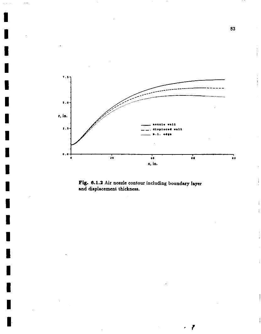
83

in.

1.1

0 . 0 4 I I I 1 6 0 8 0 20 4 0 0

x, in.

Fig. 6.1.3 Air nozzle contour including boundary layer and dieplacement thickness.

I I I

I 84 I

I I I I I I 1 I I I I I I I I I I

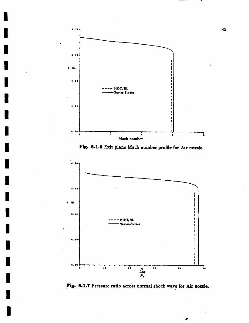
I I I I I I I I 1 I I I I I I I I I . I

9.21

0 . 1 !

r, m.

0 . 1 9

0 . 0 s

0 . 0 9

MOC/BL Narier- Stoker -

1 I I I I I I I I I I I I 1 I I I I I

9

I

a 4 I

Mach number

0 . 1 5

r, m.

9 . 1 0

0 . 0 s

0.0..

85

- 4

Fig. 6.1.1 Exit plane Mach number profiie for Air node.

I I I I I I I I I I I I I I I I I I I I I I I

MOC/BL ---- - N a r i ~ ~ S t o L a

IO 4 0 L O I 9 52 p.

1 5 0

Fie. 6.1.7 Pressure ratio across normal shock wave for Air node. - --

0

-1

-1

- 3

- 4

0 .

r, m.

0 .

0.0s

0 . 0 0

86

0 1 0 4 0 6 8 i o

Fig. 6.1.6 Centerline pressure ratio for Air nosale. x, in.

I I I I 1 I I I I I I I I I I I 1 I I I 1

10000

Fig. 6.1.8 Total pressure profile downstream of normal shock in exit plane of Air n o s h

I I I I 1 I I I I I I I I I I I I I I

87

I I

0

- 1

- 2

- 3

- 4 0

1.1

1 . 0

m

0 . S

0 . 0 0

- ~ O C / E L

_ _ . n a v i o r - a t o k o i

2 0 4 0

x, in.

Fig. 8.1.9 Wall pressure ratio for Air nozzle.

2 0 4 0 6 0

x, in.

Fig. 8.1.10 Navier-Stokes massflow rate for Air nozzle.

8 0

I O

1 0

r, in.

I

0

1 0

r, in

9

88

Fig. 6.2.1 Nl - 13 nozzle contour including b o u n d q lay- and displacement thickness.

v - - ' 1 - - - * . - . , . . . 1

6 0 8 0 1 0 0 1 2 8 1 4 0 1 0 4 0

x, in.

Fig. 6.2.3 N1 - 17 nozzle contour including boundary layer and displacement thickness.

I I I I I I

I I I

I I I I I I I I

- - - - - 0 . 2 5

89

1 1 1 1 I I I I 1 1 1 1 I l l 1 1 1 1 1 I I I I

1 0 -

r, in. *

s -

o . . - - , - - . . , . . . . l . . . . l . . . . l . . ~ - ~ L O O 12s 1 s o so x, in. 7 s 0

- - -

- 0 . 2 )

I I I

l l l l I I I I I I I I I l l 1 I 1 . 1 I I I I I

0 . 2 5 7

Fig. 6.2.3 Smoothed Na - 17 contour, slope and curvature.

1 1

2 0 I O 1 2 0 0

- - -

- 0 . 2 9 I I I I I I I 1

- - -

4. a s

Fig. 6.2.4 N2 - 13 contour, slope and curvatare.

4

I 1 I I I I I I

c -7-

I 90 I

I I I I I I 1 I I I I I I I I I I

I

I I I I I I I I I I I I I I I I I

~I I 91

92

- 1

1 . . . 1 - - - - 1 40 ( 0 I O A00 110 x, in. 0 2 8

Fig. 8.3.7 Centerline pressure ratio for Na - 13 nozzle.

I I

93

6 4 N

8 E t- r(

I

u c. (d c. ca

.C(

? 1 (0

.3 E

oi 4 N

0 8 t- w

I

-% E

a! 1 (0

.3 E

- 0 4 . - . , . . . , . . . 1 . . - 1 . . - , . - - 1 b0 0 0 l o @ i a a 1 4 @ 0 2 a 4 0

x, in. Fig. 6.1.10 Centerline pressure ratio for lVa - 17 nozzle (first wall temp.).

94

I I I I I I I I 1 I I I I I I I I 1 I

I

Fig. 6.3.13 Centerline pressure ratio for N2 - 17 n o d e (second wall temp.).

0

4 0

0 datapoint

0 gidpoint

A ineactionpokrt

Fig. 6.3.13 Movement of inflection point due to discretization.

95

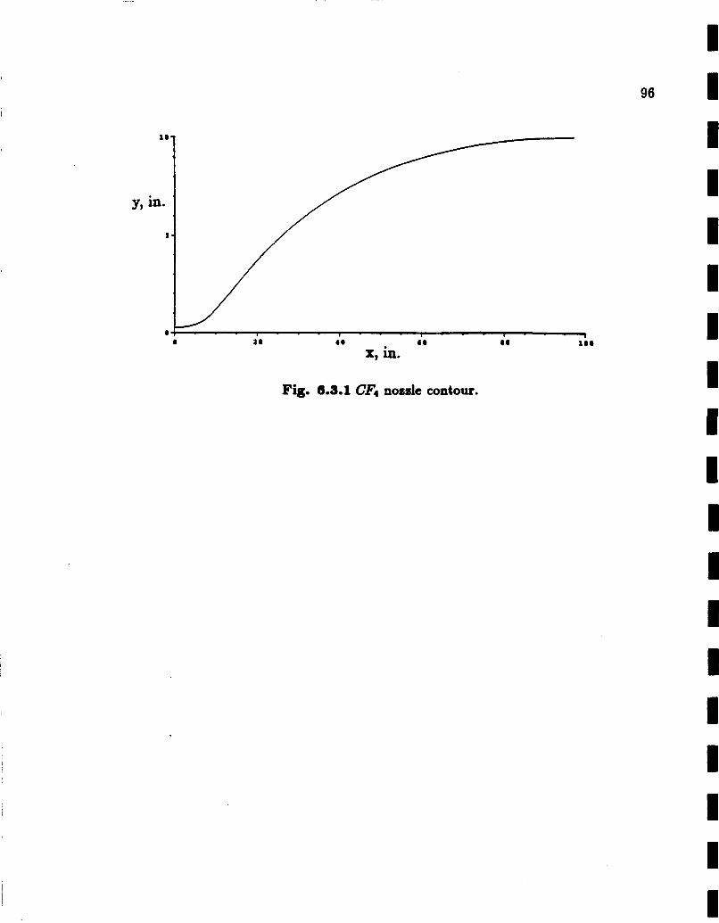
96

I I

Fig. 6.9.1 c8'. node contour.

I I

I I I I I I I I I I I I I I I I I I I

4 - - - - 0 . 2 9

97

I I I I I 1

1 0 -

r, in. '

S -

O I I I I I 2 0 4 0 x, in. 6 0 0 0 1 0 0 0

- - a . I ¶ I 1 I 1 I 1 I 1

Fig. 8.3.1 Smoothed C'! contour, slope and curvature.