Design and Implementation of an Efficient Parallel Feel ...

Purdue University Purdue University

Purdue e-Pubs Purdue e-Pubs

Department of Computer Science Technical Reports Department of Computer Science

2018

Design and Implementation of an Efficient Parallel Feel-the-Way Design and Implementation of an Efficient Parallel Feel-the-Way

Clustering Algorithm on High Performance Computing Systems Clustering Algorithm on High Performance Computing Systems

Weijian Zheng Indiana University - Purdue University, Indianapolis, [email protected]

Fengguang Song Indiana University Purdue University Indianapolis, [email protected]

Dali Wang Oak Ridge National Laboratory, [email protected]

Report Number: 18-002

Zheng, Weijian; Song, Fengguang; and Wang, Dali, "Design and Implementation of an Efficient Parallel Feel-the-Way Clustering Algorithm on High Performance Computing Systems" (2018). Department of Computer Science Technical Reports. Paper 1782. https://docs.lib.purdue.edu/cstech/1782

This document has been made available through Purdue e-Pubs, a service of the Purdue University Libraries. Please contact [email protected] for additional information.

https://docs.lib.purdue.edu/

https://docs.lib.purdue.edu/cstech

https://docs.lib.purdue.edu/cstech

https://docs.lib.purdue.edu/comp_sci

Design and Implementation of an EfficientParallel Feel-the-Way Clustering Algorithm on

High Performance Computing SystemsWeijian Zheng

Department of Computer SciencePurdue University

Indianapolis, [email protected]

Fengguang SongDepartment of Computer Science

Indiana University-Purdue UniversityIndianapolis, [email protected]

Dali WangOak Ridge National Laboratory

Oak Ridge, [email protected]

Abstract

This paper proposes a Feel-the-Way clustering method, which reducesthe synchronization and communication overhead, meanwhile providing asgood as or better convergence rate than the synchronous clustering methods.The Feel-the-Way clustering algorithm explores the problem space by usingthe philosophy of “crossing an unknown river by feeling the pebbles in theriverbed.” A full-step Feel-the-Way clustering algorithm is first designed toreduce the number of iterations. In the full-step Feel-the-Way algorithm, eachprocess runs a number of L steps before synchronizing its local solutions withother processes. This full-step algorithm can significantly decrease the numberof iterations compared to the k-means clustering method. Next, we extend thefull-step algorithm to a sampling-based Feel-the-Way algorithm to achievehigher performance. Furthermore, we prove that the proposed new algorithms(both full-step and sampling-based Feel-the-Way) can always converge. Ourempirical results demonstrate that the optimized sampling-based Feel-the-Waymethod is much faster than the widely used k-means clustering method aswell as providing comparable costs. A number of experiments with syntheticdatasets, real-world datasets of MNIST, CIFAR-10, ENRON, and PLACES-2show that the new parallel algorithm can outperform the k-means by up to235% on a high performance computing system with 2,048 CPU cores.

1. Introduction

Machine learning is a primary mechanism to extract infor-mation and insights from big data. It has recently generatedlarge amounts of momentous results in both academia andindustry. Owing to the large data volume, exponential rate ofdata generation and extreme-scale data processing, high per-formance computing (HPC) systems have become the standardplatform to solve machine learning problems at extreme scales.However, achieving high scalability for parallel and distributedmachine learning algorithms is still a challenging task.

This paper targets the k-means clustering method, which isone of the most widely used big data analytics methods today[1], [2]. It partitions a set of data points into k clusters by thefollowing two steps: 1) assign each data point to its closestcenter, and 2) recompute new centers as the means of thejust assigned points. The process is repeated for a number ofiterations until it converges. To achieve high performance on

This material is based upon research supported by the Purdue ResearchFoundation, by the NSF Grant# 1522554, and by the U.S. Department ofEnergy (DOE), Office of Science, Advanced Scientific Computing Research.

extreme-scale systems with millions of CPUs, it is crucial toreduce the communication cost and synchronization cost of aparallel algorithm. Researchers are conducting extensive stud-ies to design communication-reducing and synchronization-reducing machine learning algorithms [3], [4], [5], [6]. Thesealgorithms may reduce the communication cost and synchro-nization cost to speed up the execution time for each iteration.However, they sometimes cause a slower convergence rate(i.e., requiring more iterations), lower quality of solutions,or even divergence [7], [8], [9], [10]. Consequentially, theoverall execution time becomes longer since the increasednumber of iterations can overwhelm the benefits of improvedperformance per iteration.

Intrigued by this problem, we start to explore whether wecan design a set of new machine learning algorithms thatcan not only reduce the synchronization cost but also achievea better convergence rate. To that end, we design a newalgorithm named “Feel-the-Way” algorithm. The goal is toachieve the best of the two worlds: The new algorithm attainsminimized synchronizations meanwhile achieving the same orfaster convergence rate.

We design a Feel-the-Way Clustering algorithm to achievethe goal. The basic idea is that each computing processbehaves like a person who is trying to “cross an unknownriver by touching or feeling the pebbles/rocks in the riverbed.”In the design, the current rock is the safe “harbor” where theperson can always come back and try a new direction again.Note that many people are crossing the same river and willsynchronize from time to time. Following the idea, we designthe Feel-the-Way algorithm.

In the Feel-the-Way algorithm, each process has a subsetof the input dataset, and runs L local clustering steps beforesynchronizing its local solution with other processes’ localsolutions. Each process keeps track of its local solution (i.e.,k centers) for every local step from 1 to L. At the end of theL-th step, all processes’ local solutions are merged together todetermine a new global solution. Next, every process uses thenew global solution as a starting point, and repeats the samesteps until it converges. The rationale behind the idea is that

the solution from the first step is always a “decent” candidatefor the global solution. If one of the second, third, ..., and L-thsteps has a better optimization cost than the first step, it impliesthat the Feel-the-Way algorithm has successfully reducedsynchronizations and communications, meanwhile achieving abetter cost than the original synchronous algorithm. In general,the best of the L candidates will be at least as good as theoriginal synchronous algorithm in terms of the optimizationcost and the convergence rate. To understand it, consideringan extreme case, if all the local steps between the secondand the L-th make the cost worse than the first step, the finaloverall cost can still be close to the synchronous first-step-onlyclustering method because the first step is the “winner” whichis then adopted by the Feel-the-Way algorithm.

Our first attempt of realizing the new algorithm shows goodresults. Experiments in Section 6.2 demonstrate that usingL=5 can reduce the average number of iterations from 61to 10 with the MNIST dataset. However, it is not trivialto implement the algorithm in practice efficiently. To makeit run as fast as possible, we need to solve the followingchallenge: the time spent on the second to the L-th local stepsmust be significantly small to reduce the total execution time.Otherwise, the saved iterations may be overwhelmed by thetime of the second to L-th local steps. Hence, we consider thesecond to L-th local steps as an overhead we pay in order todecrease the number of iterations.

To reduce the overhead incurred by the second to L-thsteps, we use a variety of sampling methods to avoid re-clustering all the data points. Based on our analysis, notevery point is reassigned in the next iteration. Five samplingmethods have been designed and compared with each other:1) Random sampling, 2) a new Max-min sampling, 3) a newcoefficient of variation (CV) sampling, 4) Heap sampling [11],and 5) a new Reassignment-history-aware sampling method.These sampling algorithms have different time complexitiesand distinct efficiencies on the convergence rate. To integratethe Feel-the-Way clustering algorithm with the sampling al-gorithm, we also design a new approach to computing thesampling-based optimization cost efficiently for every locali-th step (i ∈ {2, . . . , L}). All the sampling methods arecontrolled by a sampling rate r, and each local step may havea different sampling rate. Finally, we call the new algorithm“sampling-based Feel-the-Way algorithm”. By contrast, theoriginal algorithm (i.e., without sampling) is called “full-stepFeel-the-Way algorithm”.

We first design and develop sequential algorithms for thefull-step Feel-the-Way algorithm and the sampling-based Feel-the-Way algorithm, respectively. The sequential algorithmspartition the input dataset into a number of data blocks, eachwith an equal number of data points. Then the algorithmsapply L local steps to each data block. Every local stepexecutes the k-means clustering method for one iteration uponthe data block. After all data blocks have been computed, thedata blocks’ centers will be merged to get new global centers.Given the new global centers, we repeat the same process.Note that the sampling-based algorithm only computes a

subset of points during the second to L-th local steps, butcomputes all points in the first local step.

After verifying the correctness of the sequential algorithms,we develop a parallel sampling-based Feel-the-Way algorithmusing the hybrid MPI/Pthread programming model. In theparallel implementation, every thread works on its own sub-set of data blocks, and merges centers with other threads.We conduct a number of experiments with synthetic datasets and real-world datasets of MNIST, CIFAR-10, ENRON,and PLACES-2 on HPC systems. The experimental resultsshow that the introduced reassignment-history-aware samplingmethod is more effective than the other sampling methods, andthe new parallel Feel-the-Way algorithm can outperform thek-means algorithm significantly. To the best of our knowledge,this paper makes the following contributions:

1) We propose a full-step Feel-the-Way algorithm and asampling-based Feel-the-Way algorithm to reduce syn-chronizations at the same time achieving as good as orbetter convergence rates.

2) We design a variety of sampling methods, among whichwe introduce the most effective reassignment-history-aware sampling method.

3) We prove that the sampling-based Feel-the-Way algo-rithm converges. We empirically show that the conver-gence rate is faster with the Feel-the-Way algorithm.

4) Our experiments with both sequential and parallel im-plementations using real-world datasets demonstrate thatthe Feel-the-Way method can provide faster performancethan the k-means method.

2. Related work

Existing machine learning libraries such as Mahout [12],Spark MLlib [13], Google TensorFlow [14], GraphLab [15]and Amazon AML [16] are general-purpose Big Data ecosys-tems. They target high productivity by using Python or Javaon Cloud platforms (e.g., Hadoop). For instance, Alex et al.found that Spark has significant runtime overhead (e.g. inter-stage barrier, task start delay, etc.) compared to MPI-basedsoftware [17]. Differently, this paper targets high performance[17], [18], and focuses on designing a new parallel clusteringalgorithm on HPC systems using the hybrid MPI/Pthreadprogramming model.

Numerous parallel ML algorithms on distributed memorysystems have been designed and developed: Some are strictlysynchronous but lead to significant communication cost, whilethe others use relaxed or lazy synchronizations but cannotguarantee the same convergence rate as the the original syn-chronous algorithms [7], [8], [9], [19], [20], [21]. Xing etal. study machine learning applications that use the stochasticgradient descent (SGD) algorithm, and adaptively change theSGD step size to compensate for errors caused by stalesynchronizations. Although we share the same philosophyof reducing synchronizations, our work focuses on clusteringmethods (i.e., not SGD related), and designs a distinct Feel-

2

the-Way algorithm to minimize both synchronization cost andthe number of iterations.

Mini-batch k-means clustering is a sampling-based cluster-ing algorithm [22]. It randomly selects a small number of datapoints from each batch. In this work, we test five differentsampling methods, and incorporate them (as a submodule)into the new Feel-the-Way algorithm. Note that our Feel-the-Way algorithm is a hybrid of sampling algorithm and ordinaryclustering algorithm, and can achieve the same optimizationcost as the original k-means. Kurban et al. design the heapmethod and use it to the k-means clustering method [11]. Wecompare the heap method with our reassignment-history basedmethod, and show that the reassignment-history-aware methodcan result in a better convergence rate than the heap method.

3. Full-Step Feel-the-Way Algorithm

This section introduces the proposed full-step Feel-the-Wayalgorithm, which works on blocks of data points and applieslocal optimizations to each individual block iteratively. Eachblock of data points will be optimized by a number of L localsteps without triggering any communications. The algorithmconsists of three parts: 1) The local optimization function thatiteratively optimizes each data block; 2) the merge functionthat derives the global clustering centers from different blocks;and 3) the main function that simply controls when to stopthe algorithm. The rest of the section will introduce the threefunctions in details.

3.1. Data structure

We use a blocked data layout to store the input dataset.In a machine learning application, each data point can berepresented by a vector with m attributes. Assuming we haven data points, a dataset can be viewed as an n-by-m matrix.In our algorithm, we divide the matrix into blocks of rows,where each block stores a set of b consecutive data points. Thisblocked data structure is used by both full-step and sampling-based Feel-the-Way algorithms.

3.2. Local optimization function

The local optimization function is in charge of reducingeach data block’s optimization cost. Its idea is as follows: werun one step of the synchronized algorithm (e.g., the originalk-means), then we run L-1 steps of asynchronous steps uponeach block. The additional L-1 steps on each data block aresupposed to reduce each block’s SSE (Sum of Squared Error)cost monotonically (Theorem 5.2 in Section 5 will prove it).

Algorithm 1 shows the pseudocode of the local optimizationfunction. The function goes through three stages. Stage 1: Setthe current data block’s clustering seed as the newly mergedglobal centers. Stage 2: Use the current data block’s points toimprove the block’s clustering cost. In stage 2.1, we find theclosest center for each data point; In stage 2.2, we computeeach block’s local centers’ sizes and sums of coordinates; In

Algorithm 1 Function of Local Optimization.

1: /∗ Local optimization on one block ∗/2: local optimization block(points, g centers,3: g centers size, membership, L)4: l = 0 /∗ l is the current step ∗/5: while l ≤ L− 1 do6: blk cost old = blk cost new; blk cost new = 0;7: blk local sum = 0; blk local size = 0;8: . stage 1: Use the global centers as a new seed for 0 step9: if (l = 0) then

10: centers ← g centers;11: end if12: . stage 2: Use all local points to improve centers13: for each point i in points do14: . stage 2.1 find the closest center for point i15: (dist, new center) ← find nearest center16: (points[i], centers);17: membership[i] = new center;18: . stage 2.2 update each block’s partial sum and size19: blk local sum[new center] += points[i];20: blk local size[new center]+=1;21: blk cost new += dist;22: end for23: . stage 2.3: Recalculate new centers and new cost24: for each center c do25: centers[c] = blk local sum[c] / blk local size[c];26: end for27: if (l = 0) then28: 1st step cost ← blk cost new;29: end if30: l++;31: end while32: . stage 3: Returns if L steps are finished33: return {blk local sum, blk local size, 1st step cost}

stage 2.3, we get new local centers based on step 2.2. Stage3: The local optimization function returns if a number of Llocal steps have been applied to the current data block.

3.3. The merge function

After calling the local optimization function, each data blockhas its own set of centers. Therefore, N data blocks willhave N set of centers. Given each data block’s local sum,local size and a new cost local cost, the merge function willadd them together to get the global sum and global size,respectively. The new global centers are then computed bydividing global sum by global size.

3.4. The main function

Algorithm 2 shows the main function of the full-step Feel-the-Way algorithm. It calls the previous local optimization andmerge functions. As shown in the algorithm, it first selects kpoints as the initial seed. Next, it iteratively optimizes eachdata block, and aggregates each clustering center’s size andcoordinate sum (see lines 12-20). After all the data blocks havebeen processed once, the new global centers can be computed(see lines 22-24).

3

Algorithm 2 Full-Step Feel-the-Way Algorithm

1: /∗ m : number of points , n b: number of blocks ∗/2: /∗ k centers , L: the limit for number of local steps ∗/3: Feel the Way clustering(points, m, n b, k, L)4: /* Set the initial k centers */5: pre g cost new = MAXIMUM6: repeat7: /* Store the previous iteration’s info */8: g size old = g size ne; g size new = 0;9: g sum new = 0;

10: pre g cost old = pre g cost new;11: pre g cost new = 0;12: for each block i ← 0 to n b - 1 do13: /* Run local optimization on each block */14: (local sum, local size, pre local cost) ←15: local optimization block(i-th block, g centers,16: g size old, membership, L);17: /* Merge each block’s coordinate sum into global sum */18: (g sum new, g size new, pre g cost new) ←19: merge(local sum, local size, pre local cost);20: end for21: /* Compute new global centers */22: for each center c do23: g centers[c] = g sum new[c] / g size new[c];24: end for25: until pre g cost new ≥ pre g cost old

4. Sampling-Based Feel-the-Way Algorithm

In this section, we first analyze the performance of thefull-step Feel-the-Way algorithm. Motivated by the unscalableperformance of the full-step algorithm, we then introducea sampling-based Feel-the-Way algorithm. We design andcompare five different types of sampling methods. Moreover,we introduce a new method to compute the new SSE costgiven only a small portion of reassigned data points.

4.1. Motivation for a new sampling-based algorithm

We evaluate the performance of the full-step Feel-the-Wayalgorithm on a synthetic dataset SYN (described in Table 4).Figure 1.a shows that the full-step Feel-the-Way algorithm cansignificantly reduce the number of iterations. For instance, k-means has 74 iterations while the full-step Feel-the-Way (whenL=5) has 17 iterations. However, in Figure 1.b, we find thatthe full-step Feel-the-Way is not faster than k-means whenL=4 and 5, even though Feel-the-Way has a less number ofiterations than k-means. The reason is that the time spenton the second to L-th local steps is expensive, which iseventually larger than the benefit of saved iterations. Laterin Lemma 5.5, we will prove that the full-step Feel-the-Wayalgorithm becomes slower than k-means if it takes more thanmL iterations to converge, where m is the number of iterationsthat the k-means algorithm takes.

Therefore, we hope to design a new algorithm, whichcan spend little time on the local steps (from the secondto the L steps), at the same time reducing the numberof iterations. Our in-depth analysis of tracking data pointstransitions between different clusters finds that, not all data

points have been reassigned to a distinct cluster. Also, fewerand fewer data points are reassigned from the first iterationto the last iteration. Intuitively, if we could just pick upthose reassigned points (and skip those unchanged points) tocompute, the Feel-the-Way algorithm can certainly run muchfaster. Hence, we introduce different sampling schemes to theoriginal Feel-the-Way algorithm’s local steps to intelligentlyselect a small portion of data points to compute clustering,instead of considering all data points (as done by the full-stepalgorithm).

4.2. Design of the sampling-based Feel-the-Way

The main function of the sampling-based Feel-the-Wayalgorithm is the same as the full-step Algorithm 2 except forthe local optimization function.

The new local optimization function is displayed in Algo-rithm 3. In lines 7-9, the sampling algorithm checks whetherit has visited enough data points or not. In line 10, onlythe sampled points will be selected to compute clustering.From line 11 to line 18, each sampled point is reassigned toits closest center, and those consequentially affected cluster’scoordinate sum and number of points are updated accordingly.Please note that this algorithm must consider all the data pointsas stated in line 10 when the algorithm executes the first localstep.

The essence of the Feel-the-Way algorithm is to use the firstlocal step to emulate the original synchronous k-means algo-rithm, and use the following L− 1 local steps to improve thecost of the first local step. Moreover, the sampling algorithmutilizes the first local step to compute the global SSE cost forall blocks of data points, and determines which points shouldbe sampled based upon the reassignment statistics of the firstlocal step.

4.3. Development of various sampling methods

We design and develop five different sampling methods.These sampling methods depend on one of two types ofinformation: 1) distance of the data point to each clusteringcenter (near or far), and 2) the history of previous steps thatreassign certain points to different centers.

The five sampling methods are as follows:

0

10

20

30

40

50

60

70

80

2 3 4 5

#it

era

tio

ns

L steps (within each iteration)

Full-step Feel-the-Way

k-means

(a) SYN (iterations)

0

0.2

0.4

0.6

0.8

1

1.2

2 3 4 5

Re

lati

ve

pe

rfo

rma

nce


Full-step Feel-the-Way k-means

(b) SYN (speedup)

Fig. 1: Comparison between the full-step Feel-the-Way algo-rithm and the k-means algorithm.

4

Algorithm 3 Sampling Version of the Local OptimizationFunction

1: /∗ Local optimization on one block ∗/2: local optimization block(points, g centers,3: g centers size, membership, L, max sample points)4: /*same as lines 4-11 of Algorithm 1) */5: . stage 2: Use sampled local points to improve centers6: for each point i in points do7: if (sampled points > max sample points) then8: break;9: end if

10: if (point i is sampled or local step = 0) then11: sampled points = sampled points + 1;12: . stage 2.1 find the closest center for point i13: (dist, new center) ← find nearest center14: (points[i], centers);15: membership[i] = new center;16: . stage 2.2 update each block’s partial sum and size17: blk local sum[new center] += points[i];18: blk local size[new center]+=1;19: if (l != 0 ) then20: blk local sum[old center] -= points[i];21: blk local size[old center]-=1;22: end if23: end if24: end for25: /*same as local optimization function (i.e., Alg. 1) lines 23-33*/

1) Random sampling: It randomly selects a subset of datapoints.

2) Max-min sampling: For each data point, we compute itsdistances to the k clustering centers, respectively. Thenwe compute its Max-min (i.e., max distance

min distance ). Those pointsthat have smaller Max-min values will be selected as thesampling points. It is based on our assumption that if adata point is equally close to all k centers, it is morelikely this point will change its closest center.

3) Coefficient of Variation (CV): CV is defined asstandard deviation

mean . For each data point, there are k distancesto k centers. This method computes the CV of those kdistances. A small CV reveals that the distances of thedata point to all centers are almost the same. Hence, thedata points that have smaller CVs will be selected byassuming that a point with comparable distances to allcenters is likely to be reassigned soon.

4) Heap sampling: Heap based sampling is inspired by thework of Kurban et al. [11]. The heap based methodmaintains a heap data structure for each center to storethe distances between the center and its data points. Thefarthest data point is stored at the top of the heap (similarto heap sorting). When doing sampling, we always selectthe points that are at the upper levels of the heap. Theheap method assumes that the points that are far fromtheir belonging center will switch to a new center morequickly.

5) Reassignment-history-aware sampling: It is a new sam-pling method proposed by this work. Reassignment-history-aware sampling tries to keep track of which data

points have been reassigned in the past. If a data pointis assigned to a new center in the previous step, weconsider it as a sampling point candidate by assumingit will change center again in the current step. Supposethere are m data points that have been assigned to newcenters in the previous step, we will randomly pick ssample points from the set of m points. s is eithera constant or decided by a sampling ratio. When mbecomes too small (e.g., less than 20), we will use allm points as the sampling points.

Time complexity of the sampling methods: In the aboveMax-min, CV, and Heap sampling methods, we use the Quick-Select algorithm [23] to find the first s numbers (either largestand smallest) in an array. QuickSelect has a time complexityof O(logn). Given k centers and each data block with b datapoints, we summarize the time complexities of all the samplingmethods in Table 1 (proofs are skipped here). Here, we assumethat each sampling method needs to select s sample pointsfrom each data block.

TABLE 1: Time complexity of different sampling methods.

Random Max-min Heap CV Reassignment-history-aware

O(s) O(s log b) O(sk log bk

) O(s log b) O(s)

4.4. An efficient way to compute the new SSE costin the sampling algorithm

For each local step l (l ∈ {1 . . . L−1}) for which samplingis needed, we will compute the new SSE cost at the endof the l-th local step. Certainly we cannot recompute everypoint’s distance to its center because of its expensive cost,which would make the sampling algorithm have the same timecomplexity of the full-step algorithm.

In order to compute a new SSE cost by considering onlythe small subset of sampling points, we divide the SSE costcomputation into two parts: 1) SSE cost related to the sampledpoints, and 2) SSE cost related to the upsampled points.

Suppose V represents all the points in a data block, andS and U represent sampled points and upsampled points,respectively, where V = S ∪ U .cost(S) (i.e., the cost of the sampled data points) is the SSE

cost of the sampled point. It is computed when each sampledpoints is reassigned to its closest center.

Next, the SSE cost of unsampled points cost(U) is com-puted as follows. We utilize the old SSE cost of unsampleddata points cost(U)old to compute the new cost of unsampleddata points. Specifically, given a set of centers C from theprevious local step, after re-clustering, we get a new set ofcenters C ′. For unsampled data point U , we also record the co-ordinates sums and the number of data points attached to eachcenter in previous step as sum and size. Let σi = C ′i − Ci,where Ci is the i-th center. The corresponding computationformula is as follows: cost(U) = cost(U)old−2

∑ki=1(sumi−

sizei · Ci) · σi +∑ki=1(sizei(σi · σi)).

5

Eventually, cost(V ) = cost(S) + cost(U).

5. Theoretical Analysis

In this section, we will analyze the proposed Feel-the-Wayalgorithm, and provide theorems and lemmas to answer twoquestions: 1) Does the sampling-based Feel-the-Way algorithmalways converge (subsection 5.1)? 2) In what conditions theFeel-the-Way algorithm will be faster than the k-means method(subsection 5.2)?

5.1. Convergence analysis

Clustering problems study how to partition a set of datapoints T—which has a number of n points in a d-dimensionspace (<d)—into k groups with the minimum cost. Let µ be adata point in <d, and the result of clustering is a membershipvector M and a set of centers C.

Since we use a blocking data structure, T is divided into anumber |T |b of blocks. Assume V is a block with b data pointsand there are L local steps within one global iteration. Givenblock V , in each local step l ∈ [0, L−1], the local optimizationfunction is invoked to minimize the block V ’s own SSE costcost(V,C ′), where C ′ is the current best centers of the block.We also know that cost(V,C ′) =

∑µ∈V dist(µ − C ′M(µ)).

C ′M(µ) is the closest center among C ′ to the point µ.Given two data points x and y, the squared Euclidean

distance between them, ∆(x, y), can be computed as follows:∆(x, y) =

∑di=1(xi − yi)2 = (x − y) · (x − y) (i.e., a dot

product).

Lemma 5.1. Given an initial set of centers C (|C| = k)for block V , after reassignment of each data point in V toits closest center, we get a new membership M ′. Supposemembership M ′ implies a new set of centers C ′, the newcenters C ′ always has a cost that is equal to or less than that ofthe old centers C. That is, cost(V,C,M ′) ≥ cost(V,C ′,M ′).

Proof: Let σi = C ′i − Ci, where Ci is the i-th center.

cost(V,C,M ′) =∑µ∈V

∆(µ,CM′(µ)) /*by definition of SSE cost*/

=∑µ∈V

(µ− C′M′(µ) + σM′(µ)) · (µ− C′M′(µ) + σM′(µ))

=∑µ∈V

(∆(µ,C′M′(µ)) + 2(µ− C′M′(µ)) · σM′(µ) + (σM′(µ))2)

= cost(V,C′,M ′) + 2

k∑m=1

(σm ·∑

µ∈V,M′(µ)=m

(µ− C′m))

+∑µ∈V

(σM′(µ))2 = cost(V,C′,M ′) +

∑µ∈V

(σM′(µ))2

(1)

Note that∑µ∈V,M ′(µ)=m(µ − C ′m) is zero since C ′m is a

center of a cluster of points (i.e., the arithmetic mean positionof all the points in the m-th cluster).

Lemma 5.2. Let cost(V,Cl, M l) and cost(V,Cl+1, M l+1)be the computed SSE cost for block V before and after thel-th local step, then cost(V,Cl, M l) ≥ cost(V,Cl+1, M l+1).

Proof: In the l-th local step, every data point will bereassigned to its closest center such at a lower cost is achievedand a new membership of the points is formed, because eachreassigned point’s distance (to its new center) has decreased.Thus, cost(V,Cl,M l) ≥ cost(V,Cl,M l+1).

The new membership M l+1 leads to a new set of centers,denoted as Cl+1. Based on Lemma 5.1, cost(V,Cl,M l+1)≥ cost(V,Cl+1,M l+1). Putting two inequalities together,cost(V,Cl,M l) ≥ cost(V,Cl+1,M l+1).

Lemma 5.2 shows that each data block’s SSE cost willdecrease monotonically in each local l-th step. Lemma 5.2is still correct even if we only consider reassignment of a setof sampled points, for which every point in the proof refers toevery sampled point and the unsampled points do not affect(i.e., increase/decrease) the SSE cost.

Lemma 5.3. Suppose an input dataset T is divided intoP data blocks. Each data block Vi has its own clusteringmembership MVi and a set of k centers CVi . After mergingall the blocks’ local centers into a global set of centers CT ,cost(T,CT ,MT ) ≤

∑Pi=1 cost(Vi, CVi

,MVi).

Proof: Let σi = CT (i) − C(i), where CT (i) is the i-thglobal center. C(i) here is approximately equal to the i-thcenter of each block. µ is a single data point.

P∑i=1

cost(Vi, CVi,MVi

) =P∑i=1

∑µ∈Vi

∆(µ− CVi(MVi(µ)))

=

P∑i=1

∑µ∈Vi

((µ− CT (MVi(µ)) + σMVi

(µ))

· (µ− CT (MVi(µ)) + σMVi

(µ)))

=

P∑i=1

cost(Vi, CT ,MVi) +

P∑i=1

∑µ∈Vi

(σMVi(µ))

2

+ 2

k∑m=1

(σm ·P∑i=1

∑µ∈Vi,MVi

(µ)=m

(µ− CT (m)))

= cost(T,CT ,MT ) +

P∑i=1

∑µ∈Vi

(σMT (µ))2

(2)

Please note that∑Pi=1

∑µ∈Vi,MVi

(µ)=m(µ − CT (m)) iszero since CT (m) is a center of a cluster points based onmembership MVi

.

Theorem 5.4. Let cost(T,Ci−1T ,M i−1T ) and cost(T,CiT ,M

iT )

be the computed global SSE cost for all data points T beforeand after the i-th global iteration, then cost(T,Ci−1T ,M i−1

T )≥ cost(T,CiT ,M

iT ).

Proof: Assume there are l local steps inside one globaliteration. Let Ci(l−1)V and M

i(l−1)V be the local center and

membership of V after l-th step within i-th iteration. M i(l−1)T

6

is the membership of all data points copied from Mi(l−1)Vm

. LetCiT be the merged global center after i-th iteration. M i

T is themembership of all data points implied by CiT

cost(T,Ci−1T ,M i−1

T ) =

P∑m=1

cost(Vm, Ci(0)Vm

,Mi(0)Vm

)

≥P∑

m=1

cost(Vm, Ci(l−2)Vm

,Mi(l−2)Vm

) /* According to lemma 5.2 */

≥P∑

m=1

cost(Vm, Ci(l−2)Vm

,Mi(l−1)Vm

) /* Find the closest center */

≥ cost(T,CiT ,Mi(l−1)T ) /* According to lemma 5.3 */

≥P∑

m=1

cost(Vm, CiT ,M

iT ) /* Find the closest center */

= cost(T,CiT ,MiT )

(3)

Thus, cost(T,Ci−1T ,M i−1T ) ≥ cost(T,CiT ,M i

T )

Theorem 5.4 shows that the algorithm’s global cost ismonotonically decreasing, and the sampling-based Feel-the-Way algorithm converges.

5.2. Speedup analysis for the full-step and sampling-based Feel-the-Way algorithms

Lemma 5.5 (Full-step). Assume it takes m and n iterationsfor the k-means and the full-step Feel-the-Way algorithm toconverge. Let Tk−means and Tfull−step be the computationtime of the k-means and full-step Feel-the-Way algorithm,respectively. If n ≤ m

L , then Tfull−step ≤ Tk−means.Proof: Assume each iteration takes time t,

Tk−means ≥ Tfull−step =⇒ t×m ≥ t× n× L

=⇒ m ≥ n× L(4)

Thus, when n ≤ mL

, Tfull−step ≤ Tk−means.

Theorem 5.6 (Sampling-based). Assume it takes m and niterations for k-means and the sampling-based Feel-the-Wayalgorithm to converge. Suppose the sampling Feel-the-Wayalgorithm uses a sampling ratio of r. Let Tk−means andTsample be the computation time of the k-means and sampling-based Feel-the-Way algorithm, respectively. If n ≤ m

1+(L−1)r ,then Tsample ≤ Tk−means.

Proof: Assume the time for each iteration is t

Tk−means ≥ Tsample =⇒ t×m ≥ (t+ (L− 1)× r × t)× n

=⇒ m ≥ n× (1 + (l − 1)× r)(5)

Thus, Tsample ≤ Tk−means when n ≤ m1+(l−1)r

.Theorem 5.6 reveals that the speedup of the sampling-based

Feel-the-Way over k-means is determined by the reducednumber of iterations, the number of local steps, and thesampling ratio. For instance, if we choose L = 2 and asmall r, the sampling-based algorithm should be faster thank-means. Experimental results in Section 6.2 will demonstrate

the speedup of the sampling-based Feel-the-Way algorithm, inwhich we set r=1%.

6. Experimental Results

In this section, we will show three sets of experimentalresults on both synthetic and real-world datasets to evaluate theperformance of our algorithms and implementation: 1) In thefirst set of experiments, we evaluate the effectiveness of differ-ent sampling methods; 2) In the second set of experiments, wecompare the performance of k-means, full-step and sampling-based Feel-the-Way algorithms in terms of wallclock time andnumber of iterations; and 3) In the last set of experiments, weevaluate the scalability of our parallel implementation usingthousands of CPU cores. Note that in all of the experiments,we use double precision floating point numbers and four-bytesintegers to do the computations.

Computing Platform: We performed experiments on theBigRed II system located at the Indiana University. BigRedII is a Cray XE6/XK7 HPC system, which consists of 1,020compute nodes. Each compute node has two 16-core CPUsand 64GB of memory. Table 2 shows detailed information ofthe system.

TABLE 2: The BigRed II Supercomputer System.

Nodes 1,020 (max 2048 cores per job)Memory per node 64 GBProcessors per node 2Cores per processor 16Processor AMD Opteron 6380 2.5GHzInterconnect Cray GeminiMPI Cray-MPICH 7.2.5

Datasets: We use four real-world datasets, and two syn-thetic datasets. Table 3 shows the information of the four real-world datasets, which are MNIST, CIFAR-10, ENRON, andPLACES-2. MNIST is a well-known dataset for hand-writingdigit recognition [24]. CIFAR-10 is used for object recognitionwith 60,000 color images [25]. PLACES-2 is generated fromPlaces 2 [26], which is a large collection of images fromdifferent scenarios. ENRON is a dataset of documents andwas initially used for the email classification research [27].

We also use two synthetic datasets in our experiments.Table 4 shows the two synthetic datasets, which are namedSYN and SYN-Large. We generate the synthetic datasets usingdifferent Gaussian distributions. In particular, the larger datasetof SYN-Large is generated to measure the scalability of ourparallel implementation with many CPUs.

For each experiment, we use five different seeds, and reportthe average of the measured performances as our performanceresult. Also, all the Feel-the-Way experiments have compara-ble SSE costs to the k-means algorithm.

6.1. Comparison of Various Sampling Methods

As described in Section 4.3, the sampling-based Feel-the-Way algorithm deploys a sampling approach to the 2nd to

7

TABLE 3: Specifications of the real-world datasets.

MNIST CIFAR-10 ENRON PLACES-2K 10 10 10 50#Data points 10,000 60,000 38,400 1,024,000#Coordinates 784 3,072 28,102 1,024Dataset size 17MB 626MB 24.7MB 3.25GB

TABLE 4: Specifications of the synthetic datasets.

SYN SYN-LargeK 10 10

#Data points 6,400 204,800#Coordinates 1,024 2,048Dataset size 50.48MB 3.23GB

the L-th steps, while computing the whole set of points forthe first step. Since the effectiveness of the sampling methoddetermines the performance of sampling-based Feel-the-Way,we compare and evaluate five different sampling methods: 1)Random, 2) Max-min, 3) Coefficient of Variation (CV), 4)Heap, and 5) Reassignment-history-aware method (in short,Reassign-hist).

In the rest of the subsection, we use the Reassignment-history-aware method as an example to explain how a sam-pling ratio will affect the convergence rate and execution time.Next, we use a selected small ratio of 1% to compare fivesampling methods.

Effect of the sampling ratio. We use the parameter ofsampling ratio to control how many data points should beconsidered to compute new clustering centers. If the samplingratio is p%, p% of the total number of points will be accessedby the algorithm.

0

2

4

6

8

10

12

14

0

5

10

15

20

25

30

0.01 0.1 0.2 0.3 0.4 0.5 0.6 0.7 0.8 0.9 1

Tim

e (

s)

#ite

rati

on

s

Sampling ratio

Sampling-based Feel-the-Way (iterations)

Sampling-based Feel-the-Way (time)

k-means (time)

Fig. 2: Effect of the sampling ratio with the MNIST datasetusing the Reassignment-history-aware sampling method.

Figure 2 shows how the number of iterations and theexecution time will change as the sampling ratio increasesfrom 1% to 100% for the MNIST dataset. Here we usethe Reassignment-history-aware sampling and set L = 4 totest the Feel-the-Way algorithm. Regarding the number ofiterations, when the sampling ratio = 1%, Feel-the-Way takes27 iterations. Then, the number of iterations drops slowly from27 to 21 as the ratio rises from 1%, 10% to 80%. Eventually,

when the sampling ratio is equal to 90%, we see a significantdrop in the number of iterations. This experiment tells us thatgiven a specific sampling method, making the sampling ratiosmaller does not necessarily degrade the number of iterationsgreatly (e.g., 20%, 10%, 1% have nearly the same number ofiterations).

On the other hand, the execution time increases morequickly than the speed in which the number of iterationsdecreases (except for 90% and 100%). For instance, theexecution time jumps quickly from 4 seconds to 12 secondswhen the ratio rises from 1% to 80%. This is because a largersampling ratio implies a larger time complexity for each localstep l (l = 2, 3, 4). Theorem 5.6 has proved a formula todescribe the relationship between time and the number ofiterations given a specific L.

Since our goal is to optimize the execution time, we chooseto use a small sampling ratio of 1% by bringing in two benefits:1) It can lead to a small overhead (around 1%) to computemost local steps l ∈ {2 . . . L}; and 2) In combination withthe first full step of l = 1, the sampling-based Feel-the-Wayalgorithm can achieve a less number of iterations than k-means(i.e., 27 iterations versus k-means’ 61.4 iterations, on average).

Comparison of the five sampling methods. Next, we testwhich sampling method can provide the best performance. Ourevaluation is based on two metrics: 1) Accuracy. If a samplingmethod selects s data points, we measure how many pointsof the selected points have really been assigned to a differentcluster (e.g., h points switched clusters). We use h

s to representthe accuracy of the sampling method. We call it “Sampling HitRate”. The higher the sampling hit rate, the better the samplingmethod is. The second metric is 2) the number of iterationsneeded by the Feel-the-Way clustering algorithm to eventuallyconverge.

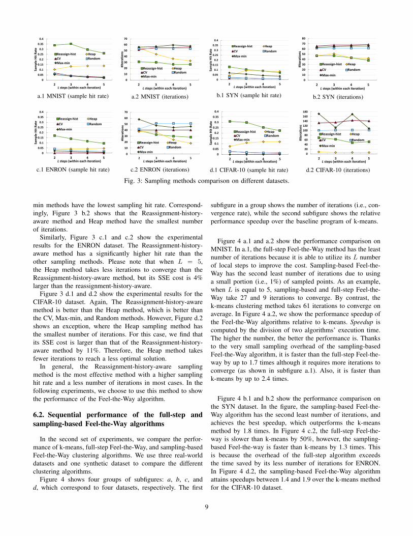
In Figure 3, we show the experimental results with fourdatasets: MNIST, SYN, ENRON, and CIFAR-10. For eachdataset, we evaluate different sampling methods’ sampling hitrate and number of iterations, respectively.

As shown in Figure 3 a.1, the Reassignment-history-awaremethod has the best sampling hit rate of 35% when L = 2and 3. The hit rate lowers to 30% and 25% when L = 4and 5. The second best sampling method is the Heap method,which has a sampling hit rate of 15%. The other three methods(Random, CV, and Max-min) only achieve sampling hit ratesthat are less than 5%. From the perspective of convergencerate, Figure 3 a.2 shows that the Reassignment-history-awaremethod is the fastest one, taking around 30 iterations. TheMax-min sampling method takes 60 iterations, and the CV,Random sampling methods take 51 and 53 iterations. TheHeap sampling method converges slowly when L = 2, butstarts to converge faster when L is bigger. Note that thesampling method that has a higher hit rate is more likely toconverge faster.

Figure 3 b.1 shows the SYN dataset’s sampling hit rate.When L > 2, the heap method is as good as the thereassignment-history-aware method. The Random and Max-

8

0

0.05

0.1

0.15

0.2

0.25

0.3

0.35

0.4

2 3 4 5

Sam

ple

Hit

Rat

e


Reassign-hist Heap

CV Random

Max-min

a.1 MNIST (sample hit rate)

0

10

20

30

40

50

60

70

2 3 4 5

#ite

rati

on

s


Reassign-hist HeapCV RandomMax-min

a.2 MNIST (iterations)

0

0.05

0.1

0.15

0.2

0.25

0.3

0.35

0.4

2 3 4 5

Sam

ple

Hit

Rat

e


Reassign-hist Heap

CV Random

Max-min

b.1 SYN (sample hit rate)

0

10

20

30

40

50

60

70

80

2 3 4 5

#ite

rati

on

s


Reassign-hist Heap

CV Random

Max-min

b.2 SYN (iterations)

0

0.05

0.1

0.15

0.2

0.25

0.3

0.35

0.4

2 3 4 5

Sam

ple

Hit

Rat

e


Reassign-hist Heap

CV Random

Max-min

c.1 ENRON (sample hit rate)

0

10

20

30

40

50

60

70

2 3 4 5

#ite

rati

on

s


Reassign-hist Heap

CV Random

Max-min

c.2 ENRON (iterations)

0

0.05

0.1

0.15

0.2

0.25

0.3

0.35

0.4

2 3 4 5

Sam

ple

Hit

Rat

e


Reassign-hist HeapCV RandomMax-min

d.1 CIFAR-10 (sample hit rate)

0

20

40

60

80

100

120

140

160

180

2 3 4 5

#ite

rati

on

s


Reassign-hist Heap

CV Random

Max-min

d.2 CIFAR-10 (iterations)

Fig. 3: Sampling methods comparison on different datasets.

min methods have the lowest sampling hit rate. Correspond-ingly, Figure 3 b.2 shows that the Reassignment-history-aware method and Heap method have the smallest numberof iterations.

Similarly, Figure 3 c.1 and c.2 show the experimentalresults for the ENRON dataset. The Reassignment-history-aware method has a significantly higher hit rate than theother sampling methods. Please note that when L = 5,the Heap method takes less iterations to converge than theReassignment-history-aware method, but its SSE cost is 4%larger than the reassignment-history-aware.

Figure 3 d.1 and d.2 show the experimental results for theCIFAR-10 dataset. Again, The Reassignment-history-awaremethod is better than the Heap method, which is better thanthe CV, Max-min, and Random methods. However, Figure d.2shows an exception, where the Heap sampling method hasthe smallest number of iterations. For this case, we find thatits SSE cost is larger than that of the Reassignment-history-aware method by 11%. Therefore, the Heap method takesfewer iterations to reach a less optimal solution.

In general, the Reassignment-history-aware samplingmethod is the most effective method with a higher samplinghit rate and a less number of iterations in most cases. In thefollowing experiments, we choose to use this method to showthe performance of the Feel-the-Way algorithm.

6.2. Sequential performance of the full-step andsampling-based Feel-the-Way algorithms

In the second set of experiments, we compare the perfor-mance of k-means, full-step Feel-the-Way, and sampling-basedFeel-the-Way clustering algorithms. We use three real-worlddatasets and one synthetic dataset to compare the differentclustering algorithms.

Figure 4 shows four groups of subfigures: a, b, c, andd, which correspond to four datasets, respectively. The first

subfigure in a group shows the number of iterations (i.e., con-vergence rate), while the second subfigure shows the relativeperformance speedup over the baseline program of k-means.

Figure 4 a.1 and a.2 show the performance comparison onMNIST. In a.1, the full-step Feel-the-Way method has the leastnumber of iterations because it is able to utilize its L numberof local steps to improve the cost. Sampling-based Feel-the-Way has the second least number of iterations due to usinga small portion (i.e., 1%) of sampled points. As an example,when L is equal to 5, sampling-based and full-step Feel-the-Way take 27 and 9 iterations to converge. By contrast, thek-means clustering method takes 61 iterations to converge onaverage. In Figure 4 a.2, we show the performance speedup ofthe Feel-the-Way algorithms relative to k-means. Speedup iscomputed by the division of two algorithms’ execution time.The higher the number, the better the performance is. Thanksto the very small sampling overhead of the sampling-basedFeel-the-Way algorithm, it is faster than the full-step Feel-the-way by up to 1.7 times although it requires more iterations toconverge (as shown in subfigure a.1). Also, it is faster thank-means by up to 2.4 times.

Figure 4 b.1 and b.2 show the performance comparison onthe SYN dataset. In the figure, the sampling-based Feel-the-Way algorithm has the second least number of iterations, andachieves the best speedup, which outperforms the k-meansmethod by 1.8 times. In Figure 4 c.2, the full-step Feel-the-way is slower than k-means by 50%, however, the sampling-based Feel-the-way is faster than k-means by 1.3 times. Thisis because the overhead of the full-step algorithm exceedsthe time saved by its less number of iterations for ENRON.In Figure 4 d.2, the sampling-based Feel-the-Way algorithmattains speedups between 1.4 and 1.9 over the k-means methodfor the CIFAR-10 dataset.

9

0

10

20

30

40

50

60

70

2 3 4 5

#ite

rati

on

s


Sampling-based Feel-the-Way


k-means

a.1 MNIST (iterations)

0

0.5

1

1.5

2

2.5

2 3 4 5

Re

lati

ve p

erf

orm

ance


Sampling-based Feel-the-WayFull-step Feel-the-Wayk-means

a.2 MNIST (speedup)

0

10

20

30

40

50

60

70

80

2 3 4 5

#ite

rati

on

s




k-means

b.1 SYN (iterations)

0

0.5

1

1.5

2

2 3 4 5

Re

lati

ve P

erf

orm

ance



b.2 SYN (speedup)

0

10

20

30

40

50

60

2 3 4 5

#ite

rati

on

s




k-means

c.1 ENRON (iterations)

0

0.5

1

1.5

2 3 4 5

Re

lati

ve P

erf

orm

ance



c.2 ENRON (speedup)

0

20

40

60

80

100

120

140

2 3 4 5

#ite

rati

on

s




k-means

d.1 CIFAR-10 (iterations)

0

0.5

1

1.5

2

2 3 4 5

Re

lati

ve P

erf

orm

ance



d.2 CIFAR-10 (speedup)

Fig. 4: Performance comparison on different datasets

1,035.0 566.0

298.1 160.4

80.3 40.7

709.6 395.0

216.6 123.5

62.6 32.3

1

10

100

1000

10000

1 2 4 8 16 32

tim

e (

s)

#cores

k-means


(a) ENRON

451.9 233.4

123.1 64.8

32.6 16.5

8.5 4.4

219.1 116.2

62.3 34.1

17.3 8.9

4.6 2.5

1

10

100

1000

1 2 4 8 16 32 64 128

tim

e (

s)

#cores

k-means


(b) CIFAR-1057.1

28.9

14.6

7.5

4.0

2.3

32.7

16.8

8.6

4.5

2.5 1.5

1

10

100

32 64 128 256 512 1024

tim

e (

s)

#cores

k-means


(c) SYN-Large

310.3 155.3

78.0 39.3

20.0 10.2

5.4

160.6 80.9

40.7 20.7

10.3 5.5

3.3

1

10

100

1000

32 64 128 256 512 1024 2048

tim

e (

s)

#cores

k-means


(d) PLACES-2

Fig. 5: Strong scalability experiments. The y-axis is shown inthe logarithmic scale.

6.3. Scalability of the parallel sampling-based Feel-the-Way algorithm

Finally, we perform large scale experiments to evaluate thescalability of our parallel implementation for the sampling-based Feel-the-Way algorithm. In the parallel experiments, wetake as input four datasets: ENRON, CIFAR-10, SYN-Large,and PLACES-2.

Figure 5 shows the performance of strong scalability. Aswe increase the number of CPU cores, the execution time willdecrease correspondingly. Figure 5.a displays the executiontime of k-means and sampling-based Feel-the-Way on theENRON dataset. As the number of CPU cores increases from1 to 32, our parallel Feel-the-Way reduces the execution timefrom 709.6 to 32.3 seconds while k-means reduces it from

1,035 to 40.7 seconds. Figure 5.b displays the execution timewhen using the CIFAR-10 dataset. On 128 CPU cores, ourparallel implementation is faster than k-means by 176%.

In Figure 5.c, we use 1,024 CPU cores to compute the SYN-Large dataset. From the subfigure c, we can see that the par-allel Feel-the-Way implementation reduces the execution timefrom 32.7 to 1.5 seconds using 1,024 cores, outperforming k-means by 153%. As for the PLACES-2 dataset as shown in(d), the wallclock execution time is decreased from 160.6 to3.3 seconds when using a number of 2,048 CPU cores. Theparallel sampling-based Feel-the-Way implementation is ableto outperform the k-means method by 164%.

7. Conclusion

In this paper, we seek to design and develop a fast clusteringalgorithm for large-scale HPC systems. We first design thefull-step Feel-the-Way algorithm. Compared to k-means, thisalgorithm takes significantly less number of iterations byapplying local optimization to each data block, meanwhileproviding the same cost as the k-means algorithm. Next,to optimize the execution time of the full-step algorithm,we introduce different sampling methods and design a newalgorithm called sampling-based Feel-the-Way. By samplinga few useful data points, the new sampling-based algorithmhas a much better performance than the full-step algorithm.Five sampling methods are designed and tested, among whichthe reassignment-history-aware sampling method achieves thebest convergence rate. Our future work along this line willdesign sampling-based parallel Feel-the-Way algorithms forother machine learning and deep learning methods on extreme-scale HPC systems.

References

[1] A. K. Jain, M. N. Murty, and P. J. Flynn, “Data clustering: a review,”ACM computing surveys (CSUR), vol. 31, no. 3, pp. 264–323, 1999.

10

[2] J. A. Hartigan and J. Hartigan, Clustering algorithms. Wiley New York,1975, vol. 209.

[3] A. Frommer and D. B. Szyld, “On asynchronous iterations,” Journal ofcomputational and applied mathematics, vol. 123, no. 1, pp. 201–216,2000.

[4] J. W. Demmel, L. Grigori, M. F. Hoemmen, and J. Langou,“Communication-optimal parallel and sequential QR and LU factoriza-tions,” UTK, LAPACK Working Note 204, August 2008.

[5] R. Bru, L. Elsner, and M. Neumann, “Models of parallel chaotic iterationmethods,” Linear Algebra and its Applications, vol. 103, pp. 175–192,1988.

[6] F. Song, H. Ltaief, B. Hadri, and J. Dongarra, “Scalable tilecommunication-avoiding QR factorization on multicore cluster sys-tems,” in Proceedings of the 2010 ACM/IEEE International Conferencefor High Performance Computing, Networking, Storage and Analysis(SC’10), 2010, pp. 1–11.

[7] Q. Ho, J. Cipar, H. Cui, S. Lee, J. K. Kim, P. B. Gibbons, G. A.Gibson, G. Ganger, and E. P. Xing, “More effective distributed ML viaa stale synchronous parallel parameter server,” in Advances in neuralinformation processing systems, 2013, pp. 1223–1231.

[8] M. G. Tallada, “Coarse grain parallelization of deep neural networks,”in ACM SIGPLAN Notices, vol. 51, no. 8. ACM, 2016, p. 1.

[9] W. Zheng, F. Song, and L. Lin, “Designing a synchronization-reducingclustering method on manycores: Some issues and improvements,” inProceedings of the Machine Learning on HPC Environments. ACM,2017, p. 9.

[10] S. Shi, Q. Wang, P. Xu, and X. Chu, “Benchmarking state-of-the-artdeep learning software tools,” in 7th International Conference on CloudComputing and Big Data (CCBD). IEEE, 2016, pp. 99–104.

[11] H. Kurban and M. M. Dalkilic, “A novel approach to optimization ofiterative machine learning algorithms: Over heap structure,” in 2017IEEE International Conference on Big Data (Big Data). IEEE, 2017,pp. 102–109.

[12] Apache Mahout, “https://mahout.apache.org/,” 2017.[13] MLlib, “http://spark.apache.org/mllib/,” 2017.[14] M. Abadi, A. Agarwal, P. Barham, E. Brevdo, Z. Chen, C. Citro, G. S.

Corrado, A. Davis, J. Dean, M. Devin et al., “Tensorflow: Large-scalemachine learning on heterogeneous distributed systems,” arXiv preprintarXiv:1603.04467, 2016.

[25] A. Krizhevsky and G. Hinton, “Learning multiple layers of features fromtiny images,” 2009.

[15] Y. Low, D. Bickson, J. Gonzalez, C. Guestrin, A. Kyrola, and J. M.Hellerstein, “Distributed GraphLab: a framework for machine learningand data mining in the cloud,” Proceedings of the VLDB Endowment,vol. 5, no. 8, pp. 716–727, 2012.

[16] Amazon Machine Learining, “https://aws.amazon.com/aml/details/,”2017.

[17] A. Gittens, A. Devarakonda, E. Racah, M. Ringenburg, L. Gerhardt,J. Kottalam, J. Liu, K. Maschhoff, S. Canon, J. Chhugani et al., “Matrixfactorizations at scale: A comparison of scientific data analytics inSpark and C+MPI using three case studies,” in 2016 IEEE InternationalConference on Big Data (Big Data). IEEE, 2016, pp. 204–213.

[18] D. A. Reed and J. Dongarra, “Exascale computing and big data,”Communications of the ACM, vol. 58, no. 7, pp. 56–68, 2015.

[19] G. Di Fatta, F. Blasa, S. Cafiero, and G. Fortino, “Fault tolerant de-centralised k-means clustering for asynchronous large-scale networks,”Journal of Parallel and Distributed Computing, vol. 73, no. 3, pp. 317–329, 2013.

[20] S. Shi, Q. Wang, P. Xu, and X. Chu, “Benchmarking state-of-the-artdeep learning software tools,” in 7th International Conference on CloudComputing and Big Data (CCBD). IEEE, 2016, pp. 99–104.

[21] Y. You, A. Buluc, and J. Demmel, “Scaling deep learning on gpuand knights landing clusters,” in Proceedings of the 2017 ACM/IEEEInternational Conference for High Performance Computing, Networking,Storage and Analysis (SC’17). ACM, 2017, p. 9.

[22] D. Sculley, “Web-scale k-means clustering,” in Proceedings of the 19thinternational conference on World wide web. ACM, 2010, pp. 1177–1178.

[23] C. A. Hoare, “Algorithm 65: find,” Communications of the ACM, vol. 4,no. 7, pp. 321–322, 1961.

[24] Y. LeCun, L. Bottou, Y. Bengio, and P. Haffner, “Gradient-based learningapplied to document recognition,” Proceedings of the IEEE, vol. 86,no. 11, pp. 2278–2324, 1998.

[26] B. Zhou, A. Khosla, A. Lapedriza, A. Torralba, and A. Oliva, “Places:An image database for deep scene understanding,” arXiv preprintarXiv:1610.02055, 2016.

[27] B. Klimt and Y. Yang, “The enron corpus: A new dataset for emailclassification research,” in European Conference on Machine Learning.Springer, 2004, pp. 217–226.

11

Design and Implementation of an Efficient Parallel Feel ...

Documents

Transcript of Design and Implementation of an Efficient Parallel Feel ...